This article was downloaded by: [University of Guelph]On: 26 May 2012, At: 16:51Publisher: Taylor & FrancisInforma Ltd Registered in England and Wales Registered Number: 1072954 Registered office: Mortimer House,37-41 Mortimer Street, London W1T 3JH, UK

International Journal of Computational Fluid DynamicsPublication details, including instructions for authors and subscription information:http://www.tandfonline.com/loi/gcfd20

Large Eddy Simulations Using an Unstructured GridCompressible Navier - Stokes AlgorithmNORA OKONG'O a , DOYLE D. KNIGHT a & GANG ZHOU aa Department of Mechanical and Aerospace Engineering, Rutgers, The State University ofNew Jersey, 98 Brett Road, Piscataway, New Jersey, 08854-8058, USA

Available online: 15 Oct 2007

To cite this article: NORA OKONG'O, DOYLE D. KNIGHT & GANG ZHOU (2000): Large Eddy Simulations Using an UnstructuredGrid Compressible Navier - Stokes Algorithm, International Journal of Computational Fluid Dynamics, 13:4, 303-326

To link to this article: http://dx.doi.org/10.1080/10618560008940904

PLEASE SCROLL DOWN FOR ARTICLE

Full terms and conditions of use: http://www.tandfonline.com/page/terms-and-conditions

This article may be used for research, teaching, and private study purposes. Any substantial or systematicreproduction, redistribution, reselling, loan, sub-licensing, systematic supply, or distribution in any form toanyone is expressly forbidden.

The publisher does not give any warranty express or implied or make any representation that the contentswill be complete or accurate or up to date. The accuracy of any instructions, formulae, and drug doses shouldbe independently verified with primary sources. The publisher shall not be liable for any loss, actions, claims,proceedings, demand, or costs or damages whatsoever or howsoever caused arising directly or indirectly inconnection with or arising out of the use of this material.

IJCFD. 2000. Vol. 13. pp. 303-326Reprints available directly from the publisherPhotocopying permitted by license only

{] 2000 OPA (Overseas Publishers Association) N.V.Published by license under

the Gordon and Breach SciencePublishers imprint.

Printed in Malaysia.

Large Eddy Simulations Using am UnstructuredGrid Compressible N avier - Stokes Algorithm

NORA OKONG'O, DOYLE D. KNIGHT" and GANG ZHOU

Department of Mechunicul and Aerospace Engineering.Rutgers, The State University of Nell' Jersey, 98 Brett Road, Piscataway, New Jersey 08854-8058. USA

(Recei\'C(115 September 1998; In final farm 13 January 2000)

Large Eddy Simulation (LES) of the decay of isotropic turbulence and of channel flowhas been performed using an explicit second-order unstructured grid algorithm fortetrahedral cells. The algorithm solves for cell-averaged values using the finite volumeform of the unsteady compressible filtered Navier-Stokes equations. The inviscidfluxes are obtained from Godunov's exact Riemann solver. Reconstruction of the flowvariables to the left and right sides of each face is performed using least squaresor Frink's method. The viscous fluxes and heat transfer are obtained by applicationof Gauss' theorem. LES of the decay of nearly incompressible isotropic turbulence hasbeen performed using two models for the SGS stresses: the Monotone Integrated LargeEddy Simulation (MILES) approach, wherein the inherent numerical dissipation mod­els the sub-grid scale (SGS) dissipation, and the Smagorinsky SGS model. The resultsusing the MILES approach with least squares reconstruction show good agreementwith incompressible experimental data. The contribution of the Smagorinsky SGS mod­el is negligible. LES of turbulent channel flow was performed at a Reynolds number(based on channel height and bulk velocity) of 5600 and Mach number of 0.5 (at whichcompressibility effects are minimal) using Srnagorinsky's SGS model with van Driestdamping. The results show good agreement with experimental data and direct numericalsimulations for incompressible channel flow. The SGS eddy viscosity is less than 10%of the molecular viscosity, and therefore the LES is effectively MILES with molecu­lar viscosity.

Keywords: Large Eddy Simulation. unstructured grids

I. INTRODUCTION

Large Eddy Simulation (LES) is an emergingmethodology for computing complex turbulent

flows. LES models the sub-grid scale (SGS)

*Corrcsponding author.

303

structures while computing the large scale ones.

Such an approach is expected to be more generallyapplicable than Reynolds Averaged Navier­

Stokes equations (RANS) methods which model

the entire range of turbulence scales [14]. LES has

Dow

nloa

ded

by [

Uni

vers

ity o

f G

uelp

h] a

t 16:

51 2

6 M

ay 2

012

304 N. OKONG'O et al.

been successfully demonstrated for many flows,but principally for incompressible flows in sim­ple geometries, which are amenable to spectral orfinite-difference methods (see, for example [7, II,13, 19,36)). However, practical engineering prob­lems often involve complex geometries, such asmultiple-element airfoils, aircraft inlets and com­bustors, and strong compressibility effects, such asshock wave-turbulent boundary layer interaction.Thus, to move LES forward, we need to extend it toboth complex geometries and compressible flows.

This paper presents an implementation of LESfor complex geometries in compressible flows. Wedemonstrate the efficacy of our numerical methodusing two cases: the decay of isotropic turbulenceand plane turbulent channel (Poiseuille) flow.These are benchmark flows for LES. For the de­cay of isotropic turbulence, the results are com­pared to the experimental data of Comte- Bellotmid Corrsin [9). For channel flow, the results arecompared to experimental results of Eckelmann[12] and Kreplin and Eckelmann [32) and the dir­ect numerical simulations (DNS) of Kim et al. [29].

To deal with complex geometries, we imple­ment LES for unstructured grids in a finite-vol­ume algorithm. Unstructured grids are usuallyeasier to generate than structured multi-blockgrids in complex domains [48) and are also easierto adapt for greater grid resolution in regionsof high gradients [43]. Only a few LES havebeen performed using unstructured grids, includ­ing the finite element computations of Jansen [27]using tetrahedral cells, and the finite volumecomputations of Haworth and Jansen [25] andSimons and Pletcher [44] using tetrahedral orhexahedral cells. We employ a finite volume algo­rithm on tetrahedral cells. We paid particularattention to the function reconstruction methodto obtain pointwise values on the cell faces forthe flux quadrature from the cell-averagedvalues. We have examined the second-order meth­ods of Frink [15, 16),which is a weighted averagingscheme, and Ollivier-Gooch [40], which is a leastsquares scheme that we have extended to threedimensions. The least squares method can be

extended to third-order (or higher) accuracy. Allresults presented herein are obtained using second­order accurate function reconstruction, flux quad­rature and temporal integration. Second-orderaccurate methods have been successfully demon­strated for LES in a wide variety of flows (see, forexample [2,3, 51 , 52)).

To deal with compressible flows, we imple­ment LES using the compressible filtered Navier­Stokes equations. We have investigated two dif­ferent SGS models, namely, the Monotone Inte­grated Large Eddy Simulation (MILES) of Boriset al. [5], where the inherent dissipation of thenumerical algorithm is taken as a model of thesub-grid scale stresses, and the constant coefficientSmagorinsky eddy-viscosity SGS model [45). Theappeal of MILES lies in its simplicity. The mainrequirement is monotonicity of the flux algorithm[5], which is satisfied by our use of a Riemannsolver. A number of recent studies have demon­strated the accuracy of the MILES approach forfree-shear flows (see, for example [5, 17, 18,23,41,42)). One of the principal contributions of thepresent paper is the examination of MILES for awall-bounded (channel) flow. Besides the con­stant coefficient SGS model [10, 36], dynamicSmagorinsky models have been used extensively(see, for example [20,35,37,46)). We use the con­stant coefficient model as the other models areeither designed for simple geometries or wouldhave significant overhead on unstructured grids.Furthermore, because of the monotone numer­ical method used, the SGS model has little effecton the solution and this is unlikely to be changedby using more complicated SGS models.

Previous compressible flow LES using un­structured grids include Haworth and Jansen [25],Jansen [27] and Simons and Pletcher [44]. Haworthand Jansen employed three different SGS models,namely, a constant coefficient Smagorinsky model,a dynamic Smakorinsky model and a Lagrangiandynamic Smagorinsky model. Jansen used a dy­namic Smagorinsky model. Simons and Pletcher

I

utilized three different SGS models, namely, aI

constant coefficient Smagorinsky, a dynamic

Dow

nloa

ded

by [

Uni

vers

ity o

f G

uelp

h] a

t 16:

51 2

6 M

ay 2

012

LES ON UNSTRUCTURED GRIDS 305

where repeated indices denote summation, fi is thenegative of the body force in the ith directionand

Smagorinsky model, and MILES. With regards tothese studies, our principal contribution is the firstdemonstration of the accuracy of the MILESapproach using a finite volume, unstructuredtetrahedral grid for both the decay of isotropicturbulence and turbulent channel flow.

2. GOVERNING EQUATIONS

The three-dimensional unsteady compressible filter­ed Navier-Stokes equations will be solved on anunstructured grid using a finite volume algorithm.The equations are presented in non-dimensionalform. The reference quantities for non-dimension­alization are length L, velocity U00' density Poo,static temperature Too, molecular viscosity /100 andthermal conductivity koo. The velocity and temper­ature are related to the reference Mach numberMoo and the reference speed of sound aoo by

8p + 8PUk = 08t 8Xk

8puj + 8PUjUk = _ 8ft + EfTjk _ Ii8t 8Xk Bx, 8Xk

_ ptP="IM~

(5)

(6)

(7)

(8)

(9)

( 10)

(II)

( I )(12)

(2)

where "I is the ratio of specific heats.For LES, the instantaneous Navier-Stokes

equations are spatially filtered. For a function f,its filtered form j' is:

I - et'h = PrRe("I _ I)M~ k(T) 8Xk

(13)

(14)

where 9 is the filtering function. For compressibieflows, we simplify the notation by using the Favre­averaged form]:

where P is the density.The dimensionless filtered Navier-Stokes

equations for the filtered, Favre-averaged flow vari­ables density (p), velocity in the kth coordinatedirection (Uk), pressure (ft) and temperature (t),assuming commutativity of the derivative andfiltering operations are:

- IIvI=.- gldVV v

] =. p!P

(3)

(4)

I - I -pe= "Ib_I)M~pT+"2pujuj+pk (16)

- I Ipk = "2 (pUjUj - PUjUj) = -"2 Tjj (17)

where the molecular viscosity /l and thermal con­ductivity k have been non-dimensionalized by /looand koo, respectively. Due to the low turbulenceMach number, we will neglect k. The Reynoldsnumber is

(18)

Dow

nloa

ded

by [

Uni

vers

ity o

f G

uelp

h] a

t 16:

51 2

6 M

ay 2

012

306 N. OKONG'O et al.

and.

(26)

(27)

(28)

(29)

(30){3: = T.uu + T y: 1'+ T: zlV.

{

0 }-r;

R= -Txy ,

-Tx:

-Qx - {3x

{ O} {O}-Txy -Tx:

S= =Tyy ,T= -Ty: ,

T y: -T::-Qy - {3y -Q: - {3:

{

pw }pUll'

If = pVII' ,pII'2 +p

(pe+p)1I'(19)

(21 )

The molecular Prandtl number, assumed constant[50], is

where cl' is the specific heat at constant pressure.By analogy to the Reynolds-averaged Navier­

Stokes equations and neglecting the triple-correla­

tion term [31], we assume for Wk that

and thus

(24)

Models are required for the sub-grid scale (SGS)viscous stresses T;k and heat flux Qk' In the Mono­

tone Integrated Large Eddy Simulation (MI LES)of Boris et al. [5], the dissipation in the numeri­cal algorithm is taken as the sub-grid scale model,

i.e., T;k = 0 and Qk = O. This method requires mono­tonic schemes; our scheme qualifies by virtue ofthe use of Riemann solvers in computing theinviscid fluxes.

The standard Smagorinsky sub-grid scale mod­el [45], extended to compressible flow by incorpo­rating the local density [13], is:

(33)

(34)

(32)

(31)

S = JS'mS'm

S - I (au; aUk)ik=- -+-

2 aXk ax;

(22)

(II rQdV + rBdV + r(Ff+ GJ+ Hk) . ndA(/.Iv t; i;+1(Rf+ SJ+ Tk) . ndA = 0 (23)

sv

where Q is the vector of dependent variables andB is the body force vector

For simplicity, the bar - denoting the filtered

flow variables and the tilde - denoting the Favre­averaged filtered flow variables will be dropped.

In finite volume form with a body force in thex-direction only:

Q={i::}, B={~}'pll' 0pe flu

an.51 the terms of the inviscid flux Iw(Ff + GJ +Ifk) . ndA and viscous flux Iw(Rf + SJ + Tk) . ndAarc

The model constants are C R, the compressibleSmagorinsky constant, and Pr., the turbulentPrandtl number. The length scale ~ is related to

{

pu }Pill + P

F = pill' ,puw

(pe +p)1I{

PI' }pilI'

G = pv2 + P ,fWW

(pe + p)v

(25)

D = 1- e-y+/ 26 (35)

Dow

nloa

ded

by [

Uni

vers

ity o

f G

uelp

h] a

t 16:

51 2

6 M

ay 2

012

LES ON UNSTRUCTURED GRIDS 307

the grid spacing and D = I - e- Y+ /26 is the vanDriest damping factor commonly used to inte­grate to the walls [8,36]. The purpose of thedamping factor is to attenuate the turbulent fluc­tuations near the wall [34]. For the computationspresented in this paper, we neglect k in Eq. (31)since its contribution, relative to the static pres­sure, is proportional to M; where M, = "fj]{/ a isthe turbulence Mach number which is less than0.2 in all of the computations. Likewise, k is neg­lected in Eq. (16).

3. NUMERICAL ALGORITHM

An unstructured grid of tetrahedra is employedwith a cell-centered storage architecture. The cell­averaged dependent variables stored at the cen­troid of cell i of volume Vi are:

Section 3.2. Section 3.3 describes the least squaresreconstruction scheme that is used to obtain thevalues needed as input into the Riemann solverfrom the cell-averaged values. The explicit timeintegration scheme is described in Section 3.4.The rest of this section describes the boundaryconditions (Section 3.5), timestep determination(Section 3.6) and the implementation for solutionon parallel computers (Section 3.7).

3.1. InviscidFluxes

The contributions to C, from the inviscid fluxesare obtained using Godunov's method [22,26,47].Here the inviscid fluxes are computed by summingover all faces:

(Ff+G.'i+Hk) ·HeIA = LrlMeIA (39)faces

The value of Q at the cell-centroid is a second­order accurate approximation to Qi. It is assumedthat Vi is constant.

The governing equations can be written as:

where, in this case, repeated indices do not indi­cate summation and C, is the net flux across thecell faces along with the body force term:

Qi =..!.. { QeNv;Jvi

d-(QV) +C = 0dt " ,

(36)

(37)

where the flux vector is

{

pil }pilil + PM = pilv

pilII'peil + pii

the rotation matrix is

I 0 0 0 00 nx Sx t, 0

T- 1 =, 0 ny Sy ty 00 nz Sz t, 00 0 0 0 I

(40)

(41)

where H is the outwards unit vector normal tothe race, s is an arbitrary unit vector in the planeof the race, and 7= H x s is the second unit vectoron the face.

c, = 1(Ff+ G.'i + Hk) . HelAOVj

+1(Rf+ S.'i+ Tk) . HelA + { Be/Vev, l«

(38)

The inviscid flux vector (Ff+ G] + Hk). He/A iscomputed using Godunov's Riemann solver, as ex­plained in Section 3.1. The viscous flux and heattransfer vector (Ri+ S.'i+ Tk). He/A is obtained byapplication or Gauss' theorem. as summarized in

and

iv=u·7

(42)

(43)

(44)

Dow

nloa

ded

by [

Uni

vers

ity o

f G

uelp

h] a

t 16:

51 2

6 M

ay 2

012

30X N. OKONG'O et al.

The flux vector M is evaluated by reconstruct­ing the flow variables Q= (p, pil, pv, pw, pelT toeither side of the face and solving the Riemannproblem using Godunov's method as follows.Given the left and right states, a Newton iterationis used to find the pressure at the contact surface

Pcs. Depending on the values of PL (the pressureon the left side) and PR (the pressure on the rightside), there are four combinations of shock andexpansion waves available: shock - shock (for

PL < Pcs, Pcs > PRJ; shock - expansion (for PL <PCS> Pcs < PRJ; expansion-shock (for PL > Pcs>Pcs > PRJ; and expansion-expansion (for PL>Pcs, Pcs < PRJ. There exists an additional solution,namely, a vacuum, which is physically unlikelyin our simulations. Using Pcs, the remaining flowvariables and hence the inviscid flux are computeda t the cell face.

in which the weights are optimized using the factthat the Laplacian of a linear function is zero.The second is the least squares reconstructionscheme of Ollivier-Gooch [40] which can be im­plemented for third-order accuracy. The second­order variant is used for the results presented inthis paper. Due to the larger computationalrequirements for the flux quadrature in the third­order scheme, we have not used it for LES.However, for completeness, the third-order leastsquares reconstruction is summarized below. Thesolution gradients in each cell are computed usinga fixed set (stencil) of its neighboring cells.

The aim is to compute a reconstruction func­tion valid in each control volume to approximatethe actual function u(x). For cell i with volumeVi and centroid at Xi, the reconstruction functionRi(x - Xi) is

where k = 1 for second-order accuracy and k =2for third-order accuracy, and 6.x is some meas­ure of the grid spacing. From the definition of thecentroid,

3.2. Viscous Fluxes

The contributions to C, from the viscous fluxesand heat transfer are obtained by application ofGauss' theorem to each face [33]. The second­order accurate scheme is given by Knight [30].For each face, Gauss' theorem is applied to thehexahedron defined by the nodes of the face andthe centroids of the cells sharing the face. Then,for any function f(x, y, z) defined over a controlvolume V with surface 8V

- 11-dVX;=- xVi VI

We use the third-order Taylor's series for u:

(46)

(47)

3.3. Least Squares Reconstruction

In order to compute the fluxes across the facesof the control volumes, the flow variables on thefaces are required. Two reconstruction schemeshave been implemented to compute these variablesfrom the cell-averaged values. The first is a second­order reconstruction scheme due to Frink [15, 16]which we have previously used for laminar flow[28,30, 39]. This is a weighted averaging scheme

where Uxi = (au/ax) at .'i = Xi. The cell-averagedvalue for U in control volume i, Ui, is

Ri(x - Xi) = U(Xi) + ux,(x - Xi) + uy,(y - Yi)

( ) uxx, ( )2+ UZi Z - z, +2 x - Xi

Um ( )2 UZZi ( )2+""2 Y - Yi +""2 Z - z,

+ UXYi(X - Xi)(Y - Yi)

+ UXZi(X - Xi)(Z - Zi)

+ UYZi(Y - Yi)(Z - Zi) (48)

V'f=.!- r jiidAVJw

(45)

Ui =..!.. ru(x)dVvilv;(49)

Dow

nloa

ded

by [

Uni

vers

ity o

f G

uelp

h] a

t 16:

51 2

6 M

ay 2

012

LES ON UNSTRUCTURED GRIDS 309

We require, for conservation in the mean within acontrol volume, that

(50)

(57)

(58)

(59)

The error E j J in reconstructing Uj, the cell-aver­aged value of u in a neighboring control vol­ume J, using the reconstruction function of cell. R (~ ~)'I, i X- Xi ,IS

E=~l R(x-x)dV-u'1.'V I I JJ Vj

(51 )

A}7 = Ixl) -- Ix)', + (Xj - Xi)(Yi - Yi)

(60)

(61 )

(62)

(63)

Given the cell-averaged values in cell i, Ui, aswell as in m of its neighbors, the n derivatives(ux" ... , uyz') can be determined by a least squaressolution that minimizes the magnitude of er­ror Ej J over the III cells (m > n). The least squaresproblem is to minimize

The moments are

11 2In, = V- (X - Xi) dVI Vi

11 2Il ·" = - (y - Yi) dVrr V·, Vj

(64)

(65)

j=m

X = '" E2

L..J ),1

j=1

(52) 11 2Izz, = V- (z - Zi) dv, Vi

(66)

This is the residual of the over-determined linearsystem:

Ii 'Ix)', = V (X - Xi)(Y - Yi)dVI Vi

(67)

I)'z, =.!.. r (y - Yi)(Z - zi)(N (69)vilv;

The volume integrations are performed to third­order accuracy using quadrature formulas fortetrahedra [I].

We use Singular Value Decomposition (SVD)to solve for the derivatives due to the followingproperties of the SVD [4,21]. Given the linearsystem Ax = b where x is the unknown n-vectorand b is the known m-vector, the solution x ob­tained using the SVD of A will minimize thenorm of the residual vector, [b- Ax], makingx a least squares solution. Since the system isover-determined, x is not unique, but the SVDgives the x with the smallest norm [x],

Ei,i = 0 J = 1,m

which can be written as:

UX j

All A I9uYiUZi

(I/2)u_,-"Ajl Aj9 (1/2)um

(1/2)u zz,

Ami Am9UXYi

Uxz;

Uy: ;

where

Aj l = Xj - Xi

Aj2 = Yj - Yi

(53)

(54)

(55)

(56)

1- =.!..1 (X - X-)(Z - z-)dVX_/ v. I II Vi

(68)

Dow

nloa

ded

by [

Uni

vers

ity o

f G

uelp

h] a

t 16:

51 2

6 M

ay 2

012

310 N. OKONO'O ct al.

There arc various numerical implementations

of the SVD. In our algorithm, the linear system issolved by means of Householder transformations[21]. The cells in each stencil are determined atthe beginning of the computation and are kept thesame throughout the computation. The minimumnumber of cells per stencil cannot be determined

a priori and depends on the order of accuracy,the flow problem and the grid topology. Our ex­perience is that this number is roughly twicethe number of derivatives, and that any numericalinstability due to too small a stencil shows upwithin the first few timestcps.

3.4. Explicit Time Integration

values. The fluxes are then computed as for interior

cells, without the need for fictitious cells. Fluxesat periodic boundaries are computed as for inte­

rior cells using the (actual) cells that share a face.The use of Riemann solvers ensures that the out­

going characteristics exit the now domain withno reflection if the boundary is perpendicular tothe now.

3.6. Timestep Determination

The algorithm employs a spatially uniform time­

step !:it to achieve time accurate simulations. TheCourant number, CFL, of a computation is de­fined as

For explicit computations, !:itCH is estimated sole­ly from inviscid considerations

A second-order accurate Runge - Kutta scheme[6] is implemented for Eq. (37). The two-stagescheme is

(70)

CFL=~!:itCH

(74)

QI = QO _ !:it c-(Qo t')I '2V

jt II

(71) (75)

where Qi are the cell-averaged variables in cell iand C; arc the fluxes across the faces of the cell.The superscripts /I and /I + I denote the values attime levels /I and /I + I respectively, and the super­scripts 0, 1,2 denote intermediate values at each

stage of the integration.

(72)

(73)

(here the repeated indices do not indicate summa­

tion). The minimum is over all cells, V is the vol­ume of the cell, a is the local dimensionless speed

of sound (a = V'tIMoo) and S, is the projectedarea in the i-direction given by

s, = ~ :L dA race(Ii . s, + Iii· eil) (76)faces

with ii being the face normal and ei being the unitnormal in the i-th coordinate direction.

3.5. Boundary Conditions

Boundary conditions arc incorporated by appro­

priate computation of the fluxes for cells on theboundary. At a solid boundary, the fluid velocityis set equal to the velocity of the boundary andthe surface temperature or heat nux is specified.At freest ream or inflow boundaries, the now vari­ables arc set equal to the freest ream or inflow

3.7. Parallel Implementation

The code is parallelized using domain decomposi­tion and message-passing. Domain decompositionis performed in a serial (pre-processing) fashionby slicing the domain in the z-direction and add­ing a halo of cells to each domain. Each domain isassigned to a single processor, with the message­passing using MPI (Message Passing Interface)

Dow

nloa

ded

by [

Uni

vers

ity o

f G

uelp

h] a

t 16:

51 2

6 M

ay 2

012

LES ON UNSTRUCTURED GRIDS 311

4.2. Initial Condition

(77)

where L = k;' = Lc!21l'. Table I gives the threetime stations at which experimental data isavailable.

t= Uoo (t* _. 42M)L Vn

Voo= (tcb<; - 42)ksM- = 2.493(lcb<; - 42)

Uo

o139.6321.6

TABLE I Location or experimental data

4298171

The initial energy spectrum matches Comte­Bellot and Corrsin [9]. The method used togenerate the initial condition is the same as em­ployed by other researchers [13,46]. Initially, avelocity field with zero mean and random velocity

is restricted by the CFL condition, which resultsin an accurate prediction of the acoustic waveswhich nonetheless have a negligible effect on theflow physics in this case. Thus, we choose thespeed of sound aoo, which is also the referencevelocity U00' to be 34.28 mis, or one-tenth ofthe speed of sound in the experiment. Based onthe largest wavelength in the experiment energyspectrum at the initial station downstream ofthe grid, we select the length of the cube Lc =0.43787 m. During the simulation, the ratio ofL; to the experimental velocity integral lengthscale ranges from 41.7 to 23.2, and the ratio ofL; to the wavelength of the peak in the energyspectrum ranges from 3.48 to 2.09. Consequently,the use of periodic boundary conditions does notsignificantly alter the turbulence evolution.

The dimensionless experimental time is Icbe=Unl*IM where 1* is the dimensional time. Theinitial station downstream of the grid is Icbe = 42.The dimensionless computational time is

4. DECAY OF ISOTROPICTURBULENCE

4. t. Definition of Problem

Results have obtained for the decay of nearly in­compressible isotropic turbulence in a cube. Twodifferent SGS models have been employed, name­ly, MILES, wherein the numerical dissipation istaken as the model for the sub-grid scale stresses,and the constant coefficient Smagorinsky modelwith CR=0.012 and Pr,=O.4. The length scale ll.is the cube root of the average of the volumessharing a node. The initial condition correspondsto the experiments of Comte - Bellot and Corrsin[9]; details are presented in the next section. Si­mulations are performed on grids of 33 x 33 x 33and 65 x 65 x 65 evenly spaced nodes in the x-,y- and z-directions. The grids have 163,840 and1,310,720 tetrahedral cells respectively, obtainedby subdividing each hexahedron into five tetra­hedra. In addition to the regular unstructuredgrid obtained by this method, we have also per­formed an LES on a randomized unstructuredgrid and obtained essentially identical results [31].The sides of the cube have dimensionless length 21l'.Two studies were performed, namely, a compari­son of Frink's and least squares function recon­struction, and a grid refinement study usingFrink's function reconstruction method.

Experimental data of Comte- Bellot andCorrsin [9] is available for the total turbulentkinetic energy and the energy spectrum at twotime stations in addition to the initial condition.In the experiment, incompressible isotropic turbu­lence is attained by considering a uniform flowwith velocity V" = 10mls made turbulent by pas­sage through a grid of mesh size M = 0.0508 mand viewing the data from a coordinate systemthat moves with the mean flow speed. For ourexplicit compressible LES algorithm, the time step

[24]. Parallel efficiency of 98.7% is achieved withfour processors of an SGI Power Onyx [31].

Dow

nloa

ded

by [

Uni

vers

ity o

f G

uelp

h] a

t 16:

51 2

6 M

ay 2

012

312 N. OKONG'O et 01.

where E(k) has been non-dimensionalized by U;"L.The filtered turbulence kinetic energy is

where the range of the integral is divided into N;

equal increments in k, and ko and kN, representthe smallest and largest wave numbers in thesimulation,

perturbation is generated on a grid of uniformlyspaced nodes. Using Fourier transformations, thevelocity field is rendered divergence-free and thefluctuations are scaled to obtain the prescribedenergy distribution.

The dimensionless velocity Ii at the location.~ is expressed as a discrete Fourier series withcoefficients ~

1=(N/2) m=(N/2) 1l=(N/2)

Ii(."~) = L L L ~(l,m,n)eik"i1=-(N/2)+1 m=-(N/2)+IIl=-(N/2)+1

(78)

where the wave number vector, non-dimensiona­

lized by L is

ko = I

J3kN, = T(N - 2)

Using the trapezoidal rule

(84)

(85)

k= (kl, kill,kll) = (I, m, n) (79)

with N + I nodes in each direction.The initial random velocity field is modified to

achieve zero divergence by the replacement where

(86)

- - k - -fI(l, m, n) <- ut], m, n) - k2 (k· fI) (80) (87)

where k is the magnitude of k.The Fourier coefficients are further modified to

agree with the initial energy spectrum of Comte­Bellot and Corrsin in the following manner. The

total turbulence kinetic energy can be written as

I I 12rrlh12rr I-Ii"'iT =-- -u·u·dxdydz2 I' ( )3 2 ' I211" 0 0 0

and therefore by Parseval's relation

(81 )

Equation (84) is satisfied by requiring

[E(k;) + E(k;_d]~k = L ~. r (88)

for i= I, ... , Nk where the sum is over all modes(/, m, n) which belong to the wave number shellk, _ 1 < k < k;. This is accomplished by rescalingthe Fourier coefficients according to

I I=(N /2)-1 m=(N/2)-1 1l=(N/2)-1 I

Zllilli= L L L Z~·r1=-(N/2)+1 m=-(N/2)+/ 1l=-(N/2)+1

where

(89)

(82)

where r is the complex conjugate of ~. The totalinitial turbulence kinetic energy can also be obtain­ed from the energy spectra E(k) according to The cell-centroid values of Ii are computed

using a Fast Fourier Transform. The initial dens­ity is assumed uniform (p = I). The initial pres­sure is obtained from the incompressible Poisson

(90)[E(k i ) + E(ki_,)]~k

L~' ~.c=

(83)I 100

-llilli = E(k)dk2 0

Dow

nloa

ded

by [

Uni

vers

ity o

f G

uelp

h] a

t 16:

51 2

6 M

ay 2

012

LES ON UNSTRUCTURED GRIDS 313

4.3. Results

equation using the velocity field. Finally, the initialcell-centroid values of pe are obtained from

These cell-centroid values are a second-order ac­curate approximation of the cell-averaged valueswhich will form the initial conditions.

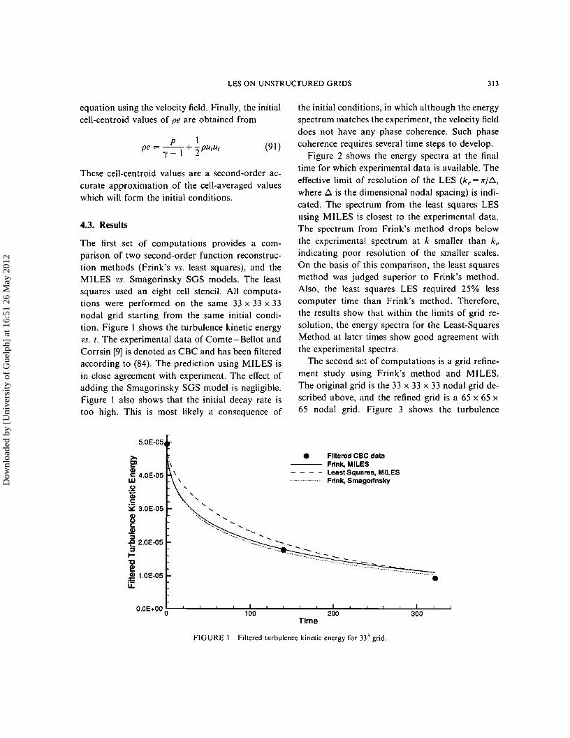
The first set of computations provides a com­parison of two second-order function reconstruc­tion methods (Frink's vs. least squares), and theMILES vs. Smagorinsky SGS models. The leastsquares used an eight cell stencil. All computa­tions were performed on the same 33 x 33 x 33nodal grid starting from the same initial condi­tion. Figure I shows the turbulence kinetic energyvs. I. The experimental data of Comte - Bellot andCorrsin [9] is denoted as CBC and has been filteredaccording to (84). The prediction using MILES isin close agreement with experiment. The effect ofadding the Smagorinsky SGS model is negligible.Figure I also shows that the initial decay rate istoo high. This is most likely a consequence of

the initial conditions, in which although the energyspectrum matches the experiment, the velocity fielddoes not have any phase coherence. Such phasecoherence requires several time steps to develop.

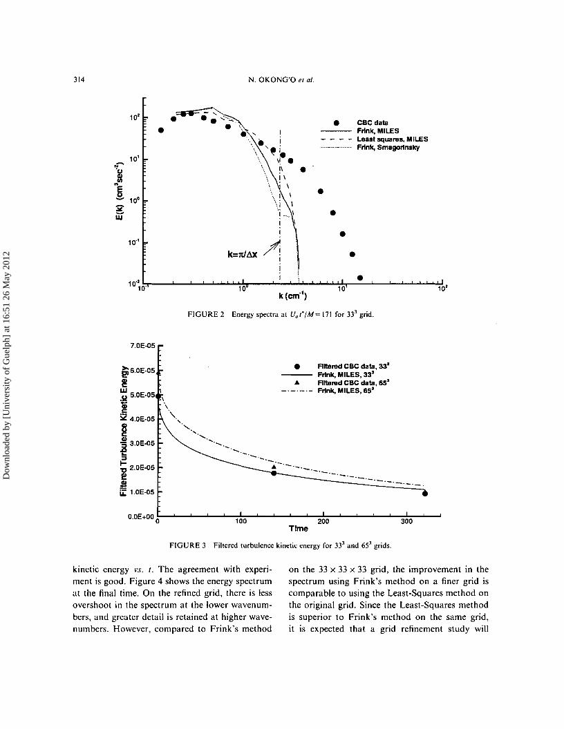
Figure 2 shows the energy spectra at the finaltime for which experimental data is available. Theeffective limit of resolution of the LES (k e =rr/iJ.,where iJ. is the dimensional nodal spacing) is indi­cated. The spectrum from the least squares LESusing MILES is closest to the experimental data.The spectrum from Frink's method drops belowthe experimental spectrum at k smaller than k;indicating poor resolution of the smaller scales.On the basis of this comparison, the least squaresmethod was judged superior to Frink's method.Also, the least squares LES required 25% lesscomputer time than Frink's method. Therefore,the results show that within the limits of grid re­solution, the energy spectra for the Least-SquaresMethod at later times show good agreement withthe experimental spectra.

The second set of computations is a grid refine­ment study using Frink's method and MILES.The original grid is the 33 x 33 x 33 nodal grid de­scribed above, and the refined grid is a 65 x 65 x65 nodal grid. Figure 3 shows the turbulence

(91 )p I

pe = I _ I + 2PUjUj

>. • Filtered CSC datae' Frtnk, MILES

~ 4.0E-05 - - - - Least Squares, MILES

.S!Frtnk, Smagortnsky

a;c:S2 3.0E-05 -,

8 ... -,c:~::l-e 2.0E-05::lI-'tl2!i! 1.0E-05

.........................

i:i: •O.OE+OO 0 I

100 200 300Time

FIGURE J Filtered turbulence kinetic energy for 33' grid.

Dow

nloa

ded

by [

Uni

vers

ity o

f G

uelp

h] a

t 16:

51 2

6 M

ay 2

012

314 N. OKONG'O et al.

•

• CsC dataFrink, MILES

- - - - Least squarus, MILESFrink, Smagorinsky

••

•

I

". I--- '. i\. ":.\ \1.

1\ •I \. \

\

\

.... \\

•10'

;;-

~~! 10':2"W-

10"

10k (em")

•10 10'

FIGURE 2 Energy spectra at Uol'jM= 171 for 333 grid.

-._--

• Rltarud CSC data, 33'--- Frink, MILES, 33'

Flltarud CSC data, 65'Frlnk, MILES, 65'

...... ,._.,....-._._._.-"-.-"-.-"-.-.-.-.

,'-.

7.0E-05

~6.0E-05

l1!w.Y 5.0E-05

!52 4.0E-OS

~GI'S 3.0E-OSof::s...'02.0E-OSI!!

~ 1.0E-05

300200100O.OE+OO 0~""""_...J..._.l-""""-::-!:-:~.l-""""_...J..._.l-~".......J..._.l-""""_...J.......".l:-:-""""-"'"

Time

FIGURE 3 Filtered turbulence kinetic energy for 333 and 653 grids.

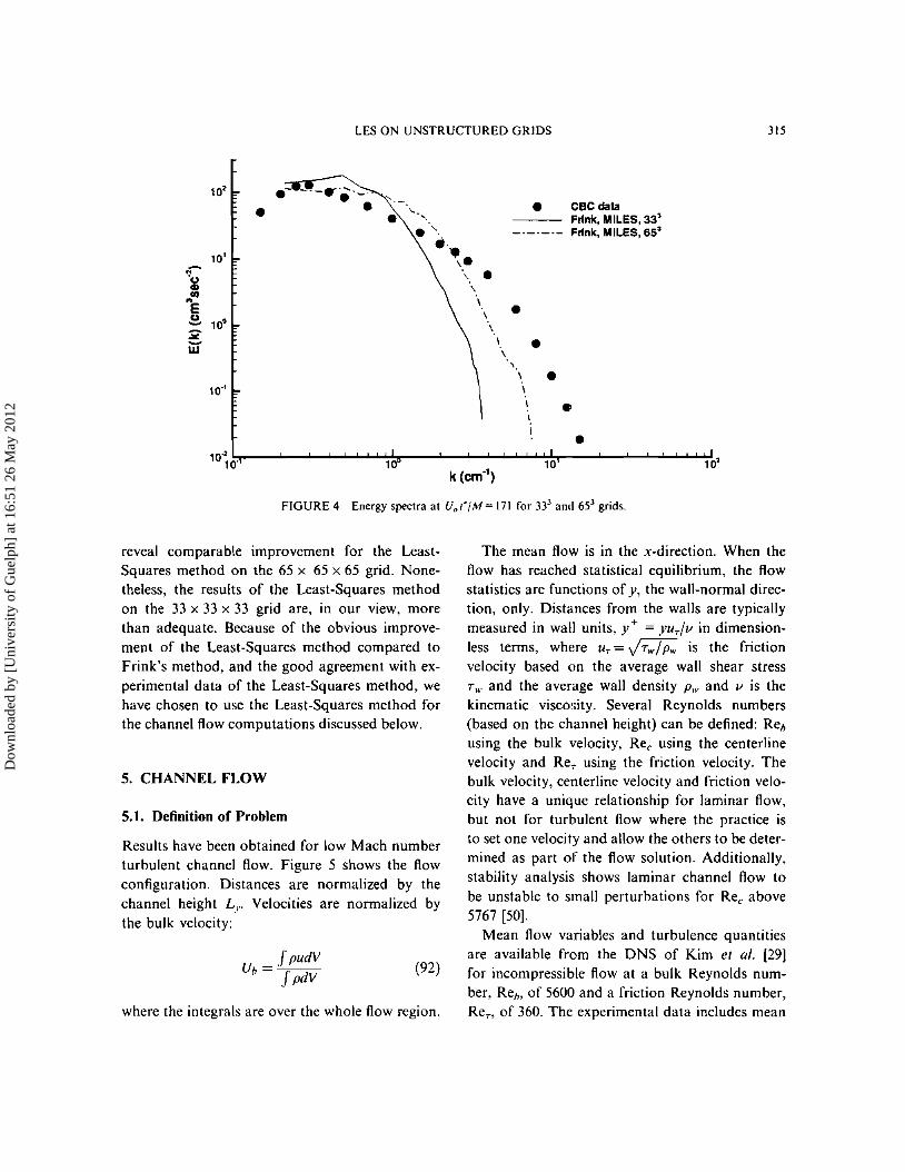
kinetic energy vs. 1. The agreement with experi­ment is good. Figure 4 shows the energy spectrumat the final time. On the refined grid, there is lessovershoot in the spectrum at the lower wavenum­bers, and greater detail is retained at higher wave­numbers. However, compared to Frink's method

on the 33 x 33 x 33 grid, the improvement in thespectrum using Frink's method on a finer grid iscomparable to using the Least-Squares method onthe original grid. Since the Least-Squares methodis superior to Frink's method on the same grid,it is expected that a grid refinement study will

Dow

nloa

ded

by [

Uni

vers

ity o

f G

uelp

h] a

t 16:

51 2

6 M

ay 2

012

LES ON UNSTRUCTURED GRIDS 315

• • esc dataFrink, MILES, 33'.". _._._.- Frink, MILES, 65'•10' ~.

N\ •.~

\etI.. \E •~

\

:>< \

W \ •\ ,\ •10" \

\ •,I •

10;0' 10 10 10'k (em")

FIGURE 4 Energy spectra at U; t"/M = 171 for 333 and 653 grids.

5.1. Definition of Problem

5. CHANNEL FLOW

where the integrals are over the whole flow region.

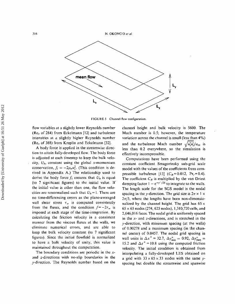
Results have been obtained for low Mach numberturbulent channel flow. Figure 5 shows the flowconfiguration. Distances are normalized by thechannel height L,.. Velocities are normalized bythe bulk velocity:

The mean flow is in the x-direction. When theflow has reached statistical equilibrium, the flowstatistics are functions of y, the wall-normal direc­tion, only. Distances from the walls are typicallymeasured in wall units, y + = yu.]» in dimension­less terms, where Ur=JTw/Pw is the frictionvelocity based on the average wall shear stressT ... and the average wall density P... and v is thekinematic viscosity. Several Reynolds numbers(based on the channel height) can be defined: Re;using the bulk velocity, Re, using the centerlinevelocity and Re7 using the friction velocity. Thebulk velocity, centerline velocity and friction velo­city have a unique relationship for laminar flow,but not for turbulent flow where the practice isto set one velocity and allow the others to be deter­mined as part of the flow solution. Additionally,stability analysis shows laminar channel flow tobe unstable to small perturbations for Re, above5767 [50].

Mean flow variables and turbulence quantitiesare available from the DNS of Kim et al. [29Jfor incompressible flow at a bulk Reynolds num­ber, Re., of 5600 and a friction Reynolds number,ReT> of 360. The experimental data includes mean

(92)JpudV

u, = JpdV

reveal comparable improvement for the Least­Squares method on the 65 x 65 x 65 grid. None­theless, the results of the Least-Squares methodon the 33 x 33 x 33 grid are, in our view, morethan adequate. Because of the obvious improve­ment of the Least-Squares method compared toFrink's method, and the good agreement with ex­perimental data of the Least-Squares method, wehave chosen to use the Least-Squares method forthe channel flow computations discussed below.

Dow

nloa

ded

by [

Uni

vers

ity o

f G

uelp

h] a

t 16:

51 2

6 M

ay 2

012

316 N. OKONG'O et al.

FIGURE 5 Channel flow configuration.

flow variables at a slightly lower Reynolds number(ReT of 284) from Eckelmann [12] and turbulenceintensities at a slightly higher Reynolds number(ReT of 388) from Kreplin and Eckelmann [32].

A body force is applied in the streamwise direc­tion to attain fully-developed flow. The body forceis adjusted at each timestep to keep the bulk velo­city, Ui, constant using the global x-momentumconservation, II = -2p",u;. (This condition is de­rived in Appendix A.) The relationship used toderive the body force II ensures that Uh is equal(to 7 significant figures) to the initial value. Ifthe initial value is other than one, the flow velo­cities are renormalized such that U; = I. There areno time-differencing errors as the plane-averagedwall shear stress r., is computed consistentlyfrom the fluxes, and the condition 1= -2r", isimposed at each stage of the time-integration. Bycalculating the friction velocity in a consistentmanner from the viscous fluxes at the walls, weeliminate numerical errors, and are able tokeep the bulk velocity constant (to 7 significantfigures). Since the initial flowfield is normalizedto have a bulk velocity of unity, this value ismaintained throughout the computation.

The boundary conditions are periodic in the x­and z-directions with no-slip boundaries in thej-dircction. The Reynolds number based on the

channel height and bulk velocity is 5600. TheMach number is 0.5; however, the temperaturevariation across the channel is small (less than 4%)

and the turbulence Mach number ~/aoo isless than 0.2 everywhere, so the simulation iseffectively incompressible.

Computations have been performed using theconstant coefficient Smagorinsky sub-grid scalemodel with the values of the coefficients from com­pressible turbulence [13] (C R=0.012, Pr,=OA).The coefficient CR is multiplied by the van Driestdamping factor I - e-Y+ /26 to integrate to the walls.The length scale for the SGS model is the nodalspacing in the j-direction. The grid size is 211' x I x211'/3, where the lengths have been non-dimensio­nalized by the channel height. The grid has 65 x65 x 65 nodes (274, 625 nodes), 1,310,720 cells, and2,646,016 faces. The nodal grid is uniformly spacedin the x- and z-directions, and is stretched in thej-direction, with minimum spacing (at the walls)of 0.00278 and a maximum spacing (in the chan­nel center) of 0.0457. The nodal grid spacing inwall units is box+ = 32.7, boY~in = 0.92, boY~ax =15.2 and boz+ = 10.8 using the computed frictionvelocity. The initial condition is obtained frominterpolating a fully-developed LES obtained ona grid with 33 x 65 x 33 nodes with the same y­

spacing but double the streamwise and spanwise

Dow

nloa

ded

by [

Uni

vers

ity o

f G

uelp

h] a

t 16:

51 2

6 M

ay 2

012

LES ON UNSTRUCTURED GRIDS 317

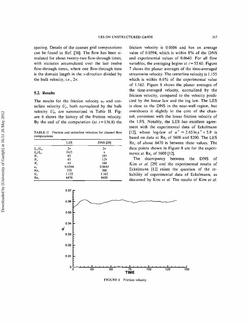
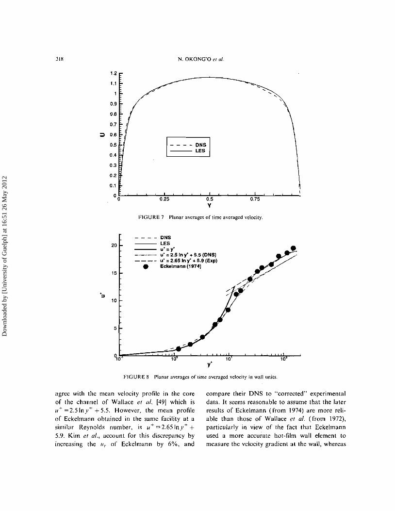
friction velocity is 0.0606 and has an averagevalue of 0.0594, which is within 8% of the DNSand experimental values of 0.0643. For all flowvariables, the averaging begins at 1=55.60. Figure7 shows the planar averages of the time-averagedstreamwise velocity. The centerline velocity is 1.155which is within 0.6% of the experimental valueof 1.162. Figure 8 shows the planar averages ofthe time-averaged velocity, normalized by thefriction velocity, compared to the velocity predi­cted by the linear law and the log law. The LESis close to the DNS in the near-wall region, butovershoots it slightly in the core of the chan­nel, consistent with the lower friction velocity ofthe LES. Notably, the LES has excellent agree­ment with the experimental data of Eckelmann[12], whose log-law of 11+ = 2.65Iny+ +5.9 isbased on data at Re, of 5600 and 8200. The LESRe, of about 6470 is between these values. Thedata points shown in Figure 8 are for the experi­ments at Rec of 5600 [12].

The discrepancy between the DNS ofKim et al. [29] and the experimental results ofEckelmann [12] raises the question of the re­liability of experimental data of Eckelmann, asdiscussed by Kim et al. The results of Kim et al.

The results for the friction velocity liT and cen­terline velocity Ve , both normalized by the bulkvelocity Ui; are summarized in Table II. Fig­ure 6 shows the history of the friction velocity.By the end of the computation (at t = 136.8) the

LES DNS [291

L"fLy h hL,fL,. 21ff3 1f

NT 65 192N,. 65 129N, 65 160UT 0.0594 0.0643ReT 330 360U, 1.155 1.162Re, 6470 6600

0.07

0.06

0.05

0.04

::r0.03

0.02

0.Q1

00

TABLE II Friction and centerline velocities for channel flowcomputations

spacing. Details of the coarser grid computationscan be found in Ref. [38]. The flow has been si­mulated for about twenty-two flow-through times,with statistics accumulated over the last twelveflow-through times, where one flow-through timeis the domain length in the x-direction divided bythe bulk velocity, i.e., 2Jr.

5.2. Results

FIGURE 6 Friction velocity.

Dow

nloa

ded

by [

Uni

vers

ity o

f G

uelp

h] a

t 16:

51 2

6 M

ay 2

012

318 N. OKONG'O et al.

1.1

0.9

0.8

0.7

::::l 0.6

0.5

0.4

0.3

0.2

0.1

00 0.25 0.5Y

0.75

FIGURE 7 Planar averages of time averaged velocity.

1010

ONSLESu' =y'u" =2.5 In v: + 5.5 (ONS)u· =2.65 In y' + 5.9 (Exp)Eckelmann (1974)•

.:>

FIGURE M Planar averages of time averaged velocity in wall units.

agree with the mean velocity profile in the coreor the channel or Wallace et al. [49] which isIt+ =2.5Iny+ +5.5. However, the mean profileor Eckelmann obtained in the same facility at asimilar Reynolds number, is It + = 2.651n y + +5.9. Kim et al., account for this discrepancy byincreasing the u, or Eckelmann by 6%, and

compare their DNS to "corrected" experimentaldata. It seems reasonable to assume that the laterresults or Eckelmann (from 1974) are more reli­able than those or Wallace et al. (from 1972),particularly in view or the fact that Eckelmannused a more accurate hot-film wall element tomeasure the velocity gradient at the wall, whereas

Dow

nloa

ded

by [

Uni

vers

ity o

f G

uelp

h] a

t 16:

51 2

6 M

ay 2

012

LES ON UNSTRUcrURED GRIDS 319

Wallace et al., used a hot-film probe. Hence, weconsider the experimental data of Eckelmannreliable enough, and note that the above-men­tioned discrepancy of 6% in the friction velocityis well within the error range typically acceptedin engineering problems.

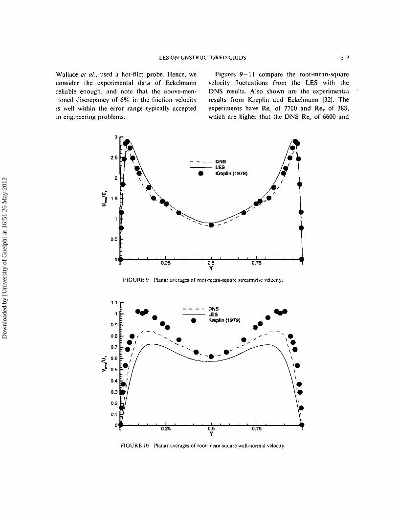
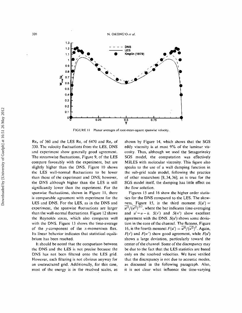
Figures 9-11 compare the root-mean-squarevelocity fluctuations from the LES with theDNS results. Also shown are the experimentalresults from Kreplin and Eckelmann [32]. Theexperiments have Re" of 7700 and ReT of 388,which are higher that the DNS Re, of 6600 and

•

3

2.5

2

0.5

DNS--- LES

Kreplln (1979)

FIGURE 9 Planar averages of root-mean-square streamwise velocity.

1.1

¥.- - -- DNS

.¥LES

• Kreplln (1979)0.9 •• ••0.8 '-

-,.I.

0.7 I.I

=>" 0.6 I

) 0.5I.II

0.4I.

0.3 I.I

0.2 I•0.1 I

00.25 0.5 0.75

Y

FIGURE 10 Planar averages of root-mean-square wall-normal velocity.

Dow

nloa

ded

by [

Uni

vers

ity o

f G

uelp

h] a

t 16:

51 2

6 M

ay 2

012

N. OKONG'O et al.

0.75

- - - - DNSLES

• Kreplln (1979)

025 O~

Y

320

1.3

1.2

1.1

0.9

0.8

:>" 0.7

) 0.6

0.5

0.4

0.3

0.2

0.1

0

FIGURE II Planar averages of root-mean-square spanwise velocity.

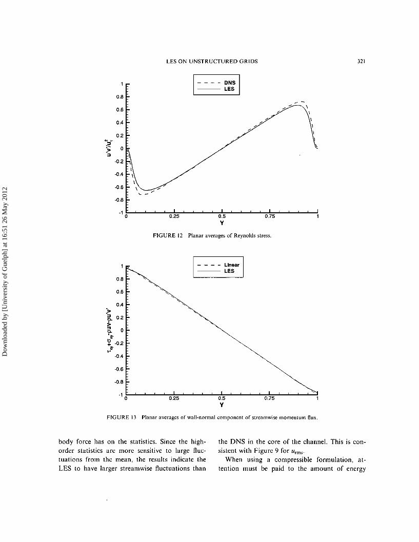
ReT of 360 and the LES Re, of 6470 and ReT of330. The velocity fluctuations from the LES, DNSand experiment show generally good agreement.The streamwise fluctuations, Figure 9, of the LEScompare favorably with the experiment, but areslightly higher than the DNS. Figure 10 showsthe LES wall-normal fluctuations to be lowerthan those of the experiment and DNS; however,the DNS although higher than the LES is stillsignificantly lower than the experiment. For thespanwise fluctuations, shown in Figure II, thereis comparable agreement with experiment for theLES and DNS. For the LES, as in the DNS andexperiment, the spanwise fluctuations are largerthan the wall-normal fluctuations. Figure 12 showsthe Reynolds stress, which also compares wellwith the DNS. Figure 13 shows the time-averageof the y-component of the x-momentum flux.Its linear behavior indicates that statistical. equili­brium has been reached.

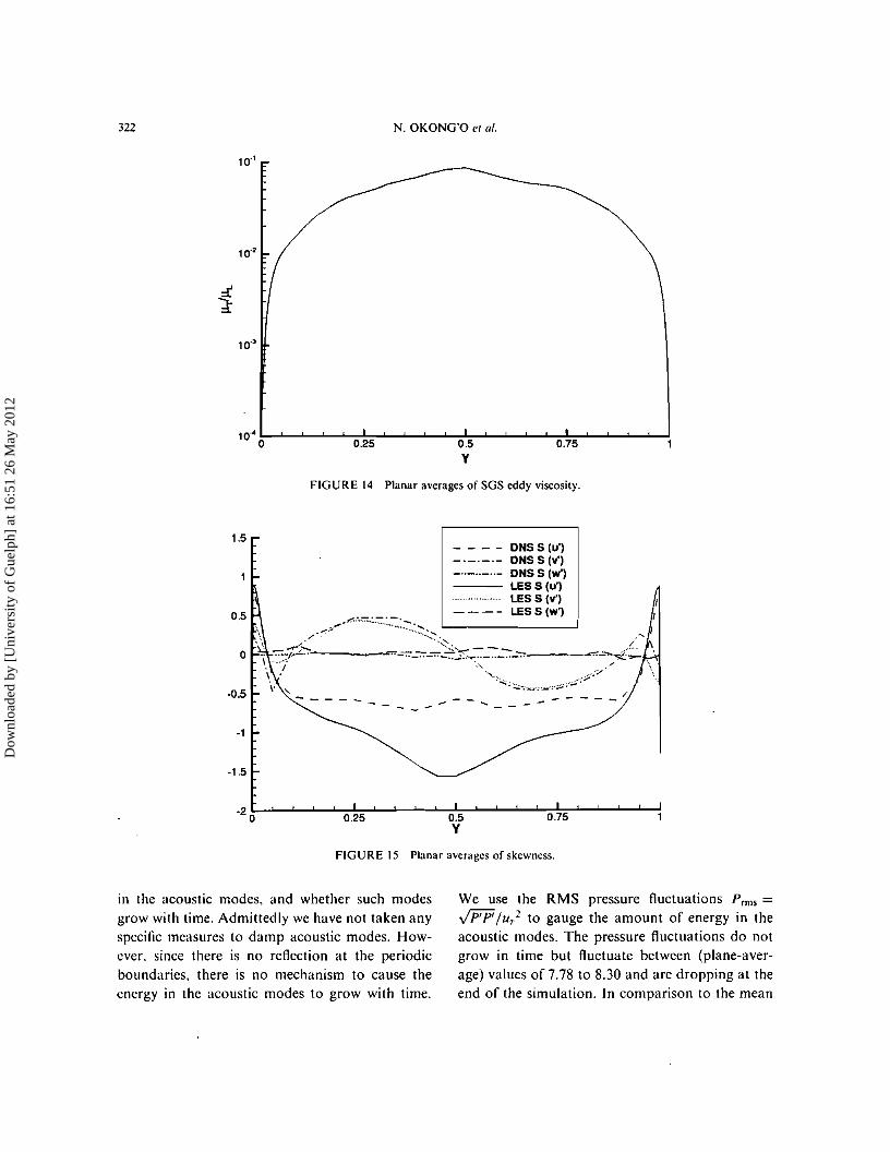
It should be noted that the comparison betweenthe DNS and the LES is not precise because theDNS has not been filtered onto the LES grid.However, such filtering is not obvious anyway foran unstructured grid. Additionally, for this case,most of the energy is in the resolved scales, as

shown by Figure 14, which shows that the SGSeddy viscosity is at most 9% of the laminar vis­cosity. Thus, although we used the SmagorinskySGS model, the computation was effectivelyMILES with molecular viscosity. This figure alsospeaks to the use of a wall damping function inthe sub-grid scale model, following the practiceof other researchers [8,34,36]; as is true for theSGS model itself, the damping has little effect onthe flow solution.

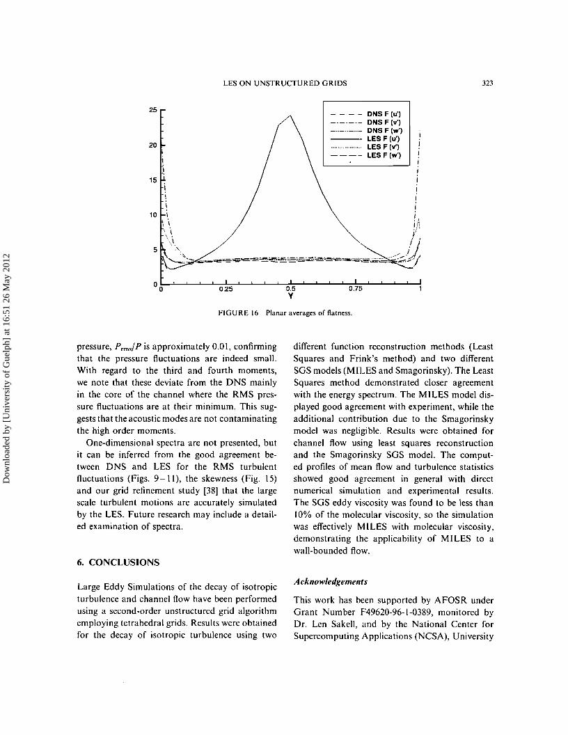
Figures 15 and 16 show the higher order statis­tics for the DNS compared to the LES. The skew­ness, Figure 15, is the third moment S(u') =u,3/(u,2)3/2, where the bar indicates time-averagingand u' = u - ii. S(v') and S(lIt ) show excellentagreement with the DNS. S(u') shows some devia­tion in the core of the channel. The flatness, Figure16, is the fourth moment F(u') = U,4/(u'2f Again,F(v') and F(w') show good agreement, while F(u')shows a large deviation, particularly toward thecenter of the channel. Some of the discrepancy maybe due to the fact that the LES statistics are basedonly on the resolved velocities. We have verifiedthat the discrepancy is not due to acoustic modes,as discussed in the following paragraph. Also,it is not clear what influence the time-varying

Dow

nloa

ded

by [

Uni

vers

ity o

f G

uelp

h] a

t 16:

51 2

6 M

ay 2

012

LES ON UNSTRUCTURED GRIDS 321

0.8

0.6

0.4

0.2N "~:; 0~

-0.2

-0.4

-0.6

-0.8

-1 0

FIGURE 12 Planar averages of Reynolds stress.

LinearLES1----

-0.6

0.4

0.8

-1 0 0.25

0.6

-0.8

:.>E. 0.2:I-~ 0~r;+ -0.2r;.' -0.4

FIGURE 13 Planar averages of wall-normal component of streamwise momentum flux.

body force has on the stausucs, Since the high­order statistics are more sensitive to large fluc­tuations from the mean, the results indicate theLES to have larger streamwise fluctuations than

the DNS in the core of the channel. This is con­sistent with Figure 9 for Urms '

When using a compressible formulation, at­tention must be paid to the amount of energy

Dow

nloa

ded

by [

Uni

vers

ity o

f G

uelp

h] a

t 16:

51 2

6 M

ay 2

012

322

10"

N. OKONG'O et al.

FIGURE 14 Planar averages of SGS eddy viscosity.

1.5

0.5

o

-0.5

-1

-1.5

DNSS (u')DNS S (v')DNSS (w')LES S (u')LES S (v')LES S (w')

FIGURE 15 Planar averages of skewness.

in the acoustic modes, and whether such modesgrow with time. Admittedly we have not taken anyspecific measures to damp acoustic modes. How­ever. since there is no reflection at the periodicboundaries, there is no mechanism to cause theenergy in the acoustic modes to grow with time.

We use the RMS pressure fluctuations Prms =JplPI lUTz to gauge the amount of energy in theacoustic modes. The pressure fluctuations do notgrow in time but fluctuate between (plane-aver­age) values of 7.78 to 8.30 and are dropping at theend of the simulation. In comparison to the mean

Dow

nloa

ded

by [

Uni

vers

ity o

f G

uelp

h] a

t 16:

51 2

6 M

ay 2

012

- - - .- DNS F (u')_._._.- DNS F (v')_ .._ .._ ..- DNS F (w')---- LESF(u')

LES F (v')---- LES F (w')

25

20

15

10

5

LES ON UNSTRUCTURED GRIDS

IJ

J

IIIIII

IiA(

..__..="",.=..,""~~'§'§s.="",.",,=,,,,,"s;;;r~~

323

FIGURE 16 Planar averages of flatness.

pressure, Prms/P is approximately 0.01, confirmingthat the pressure fluctuations are indeed small.With regard to the third and fourth moments,we note that these deviate from the DNS mainlyin the core of the channel where the RMS pres­sure fluctuations are at their minimum. This sug­gests that the acoustic modes are not contaminatingthe high order moments.

One-dimensional spectra are not presented, butit can be inferred from the good agreement be­tween DNS and LES for the RMS turbulentfluctuations (Figs. 9-11), the skewness (Fig. 15)and our grid refinement study [38] that the largescale turbulent motions are accurately simulatedby the LES. Future research may include a detail­ed examination of spectra.

6. CONCLUSIONS

Large Eddy Simulations of the decay of isotropicturbulence and channel flow have been performedusing a second-order unstructured grid algorithmemploying tetrahedral grids. Results were obtainedfor the decay of isotropic turbulence using two

different function reconstruction methods (LeastSquares and Frink's method) and two differentSGS models (MILES and Smagorinsky). The LeastSquares method demonstrated closer agreementwith the energy spectrum. The MILES model dis­played good agreement with experiment, while theadditional contribution due to the Smagorinskymodel was negligible. Results were obtained forchannel flow using least squares reconstructionand the Smagorinsky SGS model. The comput­ed profiles of mean flow and turbulence statisticsshowed good agreement in general with directnumerical simulation and experimental results.The SGS eddy viscosity was found to be less than10% of the molecular viscosity, so the simulationwas effectively MILES with molecular viscosity,demonstrating the applicability of MILES to awall-bounded flow.

Acknowledgements

This work has been supported by AFOSR underGrant Number 1"49620-96-1-0389, monitored byDr. Len Sakell, and by the National Center forSupercomputing Applications (NCSA), University

Dow

nloa

ded

by [

Uni

vers

ity o

f G

uelp

h] a

t 16:

51 2

6 M

ay 2

012

324 N. OKONG'O ct al.

of Illinois at Urbana-Champaign, under GrantNumbers ENG98000lN and CTS980021N.Computations were performed on the NCSA CrayOrigin2000, the NA VO OCEANO DOD CrayOrigin2000 and an SGI Power Onyx at RutgersUniversity. The results were analyzed at the RutgersUniversity Supercomputer Remote Access Center.We would like to thank Robert Murray and VijayShukla for their assistance with the flow visualiza­tions. We would also like to thank Jay Boris, GaryColeman, Dan Haworth, Ken Jansen, ThomasLund and Elaine Oran for their suggestions andcomments.

Reference..,

III Abramowitz, M. and Stegun, I. A., Editors. Handbook ofMathematical Functions with Formulas, Graphs and Math­ematical Tables, John Wiley & Sons, New York, 1972.pp.893-5.

[21 Akselvoll, K. and Moin, P. (1996). Large Eddy Simulationof Turbulent Conlined Coannular Jets. Journal of FluidMechanics, 315, 387-411.

[3] Bnlnms. E., Bcnocci, C. and Piomelli, U. (1996). Two­Layer Approximate Boundary Conditions for Large EddySimulation. AIAA Journal, 34. 1111-1119.

[4] IIjorek, A. (1996). Numerical Methods for Least SquaresProblems, pages 9. 10. 15. Society for Industrial and Ap­plied Mathematics (SIAM).

[5] Boris, J. P., Grinstein, F. F., Oran, E. S. and Kolbe, R. L.(1992). New Insights into Large Eddy Simulation. FluidOvnumics Research, 10, 199-228.

16) lIurden. R. L. and Faires. J. D. (1989). Numerical Analy­sis. PWS·KENT, Boston. 4th edition.

(7) Canute, c., Hussaini, M. Y., Quarteroni, A. and Zang,T. A., Spectral Methods in Fluid Dynamics. Springer­Verlag, New York, 1988.

(8) Ciofalo, M. and Collins, M. (1992). Large Eddy Simula­tion of Turbulent Flow and Heat Transfer in Plane andRib-Roughened Channels. International Journal for Nu­merical Methods ill fluids. 15.453-489.

[91 Comtc-Bcllot, G. and Corrsin, S. (1971). Simple EulerianTime Correlation of Full- and Narrow-Band VelocitySignals in Grid-Generated "Isotropic" Turbulence.Journal of Fluitt Mechanics, 48(2), 273- 337.

[10] Deardorff. J. W. (1970). A Numerical Study of Three­Dimensional Turbulent Channel Flow at Large ReynoldsNumbers. Journal of Fluid Mechanics, 41, 453-480.

[II] Denaro. F. M. (1996). Towards a New Model-FreeSimulation of High-Reynolds-Flows: Local AverageDirect Numerical Simulation. International Journal forNumerical Methods ill Fluids. 23, 125-142.

(12] Eckclmann, H. (1974). The Structure of the ViscousSublaycr and the Adjacent Wall Region in a TurbulentChannel Flow. Journal of Fluid Mechanics, 65, 439 -459.

[13] Erlcbachcr, G .• Hussaini, M. Y.. Speziale, C. G. andZang. T. A. (1992). Toward the Large Eddy Simulationof Compressible Turbulent Flows. Journal of FluidMahallic,\",238.155-185.

(14) Ferziger, J. (1997). Large Eddy Simulation: An Introduc­tion and Perspective. In: Metais, O. and Ferziger, J.,Editors, Nell' Tools in Turbulence Modelling, Chapter 2,pp. 29-47. Springer-Verlag.

(15] Frink, N. T. (1992). Upwind Scheme for Solving the EulerEquations on Unstructured Tetrahedral Meshes. AIAAJournal, 30(1), 70-77.

[16] Frink, N. T. (1994). Recent Progress Toward a Three­Dimensional Unstructured Navier-Stokes Flow Solver.AIAA 94-0061.

(17] Fureby, C. (1996). On Subgrid Scale Modelling in LargeEddy Simulations of Compressible Fluid Flow. Physics ofFluids, 8(5), 1301-1311.

(l8J Fureby, C. and Moller, S.-1. (1995). Large Eddy Simula­tion of Reacting Flows Applied to Bluff Body StabilizedFlames. AIAA Journal, 33(12), 2339-2347.

(19) Galperin, B. and Orszag, S. A., Editors. (1993). LargeEddy Simulation of Complex Engineering and GeophysicalFlows. Cambridge University Press.

[20] Germano, M.. Plomelli, U., Moin, P. and Cabot, W.(199\). A Dynamic Subgrid-scale Eddy Viscosity Model.Physics of Fluids, A, 3, 1760-1765.

[21] Golub, G. and Van Loan. C. (1989). Matrix Computa­tions. Johns Hopkins University Press, Baltimore. MD.2nd edition.

[22] Gottlieb, J. J. and Groth, C. P. T. (1988). Assessment ofRiemann Solvers for Unsteady One-Dimensional InviscidFlows of Perfect Gases. Journal of Computational Physics.78.437-458.

(23) Grinstein, F. and DeVore, C. (1996). Dynamics of Co her­ent Structures and Transition to Turbulence in FreeSquare Jets. Physics of Fluids, 8(5), 1237-1251.

(24) Gropp, W., Lusk, E. and Skjellum, A. (\ 994). Using M PI:Portable Parallel Programming with the Message-PassingInterface. MIT Press, Cambridge, MA.

[25] Haworth, D. C. and Jansen, K.. Large Eddy Simulationon Unstructured Deforming Meshes: Towards Recipro­cating IC Engines. Center for Turbulence Research, Sum­mer Program. 1996. Submitted to Computers and Fluids.

[26] Hirsch, C. (1988). Numerical Computation of Internal andExternal Flows, Volume 2: Computational Methods forInviscid and Viscous Flows. Wiley.

[27] Jansen, K., Large Eddy Simulation Using Unstruc­tured Grids. In: Liu, C.; Liu, Z. and Sakell, L., Editors,Advances in DNSjLES, pages 117-128. Greyden Press,Columbus, Ohio, 1997, Proceedings of the First AFOSRInternational Conference on DNS/LES. Louisiana TechUniversity, Ruston, Louisiana, August, 1997. pp. 4-8.

(28) Kergaravat, Y., Jacon, F., Okong'o, N. and Knight. D.(1998). A Fully-Implicit 2-D Navier-Stokes Algorithmfor Unstructured Grids. International Journal for Compu­tational fluid Dynamics, 9, 179- 196.

[29J Kim, J., Moin, P. and Moser, R. (1987). Turbulence Sta­tistics in Fully Developed Channel Flow at Low Rey­nolds Number. Journal of Fluid Mechanics, 177, 133-166.

(30) Knight, D. D. (\994). A Fully Implicit Navier-StokesAlgorithm Using an Unstructured Grid and FluxDifference Splitting. Applied Numerical Mathematics,16,101-128.

[31) Knight, D. D., Zhou, G., Okong'o, N. and Shukla, V.(1998). Compressible Large Eddy Simulation UsingUnstructured Grids. AIAA 98-0535.

132] Kreplin, H. and Eckclmann, H. (1979). Behavior of theThree Fluctuating Velocity Components in the WallRegion of a Turbulent Channel Flow. Physics of Fluids,22(7), 1233- 1239.

Dow

nloa

ded

by [

Uni

vers

ity o

f G

uelp

h] a

t 16:

51 2

6 M

ay 2

012

LES ON UNSTRUCTURED GRIDS 325

This implies that the bulk density Ph

APPENDIX A: BODY FORCEFOR CHANNEL FLOW

dd rpdV + r pu· iidA = 0 (93)flv lliV

(96)

(95)

dd rpdV + r PWlxdA +1 pvn)'dA

f lv J'=O,L ),=0,1

+ l=o,w pwn=dA = O' (94)

Here u is the (filtered, Favre-averaged) velocityand ii is the area outward normal. Applyingthe no-slip boundary conditions on the lop (y = 0)and bottom (y= I) surfaces, and periodic bound­ary conditions on the remaining four surfaces (theupstream x = 0 surface is periodic to the down­stream x = LxiL; = L surface, and the spanwisez = 0 surface is periodic to the z = L=IL; = Wsurface):

The body force is adjusted at each time-step tokeep the bulk velocity constanl. The flow config­uration is shown in Figure 5; the lengths arenon-dimensionalized by L, .. Beginning with thedimensionless global integral constraints, Eq. (23)over the entire flow domain, the conservation ofmass is:

The third term is zero and the contributions fromthe periodic faces cancel each other (the velocitiesare the same, but the normal vectors point in op­posite directions), leaving only the first term:

is constant. Using the bulk density as the referencedensity Poe means that the bulk density will be one.

Since the body force is only in the x-direction,only the conservation of x-momentum from

[33] Martinelli. L. and Jameson. A. (1988). Validation of aMuitigrid Method for the Reynolds Averaged Equations.A/AA 88-0414.

[34J Mason, P. J. and Callen, N. S. (1986). On the Magni­tude of the Subgrid-Scale Eddy Coefficient in Large EddySimulations of Turbulent Channel Flow. Journal of FluidMechanics, 162,439-462.

[351 Meneveau, c., Lund, T. and Cabot, W. (1996). ALagrangian Dynamic Subgrid-Scale Model of Turbu­lence. Journal of Fluid Mechanics, 319. 353-385.

[361 Moin, P. and Kim, J. (1982). Numerical Investigation ofTurbulent Channel Flow. Journal of Fluid Mechanics, 118,341-377.

[37] Moin, P., Squires, K.. Cabot, W. and Lee, S. (1991).A Dynamic Subgrid-Scale Model for CompressibleTurbulence and Scalar Transport. Physics of Fluidv, 3.2746-2757.

[38] Okongo, N., Time-Accurate Unstructured Grid Algo­rithms for the Compressible Navier Stokes Equations.Ph.D. Thesis. Mechanical and Aerospace Engineering,Rutgers, The State University of New Jersey, October,1998.

[39) Okong'o, N. and Knight, D. D. (1998). Implicit Un­structured Navicr-Stokes Simulation of Leading EdgeSeparation oyer a Pitching Airfoil. Applied NumericalMathematics. 27(3), 268-308.

[40] Ollivier-Gooch, C. F. (1997). High-Order ENO Schemesfor Unstructured Meshes Based on Least Squares Recon­struction. A/AA 97-0540.

[411 Oran, E. and Boris, J., Computing Turbulent ShearFlows - A Convenient Conspiracy. Computers in Physics.7(5), 523 - 533, September/October, 1993.

[42] Porter, D.• Bouquet, A. and Woodward, P. (1994).Kolrnogorov-like Spectra in Decaying Three-Di­mensional Supersonic Flows. Physics of Fluids. 6(6),2133-2142.

[43] Rausch, R., Batina. J. and Yang, H. (1991). SpatialAdaption Procedures on Unstructured Meshes forAccurate Unsteady Aerodynamic Flow Computation.AIAA 91-1/06.

[44) Simons, T. and Pletcher, R. (I 998). Large Eddy Simula­tion of Turbulent Flows Using Unstructured Grids. A/AA98-3314.

[45] Smagorinsky, J. (1993). Some Historical Remarks on theUse of Nonlinear Viscosities. In: Galperin, B. and Orszag,S. A. Editors, Large Eddy Simulation of Complex Engi­neering and Geophysical Flows, Chapter 1, pp. 3 - 36.Cambridge University Press.

[461 Spyropoulos, E. and Blaisdell, G. (1995). Evaluationof the Dynamic Subgrid-Scale Model for Large EddySimulations of Compressible Turbulent Flows. A/AA95-0355.

[47] Toro, E.. Riemann Solvers and Numerical Methods forFluid Dynamics. Springer-Verlag, Berlin, 1997.

[48] Venkatakrishnan, V. (1996). Perspective on UnstructuredGrid Flow Solvers. AIAA Journal, 34(3), 533-547.

[49J Wallace, 1. M., Eckelmann, H. and Brodkey, R. S. (1972).The Wall Region in Turbulent Shear Flow. Journal ofFluid Mechanics, 54(1),39-48.

[50J White, F. M. (1991). Viscous Fluid ns«. Me-Graw-Hill.[51] Wu, X. and Squires, K. (1997). Large Eddy Simulation of

an Equilibrium Three-Dimensional Turbulent BoundaryLayer. A/AA Journal. 35, 67-74.

[52] Yang, K.-S. and Ferziger, J. (1993). Large Eddy Simula­tion of Turbulent Obstacle Flow Using a DynamicSubgrid-Scale Model. AIAA Journal. 31, 1406- 1413.

Dow

nloa

ded

by [

Uni

vers

ity o

f G

uelp

h] a

t 16:

51 2

6 M

ay 2

012

326 N. OKONO'O et al.

Applying the no-slip and periodic boundaryconditions as before leaves

Eq. (23) is needed:

d rpudV + r!ldV + r(puii· n+ pnx)dA(II Jv .Iv J.v

=1[T.,·x n.\. + Txyn)' + Txznz]dA (97)w

au, I 1Pb-+!I =- TxynydA = -2T...dt LW y=O,1

( 100)

Defining the bulk velocity Ub as

U Iv pudV I r IV (98)b = IvpdV = Pb V Jv PU

{

where the volume V= LW, and applying a spatial­ly uniform body force II

LW (Pb dUb +/1) +1 (pu2n.\. + p - T.u)dAdt x=O.1-

+ 1=:0.1 (puvn,.)dA + l=o,w ipuwn, - T.\z)dA

= r T,ydA (99)./y=O,1

which includes the definition of the wall shearstress T ... as the average of the shear stress on thetop and bottom surfaces. The friction velocity isrelated to the wall shear stress as UT = }T.../pw­

Then to maintain a constant bulk velocity, dUb/

dt = 0, we require

!I = -2Tw = -2pwu; (101)

When using explicit multi-stage time integration,this condition is applied at each stage during eachtimestep.

Dow

nloa

ded

by [

Uni

vers

ity o

f G

uelp

h] a

t 16:

51 2

6 M

ay 2

012