Conjugate Heat Transfer for the Unsteady Compressible

Navier-Stokes Equations Using a Multi-block Coupling

Jan Nordstrom†∗

Department of Mathematics, Linkoping University, SE-581 83 Linkoping, Sweden

Jens Berg†

Department of Information Technology, Uppsala University, SE-751 05, Uppsala, Sweden

Abstract

This paper deals with conjugate heat transfer problems for the time-dependent com-pressible Navier-Stokes equations. One way to model conjugate heat transfer is tocouple the Navier-Stokes equations in the fluid with the heat equation in the solid.This requires two different physics solvers. Another way is to let the Navier-Stokesequations govern the heat transfer in both the solid and in the fluid. This simplifiescalculations since the same physics solver can be used everywhere.

We show by energy estimates that the continuous problem is well-posed whenimposing continuity of temperature and heat fluxes by using a modified L2-equivalentnorm. The equations are discretized using finite difference on summation-by-partsform with boundary- and interface conditions imposed weakly by the simultaneousapproximation term. It is proven that the scheme is energy stable in the modifiednorm for any order of accuracy.

We also show what is required for obtaining the same solution as when the un-steady compressible Navier-Stokes equations are coupled to the heat equation. Thedifferences between the two coupling techniques are discussed theoretically as wellas studied numerically, and it is shown that they are indeed small.

Keywords: Conjugate heat transfer, Navier-Stokes, compressible, unsteady, heatequation, finite difference, summation-by-parts, weak interface conditions, weakmulti-block conditions, stability, high order accuracy

∗Corresponding author: Jan Nordstrom, E-mail: jan.nordstrom@liu.se†Parts of this work were completed while the authors visited the Centre for Turbulence Research

at Stanford University

Preprint submitted to Elsevier November 22, 2012

1. Introduction

Heat transfer is an important factor in many fluid dynamics applications. Flowsare often confined within some material with heat transfer properties. Wheneverthere is a temperature difference between the fluid and the confining solid, heat willbe transferred and change the flow properties in a non-trivial way. This interactionand heat exchange is referred to as the conjugate heat transfer problem [1, 2, 3, 4].Examples of application areas include cooling of turbine blades and nuclear reactors,atmospheric reentry of spacecrafts and gas propulsion micro thrusters for precisesatellite navigation.

Conjugate heat transfer problems have been computed using a variety of methods.For stationary problems, methods include the finite volume method [5], the finiteelement method [6, 7] and the Semi-Implicit Method for Pressure-Linked Equations(SIMPLE) [8]. For unsteady problems, overlapping grids [3] and finite differencemethods [1] have been used. The interface conditions have been imposed eitherstrongly, weakly or by a mixture of both.

There are many ways in which conjugate heat transfer problems can be analyzedand computed. Giles [1] considered the simplified case of two coupled heat equationsand performed a stability analysis which put restrictions on how to chose the interfaceconditions. Henshaw and Chand [3] performed numerical simulations of incompress-ible, temperature dependent fluids with the Boussinesq approximation coupled withthe heat equation. The stability analysis was restricted to the case of two coupledheat equations. Stability and second order accuracy for the coupled model problemwas proven, together with a numerical accuracy study of the full coupled problemshowing second order accuracy, as expected. In [7] a steady, compressible fluid withheat transfer properties is considered and it is stated that accuracy is a key elementin computational heat transfer. The authors develop an adaptive strategy with errorestimators, showing at most second order accuracy.

When reviewing the literature on conjugate heat transfer problems, one can con-clude that for incompressible problems, the heat transfer part is either modeled bythe heat equation, or by using the incompressible Navier-Stokes equations also inthe solid region. The latter strategy is possible since the energy equation in the in-compressible Navier-Stokes equations decouples from the continuity- and momentumequations. In the compressible flow case, the situation is different and more compli-cated. Two major differences exist. Firstly, the energy equation does not decouplefrom the continuity- and momentum equations. Secondly, for compressible fluids,steady problems are mostly considered since the stability of the coupling becomesan issue.

2

The numerical methodology presented in this paper is based on a finite differ-ence on Summation-By-Parts (SBP) form with the Simultaneous ApproximationTerm (SAT) for imposing the boundary and interface conditions weakly. The SBP-SAT method has been used for a variety of problems and has proven to be robust[9, 10, 11, 12, 13, 14, 15]. The SBP finite difference operators were originally con-structed by Kreiss and Schearer [16] with the purpose of constructing an energystable finite difference method [17]. Together with the weak imposition of boundary[18] and interface [19] conditions, the SBP-SAT provides a method for constructingenergy stable schemes for well-posed initial-boundary value problems [20]. Thereare SBP operators based on diagonal norms for the first [21] and second [22, 23]derivative accurate of order 2, 3, 4 and 5, and the stability analysis we will presentis independent of the order of accuracy.

From an implementational point of view, coupling the compressible Navier-Stokesequations to the heat equation is complicated as different solvers are required in thefluid and solid domains. With two different solvers, two different codes, are requiredand data has to be transferred between them by using possibly a third code [24].

A less complicated method would be to only use the Navier-Stokes equationseverywhere and modify an already existing multi-block coupling [12] such that heatis transferred between the fluid and solid domains. In the blocks marked as solids,it is possible to construct initial and boundary conditions such that the velocitiesand density gradients are small. The difference between the energy component ofthe compressible Navier-Stokes equations and the heat equation should then also besmall.

We will show how to scale and choose the coefficients of the energy part of theNavier-Stokes equations, such that it is as similar to the heat equation as possible.Numerical simulations of heat transfer in solids are performed to show the similari-ties, and differences, of the temperature distributions obtained by the Navier-Stokesequations and the heat equation. We will not overwrite, or strongly force, the veloc-ities in the Navier-Stokes equations to zero in each time integration stage since thatwould ruin the stability of the numerical method that we use. Instead, the velocitieswill be enforced weakly at the boundaries and interfaces only.

In the previous literature, a mathematical investigation of the interface conditionsin terms of well-posedness of the continuous equations, stability of the resultingnumerical scheme and high order accuracy has not been performed to our knowledge.We shall in this paper hence focus on the mathematical treatment of the fluid-solidinterface rather than computing physically relevant scenarios.

3

2. The compressible Navier-Stokes equations

The two-dimensional compressible Navier-Stokes equations in dimensional, con-servative form are

qt + Fx +Gy = 0 (1)

where the conserved variables, q = [ρ, ρu, ρv, e]T , are the density, x- and y-directionalmomentum and energy, respectively. The energy is given by

e = cV ρT +1

2ρ(u2 + v2), (2)

where cV is the specific heat capacity under constant volume and T is the tempera-ture. Furthermore, we have F = F I − F V and G = GI −GV , where the superscriptI denotes the inviscid part of the flux and V the viscous part. The components ofthe flux vectors are given by

F I = [ρu, p+ ρu2, ρuv, u(p+ e)]T ,

GI = [ρv, ρuv, p+ ρv2, v(p+ e)]T ,

F V = [0, τxx, τxy, uτxx + vτxy + κTx]T ,

GV = [0, τxy, τyy, uτyx + vτyy + κTy]T ,

(3)

where we have the pressure p and the thermal conductivity coefficient κ. The stresstensor is given by

τxx = 2µ∂u

∂x+λ

(∂u

∂x+∂v

∂y

), τyy = 2µ

∂v

∂y+λ

(∂u

∂x+∂v

∂y

), τxy = τyx = µ

(∂u

∂y+∂v

∂x

),

(4)where µ and λ are the dynamic and second viscosity, respectively. To close thesystem we need to include an equation of state, for example the ideal gas law

p = ρRT. (5)

Here R = cP − cV is the specific gas constant and cP the specific heat capacity underconstant pressure. Both cP and cV are considered constants in this paper.

Since the aim is to model heat transfer in a solid using the Navier-Stokes equa-tions, we study the equations with vanishing velocities. If we let u = v = 0, all theconvective terms and viscous stresses are zero and by using (2) and (5), equation (1)

4

reduces to

ρt = 0

px = 0

py = 0

Tt =1

cV ρ

((κTx)x + (κTy)y

).

(6)

The last equation is similar, but not identical, to the variable coefficient heat equa-tion.

For ease of comparison with the heat equation we transform to non-dimensionalform as follows (note the slight abuse of notation since we let the dimensional andnon-dimensional variables have the same notation. Hereafter, all quantities are non-dimensional):

u =u∗

c∗∞, v =

v∗

c∗∞, ρ =

ρ∗

ρ∗∞, T =

T ∗

T ∗∞, (7)

p =p∗

ρ∗∞(c∗∞)2, e =

e∗

ρ∗∞(c∗∞)2, λ =

λ∗

µ∗∞, µ =

µ∗

µ∗∞, (8)

cP =c∗Pc∗P∞

, cV =c∗Vc∗P∞

, R =R∗

c∗P∞, κ =

κ∗

κ∗∞, (9)

x =x∗

L∗∞, y =

y∗

L∗∞, t =

c∗∞L∗∞

t∗, (10)

where the ∗-superscript denotes a dimensional variable and the ∞-subscript thereference value. L∗∞ is a characteristic length scale and c∗∞ is the reference speed ofsound. The equation of state (5) becomes in non-dimensional form

γp = ρT. (11)

and the energy equation can be written as

e =p

γ − 1+

1

2ρ(u2 + v2). (12)

By using (7)-(10), the last equation in (6) becomes

Tt =1

Pec

1

cV ρ

((κTx)x + (κTy)y

)(13)

5

where

Pec =c∗∞L

∗∞

α∗∞, α∗∞ =

κ∗∞ρ∗∞c

∗P∞

(14)

are the Peclet number based on the reference speed of sound and the thermal diffu-sivity, respectively.

3. Similarity conditions

Since the fluid is compressible, the density in (6) is non-constant and the energycomponent in the Navier-Stokes equations will differ from the constant coefficientheat equation. We can however quantify in which way the equations differ and whichterms that have to be minimized in order for the two equations to be as similar aspossible. The heat equation, non-dimensionalized using (7)-(10), can be written as

Tt =1

Pec

1

csρs

((κsTx

)x

+(κsTy

)y

)(15)

where Pec is defined in (14) and cs, ρs, κs are the specific heat capacity, densityand thermal conductivity of the solid, respectively. In this case, all coefficients areconstant but rewritten in a form which resembles (13).

In order to compare (13) and (15), we define β = PecρcV , βs = Pecρscs andrewrite (13) and (15) as

βTt = (κTx)x + (κTy)y , (16)

βTt =β

βs

((κsTx

)x

+(κsTy

)y

). (17)

Note that βs is constant for the solid. Furthermore, since β > 0 and (6) yields∂β∂t

= 0, we can estimate the difference T − T in the β-norm defined by

||T − T ||2β =

∫Ω

(T − T

)2

βdΩ (18)

where Ω is the computational domain. By subtracting (17) from (16), multiplying

6

with T − T and integrating over Ω we obtain

1

2

d

dt||T − T ||2β = −

∫Ω

(κ∇T · ∇T +

κsβsβ∇T · ∇T

)

+

∮∂Ω

(T − T

)(κ∇T − κs

βsβ∇T

)· nds

+

∫Ω

κsβs

(T − T

)∇β · ∇T dΩ +

∫Ω

(κ+

κsβsβ

)∇T · ∇T dΩ.

(19)

In order to obtain as similar temperature distributions from the heat equation andNavier-Stokes equation as possible, the right-hand-side of (19) has to be less than orequal to zero. Note that we specify the same boundary data for T and T , in whichcase the boundary integral is zero. By further assuming that ∇β = 0 we can rewrite(19) as the quadratic form

d

dt||T − T ||2β = −

∫Ω

[∇T∇T

]T 2κ −(κ+

κsβsβ

)−(κ+

κsβsβ

)2κsβsβ

[ ∇T∇T]. (20)

By computing the eigenvalues of the matrix in (20) and requiring that they be non-negative, we can conclude that we need κ− κs

βsβ = 0. Thus, if the relations

κ

β− κsβs

= 0, ∇β = 0 (21)

hold, thend

dt||T − T ||2β ≤ 0 (22)

and the Navier-Stokes equations and the heat equation produces the exact samesolution for the temperature if given identical initial data.

Remark 1. The heat equation and energy component in the Navier-Stokes equationsproduces exactly the same results only if the relations in (21) hold. In a numericalsimulation, the initial, and boundary, data are chosen such that (21) holds exactly tobegin with. Because of the weak imposition of the boundary and interface conditions,the relations will no longer hold as time passes. Small variations in the velocitiesat the boundaries and interfaces will produce small variations in the density which

7

propagate into the domain. These deviations are however very small and the effectsare studied in later sections.

4. SBP-SAT discretization

In the basic formulation, the first derivative is approximated by an operator onSBP form

ux ≈ Dv = P−1Qv, (23)

where v is the discrete grid function approximating u. The matrix P is symmetric,positive definite and defines a discrete norm by ||v||2 = vTPv. In this paper, weconsider diagonal norms only. The matrix Q is almost skew-symmetric and satisfiesthe SBP property Q+QT = diag[−1, 0, . . . , 0, 1]. There are SBP operators based ondiagonal norms with 2nd, 3rd, 4th and 5th order accuracy, and the stability analysisdoes not depend on the order of the operators [21, 25]. The second derivative isapproximated either using the first derivative twice, i.e.

uxx ≈ D2v = (P−1Q)2v. (24)

or a compact formulation with minimal bandwidth [22, 23]. In the conservativeformulation of the Navier-Stokes equations, the second derivative operator is notused.

In order to extend the operators to higher dimensions, it is convenient to intro-duce the Kronecker product. For arbitrary matrices A ∈ Rm×n and B ∈ Rp×q, theKronecker product is defined as

A⊗B =

a1,1B . . . a1,mB...

. . ....

an,1B . . . am,nB

. (25)

The Kronecker product is bilinear, associative and obeys the mixed product property

(A⊗B)(C ⊗D) = (AC ⊗BD) (26)

if the usual matrix products are defined. For inversion and transposing we have

(A⊗B)−1,T = A−1,T ⊗B−1,T (27)

if the usual matrix inverse is defined. The Kronecker product is not commutative in

8

general, but for square matrices A and B there is a permutation matrix R such that

A⊗B = RT (B ⊗ A)R. (28)

Let Px,y, Qx,y and Dx,y denote the difference operators in the coordinate directionindicated by the subscript. The extension to multiple dimensions is done by usingthe Kronecker product as follows:

Px = Px ⊗ Iy, Qx = Qx ⊗ Iy,

Py = Ix ⊗ Py, Qy = Ix ⊗Qy,

Dx = Dx ⊗ Iy, Dy = Ix ⊗Dy.

(29)

Due to the mixed product property (26), the operators commute in different co-ordinate directions and hence differentiation can be performed in each coordinatedirection independently. The norm is defined by

||u||2 = uT P u (30)

where P = PxPy = Px ⊗ Py.

5. Temperature coupling of the Navier-Stokes equations

The compressible Navier-Stokes equations in two space dimensions requires threeboundary conditions at a solid wall [20]. Since we are aiming for modelling heattransfer in a solid using (1), both the tangential and normal velocities are zero. Thethird condition is used to couple the temperature in the fluid and solid domain.

We consider the Navier-Stokes equations in the two domains Ω1 = [0, 1] × [0, 1]and Ω2 = [0, 1] × [−1, 0] with an interface at y = 0. Denote the solution in Ω1 byq = [ρ, ρu, ρv, e] and in Ω2 by q = [ρ, ρu, ρv, e].

The interface will be considered as a solid wall and hence we impose no-slipinterface conditions for the velocities

u = 0, v = 0,u = 0, v = 0.

(31)

More general interface conditions can be imposed by considering Robin conditionsas described in [26].

To couple the temperature of the two equations we will use continuity of temper-ature and heat fluxes,

T = T , κ1Ty = κ2Ty. (32)

9

For the purpose of analysis, we consider the linearized, frozen coefficient and sym-metric Navier-Stokes equations

wt + (A1w)x + (A2w)y = ε(

(A11wx + A12wy)y + (A21wx + A22wy)y

),

wt + (B1w)x + (B2w)y = ε(

(B11wx +B12wy)y + (B21wx +B22wy)y

),

(33)

where ε = MaRe

, Re is the Reynolds number and Ma is the Mach number. Thecoefficient matrices can be found in [20, 27]. The symmetrized variables are

w =

[c√γρρ, u, v,

1

c√γ(γ − 1)

T

]T, (34)

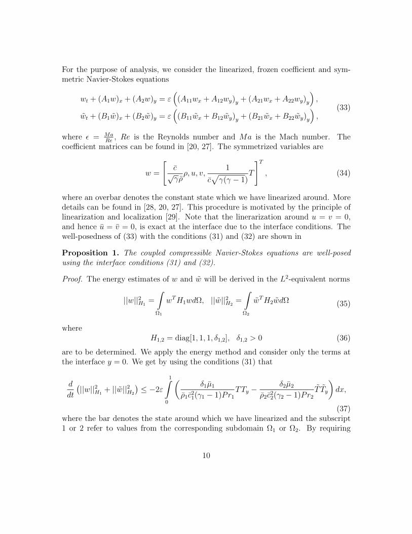
where an overbar denotes the constant state which we have linearized around. Moredetails can be found in [28, 20, 27]. This procedure is motivated by the principle oflinearization and localization [29]. Note that the linerarization around u = v = 0,and hence u = v = 0, is exact at the interface due to the interface conditions. Thewell-posedness of (33) with the conditions (31) and (32) are shown in

Proposition 1. The coupled compressible Navier-Stokes equations are well-posedusing the interface conditions (31) and (32).

Proof. The energy estimates of w and w will be derived in the L2-equivalent norms

||w||2H1=

∫Ω1

wTH1wdΩ, ||w||2H2=

∫Ω2

wTH2wdΩ (35)

whereH1,2 = diag[1, 1, 1, δ1,2], δ1,2 > 0 (36)

are to be determined. We apply the energy method and consider only the terms atthe interface y = 0. We get by using the conditions (31) that

d

dt

(||w||2H1

+ ||w||2H2

)≤ −2ε

1∫0

(δ1µ1

ρ1c21(γ1 − 1)Pr1

TTy −δ2µ2

ρ2c22(γ2 − 1)Pr2

T Ty

)dx,

(37)where the bar denotes the state around which we have linearized and the subscript1 or 2 refer to values from the corresponding subdomain Ω1 or Ω2. By requiring

10

continuity of temperature (T = T ) equation (37) reduces to

d

dt

(||w||2H1

+ ||w||2H2

)≤ −2ε

1∫0

T

(δ1κ1

ρ1c21(γ1 − 1)cP1

Ty −δ2κ2

ρ2c22(γ2 − 1)cP2

Ty

)dx.

(38)In order to obtain an energy estimate by using continuity of the heat fluxes, we needto choose the weights

δ1 = ρ1c21(γ1 − 1)cP1 , δ2 = ρ2c

22(γ2 − 1)cP2 (39)

since then

d

dt

(||w||2H1

+ ||w||2H2

)≤ −2ε

1∫0

T(κ1Ty − κ2Ty

)dx = 0. (40)

Hence the interface conditions (32) gives an energy estimate and no unboundedenergy growth can occur.

Remark 2. The physical interface conditions (32) requires an estimate in a differentnorm than the standard L2-norm. The norm defined by the (positive) weights in(39) is, however, only a scaling of the L2-norm and they are hence equivalent. Froma mathematical point of view, any interface condition which give positive weightswill result in a well-posed coupling.

5.1. The discrete problem and stability

In [12], a stable and conservative multi-block coupling of the Navier-Stokes equa-tions was developed. The coupling was done by considering continuity of all quanti-ties and of the fluxes with the purpose of being able to handle different coordinatetransforms in different blocks. In our case, the velocities are uncoupled and the equa-tions are coupled only by continuity of temperature and heat fluxes. This enable usto compute conjugate heat problems by modifying the interface conditions for themulti-block coupling.

We consider again the formulation (33) and discretize using SBP-SAT for impos-ing the interface conditions (31) and (32) weakly. We let for simplicity the subdo-mains be discretized by equally many uniformly distributed gridpoints which allowus to use the same difference operators in both subdomains. We stress that the sub-domains can have different discretizations [12, 30], this assumption merely simplifiesthe notation and avoids the use of too many subscripts.

11

We discretize (33) using the SBP-SAT technique as

wt + DxF + DyG = S,wt + DxF + DyG = S,

(41)

where the discrete fluxes are given by

F = A1w − ε(A11Dxw + A12Dyw

),

G = A2w − ε(A21Dxw + A22Dyw

),

F = B1w − ε(B11Dxw + B12Dyw

),

G = B2w − ε(B21Dxw + B22Dyw

).

(42)

The hat notation denotes that the matrix has been extended to the entire system as

Dx = Dx ⊗ Iy ⊗ I4, Dy = Ix ⊗Dy ⊗ I4,

Aξ = Ix ⊗ Iy ⊗ Aξ, Bξ = Ix ⊗ Iy ⊗Bξ,(43)

where ξ is a generic index ranging over the indicies which occur in (42).The SATs imposing the interface conditions (31) and (32) can be written as

S = P−1y Ex,yN Σ1

(w − gI

)+ εσ2P

−1y Ex,yN

(H2w − g1

)+ εσ3P

−1y Ex,yN

(H3w − g2

)+ εP−1

y Ex,yN Θ1

(H3Dxw −

∂g2

∂x

)+ εσ4P

−1y Ex,yN

(IT1 w − IT2 w

)+ εσ5P

−1y DT

y Ex,yN

(IT1 w − IT2 w

)+ εσ6P

−1y Ex,yN

(κ1I

T1 Dyw − κ2I

T2 Dyw

)(44)

12

and

S = P−1y Ex,y0Σ2

(w − gI

)+ εσ2P

−1y Ex,y0

(H2w − g1

)+ εσ3P

−1y Ex,y0

(H3w − g2

)+ εP−1

y Ex,y0Θ2

(H3Dxw −

∂g2

∂x

)+ εσ4P

−1y Ex,y0

(IT2 w − IT1 w

)+ εσ5P

−1y DT

y Ex,y0

(IT2 w − IT1 w

)+ εσ6P

−1y Ex,y0

(κ2I

T2 Dyw − κ1I

T1 Dyw

).

(45)

Here P = P⊗I4, Ex,y0 = Ex,y0⊗I4, Hj = Ix⊗Iy⊗Hj and Hj is a 4×4 matrix with theonly non-zero element 1 at the (j, j)th position on the diagonal and the operatorsI1,2 selects the interface elements. The penalty matrices Σ1,2 = Ix ⊗ Iy ⊗ Σ1,2,

Θ1,2 = Ix⊗Iy⊗Θ1,2, and the penalty coefficients σ2,...,6 and σ2,...,6 has to be determinedsuch that the scheme is stable.

Remark 3. The terms which involve Θ1,2 originate from the fact that the boundarycondition v = 0 implies that vx = 0, which is used to obtain an energy estimatein the continuous case. The terms hence represent the artificial boundary conditionvx = 0 which is needed to obtain an energy estimate in the discrete case.

Remember that in the energy estimates for the continuous coupling, a non-standard L2-equivalent norm was used. The same modification to the norms hasto be done in the discrete case. Thus, the discrete energy estimates will be derivedin the norms

||w||2J1

= wT P J1w, ||w||2J2 = wT P J2w, (46)

where,J1 = Ix ⊗ Iy ⊗H1, J2 = Ix ⊗ Iy ⊗H2, (47)

and the matrices H1,2 are defined in (36) with the weights given in (39). Note that

P J1,2 = J1,2P .By applying the energy method to (41) and adding up we get

d

dt||w||2

J1+d

dt||w||2

J2+DI = IT (48)

13

where the dissipation term, DI, is given by

DI = 2ε

[Dxw

Dyw

]T [P J1 0

0 P J1

] [A11 A12

A21 A22

] [Dxw

Dyw

]+ 2ε

[Dxw

Dyw

]T [P J2 0

0 P J2

] [B11 B12

B21 B22

] [Dxw

Dyw

].

(49)

The interface terms can be split into three parts as IT = IT1 + IT2 + IT3 where IT1

are the inviscid terms, IT2 the velocity terms and IT3 the coupling terms related tothe temperature.

In [26] it is shown how to choose Σ1,2, Θ1,2, σ2,3 and σ2,3, with small modifications,such that the inviscid and velocity terms are bounded. Here we focus on the couplingterms. With appropriate choices of Σ1,2, Θ1,2, σ2,3 and σ2,3 as described in [26] weget

d

dt||w||2H1

+d

dt||w||2H2

+DI ≤ IT3, (50)

where IT3 can be written as the quadratic form

IT3 = −ε(Rξ)T (Px ⊗M)Rξ. (51)

To obtain (51), we have used the permutation similarity property of the Kroneckerproduct, R is a permutation matrix and ξ = [Ti, Ti, (DyT)i, (DyT)i]

T where thesubscript i denotes the values at the interface. Note that we do not need the specificform of R, it is sufficient to know that such a matrix exists. Furthermore, we have

Px = diag[δ1Px, δ2Px, δ1Px, δ2Px], (52)

with δ1,2 from (39), and

M =

−2σ4 σ4 + σ4 κ1γ1 − σ5 − κ1σ6 κ2σ6 + σ5

σ4 + σ4 −2σ4 σ5 + κ1σ6 −κ2γ1 − σ5 − κ2σ6

κ1γ1 − σ5 − κ1σ6 σ5 + κ1σ6 0 0κ2σ6 + σ5 −κ2γ1 − σ5 − κ2σ6 0 0

.(53)

Since Px is positive definite and the Kronecker product preserves positive definite-ness, the necessary requirement for (50) to be bounded is that the penalty coefficientsare chosen such that M ≥ 0. The penalty coefficients are given in

14

Theorem 1. The coupling terms IT3 in (50) are bounded using

σ4 = σ4 ≤ 0, σ5 = −κ1r, σ6 = γ + r, σ5 = −κ2(γ1 + r), σ6 = r, r ∈ R (54)

and hence the scheme (41) is stable.

Proof. With the choices of penalty coefficients given in Proposition 1, the matrix Min (53) reduces to

M = 2σ4

−1 1 0 01 −1 0 00 0 0 00 0 0 0

(55)

with eigenvalues λ1,2,3 = 0 and λ4 = −4σ4. Hence if σ4 ≤ 0 we have M ≥ 0.

6. Numerical results

To verify the numerical scheme we use what is often called the method of man-ufactured solutions [4, 31]. We chose the solution and use that to compute a right-hand-side forcing function, initial- and boundary data. According to the principle ofDuhamel [32], the number or form of the boundary conditions does not change dueto the addition of the forcing function. We can hence test the convergence of thescheme towards this analytical solution. The interface conditions (32) are of coursenot satisfied in general by this solution and we need to modify them by adding aright-hand-side.

We use the manufactured solution

ρ(x, y, t) = 1 + η sin(θπ(x− y)− t)2

u(x, y, t) = η cos(θπ(x+ y)− t)v(x, y, t) = η sin(θπ(x− y)− t)p(x, y, t) = 1 + η cos(θπ(x+ y)− t)2,

(56)

with different values of η, θ in the fluid and solid domains, to generate the solution.The energy and temperature can be computed using (11) and (12). Since the stabilityof the scheme is independent of the order of accuracy, the difference operators is theonly thing which have to be changed in order to achieve higher, or lower, accuracy.The rate of convergence, Q, is computed as

Q(j) =1

log(Ni+1

Ni

) log

(E

(j)i

E(j)i+1

)(57)

15

for each of the conserved varables q(j), j = 1, 2, 3, 4. We have used the same numberof grid points, N , in both coordinate directions for both the fluid and solid domain.Nk denotes the number of gridpoints at refinement level k and E

(j)k is the L2-error

between the computed and exact solution for each conserved variable. The timeintegration is done with the classical 4th-order Runge-Kutta method until time t =0.1 using 1000 time steps.

In Table 1 we list the convergence results for the conserved variables for boththe fluid and solid domains. As we can see from Table 1 we can achieve 5th-orderaccuracy by simply replacing the difference operators. No other modifications to thescheme is necessary.

Table 1: Convergence results for the conjugate heat transfer problem

2nd-order 3rd-orderN 32/64 64/96 96/128 32/64 64/96 96/128ρ 1.8367 1.8931 2.0133 2.6222 3.0699 3.4795ρu 2.0824 2.0803 2.1187 2.9846 3.0748 3.1927ρv 2.0503 2.0549 2.0922 3.4222 3.7512 3.4199e 1.8174 1.9065 1.9963 2.4639 2.7749 3.0523ρ 1.8933 1.8533 1.9628 2.5761 2.9791 3.5767ρu 2.0544 2.0803 2.0992 3.1094 3.0374 3.2732ρv 1.9411 2.0190 2.0894 3.3928 3.7465 3.3628e 1.9483 1.9151 1.9409 2.9451 2.8399 3.2560

4th-order 5th-orderN 32/64 64/96 96/128 32/64 64/96 96/128ρ 3.9662 4.1381 4.1138 4.4824 5.2584 5.5131ρu 4.4531 4.3640 4.2799 4.6819 4.7521 4.6733ρv 4.3175 4.0918 4.0284 4.9824 4.9257 4.7839e 3.9757 4.1723 4.0957 4.3760 4.6227 4.7207ρ 3.9935 4.3902 4.5538 4.4421 5.1497 5.5388ρu 4.2072 4.3159 4.4366 4.9665 4.9739 4.9512ρv 4.3672 4.3331 4.3212 5.1007 5.1370 4.9087e 3.9025 4.3178 4.4091 4.8746 4.8573 4.9518

6.1. Comparison of the different approaches to the conjugate heat transfer problem

When the heat transfer in the solid is governed by the compressible Navier-Stokesequations, one does not solve the same conjugate heat transfer problem as when theheat transfer is governed by the heat equation. This is because the relations in (21)

16

holds only approximately as time passes. The exchange of heat between the fluid andsolid domains will affect the temperature and hence also the density, because of theequation of state, and introduce small density variations in the solid domain. We cannumerically solve the conjugate heat transfer problem in both ways and determinethe difference between the two methods. Note that we do not overwrite, or enforce,the velocities to zero inside the solid domain. The velocities are weakly enforced tozero at the boundaries and interfaces only.

Let NS-NS denote the case when the heat transfer is governed by the compressibleNavier-Stokes equations and NS-HT the case where the heat transfer is governed bythe heat equation. The well-posedness and stability of NS-HT coupling is proven inthe appendix. The initial and boundary data are chosen such that NS-NS and NS-HT have identical solutions initially, and we study the differences of the two methodsover time.

To quantify the difference between the two methods, NS-NS and NS-HT, wecompute two representative cases. The computational domain is Ω = Ω1 ∪Ω2 whereΩ1 = [0, 1]×[0, 1] and Ω2 = [0, 1]×[−1, 0]. All computations are done using 3rd-orderaccurate SBP operators and the time integration is done using the classical 4th-orderRunge-Kutta method.

In the first case, the computations are initialized with zero velocities everywhereand temperature T = 1 in both subdomains. In the x-direction we have chosenperiodic boundary conditions. At y = −1 we specify T = 1.5 and at y = 1 we haveT = 1. For the Navier-Stokes equations we have no-slip solid walls as described in[26] for the velocities. These choices of boundary conditions renders the solution tobe homogeneous in the x-direction.

Under the assumption of identically zero velocities and periodicity in the x-direction, the exact steady-state solution can be obtained as

T = − k

2(k + 1)y +

3k + 2

2(k + 1),

T = − 1

2(k + 1)y +

3k + 2

2(k + 1),

(58)

where k = κ2/κ1 is the ratio of the steady-state thermal conductivities. We cansee from (58) that the only occurring material parameter is the ratio between thethermal conductivity coefficients. Neither the density nor the thermal diffusivityhas any effect on the steady-state solution. The larger the ratio of the thermalconductivities is, the stiffer the problem becomes. In the calculations below, we havechosen the parameters such that k = 5.

17

The temperature distribution at time t = 500, which is the steady-state solution,is seen in Figure 1 when using 65 grid points in each coordinate direction and sub-domain. In Figure 2 we show an intersection of the absolute difference along the line−1 ≤ y ≤ 1 at x = 0.5 together with the time-evolution of the l∞- and l2-differences.In Figure 2(b) we can see that the large initial discontinuity gives differences in thebeginning of the computation. As the velocities are damped over time, the differencedecreases rapidly towards zero.

0 0.5 1

−1

−0.8

−0.6

−0.4

−0.2

0

0.2

0.4

0.6

0.8

1

x

y

NS−NS, time t = 500.00, Nx=64, Ny=64

1.05

1.1

1.15

1.2

1.25

1.3

1.35

1.4

1.45

1.5

(a) Temperature distribution from NS-NS

−1 −0.5 0 0.5 11

1.1

1.2

1.3

1.4

1.5

1.6

1.7

1.8

y

Tem

pera

ture

t=500.00, N=64

NS−NS

NS−H

(b) Intersection along y at x = 0.5 of the tem-perature distribution for NS-NS and NS-HT

Figure 1: Temperatures at time t = 500 from NS-NS and NS-HT using 65 grid points in eachcoordinate direction and subdomain

18

−1 −0.5 0 0.5 10

1

2

x 10−4

y

Diffe

rence

t=500.00, N=64

(a) Intersection along y at x = 0.5 of the abso-lute difference in temperature distribution be-tween NS-NS and NS-HT

0 100 200 300 400 5000

0.01

0.02

0.03

0.04

0.05

0.06

0.07

t

Max

Mean

(b) l∞- and l2-difference in time

Figure 2: Temperature intersection and time differences for NS-NS and NS-HT using 65 grid pointsin each coordinate direction and subdomain

In Table 2 we list the results for different number of grid points.

Table 2: Difference between NS-NS and NS-HT at time t = 500Difference

N l∞ l2 Interface32 1.1514e-03 6.8992e-04 1.1514e-0364 2.4612e-04 1.4491e-04 2.4612e-04128 4.3440e-05 2.5329e-05 4.3440e-05

As we can see from Table 2, the differences are very small. Even for the coarsestmesh, the relative maximum and interface differences are less than 0.1% while therelative l2-difference is approximately 0.05%. Note that the differences are decreasingwith the resolution. The steady-state solutions will become identical as the mesh isfurther refined.

Next, we consider an unsteady problem. The boundary data at the south bound-ary is perturbed by the time-dependent perturbation

f(x, t) = 1 + 0.25 ∗ sin(t) ∗ sin(πx) (59)

and hence there will be no steady-state solution. In the x-direction in the soliddomain, we have changed from periodic boundary conditions to solid wall boundary

19

conditions with prescribed temperature T = 1. This is a more realistic way to enclosethe solid domain, and it has the additional benefit of damping the induced velocitiesin the Navier-Stokes equations.

The results can be seen in Figure (3). We plot the l∞- and l2-difference as afunction of time. As we can see, the difference does not approach zero but remainsbounded and small. The relative mean difference is less than 0.5% while the max-imum difference is less than 1.5%. Thus, despite the rather large variation in theboundary data, NS-NS and NS-HT produces very similar solutions.

0 20 40 60 80 1000

0.005

0.01

0.015

0.02

t

Max

Mean

Figure 3: l∞- and l2-difference in time between NS-HS and NS-HT for an unsteady problem

In a CFD computation, the part of the domain which is solid is in general smallcompared to the fluid domain, for example when computing the flow field aroundan airfoil or aircraft. Despite the Navier-Stokes equations being significantly moreexpensive to solve, the overall additional cost of solving the Navier-Stokes equationsalso in the solid is in general limited.

6.2. A numerical example of conjugate heat transfer

As a final computational example, we consider the coupling of a flow over a slabof material for which the ratio of the thermal conductivities is 100. The initialtemperature condition is T = 1 in the fluid domain and T = 1.5 in the solid domain.The boundary conditions are periodic in the x-direction. At the south boundary,y = −1, in the solid domain we let T = 1.5 and at the north boundary, y = 1, inthe fluid domain, there is a Mach 0.5 free-stream boundary condition with T = 1,as described in [28]. Figure 4 shows a snapshot of the solution at time t = 2.5. Thevelocity components in the solid domain are zero to machine precision and the heattransfer in the solid is exclusively driven by diffusion.

20

−0.5 0 0.5 1 1.5−1

−0.8

−0.6

−0.4

−0.2

0

0.2

0.4

0.6

0.8

1

x

yTemperature and velocity field

1.05

1.1

1.15

1.2

1.25

1.3

1.35

1.4

1.45

(a) Temperature distribution and velocity profile

−1 −0.8 −0.6 −0.4 −0.2 0 0.2 0.4 0.6 0.8 1

0.5

1

1.5

2

y

Temperature intersection

Fluid

Solid

(b) Intersection of the temperature distri-bution along x = 0.5.

Figure 4: Temperature and velocity profiles for a flow past a slab of material using 65x65 gridpoints in both domains

7. Conclusions

We have proven that a conjugate heat transfer coupling of the compressibleNavier-Stokes equations is well-posed when a modified norm is used. The equa-tions were discretized using a finite difference method on summation-by-parts formwith boundary- and interface conditions imposed weakly by the simultaneous ap-proximation term. It was shown that a modified discrete norm was needed in orderto prove energy stability of the scheme. The stability is independent of the orderof accuracy, and it was shown that we can achieve all orders of accuracy by simplyusing higher order accurate SBP operators.

We showed that the difference when the heat transfer is governed by the heatequation, compared to the compressible Navier-Stokes equations, is small. Thesteady-state solutions differed by less than 0.005% as the mesh was refined whilea perturbed, unsteady solution differed by less than 0.5% on average.

There are many multi-block codes for the compressible Navier-Stokes equationsavailable. To implement conjugate heat transfer is significantly easier with themethod of modifying the interface conditions, rather than coupling to a differentphysics solver for the heat transfer part. While the Navier-Stokes equations aremore expensive to solve, usually only a small part of the computational domain issolid and the heat transfer is computed at a low additional cost.

21

Acknowledgments

The computations were performed on resources provided by SNIC through Upp-sala Multidisciplinary Center for Advanced Computational Science (UPPMAX) un-der Project p2010056.

Appendix A. Coupling of the compressible Navier-Stokes equations withthe heat equation

In [4], a model problem for conjugate heat transfer was considered. The equationswere one-dimensional, linear and symmetric. In this appendix we extend the work tothe two-dimensional compressible, non-linear Navier-Stokes equations coupled withthe heat equation in two space dimensions. The well-posedness of the coupling isshown in

Proposition 2. The compressible Navier-Stokes equations coupled with the heatequation, is well-posed with the interface conditions

T = T , κTy = κsTy (A.1)

for the temperature, and the no-slip1 conditions

u = 0, v = 0 (A.2)

for the velocities.

Proof. Consider the heat equation (15) and the Navier-Stokes equations in the con-stant, linear, symmetric formulation. The estimates of w and T will be derived inthe L2-equivalent norms

||w||2J1 =

∫Ω1

wTJ1wdΩ1, ||T ||2ν2 =

∫Ω2

T 2ν2dΩ2 (A.3)

where J1 = diag[1, 1, 1, ν1] and ν1,2 > 0 are to be determined.Remember that the symmetrized variables for the Navier-Stokes equations are

w =

[c√γρρ, u, v,

1

c√γ(γ − 1)

T

]T. (A.4)

1See [26] for more general conditions.

22

and note that there is a scaling coefficient in the temperature component. To simplifythe analysis, we rescale (15) by multiplying the equation with 1

c√γ(γ−1

. To apply the

energy method, we rewrite the speed of sound based Peclet number Pec in (14) as

Pec =Pr ·ReMa

=Pr

ε(A.5)

where Pr is the Prandtl number. Then (15) becomes

Tt

c√γ(γ − 1)

=εκs

Prc√γ(γ − 1)ρscs

(Txx + Tyy

). (A.6)

By applying the energy method to each equation and adding the results we obtain

d

dt

(||w||2J1 +

1

c2γ(γ − 1)||T ||2ν2

)≤ −2ε

c2γ(γ − 1)Pr

1∫0

(ν1γµ

ρTTy −

ν2κsρscs

T Ty

)dx.

(A.7)If we choose

ν1 =κρ

γµ, ν2 = ρscs (A.8)

and apply the interface conditions (A.1) we get

d

dt

(||w||2J1 +

1

c2γ(γ − 1)||T ||2ν2

)≤ −2ε

c2γ(γ − 1)Pr

1∫0

T(κTy − κsTy

)dx = 0 (A.9)

and hence the conditions (A.1) does not contribute to unbounded energy growth.

Note again that the application of the physical interface conditions (A.1) requiresthe use of a non-standard norm in the energy estimates. All quantities involved inthe weights ν1,2 are, however, always positive and they will hence always define anorm.

The discretization of the coupled system is analogous to that which is presented in[4], and extended to multiple dimensions as described before. We hence only presentthe numerical scheme and the choice of interface penalty coefficients such that thescheme is stable.

An SBP-SAT discretization of the Navier-Stokes equations coupled with the heat

23

equation is given by, when only considering the interface terms,

wt +(Dx ⊗ I4

)F +

(Dy ⊗ I4

)G = S,

Tt −(D2xT + D2

yT)

= S.(A.10)

The penalty terms are given by

S =(P−1y Ex,yN ⊗ Σ1

) (w − gI

)+ εσ2

(P−1y Ex,yN ⊗ I4

) (H2w − g1

)+ εσ3

(P−1y Ex,yN ⊗ I4

) (H3w − g2

)+ ε

(P−1y Ex,yN ⊗ I4

)Θ1

(H3

(Dx ⊗ I4

)w − ∂g2

∂x

)+ ε

(P−1y Ex,yN ⊗ Σ4

) (IT1 w − IT2 (T⊗ e4)

)+ ε

(P−1y DT

y Ex,yN ⊗ Σ5

) (IT1 w − IT2 (T⊗ e4)

)+ ε

(P−1y Ex,yN ⊗ Σ6

) (κIT1

(Dy ⊗ I4

)w − κsIT2 (DyT⊗ e4)

),

(A.11)

where Σ4,5,6 = diag[0, 0, 0, σ4,5,6] and the term involving Θ1 is explained in Remark 3.The SAT for the heat equation is given by

S = ετ4P−1y Ex,yN

(T−T

)+ ετ5P

−1y DT

y Ex,yN

(T−T

)+ ετ6P

−1y Ex,yN

(κsDyT− κDyT

) (A.12)

and the choices of penalty parameters such that the coupled scheme is stable is givenin

Theorem 2. The scheme (A.10) for coupling the Navier-Stokes equations with theheat equation is stable with the SATs given by (A.11), (A.12) where the penaltycoefficients for the coupling terms are given by

r ∈ R,

σ4 = τ4 ≤ 0, σ5 = −κsr, σ6 =−1 + rPr

Pr, τ5 = − κ (−1 + rPr)

Pr, τ6 = r.

(A.13)

24

Proof. We apply the energy method, using the modified discrete norms,

||w||2J1 = wT (P ⊗ J1)w, ||T||2ν2 = ν2TT PT, (A.14)

where J1 = diag[1, 1, 1, ν1] and ν1,2 are given in (A.8). Using appropriate penaltyterms for the inviscid part and the velocity components of the Navier-Stokes equation,see [33, 26], we obtain the energy estimate

d

dt||w||2J1 +

d

dt||T||2ν2 ≤ 0 (A.15)

when using the penalty coefficients given in (A.13).

References

[1] M. B. Giles. Stability analysis of numerical interface conditions in fluid-structure thermal analysis. International Journal for Numerical Methods inFluids, 25:421–436, August 1997.

[2] B. Roe, R. Jaiman, A. Haselbacher, and P. H. Geubelle. Combined inter-face boundary condition method for coupled thermal simulations. InternationalJournal for Numerical Methods in Fluids, 57:329–354, May 2008.

[3] William D. Henshaw and Kyle K. Chand. A composite grid solver for conju-gate heat transfer in fluid-structure systems. Journal of Computational Physics,228(10):3708–3741, 2009.

[4] Jens Lindstrom and Jan Nordstrom. A stable and high-order accurate conjugateheat transfer problem. Journal of Computational Physics, 229(14):5440–5456,2010.

[5] Michael Schafer and Ilka Teschauer. Numerical simulation of coupled fluid-solid problems. Computer Methods in Applied Mechanics and Engineering,190(28):3645–3667, 2001.

[6] Niphon Wansophark, Atipong Malatip, and Pramote Dechaumphai. Stream-line upwind finite element method for conjugate heat transfer problems. ActaMechanica Sinica, 21:436–443, 2005.

[7] E. Turgeon, D. Pelletier, and F. Ilinca. Compressible heat transfer computa-tions by an adaptive finite element method. International Journal of ThermalSciences, 41(8):721–736, 2002.

25

[8] Xi Chen and Peng Han. A note on the solution of conjugate heat transferproblems using simple-like algorithms. International Journal of Heat and FluidFlow, 21(4):463–467, 2000.

[9] Magnus Svard, Ken Mattsson, and Jan Nordstrom. Steady-state computationsusing summation-by-parts operators. Journal of Scientific Computing, 24(1):79–95, 2005.

[10] Ken Mattsson, Magnus Svard, Mark Carpenter, and Jan Nordstrom. High-order accurate computations for unsteady aerodynamics. Computers and Fluids,36(3):636–649, 2007.

[11] X. Huan, Jason E. Hicken, and David W. Zingg. Interface and boundary schemesfor high-order methods. In the 39th AIAA Fluid Dynamics Conference, AIAAPaper No. 2009-3658, San Antonio, USA, 22-25 June 2009.

[12] Jan Nordstrom, Jing Gong, Edwin van der Weide, and Magnus Svard. A stableand conservative high order multi-block method for the compressible Navier-Stokes equations. Journal of Computational Physics, 228(24):9020–9035, 2009.

[13] Ken Mattsson, Magnus Svard, and Mohammad Shoeybi. Stable and accurateschemes for the compressible Navier-Stokes equations. Journal of ComputationalPhysics, 227:2293–2316, February 2008.

[14] Jan Nordstrom, Sofia Eriksson, Craig Law, and Jing Gong. Shock and vortexcalculations using a very high order accurate Euler and Navier-Stokes solver.Journal of Mechanics and MEMS, 1(1):19–26, 2009.

[15] Jan Nordstrom, Frank Ham, Mohammad Shoeybi, Edwin van der Weide, Mag-nus Svard, Ken Mattsson, Gianluca Iaccarino, and Jing Gong. A hybrid methodfor unsteady inviscid fluid flow. Computers & Fluids, 38:875–882, 2009.

[16] Heinz-Otto Kreiss and Godela Scherer. Finite element and finite differencemethods for hyperbolic partial differential equations. In Mathematical Aspectsof Finite Elements in Partial Differential Equations, number 33 in Publ. Math.Res. Center Univ. Wisconsin, pages 195–212. Academic Press, 1974.

[17] Heinz-Otto Kreiss and Godela Scherer. On the existence of energy estimatesfor difference approximations for hyperbolic systems. Technical report, UppsalaUniversity, Division of Scientific Computing, 1977.

26

[18] Mark H. Carpenter, David Gottlieb, and Saul Abarbanel. Time-stable boundaryconditions for finite-difference schemes solving hyperbolic systems: Methodol-ogy and application to high-order compact schemes. Journal of ComputationalPhysics, 111(2):220–236, 1994.

[19] Mark H. Carpenter, Jan Nordstrom, and David Gottlieb. A stable and conserva-tive interface treatment of arbitrary spatial accuracy. Journal of ComputationalPhysics, 148(2):341–365, 1999.

[20] Jan Nordstrom and Magnus Svard. Well-posed boundary conditions for theNavier-Stokes equations. SIAM Journal on Numerical Analysis, 43(3):1231–1255, 2005.

[21] Bo Strand. Summation by parts for finite difference approximations for d/dx.Journal of Computational Physics, 110(1):47–67, 1994.

[22] Ken Mattsson and Jan Nordstrom. Summation by parts operators for finite dif-ference approximations of second derivatives. Journal of Computational Physics,199(2):503–540, 2004.

[23] Ken Mattsson. Summation by parts operators for finite difference approxi-mations of second-derivatives with variable coefficients. Journal of ScientificComputing, pages 1–33, 2011.

[24] Jorg U. Schluter, Xiaohua Wu, Edwin van der Weide, S. Hahn, Juan J. Alonso,and Heinz Pitsch. Multi-code simulations: A generalized coupling approach.In the 17th AIAA CFD Conference, AIAA-2005-4997, Toronto, Canada, June2005.

[25] Magnus Svard and Jan Nordstrom. On the order of accuracy for differenceapproximations of initial-boundary value problems. Journal of ComputationalPhysics, 218(1):333–352, 2006.

[26] Jens Berg and Jan Nordstrom. Stable Robin solid wall boundary conditions forthe Navier-Stokes equations. Journal of Computational Physics, 230(19):7519–7532, 2011.

[27] Saul Abarbanel and David Gottlieb. Optimal time splitting for two- and three-dimensional Navier-Stokes equations with mixed derivatives. Journal of Com-putational Physics, 41(1):1–33, 1981.

27

[28] Magnus Svard, Mark H. Carpenter, and Jan Nordstrom. A stable high-order fi-nite difference scheme for the compressible Navier-Stokes equations, far-fieldboundary conditions. Journal of Computational Physics, 225(1):1020–1038,2007.

[29] Heinz-Otto Kreiss and Jens Lorenz. Initial-Boundary Value Problems and theNavier-Stokes Equations. Classics in Applied Mathematics. Society for Indus-trial and Applied Mathematics, 2004.

[30] Ken Mattsson and Mark H. Carpenter. Stable and accurate interpolation op-erators for high-order multiblock finite difference methods. SIAM Journal onScientific Computing, 32(4):2298–2320, 2010.

[31] Lee Shunn, Frank Ham, and Parviz Moin. Verification of variable-densityflow solvers using manufactured solutions. Journal of Computational Physics,231(9):3801–3827, 2012.

[32] Bertil Gustafsson, Heinz-Otto Kreiss, and Joseph Oliger. Time Dependent Prob-lems and Difference Methods. Wiley Interscience, 1995.

[33] Magnus Svard and Jan Nordstrom. A stable high-order finite difference schemefor the compressible Navier-Stokes equations: No-slip wall boundary conditions.Journal of Computational Physics, 227(10):4805–4824, 2008.

28