Large Eddy Simulation Applied on the Analysis of Vortex Tube · Ranque-Hilsch vortex tube (RHVT). The gas is injected tangentially into a nozzle chamber with high degree of swirl

International Journal of Engineering and Technical Research (IJETR)

ISSN: 2321-0869 (O) 2454-4698 (P), Volume-6, Issue-2, October 2016

49 www.erpublication.org

Abstract— This paper deals with the work carried out in

Ranque-Hilsch vortex tube (RHVT). The gas is injected

tangentially into a nozzle chamber with high degree of swirl

velocity so that air travels in a spiral motion along the periphery

of the hot side. A three dimensional RHVT model is constructed

and used to carry out the numerical computation in the

framework of commercial CFD code Fluent for predicting the

energy separation and flow phenomenon inside the tube.

Moreover, five turbulence models including standard k-epsilon

(sk-ɛ), renormalization group k-epsilon (RNG k-ɛ), k-omega

(k-ω), Reynolds stress model (RSM) and large eddy simulation

(LES) model are adopted in the calculating procedures for

evaluating their outcomes. As a result, the numerical simulations

clearly illustrate the temperature separation and flow

phenomena within the vortex tube. Also, the CFD flow

visualization on vortex tube can identify three regions, which

are the incoming fluid at ambient temperature and high

pressure, the cold exit and the hot exit where the temperatures

are significant lower or higher than the inlet temperature,

respectively. Also, performance curves (cold temperature

separation versus cold outlet mass fraction) of vortex tube were

obtained successfully under a given inlet pressure. Regards the

comparison among turbulent models, CFD predictions from the

large eddy simulation yields the best high-resolution flow

pattern and provides more detailed information for

understanding the physical mechanisms of this flow and energy

separation. Also, its calculated results are in a better agreement

with the available experimental measurements compared to

other turbulent models.

Index Terms— Ranque-Hilsch vortex tube, CFD code Fluent,

sk-ɛ, RNGk-ɛ, k-ω, RSM and LES

I. INTRODUCTION

An external analysis proves that the RHVT obeys both the

First and Second Laws of Thermodynamics. However this

external analysis does not offer any insight into the internal

mechanisms of the RHVT which force the temperature

separations to both the hot and cold outlets. Despite the

simplicity of the vortex tubes geometry, the energy separation

phenomenon within the RHVT is quite complex. At present

several conflicting theories have been advanced to explain the

vortex tubes behavior since its initial observation by Ranque

[1]. He explained Heat supplying process takes place by the

inner sheet of fluid expanding so as to compressing the outer

sheet of fluid. Hilsch [2] designed the vortex tube for better

efficiency and hypothesized the expansion of a gas in a

centrifugal field producing cold gas and heating of gas due to

friction to yield the temperature separation. Scheper [5] found

that the static temperature decreased in a radially outward

direction. He hypothesized the energy separation mechanism

as heat transfer by forced convection. Martynovskii and

Million Asfaw Belay, Lecturer, Bahirdar Institute of Technology,

Bahirdar University,Bahirdar, Ethiopia.

Alekseev [6] obtained the analytic expression for the ratio of

kinetic energy and heat currents and conducted experiment to

verify a hypothesis. They argued that temperature separation

is obtained due to work transfer from core to periphery. Bruun

[7] measured the velocity distribution of air in a counter flow

vortex tube at various cross-sections. Comparison is made

between the order of magnitude of the radial and axial

convection terms in the equations of motion and energy. He

argued that turbulent heat transport could lead to temperature

separation. Yunpeng Xue et al. [8] have shown that the energy

separation in the vortex tube seems to involve a number of

different factors, among which expansion and friction

between the flow layers could be considered as the most

important.

Recently, computational fluid dynamics (CFD) modeling

has been successfully utilized to explain the fundamental

principles behind energy separation. Promvonge [9] used an

algebraic Reynolds stress model (ASM) and the k– ɛ

turbulence model for CFD simulation of the flow phenomena

in a vortex tube. He observed a better prediction of

temperature separation by the ASM over the k– ɛ turbulence

model. Frohlingsdorf and Unger [10] presented a CFD model

of energy separation by considering compressibility and

turbulence effects. They used the CFX code with the k–ɛ

turbulence model. Behera et al. [11] presented a three

dimensional CFD model for analysis of energy separation

using code system STAR CD with the RNG k– ɛ turbulence

model. They investigated the effect of shape, size and number

of nozzles on temperature separation in the vortex tube.

Aljuwayhel et al. [4] investigated the energy separation

mechanism using code system Fluent. They observed that the

standard k– ɛ turbulence model predicted the velocity and

temperature separation better than the RNG k–ɛ turbulence

model. Skye et al. [3] also reported similar results.

Eiamsa-ard and Promvonge [12] used a mathematical model

for the simulation of energy separation effect. They used the

ASM and k–ɛ turbulence model and concluded that the

diffusive transport of mean kinetic energy had a substantial

influence on energy separation. H. Khazaei et al. [14]

demonstrates about energy separation effects in a vortex tube

using a CFD model. The effects of varying the geometry of

vortex tube components, such as hot outlet and diameter size,

on tube performance, have been studied, besides using

different gases as a working medium in a vortex tube. Rahim

Shamsoddini et al. [15], deals on the effects of the nozzles

number on the flow and power of cooling of a vortex tube

using a three-dimensional numerical fluid dynamic model.

They observed that as the number of nozzles increased, power

of cooling increases significantly while cold outlet

temperature decreases moderately. H. Pourariaa et al. [16]

indicated that an increase in divergent tube angle results in an

increase in cooling performance of vortex tube. However,

there is a critical divergence angle, so that further increase

Large Eddy Simulation Applied on the Analysis of

Vortex Tube

Million Asfaw Belay

Large Eddy Simulation Applied on the Analysis of Vortex Tube


will lead to reduction in cooling performance of the device.

Tanvir Farouk et al. [13] used the CFD-ACE+ code to predict

the energy separation. They used the large eddy simulation

(LES) technique to model the turbulence and compared the

predicted results with the published experimental results

(Skye et al.) and k– ɛ predictions. They observed that

temperature separation predicted by the LES was closer to the

experimental results. However, the vortex tube dimensions

and inlet boundary condition used in the LES model are

significantly different from those used in the experiment. Also

they used LES technique for predicting the gas flow and

temperature fields and the species mass fractions (nitrogen

and helium) in the vortex tube. Hence, there should be a

tradeoff between accuracy and computational expenses. If

reasonable accuracy is obtained with a lower order turbulence

model, then it can be used for design purpose the model is

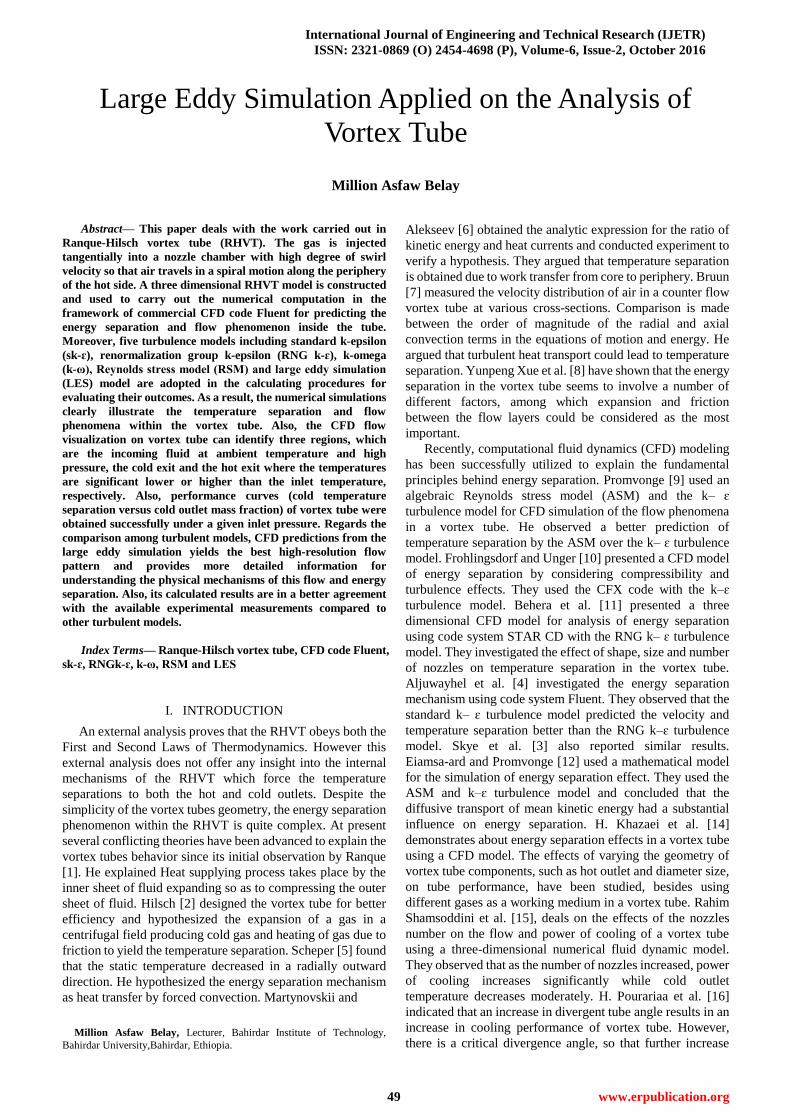
shown in Fig 1.

Fig. 1 The fluid flow inside a vortex tube

From this literature review it is observed that none of the

researchers performed a three dimensional numerical

simulation of vortex tube using LES turbulence model. Thus,

the main motivation of this paper is a three dimensional

vortex tube with a high pressure inlet boundary condition

(400kPa) and a low pressure inlet boundary condition

(200kPa) using different type of CFD models including LES

to compare the fluid flow and temperature separation so that a

computationally less expensive suitable turbulence model can

be chosen for the simulation of vortex tube. The models that

are used in this work are Reynolds average Navier–Stokes

(RANS) based turbulence models (i.e., standard k–ɛ, RNG

k–ɛ and k–ω) and more advanced turbulence models (i.e.,

RSM and LES). The primary and fundamental objectives of

this research work are; to determine a temperature separation

and a fundamental understanding of the fluid dynamics and

thermodynamics of the primary and secondary flows in the

vortex tube, to investigated the performance curve, to

compare and contrast the temperature separation and flow

field along the VT of five turbulence models, to locate the

position of stagnation point and secondary flow in VT, to

identify the major reason for temperature separation and its

mechanism, to study the vortex tube characteristics by

observing the pressure, velocity and temperature fields, and

the results from the turbulence models are analyzed and

compared to establish how accurate they are at computing this

type of flow field.

II. CFD MODELING

2.1. Geometry of Model

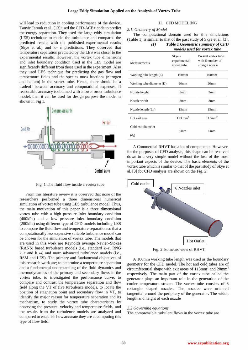
The computational domain used for this simulations

(Table 1) is similar to that of the past study of Skye et al. [3].

(1) Table 1 Geometric summery of CFD

models used for vortex tube

Measurements

Skye's

experimental

vortex tube

Present vortex tube

with 6 number of

straight nozzle

Working tube length (L) 100mm 100mm

Working tube diameter (D) 20mm 20mm

Nozzle height 3mm 3mm

Nozzle width 3mm 3mm

Nozzle length (LN) 15mm 15mm

Hot exit area 113 mm2 113mm2

Cold exit diameter

(dc)

6mm 6mm

A Commercial RHVT has a lot of components. However,

for the purposes of CFD analysis, this shape can be resolved

down to a very simple model without the loss of the most

important aspects of the device. The basic elements of the

vortex tube which is similar to that of the past study of Skye et

al. [3] for CFD analysis are shown on the Fig. 2.

Fig. 2 Isometric view of RHVT

A 100mm working tube length was used as the boundary

geometry for the CFD model. The hot and cold tubes are of

circumferential shape with exit areas of 113mm2 and 28mm

2

respectively. The main part of the vortex tube called the

generator plays an important role in the generation of the

cooler temperature stream. The vortex tube consists of 6

rectangle shaped nozzles. The nozzles were oriented

tangential around the periphery of the generator. The width,

length and height of each nozzle

2.2 Governing equations

The compressible turbulent flows in the vortex tube are

Cold outlet 6 Nozzles inlet

Hot Outlet




governed by;

Conservation of Mass:

(1)

Conservation of Momentum

(2)

Conservation of Energy

(3)

State equation (4)

2.3 Assumptions and Boundary Conditions

Basic assumptions involved for all computational

turbulence models for analysis of vortex-tube are

compressible flow, steady or transient (specifically for LES

turbulence model), turbulent, subsonic three dimension flow

with uniform fluid properties at the inlet. The compressible

fluid is treated as an ideal gas. This paper focused on high and

low pressure inlet boundary conditions for all type of

turbulent models to identify the effects of inlet pressure on the

fluid field and temperature separation. In the inlet region,

pressure boundary condition of the vortex tube with inlet

pressure 400 kPa for high pressure inlet condition and 200

kPa for low pressure inlet condition and a total temperature of

300 K is defined (Table 2). The inlet region consists of 6

nozzles. The hot outlet is considered as circumferential outlet.

In the computational domain as shown in Fig. 2 the air

enters the vortex tube through the nozzles with a tangential

velocity. Pressure outlet is the recommended boundary

condition at outlet for an ideal gas in turbulent flow, which

was adopted in this work at the cold and hot outlets.

Atmospheric pressure was specified at the cold exit of the

vortex tube. The pressure boundary condition at the hot exit

was varied to control the mass flow rates among the two exits

shown at Table 2. The temperature at the hot and cold exits

was assigned a zero gradient boundary condition. The tube

walls were considered to be adiabatic with no slip boundary

condition for the velocity components.

Table 2 Variable and fixed parameters for the vortex tube

simulations

Case

Fixed parameters Variable

parameters

Inlet

pressure

(kPa)

Cold exit

pressure

(kPa)

Hot exit

pressure

(kPa)

1 105

2 60

3 70

4 400 101.325 80

5 90

6 100

7 110

8 115

9 200 101.325 105

2.4 Grid independence study

A mesh convergence study focusing on cold temperature

outputs of the RHVT was conducted. This study was carried

out in order to ascertain a mesh density such that any potential

increase in the number of elements/nodes above the largest

solved mesh density would yield a marginal increase in

accuracy of CFD results, insufficient to warrant any increase

in mesh density. This final mesh density was then used with

confidence for comparative studies of other factors such as

choice of turbulence model and changes the inlet pressure of

the RHVT.

For case 1 with hot exit pressure 105 kPa, grid independence

tests were carried out for several grid designs. Initially the k–ɛ

turbulence model is utilized to perform a mesh element

density convergence study with the cold temperature outputs

of the vortex tube as the measured criteria. The variation of

the key parameters such as the cold temperature difference for

different cell volumes was investigated. Investigations of the

mesh density showed that the model predictions are

insensitive to the number of grids above 500,000 (Fig. 3).

Once mesh independent test is established additional

turbulence models such as the RNG k-ɛ, k-ω and RSM are run

on this mesh to ascertain the performance of each turbulence

model. But LES needs more fined type of mesh than others so

that it has an accurate result with the experiment one.

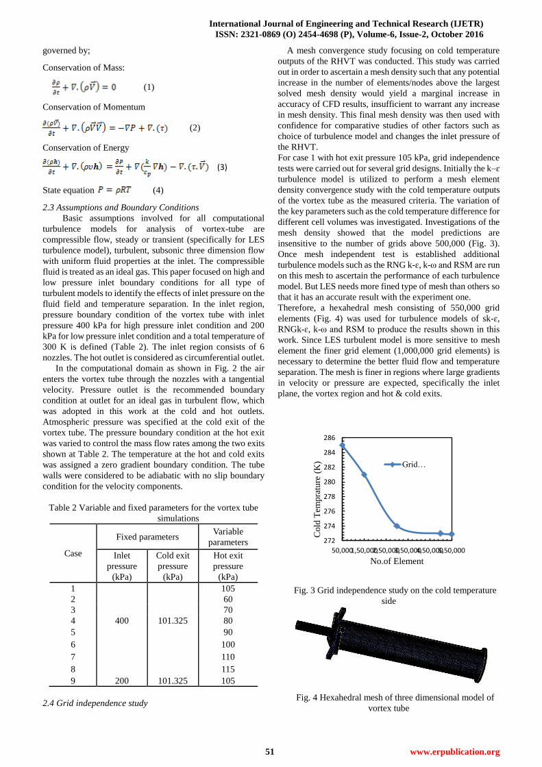
Therefore, a hexahedral mesh consisting of 550,000 grid

elements (Fig. 4) was used for turbulence models of sk-ɛ,

RNGk-ɛ, k-ω and RSM to produce the results shown in this

work. Since LES turbulent model is more sensitive to mesh

element the finer grid element (1,000,000 grid elements) is

necessary to determine the better fluid flow and temperature

separation. The mesh is finer in regions where large gradients

in velocity or pressure are expected, specifically the inlet

plane, the vortex region and hot & cold exits.

272

274

276

278

280

282

284

286

50,0001,50,0002,50,0003,50,0004,50,0005,50,000

Cold

Tem

pra

ture

(K

)

No.of Element

Grid…

Fig. 3 Grid independence study on the cold temperature

side

Fig. 4 Hexahedral mesh of three dimensional model of

vortex tube



2.5 Solution procedures

After successfully accomplished the geometry and mesh

of vortex tube the next step was solving Navier-stokes

equations and energy equations using finite-volume method

(using Fluent code) together with the relevant turbulence

model equations.

For sk-ɛ, RNG k-ɛ, k-ω and RSM the simple algorithm

was selected for pressure-velocity decoupling. The

discretization of the governing equations is accomplished by a

first-order upwind scheme. The air entering the tube is

modeled as an ideal gas of constant specific heat capacity,

thermal conductivity, and viscosity. Due to the highly

non-linear and coupled features of the governing equations

for swirling flows, low under-relaxation factor 0.2 was used

for pressure, momentum, turbulent kinetic energy and energy,

to ensure the stability and convergence. The convergence

criterion for the residual was set as 1x10-5

for all equations.

For transient LES turbulence model simple algorithm are

used for pressure-velocity decoupling. For the

convective–diffusive terms in the mass, momentum and

energy conservation equations a second-order upwind scheme

[17] is used. The Kolmogorov time scale calculated from the

micro scale relations was found to be 2x10-4

s. A 10 µs

time-step size with 50,000 number of time step was chosen,

which is smaller than the Kolmogorov time scale. The implicit

calculations within a given time-step are continued until the

variation in the variables is within 10-05

% of the value of the

variable from the previous iteration. The time marching

calculations were terminated when a pseudo steady-state

behavior was observed.

III. RESULTS AND DISCUSSION

This section focused on the pressure contour, temperature

contour, velocity contour of the vortex tube and the velocity

field at x/L=0.5 of the vortex tube with different turbulence

model. To simplify the study we categories it in to two parts

i.e., for high pressure inlet boundary condition (400 kPa) and

low pressure inlet boundary condition (200 kPa).

3.1 Thermal performance

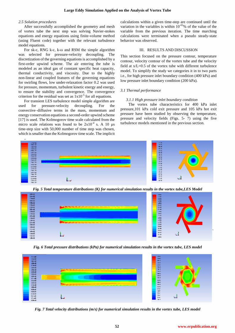
3.1.1 High pressure inlet boundary condition

The vortex tube characteristics for 400 kPa inlet

pressure,101 kPa cold exit pressure and 105 kPa hot exit

pressure have been studied by observing the temperature,

pressure and velocity fields (Figs. 5- 7) using the five

turbulence models mentioned in the previous section.

..

Fig. 5 Total temperature distributions (K) for numerical simulation results in the vortex tube,LES Model

Fig. 6 Total pressure distributions (kPa) for numerical simulation results in the vortex tube, LES model

Fig. 7 Total velocity distributions (m/s) for numerical simulation results in the vortex tube, LES model




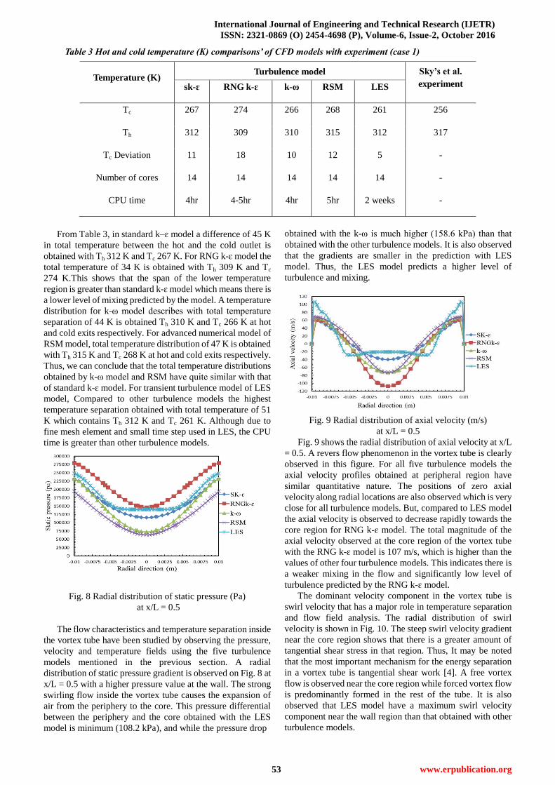
Table 3 Hot and cold temperature (K) comparisons’ of CFD models with experiment (case 1)

Temperature (K) Turbulence model Sky’s et al.

experiment sk-ɛ RNG k-ɛ k-ω RSM LES

Tc 267 274 266 268 261 256

Th 312 309 310 315 312 317

Tc Deviation 11 18 10 12 5 -

Number of cores 14 14 14 14 14 -

CPU time 4hr 4-5hr 4hr 5hr 2 weeks -

From Table 3, in standard k–ɛ model a difference of 45 K

in total temperature between the hot and the cold outlet is

obtained with Th 312 K and Tc 267 K. For RNG k-ɛ model the

total temperature of 34 K is obtained with Th 309 K and Tc

274 K.This shows that the span of the lower temperature

region is greater than standard k-ɛ model which means there is

a lower level of mixing predicted by the model. A temperature

distribution for k-ω model describes with total temperature

separation of 44 K is obtained Th 310 K and Tc 266 K at hot

and cold exits respectively. For advanced numerical model of

RSM model, total temperature distribution of 47 K is obtained

with Th 315 K and Tc 268 K at hot and cold exits respectively.

Thus, we can conclude that the total temperature distributions

obtained by k-ω model and RSM have quite similar with that

of standard k-ɛ model. For transient turbulence model of LES

model, Compared to other turbulence models the highest

temperature separation obtained with total temperature of 51

K which contains Th 312 K and Tc 261 K. Although due to

fine mesh element and small time step used in LES, the CPU

time is greater than other turbulence models.

Fig. 8 Radial distribution of static pressure (Pa)

at x/L = 0.5

The flow characteristics and temperature separation inside

the vortex tube have been studied by observing the pressure,

velocity and temperature fields using the five turbulence

models mentioned in the previous section. A radial

distribution of static pressure gradient is observed on Fig. 8 at

x/L = 0.5 with a higher pressure value at the wall. The strong

swirling flow inside the vortex tube causes the expansion of

air from the periphery to the core. This pressure differential

between the periphery and the core obtained with the LES

model is minimum (108.2 kPa), and while the pressure drop

obtained with the k-ω is much higher (158.6 kPa) than that

obtained with the other turbulence models. It is also observed

that the gradients are smaller in the prediction with LES

model. Thus, the LES model predicts a higher level of

turbulence and mixing.

Fig. 9 Radial distribution of axial velocity (m/s)

at x/L = 0.5

Fig. 9 shows the radial distribution of axial velocity at x/L

= 0.5. A revers flow phenomenon in the vortex tube is clearly

observed in this figure. For all five turbulence models the

axial velocity profiles obtained at peripheral region have

similar quantitative nature. The positions of zero axial

velocity along radial locations are also observed which is very

close for all turbulence models. But, compared to LES model

the axial velocity is observed to decrease rapidly towards the

core region for RNG k-ɛ model. The total magnitude of the

axial velocity observed at the core region of the vortex tube

with the RNG k-ɛ model is 107 m/s, which is higher than the

values of other four turbulence models. This indicates there is

a weaker mixing in the flow and significantly low level of

turbulence predicted by the RNG k-ɛ model.

The dominant velocity component in the vortex tube is

swirl velocity that has a major role in temperature separation

and flow field analysis. The radial distribution of swirl

velocity is shown in Fig. 10. The steep swirl velocity gradient

near the core region shows that there is a greater amount of

tangential shear stress in that region. Thus, It may be noted

that the most important mechanism for the energy separation

in a vortex tube is tangential shear work [4]. A free vortex

flow is observed near the core region while forced vortex flow

is predominantly formed in the rest of the tube. It is also

observed that LES model have a maximum swirl velocity

component near the wall region than that obtained with other

turbulence models.

../../../Documents%20and%20Settings/Users/Million/Desktop/Thesis/Final-Million-thesis.doc#_ENREF_12



Figure 11 shows the radial distribution of radial velocity at

x/L = 0.5. The magnitude of the radial velocity component is

much smaller compared to the other components. A negative

value of the radial velocity means the flow direction in the

vortex tube is radially inward. For RNG k-ɛ model a radial

velocity component profile has a significant deviation near

the core region compared to other turbulence models. This

may indicate that there is lower level of turbulence predicted

by the RNG k-ɛ model near the core region.

Fig. 10 Radial distribution of swirl velocity (m/s)

at x/L = 0.5

Fig. 11 Radial distribution of radial velocity (m/s)

at x/L = 0.5

Figure 12 shows the radial distribution of static

temperature at x/L = 0.5. It observed the Static temperature is

decrease sharply near to the periphery boundary layer

followed by fairly constant with radial direction. Aljuwayhel

et al.[4] also stated similar thing regarding to static

temperature distribution. As it observed from Fig. 12 for all

turbulence models the static temperature profiles have similar

qualitative nature, the static temperatures at the periphery and

the core region and the static temperature differentials

between the periphery and the core are observed to be

considerably different.

Fig. 12 Radial distribution of static temperature (K)

at x/L = 0.5

The static temperature differentials between the periphery

and the core predicted by RNG k-ɛ model, k-ω model, RSM

model, and LES model are 28 K, 28.6 K, 32 and 46.9,

respectively, which are higher than standard k-ɛ model with

value of 23.7 K. These differentials for different turbulence

models have contribution for variation in the pressure

gradient between the periphery and the core with in these

turbulence models which have a big role on the level of

turbulent mixing (Fig. 8).

It has been observed that the greater temperature

differential is due to the higher pressure drop. Also, lower the

static pressure at the core region would cause for lower static

temperature at that location. So, it concludes that the static

temperature drop can be described as a result of the radial

expansion of air in the vortex tube.

The radial distribution of total temperature at x/L = 0.5 is

presented in Fig. 13. The total temperature profiles is the sum

of the constant static pressure profiles (Fig. 8) and swirl

velocity (tangential velocity) profiles (Fig. 10). Static

temperature is calculated from static enthalpy while total

temperature is outcomes from total enthalpy, which consists

of both kinetic energy and static enthalpy.

The dominancy of strongly swirling flow inside the vortex

tube causes the expansion of air from the periphery to the core

region, which causes for reducing the static pressure and static

temperature near the core. Generally the distribution of static

pressure is determined by the distribution of static

temperature while the swirl velocity component, determines

the distribution of the kinetic energy and total enthalpy inside

the vortex tube.

Fig. 13 Radial distribution of total temperature (K)

Basically the total temperature profile follows the swirl

velocity profile since the static temperature is fairly constant

in the radial direction except near the wall. Thus, consistency

of the total temperature profile with the profiles of static

pressure and swirl velocity indicates that the temperature

separation between the peripheral and inner fluid layers is due

to a combination of the radial expansion of air and the change

in kinetic energy. Due to the shear work done by the inner

fluid layers on the peripheral layers, fluid in the core region

possesses lower kinetic energy, thereby lowering the total

enthalpy and total temperature.

Although all turbulence models have similar qualitative

nature of the total temperature profiles, the total temperatures

at the periphery and the core and the total temperature

differential between them have different quantitative value for

each of these turbulence models. The total temperature

differential between the periphery and the core region

obtained with the LES model (48.8 K) is relatively higher than

other turbulence models. This variation with different





turbulence models have a big contribution to the variation in

the levels of turbulence predicted by the models.

Fig. 14 Cold exit temperature separation (T in – Tc) as

a function of cold mass fraction

The temperature separation obtained from the present

standard k-ɛ, Farouk et.al. LES and 3-D LES calculations

were compared with experimental result of Skye et al [3] for

validation. As seen in Fig. 14, the cold exit temperature

separations predicted by the models are in good agreement

with the experimental results. Also we conclude that the cold

temperature separation calculated by LES turbulent model of

3-D VT is better than other models shown on Fig. 14. The

cold exit temperature difference is observed to decrease with

an increase in the cold mass fraction. Thus the maximum cold

temperature difference was observed in the cold mass fraction

range of 0.2 to 0.4

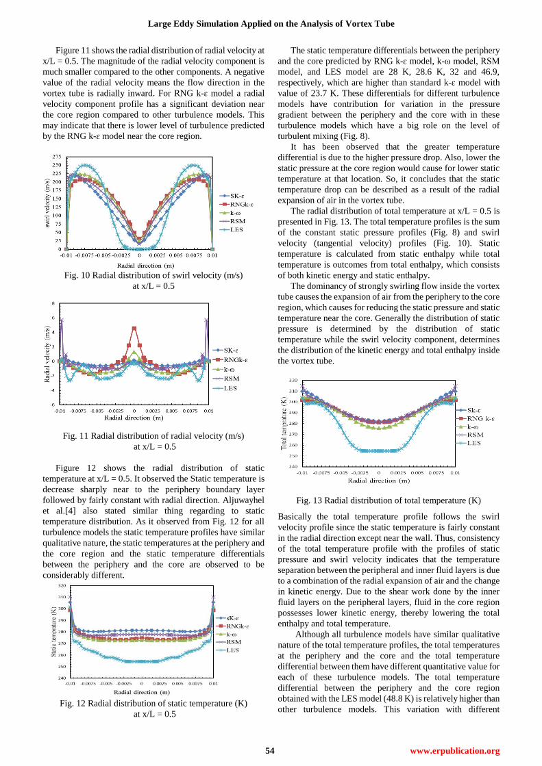
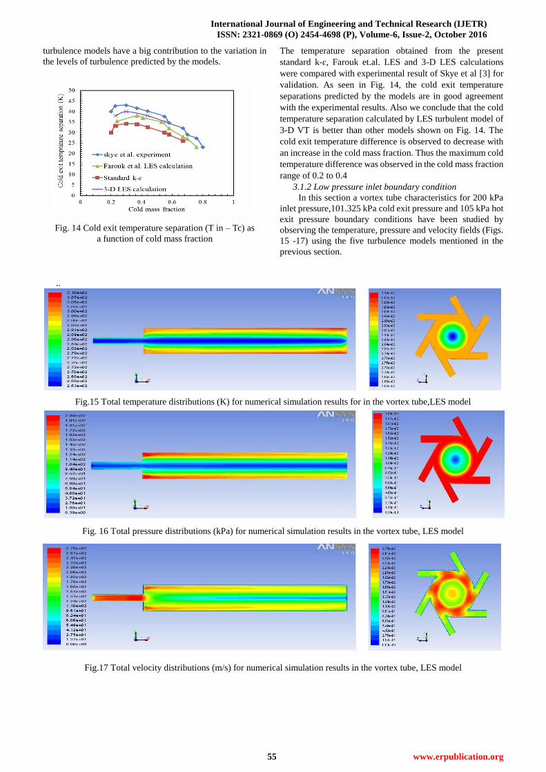
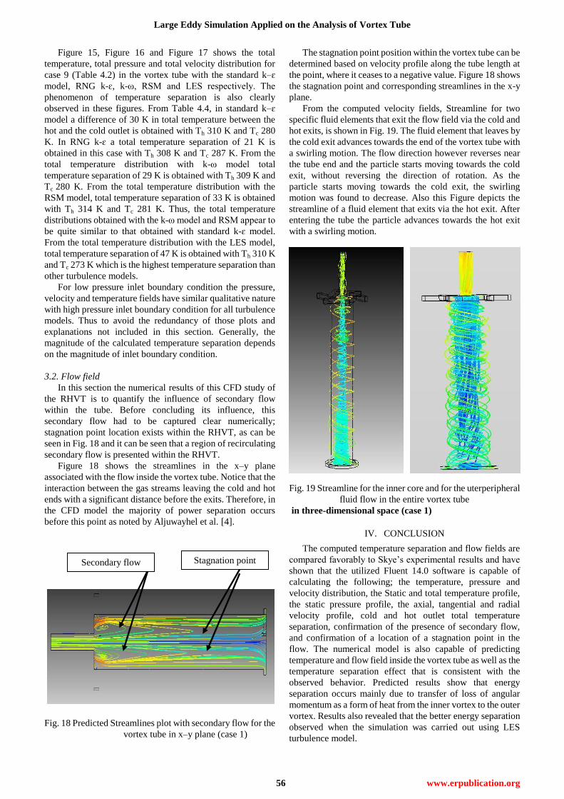
3.1.2 Low pressure inlet boundary condition

In this section a vortex tube characteristics for 200 kPa

inlet pressure,101.325 kPa cold exit pressure and 105 kPa hot

exit pressure boundary conditions have been studied by

observing the temperature, pressure and velocity fields (Figs.

15 -17) using the five turbulence models mentioned in the

previous section.

..

Fig.15 Total temperature distributions (K) for numerical simulation results for in the vortex tube,LES model

Fig. 16 Total pressure distributions (kPa) for numerical simulation results in the vortex tube, LES model

Fig.17 Total velocity distributions (m/s) for numerical simulation results in the vortex tube, LES model




Figure 15, Figure 16 and Figure 17 shows the total

temperature, total pressure and total velocity distribution for

case 9 (Table 4.2) in the vortex tube with the standard k–ɛ

model, RNG k-ɛ, k-ω, RSM and LES respectively. The

phenomenon of temperature separation is also clearly

observed in these figures. From Table 4.4, in standard k–ɛ

model a difference of 30 K in total temperature between the

hot and the cold outlet is obtained with Th 310 K and Tc 280

K. In RNG k-ɛ a total temperature separation of 21 K is

obtained in this case with Th 308 K and Tc 287 K. From the

total temperature distribution with k-ω model total

temperature separation of 29 K is obtained with Th 309 K and

Tc 280 K. From the total temperature distribution with the

RSM model, total temperature separation of 33 K is obtained

with Th 314 K and Tc 281 K. Thus, the total temperature

distributions obtained with the k-ω model and RSM appear to

be quite similar to that obtained with standard k-ɛ model.

From the total temperature distribution with the LES model,

total temperature separation of 47 K is obtained with Th 310 K

and Tc 273 K which is the highest temperature separation than

other turbulence models.

For low pressure inlet boundary condition the pressure,

velocity and temperature fields have similar qualitative nature

with high pressure inlet boundary condition for all turbulence

models. Thus to avoid the redundancy of those plots and

explanations not included in this section. Generally, the

magnitude of the calculated temperature separation depends

on the magnitude of inlet boundary condition.

3.2. Flow field

In this section the numerical results of this CFD study of

the RHVT is to quantify the influence of secondary flow

within the tube. Before concluding its influence, this

secondary flow had to be captured clear numerically;

stagnation point location exists within the RHVT, as can be

seen in Fig. 18 and it can be seen that a region of recirculating

secondary flow is presented within the RHVT.

Figure 18 shows the streamlines in the x–y plane

associated with the flow inside the vortex tube. Notice that the

interaction between the gas streams leaving the cold and hot

ends with a significant distance before the exits. Therefore, in

the CFD model the majority of power separation occurs

before this point as noted by Aljuwayhel et al. [4].

Fig. 18 Predicted Streamlines plot with secondary flow for the

vortex tube in x–y plane (case 1)

The stagnation point position within the vortex tube can be

determined based on velocity profile along the tube length at

the point, where it ceases to a negative value. Figure 18 shows

the stagnation point and corresponding streamlines in the x-y

plane.

From the computed velocity fields, Streamline for two

specific fluid elements that exit the flow field via the cold and

hot exits, is shown in Fig. 19. The fluid element that leaves by

the cold exit advances towards the end of the vortex tube with

a swirling motion. The flow direction however reverses near

the tube end and the particle starts moving towards the cold

exit, without reversing the direction of rotation. As the

particle starts moving towards the cold exit, the swirling

motion was found to decrease. Also this Figure depicts the

streamline of a fluid element that exits via the hot exit. After

entering the tube the particle advances towards the hot exit

with a swirling motion.

Fig. 19 Streamline for the inner core and for the uterperipheral

fluid flow in the entire vortex tube

in three-dimensional space (case 1)

IV. CONCLUSION

The computed temperature separation and flow fields are

compared favorably to Skye’s experimental results and have

shown that the utilized Fluent 14.0 software is capable of

calculating the following; the temperature, pressure and

velocity distribution, the Static and total temperature profile,

the static pressure profile, the axial, tangential and radial

velocity profile, cold and hot outlet total temperature

separation, confirmation of the presence of secondary flow,

and confirmation of a location of a stagnation point in the

flow. The numerical model is also capable of predicting

temperature and flow field inside the vortex tube as well as the

temperature separation effect that is consistent with the

observed behavior. Predicted results show that energy

separation occurs mainly due to transfer of loss of angular

momentum as a form of heat from the inner vortex to the outer

vortex. Results also revealed that the better energy separation

observed when the simulation was carried out using LES

turbulence model.

Secondary flow Stagnation point





REFERENCES

[1] G. Ranque, Experiments on expansion in a vortex with simultaneous

exhaust of hot air and cold air, J Phys Radium (Paris), 4 (1933)

112-114.

[2] R. Hilsch, The use of the expansion of gases in a centrifugal field as

cooling process, Review of Scientific Instruments, 18 (1947) 108-113.

[3] H. Skye, G. Nellis, and S. Klein, Comparison of CFD analysis to

empirical data in a commercial vortex tube, International Journal of

Refrigeration, 29 (2006) 71-80.

[4] N.F. Aljuwayhel, G.F. Nellis, and S.A. Klein, Parametric and internal

study of the vortex tube using a CFD model, International Journal of

Refrigeration-Revue Internationale Du Froid, 28 (2005) 442-450.

[5] G. Scheper, The vortex tube: internal flow data and a heat transfer theory,

Refrigerating Engineering, 59 (1951) 985-989.

[6] V. Martynovskii and V. Alekseev, Investigation of the vortex thermal

separation effect for gases and vapors, Sov Phys-Tech Phys, 26 (1957)

2233-2243.

[7] H. Bruun, Experimental investigation of the energy separation in vortex

tubes, Journal of Mechanical Engineering Science, 11 (1969) 567-582.

[8] Y. Xue, M. Arjomandi, and R. Kelso, A critical review of temperature

separation in a vortex tube, Experimental Thermal and Fluid Science,

34 (2010) 1367-1374.

[9] P. Promvonge, A numerical study of vortex tubes with an algebraic

Reynolds stress model, Ph.D. thesis, University of London, United

Kingdom, 1997.

[10] W. Frohlingsdorf and H. Unger, Numerical investigations of the

compressible flow and the energy separation in the Ranque-Hilsch

vortex tube, International Journal of Heat and Mass Transfer, 42 (1999)

415-422.

[11] U. Behera, P. Paul, S. Kasthurirengan, R. Karunanithi, S. Ram, K.

Dinesh, and S. Jacob, CFD analysis and experimental investigations

towards optimizing the parameters of Ranque–Hilsch vortex tube,

International Journal of Heat and Mass Transfer, 48 (2005) 1961-1973.

[12] S. Eiamsa-Ard and P. Promvonge, Numerical investigation of the

thermal separation in a Ranque–Hilsch vortex tube, International

Journal of Heat and Mass Transfer, 50 (2007) 821-832.

[13] T. Farouk and B. Farouk, Large eddy simulations of the flow field and

temperature separation in the Ranque–Hilsch vortex tube,

International Journal of Heat and Mass Transfer, 50 (2007) 4724-4735.

[14] H. Khazaei, A. Teymourtash, and M. Malek-Jafarian, Effects of gas

properties and geometrical parameters on performance of a vortex tube,

Scientia Iranica, 19 (2012) 454-462.

[15] R. Shamsoddini and A.H. Nezhad, Numerical analysis of the effects of

nozzles number on the flow and power of cooling of a vortex tube,

International Journal of Refrigeration, 33 (2010) 774-782.

[16] H. Pouraria and M. Zangooee, Numerical investigation of vortex tube

refrigerator with a divergent hot tube, Energy Procedia, 14 (2012)

1554-1559.

[17] B. Leonard, Convection-diffusion algorithms, Advances in numerical

heat transfer, (1997) .

[18] Y. Wu, Y. Ding, Y. Ji, C. Ma, and M. Ge, Modification and

experimental research on vortex tube, International Journal of

Refrigeration, 30 (2007) 1042-1049.

Million Asfaw, Lecturer and Chair of Thermal

Engineering department at the Faculty of Mechanical and Industrial

Engineering in Bahir Dar Univeristy, with BSc. in Mechanical Engineering

at Bahir Dar University and MSc. in Mechanical Engineering specialized on

Thermal Science and Fluid Mechanics at National Taiwan University of

Science and Technology, Taiwan.