Embed Size (px)
Citation preview

75LAPACK
Zhaojun BaiUniversity of California/Davis
James DemmelUniversity of California/Berkeley
Jack DongarraUniversity of Tennessee
Julien LangouUniversity of Tennessee
Jenny WangUniversity of Caifornia/Davis
75.1 Introduction . . . . . . . . . . . . . . . . . . . . . . . . . . . . . . . . . . . . . . . . . . 75-175.2 Linear System of Equations. . . . . . . . . . . . . . . . . . . . . . . .75-275.3 Linear Least Squares Problems. . . . . . . . . . . . . . . . . . . .75-575.4 The Linear Equality-Constrained Least Squares
Problem . . . . . . . . . . . . . . . . . . . . . . . . . . . . . . . . . . . . . . . . . . . . . . 75-775.5 A General Linear Model Problem . . . . . . . . . . . . . . . . .75-975.6 Symmetric Eigenproblems . . . . . . . . . . . . . . . . . . . . . . . . .75-10
75.7 Nonsymmetric Eigenproblems . . . . . . . . . . . . . . . . . . . . .75-12
75.8 Singular Value Decomposition . . . . . . . . . . . . . . . . . . . . .75-14
75.9 Generalized Symmetric Definite Eigenproblems 75-16
75.10 Generalized Nonsymmetric Eigenproblems . . . . . .75-18
75.11 Generalized Singular Value Decomposition . . . . . .75-21
References . . . . . . . . . . . . . . . . . . . . . . . . . . . . . . . . . . . . . . . . . . . . . . . . . . . . .75-24
75.1 Introduction
LAPACK (linear algebra package) is an open source library of programs for solving themost commonly occurring numerical linear algebra problems [LUG99]. Original codes ofLAPACK are written in Fortran 77. Complete documentation as well as source codes areavailable online at the Netlib repository [LAP]. LAPACK provides driver routines for solv-ing complete problems such as linear equations, linear least squares problems, eigenvalueproblems, and singular value problems. Each driver routine calls a sequence of computa-tional routines, each of which performs a distinct computational task. In addition, LAPACKprovides comprehensive error bounds for most computed quantities. LAPACK is designedto be portable for sequential and shared memory machines with deep memory hierarchies,in which most performance issues could be reduced to providing optimized versions of theBasic Linear Algebra Subroutines (BLAS). (See Chapter 74).
There have been a number of extensions of LAPACK. LAPACK95 is a Fortran 95 in-terface to the Fortran 77 LAPACK [LAP95]. CLAPACK and JLAPACK libraries are builtusing the Fortran to C (f2c) and Fortran to Java (f2j) conversion utilities, respectively[CLA], [JLA]. LAPACK++ is implemented in C++ and includes a subset of the features inLAPACK with emphasis on solving linear systems with nonsymmetric matrices, symmetricpositive definite systems, and linear least squares systems [LA+]. ScaLAPACK is a portableimplementation of some of the core routines in LAPACK for parallel distributed comput-ing [Sca]. ScaLAPACK is designed for distributed memory machines with very powerfulhomogeneous sequential processors and with homogeneous network interconnections.
The purpose of this chapter is to acquaint the reader with 10 essential numerical linearalgebra problems and LAPACK’s way of solving those problems. The reader may find ithelpful to consult Chapter 74, where some of the terms used here are defined. The followingtable summarizes these problems and sections that are treated in version 3.0 of LAPACK.
75-1

75-2 Handbook of Linear Algebra
Type of Problem Acronyms Section
Linear system of equations SV 75.2
Linear least squares problems LLS 75.3
Linear equality-constrained least squares problem LSE 75.4
General linear model problem GLM 75.5
Symmetric eigenproblems SEP 75.6
Nonsymmetric eigenproblems NEP 75.7
Singular value decomposition SVD 75.8
Generalized symmetric definite eigenproblems GSEP 75.9
Generalized nonsymmetric eigenproblems GNEP 75.10
Generalized (or quotient) singular value decomposition GSVD (QSVD) 75.11
Sections have been subdivided into the following headings: (1) Definition: defines the prob-lem,(2) Background: discusses the background of the problem and references to the relatedsections in this handbook, (3) Driver Routines: describes different types of driver routinesavailable that solve the same problem, (4) Example: specifies the calling sequence for adriver routine that solves the problem followed by numerical examples.
All LAPACK routines are available in four data types, as indicated by the initial letter“x” of each subroutine name: x = “S” means real single precision, x = “D”, real doubleprecision, x = “C”, complex single precision, and x = “Z”, complex∗16 or double complexprecision. In single precision (and complex single precision), the computations are performedwith a unit roundoff of 5.96× 10⁻⁸. In double precision (and complex double precision) thecomputations are performed with a unit roundoff of 1.11 × 10⁻¹⁶.
All matrices are assumed to be stored in column-major format. The software can alsohandle submatrices of matrices, even though these submatrices may not be stored in con-secutive memory locations. For example, to specify the 10–by–10 submatrix lying in rowsand columns 11 through 20 of a 30–by–30 matrix A, one must specify
• A(11, 11), the upper left corner of the submatrix
• 30 = Leading dimension of A in its declaration (often denoted LDA in calling sequences)
• 10 = Number of rows of the submatrix (often denoted M, can be at most LDA)
• 10 = Number of columns of submatrix (often denoted N)
All matrix arguments require these 4 parameters (some subroutines may have fewer inputsif, for example, the submatrix is assumed square so that M= N). (See Chapter 74, for moredetails.)
Most of the LAPACK routines require the users to provide them a workspace (WORK) andits dimension (LWORK). The optimal workspace dimension refers to the workspace dimen-sion, which enables the code to have the best performance on the targeted machine. Thecomputation of the optimal workspace dimension is often complex so that most of LAPACKroutines have the ability to compute it. If a LAPACK routine is called with LWORK=-1, thena workspace query is assumed. The routine only calculates the optimal size of the WORK arrayand returns this value as the first entry of the WORK array. If a larger workspace is provided,the extra part is not used, so that the code runs at the optimal performance. A minimal
workspace dimension is provided in the document of routines. If a routine is called witha workspace dimension smaller than the minimal workspace dimension, the computationcannot be performed.
75.2 Linear System of Equations

LAPACK 75-3
Definitions:
The problem of linear equations is to compute a solution X of the system of linear equations
AX = B, (75.1)
where A is an n–by–n matrix and X and B are n–by–m matrices.
Backgrounds:
The theoretical and algorithmic background of the solution of linear equations is discussed exten-
sively in Chapter 37 through Chapter 41, especially Chapter 38.
Driver Routines:
There are two types of driver routines for solving the systems of linear equations —simple driver
and expert driver. The expert driver solves the system (Equation 75.1), allows A be replaced by AT
or A∗; and provides error bounds, condition number estimate, scaling, and can refine the solution.
Each of these types of drivers has different implementations that take advantage of the special
properties or storage schemes of the matrix A, as listed in the following table.
Routine Names
Data Structure (Matrix Storage Scheme) Simple Driver Expert Driver
General dense xGESV xGESVX
General band xGBSV xGBSVX
General tridiagonal xGTSV xGTSVX
Symmetric/Hermitian positive definite xPOSV xPOSVX
Symmetric/Hermitian positive definite (packed storage) xPPSV xPPSVX
Banded symmetric positive definite xPBSV xPBSVX
Tridiagonal symmetric positive definite xPTSV xPTSVX
Symmetric/Hermitian indefinite xSYSV/xHESV xSYSVX/xHESVX
Symmetric/Hermitian indefinite (packed storage) xSPSV/xHPSV xSPSVX/xHPSVX
Complex symmetric CSYSV/ZSYSV CSYSVX/ZSYSVX
The prefixes GE (for general dense), GB (for general band), etc., have standard meanings for all
the BLAS and LAPACK routines.
Examples:
Let us show how to use the simple driver routine SGESV to solve a general linear system of
equations. SGESV computes the solution of a real linear Equation 75.1 in single precision by first
computing the LU decomposition with row partial pivoting of the coefficient matrix A, followed by
the back and forward substitutions. SGESV has the following calling sequence:
CALL SGESV( N, NRHS, A, LDA, IPIV, B, LDB, INFO )
Input to SGESV:
N: The number of linear equations, i.e., the order of A. N ≥ 0.
NRHS: The number of right-hand sides, i.e., the number of columns of B. NRHS ≥ 0.
A, LDA: The N–by–N coefficient matrix A and the leading dimension of the array A.
LDA ≥ max(1, N).
B, LDB: The N–by–NRHS matrix B and the leading dimension of the array B. LDB ≥ max(1, N).
Output from SGESV:

75-4 Handbook of Linear Algebra
A: The factors L and U from factorization A = PLU ; the unit diagonal elements of
L are not stored.
IPIV: The pivot indices that define the permutation matrix P ; row i of the matrix
was interchanged with row IPIV(i).
B: If INFO = 0, the N–by–NRHS solution X.
INFO: = 0, successful exit. If INFO = −j, the jth argument had an illegal value. If
INFO = j, U(j, j) is exactly zero. The factorization has been completed, but the
factor U is singular, so the solution could not be computed.
Consider a 4–by–4 linear system of Equation (75.1), where
A =
2
6
6
6
4
5 7 6 5
7 10 8 7
6 8 10 9
5 7 9 10
3
7
7
7
5
and B =
2
6
6
6
4
23
32
33
31
3
7
7
7
5
.
The exact solution is x =h
1 1 1 1iT
. Upon calling SGESV, the program successfully exits with
INFO = 0 and the solution X of (75.1) resides in the array B
X =
2
6
6
6
4
0.9999998
1.0000004
0.9999998
1.0000001
3
7
7
7
5
.
Since SGESV performs the computation in single precision arithmetic, it is normal to have an
error of the order of 10−6 in the solution X. By reading the lower diagonal entries in the array A
and filling the diagonal entries with ones, we recover the lower unit triangular matrix L of the LU
factorization with row partial pivoting of A as follows:
L =
2
6
6
6
4
1 0 0 0
0.8571429 1 0 0
0.7142857 0.2500000 1 0
0.7142857 0.2500000 −0.2000000 1
3
7
7
7
5
.
The upper triangular matrix U is recovered by reading the diagonal and upper diagonal entries in
A. That is:
U =
2
6
6
6
4
7.0000000 10.0000000 8.0000000 7.0000000
0 −0.5714293 3.1428566 2.9999995
0 0 2.5000000 4.2500000
0 0 0 0.1000000
3
7
7
7
5
.
Finally, the permutation matrix P is the identity matrix that exchanges its ith row with row
IPIV(i), for i = n, . . . , 1. Since
IPIV =h
2 3 4 4i
,
we have
P =
2
6
6
6
4
0 0 0 1
1 0 0 0
0 1 0 0
0 0 1 0
3
7
7
7
5
.
LAPACK 75-5
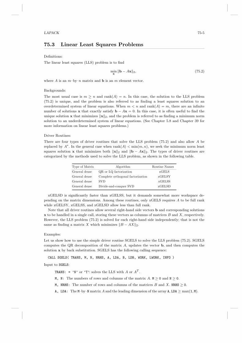
75.3 Linear Least Squares Problems
Definitions:
The linear least squares (LLS) problem is to find
minx
‖b − Ax‖2, (75.2)
where A is an m–by–n matrix and b is an m element vector.
Backgrounds:
The most usual case is m ≥ n and rank(A) = n. In this case, the solution to the LLS problem
(75.2) is unique, and the problem is also referred to as finding a least squares solution to an
overdetermined system of linear equations. When m < n and rank(A) = m, there are an infinite
number of solutions x that exactly satisfy b − Ax = 0. In this case, it is often useful to find the
unique solution x that minimizes ‖x‖2, and the problem is referred to as finding a minimum norm
solution to an underdetermined system of linear equations. (See Chapter 5.8 and Chapter 39 for
more information on linear least squares problems.)
Driver Routines:
There are four types of driver routines that solve the LLS problem (75.2) and also allow A be
replaced by A∗. In the general case when rank(A) < min(m, n), we seek the minimum norm least
squares solution x that minimizes both ‖x‖2 and ‖b − Ax‖2. The types of driver routines are
categorized by the methods used to solve the LLS problem, as shown in the following table.
Type of Matrix Algorithm Routine Names
General dense QR or LQ factorization xGELS
General dense Complete orthogonal factorization xGELSY
General dense SVD xGELSS
General dense Divide-and-conquer SVD xGELSD
xGELSD is significantly faster than xGELSS, but it demands somewhat more workspace de-
pending on the matrix dimensions. Among these routines, only xGELS requires A to be full rank
while xGELSY, xGELSS, and xGELSD allow less than full rank.
Note that all driver routines allow several right-hand side vectors b and corresponding solutions
x to be handled in a single call, storing these vectors as columns of matrices B and X, respectively.
However, the LLS problem (75.2) is solved for each right-hand side independently; that is not the
same as finding a matrix X which minimizes ‖B − AX‖2.
Examples:
Let us show how to use the simple driver routine SGELS to solve the LLS problem (75.2). SGELS
computes the QR decomposition of the matrix A, updates the vector b, and then computes the
solution x by back substitution. SGELS has the following calling sequence:
CALL SGELS( TRANS, M, N, NRHS, A, LDA, B, LDB, WORK, LWORK, INFO )
Input to SGELS:
TRANS: = ’N’ or ’T’: solves the LLS with A or AT .
M, N: The numbers of rows and columns of the matrix A. M ≥ 0 and N ≥ 0.
M, NRHS: The number of rows and columns of the matrices B and X. NRHS ≥ 0.
A, LDA: The M–by–N matrix A and the leading dimension of the array A, LDA ≥ max(1, M).

75-6 Handbook of Linear Algebra
B, LDB: The matrix B and the leading dimension of the array B, LDB ≥ max(1, M, N).
If TRANS = ’N’, then B is M–by–NRHS. If TRANS = ’T’, then B is N–by–NRHS.
WORK, LWORK: The workspace array and its dimension. LWORK ≥ min(M, N) + max(1, M, N, NRHS).
If LWORK = −1, then a workspace query is assumed; the routine only calculates
the optimal size of the WORK array, and returns this value as the first entry of
the WORK array.
Output from SGELS:
B: It is overwritten by the solution vectors, stored columnwise.
• If TRANS = ’N’ and M ≥ N, rows 1 to N of B contain the solution vectors of the
LLS problem minx ‖b − Ax‖2; the residual sum of squares in each column is
given by the sum of squares of elements N + 1 to M in that column;
• If TRANS = ’N’ and M < N, rows 1 to N of B contain the minimum norm solution
vectors of the underdetermined system AX = B;
• If TRANS = ’T’ and M ≥ N, rows 1 to M of B contain the minimum norm solution
vectors of the underdetermined system AT X = B;
• If TRANS = ’T’ and M < N, rows 1 to M of B contain the solution vectors of the
LLS problem minx ‖b−AT x‖2; the residual sum of squares for the solution in
each column is given by the sum of the squares of elements M+1 to N in that
column.
WORK: If INFO = 0, WORK(1) returns the optimal LWORK.
INFO: INFO = 0 if successful exit. If INFO = −j, the jth input argument had an illegal
value.
Consider an LLS problem (75.2) with a 6–by–5 matrix A and a 6–by–1 matrix b:
A =
2
6
6
6
6
6
6
6
4
−74 80 18 −11 −4
14 −69 21 28 0
66 −72 −5 7 1
−12 66 −30 −23 3
3 8 −7 −4 1
4 −12 4 4 0
3
7
7
7
7
7
7
7
5
and b =
2
6
6
6
6
6
6
6
4
51
−61
−56
69
10
−12
3
7
7
7
7
7
7
7
5
.
The exact solution of the LLS problem is x =h
1 2 −1 3 −4iT
with residual ‖b−Ax‖2 = 0.
Upon calling SGELS, the first 5 elements of B are overwritten by the solution vector x:
x =
2
6
6
6
6
6
4
1.0000176
2.0000196
−0.9999972
3.0000386
−4.0000405
3
7
7
7
7
7
5
,
while the sixth element of B contains the residual sum of squares 0.0000021. With M = 6, N = 5, NRHS = 1,
LWORK has been set to 11. For such a small matrix, the minimal workspace is also the optimal
workspace.

LAPACK 75-7
75.4 The Linear Equality-Constrained Least Squares Prob-
lem
Definitions:
The linear equality-constrained least squares (LSE) problem is
minx
‖c − Ax‖2 subject to Bx = d, (75.3)
where A is an m–by–n matrix and B is a p–by–n matrix, c is an m-vector, and d is a p-vector,
with p ≤ n ≤ m + p.
Backgrounds:
Under the assumptions that B has full row rank p and the matrix
"
A
B
#
has full column rank n, the
LSE problem (75.3) has a unique solution x.

75-8 Handbook of Linear Algebra
Driver Routines:
The driver routine for solving the LSE is xGGLSE, which uses a generalized QR factorization of
the matrices A and B.
Examples:
Let us show how to use the driver routine SGGLSE to solve the LSE problem (75.3). SGGLSE first
computes a generalized QR decomposition of A and B, and then computes the solution by back
substitution. SGGLSE has the following calling sequence:
CALL SGGLSE( M, N, P, A, LDA, B, LDB, C, D, X, WORK, LWORK, INFO )
Input to SGGLSE:
M, P: The numbers of rows of the matrices A and B, respectively. M ≥ 0 and P ≥0.
N: The number of columns of the matrices A and B. N ≥ 0. Note that 0 ≤ P ≤ N
≤ M+P.
A, LDA: The M–by–N matrix A and the leading dimension of the array A. LDA ≥max(1,M).
B, LDB: The P–by–N matrix B and the leading dimension of the array B. LDB ≥max(1,P).
C, D: The right-hand side vectors for the least squares part, and the constrained
equation part of the LSE, respectively.
WORK, LWORK: The workspace array and its dimension. LWORK ≥ max(1, M + N + P).
If LWORK = −1, then a workspace query is assumed; the routine only calculates
the optimal size of the WORK array, and returns this value as the first entry of
the WORK array.
Output from SGGLSE:
C: The residual sum of squares for the solution is given by the sum of squares of
elements N-P+1 to M of vector C.
X: The solution of the LSE problem.
WORK: If INFO = 0, WORK(1) returns the optimal LWORK.
INFO: = 0 if successful exit. If INFO = −j, the jth argument had an illegal value.
Let us demonstrate the use of SGGLSE to solve the LSE problem (75.3), where
A =
2
6
6
6
4
1 1 1
1 3 1
1 −1 1
1 1 1
3
7
7
7
5
, B =
"
1 1 1
1 1 −1
#
, c =
2
6
6
6
4
1
2
3
4
3
7
7
7
5
, d =
"
7
4
#
.
The unique exact solution is x = 18[46 −2 12]T . Upon calling SGGLSE with this input data and
M = 4, N = 3, P = 2, LWORK = 9, an approximate solution of the LSE problem is returned in X:
X = [5.7500000 −0.2500001 1.4999994]T .
The array C is overwritten by the residual sum of squares for the solution:
C = [4.2426405 8.9999981 2.1064947 0.2503501]T .

LAPACK 75-9
75.5 A General Linear Model Problem
Definitions:
The general linear model (GLM) problem is
minx,y
‖y‖2 subject to d = Ax + By, (75.4)
where A is an n–by–m matrix, B is an n–by–p matrix, and d is a n-vector, with m ≤ n ≤ m + p.
Backgrounds:
When B = I, the problem reduces to an ordinary linear least squares problem (75.2). When B
is square and nonsingular, the GLM problem is equivalent to the weighted linear least squares
problem:
minx
‖B−1(d − Ax)‖2.
Note that the GLM is equivalent to the LSE problem
minx,y
‚
‚
‚
‚
‚
0 −h
0 Ii
"
x
y
#‚
‚
‚
‚
‚
2
subject toh
A Bi
"
x
y
#
= d.
Therefore, the GLM problem has a unique solution of the matrix
"
0 I
A B
#
and has full column
rank m + p.
Driver Routines:
The driver routine for solving the GLM problem (75.4) is xGGGLM, which uses a generalized QR
factorization of the matrices A and B.
Examples:
Let us show how to use the driver routine SGGGLM to solve the GLM problem (75.4). SGGGLM
computes a generalized QR decomposition of the matrices A and B, and then computes the solution
by back substitution. SGGGLM has the following calling sequence:
CALL SGGGLM( N, M, P, A, LDA, B, LDB, D, X, Y, WORK, LWORK, INFO )
Input to SGGGLM:
N: The number of rows of the matrices A and B. N ≥ 0.
M, P: The number of columns of the matrices A and B, respectively. 0 ≤ M ≤ N
and P ≥ N-M.
A, LDA: The N–by–M matrix A and the leading dimension of the array A. LDA ≥max(1,N).
B, LDB: The N–by–P matrix B and the leading dimension of the array B. LDB ≥max(1,N).
D: The left-hand side of the GLM equation.
WORK, LWORK: The workspace array and its dimension. LWORK ≥ max(1,N+M+P).
If LWORK = -1, then a workspace query is assumed; the routine only calculates
the optimal size of the WORK array, and returns this value as the first entry of
the WORK array.
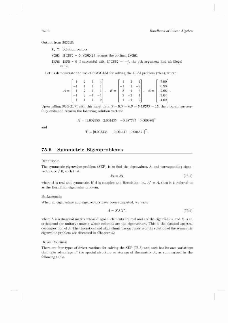
75-10 Handbook of Linear Algebra
Output from SGGGLM:
X, Y: Solution vectors.
WORK: If INFO = 0, WORK(1) returns the optimal LWORK.
INFO: INFO = 0 if successful exit. If INFO = −j, the jth argument had an illegal
value.
Let us demonstrate the use of SGGGLM for solving the GLM problem (75.4), where
A =
2
6
6
6
6
6
4
1 2 1 4
−1 1 1 1
−1 −2 −1 1
−1 2 −1 −1
1 1 1 2
3
7
7
7
7
7
5
, B =
2
6
6
6
6
6
4
1 2 2
−1 1 −2
3 1 6
2 −2 4
1 −1 2
3
7
7
7
7
7
5
, d =
2
6
6
6
6
6
4
7.99
0.98
−2.98
3.04
4.02
3
7
7
7
7
7
5
.
Upon calling SGGGLM with this input data, N = 5, M = 4, P = 3, LWORK = 12, the program success-
fully exits and returns the following solution vectors:
X = [1.002950 2.001435 −0.987797 0.009080]T
and
Y = [0.003435 −0.004417 0.006871]T .
75.6 Symmetric Eigenproblems
Definitions:
The symmetric eigenvalue problem (SEP) is to find the eigenvalues, λ, and corresponding eigen-
vectors, x 6= 0, such that
Ax = λx, (75.5)
where A is real and symmetric. If A is complex and Hermitian, i.e., A∗ = A, then it is referred to
as the Hermitian eigenvalue problem.
Backgrounds:
When all eigenvalues and eigenvectors have been computed, we write
A = XΛX∗, (75.6)
where Λ is a diagonal matrix whose diagonal elements are real and are the eigenvalues, and X is an
orthogonal (or unitary) matrix whose columns are the eigenvectors. This is the classical spectral
decomposition of A. The theoretical and algorithmic backgrounds is of the solution of the symmetric
eigenvalue problem are discussed in Chapter 42.
Driver Routines:
There are four types of driver routines for solving the SEP (75.5) and each has its own variations
that take advantage of the special structure or storage of the matrix A, as summarized in the
following table.

LAPACK 75-11
Types of Matrix Routine Names
(Storage Scheme) Simple Driver Divide-and-Conquer Expert Driver RRR Driver
General symmetric xSYEV xSYEVD xSYEVX xSYEVR
General symmetric
(packed storage) xSPEV xSPEVD xSPEVX –
Band matrix xSBEV xSBEVD xSBEVX –
Tridiagonal matrix xSTEV xSTEVD xSTEVX xSTEVR
The simple driver computes all eigenvalues and (optionally) eigenvectors. The expertdriver computes all or a selected subset of the eigenvalues and (optionally) eigenvectors.The divide-and-conquer driver has the same functionality as, yet outperforms, the simpledriver, but it requires more workspace. The relative robust representation (RRR) drivercomputes all or a subset of the eigenvalues and (optionally) the eigenvectors. The last oneis generally faster than any other types of driver routines and uses the least amount ofworkspace.
Examples:
Let us show how to use the simple driver SSYEV to solve the SEP (75.5) by computing the spectral
decomposition (75.6). SSYEV first reduces A to a tridiagonal form, and then uses the implicit QL
or QR algorithm to compute eigenvalues and optionally eigenvectors. SSYEV has the following
calling sequence:
CALL SSYEV( JOBZ, UPLO, N, A, LDA, W, WORK, LWORK, INFO )
Input to SSYEV:
JOBZ: = ’N’, compute eigenvalues only;
= ’V’, compute eigenvalues and eigenvectors.
UPLO: = ’U’, the upper triangle of A is stored in the array A; if UPLO = ’L’, the
lower triangle of A is stored.
N: The order of the matrix A. N ≥ 0.
A, LDA: The symmetric matrix A and the leading dimension of the array A. LDA ≥max(1,N).
WORK, LWORK: The workspace array and its dimension. LWORK ≥ max(1, 3 ∗ N− 1).
If LWORK = −1, then a workspace query is assumed; the routine only calculates
the optimal size of the WORK array, and returns this value as the first entry of
the WORK array.
Output from SSYEV:
A: The orthonormal eigenvectors X, if JOBZ = ’V’.
W: The eigenvalues λ in ascending order.
WORK: If INFO = 0, WORK(1) returns the optimal LWORK.
INFO: = 0 if successful exit. If INFO = −j, the jth input argument had an illegal
value. If INFO = j, the j off-diagonal elements of an intermediate tridiagonal
form did not converge to zero.
Let us demonstrate the use of SSYEV to solve the SEP (75.5), where
A =
2
6
6
6
4
5 4 1 1
4 5 1 1
1 1 4 2
1 1 2 4
3
7
7
7
5
.

75-12 Handbook of Linear Algebra
The exact eigenvalues are 1, 2, 5, and 10. Upon calling SSYEV with the matrix A and N = 4,
LWORK = 3 ∗ N− 1 = 11, A is overwritten by its orthonormal eigenvectors X.
X =
2
6
6
6
4
0.7071068 −0.0000003 0.3162279 0.6324555
−0.7071068 0.0000001 0.3162278 0.6324555
0.0000002 0.7071069 −0.6324553 0.3162278
−0.0000001 −0.7071066 −0.6324556 0.3162278
3
7
7
7
5
.
The eigenvalues that correspond to the eigenvectors in each column of X are returned in W:
W = [0.9999996 1.9999999 4.9999995 10.0000000].
75.7 Nonsymmetric Eigenproblems
As is customary in numerical linear algebra, in this section the term left eigenvector ofA means a (column) vector y such that y∗A = λy∗. This is contrary to the definition inSection 4.3, under which y∗ would be called a left eigenvector.
Definitions:
The nonsymmetric eigenvalue problem (NEP) is to find the eigenvalues, λ, and corresponding
(right) eigenvectors, x 6= 0, such thatAx = λx (75.7)
and, perhaps, the left eigenvectors, y 6= 0, satisfying
y∗A = λy
∗. (75.8)
Backgrounds:
The problem is solved by computing the Schur decomposition of A, defined in the real case as
A = ZTZT ,
where Z is an orthogonal matrix and T is an upper quasi-triangular matrix with 1–by–1 and 2–by–2
diagonal blocks, the 2–by–2 blocks corresponding to complex conjugate pairs of eigenvalues of A.
In the complex case, the Schur decomposition is
A = ZTZ∗,
where Z is unitary and T is a complex upper triangular matrix.
The columns of Z are called the Schur vectors. For each k (1 ≤ k ≤ n), the first k columns of
Z form an orthonormal basis for the invariant subspace corresponding to the first k eigenvalues
on the diagonal of T . It is possible to order the Schur factorization so that any desired set of k
eigenvalues occupies the k leading positions on the diagonal of T . The theoretical and algorithmic
background of the solution of the nonsymmetric eigenvalue problem is discussed in Chapter 43.
Driver Routines:
Both the simple driver xGEEV and expert driver xGEEVX are provided. The simple driver com-
putes all the eigenvalues of A and (optionally) the right or left eigenvectors (or both). The expert
driver performs the same task as the simple driver plus the additional feature that it balances the
matrix to try to improve the conditioning of the eigenvalues and eigenvectors, and it computes the
condition numbers for the eigenvalues or eigenvectors (or both).
Examples:
Let us show how to use the simple driver SGEEV to solve the NEP (75.7). SGEEV first reduces
A to an upper Hessenberg form (a Hessenberg matrix is a matrix where all entries below the
first lower subdiagonal are zeros), and then uses the implicit QR algorithm to compute the Schur
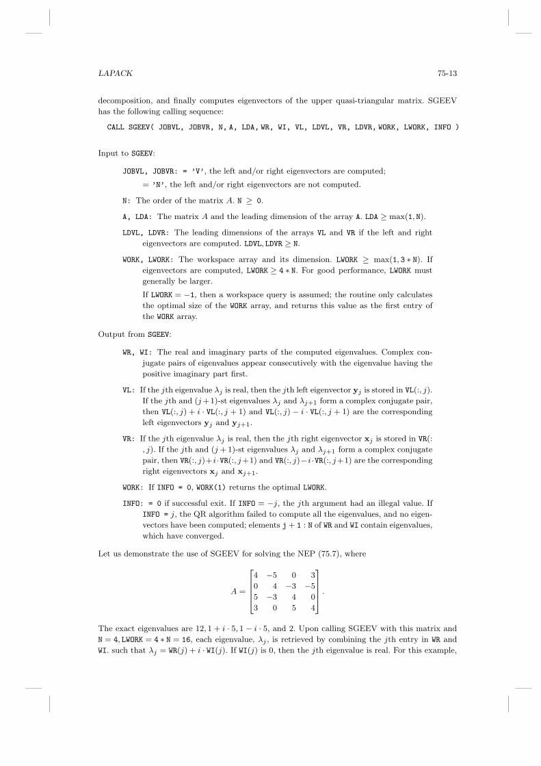
LAPACK 75-13
decomposition, and finally computes eigenvectors of the upper quasi-triangular matrix. SGEEV
has the following calling sequence:
CALL SGEEV( JOBVL, JOBVR, N, A, LDA, WR, WI, VL, LDVL, VR, LDVR, WORK, LWORK, INFO )
Input to SGEEV:
JOBVL, JOBVR: = ’V’, the left and/or right eigenvectors are computed;
= ’N’, the left and/or right eigenvectors are not computed.
N: The order of the matrix A. N ≥ 0.
A, LDA: The matrix A and the leading dimension of the array A. LDA ≥ max(1, N).
LDVL, LDVR: The leading dimensions of the arrays VL and VR if the left and right
eigenvectors are computed. LDVL, LDVR ≥ N.
WORK, LWORK: The workspace array and its dimension. LWORK ≥ max(1, 3 ∗ N). If
eigenvectors are computed, LWORK ≥ 4 ∗ N. For good performance, LWORK must
generally be larger.
If LWORK = −1, then a workspace query is assumed; the routine only calculates
the optimal size of the WORK array, and returns this value as the first entry of
the WORK array.
Output from SGEEV:
WR, WI: The real and imaginary parts of the computed eigenvalues. Complex con-
jugate pairs of eigenvalues appear consecutively with the eigenvalue having the
positive imaginary part first.
VL: If the jth eigenvalue λj is real, then the jth left eigenvector yj is stored in VL(:, j).
If the jth and (j +1)-st eigenvalues λj and λj+1 form a complex conjugate pair,
then VL(:, j) + i · VL(:, j + 1) and VL(:, j) − i · VL(:, j + 1) are the corresponding
left eigenvectors yj and yj+1.
VR: If the jth eigenvalue λj is real, then the jth right eigenvector xj is stored in VR(:
, j). If the jth and (j + 1)-st eigenvalues λj and λj+1 form a complex conjugate
pair, then VR(:, j)+i ·VR(:, j+1) and VR(:, j)−i ·VR(:, j+1) are the corresponding
right eigenvectors xj and xj+1.
WORK: If INFO = 0, WORK(1) returns the optimal LWORK.
INFO: = 0 if successful exit. If INFO = −j, the jth argument had an illegal value. If
INFO = j, the QR algorithm failed to compute all the eigenvalues, and no eigen-
vectors have been computed; elements j + 1 : N of WR and WI contain eigenvalues,
which have converged.
Let us demonstrate the use of SGEEV for solving the NEP (75.7), where
A =
2
6
6
6
4
4 −5 0 3
0 4 −3 −5
5 −3 4 0
3 0 5 4
3
7
7
7
5
.
The exact eigenvalues are 12, 1 + i · 5, 1 − i · 5, and 2. Upon calling SGEEV with this matrix and
N = 4, LWORK = 4 ∗ N = 16, each eigenvalue, λj , is retrieved by combining the jth entry in WR and
WI. such that λj = WR(j) + i · WI(j). If WI(j) is 0, then the jth eigenvalue is real. For this example,

75-14 Handbook of Linear Algebra
we have
λ1 = 12.0000000
λ2 = 1.000000 + i · 5.0000005
λ3 = 1.000000 − i · 5.0000005
λ4 = 1.9999999.
The left eigenvectors are stored in VL. Since the first and fourth eigenvalues are real, their eigenvec-
tors are the corresponding columns in VL, that is, y1 = VL(:, 1) and y4 = VL(:, 4). Since the second
and third eigenvalues form a complex conjugate pair, the second eigenvector, y2 = VL(:, 2)+i·VL(:, 3)
and the third eigenvector, y3 = VL(:, 2) − i · VL(:, 3). If we place all the eigenvectors in a matrix Y
where Y = [y1,y2,y3,y4], we have
Y =
2
6
6
6
4
−0.5000001 0.0000003 − i · 0.4999999 0.0000003 + i · 0.4999999 0.5000000
0.4999999 −0.5000002 −0.5000002 0.5000001
−0.5000000 −0.5000000 − i · 0.0000002 −0.5000000 + i · 0.0000002 −0.4999999
−0.5000001 −0.0000003 + i · 0.5000000 −0.0000003 − i · 0.5000000 0.5000001
3
7
7
7
5
.
The right eigenvectors xj can be recovered from VR in the way similar to the left eigenvectors. The
right eigenvector matrix X is
X =
2
6
6
6
4
−0.5000000 0.5000002 0.5000002 0.5000001
0.4999999 −0.0000001 − i · 0.5000000 −0.0000001 + i · 0.5000000 0.5000000
−0.5000000 −0.0000001 − i · 0.4999999 −0.0000001 + i · 0.4999999 −0.5000000
−0.5000001 −0.5000001 −0.5000001 0.5000000
3
7
7
7
5
.
75.8 Singular Value Decomposition
Definitions:
The singular value decomposition (SVD) of an m–by–n matrix A is
A = UΣV T (A = UΣV ∗ in the complex case), (75.9)
where U and V are orthogonal (unitary) and Σ is an m–by–n diagonal matrix with real diagonal
elements, σj , such that
σ1 ≥ σ2 ≥ . . . ≥ σmin(m, n) ≥ 0.
The σj are the singular values of A and the first min(m, n) columns of U and V are the left and
right singular vectors of A.
Backgrounds:
The singular values σj and the corresponding left singular vectors uj and right singular vectors vj
satisfy
Avj = σjuj and ATuj = σjvj (or A∗
uj = σjvj in complex case),
where uj and vj are the jth columns of U and V , respectively. (See Chapter 17 and Chapter 45
for more information on singular value decompositions.)

LAPACK 75-15
Driver Routines:
Two types of driver routines are provided in LAPACK. The simple driver xGESVD computes,
all the singular values and (optionally) left and/or right singular vectors. The divide and conquer
driver xGESDD has the same functionality as the simple driver except that it is much faster for
larger matrices, but uses more workspace.
Examples:
Let us show how to use the simple driver SGESVD to compute the SVD (75.9). SGESVD first
reduces A to a bidiagonal form, and then uses an implicit QR-type algorithm to compute singular
values and optionally singular vectors. SGESVD has the following calling sequence:
CALL SGESVD( JOBU, JOBVT, M, N, A, LDA, S, U, LDU, VT, LDVT, WORK,
LWORK, INFO )
Input to SGESVD:
JOBU: Specifies options for computing all or part of the left singular vectors U :
= ’A’, all M columns of U are returned in the array U:
= ’S’, the first min(M,N) columns of U are returned;
= ’O’, the first min(M,N) columns of U are overwritten on the array A;
= ’N’, no left singular vectors are computed. Note that JOBVT and JOBU cannot
both be ’O’.
JOBVT: Specifies options for computing all or part of the right singular vectors VT:
= ’A’, all N rows of V T are returned in the array VT;
= ’S’, the first min(M,N) rows of V T are returned;
= ’O’, the first min(M,N) rows of V T are overwritten on the array A;
= ’N’, no right singular vectors are computed.
M, N: The number of rows and columns of the matrix A. M, N ≥ 0.
A, LDA: The M–by–N matrix A and the leading dimension of the array A. LDA ≥max(1,M).
LDU, LDVT: The leading dimension of the arrays U and VT. LDU, LDVT ≥ 1;
If JOBU = ’S’ or ’A’, LDU ≥ M.
If JOBVT = ’A’, LDVT ≥ N; If JOBVT = ’S’, LDVT ≥min(M, N).
WORK, LWORK: The workspace array and its dimension. LWORK ≥ max(3 min(M, N) +
max(M, N), 5 min(M, N)).
If LWORK = -1, then a workspace query is assumed; the routine only calculates
the optimal size of the WORK array and returns this value as the first entry of the
WORK array.
Output from SGESVD:
A: If JOBU = ’O’, A is overwritten with the first min(M, N) columns of U (the left
singular vectors, stored columnwise);
If JOBVT = ’O’, A is overwritten with the first min(M,N) rows of V T (the right
singular vectors, stored rowwise);
S: Singular values of A, sorted so that S(i) ≥ S(i + 1).
U: If JOBU = ’A’, U contains M–by–M orthogonal matrix U . If JOBU = ’S’, U contains
the first min(M,N) columns of U . If JOBU = ’N’ or ’O’, U is not referenced.

75-16 Handbook of Linear Algebra
VT: If JOBVT = ’A’, VT contains right N–by–N orthogonal matrix V T . If JOBVT =
’S’, VT contains the first min(M,N) rows of VT (the right singular vectors stored
rowwise). If JOBVT = ’N’ or ’O’, VT is not referenced.
WORK: If INFO = 0, WORK(1) returns the optimal LWORK.
INFO: = 0 if successful exit. If INFO = −j, the jth argument had an illegal value. If
INFO > 0, the QR-type algorithm (subroutine SBDSQR) did not converge. INFO
specifies how many superdiagonals of an intermediate bidiagonal form B did
not converge to zero. WORK(2:min(M,N)) contains the unconverged superdiagonal
elements of an upper bidiagonal matrix B whose diagonal is in S (not necessarily
sorted). B satisfies A = UBV T , so it has the same singular values as A, and
singular vectors related by U and V T .
Let us show the numerical results of SGESVD in computing the SVD by an 8–by–5 matrix A as
follows:
A =
2
6
6
6
6
6
6
6
6
6
6
6
4
22 10 2 3 7
14 7 10 0 8
−1 13 −1 −11 3
−3 −2 13 −2 4
9 8 1 −2 4
9 1 −7 5 −1
2 −6 6 5 1
4 5 0 −2 2
3
7
7
7
7
7
7
7
7
7
7
7
5
.
The exact singular singular values are√
1248, 20,√
384, 0, 0. The rank of the matrix A is 3. Upon
calling SGESVD with M = 8, N = 5, LWORK = 25, the computed singular values of A are returned in
S:
S = [35.3270454 20.0000038 19.5959187 0.0000007 0.0000004].
The columns in U contain the left singular vectors U of A:
U =
2
6
6
6
6
6
6
4
-7.0711e-001 1.5812e − 001 −1.7678e − 001 2.4818e − 001 −4.0289e − 001 −3.2305e − 001 −3.3272e − 001 −6.9129e − 002
-5.3033e-001 1.5811e − 001 3.5355e − 001 −6.2416e − 001 2.5591e − 001 −3.9178e − 002 3.0548e − 001 −1.3725e − 001
-1.7678e-001 −7.9057e − 001 1.7677e − 001 3.0146e − 001 1.9636e − 001 −3.1852e − 001 2.3590e − 001 −1.6112e − 001
0 1.5811e − 001 7.0711e − 001 2.9410e − 001 3.1907e − 001 4.7643e − 002 −5.2856e − 001 7.1055e − 002
-3.5355e-001 −1.5811e − 001 −1.0000e − 006 2.3966e − 001 −7.8607e − 002 8.7800e − 001 1.0987e − 001 −5.8528e − 002
-1.7678e-001 1.5812e − 001 −5.3033e − 001 1.7018e − 001 7.9071e − 001 −7.0484e − 003 −9.0913e − 002 −8.3220e − 004
0 4.7434e − 001 1.7678e − 001 5.2915e − 001 −1.5210e − 002 −1.3789e − 001 6.6193e − 001 7.9763e − 002
-1.7678e-001 −1.5811e − 001 −1.0000e − 006 −7.1202e − 002 1.3965e − 002 −2.0712e − 002 4.9676e − 002 9.6726e − 001
3
7
7
7
7
7
7
5
.
The rows in VT contain the right singular vectors V T of A:
V T =
2
6
6
4
−8.0064e − 001 −4.8038e − 001 −1.6013e − 001 0 −3.2026e − 001
3.1623e − 001 −6.3246e − 001 3.1622e − 001 6.3246e − 001 −1.8000e − 006
−2.8867e − 001 −3.9000e − 006 8.6603e − 001 −2.8867e − 001 2.8868e − 001
−4.0970e − 001 3.4253e − 001 −1.2426e − 001 6.0951e − 001 5.7260e − 001
8.8224e − 002 −5.0190e − 001 −3.3003e − 001 −3.8100e − 001 6.9730e − 001
3
7
7
5
.
75.9 Generalized Symmetric Definite Eigenproblems
Definitions:
The generalized symmetric definite eigenvalue problem (GSEP) is to find the eigenvalues, λ, and
corresponding eigenvectors, x 6= 0, such that
Ax = λBx (type 1) (75.10)

LAPACK 75-17
orABx = λx (type 2) (75.11)
orBAx = λx (type 3) (75.12)
where A and B are symmetric or Hermitian and B is positive definite.
Backgrounds:
For all these problems the eigenvalues λ are real. The matrix Z of the computed eigenvectors
satisfies Z∗AZ = Λ (problem types 1 and 3) or Z−1AZ−∗ = I (problem type 2), where Λ is a
diagonal matrix with the eigenvalues on the diagonal. Z also satisfies Z∗BZ = I (problem types
1 and 2) or Z∗B−1Z = I (problem type 3). These results are consequences of spectral theory for
symmetric matrices. For example, the GSEP type 1 can be rearranged as
B− 1
2 AB− 1
2 y = λy,
where y = B1
2 x.
Driver Routines:
There are three types of driver routines for solving the GSEP, and each has variations that take
advantage of the special structure or storage of the matrices A and B, as shown in the following
table:
Types of Matrix Routine Names
(Storage Scheme) Simple Driver Divide-and-Conquer Expert Driver
General dense xSYGV/xHEGV xSYGVD/xHEGVD xSYGVX/xHEGVX
General dense
(packed storage) xSPGV/xHPGV xSPGVD/xHPGVD xSPGVX/xHPGVX
Band matrix xSBGV/xHBGV xSBBVD/xHBGVD xSBGVX/xHBGVX
The simple driver computes all the eigenvalues and (optionally) the eigenvectors. The expert
driver computes all or a selected subset of the eigenvalues and (optionally) eigenvectors. The divide-
and-conquer driver solves the same problem as the simple driver. It is much faster than the simple
driver, but uses more workspace.
Examples:
Let us show how to use the simple driver SSYGV to compute the GSEPs (75.10), (75.11), and
(75.12). SSGYV first reduces each of these problems to a standard symmetric eigenvalue problem,
using a Cholesky decomposition of B, and then computes eigenvalues and eigenvectors of the stan-
dard symmetric eigenvalue problem by an implicit QR-type algorithm. SSYGV has the following
calling sequence:
CALL SSYGV( ITYPE, JOBZ, UPLO, N, A, LDA, B, LDB, W, WORK, LWORK, INFO ) Input to SSYGV:
ITYPE: Specifies the problem type to be solved:
JOBZ: = ’N’, compute eigenvalues only;
= ’V’, compute eigenvalues and eigenvectors.
UPLO: = ’U’, the upper triangles of A and B are stored;
= ’L’, the lower triangles of A and B are stored.
N: The order of the matrices A and B. N ≥ 0.
A, LDA: The symmetric matrix A and the leading dimension of the array A. LDA ≥max(1,N).

75-18 Handbook of Linear Algebra
B: The symmetric positive definite matrix B and the leading dimension of the array
B. LDB ≥ max(1,N).
WORK, LWORK: The workspace array and its length. LWORK ≥ max(1, 3 ∗ N− 1).
If LWORK = −1, then a workspace query is assumed; the routine only calculates
the optimal size of the WORK array, and returns this value as the first entry of
the WORK array.
Output from SSYGV:
A: Contains the normalized eigenvector matrix Z if requested.
B: If INFO ≤ N, the part of B containing the matrix is overwritten by the triangular
factor U or L from the Cholesky factorization B = UT U or B = LLT .
W: The eigenvalues in ascending order.
WORK: If INFO = 0, WORK(1) returns the optimal LWORK.
INFO: = 0, then successful exit. If INFO = −j, then the jth argument had an illegal
value. If INFO > 0, then SSYGV returned an error code:
• INFO ≤ N: if INFO = j, the algorithm failed to converge;
• INFO > N: if INFO = N + j, for 1 ≤ j ≤ N, then the leading minor of order j
of B is not positive definite. The factorization of B could not be completed
and no eigenvalues or eigenvectors were computed.
Let us show the use of SSYGV to solve the type 1 GSEP (75.10) for the following 5–by–5 matrices
A and B:
A =
2
6
6
6
6
6
4
10 2 3 1 1
2 12 1 2 1
3 1 11 1 −1
1 2 1 9 1
1 1 −1 1 15
3
7
7
7
7
7
5
and B =
2
6
6
6
6
6
4
12 1 −1 2 1
1 14 1 −1 1
−1 1 16 −1 1
2 −1 −1 12 −1
1 1 1 −1 11
3
7
7
7
7
7
5
.
Upon calling SSYGV with N = 5, LWORK = 3 ∗ N− 1 = 14, A is overwritten by the eigenvector matrix
Z:
Z =
2
6
6
6
6
6
4
−0.1345906 0.0829197 −0.1917100 0.1420120 −0.0763867
0.0612948 0.1531484 0.1589912 0.1424200 0.0170980
0.1579026 −0.1186037 −0.0748390 0.1209976 −0.0666645
−0.1094658 −0.1828130 0.1374690 0.1255310 0.0860480
0.0414730 0.0035617 −0.0889779 0.0076922 0.2894334
3
7
7
7
7
7
5
.
The corresponding eigenvalues are returned in W:
W =h
0.4327872 0.6636626 0.9438588 1.1092844 1.4923532i
.
75.10 Generalized Nonsymmetric Eigenproblems
Definitions:
The generalized nonsymmetric eigenvalue problem (GNEP) is to find the eigenvalues, λ, and cor-
responding (right) eigenvectors, x 6= 0, such that
Ax = λBx (75.13)
and optionally, the corresponding left eigenvectors y 6= 0, such that
y∗A = λy
∗B, (75.14)

LAPACK 75-19
where A and B are n–by–n matrices. In this section the terms right eigenvector and left eigenvector
are used as just defined.
Backgrounds:
Sometimes an equivalent notation is used to refer to the GNEP of the pair (A, B). The GNEP can
be solved via the generalized Schur decomposition of the pair (A, B), defined in the real case as
A = QSZT , B = QTZT ,
where Q and Z are orthogonal matrices, T is upper triangular, and S is an upper quasi-triangular
matrix with 1-by-1 and 2-by-2 diagonal blocks, the 2-by-2 blocks corresponding to complex conju-
gate pairs of eigenvalues. In the complex case, the generalized Schur decomposition is
A = QSZ∗, B = QTZ∗,
where Q and Z are unitary and S and T are both upper triangular. The columns of Q and Z are
called left and right generalized Schur vectors and span pairs of deflating subspaces of A and B.
Deflating subspaces are a generalization of invariant subspaces: For each k, 1 ≤ k ≤ n, the first
k columns of Z span a right deflating subspace mapped by both A and B into a left deflating
subspace spanned by the first k columns of Q. It is possible to order the generalized Schur form so
that any desired subset of k eigenvalues occupies the k leading position on the diagonal of (S, T ).
(See Chapter 43 and Chapter 15 for more information on generalized eigenvalue problems.)
Driver Routines:
Both the simple and expert drivers are provided in LAPACK. The simple driver xGGEV computes
all eigenvalues of the pair (A, B), and optionally the left and/or right eigenvectors. The expert
driver xGGEVX performs the same task as the simple driver routines; in addition, it also balances
the matrix pair to try to improve the conditioning of the eigenvalues and eigenvectors, and computes
the condition numbers for the eigenvalues and/or left and right eigenvectors.
Examples:
Let us show how to use the simple driver SGGEV to solve the GNEPs (75.13) and (75.14). SGGEV
first reduces the pair (A, B) to generalized upper Hessenberg form (H, R), where H is upper Hes-
senberg (zero below the first lower subdiagonal) and R is upper triangular. Then SGGEV computes
the generalized Schur form (S, T ) of the generalized upper Hessenberg form (H, R), using an QZ
algorithm. The eigenvalues are computed from the diagonals of (S, T ). Finally, SGGEV computes
left and/or right eigenvectors if requested. SGGEV has the following calling sequence:
CALL SGGEV( JOBVL, JOBVR, N, A, LDA, B, LDB, ALPHAR, ALPHAI, BETA, VL, LDVL, VR, LDVR,
WORK, LWORK, INFO )
Input to SGGEV:
JOBVL, JOBVR: = ’N’, do not compute the left and/or right eigenvectors;
= ’V’, compute the left and/or right eigenvectors.
N: The order of the matrices A and B. N ≥ 0.
A, LDA: The matrix A and the leading dimension of the array A. LDA ≥ max(1,N).
B, LDB: The matrix B and the leading dimension of the array B. LDB ≥ max(1,N).
LDVL, LDVR: The leading dimensions of the eigenvector matrices VL and VR. LDVL, LDVR ≥ 1.
If eigenvectors are required, then LDVL, LDVR ≥ N.

75-20 Handbook of Linear Algebra
WORK, LWORK: The workspace array and its length. LWORK ≥ max(1, 8 ∗ N). For good
performance, LWORK must generally be larger.
If LWORK = −1, then a workspace query is assumed; the routine only calculates
the optimal size of WORK, and returns this value in WORK(1) on return.
Output from SGGEV:
ALPHAR, ALPHAI, BETA: (ALPHAR(j) + i · ALPHAI(j))/BETA(j) for j = 1, 2, . . . , N, are
the generalized eigenvalues. If ALPHAI(j) is zero, then the jth eigenvalue is real;
if positive, then the jth and (j +1)-st eigenvalues are a complex conjugate pair,
with ALPHAI(j + 1) negative.
VL: If JOBVL = ’V’, the left eigenvectors yj are stored in the columns of VL, in the
same order as their corresponding eigenvalues. If the jth eigenvalue is real, then
yj = VL(:, j), the jth column of VL. If the jth and (j + 1)th eigenvalues form
a complex conjugate pair, then yj = VL(:, j) + i · VL(:, j + 1) and yj+1 = VL(:
, j) − i · VL(:, j + 1).
VR: If JOBVR = ’V’, the right eigenvectors xj are stored one after another in the
columns of VR, in the same order as their eigenvalues. If the jth eigenvalue is
real, then xj = VR(:, j), the jth column of VR. If the jth and (j+1)th eigenvalues
form a complex conjugate pair, then xj = VR(:, j) + i · VR(:, j + 1) and xj+1 =
VR(:, j) − i · VR(:, j + 1).
WORK: If INFO = 0, WORK(1) returns the optimal LWORK.
INFO: INFO = 0 if successful exit. If INFO = −j, the jth argument had an illegal
value. If INFO = 1,...,N, then the QZ iteration failed. No eigenvectors have
been calculated, but ALPHAR(j), ALPHAI(j), and BETA(j) should be correct for j =
INFO + 1, . . . , N. If INFO = N+1, then other than QZ iteration failed in SHGEQZ.
If INFO = N+2, then error return from STGEVC.
Note that the quotients ALPHAR(j)/BETA(j) and ALPHAI(j)/BETA(j) may easily over- or underflow,
and BETA(j) may even be zero. Thus, the user should avoid naively computing the ratio. However,
ALPHAR and ALPHAI will be always less than and usually comparable to ‖A‖ in magnitude, and BETA
always less than and usually comparable to ‖B‖.Let us demonstrate the use of SGGEV in solving the GNEP of the following 6–by–6 matrices A
and B:
A =
2
6
6
6
6
6
6
6
4
50 −60 50 −27 6 6
38 −28 27 −17 5 5
27 −17 27 −17 5 5
27 −28 38 −17 5 5
27 −28 27 −17 16 5
27 −28 27 −17 5 16
3
7
7
7
7
7
7
7
5
and B =
2
6
6
6
6
6
6
6
4
16 5 5 5 −6 5
5 16 5 5 −6 5
5 5 16 5 −6 5
5 5 5 16 −6 5
5 5 5 5 −6 16
6 6 6 6 −5 6
3
7
7
7
7
7
7
7
5
.
The exact eigenvalues are 12
+ i ·√
32
, 12
+ i ·√
32
, 12− i ·
√3
2, 1
2− i ·
√3
2, ∞, ∞. Upon calling SGGEV
with N = 6, LWORK = 48, on exit, arrays ALPHAR, ALPHAI, and BETA are
ALPHAR =h
−25.7687130 6.5193458 5.8156629 5.8464251 5.5058141 11.2021322i
,
ALPHAI =h
0.0000000 11.2832556 −10.0653677 10.1340599 −9.5436525 0.0000000i
,
BETA =h
0.0000000 13.0169611 11.6119413 11.7124090 11.0300474 0.0000000i
.

LAPACK 75-21
Therefore, there are two infinite eigenvalues corresponding to BETA(1) = BETA(6) = 0 and four
finite eigenvalues λj = (ALPHAR(j) + i · ALPHAI(j))/BETA(j) for j = 2, 3, 4, 5.
(ALPHAR(2 : 5) + i · ALPHAI(2 : 5))/BETA(2 : 5) =
2
6
6
6
4
0.50083 + i · 0.86681
0.50083 − i · 0.86681
0.49917 + i · 0.86524
0.49917 − i · 0.86524
3
7
7
7
5
.
The left eigenvectors yj are stored in VL. Since ALPHAI(1) = ALPHAI(6) = 0, y1 = VL(:, 1) and y6 =
VL(:, 6). The second and third eigenvalues form a complex conjugate pair, the y2 = VL(:, 2)+i·VL(:, 3)
and y3 = VL(:, 2) − i · VL(:, 3). Similarly, y4 = VL(:, 4) + i · VL(:, 5) and y5 = VL(:, 4) + i · VL(:, 5). If
we place all the left eigenvectors in a matrix Y , where Y = [y1,y2,y3,y4,y5,y6], we have
Y =
2
6
6
6
4
−0.1666666 0.2632965 + i · 0.3214956 0.2632965 − i · 0.3214956 −0.4613968 + i · 0.1902102 −0.4613968 − i · 0.1902102 0.1666667
−0.1666666 −0.2834885 − i · 0.7165115 −0.2834885 + i · 0.7165115 0.9231794 − i · 0.0765849 0.9231794 + i · 0.0765849 0.1666667
−0.1666666 0.1623165 + i · 0.7526108 0.1623165 − i · 0.7526108 −0.9240005 − i · 0.0759995 −0.9240005 + i · 0.0759995 0.1666667
−0.1666666 0.0396326 − i · 0.4130635 0.0396326 + i · 0.4130635 0.4619284 + i · 0.1907958 0.4619284 − i · 0.1907958 0.1666666
−0.1666671 −0.0605860 + i · 0.0184893 −0.0605860 − i · 0.0184893 0.0000969 − i · 0.0761408 0.0000969 + i · 0.0761408 0.1666666
1.0000000 −0.0605855 + i · 0.0184900 −0.0605855 − i · 0.0184900 0.0000959 − i · 0.0761405 0.0000959 + i · 0.0761405 −1.0000000
3
7
7
7
5
.
The right eigenvectors can be recovered from VR in a way similar to the left eigenvectors. If we
place all the right eigenvectors in a matrix X, where X = [x1,x2,x3,x4,x5,x6], we have
U =
2
6
6
6
4
0.1666672 −0.2039835 − i · 0.5848466 −0.2039835 + i · 0.5848466 0.5722237 − i · 0.0237538 0.5722237 + i · 0.0237538 0.1666672
0.1666664 −0.7090308 − i · 0.2908980 −0.7090308 + i · 0.2908980 0.4485306 − i · 0.5514694 0.4485306 + i · 0.5514694 0.1666664
0.1666666 −0.7071815 + i · 0.2928185 −0.7071815 − i · 0.2928185 −0.0709520 − i · 0.7082051 −0.0709520 + i · 0.7082051 0.1666666
0.1666666 −0.2013957 + i · 0.5829236 −0.2013957 − i · 0.5829236 −0.4667411 − i · 0.3361499 −0.4667411 + i · 0.3361499 0.1666666
1.0000000 −0.2023994 + i · 0.0000001 −0.2023994 − i · 0.0000001 0.0536732 − i · 0.1799536 0.0536732 + i · 0.1799536 1.0000000
0.1666666 −0.2023991 − i · 0.0000002 −0.2023991 + i · 0.0000002 0.0536734 − i · 0.1799532 0.0536734 + i · 0.1799532 0.1666664
3
7
7
7
5
.
75.11 Generalized Singular Value Decomposition
Definitions:
The generalized (or quotient) singular value decomposition (GSVD or QSVD) of an m–by–n matrix
A and a p–by–n matrix B is given by the pair of factorizations
A = UΣ1
h
0 Ri
QT and B = V Σ2
h
0 Ri
QT . (75.15)
The matrices in these factorizations have the following properties:
• U is m–by–m, V is p–by–p, Q is n–by–n, and all three matrices are orthogonal. If A and B
are complex, these matrices are unitary instead of orthogonal, and QT should be replaced
by Q∗ in the pair of factorizations.
• R is r–by–r, upper triangular and nonsingular.h
0 Ri
is r–by–n (in other words, the 0 is
an r–by–(n − r) zero matrix). The integer r is the rank of
"
A
B
#
.
• Σ1 is m–by–r and Σ2 is p–by–r. Both are real, nonnegative, and diagonal, satisfying ΣT1 Σ1+
ΣT2 Σ2 = I. Write ΣT
1 Σ1 = diag(α21, . . . , α2
r) and ΣT2 Σ2 = diag(β2
1 , . . . , β2r ). The ratios αj/βj
for j = 1, 2, . . . , r are called the generalized singular values.
Σ1 and Σ2 have the following detailed structures, depending on whether m − r ≥ 0 or m − r < 0.
• In the first case, when m − r ≥ 0,
Σ1 =
0
B
@
k ℓ
k I 0
ℓ 0 C
m − k − ℓ 0 0
1
C
Aand Σ2 =
k ℓ
ℓ 0 S
p − ℓ 0 0
!
. (75.16)

75-22 Handbook of Linear Algebra
Here k+ℓ = r, and ℓ is the rank of B. C and S are diagonal matrices satisfying C2 +S2 = I,
and S is nonsingular. Let cj and sj be the diagonal entries of C and S, respectively. Then
we have α1 = · · · = αk = 1, αk+j = cj for j = 1, . . . , ℓ, β1 = · · · = βk = 0, and βk+j = sj
for j = 1, . . . , ℓ. Thus, the first k generalized singular values α1/β1, . . . , αk/βk are infinite
and the remaining ℓ generalized singular values are finite.
• In the second case, when m − r < 0,
Σ1 =
k m − k k + ℓ − m
k I 0 0
m − k 0 C 0
!
and Σ2 =
0
B
@
k m − k k + ℓ − m
m − k 0 S 0
k + ℓ − m 0 0 I
p − ℓ 0 0 0
1
C
A.
(75.17)
Again, k+ℓ = r, and ℓ is the rank of B. C and S are diagonal matrices satisfying C2+S2 = I,
and S is nonsingular. Let cj and sj be the diagonal entries of C and S, respectively. Then
we have α1 = · · · = αk = 1, αk+j = cj for j = 1, . . . , m − k, αm+1 = · · · = αr = 0, and
β1 = · · · = βk = 0, βk+j = sj for j = 1, . . . , m − k, βm+1 = · · · = βr = 1. Thus, the first
k generalized singular values α1/β1, . . . , αk/βk are infinite, and the remaining ℓ generalized
singular values are finite.
Backgrounds:
Here are some important special cases of the QSVD. First, when B is square and nonsingular, then
r = n and the QSVD of A and B is equivalent to the SVD of AB−1, where the singular values of
AB−1 are equal to the generalized singular values of A and B:
AB−1 = (UΣ1RQT )(V Σ2RQT )−1 = U(Σ1Σ−12 )V T .
Second, if the columns ofh
AT BTiT
are orthonormal, then r = n, R = I, and the QSVD of A
and B is equivalent to the CS (Cosine-Sine) decomposition ofh
AT BTiT
:
"
A
B
#
=
"
U 0
0 V
#"
Σ1
Σ2
#
QT .
Third, the generalized eigenvalues and eigenvectors of the pencil AT A − λBT B can be expressed
in terms of the QSVD of A and B, namely,
XT AT AX =
"
0 0
0 ΣT1 Σ1
#
and XT BT BX =
"
0 0
0 ΣT2 Σ2
#
,
where X = Q
"
I 0
0 R−1
#
. Therefore, the columns of X are the eigenvectors of AT A−λBT B, and the
“nontrivial” eigenvalues are the squares of the generalized singular values. “Trivial” eigenvalues are
those corresponding to the leading n− r columns of X, which span the common null space of AT A
and BT B.
The “trivial eigenvalues” are not well defined.1 (See Chapter 15 for more information on gen-
eralized singular value problems.)
1If we tried to compute the trivial eigenvalues in the same way as the nontrivial ones, that is by taking
ratios of the leading n − r diagonal entries of XT AT AX and XT BT BX, we would get 0/0.

LAPACK 75-23
Driver Routines:
The driver routine xGGSVD computes the GSVD (75.15) of A and B.
Examples:
Let us show how to use the driver routine SGGSVD to compute the QSVD (75.15). SGGSVD first
reduces the matrices A and B to a pair of triangular matrices, and then use a Jacobi-like method
to compute the QSVD of the triangular pair. SGGSVD has the following calling sequence:
CALL SGGSVD( JOBU, JOBV, JOBQ, M, N, P, K, L, A, LDA, B, LDB, ALPHA, BETA, U, LDU,
V, LDV, Q, LDQ, WORK, IWORK, INFO )
Input to SGGSVD:
JOBU, JOBV, JOBQ: , = ’U’, orthogonal matrices U , V and Q are computed;
= ’N’, these orthogonal matrices are not computed.
M, N, P: The number of rows or columns of the matrices A and B as defined in (15)
A, LDA: The M–by–N matrix A and the leading dimension of the array A. LDA ≥max(1, M).
B, LDB: The P–by–N matrix B and the leading dimension of the array B. LDB ≥max(1, P).
LDU, LDV, LDQ: The leading dimension of the arrays U, V, and Q if the orthogonal
matrices U , V , and Q are computed, LDU ≥ max(1, M), LDV ≥ max(1, P), LDQ ≥max(1, N).
WORK: The real workspace array, dimension max(3N, M, P) + N.
IWORK: The integer workspace array, dimension N.
Output from SGGSVD:
K, L: The dimension of the subblocks described in the definition of GSVD. K + L is
the effective numerical rank of the matrixh
AT BTiT
.
A: The entire triangular matrix R is stored in A(1:K+L,N-K-L+1:N) if m − r ≥ 0.
Otherwise, the subblock R(1 : m, 1 : k+ℓ) of R are stored in A(1:M,N-K-L+1:N).
B: The subblock R(m+1 : k+ℓ, m+1 : k+ℓ) of R are stored in B(M-K+1:L,N+M-K-L+1:N)
if m − r < 0.
ALPHA, BETA: The generalized singular value pairs;
ALPHA(1:K) = 1 and BETA(1:K) = 0.
• If M-K-L ≥ 0, then ALPHA(K + 1 : K + L) = C and BETA(K + 1 : K + L) = S.
• If M-K-L < 0, then
ALPHA(K + 1 : M) = C and ALPHA(M + 1 : K + L) = 0,
BETA(K + 1 : M) = S and BETA(M + 1 : K + L) = 1;
And ALPHA(K+L+1:N) = 0, BETA(K+L+1:N) = 0.
U, V, Q: Contains computed orthogonal matrices U , V , and Q if requested.
INFO: INFO = 0 if successful exit. If INFO = −j, then the jth argument had an illegal
value. If INFO = 1, the Jacobi-type procedure failed to converge.
Let us demonstrate the use of SGGSVD in computing the QSVD of the following 6–by–5 matrices
A

75-24 Handbook of Linear Algebra
and B:
A =
2
6
6
6
6
6
6
6
4
1 2 3 1 5
0 3 2 0 2
1 0 2 1 0
0 2 3 0 −1
1 0 2 1 1
0 2 1 0 1
3
7
7
7
7
7
7
7
5
and B =
2
6
6
6
6
6
6
6
4
1 −2 2 1 1
0 3 0 0 0
1 −2 2 1 1
0 2 0 0 0
2 −4 4 2 2
1 3 2 1 1
3
7
7
7
7
7
7
7
5
.
Upon calling SGGSVD with M = 6, P = 6, N = 5, LWORK = 20, we have K = 2 and L = 2. The QSVD
(75.15) of A and B falls in the first case (75.16) since M − K − L = 6 − 2 − 2 = 2 > 0. The arrays
ALPHA and BETA are
ALPHA =h
1.0000000 1.0000000 0.1537885 0.5788464 0.0000000i
,
BETA =h
0.0000000 0.0000000 0.9881038 0.8154366 0.0000000i
.
Hence, Σ1 and Σ2 have the structure as described in (75.16), namely,
Σ1 =
2
6
6
6
6
6
6
6
4
1 0 0 0
0 1 0 0
0 0 0.1537885 0
0 0 0 0.5788464
0 0 0 0
0 0 0 0
3
7
7
7
7
7
7
7
5
and Σ2 =
2
6
6
6
6
6
6
6
4
0 0 0.9881038 0
0 0 0 0.8154366
0 0 0 0
0 0 0 0
0 0 0 0
0 0 0 0
3
7
7
7
7
7
7
7
5
.
The first two generalized singular values are infinite, α1/β1 = α2/β2 = ∞, and the remaining two
generalized singular values are finite, α3/β3 = 0.15564 and α4/β4 = 0.70986.
Furthermore, the array A(1:4,2:5) contains the 4–by–4 upper triangular matrix R as defined
in (75.15):
R =
2
6
6
6
4
3.6016991 −1.7135643 −0.2843603 1.8104467
0 −2.6087811 −4.2943931 5.1107349
0 0 6.9692163 3.5063875
0 0 0 7.3144341
3
7
7
7
5
.
The orthogonal matrices U , V , and Q are returned in the arrays U, V, and Q, respectively:
U =
2
6
6
6
6
6
6
4
−0.6770154 −0.4872811 −0.4034495 −0.2450049 −0.2151961 0.1873468
−0.0947438 −0.5723576 0.4163284 0.1218751 0.0785425 −0.6848933
0.2098812 0.0670342 0.2612190 −0.7393155 −0.5670457 −0.1228532
0.6974092 −0.5903998 −0.3678919 0.0010751 −0.0196356 0.1712235
0.0000000 0.0000001 −0.0735656 −0.6152450 0.7822418 −0.0644937
−0.0473719 −0.2861788 0.6744684 −0.0019711 0.1170180 0.6687696
3
7
7
7
7
7
7
5
,
V =
2
6
6
6
6
6
6
4
−0.3017521 −0.2581125 0.9018297 −0.0002676 −0.1695592 −0.0166328
0.4354534 −0.2679386 0.1028928 0.0704557 0.2595005 −0.8097517
−0.3017520 −0.2581124 −0.1784097 −0.8828155 −0.0002829 −0.1764375
0.2903022 −0.1786257 −0.1298870 −0.0008522 −0.9259184 −0.0980879
−0.6035041 −0.5162248 −0.3568195 0.4625078 −0.0224125 −0.1660080
0.4240036 −0.7046767 −0.0097810 −0.0419325 0.2146671 0.5250862
3
7
7
7
7
7
7
5
,
Q =
2
6
6
6
6
4
−0.7071068 −0.2073452 −0.5604916 −0.0112638 −0.3777966
0.0000000 0.0000000 0.0000000 0.9995558 −0.0298012
0.0000001 0.5853096 0.2932303 −0.0225276 −0.7555932
0.7071067 −0.2073452 −0.5604916 −0.0112638 −0.3777965
−0.0000001 −0.7559289 0.5345224 −0.0112638 −0.3777965
3
7
7
7
7
5
.
References
[CLA] http://www.netlib.org/clapack/.
[JLA] http://www.netlib.org/java/f2j/.
[LUG99] E. Anderson, Z. Bai, C. Bischof, S. Blackford, J. Demmel, J. Dongarra, J. Du Croz,
A. Greenbaum, S. Hammarling, A. McKenney, and D. Sorensen, LAPACK Users’ Guide,
3rd ed., SIAM, Philadelphia, 1999.

LAPACK 75-25
[LAP] http://www.netlib.org/lapack/.
[LAP95] http://www.netlib.org/lapack95/.
[LA+] http://www.netlib.org/lapack++/.
[Sca] http://www.netlib.org/scalapack/.