Language and Wage Determination in a SegmentedUrban Labor Market

Qiang Li∗

Sauder School of BusinessUniversity of British Columbia

First Draft: December 2006This Draft: October 2008

Abstract

This paper presents a simple model of labor market segmentation. People ofdifferent language origins form separate urban labor submarkets. Using the 2001Census of Canada Public Use Microdata File on Individuals, I test the two keyimplications of the model. First, I find that English speaking workers earn morethan non-English speaking workers even though they all speak English at work.In addition, minority workers who do not speak English at home earn differentlydepending on which language they speak at the workplace. Second, wages in themajority labor market increase with the majority population. On the other hand,wages in the minority labor market decrease with the majority population, butthey increase with the minority population.

JEL Classification: J15, R23Keywords: Language, Labor Market Segmentation, Matching

1 Introduction

And the whole earth was of one language, and of one speech. ... Andthe Lord came down to see the city and the tower, which the children of menbuilded. And the Lord said, ‘Behold, the people is one, and they have all onelanguage; and this they begin to do: and now nothing will be restrained fromthem, which they have imagined to do.’(Genesis 11:1-6)

∗I thank Bob Helsley for the illuminating discussions that lead to this paper and his guidancethroughout this project. I am also grateful for suggestions by Tsur Somerville and David Green thatgreatly improve the structure and contents of this paper. Comments from Jim Brander, Keith Head,Sanghoon Lee and Hua Sun are also appreciated. All errors are my own.

1

Majority Labor Market ⇒

Minority Labor Market ⇒

Within-Labor-Market Wage Gap︷ ︸︸ ︷

Majority Workers Minority Workers

Majority Workers Minority Workers

Within-Language-GroupWage Gap

Figure 1: Illustration of the Language Theory of Labor Market Segmentation

Language is an important part of our lives. Our common knowledge about the words

and rules of a language facilitates our daily communications. In this paper, I study

whether language affects workers’ labor market outcomes and more importantly how it

exerts its influence. I present a labor market segmentation theory in which language

plays a central role. Figure 1 shows an illustration of this theory.

Workers in a city differ in two important respects. They belong to either the ma-

jority language group, which has a larger population, or the minority language group.

They also choose to enter either the majority labor market or the minority labor mar-

ket. The language groups are differentiated by individuals’ home languages, while the

labor market segments are distinguished by the languages commonly used in business

communications.1

Two types of wage gaps exist. As Figure 1 shows, the first type exists between

majority workers and minority workers who work in the majority labor market. This

gap is defined as Within-labor-market Wage Gap. In the majority market, a minority

worker can communicate in the majority language, but some tacit language barriers

hinder her ability to communicate effectively with her coworkers and manager.2 As a

result, she is not as productive as a majority worker, so she earns less.

The second type of wage gap exists between minority workers who work in different

1Notice in Figure 1 ‘majority workers in the minority market’ has been crossed to indicate that thoseworkers may not exist in reality. See the discussion in the model for details.

2See Lang (1986) or Wardhaugh (2005) for a discussion of the tacit nature of language.

2

labor market segments. I define this as Within-language-group Wage Gap. In the model,

a worker’s wage depends on the quality of the match between her job and her skill. The

majority labor market has a larger number of workers and firms, which means it can

offer a higher matching quality and a higher wage for workers. This market thickness

effect has been modeled by Helsley and Strange (1990).

Due to this market thickness effect, wages are correlated with language group pop-

ulations. First, the wages in the majority labor market are increasing as the majority

population increases. However, the wages in the minority labor market are decreasing as

the majority population increases. The former is a direct result of the market thickness

effect. The latter is because more minority workers will enter the majority labor market

as the wages in the majority labor market increase. The minority labor market retains

less workers, and hence offers lower wages.

Second, the wages in the minority labor market are increasing in the minority pop-

ulation due to the market thickness effect. However, the wages in the majority labor

market can either increase or decrease when the minority population increases. The lat-

ter is because the majority labor market can have either more or less minority workers

if the minority population increases. On the one hand, the additional minority workers

may enter the majority labor market. On the other hand, higher wages in the minority

labor market may attract minority workers who previously work in the majority labor

market to the minority market.

I tested the above implications of the model using the 2001 Canadian Census Public

Use Microdata on Individuals. One special feature of the data is the reported work

language. This feature allows me to identify a worker’s labor market segment by her

work language. Her language group can then be identified by her home language.

I find that workers who speak English (or French in Quebec) both at work and at

home get higher wages than those who speak English (or French in Quebec) at work

but speak minority languages at home. However, this gap is significantly reduced after I

3

control workers’ immigration ages, and occupation fixed effects. In addition, the return

to education and the return to work experience are higher for the former group of

workers. The second result is robust against including workers’ immigration ages and

occupations.

On the other hand, minority workers who speak English (or French in Quebec) at

work earn higher wages than those who speak their home languages at work. Moreover,

the return to education and the return to work experience are higher for the former.

Both results are robust against including workers’ immigration ages and occupations.

Next, I tested wages’ comparative statics with respect to population measures. How-

ever, both minority and majority populations may be endogenous. For example, a pos-

itive wage shock in a city may attract even more workers to this city, resulting in a

positive correlation between language group populations and the error term of a wage

equation.

To solve this problem, I constructed instrumental variables for both the minority

population and majority population.3 I employed Two Stage Least Squares (2SLS) to

test the predicted effects of population measures on workers’ wages. The signs of changes

predicted by the theory were confirmed. This pattern of comparative statics is unique

to the language theory of labor market segmentation, and hence it differentiates the

theory from the human capital view of language skills held by, for example, Chiswick

and Miller (1992, 1995) and Bleakley and Chin (2004), to name just a few.

This paper also differs from the seminal work of Lang (1986), who also explores

the relationship between language and wage determination. However, his economic

mechanism is quite different. In his model, it is the different capital to labor ratios of

different language groups that drive the wage gap. In this paper, the basic driving force

is the market thickness effect.

My model is also different from the traditional labor market segmentation litera-

3For details about these instruments section 4.1.4 and Appendix C.

4

ture(see Dickens and Lang, 1992, for a review of this literature). Most empirical research,

such as Dickens and Katz (1987) and Dickens and Lang (1985), focus on inter-industry

or inter-employer comparisons of wages. Language plays no role in these papers.

Various immigration policies can be analyzed within the framework of the model.

For example, the policy to encourage new immigrants to relocate into small cities is

likely to fail, especially for those who have lower language skills. They are much better

off to stay in big cities. The model, by relating immigration policies to changes in the

underlying model parameters, may be a useful tool for policy makers.

This paper consists of three parts. In the following section, a simple model with

two language groups and two labor markets is presented. Section 3 describes the major

source of data - the 2001 Canadian Census Public Use Microdata on Individuals. After

that, Section 4 presents my empirical results about wage gaps and the comparative

statics. Our results are then checked for their robustness. Finally, Section 5 concludes

with a discussion of the contributions of this paper and the direction of future work.

2 Model

2.1 Workers

In a city, workers belong to two language groups (indexed by superscript k). One is the

majority that has a larger population. The other has a smaller population and, hence,

is the minority group.4 The total number of workers of a language group is fixed. I

denote it by nk, where k ∈ d,m.The labor market in each city is segmented into two submarkets (indexed by subscript

l) in which the communication methods are different. In one labor market segment, the

common language of business is the majority group’s language. In the other labor

market, the common language of business is the minority language. The number of

4The majority language in the country may not always correspond to the majority language ofa particular city. One example would be the French in Quebec. While French people make up themajority in Quebec, French is not the majority language group in Canada.

5

workers in labor market l that come from language group k is denoted nkl , where k ∈

d,m and l ∈ ld, lm.There is no unemployment. Each worker has to sell one unit of labor. She works in

only one firm. She is perfectly mobile across the two labor submarkets. The problem for

her is to choose the labor submarket that maximizes her net wage. She is risk-neutral.

The uncertain net wage of a worker (indexed by second subscript i) is

Ukl,i = W k

l,i − θkl,i, (1)

where W kl,i is the uncertain wage of worker i who belongs to language group k and

works in labor submarket l, and θkl,i is the cost to learn a second language. The wage is

uncertain because the worker does not know how well her skills and experience will be

matched with her job, i.e., how high the matching quality will be.

Workers’ wages are determined by their characteristics. The first characteristic is

denoted as xi. This represents the job a worker is best suited for. Its distance from the

job requirement in turn, determines the matching quality between the worker and the

job. The second characteristic is denoted as αki . It determines a worker’s productivity

relative to others. In other words, those with higher α’s are more productive.

The language learning cost θkl,i is described as

θkl,i =

θk

l + ψi if k 6= l0 if k = l

, (2)

where θkl is the average cost for a person from group k to learn the language used in

labor market l and ψi is person i’s individual cost for language learning. Notice that

the choice of labor market is simultaneous to the decision to learn a new language. The

language learning costs may be pecuniary or social. An example of a pecuniary cost

is the time spent in a language training program and the tuition. The social cost may

include lost social networks and changes in lifestyle.

Before choosing the labor market segment or the work language, workers know their

own characteristics. However, they do not know the matching firm or the job they will

6

get, ex ante. They form expectations about the quality of the match based on their

beliefs about the number of firms in each labor market.

2.2 Firms

Firms decide whether to enter either of the two labor submarkets. There are no barriers

to entry. The number of firms in each labor submarket is denoted ml, where l = ld, lm.Firms produce a single product with infinitely elastic demand. Therefore, the price of

the product is a constant, and the price can be normalized to one.

Firms differ in terms of their job requirements, as described by the address y on

a unit circle. Correspondingly, the worker’s first characteristic xi can be modeled also

as a location on a unit circle. This matching mechanism closely follows that presented

by Helsley and Strange (1990). Let parameter βkl be the lost productivity due to unit

distance of mismatch between a worker and a firm. The output of a match (xi, y) is

αki − βk

l |xi − y| = αk + ξi − βkl |xi − y|. (3)

Note that αki is the output of worker i if her xi exactly matches the firm’s job requirement

y. It is decomposed into αk and ξi: the former is the average output of a worker from

group k and the latter is individual heterogeneity in productivity. |xi−y| is the mismatch

between the worker and the firm.

The parameter βkl captures the effect of language on matching quality. Language

skills matter regarding the cost of a mismatch to the worker’s productivity. A mis-

matched worker can be more productive if she has better language skills because she

can easily learn from her coworkers how to carry out a new task. This implies that

βmld

> βdld, saying that the cost of a mismatch is higher for minority workers in the

majority labor market. It is also assumed that βdlm

> βmlm

, meaning that the cost of a

mismatch is higher for majority group workers in the minority labor market.

In addition, I assume that βmld

> βmlm

, meaning that a unit distance of mismatch is

more costly to a minority worker if she works in the majority labor market. Analogously

7

βdlm

> βdld, prescribing that a mismatch is more costly for a majority group worker if she

works in the minority labor market.

Denote the set of majority workers hired by a firm in labor market l and with

characteristic y as Ωdl (y). Let Ωm

l (y) denote the set of minority workers hired by this

firm. I also let Ωdl (y) and Ωm

l (y) represent the number of workers within the respective

sets. Therefore, this firm’s total output (or the total revenue because the price of the

output is normalized to one) can be written as

ql(y, Ωdl (y), Ωm

l (y)) =∑

i∈Ωdl (y)

(αd + ξi) − βdl

∑

i∈Ωdl (y)

|xi − y|

+∑

i∈Ωml (y)

(αm + ξi) − βml

∑

i∈Ωml (y)

|xi − y|. (4)

The cost of producing these goods is

κl

(y, Ωd

l (y), Ωml (y), Cl

)= Cl +

∑

i∈Ωdl (y)

W dl,i +

∑

i∈Ωml (y)

Wml,i . (5)

Cl is the fixed cost of setting up a new firm in labor submarket l, and W kl,i is the wage

paid to a worker i who belongs to language group k = d,m. In the next subsection,

a wage bargaining process is specified that determines the wages.

Firms know the distribution of workers’ productivity and of workers’ language learn-

ing costs. They also know that each worker’s characteristic xi is uniformly distributed

on the unit circle. Moreover, they know the number and addresses of firms in each labor

market. Based on this knowledge, firms form expectations about their profits and make

their entry decisions.

2.3 Wage Bargaining

The wage of a worker is negotiated between a firm and a worker. If two parties have

equal bargaining powers, the outcome is an equal split of the surplus. The surplus from

a match is the output of a worker. The wage of worker i who is matched with a firm

8

with location y on the unit circle in labor market l is hence

W kl,i =

1

2[αk + ξi − βk

l |xi − y|], (6)

where k ∈ d,m and l ∈ ld, lm. Here I implicitly assume that firms observe the

worker’s individual characteristics ξi once the negotiation begins.5 The combination of

equation (6), (1), and (2) fully describes a worker’s objective when deciding which labor

market segment to work in. Similarly, equation (6), (4), and (5) describe the firm’s

objective.

2.4 Rational Expectations Equilibrium

Each firm expects to hire workers whose characteristics on the unit circle are closest to

its own. On the other hand, each worker also expects to be employed by a firm whose

location on the unit circle is closest to her skill. In fact, these expectations are rational

in that each worker maximizes her net wage and each firm maximizes its profits. The

resulting equilibrium is hence a ‘rational expectations equilibrium’.

By symmetry, a firm with characteristic y has a market area (y− 12ml

, y + 12ml

). Each

firm is assumed to meet all the workers. Whether the worker is employed by the firm

is a Bernoulli random variable. Since the market area of a firm is 1/ml, the probability

of success is 1/ml. If the repeated matching experiment is independent across trials,

the number of majority group workers employed by the firm Ωdl (y) follows a binomial

distribution with parameters ndl and 1/ml.

6 Therefore, the expectation of Ωdl (y) can

be expressed as E[Ωdl (y)] = nd

l /ml. Similarly, the expected employment of minority

workers is E[Ωml (y)] = nm

l /ml. Note that neither depends on y.

The expected matching quality does not depend on language group because the

distribution of a worker’s skill xi is independent of her language group. The expected

5Note here it is not necessary for both parties to have zero outside options in order to get an equalsplit of the surplus. In light of the “Outside Options Principle” (Sutton, 1986), what I really need isthat both parties’ outside options cannot be higher than what they can get from this bargaining game.This turns out to be true in equilibrium. See the next section for details.

6See Appendix A.1 for the detailed derivation of this and the following paragraph.

9

quality of the match can be expressed as E[|x− y| : xi ∈ (y− 12ml

, y + 12ml

)] = 1/4ml. It

can be confirmed that the expected matching quality increases with ml, since a smaller

1/4ml indicates a higher quality match.

2.5 Expected Net Wage and Profit

A worker maximizes her expected net wage. Given equation (6), (1), and (2), the

expected net wage of a worker who has characteristics (αki , θ

kl,i, xi) is

E(Uk

l,i

)=

12[αk + ξi − βk

l

4ml]− θk

l − ψi if l 6= k, and k ∈ d,m, l ∈ ld, lm

12[αk + ξi −

βklk

4mlk

] if l = k, and k ∈ d,m, l ∈ ld, lm. (7)

Note that αki = αk + ξi and θk

l,i = θkl + ψi.

It is apparent that a minority worker chooses the majority labor market if and only

ifβm

lm

8mlm− βm

ld

8mld

− θmld− ψi > 0. She can get potentially higher matching quality in the

majority market, represented byβm

lm

8mlm− βm

ld

8mld

. It is positive if mld is larger than mlm and

if βmld

is not much larger than βmlm

. On the other hand, she has to pay a cost to learn

the majority language, represented by θmld,i.

However, most majority workers do not face such a tradeoff. First, the matching

quality termβd

ld

8mld

− βdlm

8mlmis always negative. Second, the language learning cost θd

lm,i is

positive except in extreme cases. Therefore, it is highly unlikely that a majority worker

would switch labor markets. The allocation of minority workers is summarized in the

following lemma assuming that majority workers stay in the majority labor market.

Lemma 1. If (1) majority workers only work in the majority labor market, and (2)

ψi ∼ N(0, σ2), the following results hold.

1. nmld

is a binomial random variable with a mean of nm ·Φ(µ/σ), where µ =βm

lm

8mlm−

βmld

8mld

− θmld

and Φ(.) is the standard normal cumulative distribution function.

2. nmlm

is a binomial random variable with an expectation of nm · (1− Φ(µ/σ)).

10

Proof. A minority worker chooses the majority labor market if and only if ψi <βm

lm

8mlm−

βmld

8mld

− θmld

. Since ψi ∼ N(0, σ2), her probability of entering the majority labor market is

Φ(µ/σ). Because ψi’s are independent across workers, nmld

is a binomial random variable

with an expectation of nm · Φ(µ/σ). Analogously, we can get the result for nmlm

.

Assumption 1. 1. Majority workers only work in the majority labor market;

2. ξi and ψi are multivariate normal with an expectation of (0, 0)T and a variance-

covariance matrix

(s2 ρsσρsσ σ2

);

3. xi is independent of both ξi and ψi;

4. ξi, ψi, and xi are identically and independently distributed across all workers.

The first assumption is familiar. The second assumption specifies the joint distribu-

tion of ψi and ξi. The correlation coefficient ρ captures the possibility that high ability

workers may be more effective in both production and language learning. This is re-

lated to the selection issues in the empirical part. The last two assumptions are mainly

technical, but they are not particularly unrealistic.

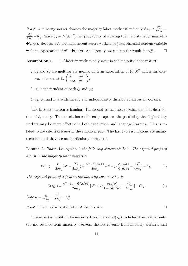
Lemma 2. Under Assumption 1, the following statements hold. The expected profit of

a firm in the majority labor market is

E(πld) =nd

2mld

(αd − βdld

4mld

) +nm · Φ(µ/σ)

2mld

[αm − ρsφ(µ/σ)Φ(µ/σ)

− βmld

4mld

]− Cld . (8)

The expected profit of a firm in the minority labor market is

E(πlm) =nm · (1− Φ(µ/σ))

2mlm

[αm + ρsφ(µ/σ)

1− Φ(µ/σ)− βm

lm

4mlm

]− Clm . (9)

Note µ =βm

lm

8mlm− βm

ld

8mld

− θmld.

Proof. The proof is contained in Appendix A.2.

The expected profit in the majority labor market E(πld) includes three components:

the net revenue from majority workers, the net revenue from minority workers, and

11

the fixed cost of operating a firm. Notice the additional component −ρs φ(µ/σ)Φ(µ/σ)

that

represents an adjustment due to the selection of high ability minority workers into the

majority labor market.7 A similar interpretation applies to the expected profit in the

minority labor market.

The necessary condition for equilibrium are that firms in both labor markets earn

zero profits. In fact, the two zero profits conditions completely characterize the number

of firms and other endogenous variables, such as wages, in equilibrium. However, the mi-

nority labor market may not exist. Multiple equilibria where both labor market exist are

also possible. Any comparative statics necessarily hinge upon restrictive assumptions.

Proposition 1. If (1) conditions in Assumption 1 hold, (2) the model parameters are

such that there is at least one pair of (mld ,mlm), where mld > 0 and mlm > 0, (3) ρ = 0,

and (4) the Jacobian J of the zero profit conditions evaluated at the equilibrium pair

(mld ,mlm) is negative definite, the following comparative statics hold for the equilibrium

pair (mld ,mlm).

mld mlm

Majority Population (nd) + –Minority Population (nm) ? ?

Language Learning Cost (θmld

) – +Communication Cost #1 (βd

ld) – +

Communication Cost #2 (βmld

) – +Communication Cost #3 (βm

lm) + –

Firm Operating Cost #1 (Cld) – +Firm Operating Cost #2 (Clm) + –

Majority Productivity (αd) + –Minority Productivity (αm) ? ?

Proof. See Appendix A.3 for detailed derivation.

The first assumption is familiar. The second states that there are two submarkets in

equilibrium. This is the case when it is appropriate to discuss the comparative statics.

7Suppose high ability workers tend to incur less costs in learning a language and to have higherproductivity. This means ψi and ξi are negatively correlated or ρ < 0. This in turn implies that theadjustment term is positive, meaning the firm currently earns more net revenue from minority workersthan the case when there is no selection.

12

Zero Profit CurveMajority:Before

Zero Profit CurveMajority:After

Zero Profit CurveMinorityBefore and After

010

020

030

040

0Nu

mbe

r of M

inor

ity F

irms

200 400 600 800 1000Number of Majority Firms

Majority Population Increase by 20%

Zero Profit CurveMajoriy:Before

Zero Profit CurveMajority:After

Zero Profit CurveMinority:Before

Zero Profit CurveMinority:After

200

250

300

350

400

Num

ber o

f Min

ority

Firm

s

480 500 520 540 560 580Number of Majority Firms

Minority Population Increase by 40%

Figure 2: Number of Firms and the Language Group Populations

The third assumption is added to simplify the analysis. I will consider non-zero ρ in

the following numerical example. The last assumption selects an equilibrium in which

the numbers of firms and the equilibrium profits change in the opposite direction. This

equilibrium is stable in the sense that small shocks to profits do not lead to divergence

from the equilibrium.8

The basic parameter setup of the numerical example is as follows: nd = 10000,

nm = 5000, αd = αm = 10000, βdld

= βmlm

= 15000, βmld

= 18000, ρ = −0.9, s = 5000,

σ = 10, θmld

= 20, and Cld = Clm = 100000. Note that I allow ρ 6= 0 in this numerical

exercise.

Figure 2 to Figure 4 show the pairs of (mld ,mlm) that satisfy the two zero profit

conditions. The thick solid line represents the zero profit condition of the majority

market. The thin solid line corresponds to the zero profit condition of the minority

market. The intersection of the two is therefore an equilibrium.9

8Suppose firms enter if there are positive profits and exit if the profits are negative. A necessary andsufficient condition for the stability of the equilibrium is that (1) J(1, 1) + J(2, 2) < 0 and (2)|J | > 0.These two conditions are implied by assumption (4) of Proposition 1.

9There are in fact multiple solutions. However, the one shown in this figure is the only stablesolution.

13

Zero Profit CurveMajority:Before

Zero Profit CurveMajority:After

Zero Profit CurveMinorityBefore and After

010

020

030

040

0Nu

mbe

r of M

inor

ity F

irms

200 400 600 800 1000Number of Majority Firms

Majority Workers’ Productivity Increase by 20%

Zero Profit CurveMajoriy:Before

Zero Profit CurveMajority:After

Zero Profit CurveMinority:Before

Zero Profit CurveMinority:After

200

250

300

350

400

Num

ber o

f Min

ority

Firm

s

480 500 520 540 560 580Number of Majority Firms

Minority Workers’ Productivity Increase by 40%

Figure 3: Number of Firms and the Average Productivities

The left graph of Figure 2 shows the comparative statics with respect to majority

population. As the majority population increases, the zero profit curve of the majority

market shifts outward, while that of the minority market remains unchanged. As a

result, the number of majority firms increases, while that of minority firms decreases.

This happens because the matching quality in the majority labor market improves as

majority population increases. More firms enter this labor market. At the same time,

more minority workers enter the majority market in search of higher wages. Profits in

in the minority labor market decrease. Firms exit the minority labor market.

The second graph of Figure 2 shows the comparative statics with respect to the

minority population. Both zero profit curves shift outward. The number of minority

firms increases significantly, while that of majority firms decreases slightly. Although

Proposition 1 does not have a definite answer about it, this example indicates that the

number of minority firms is more sensitive to minority population.

Figure 3 illustrates the comparative statics with respect to average productivities of

the two groups, namely αd and αm. The results are similar to those in Figure 2. The

economic mechanism is also similar. Again, the number of minority firms seems to be

14

Zero Profit CurveMajoriy:BeforeZero Profit Curve

Majority:After

Zero Profit CurveMinority:Before

Zero Profit CurveMinority:After

200

220

240

260

280

300

Num

ber o

f Min

ority

Firm

s

450 500 550 600Number of Majority Firms

Language Learning Cost Increase by 20%

Zero Profit CurveMajority:Before

Zero Profit CurveMajority:After

Zero Profit CurveMinority:Before

Zero Profit CurveMinority:After

200

220

240

260

Num

ber o

f Min

ority

Firm

s

500 520 540 560Number of Majority Firms

Minority Workers’ Communication Costsin Majority Market Increase by 40%

Figure 4: Number of Firms and the Language Learning and Communication Costs

more sensitive to changes in the average productivity of αm.

Figure 4 shows the comparative statics with respect to θmld

and βmld

. As these language

related costs increase, the number of majority firms decrease and the number of minority

firms increase. The increase in those costs discourages minority workers from entering

the majority market. The matching quality and potential profit in the minority market

increase, so more firms enter the minority market. On the other hand, the profit in the

majority market diminishes, and firms exit from the majority market.

Comparative statics with respect to other parameters follow the same line of thought.

It is also straightforward but tedious to generalize the two-ethnic-group, two-labor-

submarket framework into a multi-ethnic-group and multi-labor-submarket model. Ap-

pendix B contains a sketch of such a generalization. The comparative statics become

messier but the message is still the same.

2.6 Empirical Implications

In this section, I will discuss the empirical implications of the theory. The first key

implication is summarized in the following proposition.

15

Proposition 2. There are two types of wage gaps: the Within-labor-market Wage Gap

and the Within-language-group Wage Gap. Under Assumption 1, the Within-labor-

market Wage Gap can be expressed as

E(W dld−Wm

ld) =

1

2[αd − αm +

βmld

4mld

− βdld

4mld

]. (10)

Under Assumption 1, the Within-language-group Wage Gap can be expressed as

E(Wmld−Wm

lm) =1

2[

βmlm

4mlm

− βmld

4mld

]. (11)

Proof. These two expressions are directly implied by equation (6) and assumption 1.

Note that W dld

is the wage earned by a majority group worker. The wage of a

minority worker who works in the majority labor market is denoted as Wmld

. The wage

of a minority worker in the minority labor market is denoted as Wmlm

. I will test the

existence of the two wage gaps empirically.

The second key implication is the comparative statics of the wages with respect to

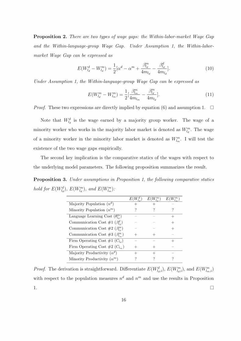
the underlying model parameters. The following proposition summarizes the result.

Proposition 3. Under assumptions in Proposition 1, the following comparative statics

hold for E(W dld), E(Wm

ld), and E(Wm

lm):

E(W dld

) E(Wmld

) E(Wmlm

)Majority Population (nd) + + –Minority Population (nm) ? ? ?

Language Learning Cost (θmld

) – – +Communication Cost #1 (βd

ld) – – +

Communication Cost #2 (βmld

) – – +Communication Cost #3 (βm

lm) + + –

Firm Operating Cost #1 (Cld) – – +Firm Operating Cost #2 (Clm) + + –

Majority Productivity (αd) + + –Minority Productivity (αm) ? ? ?

Proof. The derivation is straightforward. Differentiate E(W dld,i), E(Wm

ld,i), and E(Wmlm,i)

with respect to the population measures nd and nm and use the results in Proposition

1.

16

Notice the link between Proposition 3 and Proposition 1. It is easy to confirm that

both E(W dld) and E(Wm

ld) move positively with mld and that E(Wm

lm) moves positively

with mlm . Therefore, Figure 2 to Figure 4 provide visual help to understand the results

of Proposition 3.

One may notice the absence of the supply effect on wages. Indeed, this comes from

the assumption of a fixed output price. If the output demand is downward sloping, the

labor demand curve is likely to be downward sloping, so the supply effect matters. In

the model, I focus on the market thickness effect which leads to a upward sloping labor

demand curve. Whether the supply effect is more important than the market thickness

effect is a subject of our empirical analysis.

The results in Proposition 3 are important because the effects of many immigration

policies can be traced back to changes in the parameters of the model. I have classified

the underlying parameters into several categories: the populations of the two language

groups, the language-related costs, the fixed costs of starting a business in different

labor markets, and the productivities of workers from different language groups. The

framework in this paper is hence a good starting point to evaluate various immigration

policies.

It is sometimes suggested that the government should encourage new immigrants

to settle in small cities where they can better mingle into the society. This decreases

the minority population in big cities, which in turn reduces wages in the minority labor

market and increases wages in the majority labor market. At least in the short run,

the workers in the ethnic enclaves will bear the cost. The workers in the majority labor

market may be better off or worse off (See Figure 2).

It has also been widely discussed that the government should facilitate the recogni-

tion of overseas qualifications earned by new immigrants. This policy is equivalent to

increasing perceived αm by employers. Minority workers in ethnic enclaves benefit from

such a policy, while worker in the majority market can either benefit or suffer from such

17

a policy (See Figure 3). Policies that reduce workplace discrimination have the same

effects.

Another prominent policy is to subsidize language learning, for example setting up

free language lessons or subsidizing community activities. This policy reduces θmld

and

βmld

. Again, those who remain in the ethnic enclaves are worse off, while those who leave

the ethnic enclaves and the majority workers are better off (See Figure 4).

There are also policies that help immigrants to start small businesses. They reduce

the cost of setting up a firm. The effects depend on whether those entrepreneurs set

up businesses in the majority market or the minority market. If the latter is the case,

workers in the ethnic enclave will benefit, while those outside the enclave will suffer.

I have shown that the language theory of labor market segmentation has rich impli-

cations. The test of the theory is however limited due to data availability. In the dataset

I use, there are good measures for populations nd and nm. There are also proxies for θmld

and βmld

. The language distance measure proposed by Chiswick and Miller (2004) is a

good candidate. Age at immigration is another.10 Unfortunately, some parameters are

difficult to measure. These include the costs of operation a firm and the within-group

communication costs. Therefore, we focus on the existence of the two types of wage

gaps and the comparative statics with respect to populations.

3 Data

The main source of data is the 2001 Census of Canada Public Use Microdata File

(henceforth 2001 Canada PUMF or PUMF) on individuals. This dataset is a 2.7%

sample of the Canadian population. Because this paper is only interested in urban

workers, I exclude all individuals who do not reside in a Census Metropolitan Area

(CMA) from our analysis. This exclusion reduces the number of observations to 496,611,

representing a population of 18,348,790.

10We also need a variable to differentiate between θmld

and βmld

. This is called an ‘exclusion restriction’.See Section 4.1.1 for details.

18

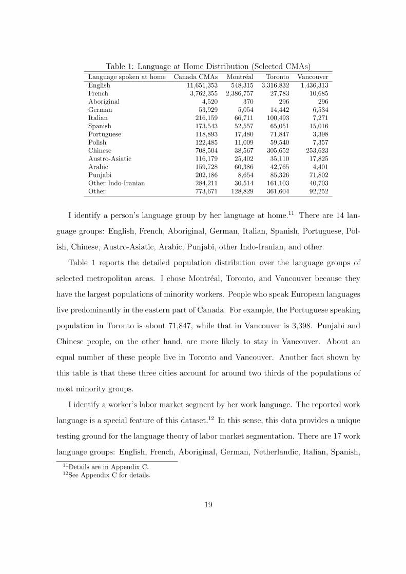
Table 1: Language at Home Distribution (Selected CMAs)Language spoken at home Canada CMAs Montreal Toronto VancouverEnglish 11,651,353 548,315 3,316,832 1,436,313French 3,762,355 2,386,757 27,783 10,685Aboriginal 4,520 370 296 296German 53,929 5,054 14,442 6,534Italian 216,159 66,711 100,493 7,271Spanish 173,543 52,557 65,051 15,016Portuguese 118,893 17,480 71,847 3,398Polish 122,485 11,009 59,540 7,357Chinese 708,504 38,567 305,652 253,623Austro-Asiatic 116,179 25,402 35,110 17,825Arabic 159,728 60,386 42,765 4,401Punjabi 202,186 8,654 85,326 71,802Other Indo-Iranian 284,211 30,514 161,103 40,703Other 773,671 128,829 361,604 92,252

I identify a person’s language group by her language at home.11 There are 14 lan-

guage groups: English, French, Aboriginal, German, Italian, Spanish, Portuguese, Pol-

ish, Chinese, Austro-Asiatic, Arabic, Punjabi, other Indo-Iranian, and other.

Table 1 reports the detailed population distribution over the language groups of

selected metropolitan areas. I chose Montreal, Toronto, and Vancouver because they

have the largest populations of minority workers. People who speak European languages

live predominantly in the eastern part of Canada. For example, the Portuguese speaking

population in Toronto is about 71,847, while that in Vancouver is 3,398. Punjabi and

Chinese people, on the other hand, are more likely to stay in Vancouver. About an

equal number of these people live in Toronto and Vancouver. Another fact shown by

this table is that these three cities account for around two thirds of the populations of

most minority groups.

I identify a worker’s labor market segment by her work language. The reported work

language is a special feature of this dataset.12 In this sense, this data provides a unique

testing ground for the language theory of labor market segmentation. There are 17 work

language groups: English, French, Aboriginal, German, Netherlandic, Italian, Spanish,

11Details are in Appendix C.12See Appendix C for details.

19

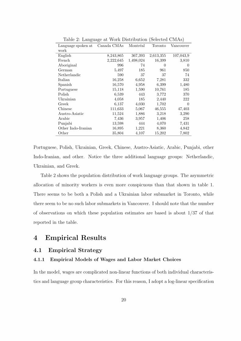
Table 2: Language at Work Distribution (Selected CMAs)Language spoken atwork

Canada CMAs Montreal Toronto Vancouver

English 8,243,865 367,393 2,613,355 107,043,9French 2,222,645 1,498,024 16,399 3,810Aboriginal 996 74 0 0German 5,497 185 961 850Netherlandic 590 37 37 74Italian 16,258 6,652 7,281 332Spanish 16,570 4,958 6,399 1,480Portuguese 15,118 1,590 10,761 185Polish 6,539 443 3,772 370Ukrainian 4,058 185 2,440 222Greek 6,137 4,030 1,702 0Chinese 111,633 5,067 46,555 47,403Austro-Asiatic 11,524 1,886 3,218 3,290Arabic 7,436 3,957 1,406 258Punjabi 13,598 444 4,070 7,431Other Indo-Iranian 16,895 1,221 8,360 4,842Other 35,804 4,107 15,202 7,802

Portuguese, Polish, Ukrainian, Greek, Chinese, Austro-Asiatic, Arabic, Punjabi, other

Indo-Iranian, and other. Notice the three additional language groups: Netherlandic,

Ukrainian, and Greek.

Table 2 shows the population distribution of work language groups. The asymmetric

allocation of minority workers is even more conspicuous than that shown in table 1.

There seems to be both a Polish and a Ukrainian labor submarket in Toronto, while

there seem to be no such labor submarkets in Vancouver. I should note that the number

of observations on which these population estimates are based is about 1/37 of that

reported in the table.

4 Empirical Results

4.1 Empirical Strategy

4.1.1 Empirical Models of Wages and Labor Market Choices

In the model, wages are complicated non-linear functions of both individual characteris-

tics and language group characteristics. For this reason, I adopt a log-linear specification

20

of wages.

ln W dld,i = Xiγ

d + Gδd + εdi , (12)

ln Wmld,i = Xiγ

mld

+ Gδmld

+ εmld,i, (13)

ln Wmlm,i = Xiγ

mlm + Gδm

lm + εmlm,i. (14)

Log wages are measured as the logarithm of workers’ hourly earnings. Notice the sub-

script and superscript associated with model coefficients and error terms.

Xi is a vector of individual characteristics: education, experience, experience squared,

sex, marital status, interaction of sex and marital status, a dummy indicating whether

a person immigrate after age 19, and occupation fixed effects. ‘Age at immigration’

dummy is included to control for the adaptation of immigrants. It may also correlates

with language skills. Occupation dummies are included to differentiate this theory from

a theory in which minority workers and majority workers sort into different occupations

(Card, 2001).

G is a vector of group-wide variables, which includes the majority population in the

city in which the worker lives, the population of the worker’s language group in the city,

and possible other variables. These variables are omitted in testing the two wage gaps.

They are included in testing the comparative statics.

For a minority worker, the choice of labor market is based on a comparison of net

wages. Similar to equation (7), I define the net wage gain from entering the majority

labor market as

Ii = ln Wmld,i − ln Wm

lm,i − θmld,i − ψi = Xiλ1 + Ziλ2 + Gλ3 + ei. (15)

Note the additional vector Zi, the exclusion restriction I impose on the wage equation.

The error term ei is a normal random variable.

One possible variable for the exclusion restriction is a measure of distance between

a minority language and English proposed by Chiswick and Miller (2004). They use

21

the scores of English as a Second Language students as the measure of distance be-

tween English and other languages. However, this variable may not be a valid exclusion

restriction because it is correlated with a person’s ability to learn the tacit aspects of

English, too. We know that this ability affects wages.

I instead use the interaction between the language score and a worker’s age at im-

migration dummy as the exclusion restriction. Suppose there are four immigrants. Two

come from Ireland, where exposure to English is prevalent. One of them immigrated at

the age of 5 and the other at 25. The other two have the same immigration age profile,

but they come from Mexico, where exposure to English is limited.

The two Irish differ in terms of their tacit knowledge of English and their social

networks. The two Mexicans, however, differ not only in terms of their tacit knowledge of

English and their social networks, but also in their knowledge of explicit forms of English.

Therefore, subtracting the difference between the two Irish from the difference between

the two Mexicans gives a measure of the explicit form of English. This subtraction can

be done mechanically by adding an interaction between immigration age dummy and

language score.

In the majority labor market, all the workers have to master the explicit forms of

the majority language. The measure of the explicit forms of a language should not enter

the wage equation. However, the language learning cost is directly determined by the

difficulty in learning the explicit forms of English. Therefore, the interaction between

immigration age and language score is a valid exclusion restriction.13

4.1.2 Within-labor-market Wage Gap

Recall that the Within-labor-market Wage Gap is the wage difference between a ma-

jority worker and a minority worker in the majority labor market. Define lnWld,i as

Di ln W dld,i + (1 − Di) ln Wm

ld,i, where Di = 1 indicates a majority worker and Di = 0

13I do not have similar language scores for French. However, when I model workers’ labor market orwork language choice in Quebec, I do need such a score. I assume that a minority individual’s Frenchscore is the same as her English score.

22

indicates a minority worker. If E(Xi|G) = E(Xi), we can omit group wide variables in

equation (12) and (13) and write

E(ln Wld,i|Xi, Di) = µ0 + Di · µ1 + Xiµ2 + Di(Xi − E(X))µ3 + (1−Di)φ(.)

Φ(.)µ4. (16)

Under standard conditions in the treatment effect literature, we can estimate the Within-

labor-market Wage Gap by running the above regression over all workers in the majority

labor market.14 The estimated wage gap is µ1 for a worker with average characteristics

E(X). The estimated wage gap is µ1 + (Xi −E(X))µ3 for a worker with characteristic

Xi, which includes education, work experience, and other individual characteristics.

The inverse Mill’s ratio term φ(.)Φ(.)

is included because only minority workers who

choose the majority labor market are in the sample. It is constructed from equation

(15) with group-wide variables omitted.

It is possible that the above estimated wage gap is a reflection of discrimination.

To differentiate from such an alternative, I add worker’s visible minority status Vi, an

interaction Li×Vi, and the interaction between the status and the demeaned individual

characteristics Vi(Xi−E(X)) to the previous regression. Vi = 1 indicates that a worker

is a visible minority and Vi = 0 indicates otherwise.

4.1.3 Within-language-group Wage Gap

Recall that Within-language-group Wage Gap is the wage difference between two mi-

nority workers who work in different labor markets. Define lnWmi as Li ln Wm

ld,i + (1 −Li) ln Wm

lm,i. Li indicates the worker’s labor market status, which equals 1 if it is the

majority labor market but equals 0 otherwise. If E(Xi|G) = E(Xi), we can omit group

wide variables in equation (13) and (14) and write

E(ln Wmi |Xi, Li) = µ0 + Liµ1 + Xiµ2 + Li(Xi − E(X))µ3

+ (1− Li)φ(.)

1− Φ(.)µ4 + Li

φ(.)

Φ(.)µ5. (17)

14See Wooldridge (2002) for a complete discussion of the conditions underlying the use of switchingregression in order to estimate Average Treatment Effect.

23

We can estimate the Within-language-group Wage Gap by running the above regression

over all minority workers.15 The estimated wage gap is µ1 for a worker with average

characteristics E(X). The estimated wage gap is µ1 + (Xi−E(X))µ3 for a worker with

characteristic Xi.

In the sample, we only observe workers who have made their labor market choices.

I follow the framework of Lee (1982) in addressing this self-selection problem. The

difference is that I include both selection correction terms φ(.)Φ(.)

and φ(.)1−Φ(.)

in one switching

regression instead of running two separate regressions. The selection correction terms

are both constructed from equation (15), with the group-wide variables omitted.

It is also possible that the above estimated wage gap is because of the different

discriminative treatment of minorities across labor markets. To differentiate from such

alternatives, I add the worker’s visible minority status Vi and the interaction between

the visible minority status and the demeaned individual characteristics Vi(Xi−E(X)) to

the previous regression. Moreover, the interaction between visible minority status and

labor market status Li×Vi is also added to control for different degrees of discrimination

in the two labor markets.

4.1.4 Tests of Comparative Statics

In this section, I include population measures to test their marginal effects on individual

wages. I again adopt the method of Lee (1982) to address the selection issues. I run

two separate wage regressions for minority workers in the majority labor market and

minority workers in the minority labor market, respectively.

E(lnWmld,i|Xi, G, nm, nd, Li = 1) = Xiµ1d + Gµ2d + µ3d lnnm + µ4d lnnd +

φ(.)Φ(.)

µ5d (18)

E(lnWmlm,i|Xi, G, nm, nd, Li = 0) = Xiµ1m+Gµ2m+µ3m lnnm+µ4m lnnd+

φ(.)1− Φ(.)

µ5m. (19)

I include in Xi the individual characteristics as well as the worker’s visible minority sta-

tus and its interactions with demeaned education, experience, and experience squared.

15Again, see Wooldridge (2002) for the conditions needed.

24

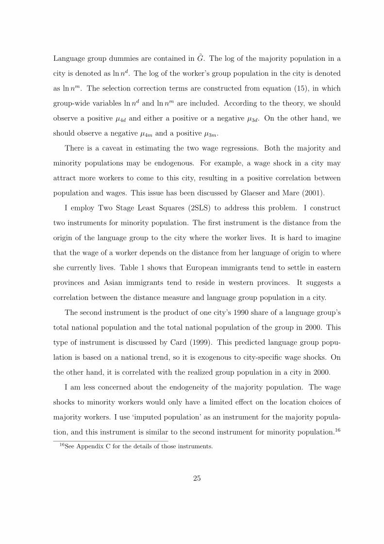
Language group dummies are contained in G. The log of the majority population in a

city is denoted as ln nd. The log of the worker’s group population in the city is denoted

as ln nm. The selection correction terms are constructed from equation (15), in which

group-wide variables ln nd and ln nm are included. According to the theory, we should

observe a positive µ4d and either a positive or a negative µ3d. On the other hand, we

should observe a negative µ4m and a positive µ3m.

There is a caveat in estimating the two wage regressions. Both the majority and

minority populations may be endogenous. For example, a wage shock in a city may

attract more workers to come to this city, resulting in a positive correlation between

population and wages. This issue has been discussed by Glaeser and Mare (2001).

I employ Two Stage Least Squares (2SLS) to address this problem. I construct

two instruments for minority population. The first instrument is the distance from the

origin of the language group to the city where the worker lives. It is hard to imagine

that the wage of a worker depends on the distance from her language of origin to where

she currently lives. Table 1 shows that European immigrants tend to settle in eastern

provinces and Asian immigrants tend to reside in western provinces. It suggests a

correlation between the distance measure and language group population in a city.

The second instrument is the product of one city’s 1990 share of a language group’s

total national population and the total national population of the group in 2000. This

type of instrument is discussed by Card (1999). This predicted language group popu-

lation is based on a national trend, so it is exogenous to city-specific wage shocks. On

the other hand, it is correlated with the realized group population in a city in 2000.

I am less concerned about the endogeneity of the majority population. The wage

shocks to minority workers would only have a limited effect on the location choices of

majority workers. I use ‘imputed population’ as an instrument for the majority popula-

tion, and this instrument is similar to the second instrument for minority population.16

16See Appendix C for the details of those instruments.

25

4.1.5 Issues about the Data

My conceptual framework and the data are somewhat incompatible. In the data, there

are several language groups and several potential labor markets in a city. In the theory,

however, there are only two language groups and two labor markets. I extend the model

to multi-group and multi-market setting in Appendix B. In this setting changes in one

minority labor market may affect wages other minority labor markets. I call this the

‘ripple effect’.

The ‘ripple effect’ does not matter much if there is a single group that has a much

larger population than the populations of all the other groups. However, it matters if

there are two groups that are similar in size: changes in the slightly smaller language

group may affect other smaller groups. I suspect that Montreal and Ottawa are two

examples. To alleviate this concern, I carry out the analysis on a subsample of cities,

excluding cities in Quebec and the city of Ottawa.

A related problem may arise due to the bilingualism policy in Canada. When there

are a lot of people who can communicate in both English and French, the boundaries

between labor markets are no longer clear. In addition, the fact that there are certain

advantages to become bilingual, such as qualifying for government jobs, complicates the

analysis. Empirically, I alleviate the problem by simply excluding the English group in

Quebec and the French group outside Quebec from the analysis.

4.2 Regression Results

4.2.1 Labor Market Choice

The labor market choice is modeled in equation (15). Table 3 reports the estimates.

There are two subsamples: workers in all Canadian CMAs and workers in CMAs out-

side Quebec and Ottawa. The estimates in this table are used to construct selection

correction terms in wage regressions later on.

In general, higher education leads to higher probability of selecting the majority

26

Table 3: Labor Market Choices of Minority WorkersAll CMAs CMAs outside Quebec

Model 1 Model 2 Model 3 Model 1 Model 2 Model 3Education 0.0695a 0.0694a 0.0711a 0.0712a 0.0708a 0.0733a

(0.0019) (0.0019) (0.0020) (0.0021) (0.0021) (0.0021)

Age -0.0058a -0.0055a -0.0054a -0.0053a -0.0050a -0.0047a

(0.0006) (0.0006) (0.0006) (0.0006) (0.0006) (0.0006)

Sex (Female=1) -0.0054 -0.0029 0.0007 -0.0091 -0.0062 -0.0007(0.0124) (0.0124) (0.0125) (0.0132) (0.0132) (0.0133)

Immigrate after age 19 -0.2695a -1.1202a -1.1230a -0.2867a -1.1882a -1.2010a

(0.0153) (0.0761) (0.0765) (0.0163) (0.0816) (0.0821)

Language Score (LS) 0.5083a 0.2442a 0.1931a 0.6080a 0.3281a 0.2441a

(0.0191) (0.0299) (0.0307) (0.0206) (0.0321) (0.0331)

LS*Imm. after age 19 0.4369a 0.4394a 0.4659a 0.4732a

(0.0382) (0.0384) (0.0412) (0.0415)

Log own group population -0.0700a -0.1041a

(0.0073) (0.0080)

Log majority population 0.0612a 0.1202a

(0.0149) (0.0159)

Intercept -0.8102a -0.2961a -0.3213b -1.0171a -0.4725a -0.8861a

(0.0519) (0.0688) (0.1564) (0.0554) (0.0736) (0.1648)

N 50,436 50,436 50,436 45,100 45,100 45,100Pseudo R2 0.0508 0.0531 0.0555 0.0572 0.0598 0.0638

The choice variable is the worker’s language at work. It equals 1 if it is English (or French in Quebec), 0 otherwise.Minority workers are those whose home languages are neither English nor French. a significance level of 1%. b

significance level of 5%. c significance level of 10%. Standard errors are in parentheses.

labor market. Older people are less likely to enter the majority labor market. Those

who immigrated after age 19 are less likely to choose the majority labor market. Female

workers seem to be less likely to work in the majority labor market, though the difference

is not statistically significant.

For all CMAs, the effect of language score has the expected positive sign. Recall that

the language score is higher when the distance between two languages is smaller. The

effect of language score is stronger for those who immigrated after age 19 as indicated

by the positive coefficient before the interaction term. Based on Model 3, the size of the

majority population in the city increases the probability of a worker choosing the major-

ity labor market. The person’s own group’s population, however, has a negative effect.

Those results are consistent with the language theory of labor market segmentation.

27

The results for CMAs outside Quebec are similar.

4.2.2 Within-labor-market Wage Gap

In this section, I show the existence of the Within-labor-market Wage Gap. Remember it

is the wage difference between a majority worker and a minority worker in the majority

labor market. The sample includes all workers who speak English at work outside

Quebec or French in Quebec. I exclude workers who speak English at home in Quebec

and workers who speak French at home outside Quebec. This exclusion alleviates the

concern about the bilingualism policy.

Table 4 shows the results, first, for all CMAs and, secondly, for CMAs outside

Quebec and Ottawa, respectively. The exclusion of the CMAs in Quebec and Ottawa is

to address the concern about the ‘ripple effect’. Since the results for the two subsamples

are fairly similar, I discuss the results for all CMAs only.

Model 1 is the starting point. Since I do not include age at immigration dummy, I

am comparing one person who was born in Canada versus another person who was born

in another country. I find that a majority worker, who has the average education and

experience of the sample, earns 13.9% more than her minority counterpart. In addition,

the former gets more for one additional year of education and work experience. The

regressors, such as education, experience, and others, all have the expected signs.

Model 2 controls for age at immigration dummy and occupation fixed effects. Es-

sentially, I am comparing two individuals who were both born in Canada and who have

the same occupation. I find that a majority worker does not necessarily earn more than

a minority worker, if both have the average education and experience of the sample.

The estimated gap is 1.6%, which is not statistically significant. However, the different

payoffs to education and experience remain significant.

Model 3 includes additionally the inverse Mill’s ratio to correct for the self-selection

of minority workers into the majority labor market. Presumably, this specification will

yield more reliable estimates. Notice that the wage gap is reduced to -0.7%, which is

28

Table 4: Within-labor-market Wage Gap Ignoring DiscriminationSpecification All CMAs CMAs outside Quebec

Model 1 Model 2 Model 3 Model 1 Model 2 Model 3Majority group (Di = 1) 0.1393a 0.0163 -0.0074 0.1398a -0.0009 -0.0142

(0.0326) (0.0685) (0.0758) (0.0357) (0.0686) (0.0747)

Education 0.0629a 0.0404a 0.0355a 0.0600a 0.0392a 0.0347a

(0.0042) (0.0033) (0.0047) (0.0046) (0.0035) (0.0051)

Experience 0.0146a 0.0180a 0.0191a 0.0142a 0.0177a 0.0186a

(0.0023) (0.0021) (0.0022) (0.0024) (0.0022) (0.0023)

Experience sqd. -0.0001b -0.0002a -0.0002a -0.0001c -0.0002a -0.0002a

(0.0001) (0.0000) (0.0000) (0.0001) (0.0001) (0.0001)

(Demeaned Educ)*Di 0.0225a 0.0125a 0.0172a 0.0222a 0.0119a 0.0162a

(0.0048) (0.0037) (0.0049) (0.0053) (0.0041) (0.0052)

(Demeaned Exper)*Di 0.0233a 0.0141a 0.0130a 0.0247a 0.0156a 0.0146a

(0.0030) (0.0028) (0.0028) (0.0032) (0.0031) (0.0030)

(Demeaned Exper2)*Di -0.0004a -0.0003a -0.0003a -0.0005a -0.0003a -0.0003a

(0.0001) (0.0001) (0.0001) (0.0001) (0.0001) (0.0001)

Sex (Female=1) -0.1106a -0.1145a -0.1144a -0.1187a -0.1180a -0.1179a

(0.0087) (0.0075) (0.0075) (0.0109) (0.0093) (0.0093)

Married 0.1866a 0.1652a 0.1655a 0.1888a 0.1659a 0.1662a

(0.0102) (0.0091) (0.0091) (0.0119) (0.0106) (0.0106)

Sex*Married -0.0971a -0.0948a -0.0949a -0.0907a -0.0875a -0.0876a

(0.0096) (0.0107) (0.0107) (0.0109) (0.0115) (0.0116)

Language score 0.0298 -0.0101 0.0452 0.0033(0.0606) (0.0630) (0.0632) (0.0657)

Immigrate after age 19 -0.1231a -0.1168a -0.1285a -0.1227a

(0.0109) (0.0122) (0.0132) (0.0160)

Inverse Mill’s ratio -0.1681 -0.1504(0.1251) (0.1335)

Intercept 1.4971a 2.2430a 2.4359a 1.5473a 2.2639a 2.4492a

(0.0619) (0.1211) (0.1575) (0.0650) (0.1280) (0.1635)

Occupation dummies No Yes Yes No Yes Yes

N 176651 176610 176610 142812 142772 142772R2 0.1190 0.1452 0.1452 0.1200 0.1460 0.1460

The dependent variables are log hourly wages. The inverse Mill’s ratio is computed using model 2 of table 3 for allCMAs and CMAs outside Quebec, respectively. a significance level of 1%. b significance level of 5%. c significance levelof 10%. Standard errors are in parentheses. The regression error terms are clustered by individual language groupwithin a CMA.

insignificant. Furthermore, the estimated return to education or experience increases

compared with that of Model 2. The difference in payoff to education and experience

remains statistically significant.

The insignificance of the estimated wage gap after selection correction is puzzling.

29

We expect that minority workers with higher ability are more likely to enter the majority

labor market. Therefore, the uncorrected wage gap is an underestimate of the real wage

gap. This story presumes a negative correlation between a worker’s productivity and

her language learning cost.

However, some unobservable characteristics can also induce a positive correlation

between language learning cost and productivity, which in turn implies the result in

table 4. For example, those with smaller social networks tend to enter the majority

labor market because their social networks present fewer opportunities in the minority

labor market. On the other hand, the productivity of those workers is also lower.

Therefore, the uncorrected wage gap is an overestimate of the real gap.

Table 5 controls for discrimination based on a worker’s appearance. I add ‘visible

minority status’ of a worker, its interaction with language group dummy, and its inter-

actions with demeaned education, experience, and experience squared. I will again only

discuss the results for all CMAs since the results for CMAs outside Quebec are similar.

Model 1, Model 2, and Model 3 have similar interpretations to previous findings.

The difference is that the two workers I am comparing should have the same visible

minority status. Since I include interaction between Di and Vi, the estimated wage gap

is different for people with different visible minority status. The message from table 5 is

essentially the same. The estimated wage gap is not always significant, but the rewards

for education and experience are quite different across the two language groups. I also

find that the estimated wage gap is larger for visible minorities. The return to education

and experience for visible minorities is also lower.

In summary, the results in tables 4 and 5 are persistent. First, I find a strong

difference in returns for education and experience across the language groups. This

supports the existence of a Within-labor-market Wage Gap. Second, the estimated wage

gap for a worker with average characteristics can be positive or negative, depending on

which conceptual comparison we are making. In my view, Model 3’s estimate represents

30

Table 5: Within-labor-market Wage Gap Considering DiscriminationSpecification All CMAs CMAs outside Quebec

Model 1 Model 2 Model 3 Model 1 Model 2 Model 3Majority group (Di = 1) 0.0687c 0.0631 0.0386 0.0676 0.0506 0.0373

(0.0386) (0.0666) (0.0702) (0.0418) (0.0683) (0.0716)

Visible minority (Vi = 1) -0.1338a -0.1120a -0.1111a -0.1396a -0.1119a -0.1111a

(0.0396) (0.0244) (0.0245) (0.0412) (0.0266) (0.0268)

Interaction Di ∗ Vi 0.028 0.0616b 0.0583b 0.0302 0.0587c 0.0557c

(0.0428) (0.0280) (0.0284) (0.0476) (0.0327) (0.0331)

Education 0.0624a 0.0374a 0.0325a 0.0596a 0.0361a 0.0319a

(0.0045) (0.0042) (0.0051) (0.0044) (0.0041) (0.0051)

Experience 0.0222a 0.0213a 0.0223a 0.0222a 0.0213a 0.0222a

(0.0033) (0.0030) (0.0032) (0.0036) (0.0032) (0.0034)

Experience sqd. -0.0002a -0.0002a -0.0002a -0.0002a -0.0002a -0.0002a

(0.0001) (0.0001) (0.0001) (0.0001) (0.0001) (0.0001)

(Demeaned Educ)*Di 0.0230a 0.0152a 0.0200a 0.0224a 0.0145a 0.0187a

(0.0046) (0.0039) (0.0051) (0.0043) (0.0037) (0.0051)

(Demeaned Exper)*Di 0.0164a 0.0113a 0.0103a 0.0177a 0.0126a 0.0117a

(0.0039) (0.0034) (0.0036) (0.0043) (0.0038) (0.0040)

(Demeaned Exper2)*Di -0.0003a -0.0002a -0.0002a -0.0004a -0.0003a -0.0003a

(0.0001) (0.0001) (0.0001) (0.0001) (0.0001) (0.0001)

(Demeaned Educ)*Vi 0.0033 0.0036 0.0034 0.0034 0.004 0.0037(0.0055) (0.0050) (0.0050) (0.0054) (0.0050) (0.0050)

(Demeaned Exper)*Vi -0.0088b -0.0054 -0.0053 -0.0092b -0.0061 -0.006(0.0040) (0.0038) (0.0038) (0.0044) (0.0040) (0.0041)

(Demeaned Exper2)*Vi 0.0001 0.0000 0.0000 0.0001 0.0001 0.0001(0.0001) (0.0001) (0.0001) (0.0001) (0.0001) (0.0001)

Language score -0.0604 -0.1006 -0.048 -0.0883(0.0624) (0.0669) (0.0671) (0.0711)

Immigrate after age 19 -0.0930a -0.0859a -0.0963a -0.0900a

(0.0135) (0.0136) (0.0139) (0.0143)

Inverse Mill’s ratio -0.1732 -0.1485(0.1238) (0.1259)

Intercept 1.4973a 2.4711a 2.6661a 1.5458a 2.4945a 2.6734a

(0.0904) (0.1417) (0.1864) (0.0893) (0.1569) (0.1962)

Occupation Dummies No Yes Yes No Yes YesN 176651 176610 176610 142812 142772 142772R2 0.1210 0.1458 0.1458 0.1225 0.1467 0.1468

The dependent variables are log hourly wages. Sex, Marital Status, and an interaction of the two are also included asregressors. The inverse Mill’s ratio is computed using model 2 of table 3 for all CMAs and CMAs outside Quebecrespectively. a significance level of 1%. b significance level of 5%. c significance level of 10%. Standard errors are inparentheses. The regression error terms are clustered by individual language group within a CMA.

31

the lower bound and Model 1’s represents the upper bound.

4.2.3 Within-language-group Wage Gap

Table 6 presents the evidence for the Within-language-group Wage Gap. Recall that

it is the wage difference between two identical minority workers who work in different

labor markets. I drop all workers whose home languages are either English or French

because of the concern about bilingualism. Again, I present two sets of results for the

sample of all CMAs and the sample of CMAs outside Quebec and Ottawa. The second

set of results is meant to address the concern about the ‘ripple effect’.

I discuss only the results for all CMAs, since the results for CMAs outside Quebec

are similar. Model 1 compares one minority worker who was born in Canada and works

in the majority labor market versus another minority worker who was born in another

country and works in the minority labor market. I find that the one in the majority

labor market earns 18.7% more than the one in the minority labor market, both having

the average characteristics of the sample. In addition, the return to education and

experience is higher for the former. The difference is statistically significant.

Model 2 compares two minority workers who were both born in Canada and have the

same occupation, but they work in different labor markets. I find that a worker in the

majority market earns 14.9% more than her minority labor market counterpart, both

having the average education and experience of the sample. In addition, the different

payoff for education and experience remains statistically significant.

Model 3 includes terms to correct for the self-selection of minority workers into dif-

ferent labor markets. Notice that the wage gap is increased to 36.9%, which is significant

at the 1% level. The estimated difference in return to education also increases. The

difference in payoff for education and experience remains significant.

The increase in the estimated wage gap looks puzzling. We expect high ability

workers to enter the majority labor market and low ability workers to stay in the minority

labor market. Therefore, the uncorrected wage gap is an overestimate of the real wage

32

Table 6: Within-language-group Wage Gap Ignoring DiscriminationSpecification All CMAs CMAs outside Quebec

Model 1 Model 2 Model 3 Model 1 Model 2 Model 3Majority market (Li = 1) 0.1869a 0.1486a 0.3693c 0.1940a 0.1527a 0.3331

(0.0270) (0.0249) (0.2156) (0.0291) (0.0271) (0.2117)

Education 0.0392a 0.0211a 0.0121 0.0372a 0.0192a 0.0117(0.0078) (0.0059) (0.0092) (0.0087) (0.0063) (0.0097)

Experience 0.0113a 0.0161a 0.0209a 0.0117a 0.0163a 0.0204a

(0.0034) (0.0030) (0.0039) (0.0037) (0.0032) (0.0040)

Experience Sqd. -0.0001 -0.0002a -0.0003a -0.0001 -0.0002a -0.0003a

(0.0001) (0.0001) (0.0001) (0.0001) (0.0001) (0.0001)

(Demeaned Educ)*Li 0.0253a 0.0167a 0.0302a 0.0244a 0.0164a 0.0275a

(0.0057) (0.0051) (0.0061) (0.0063) (0.0056) (0.0065)

(Demeaned Exper)*Li 0.0073b 0.0058b -0.0002 0.0068b 0.0051c 0.0000(0.0028) (0.0026) (0.0034) (0.0029) (0.0027) (0.0035)

(Demeaned Exper2)*Li -0.0001 0.0000 0.0000 -0.0001 0.0000 0.0001(0.0001) (0.0001) (0.0001) (0.0001) (0.0001) (0.0001)

Sex (Female=1) -0.1160a -0.1081a -0.1079a -0.1252a -0.1109a -0.1110a

(0.0266) (0.0252) (0.0250) (0.0284) (0.0268) (0.0265)

Married 0.0790a 0.0947a 0.0936a 0.0753a 0.0927a 0.0915a

(0.0226) (0.0210) (0.0208) (0.0240) (0.0219) (0.0216)

Sex*Married -0.0334 -0.0383 -0.0374 -0.0252 -0.0334 -0.0322(0.0289) (0.0237) (0.0233) (0.0300) (0.0242) (0.0237)

Language Score 0.0862c 0.0836c 0.0990c 0.0968b

(0.0499) (0.0461) (0.0507) (0.0438)

Immigrate after age 19 -0.1453a -0.1520a -0.1464a -0.1517a

(0.0171) (0.0288) (0.0185) (0.0298)

Correction for Li = 1 0.1691 0.1331(0.1865) (0.1806)

Correction for Li = 0 0.2289c 0.1856(0.1201) (0.1191)

Intercept 1.7380a 2.2137a 1.9986a 1.7719a 2.2512a 2.0802a

(0.1280) (0.0952) (0.1270) (0.1434) (0.0945) (0.1213)

Occupation dummies No Yes Yes No Yes YesN 35880 35813 35813 32318 32256 32256R2 0.0544 0.0886 0.0892 0.0531 0.0885 0.0890

The dependent variables are log hourly wages. The correction terms are computed using model 2 of table 3 for allCMAs and CMAs outside Quebec respectively. a significance level of 1%. b significance level of 5%. c significance levelof 10%. Standard errors are in parentheses. The regression error terms are clustered by individual language groupwithin a CMA.

gap. This is not necessarily true. Our discussion about the effect of adding the selection

correction term in the previous section also applies here. Moreover, the different degrees

of discriminative treatment of minority workers across labor markets may also create

33

this seemingly strange pattern. I will show in table 7 that this may well be the case.

Interestingly, the payoff for education in the minority labor market is quite small,

at 1.2%, and not significant according to Model 3. In contrast, the payoff for one year

of schooling is 4.2% in the majority labor market. This contrast is reminiscent of the

literature on labor market segmentation (Dickens and Lang, 1992), in which workers in

different labor market segments receive different returns to education.

Table 7 shows the result when I control for discrimination against visible minorities.

I also allow possible differential discrimination against minority workers across labor

markets by adding the interaction of Vi and Li. Clearly, the results are consistent with

those in table 6. The estimated wage gap is mostly positive. The different marginal

effect of education is robust.

The major difference, however, lies in Model 3. The estimated wage gap for a non

visible minority is positive based on the sample of all CMAs, at 1.1%, but not significant.

The estimated wage gap for a visible minority is still positive, at 7.1% = 1.1% + 6.0%.

Model 3 also shows that visible minorities face more discrimination in the minority

labor market, represented by the positive coefficient before Vi · Li. Adding selection

corrections reduces the estimated wage gap, which is more in line with the explanation

that workers are sorted according to their abilities. This suggests that the strange

change in the wage gap estimate in table 6 may be caused by discrimination.

In summary, the results in table 6 and table 7 are clear. First, there exists a Within-

language-group Wage Gap, at least for visible minorities. Second, there is a robust

difference in returns to education and experience across labor markets, suggesting that

the urban labor market is indeed segmented.

4.2.4 Comparative Statics

The theoretical model implies a specific relationship between wages and majority pop-

ulation and minority population.17 I test these relationships in this section.

17Refer to Proposition 3 and the discussion that follows for details.

34

Table 7: Within-language-group Wage Gap Considering DiscriminationSpecification All CMAs CMAs outside Quebec

Model 1 Model 2 Model 3 Model 1 Model 2 Model 3Majority Market (Li = 1) 0.1094a 0.0799a 0.011 0.1041a 0.0755a -0.0701

(0.0273) (0.0276) (0.2285) (0.0250) (0.0262) (0.2030)

Visible Minority (Vi = 1) -0.2246a -0.2021a -0.1668a -0.2430a -0.2185a -0.1964a

(0.0468) (0.0499) (0.0612) (0.0455) (0.0511) (0.0616)

Interaction Li ∗ Vi 0.0867b 0.1003b 0.0601 0.0956b 0.1096b 0.0855(0.0388) (0.0408) (0.0523) (0.0396) (0.0421) (0.0528)

Education 0.0274a 0.0093 0.0094 0.0236a 0.0056 0.0082(0.0069) (0.0066) (0.0086) (0.0069) (0.0065) (0.0086)

Experience 0.0140a 0.0148a 0.0168a 0.0136a 0.0144a 0.0154a

(0.0045) (0.0046) (0.0054) (0.0046) (0.0047) (0.0056)

Experience Sqd. -0.0001 -0.0001 -0.0002 -0.0001 -0.0001 -0.0001(0.0001) (0.0001) (0.0001) (0.0001) (0.0001) (0.0001)

(Demeaned Educ)*Li 0.0253a 0.0165a 0.0242a 0.0256a 0.0171a 0.0216a

(0.0043) (0.0042) (0.0051) (0.0045) (0.0045) (0.0051)

(Demeaned Exper)*Li 0.0076a 0.0068b 0.0042 0.0074b 0.0063b 0.0051(0.0028) (0.0028) (0.0038) (0.0029) (0.0029) (0.0040)

(Demeaned Exper2)*Li -0.0001 -0.0001 0.0000 -0.0001 0.0000 0.0000(0.0001) (0.0001) (0.0001) (0.0001) (0.0001) (0.0001)

(Demeaned Educ)*Vi 0.0223a 0.0199a 0.0201a 0.0239a 0.0219a 0.0222a

(0.0060) (0.0055) (0.0055) (0.0061) (0.0056) (0.0056)

(Demeaned Exper)*Vi 0.0003 0.0032 0.0025 0.0012 0.0039 0.0031(0.0045) (0.0047) (0.0047) (0.0047) (0.0048) (0.0049)

(Demeaned Exper2)*Vi -0.0001 -0.0002 -0.0001 -0.0001 -0.0002 -0.0002(0.0001) (0.0001) (0.0001) (0.0001) (0.0001) (0.0001)

Language Score -0.0416 0.0011 -0.0391 0.0123(0.0515) (0.0548) (0.0518) (0.0535)

Immigrate after age 19 -0.1256a -0.1490a -0.1271a -0.1509a

(0.0141) (0.0242) (0.0147) (0.0231)

Correction for Li = 1 0.2611 0.2282(0.1899) (0.1783)

Correction for Li = 0 0.0128 -0.0494(0.1230) (0.1081)

Intercept 2.0065a 2.7235a 2.5939a 2.0861a 2.8254a 2.7476a

(0.1164) (0.1697) (0.2252) (0.1092) (0.1665) (0.2078)

Occupation dummies No Yes Yes No Yes YesN 35880 35813 35813 32318 32256 32256R2 0.0631 0.0927 0.0929 0.0626 0.0929 0.0930

The dependent variables are log hourly wages. The correction terms are computed using model 2 of table 3 for all CMAsand CMAs outside Quebec respectively. Though not reported in this table, Sex, Marital Status, and their interaction arealso included as regressors. a significance level of 1%. b significance level of 5%. c significance level of 10%. Standarderrors are in parentheses. The regression error terms are clustered by individual language group within a CMA.

35

Table 8 reports the wage regressions for minority workers in the majority labor

market. Specifically, they speak English at work but speak other languages at home. In

Quebec, those are people who speak French at work but speak other languages at home.

Again, I exclude workers who speak either English or French at home. I mainly discuss

the two 2SLS specifications for all CMAs.

The 2SLS 1 specification handles the endogeneity of the worker’s own group’s pop-

ulation by two instruments.18 The majority population has a positive and significant

effect on workers’ wages. The minority population however has a negative and insignifi-

cant effect. This pattern is consistent with the theory. Specifically, when the population

of the majority group doubles, wages increase by 8.9%, which is equivalent to about

three additional years of education.

The 2SLS 2 specification handles the endogeneity of both the worker’s own group’s

population and the majority group population.19 The results are essentially the same.

The marginal effect of the majority group population on wages is a little lower. I should

note that the results for CMAs outside Quebec are not statistically significant, although

the signs of the coefficients are correct.

What happens to wages in the majority labor market if the majority population

and the minority population both double? This question is closely related to the Urban

Wage Premium, presented by (Glaeser and Mare, 2001). Based on 2SLS 1 estimates,

wages increase by 5.2%.

I report the first stage regression in Table 9. All the instruments are statistically

significant in both 2SLS 1 and 2SLS 2. The R2’s are very high. The F statistics are

also high. Clearly, the instruments are relevant in explaining the population variables.

Table 10 shows the wage regressions for minority workers in the minority labor

market. They speak their home language at work. I again exclude those whose home

languages are either English or French.

18Please see section 4.1.4 and Appendix C for details.19Please see section 4.1.4 and Appendix C for details.

36

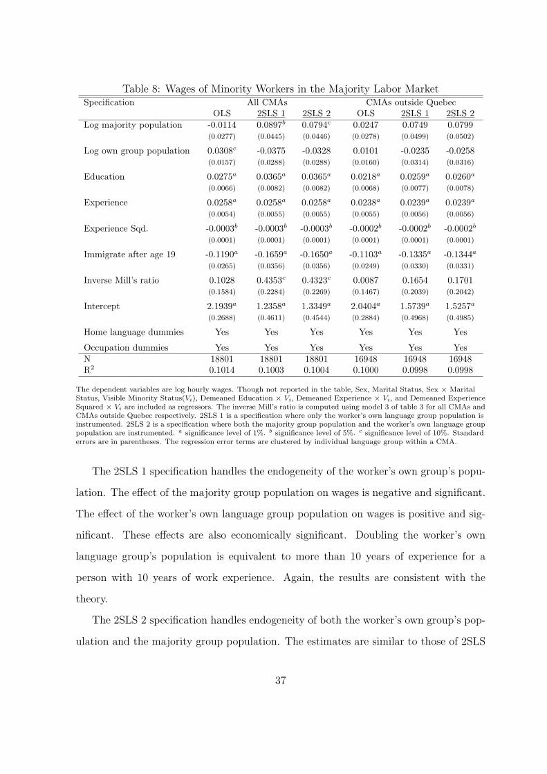
Table 8: Wages of Minority Workers in the Majority Labor MarketSpecification All CMAs CMAs outside Quebec

OLS 2SLS 1 2SLS 2 OLS 2SLS 1 2SLS 2Log majority population -0.0114 0.0897b 0.0794c 0.0247 0.0749 0.0799

(0.0277) (0.0445) (0.0446) (0.0278) (0.0499) (0.0502)

Log own group population 0.0308c -0.0375 -0.0328 0.0101 -0.0235 -0.0258(0.0157) (0.0288) (0.0288) (0.0160) (0.0314) (0.0316)

Education 0.0275a 0.0365a 0.0365a 0.0218a 0.0259a 0.0260a

(0.0066) (0.0082) (0.0082) (0.0068) (0.0077) (0.0078)

Experience 0.0258a 0.0258a 0.0258a 0.0238a 0.0239a 0.0239a

(0.0054) (0.0055) (0.0055) (0.0055) (0.0056) (0.0056)

Experience Sqd. -0.0003b -0.0003b -0.0003b -0.0002b -0.0002b -0.0002b

(0.0001) (0.0001) (0.0001) (0.0001) (0.0001) (0.0001)

Immigrate after age 19 -0.1190a -0.1659a -0.1650a -0.1103a -0.1335a -0.1344a

(0.0265) (0.0356) (0.0356) (0.0249) (0.0330) (0.0331)

Inverse Mill’s ratio 0.1028 0.4353c 0.4323c 0.0087 0.1654 0.1701(0.1584) (0.2284) (0.2269) (0.1467) (0.2039) (0.2042)

Intercept 2.1939a 1.2358a 1.3349a 2.0404a 1.5739a 1.5257a

(0.2688) (0.4611) (0.4544) (0.2884) (0.4968) (0.4985)

Home language dummies Yes Yes Yes Yes Yes Yes

Occupation dummies Yes Yes Yes Yes Yes YesN 18801 18801 18801 16948 16948 16948R2 0.1014 0.1003 0.1004 0.1000 0.0998 0.0998

The dependent variables are log hourly wages. Though not reported in the table, Sex, Marital Status, Sex × MaritalStatus, Visible Minority Status(Vi), Demeaned Education × Vi, Demeaned Experience × Vi, and Demeaned ExperienceSquared × Vi are included as regressors. The inverse Mill’s ratio is computed using model 3 of table 3 for all CMAs andCMAs outside Quebec respectively. 2SLS 1 is a specification where only the worker’s own language group population isinstrumented. 2SLS 2 is a specification where both the majority group population and the worker’s own language grouppopulation are instrumented. a significance level of 1%. b significance level of 5%. c significance level of 10%. Standarderrors are in parentheses. The regression error terms are clustered by individual language group within a CMA.

The 2SLS 1 specification handles the endogeneity of the worker’s own group’s popu-

lation. The effect of the majority group population on wages is negative and significant.

The effect of the worker’s own language group population on wages is positive and sig-

nificant. These effects are also economically significant. Doubling the worker’s own

language group’s population is equivalent to more than 10 years of experience for a

person with 10 years of work experience. Again, the results are consistent with the

theory.

The 2SLS 2 specification handles endogeneity of both the worker’s own group’s pop-

ulation and the majority group population. The estimates are similar to those of 2SLS

37

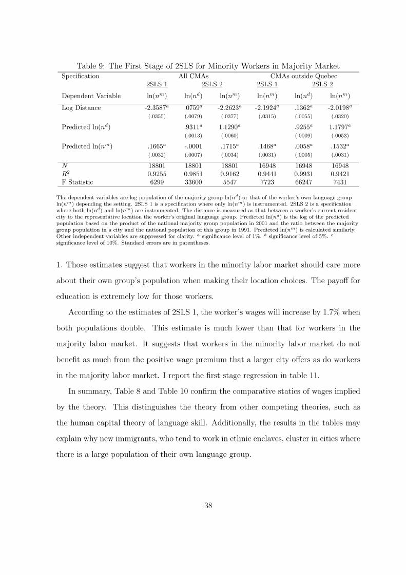
Table 9: The First Stage of 2SLS for Minority Workers in Majority MarketSpecification All CMAs CMAs outside Quebec

2SLS 1 2SLS 2 2SLS 1 2SLS 2

Dependent Variable ln(nm) ln(nd) ln(nm) ln(nm) ln(nd) ln(nm)

Log Distance -2.3587a .0759a -2.2623a -2.1924a .1362a -2.0198a

(.0355) (.0079) (.0377) (.0315) (.0055) (.0320)

Predicted ln(nd) .9311a 1.1290a .9255a 1.1797a

(.0013) (.0060) (.0009) (.0053)

Predicted ln(nm) .1665a -.0001 .1715a .1468a .0058a .1532a

(.0032) (.0007) (.0034) (.0031) (.0005) (.0031)

N 18801 18801 18801 16948 16948 16948R2 0.9255 0.9851 0.9162 0.9441 0.9931 0.9421F Statistic 6299 33600 5547 7723 66247 7431

The dependent variables are log population of the majority group ln(nd) or that of the worker’s own language groupln(nm) depending the setting. 2SLS 1 is a specification where only ln(nm) is instrumented. 2SLS 2 is a specificationwhere both ln(nd) and ln(nm) are instrumented. The distance is measured as that between a worker’s current residentcity to the representative location the worker’s original language group. Predicted ln(nd) is the log of the predictedpopulation based on the product of the national majority group population in 2001 and the ratio between the majoritygroup population in a city and the national population of this group in 1991. Predicted ln(nm) is calculated similarly.Other independent variables are suppressed for clarity. a significance level of 1%. b significance level of 5%. c

significance level of 10%. Standard errors are in parentheses.

1. Those estimates suggest that workers in the minority labor market should care more

about their own group’s population when making their location choices. The payoff for

education is extremely low for those workers.

According to the estimates of 2SLS 1, the worker’s wages will increase by 1.7% when

both populations double. This estimate is much lower than that for workers in the

majority labor market. It suggests that workers in the minority labor market do not

benefit as much from the positive wage premium that a larger city offers as do workers

in the majority labor market. I report the first stage regression in table 11.

In summary, Table 8 and Table 10 confirm the comparative statics of wages implied

by the theory. This distinguishes the theory from other competing theories, such as

the human capital theory of language skill. Additionally, the results in the tables may

explain why new immigrants, who tend to work in ethnic enclaves, cluster in cities where

there is a large population of their own language group.

38

Table 10: Wages of Minority Workers in the Minority Labor MarketSpecification All CMAs CMAs outside Quebec

OLS 2SLS 1 2SLS 2 OLS 2SLS 1 2SLS 2Log majority population -0.0432 -0.1242a -0.1206a -0.0889 -0.1472b -0.1412b

(0.0483) (0.0436) (0.0449) (0.0605) (0.0577) (0.0586)

Log own group population 0.0802b 0.1410a 0.1387a 0.1034b 0.1469a 0.1445a

(0.0317) (0.0335) (0.0342) (0.0430) (0.0455) (0.0459)

Education -0.0039 -0.0171 -0.0167 -0.008 -0.0171 -0.017(0.0134) (0.0152) (0.0153) (0.0128) (0.0161) (0.0160)

Experience 0.0129b 0.0134b 0.0134b 0.0174b 0.0175b 0.0175b

(0.0058) (0.0057) (0.0057) (0.0069) (0.0068) (0.0068)

Experience Sqd. -0.0001 -0.0001 -0.0001 -0.0002 -0.0002 -0.0002(0.0001) (0.0001) (0.0001) (0.0001) (0.0001) (0.0001)

Immigrate after age 19 0.0283 0.0857 0.0837 0.0431 0.0841 0.0828(0.0572) (0.0589) (0.0590) (0.0698) (0.0766) (0.0767)

Inverse Mill’s ratio 0.4767c 0.7524a 0.7431b 0.4382c 0.6211c 0.6166c

(0.2420) (0.2845) (0.2863) (0.2608) (0.3265) (0.3246)

Intercept 1.5876a 1.8482a 1.8304a 2.1017a 2.3011a 2.2484a

(0.5510) (0.5151) (0.5218) (0.5567) (0.5046) (0.5088)

Home language dummies Yes Yes Yes Yes Yes YesOccupation dummies Yes Yes Yes Yes Yes YesN 7136 7136 7136 6331 6331 6331R2 0.0609 0.0601 0.0601 0.0627 0.0624 0.0624

The dependent variables are log hourly wages. Though not reported in the table, Sex, Marital Status, Sex × MaritalStatus, Visible Minority Status(Vi), Demeaned Education × Vi, Demeaned Experience × Vi, and Demeaned ExperienceSquared × Vi are included as regressors. The inverse Mill’s ratio is computed using model 3 of table 3 for all CMAs andCMAs outside Quebec respectively. 2SLS 1 is a specification where only the worker’s own language group population isinstrumented. 2SLS 2 is a specification where both the majority group population and the worker’s own language grouppopulation are instrumented. a significance level of 1%. b significance level of 5%. c significance level of 10%. Standarderrors are in parentheses. The regression error terms are clustered by individual language group within a CMA.

4.3 Robustness and Discussions

4.3.1 Different Wage Measures

I chose log hourly wage as the dependent variable, to be consistent with the labor eco-

nomics literature. I also measure wages as ‘log annual wages’ or ‘raw annual wages’.

These different specifications provide essentially the same results. The tables are avail-

able upon request.

39

Table 11: The First Stage of 2SLS for Minority Workers in Minority MarketSpecification All CMAs CMAs outside Quebec

2SLS 1 2SLS 2 2SLS 1 2SLS 2

Dependent Variable ln(nm) ln(nd) ln(nm) ln(nd) ln(nd) ln(nm)

Log Distance -2.5346a -.1005a -2.5753a -2.0980a .0136c -2.0937a

(.0517) (.0133) (.0571) (.0444) (.0081) (.0447)

Predicted ln(nd) .9203a .9836a .9181a 1.061a

(.0025) (.0108) (.0016) (.0087)

Predicted ln(nm) .2442a .0008 .2631a .2156a .0049a .2178a

(.0061) (.0016) (.0067) (.0057) (.0010) (.0057)

N 7136 7136 7136 6331 6331 6331R2 0.9325 0.9796 0.9191 0.9531 0.9933 0.9525F Statistic 2651 9204 2180 3459 25348 3411

The dependent variables are log population of the majority group ln(nd) or that of the worker’s own language groupln(nm) depending the setting. 2SLS 1 is a specification where only ln(nm) is instrumented. 2SLS 2 is a specificationwhere both ln(nd) and ln(nm) are instrumented. The distance is measured as that between a worker’s current residentcity to the representative location the worker’s original language group. Predicted ln(nd) is the log of the predictedpopulation based on the product of the national majority group population in 2001 and the ratio between the majoritygroup population in a city and the national population of this group in 1991. Predicted ln(nm) is calculated similarly.Other independent variables are suppressed for clarity. a significance level of 1%. b significance level of 5%. c

significance level of 10%. Standard errors are in parentheses.

4.3.2 Bilingualism

Previously, I excluded French speaking workers outside Quebec and English speaking

workers in Quebec from the analysis. In this section, I restrict the sample to English

speaking or French speaking workers only. I explore whether the bilingual policy in

Canada has an effect on those workers’ wages. Throughout the paper, “bilingual” means

a person can communicate in both English and French.

Table 12 shows the determinants of the labor market choices of English or French

speaking workers. The first subsample includes workers who speak French at home and

live outside Quebec. They choose their work language: French versus English. The

second subsample includes workers who speak English at home and live in Quebec.

They also choose their work language: English versus French.

The estimates are not as intuitive as those in table 3. For example, a more educated

French-speaking worker is less likely to speak English at work. Outside Quebec, there

are a lot of government jobs that require French language skills. To the extent that gov-

40

Table 12: Labor Market Choices of Official Language SpeakersOutside Quebec In Quebec

Model 1 Model 2 Model 1 Model 2Education -0.0511a -0.0664a -0.0484a -0.0501a

(0.0077) (0.0080) (0.0054) (0.0055)

Age -0.0060a -0.0063a -0.0038a -0.0040a

(0.0016) (0.0016) (0.0010) (0.0010)

Sex (Female=1) -0.2563a -0.2531a 0.0154 0.0192(0.0407) (0.0412) (0.0269) (0.0270)

Immigrate after age 19 0.0981 0.0098 -0.1866a -0.1557a

(0.0732) (0.0745) (0.0472) (0.0474)

Log own group population -0.3441a -0.2931a

(0.0317) (0.0515)

Log majority population 0.3091a 0.3458a

(0.0273) (0.1283)

Intercept 0.9354a 0.4311 -0.0723 -0.9901(0.1282) (0.3081) (0.0860) (1.1218)

N 3901 3901 11894 11894Pseudo R2 0.0183 0.0479 0.011 0.0216

The dependent variable is the worker’s language at work. It equals 1 if it is English (or Frenchin Quebec), 0 otherwise. Minority workers are those whose home languages are neither Englishnor French. a significance level of 1%. b significance level of 5%. c significance level of 10%.Standard errors are in parentheses.

ernment jobs require higher education, a positive correlation between speaking French

at work and education may exist. An English speaking worker in Quebec is also less

likely to speak French at work if she is more educated. The effects of populations are

nonetheless compatible with the language theory.

Table 13 reports the Within-labor-market Wage Gap estimates. The two groups to

be compared in provinces outside Quebec are English-speaking workers (majority) and

French-speaking workers (minority) who speak English at work. The two comparison

groups in Quebec are French-speaking workers (majority) and English-speaking workers

(minority) who speak French at work. The estimates are mostly insignificant. The

differences in the marginal effects of education and experience are also insignificant.

There are two explanations for the results. First, the language barrier between the

English-speaking population and French-speaking population is small enough to have

no effect on wages. Secondly, bilingual workers are paid more to compensate for their

41

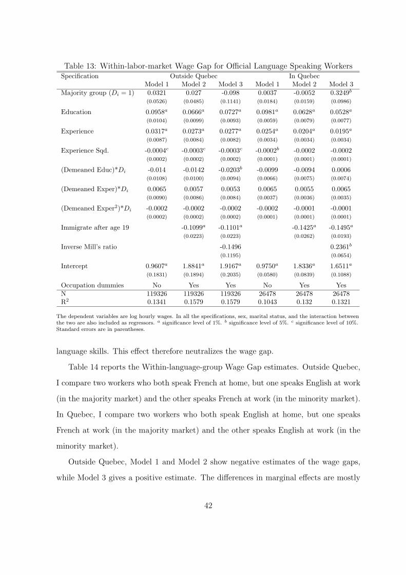
Table 13: Within-labor-market Wage Gap for Official Language Speaking WorkersSpecification Outside Quebec In Quebec

Model 1 Model 2 Model 3 Model 1 Model 2 Model 3Majority group (Di = 1) 0.0321 0.027 -0.098 0.0037 -0.0052 0.3249b

(0.0526) (0.0485) (0.1141) (0.0184) (0.0159) (0.0986)

Education 0.0958a 0.0666a 0.0727a 0.0981a 0.0628a 0.0528a

(0.0104) (0.0099) (0.0093) (0.0059) (0.0079) (0.0077)

Experience 0.0317a 0.0273a 0.0277a 0.0254a 0.0204a 0.0195a

(0.0087) (0.0084) (0.0082) (0.0034) (0.0034) (0.0034)

Experience Sqd. -0.0004c -0.0003c -0.0003c -0.0002b -0.0002 -0.0002(0.0002) (0.0002) (0.0002) (0.0001) (0.0001) (0.0001)

(Demeaned Educ)*Di -0.014 -0.0142 -0.0203b -0.0099 -0.0094 0.0006(0.0108) (0.0100) (0.0094) (0.0066) (0.0075) (0.0074)

(Demeaned Exper)*Di 0.0065 0.0057 0.0053 0.0065 0.0055 0.0065(0.0090) (0.0086) (0.0084) (0.0037) (0.0036) (0.0035)

(Demeaned Exper2)*Di -0.0002 -0.0002 -0.0002 -0.0002 -0.0001 -0.0001(0.0002) (0.0002) (0.0002) (0.0001) (0.0001) (0.0001)

Immigrate after age 19 -0.1099a -0.1101a -0.1425a -0.1495a

(0.0223) (0.0223) (0.0262) (0.0193)

Inverse Mill’s ratio -0.1496 0.2361b

(0.1195) (0.0654)

Intercept 0.9607a 1.8841a 1.9167a 0.9750a 1.8336a 1.6511a

(0.1831) (0.1894) (0.2035) (0.0580) (0.0839) (0.1088)

Occupation dummies No Yes Yes No Yes YesN 119326 119326 119326 26478 26478 26478R2 0.1341 0.1579 0.1579 0.1043 0.132 0.1321

The dependent variables are log hourly wages. In all the specifications, sex, marital status, and the interaction betweenthe two are also included as regressors. a significance level of 1%. b significance level of 5%. c significance level of 10%.Standard errors are in parentheses.

language skills. This effect therefore neutralizes the wage gap.

Table 14 reports the Within-language-group Wage Gap estimates. Outside Quebec,

I compare two workers who both speak French at home, but one speaks English at work

(in the majority market) and the other speaks French at work (in the minority market).

In Quebec, I compare two workers who both speak English at home, but one speaks

French at work (in the majority market) and the other speaks English at work (in the

minority market).

Outside Quebec, Model 1 and Model 2 show negative estimates of the wage gaps,

while Model 3 gives a positive estimate. The differences in marginal effects are mostly

42

Table 14: Within-language-group Wage Gap for Official Language Speaking WorkersSpecification Outside Quebec In Quebec

Model 1 Model 2 Model 3 Model 1 Model 2 Model 3Majority market (Li = 1) -0.0769b -0.0578 0.3613c -0.0098 0.0072 -0.3959

(0.0337) (0.0347) (0.1915) (0.0119) (0.0127) (0.1814)

Education 0.0732a 0.0555a 0.0631a 0.0875a 0.0600a 0.0578a

(0.0099) (0.0101) (0.0117) (0.0042) (0.0047) (0.0048)

Experience 0.0402a 0.0363a 0.0375a 0.0371a 0.0334a 0.0332a

(0.0077) (0.0072) (0.0074) (0.0008) (0.0007) (0.0007)

Experience Sqd. -0.0006a -0.0005a -0.0005a -0.0005a -0.0005a -0.0005a

(0.0002) (0.0002) (0.0002) (0.0000) (0.0000) (0.0000)

(Demeaned Educ)*Li 0.0231 0.0204 0.0258b 0.0106 0.008 -0.0005(0.0136) (0.0127) (0.0098) (0.0102) (0.0105) (0.0058)

(Demeaned Exper)*Li -0.007 -0.0066 -0.0072 -0.0120c -0.0121c -0.0130c

(0.0088) (0.0089) (0.0093) (0.0037) (0.0040) (0.0042)

(Demeaned Exper2)*Li 0.0002 0.0002 0.0002 0.0003 0.0003 0.0003(0.0002) (0.0002) (0.0002) (0.0001) (0.0001) (0.0001)

Immigrate after age 19 -0.2642b -0.2804a -0.1931a -0.2053a

(0.0914) (0.0895) (0.0130) (0.0138)

Correction for Li = 1 -0.2944c 0.255(0.1501) (0.1166)

Correction for Li = 0 0.2402b -0.1147(0.1066) (0.1258)

Intercept 1.3174a 1.8605a 1.5322a 1.0563a 1.8244a 1.8944a

(0.2228) (0.1576) (0.2213) (0.0601) (0.1159) (0.1158)

Occupation dummies No Yes Yes No Yes YesN 2959 2959 2959 8912 8912 8912R2 0.1212 0.144 0.1457 0.1082 0.1335 0.1338

The dependent variables are log hourly wages. In all the specifications, sex, marital status, and the interaction betweenthe two are also included as regressors.a significance level of 1%. b significance level of 5%. c significance level of 10%.Standard errors are in parentheses.

insignificant. In Quebec, the estimated Within-language-group Wage Ggaps are insignif-

icant. The differences in marginal effects are also insignificant.

Table 13 and table 14 show that official language speakers are paid similarly no

matter which language group they belong to or which work language they choose. This

is certainly different from what I found before. The language theory fails to explain this

pattern. There is something else affecting those workers’ earnings. Is it the bilingual

policy? I have to leave the answer to this question to future research.

43

5 Conclusion

This paper presents a simple model of labor market segmentation in which language

plays a significant role. An urban labor market has several segments, in which the

languages of business communications are different. The majority labor market has a

larger number of workers and firms, so it offers higher matching quality and hence higher

wages.

In equilibrium, there are two types of wage gaps. The Within-labor-market Wage

Gap exists between a majority worker and a minority worker who both work in the ma-

jority labor market. The Within-language-group Wage Gap exists between two minority

workers who work in different labor markets.

Another key implication is the relationship between workers’ wages and language

group populations. Wages in the majority labor market increase with the majority

population due to the market thickness effect. On the other hand, wages in the minority

labor market decrease with the majority population, because minority workers leave the

minority labor market and enter the majority labor market as the majority labor market

becomes thicker.

Wages in the minority labor market increase with the minority population, again

due to the market thickness effect. However, wages in the majority labor market may

increase or decrease with the minority population. The latter is because the number

of minority workers in the majority labor market can either increase or decrease as the

minority population increases.

I tested those predictions using 2001 Canadian Census Public Use Micro Data. The

reported work language in the data allowed me to identify a worker’s labor market. I

confirmed the existence of both types of wage gaps. The marginal effects of population

measures on wages were consistent with the theory. These results are unique to the

language theory of labor market segmentation, and they differentiate the theory from

other competing theories.

44

Interestingly, bilingualism policy seems to increase the wages of French and English

speaking workers. A more rigorous research has to be carried out to determine whether

this is true. Moreover, further research is needed to show how this policy affects workers

in other language groups and especially their location choices.

A lot of testable implications of the theory have been left out due to data limitations.

The theory also provides a framework with which to understand the workings of the

urban labor market. It may aid policy makers in framing or implementing immigration

and language policies in the future.

A Derivations

A.1 The Derivation of Matching Quality

We begin with the matching quality of majority group workers. First, note that |x − y| is a

uniform random variable over the interval [y, y+1/2] on the unit circle. Its probability density

is 2. Therefore, the probability that a worker with characteristic x belongs to the market area

of a firm with address y is

Pr(|x− y| < 1/2ml) =∫ 1/2ml

02dµ = 1/ml. (20)

The event that a worker x is employed by firm y is a Bernoulli random variable. The number

of majority workers employed by the firm Ωdl (y) therefore follows a binomial distribution with

parameters ndl and 1/ml. The expected employment is hence E[Ωd

l (y)] = ndl

ml.

The expected distance on the unit circle between a firm’s employee and the firm can be

expressed as E[|x− y| : x ∈ (y − 12ml

, y + 12ml

)]. The probability density distribution function

of |x− y| conditional on the worker belongs to the firm’s market area is

f [|x− y| : x ∈ (y − 12ml

, y +1

2ml)] =

2Pr[x∈(y− 1

2ml,y+ 1

2ml)]

if x ∈ (y − 12ml

, y + 12ml

)

0 if x < y − 12ml

or x > y + 12ml

The denominator is 1/ml (equation (20)) in the first case. Therefore, the conditional expec-

tation of |x− y| equals

E[|x− y| : x ∈ (y − 12ml

, y +1

2ml)] =

∫ 1/2ml

02mlµdµ = 1/4ml. (21)

45

The expected distance decreases as ml increases. The expected distance between a minority

worker and the firm can be derived analogously. It is also 1/4ml.

A.2 Proof of Lemma 2

First, I derive the expected profit in the majority labor market E(πld). We know that πld =

qld − κld . The combination of equation (4), (5), and (6) gives

πld

(y, Ωd

ld(y),Ωm

ld(y)

)= 1

2

∑i∈Ωd

ld(y)

(αd + ξi − βd

ld|xi − y|

)

+∑

i∈Ωmld

(y)

(αm + ξi − βm

ld|xi − y|

)− Cld .

The expected revenue earned from the set of majority group workers Ωdld

can be expressed as

E[∑

i∈Ωdld

(y)(αd + ξi − βd

ld|xi − y|)]

= E[∑Ωd

ld(y)

i=1 (αd + ξi − βdld|xi − y|) : i ∈ Ωd

ld(y)]

= E[∑Ωd

ld(y)

i=1 (αd + ξi − βdld|xi − y|) : |xi − y| < 1

2mld]

= E[∑Ωd

ld(y)

i=1 (αd + ξi)]− E[∑Ωd

ld(y)

i=1 βdld|xi − y| : |xi − y| < 1

2mld]

= E[Ωdld

(y)]αd − E[Ωdld

(y)]E[|xi − y| : |xi − y| < 12mld

]βdld

= (nd/mld)(αd − βd

ld/(4mld)).

The first and second equalities are re-expressions of the expected revenue. The third equality

uses the assumption that xi is independent of both ξi and ψi, which implies the independence

between Ωdld

and xi, and also ξi and xi. The next equality employs the independence between

Ωdld

and xi and assumption about ξi. The last equality employs the results in section A.1.

The expected revenue earned from the set of minority workers Ωmld

is complicated.

E[∑

i∈Ωmld

(y)(αm + ξi − βm

ld|xi − y|)]

= E[∑Ωm

ld(y)

i=1 (αm + ξi − βmld|xi − y|) : i ∈ Ωm

ld(y)]

= E[∑Ωm

ld(y)

i=1 (αm + ξi − βmld|xi − y|) : ψi < µ, |xi − y| < 1

2mld]

= E[∑Ωm

ld(y)

i=1 (αm + ξi) : ψi < µ]− E[∑Ωm

ld(y)

i=1 βmld|xi − y| : ψi < µ, |xi − y| < 1

2mld]

= E[Ωmld

(y)]αm + E[Ωmld

(y)]E[ξi : ψi < µ]− E[Ωmld

(y)]E[|xi − y| : |xi − y| < 12mld

]βmld

= (nm · Φ(µ/σ)/mld)(αm − ρs φ(µ/σ)

Φ(µ/σ) − βmld

/(4mld)).

The difference lies in the second equality, where I add ψi < µ where µ = (βmlm

/8mlm) −(βm

ld/8mld) − θm

ld. Only those workers whose ψ’s satisfy the inequality enter the majority

labor market. The third equality again uses the independence of xi with both ψi and ξi.

46

The next equality uses the independence between Ωmld

and ψi. Strictly speaking, this is only

approximately true as nm becomes large enough.20 The last equality uses joint normality of

ξi and ψi, and φ(µ/σ)Φ(µ/σ) is the inverse Mill’s ratio. The last equality uses results in section A.1

as well.

Substituting the above two terms into the expected profit expression gives the results of

the lemma. Analogously, I can derive the expected profit in the minority labor market.

A.3 Proof of Proposition 1

Under assumptions made in Proposition 1, the two equilibrium conditions are

E(πld) =nd

2mld

(αd − βdld

4mld

) +nm · Φ(µ/σ)

2mld

[αm − βmld

4mld

]− Cld = 0, and

E(πlm) =nm · (1− Φ(µ/σ))

2mlm

[αm − βmlm

4mlm

]− Clm = 0.

Note µ = (βmlm

/8mlm) − (βmld

/8mld) − θmld

. The selection correction terms disappear because

ρ = 0. The Jacobian J with respect to mld and mlm of the two equations is

∂E[πld]

∂mld

∂E[πld]

∂mlm

∂E[πlm ]∂mld

∂E[πlm ]∂mld

=

nd ∂F1∂mld

+ nm ∂Φ∂mld

F2 + nmΦ ∂F2∂mld

nm ∂Φ∂mlm

F2

−nmF3∂Φ

∂mld−nmF3

∂Φ∂mlm

+ nm(1− Φ) ∂F3∂mlm

.

Here F1 = 12mld

(αd − βdld

4mld), F2 = 1

2mld(αm − βm

ld4mld

), and F3 = 12mlm

(αm − βmlm

4mlm). It is

straightforward to verify that∂E[πld

]

∂mlm< 0 and ∂E[πlm ]

∂mld< 0. Because J is assumed to be

negative definite,∂E[πld

]

∂mld< 0 and ∂E[πlm ]

∂mld< 0.

E(πld) and E(πlm) are continuously differentiable with respect to mld and mlm . We assume

that J is negative definite, so |J | > 0. The comparative statics is hence well-defined due to

the Implicit Function Theorem. Take total differential of the equation system, we get

∂E[πld]

∂mlddmld +

∂E[πld]

∂mlmdmlm = −

(∂E[πld

]

∂nlddnld + · · ·+ ∂E[πld

]

∂σ dσ)

∂E[πlm ]∂mld

dmld + ∂E[πlm ]∂mlm

dmlm = −(

∂E[πlm ]∂nld

dnld + · · ·+ ∂E[πlm ]∂σ dσ

),

20Because ψi’s are independent across workers, the random variable nmld

is approximately independentof a particular ψi as nm increases.

47

where I omit several exogenous variables to simplify the expression. Let all the differentials

be zeros except dnld and then divide both sides of the equation system by dnld . I get

∂E[πld]

∂mld

∂E[πld]

∂mlm

∂E[πlm ]∂mld

∂E[πlm ]∂mlm

∂mld∂nld

∂mlm∂nld

=

−∂E[πld

]

∂nld

−∂E[πlm ]∂nld

By Cramer’s rule, the solution of this system can be written

∂mld

∂nld

=|J1||J | , and

∂mlm

∂nld

=|J2||J | , (22)

where |.| denotes the determinant of the matrix, J is the Jacobian of the equation system,

and Ji is the new matrix formed by substituting the right-hand side column vector to the ith

column of the Jacobian.

It is easy to calculate that −∂E[πld]

∂nld= −F1 and −∂E[πlm ]

∂nld= 0. We also know that all the

terms in the Jacobian are negative. Using equation (22), it is straightforward to show that∂mld∂nld

> 0 and ∂mlm∂nld

< 0. The comparative statics with respect to other exogenous variables

αd, Clm , βmlm

, θmld

, Cld , βdld

, βmld

, nm, αm, and σ can be derived following similar steps.

B A Generalized Model of Labor Market Segmen-

tation

This section contains a generalization of the basic model to multiple language groups and

multiple labor markets. I continue to use superscript k = 1, ..., K to represent a worker’s

language group, where “1” denotes the majority group and K is the number of language

groups. All other groups are minorities. The population of a language group is denoted nk.

I use subscript l = 1, ..., L to index the labor market, where “1” represents the majority

labor market and L is the number of labor markets. The number of workers who belong to

language group k and work in labor market l is denoted nkl . Note that K = L must hold.

Assumption 2. (1) Majority group workers work only in the majority market;

(2) Minority workers can choose only between the majority labor market and their own lan-

guage groups’ labor market.

(3) The conditions in Assumption 1 hold.

48

Under Assumption 2, the choice for a minority worker of language group k is between labor

market l = 1 and labor market l = k. The expected net wage can be expressed as

E(Uk

l,i

)=

12 [αk + ξi − βk

14m1

]− θk1 − ψi if l = 1, and k = 2, ..., K

12 [αk + ξi − βk

k4mk

] if l = k, and k = 2, ..., K

. (23)

The minority worker chooses the majority labor market if and only if (βkk/8mk)− (βk

1/8m1)−θk1 − ψi > 0.

The number of minority workers of language group k ≥ 2 in the majority labor market nklm

is a binomial random variable. Its expectation is nkΦ(µ/σ), where µ = (βkk/8mk)−(βk

1/8m1)−θk1 and σ is the standard deviation of ψi. Similarly, the expected number of workers belonging

to group k in language group k’s labor market is nk(1 − Φ(µ/σ)). Notice the similarity to

Lemma 1.

Lemma 3. Under Assumption 2, the following statements hold. In the majority group’s labor

market, the expected profit of a firm that has an address y on the unit circle is

E(π1) =n1

2m1(α1 − β1

1

4m1) +

K∑

k=2

nk · Φ(µ/σ)2m1

[αk − ρsφ(µ/σ)Φ(µ/σ)

− βk1

4m1]− C1. (24)

In the minority group’s labor market, the firm’s expected profit is

E(πk) =nk · (1− Φ(µ/σ))

2mk[αk + ρs

φ(µ/σ)1− Φ(µ/σ)

− βkk

4mk]− Ck. (25)

Note µ = (βkk/8mk)− (βk

1/8m1)− θk1 .

Proof. The proof is analogous to that of Lemma 2 and is omitted.

The result is analogous to that of Lemma 2. Since minority workers in the majority labor

market belong to several language groups, the firm’s revenue is composed of contributions from

minority workers of K − 1 groups. Also notice that equation (25) actually represents K − 1

equations.

The zero-profits conditions then characterize the equilibrium number of firms ml, l =

49

1, ..., L(K). The Jacobian J associated with the zero-profits conditions is

J =

∂E[π1]∂m1

∂E[π1]∂m2

∂E[π1]∂m3

· · · ∂E[π1]∂mK

∂E[π2]∂m1

∂E[π2]∂m2

0 · · · 0∂E[π3]∂m1

0 ∂E[π3]∂m3

· · · 0...

......

. . ....

∂E[πK ]∂m1

0 0 · · · ∂E[πK ]∂mK

.

Note that except on the diagonal, the first column, and the first row, all other elements are

zeros.

Proposition 4. If (1) Assumption 2 holds, (2) the model parameters are such that there is

at least one equilibrium (m1, ..., mL) such that ml > 0 for all l = 1, ..., L, (3) ρ = 0, and

(4) Evaluated at the equilibrium (m1, ..., mL), J is negative definite, the following comparative

statics hold at the equilibrium (m1, ..., mL) for k, k′ = 2, ..., K and k 6= k′.

1. As (a) n1, α1, Ck, or βkk increases, or (b) θk

1 , C1, β11 , or βk

1 decreases, m1 increases.

The comparative statics of m1 with respect to nk, αk, and σ are ambiguous.

2. As (a) n1, α1, Ck, or βkk increases, or (b) θk

1 , C1, β11 , or βk

1 decreases, mk decreases.

The comparative statics of mk with respect to nk, αk, and σ are ambiguous.

3. As (a) Ck or βkk increases, or (b) θk

1 or βk1 decreases, mk′ decreases. The comparative

statics with respect to nk, αk, and σ are ambiguous.

Proof. It is straightforward to verify the continuous differentiability of the zero-profits equa-

tions. It is also true that |J | 6= 0 at the equilibrium because of the assumption. Therefore, the

implicit function theorem holds and the equation system defines a set of implicit functions for

ml where l = 1, 2, · · · ,K. Following similar steps in the proof of Proposition 1, I get

∂E[π1]∂m1

∂E[π1]∂m2

· · · ∂E[π1]∂mK

∂E[π2]∂m1

∂E[π2]∂m2

· · · 0...

.... . .

...∂E[πK ]

∂m10 · · · ∂E[πK ]

∂mK

∂m1∂φ

∂m2∂φ

...∂mK∂φ

=

−∂E[π1]∂φ

−∂E[π2]∂φ

...−∂E[πK ]

∂φ

,

where φ represents any exogenous variable in the model. Using Cramer’s rule, the derivative

of mk with respect to φ can be written

∂mk

∂φ=|Jk||J | , k = 1, 2, ..., K (26)

50

where Jk is the new matrix formed by substituting the right-hand side column vector to

the kth column of the Jacobian J . Note also that ∂E[π1]∂mk

= nk ∂Φ∂mk

αk−(βk1 /4m1)

2m1< 0 and

∂E[πk]∂m1

= −nk ∂Φ∂m1

αk−(βkk/4mk)

2mk< 0 for all k = 2, ..., K.

I pick the comparative static of m1, mk, and mk′ with respect to βk1 as an example, where

k′ 6= k and k, k′ = 2, ..., K. It is easy to verify that −∂E[π1]

∂βk1

> 0, −∂E[πk]

∂βk1

< 0, and −∂E[πk′ ]∂βk

1= 0.

First, I derive the result for m1. I can calculate |J1| as

|J1| = (−∂E[π1]

∂βk1

∂E[πk]∂mk

− −∂E[πk]

∂βk1

∂E[π1]∂mk

)∏

l 6=1,k∂E[πl]∂ml

.

Using assumptions that ∂E[πk]∂mk

< 0 and the results that −∂E[π1]

∂βk1

> 0, −∂E[πk]

∂βk1

< 0, and∂E[π1]∂mk

< 0, we get that sign(|J1|) = sign((−1)K−1). We know that sign(|J |) = sign((−1)K),

so ∂m1

∂βk1

< 0.

Next, I derive the result for mk′ , where k′ 6= k. I calculate |Jk′ | as

|Jk′ | = −∂E[πk]∂m1

(−∂E[π1]

∂βk1

∂E[πk]∂mk

− −∂E[πk]

∂βk1

∂E[π1]∂mk

)∏

l 6=1,k′,k∂E[πl]∂ml

.

Using similar argument as in the first case, we get sign(|Jk′ |) = sign((−1)K−2), so ∂mk′∂βk

1> 0.

Lastly, I derive the result for mk. This case is more complicated. The determinant of Jk is

|Jk| = −∂E[πk]

∂βk1

(∏

l 6=k∂E[πl]∂ml

−∑l 6=1,k[

∂E[πl]∂m1

∂E[π1]∂ml

∏j 6=1,k,l

∂E[πj ]∂mj

])

− −∂E[π1]

∂βk1

∂E[πk]∂m1

∏l 6=1,k

∂E[πl]∂ml

.

We can verify that∏

l 6=k∂E[πl]∂ml

− ∑l 6=1,k[

∂E[πl]∂m1

∂E[π1]∂ml

∏j 6=1,k,l

∂E[πj ]∂mj

] is the determinant of a

submatrix of J . This submatrix is obtained by removing the kth row and kth column of

J . Because J is negative definite, the sign of the determinant of this submatrix is (−1)K−1.

It is the feedback effect from other minority markets to minority market k. Using previous

assumptions and results, we get that sign(|Jk|) = sign((−1)K). As a result, ∂mk

∂βk1

> 0. Though

tedious, it is straightforward to get all the comparative statics contained in the proposition.

Some results are familiar. For example, as majority population increases, the number of

firms in the majority labor market also increases, and the number of firms in any minority

labor market decreases.

However, some results require more delicate thought. Take the comparative statics with

respect to the language learning cost θk1 as an example. It is clear that the number of majority

51

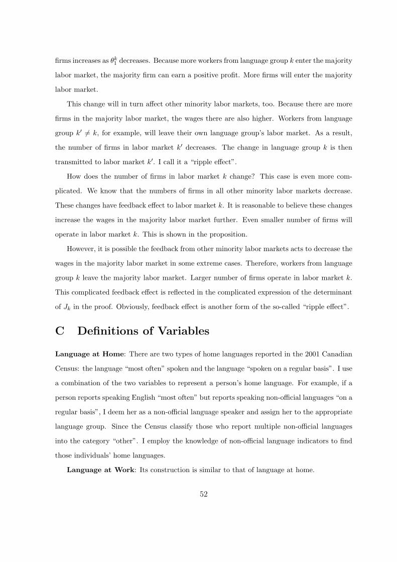
firms increases as θk1 decreases. Because more workers from language group k enter the majority

labor market, the majority firm can earn a positive profit. More firms will enter the majority

labor market.

This change will in turn affect other minority labor markets, too. Because there are more

firms in the majority labor market, the wages there are also higher. Workers from language

group k′ 6= k, for example, will leave their own language group’s labor market. As a result,

the number of firms in labor market k′ decreases. The change in language group k is then

transmitted to labor market k′. I call it a “ripple effect”.

How does the number of firms in labor market k change? This case is even more com-

plicated. We know that the numbers of firms in all other minority labor markets decrease.

These changes have feedback effect to labor market k. It is reasonable to believe these changes

increase the wages in the majority labor market further. Even smaller number of firms will

operate in labor market k. This is shown in the proposition.

However, it is possible the feedback from other minority labor markets acts to decrease the

wages in the majority labor market in some extreme cases. Therefore, workers from language

group k leave the majority labor market. Larger number of firms operate in labor market k.

This complicated feedback effect is reflected in the complicated expression of the determinant

of Jk in the proof. Obviously, feedback effect is another form of the so-called “ripple effect”.

C Definitions of Variables

Language at Home: There are two types of home languages reported in the 2001 Canadian

Census: the language “most often” spoken and the language “spoken on a regular basis”. I use

a combination of the two variables to represent a person’s home language. For example, if a

person reports speaking English “most often” but reports speaking non-official languages “on a

regular basis”, I deem her as a non-official language speaker and assign her to the appropriate

language group. Since the Census classify those who report multiple non-official languages

into the category “other”. I employ the knowledge of non-official language indicators to find

those individuals’ home languages.

Language at Work: Its construction is similar to that of language at home.

52

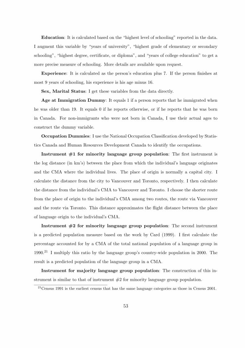
Education: It is calculated based on the “highest level of schooling” reported in the data.

I augment this variable by “years of university”, “highest grade of elementary or secondary

schooling”, “highest degree, certificate, or diploma”, and “years of college education” to get a

more precise measure of schooling. More details are available upon request.

Experience: It is calculated as the person’s education plus 7. If the person finishes at

most 9 years of schooling, his experience is his age minus 16.

Sex, Marital Status: I get these variables from the data directly.

Age at Immigration Dummy: It equals 1 if a person reports that he immigrated when

he was older than 19. It equals 0 if he reports otherwise, or if he reports that he was born

in Canada. For non-immigrants who were not born in Canada, I use their actual ages to

construct the dummy variable.

Occupation Dummies: I use the National Occupation Classification developed by Statis-

tics Canada and Human Resources Development Canada to identify the occupations.

Instrument #1 for minority language group population: The first instrument is

the log distance (in km’s) between the place from which the individual’s language originates

and the CMA where the individual lives. The place of origin is normally a capital city. I

calculate the distance from the city to Vancouver and Toronto, respectively. I then calculate

the distance from the individual’s CMA to Vancouver and Toronto. I choose the shorter route

from the place of origin to the individual’s CMA among two routes, the route via Vancouver

and the route via Toronto. This distance approximates the flight distance between the place

of language origin to the individual’s CMA.

Instrument #2 for minority language group population: The second instrument

is a predicted population measure based on the work by Card (1999). I first calculate the

percentage accounted for by a CMA of the total national population of a language group in

1990.21 I multiply this ratio by the language group’s country-wide population in 2000. The

result is a predicted population of the language group in a CMA.

Instrument for majority language group population: The construction of this in-

strument is similar to that of instrument #2 for minority language group population.

21Census 1991 is the earliest census that has the same language categories as those in Census 2001.

53

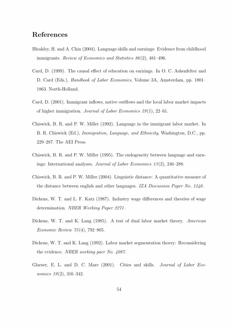
References

Bleakley, H. and A. Chin (2004). Language skills and earnings: Evidence from childhood

immigrants. Review of Economics and Statistics 86 (2), 481–496.

Card, D. (1999). The causal effect of education on earnings. In O. C. Ashenfelter and

D. Card (Eds.), Handbook of Labor Economics, Volume 3A, Amsterdam, pp. 1801–

1863. North-Holland.

Card, D. (2001). Immigrant inflows, native outflows and the local labor market impacts

of higher immigration. Journal of Labor Economics 19 (1), 22–61.

Chiswick, B. R. and P. W. Miller (1992). Language in the immigrant labor market. In

B. R. Chiswick (Ed.), Immigration, Language, and Ethnicity, Washington, D.C., pp.

229–287. The AEI Press.

Chiswick, B. R. and P. W. Miller (1995). The endogeneity between language and earn-

ings: International analyses. Journal of Labor Economics 13 (2), 246–288.

Chiswick, B. R. and P. W. Miller (2004). Linguistic distance: A quantitative measure of

the distance between english and other languages. IZA Discussion Paper No. 1246 .

Dickens, W. T. and L. F. Katz (1987). Industry wage differences and theories of wage

determination. NBER Working Paper 2271 .

Dickens, W. T. and K. Lang (1985). A test of dual labor market theory. American

Economic Review 75 (4), 792–805.

Dickens, W. T. and K. Lang (1992). Labor market segmentation thoery: Reconsidering

the evidence. NBER working paer No. 4087 .

Glaeser, E. L. and D. C. Mare (2001). Cities and skills. Journal of Labor Eco-

nomics 19 (2), 316–342.

54

Helsley, R. W. and W. C. Strange (1990). Matching and agglomeration economies in a

system of cities. Regional Science and Urban Economics 20 (2), 189–212.

Lang, K. (1986). A language theory of discrimination. Quarterly Journal of Eco-

nomics 101 (2), 363–382.

Lee, L. (1982). Some approaches to the correction of selectivity bias. Review of Economic

Studies 49 (3), 355–372.

Sutton, J. (1986). Non-cooperative bargaining theory: An introduction. Review of

Economic Studies 53 (5), 709–724.

Wardhaugh, R. (2005). An Introduction to Sociolinguistics (5 ed.). Blackwell Publishing

Limited.

Wooldridge, J. M. (2002). Econometric Analysis of Cross Section and Panel Data.

Cambridge, MA: MIT Press.

55