Lane-Exchanging Driving Strategy for AutonomousVehicle via Trajectory Prediction and ModelPredictive ControlYIMIN CHEN 

Northwestern Polytechnical UniversityHuilong Yu  ( huilong.yu@uwaterloo.ca )

University of WaterlooJinwei Zhang 

University of WaterlooDonpu Cao 

University of Waterloo

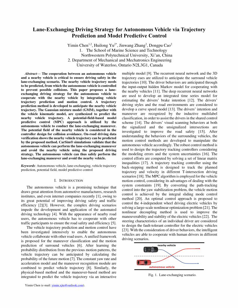
Original Article

Keywords: Autonomous vehicle, lane-exchanging, vehicle trajectory prediction, potential �eld, modelpredictive control

Posted Date: December 10th, 2020

DOI: https://doi.org/10.21203/rs.3.rs-122422/v1

License: This work is licensed under a Creative Commons Attribution 4.0 International License.  Read Full License

Abstract— The cooperation between an autonomous vehicle

and a nearby vehicle is critical to ensure driving safety in the

lane-exchanging scenario. The nearby vehicle trajectory needs

to be predicted, from which the autonomous vehicle is controlled

to prevent possible collisions. This paper proposes a lane-

exchanging driving strategy for the autonomous vehicle to

cooperate with the nearby vehicle by integrating vehicle

trajectory prediction and motion control. A trajectory

prediction method is developed to anticipate the nearby vehicle

trajectory. The Gaussian mixture model (GMM), together with

the vehicle kinematic model, are synthesized to predict the

nearby vehicle trajectory. A potential-field-based model

predictive control (MPC) approach is utilized by the

autonomous vehicle to conduct the lane-exchanging maneuver.

The potential field of the nearby vehicle is considered in the

controller design for collision avoidance. On-road driving data

verification shows the nearby vehicle trajectory can be predicted

by the proposed method. CarSim® simulations validate that the

autonomous vehicle can perform the lane-exchanging maneuver

and avoid the nearby vehicle using the proposed driving

strategy. The autonomous vehicle can thus safely perform the

lane-exchanging maneuver and avoid the nearby vehicle.

Keywords: Autonomous vehicle, lane-exchanging, vehicle trajectory prediction, potential field, model predictive control

I. INTRODUCTION

The autonomous vehicle is a promising technique that draws great attention from automotive manufactures, research institutes, and even internet companies recently [1], owing to its great potential of improving driving safety and traffic efficiency [2][3]. However, the complex driving scenarios impede the development and application of the automated driving technology [4]. With the appearance of nearby road users, the autonomous vehicle has to cooperate with other traffic participants to ensure the road safety and efficiency [5].

The vehicle trajectory prediction and motion control have been investigated intensively to enable the autonomous vehicle collaborate with other road users. A unified framework is proposed for the maneuver classification and the motion prediction of surround vehicles [6]. After learning the probability distribution from the previous motion patterns, the vehicle trajectory can be anticipated by calculating the probability of the future motion [7]. The constant yaw rate and acceleration model and the maneuver recognition module are combined to predict vehicle trajectory [8]. Similarly, the physical-based method and the maneuver-based method are integrated to predict the vehicle trajectory via an interactive

Yimin Chen (e-mail: yimin.xjtu@outlook.com).

multiple model [9]. The recurrent neural network and the 3D trajectory cues are utilized to anticipate the surround vehicle trajectories [10]. The driver behaviors are anticipated through the input-output hidden Markov model for cooperating with the nearby vehicles [11]. The deep recurrent neural networks are used to develop an integrated time series model for estimating the drivers’ brake intention [12]. The drivers’ driving styles and the road environments are considered to develop a curve speed model [13]. The drivers’ intention and maneuver are recognized by the inductive multilabel classification, in order to assist the drivers in the shared control scheme [14]. The drivers’ visual scanning behaviors at both the signalized and the unsignalized intersections are investigated to improve the road safety [15]. After understanding the behaviors of the surrounding vehicles, the motion control methods are developed to manipulate the autonomous vehicle accordingly. The robust control method is used to design the trajectory tracking controllers considering the modeling errors and the system uncertainties [16]. The control efforts are computed by solving a set of linear matrix inequalities [17]. A trajectory tracking controller using the back-stepping method is designed to track the planned trajectory and velocity in different T-intersection driving scenarios [18]. The MPC algorithm is employed for the vehicle motion control, considering its advantages of dealing with the system constraints [19]. By converting the path-tracking control into the yaw stabilization problem, the vehicle motion control is achieved by the integral sliding mode control method [20]. An optimal control approach is proposed to control the 4-independent wheel driving electric vehicles by solving a large-scale nonlinear optimization problem [21]. The nonlinear decoupling method is used to improve the maneuverability and stability of the electric vehicles [22]. The steering characteristics of an individual driver are considered to design the fault-tolerant controller for the electric vehicles [23]. With the consideration of driver behaviors, the intelligent vehicles are able to cooperate with human drivers in different driving scenarios.

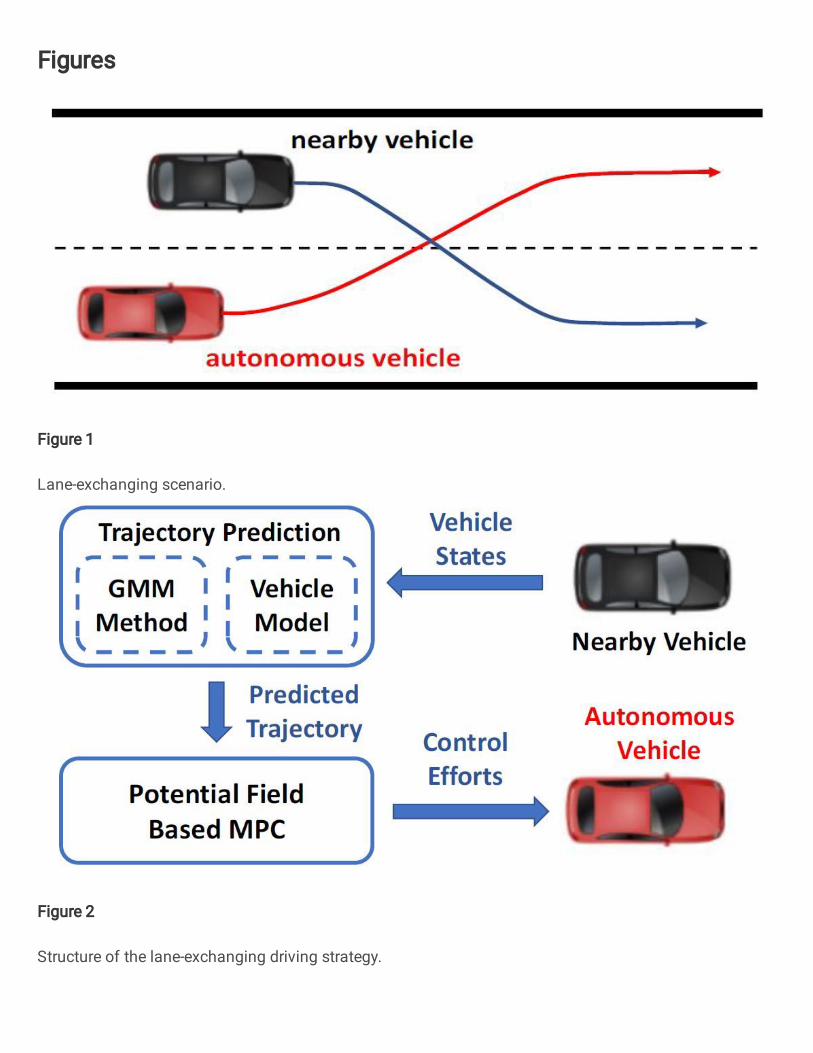
Fig. 1. Lane-exchanging scenario.

autonomous vehicle

nearby vehicle

Lane-Exchanging Driving Strategy for Autonomous Vehicle via Trajectory Prediction and Model Predictive Control

Yimin Chen1,2, Huilong Yu2*, Jinwang Zhang2, Dongpu Cao2 1. The School of Marine Science and Technology Northwestern Polytechnical University, Xi’an, China

2. Department of Mechanical and Mechatronics Engineering University of Waterloo, Ontario N2L3G1, Canada

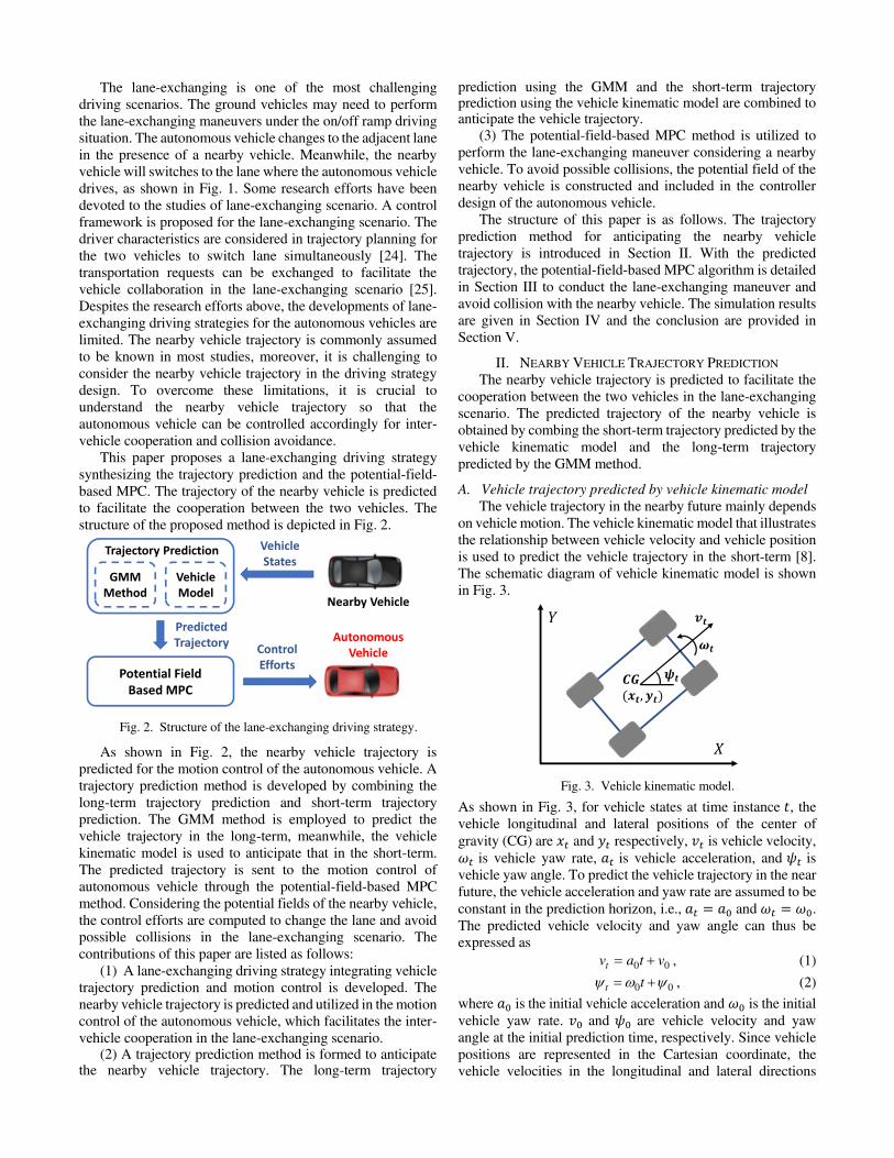
The lane-exchanging is one of the most challenging driving scenarios. The ground vehicles may need to perform the lane-exchanging maneuvers under the on/off ramp driving situation. The autonomous vehicle changes to the adjacent lane in the presence of a nearby vehicle. Meanwhile, the nearby vehicle will switches to the lane where the autonomous vehicle drives, as shown in Fig. 1. Some research efforts have been devoted to the studies of lane-exchanging scenario. A control framework is proposed for the lane-exchanging scenario. The driver characteristics are considered in trajectory planning for the two vehicles to switch lane simultaneously [24]. The transportation requests can be exchanged to facilitate the vehicle collaboration in the lane-exchanging scenario [25]. Despites the research efforts above, the developments of lane- exchanging driving strategies for the autonomous vehicles are limited. The nearby vehicle trajectory is commonly assumed to be known in most studies, moreover, it is challenging to consider the nearby vehicle trajectory in the driving strategy design. To overcome these limitations, it is crucial to understand the nearby vehicle trajectory so that the autonomous vehicle can be controlled accordingly for inter- vehicle cooperation and collision avoidance.

This paper proposes a lane-exchanging driving strategy synthesizing the trajectory prediction and the potential-field-based MPC. The trajectory of the nearby vehicle is predicted to facilitate the cooperation between the two vehicles. The structure of the proposed method is depicted in Fig. 2.

Fig. 2. Structure of the lane-exchanging driving strategy.

As shown in Fig. 2, the nearby vehicle trajectory is predicted for the motion control of the autonomous vehicle. A trajectory prediction method is developed by combining the long-term trajectory prediction and short-term trajectory prediction. The GMM method is employed to predict the vehicle trajectory in the long-term, meanwhile, the vehicle kinematic model is used to anticipate that in the short-term. The predicted trajectory is sent to the motion control of autonomous vehicle through the potential-field-based MPC method. Considering the potential fields of the nearby vehicle, the control efforts are computed to change the lane and avoid possible collisions in the lane-exchanging scenario. The contributions of this paper are listed as follows:

(1) A lane-exchanging driving strategy integrating vehicle trajectory prediction and motion control is developed. The nearby vehicle trajectory is predicted and utilized in the motion control of the autonomous vehicle, which facilitates the inter- vehicle cooperation in the lane-exchanging scenario.

(2) A trajectory prediction method is formed to anticipate the nearby vehicle trajectory. The long-term trajectory

prediction using the GMM and the short-term trajectory prediction using the vehicle kinematic model are combined to anticipate the vehicle trajectory.

(3) The potential-field-based MPC method is utilized to perform the lane-exchanging maneuver considering a nearby vehicle. To avoid possible collisions, the potential field of the nearby vehicle is constructed and included in the controller design of the autonomous vehicle.

The structure of this paper is as follows. The trajectory prediction method for anticipating the nearby vehicle trajectory is introduced in Section II. With the predicted trajectory, the potential-field-based MPC algorithm is detailed in Section III to conduct the lane-exchanging maneuver and avoid collision with the nearby vehicle. The simulation results are given in Section IV and the conclusion are provided in Section V.

II. NEARBY VEHICLE TRAJECTORY PREDICTION The nearby vehicle trajectory is predicted to facilitate the

cooperation between the two vehicles in the lane-exchanging scenario. The predicted trajectory of the nearby vehicle is obtained by combing the short-term trajectory predicted by the vehicle kinematic model and the long-term trajectory predicted by the GMM method.

A. Vehicle trajectory predicted by vehicle kinematic model

The vehicle trajectory in the nearby future mainly depends on vehicle motion. The vehicle kinematic model that illustrates the relationship between vehicle velocity and vehicle position is used to predict the vehicle trajectory in the short-term [8]. The schematic diagram of vehicle kinematic model is shown in Fig. 3.

Fig. 3. Vehicle kinematic model.

As shown in Fig. 3, for vehicle states at time instance 𝑡, the vehicle longitudinal and lateral positions of the center of gravity (CG) are 𝑥𝑡 and 𝑦𝑡 respectively, 𝑣𝑡 is vehicle velocity, 𝜔𝑡 is vehicle yaw rate, 𝑎𝑡 is vehicle acceleration, and 𝜓𝑡 is vehicle yaw angle. To predict the vehicle trajectory in the near future, the vehicle acceleration and yaw rate are assumed to be constant in the prediction horizon, i.e., 𝑎𝑡 = 𝑎0 and 𝜔𝑡 = 𝜔0. The predicted vehicle velocity and yaw angle can thus be expressed as

0 0tv a t v , (1)

0 0t t , (2)

where 𝑎0 is the initial vehicle acceleration and 𝜔0 is the initial vehicle yaw rate. 𝑣0 and 𝜓0 are vehicle velocity and yaw angle at the initial prediction time, respectively. Since vehicle positions are represented in the Cartesian coordinate, the vehicle velocities in the longitudinal and lateral directions

Potential Field

Based MPC

GMM

Method

Trajectory Prediction

Nearby Vehicle

Autonomous

Vehicle

Vehicle

States

Control

Efforts

Vehicle

Model

Predicted

Trajectory

need to be computed. According to the vehicle kinematic model, the vehicle velocity can be computed as

cosxt t tv v , (3)

sinyt t tv v , (4)

where 𝑣𝑥𝑡 and 𝑣𝑦𝑡 are vehicle longitudinal velocity and lateral

velocity at the prediction time 𝑡, respectively. Let the initial vehicle longitudinal and lateral positions be 𝑥0 and 𝑦0.Then, the vehicle trajectory at the future time 𝑡 can be obtained by integrating the velocities 𝑣𝑥𝑡 and 𝑣𝑦𝑡 [9], which are

0 0 00 0 02 2

0 00 0

cos sin cos sintt t t

a v a vx x

, (5)

0 0 00 0 02 2

0 00 0

sin cos sin costt t t

a v a vy y

, (6)

The predicted trajectory consists of vehicle longitudinal position 𝑥𝑡 and lateral position 𝑦𝑡, which can be written as

1( ) ( , )t tTr t x y , (7)

where 𝑇𝑟1 𝑡 is the trajectory predicted by the vehicle kinematic model. The constant yaw rate and acceleration model is employed for the short-term trajectory prediction via equations (5) and (6).

B. Vehicle trajectory predicted by GMM

Vehicle trajectory in the long-term relates to the drivers’ intention and maneuver. In the lane-exchanging scenario, the nearby vehicle will change to the lane where the autonomous vehicle drives. Therefore, the long-term trajectory of the nearby vehicle can be anticipated by learning the historical driving data of the lane-change maneuver when the drivers’ lane-change intention is identified. As this study mainly focuses on the vehicle trajectory prediction, the lane-change intention of the nearby vehicle is assumed to be given or anticipated by other advanced algorithms [26].

For the purpose of predicting vehicle trajectory in the long-term, it is assumed the future vehicle trajectory depends on the historical vehicle trajectory. Therefore, the probability distributions of the historical trajectory is utilized to infer that of the future trajectory. Considering its advantages of approximating various kinds of probability distribution, the GMM method is used to represent the probability distribution of vehicle trajectories. The evolution of vehicle trajectory is thus regarded as a Gaussian process, and the Gaussian regression can be adopted for vehicle trajectory prediction. The procedures of vehicle trajectory prediction consist of two stages: the GMM model is firstly obtained by learning the lane-change driving data; Then the future vehicle trajectory can be anticipated via the conditional Gaussian distribution, given the historical vehicle trajectory.

In order to obtain a uniform representation of the vehicle trajectory and ensure the path smoothness, the vehicle trajectory is represented by Chebyshev polynomial to facilitate the trajectory prediction [7]. The historical vehicle trajectory can be expressed as

1

( ) ( )m

h hi hi

i

Tr t x Ch t

, (8)

where 𝑇𝑟ℎ 𝑡 is the historical vehicle trajectory. 𝐶ℎℎ𝑖 𝑡 is the Chebyshev polynomial of the historical trajectory evaluated at

time step t. The subscript 𝑖 indicates the order of the Chebyshev polynomial and 𝑖 = 1 2 … 𝑚. 𝑥ℎ𝑖 is the Chebyshev polynomial coefficient and the coefficient vector of the historical trajectory is xℎ = [𝑥ℎ1 𝑥ℎ2 … 𝑥ℎ𝑚]𝑇 . Based on equation (8), the historical vehicle trajectory is decomposed as the Chebyshev polynomials and their coefficients. The polynomial coefficients are used to represent the historical vehicle trajectory. Similarly, the future vehicle trajectory can be expressed in the same way. The coefficient vector of the

future vehicle trajectory is x𝑓 = [𝑥𝑓1 𝑥𝑓2 … 𝑥𝑓𝑚]𝑇. Since the

vehicle trajectory is represented by polynomial coefficients, the vehicle trajectory prediction can be converted into the prediction of the polynomial coefficients.

Owing to the relationship between the historical and future vehicle trajectories, together with the Chebyshev polynomials representation, the future vehicle trajectory can be predicted by computing the future polynomial coefficients using the historical polynomial coefficient. The coefficient vector xℎ of the historical trajectory is used as the input feature, and the prediction output is the coefficient vector x𝑓 of the future

vehicle trajectory. In order to describe the relationship between the history and the future coefficients, a state vector is defined as

x

xh

f

GS

, (9)

The distribution of the state vector 𝐺𝑆 is assumed as a Gaussian mixture distribution, which is written as

1

( , )n

k k k

k

GS

, (10)

where 𝑢𝑘 and Σ𝑘 are the mean and the covariance of the Gaussian component 𝑘. 𝜔𝑘 is the weight of the corresponding Gaussian component. 𝑛 is the number of the Gaussian components and a single Gaussian component 𝑘 can be written as

,

,

k h

kk f

, (11)

, ,

, ,

k h k hf

kk fh k f

. (12)

where the subscript ℎ denotes the history information and the subscript 𝑓 represents the future information. The mean 𝑢𝑘 and covariance Σ𝑘 of the component 𝑘 of the GMM can be obtained by learning the driving dataset. The GMM is utilized to approximate the distribution of the historical and future trajectories.

After inferring the GMM, the state vector 𝐺𝑆 can be approximated. The relationship between the historical trajectory coefficient and the future trajectory coefficient are described by the Gaussian process. Then, the mixture distribution 𝑝 x𝑓|xℎ is used to predict the future trajectory

coefficient x𝑓, given the history trajectory coefficient xℎ. As

the distribution of the polynomial coefficients consists of 𝑛 Gaussian components, the covariance of the Gaussian component 𝑘 of the conditional mixture distribution is written as

1

, | , , , ,k f h k f k fh k h k hf , (13)

The mean of the Gaussian component 𝑘 of the conditional mixture distribution can be calculated as

1

, | , , , ,(x )k f h k f k fh k h h k h , (14)

For the Gaussian components 𝑘, the weight the conditional mixture distribution can be computed as

,x ,x

|

,x ,x1

(x | , )

(x | , )

h h

h h

k h k k

k h n

k h k kk

p

p

. (15)

The equations (13) ~ (15) define a full conditional probability density function of the polynomial coefficient of the future trajectory. The conditional mixture distribution 𝑝 x𝑓|xℎ of

the future trajectory coefficients can be given as

| , | , |

1

( | ) ( , )n

f h k h k f h k f h

k

p x x

. (16)

From equation (16), the conditional mixture distribution of the polynomial coefficients of the future trajectory can be obtained. The mean and covariance of the conditional probability distribution are the combination of the n Gaussian components, which can be written as

, | | , |

1

n

f h k h k f h

k

, (17)

, | | , | , | , | , |

1

( ( )( ) )K

Tf h k h k k f h f h k f h f h

k

.

(18) The future vehicle trajectory is predicted by computing the

distribution of the polynomial coefficients of the future trajectory, which is approximated by the conditional mixture distribution. Since the vehicle trajectory is represented by the Chebyshev polynomial, the future vehicle trajectory can be given as

2( ) ( ) x fTr t Ch t (19)

where 𝑇𝑟2 𝑡 is the predicted vehicle trajectory. x𝑓 is the

predicted coefficient vector of the Chebyshev polynomial. 𝐶ℎ 𝑡 is the Chebyshev polynomial evaluated at time 𝑡. The future vehicle trajectory can be predicted through above procedures.

C. Trajectory prediction integration The short-term trajectory prediction and the long-term

trajectory prediction are integrated to obtain the final predicted vehicle trajectory. The vehicle kinematic model is accurate in the short-term prediction, meanwhile, the GMM method emphases on the long-term prediction. To obtain the final trajectory prediction, a weighting function is utilized to combine the predicted trajectories in both the short-term and long-term.

Considering the smoothness of vehicle trajectory, the cubic spline function 𝑓 𝑡 is used to construct the weighing function that integrates the two predicted trajectories. The weighing function is defined as a cubic spline within the prediction horizon [0 𝑇] and 0 ≤ 𝑓 𝑡 ≤ 1 . Then, the prediction trajectory can be written as

1 2( ) ( ) ( ) (1 ( )) ( )Tr t f t Tr t f t Tr t . (20)

The final predicted trajectory is represented by 𝑇𝑟 𝑡 . With the prediction time 𝑡 increases from 0 to 𝑇 , the weighting function 𝑓 𝑡 is decreasing from 1 to 0. At the beginning of the trajectory prediction, the short-term predicted trajectory 𝑇𝑟1 𝑡 dominates the trajectory prediction and the weighting function 𝑓 𝑡 is close to 1. As the prediction time increase, the predicted trajectory is close to the long-term predicted trajectory 𝑇𝑟2 𝑡 which means the weighting function 𝑓 𝑡 approaches to 0.

III. POTENTIAL FIELD BASED MODEL PREDICTIVE CONTROL With the predicted nearby vehicle trajectory, the potential-

field-based MPC algorithm is used to perform the lane-exchanging maneuver and cooperate simultaneously with the nearby vehicle.

A. Vehicle system model

A control-oriented vehicle model is formed for the controller design. The bicycle vehicle model that simplifies the model complexity while preserving accuracy is utilized to describe vehicle motion on the ground. The bicycle vehicle model is illustrated in Fig. 4.

Fig. 4. Vehicle dynamic model.

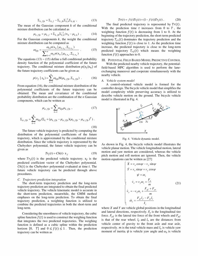
As shown in Fig. 4, the bicycle vehicle model illustrates the vehicle planar motion. The vehicle longitudinal motion, lateral motion and yaw motion are considered, whereas the vehicle pitch motion and roll motion are ignored. Then, the vehicle motion equations can be written as [27]

cos sin

sin cos

x y

x y

z

xx y z

yf yr

y x z

yf f yr r

z

z

X v v

Y v v

Fv v

m

F Fv v

m

F l F l

I

(21)

where and are vehicle global positions in the longitudinal and lateral directions, respectively. 𝐹𝑥 is the longitudinal tire force. 𝐹𝑦𝑓 is the lateral tire force of the front wheels and 𝐹𝑦𝑓

is that of the rear wheel. 𝑙𝑓 and 𝑙𝑟 are the distances from

vehicle center of gravity to the front axle and rear axle, respectively. 𝑚 is the total vehicle mass and 𝐼𝑧 is vehicle yaw moment of inertia. 𝜓 is vehicle yaw angle and 𝜔𝑧 is vehicle

yaw rate. 𝑣𝑥 and 𝑣𝑦 are vehicle longitudinal and lateral

velocity, respectively. In the lane-exchanging scenario, the vehicle yaw angle is

assumed small [24]. Therefore, we can have the conditions cos𝜓 ≈ 1 and sin𝜓 ≈ 𝜓. The vehicle global position can then be simplified as

x yX v v , (22)

x yY v v , (23)

Considering the normal driving conditions studied in this paper, the linear tire model is used to compute the lateral tire forces, which are

( )y f z

yf f

x

v lF C

v

, (24)

y r z

yf r

x

v lF C

v

, (25)

where 𝛿 is the steering angle of the front wheel. 𝐶𝑓 and 𝐶𝑟 are

the cornering stiffness of the front axle and the rear axle, respectively.

By substituting equations (23) ~ (25) into equation (21), the vehicle system model in equation (21) can be rewritten into the state space representation, which is

A Bu

C

, (26)

where the state vector is 𝜉 and 𝜉 = [ 𝑣𝑥 𝑣𝑦 𝜓 𝜔𝑧]𝑇. The

system output would be 𝜂 = [ 𝜓 𝑣𝑥]𝑇. The control inputs are the steering angle and the longitudinal tire force, i.e., 𝑢 =[𝛿 𝐹𝑥]𝑇. A is the system matrix, B is the control matrix, and C

is the output matrix. The above matrices can be expressed as

2 2

0 1 0 0 0

0 0 0 0 0

0 0 0 1 0

0 0 0 0

0 0 0 0 0 1

0 0 0 0

y

y

x

f r r r f f

x

x x

r r f f r r f f

z x z x

v

v

v

C C C l C lA v

mv mv

l C l C l C l C

I v I v

,

10 0 0 0 0

0 0 0 0

T

f f f

mB

C l C

m m

,

0 0 1 0 0 0

0 0 0 0 1 0

0 1 0 0 0 0

C

. (27)

The vehicle model in equation (26) is utilized as the predictive model of the MPC algorithm. Under the MPC scheme, the vehicle system is discretized as

( 1) ( ) ( )

( ) ( )k k

k

k A k B u k

k C k

. (28)

where 𝐴𝑘 is the discretized system matrix and 𝐴𝑘 = 𝐼 + 𝑇𝑠𝐴. 𝐵𝑘 is the discretized control matrix and 𝐵𝑘 = 𝑇𝑠𝐵. 𝑇𝑠 is the sampling time. The discretized output matrix is 𝐶𝑘 . The incremental of the control efforts is written as ∆𝑢 𝑘 that satisfies the condition ∆𝑢 𝑘 = 𝑢 𝑘 − 𝑢 𝑘 − 1 . B. Potential fields

The autonomous vehicle has to cooperate with the nearby vehicle for collision avoidance in the lane-exchanging scenario. The nearby vehicle is thus regarded as a moving obstacle that needs to be avoided when the autonomous vehicle changes to the other lane. By predicting the nearby vehicle trajectory, the potential field of the nearby vehicle is constructed and considered in the controller design, in order to avoid possible collisions between the two vehicles. The potential field of the nearby vehicle can be written as [28]

( , )

( , )o

b

s s

aU X Y

X YSD

X Y

, (29)

where 𝑎 is the intensity parameter and 𝑏 is the shape parameter of the potential field of the nearby vehicle. ∆ and ∆ are the relative distances between two vehicles in the longitudinal and the lateral directions, respectively. The term 𝑆𝐷 ∙ represents the signed distance that represents the relative position between the two vehicles and is detailed in [29]. 𝑠 is the safe distance in the longitudinal direction and 𝑠 is that in the lateral direction, which are defined as

2

0 02

xs x

n

vX X v T

a

， (30)

2

0 0( sin sin )2

y

s x nx

n

vY Y v v T

a

， (31)

where 𝑣𝑥𝑛 is the velocity of the nearby vehicle. Δ𝑣𝑥 and Δ𝑣𝑦

are the longitudinal and lateral approaching velocity, respectively. 0 is the minimum allowed longitudinal distance and 0 is the minimum allowed lateral distance. 𝑎𝑛 represents the vehicle acceleration. 𝑇0 is the safe time gap and 𝜃 is the heading angle between the two vehicles. The potential field increases as the autonomous approaches to the nearby vehicle. The autonomous vehicle is preferred to drive along the low potential area and avoid the high potential area, so that the autonomous vehicle can avoid the nearby vehicle in the lane-exchanging scenarios.

Besides the potential field of the nearby vehicle, the potential field of the road boundary is defined to prevent the vehicle from leaving the lane. The potential field of the road boundary is written as

2 ( , )( ( , ) )( , )

( , )0

R aR R aR

R a

SD X Y Da SD X Y DU X Y

SD X Y D

,

(32) where 𝑆𝐷𝑅 ∙ is the singed distance between the autonomous vehicle and the road boundary. 𝐷𝑎 is the safety distance from the lane boundary. 𝑎𝑅 is the intensity parameter. With the potential field defined for the lane boundary, the autonomous vehicle are prevented from leaving the lane.

The functions of the potential fields are nonlinear and nonconvex, so as the problem of controller design. Its solution

is thus time consuming and computational expensive. In order to reduce the computational cost, the potential fields are approximated by convex functions via coordinate transformation. The controller design problem can thus be converted into a convex quadratic optimization problem. The convex processes are detailed in [30] and thus omitted here.

C. Cost function and constraints

The control objective is to avoid the nearby vehicle while performing the lane-change maneuver at the same time. The lateral motion and longitudinal motion of the autonomous vehicle have to be manipulated simultaneously. As the autonomous will change to the adjacent lane where the nearby vehicle drives, the desired trajectory is the centerline of the adjacent lane. Therefore, the cost function considering the nearby vehicle, the road boundaries, and the trajectory tracking errors is written as

1

1 0

1

( ( | ) ( | )) ( | )

( | ) ( | )

N N

o R c Rk k

N

des Qk

J U t k t U t k t u t k t

t k t t k t

, (33)

where 𝑈0 𝑡 + 𝑘|𝑡 is the potential fields of the nearby vehicle of time step 𝑡 + 𝑘 which is computed at time step 𝑡, similar to the potential filed of the road boundary 𝑈𝑅 𝑡 + 𝑘|𝑡 . The control effort is 𝑢𝑐 𝑡 + 𝑘|𝑡 and its corresponding weighting matrix is 𝑅. 𝜂𝑑𝑒𝑠 𝑡 + 𝑘|𝑡 is the desired system outputs that contains the lateral position and the yaw angle of the centerline of the target lane, as well as the desired velocity. 𝑄 is the weighting matrix of the trajectory tracking error.

After defining the cost function, the control efforts can be computed by solving the receding horizon optimization problem. The vehicle system model and the control saturation are considered as the constraints of the optimization problem. Meanwhile, the vehicle states needs to be confined in the reasonable ranges to ensure the driving safety and ride comfort. Then, the optimization problem can be expressed as

( | ),..., ( 1| )

min ( ( | ), ( | ))u t k t u t k N t

J t k t u t k t

s.t. ( 1| ) ( | ) ( | )k k ct k t A t k t B u t k t

( | ) ( | )kt k t C t k t

min max( | )c c cu u t k t u

min max( | )c cu u t k t u

( 1| ) ( | ) ( | )u t k t u t k t u t k t

for k = 0, 2, 3, …, N-1. (34) where 𝑢 𝑡 + 𝑘|𝑡 represents the control effort of the time step 𝑡 + 𝑘 computed at time step 𝑡. The 𝑢𝑐min and 𝑢𝑐max are the lower bound and the upper bound of the control effort. Considering the actuator saturation, the minimum and maximum steering angle are 𝛿min and 𝛿max , the minimum and maximum driving torque are 𝑇min and 𝑇max . Then the constraints of the control efforts are

min min minT

cu T , max max maxT

cu T , (35)

Similarly, the constraints of the incremental of the control efforts are considered. The ∆𝑢 𝑡 + 𝑘|𝑡 is confined by its lower bound ∆𝑢𝑐min and its upper bound ∆𝑢𝑐max. Define the minimum and maximum steering angle between two steps as

∆𝛿min and ∆𝛿max, and the minimum and maximum driving torque between two steps as ∆𝑇min and ∆𝑇max . Then the constraints of ∆𝑢 𝑡 + 𝑘|𝑡 are bounded as

min min minT

cu T , max max maxT

cu T ,(36)

Under the MPC scheme, a sequence of control efforts are computed, whereas only the first one is sent to drive the autonomous vehicle. More details about the MPC algorithm can be found in [31].

IV. DRIVING DATA AND SIMULATION VALIDATION

The on-road driving data from the Highway Drone Dataset is used to verify the trajectory prediction method. The proposed method is used to anticipate the trajectory of the nearby vehicle. Based on the predicted trajectory, the potential-field-based MPC approach is then utilized to conduct the lane-exchanging maneuver and avoid possible collisions. The designed control method is validated through simulation studies.

A. Trajectory prediction results

The developed vehicle trajectory prediction method is verified through the Highway Drone Dataset that contains naturalistic vehicle trajectories recorded on German Highway [32]. The vehicle trajectory, including vehicle type, size and maneuver, is collected using a drone from the aerial perspective. The vehicle positions are extracted via the state-of-the-art computer vision algorithms. By learning the on-road driving data, the vehicle trajectory can be anticipated by the proposed method.

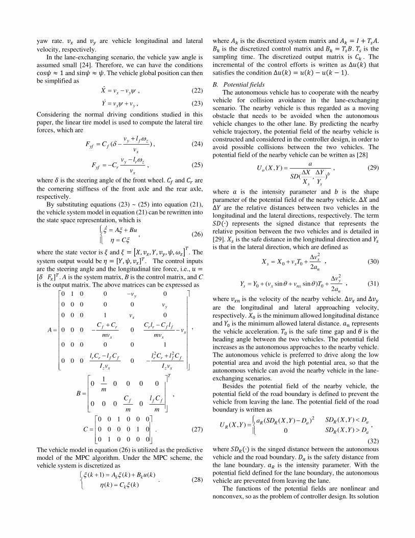
The vehicle trajectory is predicted at different time instance after the start of lane change. Since the nearby vehicle changes to the adjacent lane in the lane-exchanging scenario, the start of lane-change is defined as the instance when the vehicle position is around the centerline of its original lane. The historical trajectory is used to predict the future trajectory for 4 s ahead. The trajectory prediction results at the time instance 0.4 s, 1.4 s, and 2.4 s after the start of lane-change are shown in the following figures.

Fig. 5 shows the vehicle trajectory that is predicted at 0.4 s after the start of lane-change. The trajectory prediction is accurate at the beginning of the prediction. The prediction error increases with the prediction time and reaches to 0.2 at the longitudinal position 150 m. The final trajectory has smaller errors than the trajectories predicted either by the GMM method or the vehicle mode.

Fig. 5. Trajectory Prediction at 0.4 s after the start of lane

change.

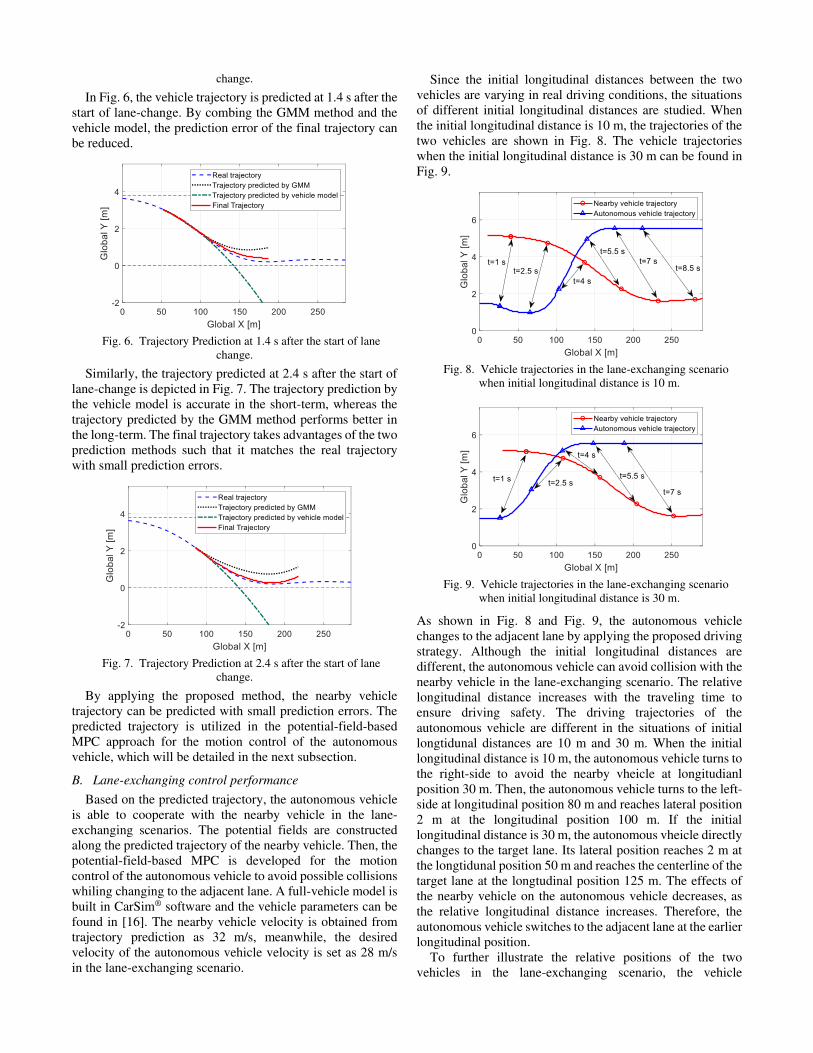
In Fig. 6, the vehicle trajectory is predicted at 1.4 s after the start of lane-change. By combing the GMM method and the vehicle model, the prediction error of the final trajectory can be reduced.

Fig. 6. Trajectory Prediction at 1.4 s after the start of lane

change.

Similarly, the trajectory predicted at 2.4 s after the start of lane-change is depicted in Fig. 7. The trajectory prediction by the vehicle model is accurate in the short-term, whereas the trajectory predicted by the GMM method performs better in the long-term. The final trajectory takes advantages of the two prediction methods such that it matches the real trajectory with small prediction errors.

Fig. 7. Trajectory Prediction at 2.4 s after the start of lane

change.

By applying the proposed method, the nearby vehicle trajectory can be predicted with small prediction errors. The predicted trajectory is utilized in the potential-field-based MPC approach for the motion control of the autonomous vehicle, which will be detailed in the next subsection.

B. Lane-exchanging control performance

Based on the predicted trajectory, the autonomous vehicle is able to cooperate with the nearby vehicle in the lane-exchanging scenarios. The potential fields are constructed along the predicted trajectory of the nearby vehicle. Then, the potential-field-based MPC is developed for the motion control of the autonomous vehicle to avoid possible collisions whiling changing to the adjacent lane. A full-vehicle model is built in CarSim® software and the vehicle parameters can be found in [16]. The nearby vehicle velocity is obtained from trajectory prediction as 32 m/s, meanwhile, the desired velocity of the autonomous vehicle velocity is set as 28 m/s in the lane-exchanging scenario.

Since the initial longitudinal distances between the two vehicles are varying in real driving conditions, the situations of different initial longitudinal distances are studied. When the initial longitudinal distance is 10 m, the trajectories of the two vehicles are shown in Fig. 8. The vehicle trajectories when the initial longitudinal distance is 30 m can be found in Fig. 9.

Fig. 8. Vehicle trajectories in the lane-exchanging scenario

when initial longitudinal distance is 10 m.

Fig. 9. Vehicle trajectories in the lane-exchanging scenario

when initial longitudinal distance is 30 m.

As shown in Fig. 8 and Fig. 9, the autonomous vehicle changes to the adjacent lane by applying the proposed driving strategy. Although the initial longitudinal distances are different, the autonomous vehicle can avoid collision with the nearby vehicle in the lane-exchanging scenario. The relative longitudinal distance increases with the traveling time to ensure driving safety. The driving trajectories of the autonomous vehicle are different in the situations of initial longtidunal distances are 10 m and 30 m. When the initial longitudinal distance is 10 m, the autonomous vehicle turns to the right-side to avoid the nearby vheicle at longitudianl position 30 m. Then, the autonomous vehicle turns to the left-side at longitudinal position 80 m and reaches lateral position 2 m at the longitudinal position 100 m. If the initial longitudinal distance is 30 m, the autonomous vheicle directly changes to the target lane. Its lateral position reaches 2 m at the longtidunal position 50 m and reaches the centerline of the target lane at the longtudinal position 125 m. The effects of the nearby vehicle on the autonomous vehicle decreases, as the relative longitudinal distance increases. Therefore, the autonomous vehicle switches to the adjacent lane at the earlier longitudinal position.

To further illustrate the relative positions of the two vehicles in the lane-exchanging scenario, the vehicle

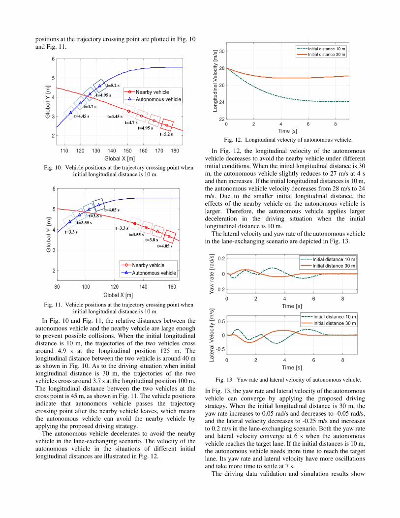
positions at the trajectory crossing point are plotted in Fig. 10 and Fig. 11.

Fig. 10. Vehicle positions at the trajectory crossing point when

initial longitudinal distance is 10 m.

Fig. 11. Vehicle positions at the trajectory crossing point when

initial longitudinal distance is 10 m.

In Fig. 10 and Fig. 11, the relative distances between the autonomous vehicle and the nearby vehicle are large enough to prevent possible collisions. When the initial longitudinal distance is 10 m, the trajectories of the two vehicles cross around 4.9 s at the longitudinal position 125 m. The longitudinal distance between the two vehicle is around 40 m as shown in Fig. 10. As to the driving situation when initial longitudinal distance is 30 m, the trajectories of the two vehicles cross around 3.7 s at the longitudinal position 100 m. The longitudinal distance between the two vehicles at the cross point is 45 m, as shown in Fig. 11. The vehicle positions indicate that autonomous vehicle passes the trajectory crossing point after the nearby vehicle leaves, which means the autonomous vehicle can avoid the nearby vehicle by applying the proposed driving strategy.

The autonomous vehicle decelerates to avoid the nearby vehicle in the lane-exchanging scenario. The velocity of the autonomous vehicle in the situations of different initial longitudinal distances are illustrated in Fig. 12.

Fig. 12. Longitudinal velocity of autonomous vehicle.

In Fig. 12, the longitudinal velocity of the autonomous vehicle decreases to avoid the nearby vehicle under different initial conditions. When the initial longitudinal distance is 30 m, the autonomous vehicle slightly reduces to 27 m/s at 4 s and then increases. If the initial longitudinal distances is 10 m, the autonomous vehicle velocity decreases from 28 m/s to 24 m/s. Due to the smaller initial longitudinal distance, the effects of the nearby vehicle on the autonomous vehicle is larger. Therefore, the autonomous vehicle applies larger deceleration in the driving situation when the initial longitudinal distance is 10 m.

The lateral velocity and yaw rate of the autonomous vehicle in the lane-exchanging scenario are depicted in Fig. 13.

Fig. 13. Yaw rate and lateral velocity of autonomous vehicle.

In Fig. 13, the yaw rate and lateral velocity of the autonomous vehicle can converge by applying the proposed driving strategy. When the initial longitudinal distance is 30 m, the yaw rate increases to 0.05 rad/s and decreases to -0.05 rad/s, and the lateral velocity decreases to -0.25 m/s and increases to 0.2 m/s in the lane-exchanging scenario. Both the yaw rate and lateral velocity converge at 6 s when the autonomous vehicle reaches the target lane. If the initial distances is 10 m, the autonomous vehicle needs more time to reach the target lane. Its yaw rate and lateral velocity have more oscillations and take more time to settle at 7 s.

The driving data validation and simulation results show

t=4.45 s

t=4.7 s

t=4.95 s

t=5.2 s

t=4.45 s

t=4.7 s

t=4.95 s

t=5.2 s

t=3.55 s

t=4.05 s

t=3.8 s

t=3.3 s t=3.3 s

t=3.55 s t=3.8 s

t=4.05 s

that the autonomous vehicle can avoid the nearby vehicle in the lane-exchanging scenario by applying the proposed driving strategy.

V. CONCLUSIONS This paper proposes a lane-exchanging driving strategy by

combining the trajectory prediction of the nearby vehicle and the motion control of the autonomous vehicle. The GMM method and the vehicle kinematic mode is utilized to predict the trajectory of the nearby vehicle. Based on the predicted trajectory, the potential-field-based MPC approach is designed for the autonomous vehicle to perform the lane-exchanging maneuver and cooperate with the nearby vehicle. The potential field of the nearby vehicle is considered in the controller design to avoid possible collisions. The proposed driving strategy is validated through the on-road driving data and the simulations. The results shows the autonomous vehicle can avoid the nearby vehicle in the lane-exchanging scenarios. Only one nearby vehicle is considered in this study for simplicity. In the following works, the complex driving situations involving multiple nearby vehicles will be investigated.

Acknowledgements

Not applicable. Authors’ Contributions

YMC and HLY conceived and proposed the idea of the lane-exchanging driving problem; YMC developed the vehicle model and devised the MPC based controller; HLY and JWZ devised the algorithms of the trajectory prediction; YMC prepared the manuscript, HLY and DPC assisted with the manuscript revision. All authors read and approved the final manuscript.

Funding This work is partly supported by the State Key Laboratory of Automotive Safety and Energy under Project No. KF2014. Competing Interests The authors declare no competing financial interests.

REFERENCES [1] D. González, J. Pérez, V. Milanés, and F. Nashashibi, "A Review of

Motion Planning Techniques for Automated Vehicles." IEEE Trans.

Intelligent Transportation Systems, vol. 17, (4), pp. 1135-1145, 2016. [2] P. Koopman, and M. Wagner, Autonomous vehicle safety: An

interdisciplinary challenge. IEEE Intelligent Transportation Systems

Magazine, vol. 9, no. 1, pp: 90-96, 2017. [3] D. J. Fagnant, K. M. Kockelman, and P. Bansal, Operations of shared

autonomous vehicle fleet for Austin, Texas, market. Transportation Research Record, vol. 2563, no. 1, pp. 98-106, 2015.

[4] N. Li, D. W. Oyler, M. Zhang, Y. Yildiz, I. Kolmanovsky, and A. R. Girard, Game theoretic modeling of driver and vehicle interactions for verification and validation of autonomous vehicle control systems. IEEE Transactions on control systems technology, vol. 26, no. 5, pp: 1782-1797, 2017.

[5] Y. Chen and J. Wang, “Trajectory tracking control for autonomous vehicles in different cut-in scenarios,” Proceedings of the 2019 American Control Conference, pp. 4878-4883, 2019.

[6] N. Deo, A. Rangesh, M. M. Trivedi. "How would surround vehicles move? a unified framework for maneuver classification and motion prediction." IEEE Transactions on Intelligent Vehicles, vol. 3, no. 2, pp: 129-140, 2018.

[7] J. Wiest, M. Hoffken, U. Krebel, and K. Dietmayer, "Probabilistic Trajectory Prediction with Gaussian Mixture Models," IEEE Intelligent

Vehicles Symposium, pp: 141-146, 2012. [8] A. Houenou, P. Bonnifait, V. Cherfaoui, and W. Yao. "Vehicle

trajectory prediction based on motion model and maneuver recognition." IEEE/RSJ international conference on intelligent robots

and systems, pp. 4363-4369, 2013. [9] G. Xie, H. Gao, L. Qian, B. Huang, K. Li, and J. Wang. "Vehicle

trajectory prediction by integrating physics-and maneuver-based approaches using interactive multiple models." IEEE Transactions on

Industrial Electronics, vol. 65, no. 7, pp: 5999-6008, 2017. [10] A. Khosroshahi, E. Ohn-Bar, and M. M. Trivedi. Surround vehicles

trajectory analysis with recurrent neural networks. In 2016 IEEE 19th

International Conference on Intelligent Transportation Systems, pp. 2267-2272, 2016.

[11] Y. Chen, C. Hu and J. Wang, “Motion planning with velocity prediction and composite nonlinear feedback tracking control for lane-change strategy of autonomous vehicles,” IEEE Trans. on Intelligent Vehicles. 2019. DOI: 10.1109/TIV.2019.2955366

[12] Xing, Yang, and Chen Lv. "Dynamic State Estimation for the Advanced Brake System of Electric Vehicles by using Deep Recurrent Neural Networks." IEEE Transactions on Industrial Electronics, 2019. DOI:10.1109/TIE.2019.2952807

[13] Deng, Zejian, Duanfeng Chu*, Chaozhong Wu, Yi He, Jian Cui. Curve Safe Speed Model Considering Driving Style Based on Driver Behaviour Questionnaire. Transportation Research Part F: Psychology and Behaviour, vol.65, pp.536-547, 2019.

[14] Li, Mingjun, Haotian Cao, Xiaolin Song, Yanjun Huang, Jianqiang Wang, and Zhi Huang. "Shared control driver assistance system based on driving intention and situation assessment." IEEE Transactions on Industrial Informatics, vol. 14, no. 11 pp: 4982-4994, 2018.

[15] G. Li, Y. Wang, F. Zhu, X. Sui, N. Wang, X. Qu*, P. Green, “Drivers’ Visual Scanning Behavior at Signalized and Unsignalized Intersections: A Naturalistic Driving Study in China”, Journal of Safety Research, DOI:10.1016/j.jsr.2019.09.012, 2019

[16] Y. Chen, X. Zhang and J. Wang, “Robust vehicle driver assistance control for handover scenarios considering driving performances,” IEEE Trans. on Systems, Man and Cybernetics: Systems (DOI: 10.1109/TSMC.2019.2931484)

[17] Y. Chen, C. Stout, A. Joshi, M. Kuang, and J. Wang, “Driver assistance lateral motion control for in-wheel-motor-driven electric ground vehicles subject to small torque variation,” IEEE Trans. on Veh.

Technol., vol. 67, no. 8, pp. 6838-6850, 2018. [18] Y. Chen, J. Zha and J. Wang, “An autonomous T-intersection driving

strategy considering oncoming vehicles based on connected vehicle technology,” IEEE/ASME Trans. on Mechatronics. (DOI: 10.1109/TMECH.2019.2942769)

[19] Y. Chen, C. Hu and J. Wang, “Human-centered tracking control for autonomous vehicle with driver cut-in behavior prediction,” IEEE

Trans. on Veh. Technol., vol. 68, no.9, pp.8461-8471, 2019. [20] C. Hu, Z. Wang, H. Taghavifar, J. Na, Y. Qin, J. Guo, and C. Wei,

"MME-EKF-Based Path-Tracking Control of Autonomous Vehicles Considering Input Saturation," IEEE Transactions on Vehicular

Technology, 2019. DOI: 10.1109/TVT.2019.2907696. [21] Huilong Yu, Francesco Castelli-Dezza and Federico Cheli, Optimal

Design and Control of 4-IWD Electric Vehicles based on a 14-DOF Vehicle Model, IEEE Transactions on Vehicular Technology, vol. 67, no. 11, pp. 10457-10469. 2018.

[22] H Zhang, W Zhao. Decoupling control of steering and driving system for in-wheel-motor-drive electric vehicle. Mechanical Systems &

Signal Processing, vol. 101, pp:389-404, 2018. [23] H Zhang, W Zhao and J Wang. Fault-tolerant control for electric

vehicles with independently driven in-wheel-motors considering individual driver steering characteristics[J]. IEEE Transactions on Vehicular Technology, vol. 68, no. 5, pp:4527-4536, 2019.

[24] J. Wang, J. Wang, A Framework of Vehicle Trajectory Replanning in Lane Exchanging With Considerations of Driver Characteristics

[25] M. Gansterera, Richard F. Hartl Collaborative vehicle routing: a survey, European Journal of Operational Research, vol.268, no.1, 1-12, 2018.

[26] A. Doshi, and M. M. Trivedi, Tactical driver behavior prediction and intent inference: A review. In 2011 14th International IEEE Conference on Intelligent Transportation Systems, pp. 1892-1897, 2011.

[27] Y. Chen, Y, C. Lu, and W. Chu, "A Cooperative Driving Strategy Based on Velocity Prediction for Connected Vehicles With Robust Path- Following Control." IEEE Internet of Things Journal, vol. no.5, pp 3822-3832. 2020.

[28] H. Wang, Y. Huang, A. Khajepour, Y. Zhang, Y. Rasekhipour, and D. Cao, "Crash mitigation in motion planning for autonomous vehicles." IEEE Transactions on Intelligent Transportation Systems, vol. 20, no. 9, 3313-3323, 2019.

[29] Schulman, J., Ho, J., Lee, A. X., 2013, "Finding Locally Optimal, Collision-Free Trajectories with Sequential Convex Optimization." Robotics: science and systems, Anonymous Citeseer, vol. 9, pp. 1-10. 2013.

[30] Y. Rasekhipour, A. Khajepour, S. K. Chen, and B. Litkouhi, A potential field-based model predictive path-planning controller for autonomous road vehicles. IEEE Transactions on Intelligent Transportation

Systems, vol. 18, no. 5, 1255-1267, 2016. [31] Y. Chen and J. Wang, “In-wheel-motor-driven electric vehicles motion

control methods considering motor thermal protection,” ASME Trans. J. Dyn. Syst. Meas. Control, vol.141, no.1, 2019:011015.

[32] R. Krajewski, J. Bock, L. Kloeker, and L. Eckstein, The highd dataset: A drone dataset of naturalistic vehicle trajectories on german highways for validation of highly automated driving systems. In 2018 21st

International Conference on Intelligent Transportation Systems, pp. 2118-2125, 2018.

Yimin Chen is currently a Postdoctoral Fellow at the Department of Mechanical and Mechatronics Engineering, University of Waterloo, Waterloo, Canada. He received his B.S. degrees in Mechanical Design from Central South University, Hunan, China, in 2012, and his M.S. degrees in Mechanical Engineering from Xi’an Jiaotong University, Xi’an, China in 2015. He obtained his Ph.D. degrees in the Walker Department of Mechanical Engineering at

the University of Texas at Austin, Austin, TX, USA, in 2019. His research interests include automated vehicles, vehicle dynamics and control, and personalized vehicle control systems.

Huilong Yu received the M.Sc. degree in mechanical engineering from the Beijing Institute of Technology, Beijing, China, and the Ph.D. degree in mechanical engineering from Politecnico di Milano, Milano, Italy, in 2013 and 2017, respectively. He is currently a Research Fellow of advanced vehicle engineering with the University of Waterloo, Waterloo, ON, Canada. His research interests include vehicle dynamics, optimal control, decision-making and motion

planning of autonomous vehicles.

Jinwei Zhang received the B.S degree in Worcester Polytechnic Institute, US, double major in Robotics Engineering and Electrical & Computer Engineering. He is currently pursuing M.S. degree in University of Waterloo, major in Mechanical and Mechatronics Engineering, under the supervision of Prof. Dongpu Cao. His current research focuses on the behavior analysis of lane-changing scenario, and the motion prediction of surrounding scenes applied on

Autonomous driving.

Dongpu Cao received the Ph.D. degree from Concordia University, Canada, in 2008. He is currently an Associate Professor and Director of Driver Cognition and Automated Driving (DC-Auto) Lab at University of Waterloo, Canada. His research focuses on vehicle dynamics and control, driver cognition, automated driving and parallel driving, where he has contributed more than 150 publications and 1 US patent. He received the ASME AVTT’2010 Best Paper Award and 2012 SAE Arch T. Colwell Merit Award. Dr. Cao serves as an Associate Editor

for IEEE Transactions on Vehicular Technology, IEEE Transactions on intelligent transportation systems, IEEE/ASME Transactions on

Mechatronics, IEEE Transactions on Industrial Electronics and ASME Journal of Dynamic Systems, Measurement and Control. He has been a Guest Editor for Vehicle System Dynamics, and IEEE TRANSACTIONS ON SMC: SYSTEMS. He has been serving on the SAE International Vehicle Dynamics Standards Committee and a few ASME, SAE, IEEE technical committees, and serves as Co-Chair of IEEE ITSS Technical Committee on Cooperative Driving.

Figures

Figure 1

Lane-exchanging scenario.

Figure 2

Structure of the lane-exchanging driving strategy.

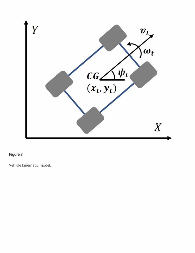
Figure 3

Vehicle kinematic model.

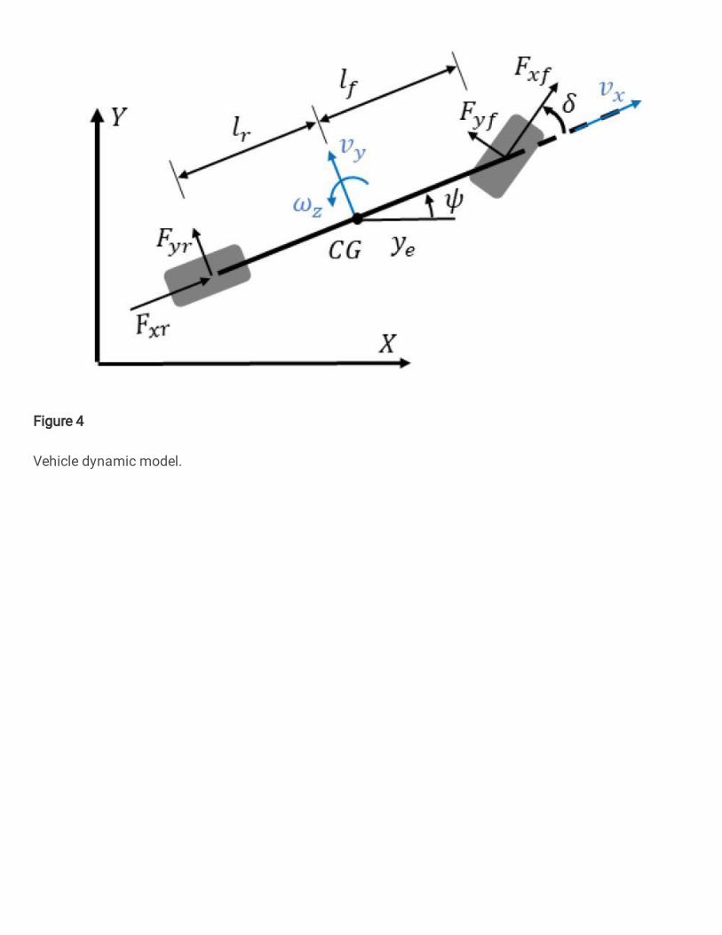
Figure 4

Vehicle dynamic model.

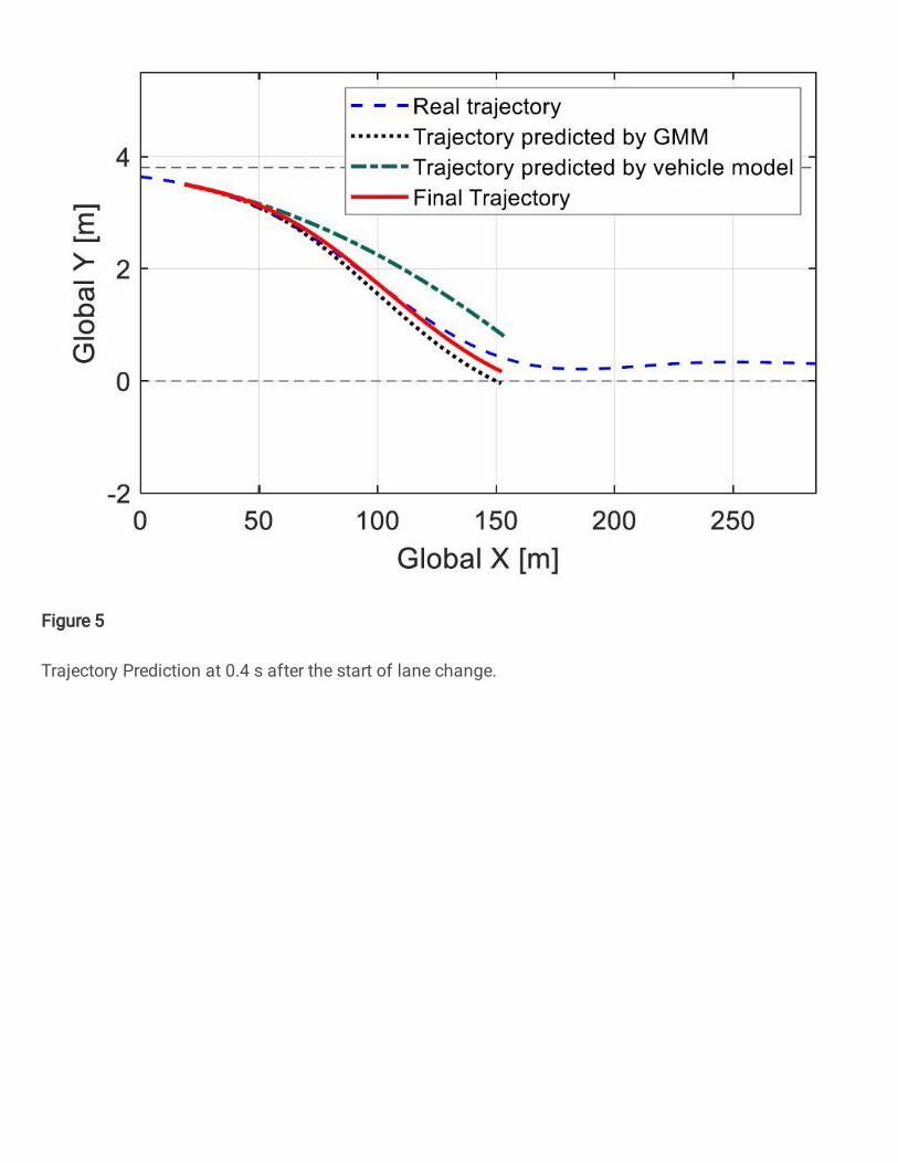
Figure 5

Trajectory Prediction at 0.4 s after the start of lane change.

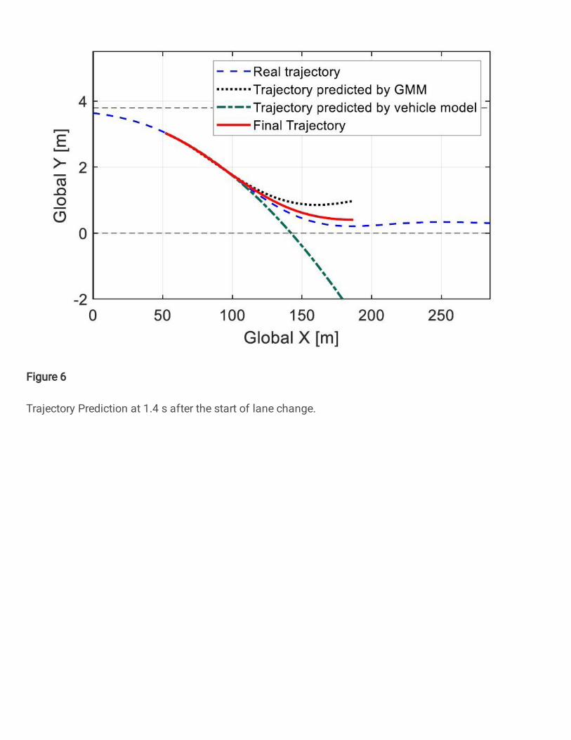
Figure 6

Trajectory Prediction at 1.4 s after the start of lane change.

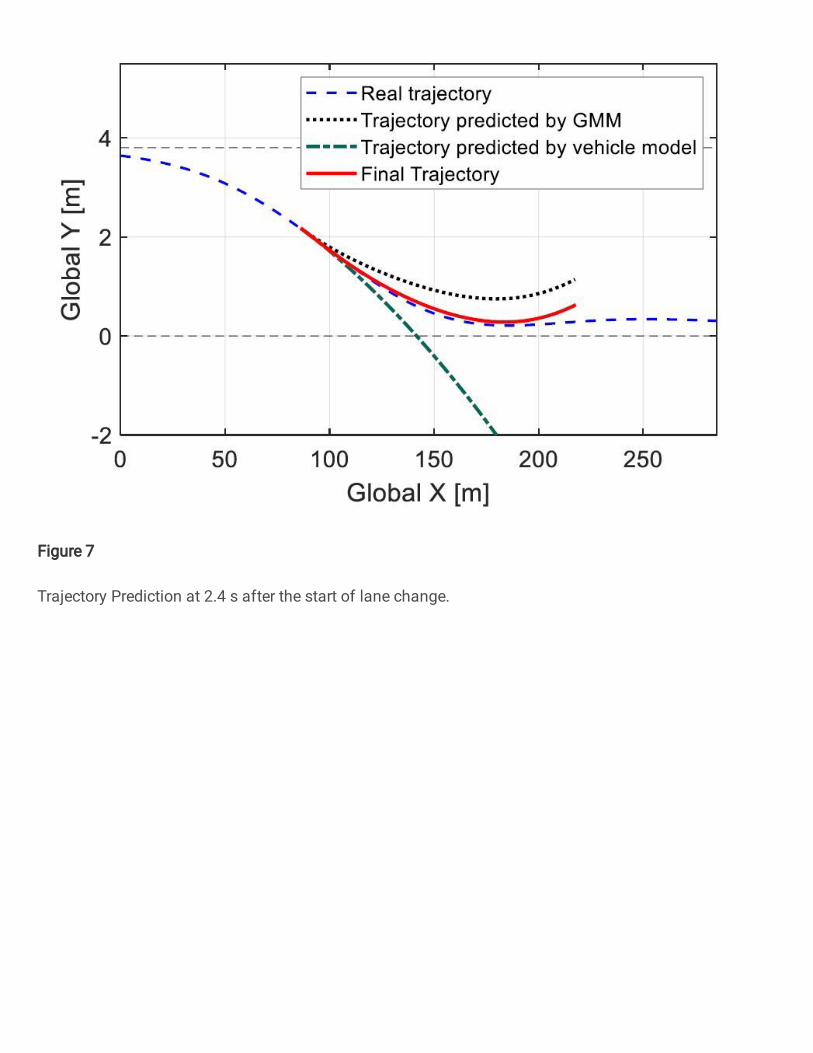
Figure 7

Trajectory Prediction at 2.4 s after the start of lane change.

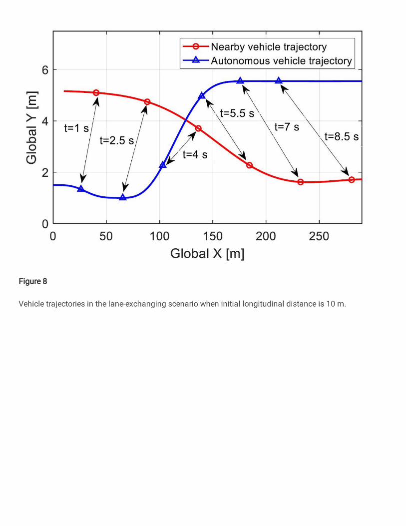
Figure 8

Vehicle trajectories in the lane-exchanging scenario when initial longitudinal distance is 10 m.

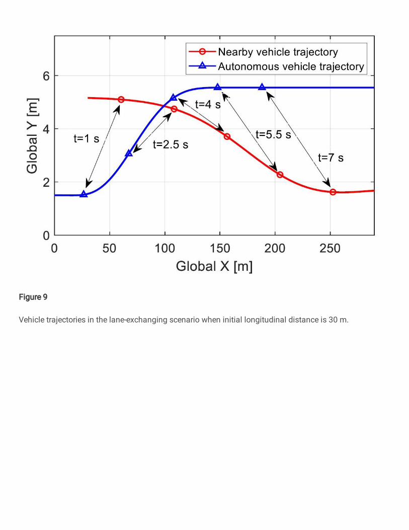
Figure 9

Vehicle trajectories in the lane-exchanging scenario when initial longitudinal distance is 30 m.

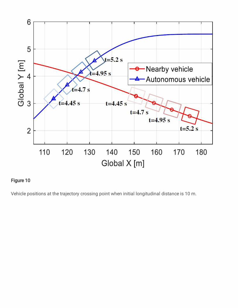
Figure 10

Vehicle positions at the trajectory crossing point when initial longitudinal distance is 10 m.

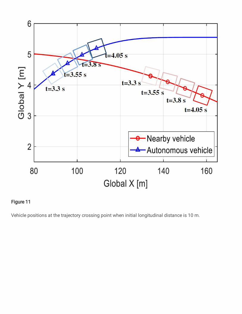
Figure 11

Vehicle positions at the trajectory crossing point when initial longitudinal distance is 10 m.

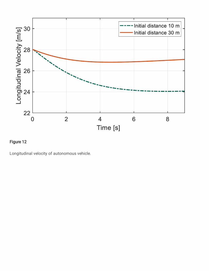
Figure 12

Longitudinal velocity of autonomous vehicle.

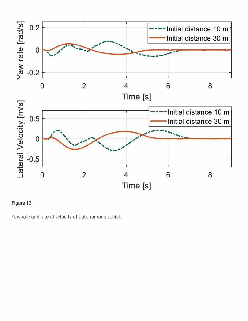
Figure 13

Yaw rate and lateral velocity of autonomous vehicle.