Embed Size (px)
Citation preview
Landslide Hazard in the Elk River Basin, Humboldt County, California
Prepared for North Coast Regional Water Quality Control Board
Santa Rosa, California
Prepared by Stillwater Sciences Arcata, California
1 June 2007
FINAL REPORT Landslide Hazard in the Elk River Basin Humboldt County, California
1 June 2007 Stillwater Sciences
i
Acknowledgements
The project benefited greatly from the following technical advisors who offered helpful discussion, guidance, and review of methods, model application, and model testing: Bill Dietrich (UC Berkeley, Department of Earth and Planetary Sciences), Bill Haneberg (Hanneberg Geoscience), Joshua Roering and Ben Mackey (University of Oregon, Department of Geological Sciences), Laura Vaugois (Washington Dept. of Natural Resources), and David Lamphear. Freshwater Creek Project Contractors Danny Hagens, Bill Weaver, and Eileen Weppner (Pacific Watershed Associates); and Drew Lewis (Sanborn Mapping) provided access to information and offered insightful discussion during the methodology workshop. Pacific Lumber Company graciously provided data and anecdotal information for the Elk River basin through coordination with Kate Sullivan, Amod Dhakal, John Ozwald, and Adrian Miller. Tom Hofweber and Chinmaya Lewis (Humboldt County Planning Department) and Sam Morrison (Bureau of Land Management) also provided access to essential data. The project would not have been possible without the interest and cooperation of these individuals and the organizations they represent. Suggested citation: Stillwater Sciences. 2007. Landslide Hazard in the Elk River Basin, Humboldt County, California. Final report. Prepared by Stillwater Sciences, Arcata, California for the North Coast Regional Water Quality Control Board.
FINAL REPORT Landslide Hazard in the Elk River Basin Humboldt County, California
1 June 2007 Stillwater Sciences
ii
Table of Contents
1 INTRODUCTION............................................................................................................1 1.1 Goals and objectives....................................................................................................... 2 1.2 Project Area .................................................................................................................... 2
1.2.1 Geologic setting..................................................................................................... 4 1.2.2 Climate .................................................................................................................. 4 1.2.3 Forest management history ................................................................................... 4 1.2.4 Sediment sources................................................................................................... 5
1.3 Overview of Approach and Products.............................................................................. 6
2 METHODS .......................................................................................................................8 2.1 Geomorphic Terrains...................................................................................................... 8
2.1.1 Geology ................................................................................................................. 8 2.1.2 Hillslope and channel gradient ............................................................................ 10 2.1.3 Cover type and stand age..................................................................................... 11
2.2 Pilot Basins................................................................................................................... 11 2.3 Modeling Landslide Hazards........................................................................................ 14
2.3.1 DEM development .............................................................................................. 14 2.3.2 Shallow landslide models.................................................................................... 17 2.3.3 Deep-seated landslide models ............................................................................. 23
2.4 Model Testing............................................................................................................... 25 2.4.1 Shallow landslide model testing.......................................................................... 25 2.4.2 Deep-seated landslide modeling.......................................................................... 32
3 RESULTS........................................................................................................................33 3.1 Shallow Landslide Modeling Results ........................................................................... 33 3.2 Shallow Landslide Model Testing................................................................................ 33
3.2.1 Model performance based on p-tests................................................................... 33 3.2.2 Model performance based on landslide density .................................................. 38 3.2.3 Correct landslide prediction versus area predicted to be unstable....................... 39
3.3 Deep-Seated Landslide Modeling Results.................................................................... 43
4 LANDSLIDE HAZARDS IN THE ELK RIVER BASIN...........................................44 4.1 Uses and Limitations .................................................................................................... 45 4.2 Future Analyses ............................................................................................................ 45
5 LITERATURE CITED..................................................................................................47
FINAL REPORT Landslide Hazard in the Elk River Basin Humboldt County, California
1 June 2007 Stillwater Sciences
i
Tables Table 1-1. Subwatersheds in the Elk River basin. .......................................................................... 3 Table 1-2. Sediment Budgets developed for North Fork and South Fork Elk rivers. .................... 6 Table 2-1. Terrain attributes in the Elk River Basin....................................................................... 9 Table 2-2. Summary of terrain characteristics in pilot subwatersheds. ........................................ 13 Table 2-3. LIDAR acquisition parameters. .................................................................................. 14 Table 2-4. Comparison of SHALSTAB potential instability in pilot area based on TIN vs krig
grids. ........................................................................................................................... 15 Table 2-5. Summary of parameter values used in SHALSTAB.V............................................... 19 Table 2-6. Summary of parameter constants used in predicting soil depth.................................. 20 Table 2-7. Summary of parameter values used in PISA............................................................... 22 Table 2-8. Existing landslide data in the Elk River basin. ........................................................... 31 Table 3-1. Percent of shallow landslides where P-test results were less than 0.5. ....................... 35 Table 3-2. Comparative model performance in Qh-Qmts-Qrt terrain based on p-values relating
potential instability at landslide points to potential instability at random points........ 36 Table 3-3. Comparative model performance in Qtwu terrain based on p-values relating potential
instability at landslide points to potential instability at random points. ..................... 37 Table 3-4. Comparative model performance in Ty terrain based on p-values relating potential
instability at landslide points to potential instability at random points. ..................... 38 Table 3-5. Summary of validation results: cumulative percent of area and cumulative percent of
landslides by instability class...................................................................................... 40 Table 3-6. Confidence intervals for threshold values and associated cumulative fraction of slides
or area classified by the threshold value..................................................................... 42 Table 3-7. Descriptive statistics for deep-seated landslide and ridge-and-valley signatures. ...... 43 Figures Figure 1-1. Elk River basin and subwatersheds. Figure 1-2. Annual average harvest rate for available photo periods in North Fork Elk River Figure 1-3. Annual harvest acreage for North Fork Elk River (all ownerships) as expressed in
clear-cut equivalent acres. Figure 1-4. Percent of watershed harvest annually for North Fork Elk River (all ownerships) as
expressed in clear-cut equivalent acres. Figure 1-5. Annual harvest acreage for South Fork Elk River (all ownerships) as expressed in
clear-cut equivalent acres. Figure 1-6. Percent of watershed harvest annually for South Fork Elk River (all ownerships) as
expressed in clear-cut equivalent acres. Figure 2-1. Geology in the Elk River basin. Figure 2-2. Hillslope gradient in the Elk River basin. Figure 2-3. Cover type in the Elk River basin. Figure 2-4. Stand age in portions of the Elk River basin. Figure 2-5. Pilot subwatersheds. Figure 2-6. Comparison of hillshade images from 1-m grids created from TINing and Kriging
methods. Figure 2-7. Elevation differences between 1-m grids created by TINing and Kriging methods. Figure 2-8. Tiling artifacts from the initial 1-m grid created by kriging. Figure 2-9. Comparison of curvature and elevation changes for different DEM grid sizes. Figure 2-10. Comparison of contours generated from different DEM grid sizes and methods. Figure 2-11. Composite shallow landslide data for model testing in the Elk River basin. Figure 3-1. SHALSTAB results in the Elk River basin.
FINAL REPORT Landslide Hazard in the Elk River Basin Humboldt County, California
1 June 2007 Stillwater Sciences
ii
Figure 3-2. SHALSTAB.V results in the Elk River basin. Figure 3-3. PISA results in the Elk River basin. Figure 3-4. PISA.V results in the Elk River basin. Figure 3-5. Density of landslides and random points by log (q/T) class from SHALSTAB. Figure 3-6. Density of landslides and random points by log (q/T) class from SHALSTAB.V. Figure 3-7. Density of landslides and random points by probability of sliding from PISA. Figure 3-8. Density of landslides and random points by probability of sliding from PISA.V. Figure 3-9. Cumulative percent of watershed area in instability classes. Figure 3-10. Cumulative percent of landslides in instability classes. Figure 3-11. Cumulative percent of watershed area as a function of the cumulative percent of the
number of landslides. Figure 3-12. DSLED-Rough results in the Elk River basin. Figure 3-13. DSLED-Drain results in the Elk River basin. Appendices Appendix A. Probability density functions for hillslope gradient at landslide points in different
geologic terrains. Appendix B. Model values at landslide initiation points. Appendix C. P-test Results at landslide initiation points based on random points. Appendix D. P-test Results at landslide initiation points based on points randomly sampled from
a probability distribution of unstable slopes. Appendix E. Results from sampling approach to determining landslide hazard threshold based on
model values at landslides and random points.
FINAL REPORT Landslide Hazard in the Elk River Basin Humboldt County, California
1 June 2007 Stillwater Sciences
1
1 INTRODUCTION
The Elk River watershed is listed as an impaired water body under Section 303(d) of the Clean Water Act. Water quality problems cited under the listing include sedimentation, threat of sedimentation, impaired quality of irrigation water, impaired quality of domestic water supply, impaired spawning habitat, increased rate and depth of flooding due to sediment, and property damage. Erosion, sediment discharge, and sedimentation has significantly modified the channel conditions of Elk River and its tributaries such that a threat to public health, safety, and property is present from increased incidences and magnitude of routine flooding, constituting a nuisance condition according to the Porter-Cologne Water Quality Control Plan. A program has been developed to recover waterbodies listed under 303(d) of the Clean Water Act via the establishment of Total Maximum Daily Loads (TMDL). The North Coast Regional Water Quality Control Board (NCRWQCB) has begun the process of establishing a TMDL for sediment in the Elk River watershed, with the goal of restoring and maintaining the sediment impaired beneficial uses of water of Elk River and its tributaries. The North Coast Regional Water Quality Control Board retained the team of Stillwater Sciences, Vestra, and Curry Group to evaluate landslide hazards in the Elk River basin as one component of TMDL development. Shallow landslides (both road-related and non-road-related) are acknowledged as the most common type of mass movement and dominant management-related sediment source impairing beneficial uses in Elk River (PWA 1998, PALCO 2004a, PALCO 2004b). Consequently, there is an immediate need for objective and repeatable methods that can be used in combination with existing terrain mapping, landslide inventories, and site-specific geotechnical slope stability assessments to reliably predict potential landslide hazards and identify land management activities compatible with recovery of sediment impaired beneficial uses. Such tools are ideally suited for use with additional information about sediment delivery and vulnerability of receptors to sediment impairment in assessing risk as part of the Elk River sediment TMDL analysis and implementation. Landslide hazard assessment can be broadly grouped into three main approaches: inferential, statistical, and mechanistic or physically-based (Dietrich et al. 2001, National Research Council 2004, Sidle and Ochiai 2006). The inferential approach utilizes remote sensing imagery, topographic and geologic mapping, geomorphic information (e.g., surface materials and landforms), historical information, and field observations to generate maps of landslide features and their relative activity. The approach requires knowledge of local geomorphic processes and professional judgment. Consequently, the reliability of the results are dependent on a map-maker’s skills and relevant experience. Although rooted in field observation, the process lacks objectivity and emphasizes where landslides have occurred rather than where there is potential for landslides to occur in the future. The statistical approach consists of inventorying all parameters related to landslide occurrence and subsequently conducting bivariate or multivariate statistical analyses to determine their relative importance. The process is more objective, but weighting of factors based on local experience introduces subjectivity and results are difficult to extrapolate beyond specific areas of study (Sidle and Ochiai 2006). Mechanistic or physically-based approaches use quantitative, process-based slope stability and shallow subsurface flow theories to predict the spatial distribution of relative slope stability (e.g., Hammond et al. 1992, Wu and Sidle 1995, Dietrich et al. 1995, Pack and Tarboton 1997, Dietrich and Montgomery 1998, Dhakal and Sidle 2003, Haneberg 2004). These approaches are more objective and have evolved rapidly with improved technologies for characterizing fine scale topography over large areas (e.g., LiDAR).
FINAL REPORT Landslide Hazard in the Elk River Basin Humboldt County, California
1 June 2007 Stillwater Sciences
2
These models, however, typically require spatially and temporally distributed model parameters (e.g., soil cohesion, root cohesion, soil bulk density, water table level, friction angle, soil depth, and hillslope gradient) and are highly simplified due to difficulty in characterizing parameter variability over large areas. Distributed, physically-based modeling approaches that predict the spatial distribution of relative slope stability from process-based models of slope stability and shallow subsurface flow using high-resolution digital topography take two general forms: probabilistic and deterministic (Haneberg 2000). Probabilistic approaches allow for uncertainty by assigning probability distributions to model parameters, while deterministic approaches establish invariant or spatially explicit parameter values and lack an element of uncertainty.
1.1 Goals and objectives
Both deterministic and probabilistic physically-based modeling approaches are used in this study to predict potential landslide hazards in the Elk River basin. The specific objectives of the work include the following:
1. Develop a database of observed shallow and deep-seated landslides, 2. Predict potentially unstable areas using grid-based deterministic and probabilistic hillslope
stability models, and 3. Objectively test model predictions of potential instability by relating predicted instability to
observed landslide occurrence.
1.2 Project Area
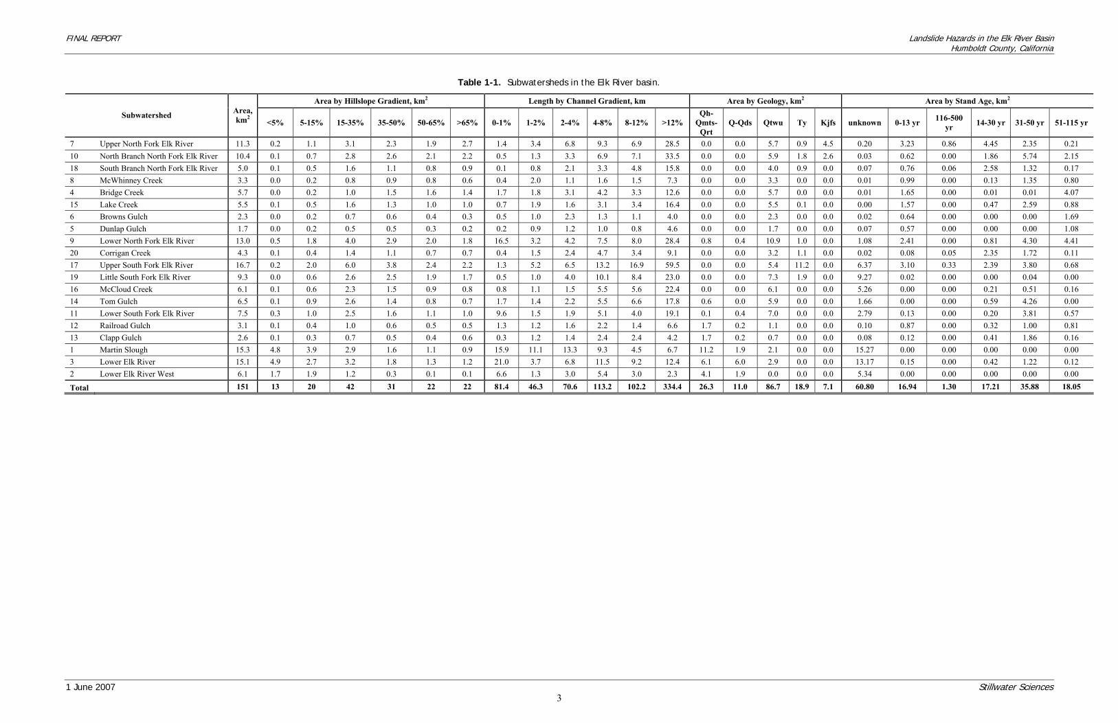
The Elk River basin (151 km2) is located south and east of the city of Eureka in Humboldt County, California (Figure 1-1, Table 1-1). The Elk River basin originates from the seaward slope of the outer Coast Range and flows westward across the coastal plain into Humboldt Bay. The basin can be divided into four main areas: (1) North Fork Elk River (58.2 km2), (2) South Fork (50.4 km2), (3) the lower Elk River downstream of the North Fork and South Fork confluence (26.9 km2), and (4) Martin Slough (15.3 km2). The majority of the North Fork Elk River basin is privately managed for industrial timber harvest, with private residential properties occupying only the lower 2%. The majority of the South Fork Elk River basin is also privately managed for industrial timber operations (65%), but 30% of the basin occurs within the Headwaters Forest Reserve (transferred to and managed by Bureau of Land Management since the 1999 Headwaters Deal) and the remaining 5% is private residential property in the lower South Fork Elk River valley. Lower Elk River is comprised of mixed private ownership, with approximately 24% zoned for timber production. Martin Slough is in mixed private ownership and includes urban development in the southeast portion of the City of Eureka.
FINAL REPORT Landslide Hazards in the Elk River Basin Humboldt County, California
1 June 2007 Stillwater Sciences
3
Table 1-1. Subwatersheds in the Elk River basin.
Area by Hillslope Gradient, km2 Length by Channel Gradient, km Area by Geology, km2 Area by Stand Age, km2
Subwatershed Area, km2 <5% 5-15% 15-35% 35-50% 50-65% >65% 0-1% 1-2% 2-4% 4-8% 8-12% >12%
Qh-Qmts-
Qrt Q-Qds Qtwu Ty Kjfs unknown 0-13 yr 116-500
yr 14-30 yr 31-50 yr 51-115 yr
7 Upper North Fork Elk River 11.3 0.2 1.1 3.1 2.3 1.9 2.7 1.4 3.4 6.8 9.3 6.9 28.5 0.0 0.0 5.7 0.9 4.5 0.20 3.23 0.86 4.45 2.35 0.21 10 North Branch North Fork Elk River 10.4 0.1 0.7 2.8 2.6 2.1 2.2 0.5 1.3 3.3 6.9 7.1 33.5 0.0 0.0 5.9 1.8 2.6 0.03 0.62 0.00 1.86 5.74 2.15 18 South Branch North Fork Elk River 5.0 0.1 0.5 1.6 1.1 0.8 0.9 0.1 0.8 2.1 3.3 4.8 15.8 0.0 0.0 4.0 0.9 0.0 0.07 0.76 0.06 2.58 1.32 0.17 8 McWhinney Creek 3.3 0.0 0.2 0.8 0.9 0.8 0.6 0.4 2.0 1.1 1.6 1.5 7.3 0.0 0.0 3.3 0.0 0.0 0.01 0.99 0.00 0.13 1.35 0.80 4 Bridge Creek 5.7 0.0 0.2 1.0 1.5 1.6 1.4 1.7 1.8 3.1 4.2 3.3 12.6 0.0 0.0 5.7 0.0 0.0 0.01 1.65 0.00 0.01 0.01 4.07 15 Lake Creek 5.5 0.1 0.5 1.6 1.3 1.0 1.0 0.7 1.9 1.6 3.1 3.4 16.4 0.0 0.0 5.5 0.1 0.0 0.00 1.57 0.00 0.47 2.59 0.88 6 Browns Gulch 2.3 0.0 0.2 0.7 0.6 0.4 0.3 0.5 1.0 2.3 1.3 1.1 4.0 0.0 0.0 2.3 0.0 0.0 0.02 0.64 0.00 0.00 0.00 1.69 5 Dunlap Gulch 1.7 0.0 0.2 0.5 0.5 0.3 0.2 0.2 0.9 1.2 1.0 0.8 4.6 0.0 0.0 1.7 0.0 0.0 0.07 0.57 0.00 0.00 0.00 1.08 9 Lower North Fork Elk River 13.0 0.5 1.8 4.0 2.9 2.0 1.8 16.5 3.2 4.2 7.5 8.0 28.4 0.8 0.4 10.9 1.0 0.0 1.08 2.41 0.00 0.81 4.30 4.41 20 Corrigan Creek 4.3 0.1 0.4 1.4 1.1 0.7 0.7 0.4 1.5 2.4 4.7 3.4 9.1 0.0 0.0 3.2 1.1 0.0 0.02 0.08 0.05 2.35 1.72 0.11 17 Upper South Fork Elk River 16.7 0.2 2.0 6.0 3.8 2.4 2.2 1.3 5.2 6.5 13.2 16.9 59.5 0.0 0.0 5.4 11.2 0.0 6.37 3.10 0.33 2.39 3.80 0.68 19 Little South Fork Elk River 9.3 0.0 0.6 2.6 2.5 1.9 1.7 0.5 1.0 4.0 10.1 8.4 23.0 0.0 0.0 7.3 1.9 0.0 9.27 0.02 0.00 0.00 0.04 0.00 16 McCloud Creek 6.1 0.1 0.6 2.3 1.5 0.9 0.8 0.8 1.1 1.5 5.5 5.6 22.4 0.0 0.0 6.1 0.0 0.0 5.26 0.00 0.00 0.21 0.51 0.16 14 Tom Gulch 6.5 0.1 0.9 2.6 1.4 0.8 0.7 1.7 1.4 2.2 5.5 6.6 17.8 0.6 0.0 5.9 0.0 0.0 1.66 0.00 0.00 0.59 4.26 0.00 11 Lower South Fork Elk River 7.5 0.3 1.0 2.5 1.6 1.1 1.0 9.6 1.5 1.9 5.1 4.0 19.1 0.1 0.4 7.0 0.0 0.0 2.79 0.13 0.00 0.20 3.81 0.57 12 Railroad Gulch 3.1 0.1 0.4 1.0 0.6 0.5 0.5 1.3 1.2 1.6 2.2 1.4 6.6 1.7 0.2 1.1 0.0 0.0 0.10 0.87 0.00 0.32 1.00 0.81 13 Clapp Gulch 2.6 0.1 0.3 0.7 0.5 0.4 0.6 0.3 1.2 1.4 2.4 2.4 4.2 1.7 0.2 0.7 0.0 0.0 0.08 0.12 0.00 0.41 1.86 0.16 1 Martin Slough 15.3 4.8 3.9 2.9 1.6 1.1 0.9 15.9 11.1 13.3 9.3 4.5 6.7 11.2 1.9 2.1 0.0 0.0 15.27 0.00 0.00 0.00 0.00 0.00 3 Lower Elk River 15.1 4.9 2.7 3.2 1.8 1.3 1.2 21.0 3.7 6.8 11.5 9.2 12.4 6.1 6.0 2.9 0.0 0.0 13.17 0.15 0.00 0.42 1.22 0.12 2 Lower Elk River West 6.1 1.7 1.9 1.2 0.3 0.1 0.1 6.6 1.3 3.0 5.4 3.0 2.3 4.1 1.9 0.0 0.0 0.0 5.34 0.00 0.00 0.00 0.00 0.00
Total 151 13 20 42 31 22 22 81.4 46.3 70.6 113.2 102.2 334.4 26.3 11.0 86.7 18.9 7.1 60.80 16.94 1.30 17.21 35.88 18.05
FINAL REPORT Landslide Hazards in the Elk River Basin Humboldt County, California
1 June 2007 Stillwater Sciences
4
1.2.1 Geologic setting
The Elk River basin is located along the southeastern margin of the actively uplifting and deforming southern Cascadia forearc basin at the leading edge of the northward migrating Mendocino triple junction. Northwest-trending faults and folds bound the dominant mountain ranges. The two basement units in the Project Area include the Franciscan Complex Central Belt – a Mesozoic to early Cenozoic age accretionary mélange enclosing blocks of more coherent sandstone, greenstone, and chert; and the Yager terrane – a Paleogene trench-slope deposit of thin-bedded argillite and sandstone turbidites with minor pebbly conglomerate (Ogle, 1953; McLaughlin et al., 2000, Marshall and Mendes 2005). The Wildcat Group, a thick transgressive-regressive sequence of marine siltstone and fine-grained sandstone of late Miocene to Pliocene age, rests unconformably on these basement units. Undifferentiated shallow water marine and fluvial deposits of middle to late Pleistocene age (Hookton Formation and related deposits) cap broad, accordant ridges across the western portions of the Elk River basin. These geologic terrains and the dominant hillslope geomorphic processes occurring within them are discussed in more detail in Section 2.1.1.
1.2.2 Climate
The Mediterranean climate of the Elk River basin is characterized by mild, wet winters and a prolonged summer dry season. Mean surface air temperature at the coast ranges from 9°C in January to 13°C in June, with summer temperature moderated by fog. Roughly 90% of the annual precipitation occurs as rainfall between October and April. Mean annual precipitation ranges from 99 cm at Eureka to 152 cm near Kneeland, located 20 km inland (elevation 810 m). Winter rainfall intensity and storm runoff are highly variable due to orographic lifting of moisture-laden, frontal air masses as they intersect the outer Coast Range. Storm events with rainfall intensity exceeding 3–4 inches a day are considered capable of initiating landslides (PALCO 2004b). A 24-hour rainfall total of 4–5 inches in the Eureka area (up to approximately 2000 ft) has an estimated return interval of 5 years (NOAA Atlas Vol XI Northern California cited in PALCO 2004b). Rainfall intensities exceeding 5 inches per day are rare and have only occurred 3 times between 1941 and 1998 (water years 1950, 1959, and 1997). The 24-hour rainfall total of 6.8 inches on December 27, 2002 set many records and caused widespread landslide damage and flooding. Annual peak discharges recorded at an Elk River gauge, located 0.3 km downstream of the North Fork Elk River and South Fork Elk River confluence, range from 23.4 m3s-1 to 112.2 m3s-1 for the period 1957–1967, 1997–1998. Estimated peak discharge for the 1.5-year flood at the Elk River gauge is 44.8 m3s-1 (Klein and Anderson, 1999).
1.2.3 Forest management history
The maritime coastal climate supports a coniferous lowland forest community dominated by redwood (Sequoia sempervirens), western hemlock (Tsuga heterophylla), Sitka spruce (Picea sitchensis), grand fir (Abies grandis), and Douglas-fir (Pseudotsuga menziesii). While large-scale harvest of these species has occurred in the Elk River watershed since the late 1800s, there has been a marked increase in harvest using clearcut silviculture in North Fork Elk River (Figures 1-2, 1-3, and 1-4) and South Fork Elk River (Figures 1-5 and 1-6) since 1994 (White, 2007). Harvest data for Lower Elk River and Martin Slough were not available at the time of this report.
FINAL REPORT Landslide Hazards in the Elk River Basin Humboldt County, California
1 June 2007 Stillwater Sciences
5
1.2.4 Sediment sources
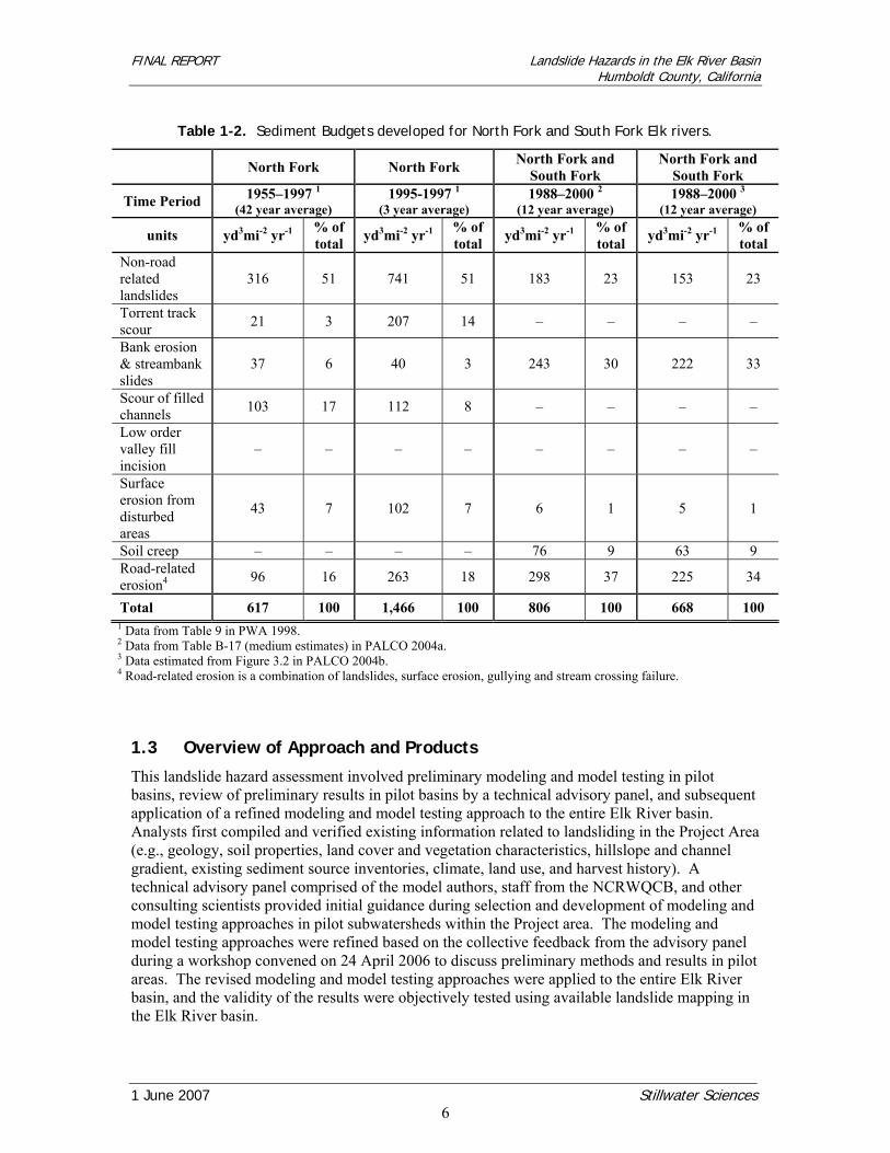
This landslide hazard assessment utilized landslide mapping and other related data collected during several prior studies focused on characterizing the rate and causes of sediment production and delivery in the Elk River basin. Pacific Watershed Associates (PWA) conducted a sediment source inventory in the North Fork Elk River basin in 1998 that identified sources of erosion and sediment delivery to stream channels, distinguished between natural and management-related sediment sources, and assessed opportunities for preventing and controlling future sediment sources (PWA 1998). The 1998 study involved extensive aerial photographic analysis and field inventory of erosion processes in the North Fork Elk River basin. PWA has conducted similar unpublished inventories for South Fork Elk River. A draft watershed analysis for the Elk River and Salmon Creek areas (PALCO 2004a), completed as a provision of PALCO’s Habitat Conservation Plan (PALCO 1999), included further analysis of mass wasting and surface erosion processes. Additional sediment source studies are ongoing in the watershed as part of the HCP agreement and cooperative projects with NCRWQCB (PALCO 2004b). Sediment budgets have been compiled by the Pacific Lumber Company for both North Fork and South Fork Elk rivers (Table 1-2). The majority of sediment delivered to the North Fork Elk River system originates from landslides. The main factors contributing to landslides and other management-related sediment supply in the Elk River basin are (PWA 1998, PALCO 1999, PALCO 2004a, PALCO 2004b):
• poorly located, constructed, or maintained roads; • logging with ground-based systems on steep slopes; • harvesting on inherently unstable slopes; • temporary reduction in root strength from clearcutting; and • legacy problems associated with old skid trails and abandoned roads.
FINAL REPORT Landslide Hazards in the Elk River Basin Humboldt County, California
1 June 2007 Stillwater Sciences
6
Table 1-2. Sediment Budgets developed for North Fork and South Fork Elk rivers.
North Fork North Fork North Fork and South Fork
North Fork and South Fork
Time Period 1955–1997 1 (42 year average)
1995-1997 1 (3 year average)
1988–2000 2 (12 year average)
1988–2000 3 (12 year average)
units yd3mi-2 yr-1 % of total yd3mi-2 yr-1 % of
total yd3mi-2 yr-1 % of total yd3mi-2 yr-1 % of
total Non-road related landslides
316 51 741 51 183 23 153 23
Torrent track scour 21 3 207 14 – – – –
Bank erosion & streambank slides
37 6 40 3 243 30 222 33
Scour of filled channels 103 17 112 8 – – – –
Low order valley fill incision
– – – – – – – –
Surface erosion from disturbed areas
43 7 102 7 6 1 5 1
Soil creep – – – – 76 9 63 9 Road-related erosion4 96 16 263 18 298 37 225 34
Total 617 100 1,466 100 806 100 668 100 1 Data from Table 9 in PWA 1998. 2 Data from Table B-17 (medium estimates) in PALCO 2004a. 3 Data estimated from Figure 3.2 in PALCO 2004b. 4 Road-related erosion is a combination of landslides, surface erosion, gullying and stream crossing failure.
1.3 Overview of Approach and Products
This landslide hazard assessment involved preliminary modeling and model testing in pilot basins, review of preliminary results in pilot basins by a technical advisory panel, and subsequent application of a refined modeling and model testing approach to the entire Elk River basin. Analysts first compiled and verified existing information related to landsliding in the Project Area (e.g., geology, soil properties, land cover and vegetation characteristics, hillslope and channel gradient, existing sediment source inventories, climate, land use, and harvest history). A technical advisory panel comprised of the model authors, staff from the NCRWQCB, and other consulting scientists provided initial guidance during selection and development of modeling and model testing approaches in pilot subwatersheds within the Project area. The modeling and model testing approaches were refined based on the collective feedback from the advisory panel during a workshop convened on 24 April 2006 to discuss preliminary methods and results in pilot areas. The revised modeling and model testing approaches were applied to the entire Elk River basin, and the validity of the results were objectively tested using available landslide mapping in the Elk River basin.

FINAL REPORT Landslide Hazards in the Elk River Basin Humboldt County, California
1 June 2007 Stillwater Sciences
7
The products of the landslide hazard assessment include the following:
• A data base of available terrain and landslide information for the Elk River basin; • 4-m digital elevation model (DEM) derived from LiDAR data and used as input for
hillslope stability modeling; • Grid-based results from individual models that predict potential shallow and deep-seated
instability; and • Results of validation tests used to evaluate and compare model performance.
FINAL REPORT Landslide Hazards in the Elk River Basin Humboldt County, California
1 June 2007 Stillwater Sciences
8
2 METHODS
2.1 Geomorphic Terrains
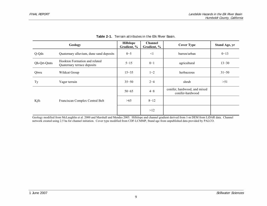
Evaluation of sediment production and transport potential at the watershed scale can be effectively organized by stratifying the watershed into geomorphic terrains. Four attributes were used to define geomorphic terrains in the Elk River Project Area based on their dominant role in determining and/or regulating erosion and transport processes: geology, hillslope gradient, channel gradient, and vegetation cover type (Table 2-1). Stand age classes were also defined for the Project area where records of forest management history were available. Other characteristics, such as local facies changes and strike and dip of geologic strata, yarding and silvicultural methods, and road construction and use are also important factors influencing slope instability, but are more difficult to characterize at the watershed scale. Geologic and stand age attributes were used in this study to (1) assign unique parameter values for hillslope stability modeling using PISA; (2) test the validity of model results for potential shallow instability; and (3) assess appropriate breaks in potential instability classes. Combining all four geomorphic terrain attributes provides the basis for conducting spatial analyses, extrapolating geomorphic processes and rates, and developing load management strategies during subsequent steps in the sediment TMDL process.
2.1.1 Geology
The Franciscan Complex Central Belt (Kjsf) comprises 4.7% of the Project Area, located exclusively in the Upper North Fork and North Branch North Fork subwatersheds, where it is in contact with the Yager terrane along the Freshwater fault (Figure 2-1). The Central belt Franciscan Complex is a late Jurassic to Cretaceous age accretionary mélange of meta-sandstone and meta-argillite enclosing blocks of more competent sandstone, greenstone, and chert. Large, deep-seated landslides and earthflows enclosing competent blocks are common in the Central belt Franciscan complex (Marshall and Mendes 2005). Blocks of competent sandstone commonly support steep slopes and weather to soils with low cohesion that are susceptible to debris slides and debris flows (Marshall and Mendes 2005).
FINAL REPORT Landslide Hazards in the Elk River Basin Humboldt County, California
1 June 2007 Stillwater Sciences
9
Table 2-1. Terrain attributes in the Elk River Basin.
Geology Hillslope Gradient, %
Channel Gradient, % Cover Type Stand Age, yr
Q-Qds Quaternary alluvium, dune sand deposits 0−5 <1 barren/urban 0−13
Qh-Qrt-Qmts Hookton Formation and related Quaternary terrace deposits 5−15 0−1 agricultural 13−30
Qtwu Wildcat Group 15−35 1−2 herbaceous 31−50
Ty Yager terrain 35−50 2−4 shrub >51
50−65 4−8 conifer, hardwood, and mixed conifer-hardwood
>65 8−12 Kjfs Franciscan Complex Central Belt
>12
Geology modified from McLaughlin et al. 2000 and Marshall and Mendes 2005. Hillslope and channel gradient derived from 1-m DEM from LiDAR data. Channel network created using 2.5 ha for channel initiation. Cover type modified from CDF-LCMMP, Stand age from unpublished data provided by PALCO.

FINAL REPORT Landslide Hazards in the Elk River Basin Humboldt County, California
1 June 2007 Stillwater Sciences
10
Yager terrane (Ty) of the Franciscan Complex Coastal Belt comprises 12.5% of the Project Area, located predominantly in the Upper South Fork, Upper North Fork, and North Branch North Fork watersheds (Figure 2-1). Yager terrane is a Paleogene trench-slope deposit that typically consists of highly folded and often sheared, dark gray argillite, sandstone, and conglomerate. In the North Fork Elk River, argillite (mudstones, siltstones, and shales) comprise 70% of the area; sandstones 25 %, and conglomerate less than 5% (PWA 1998). The sandstone facies is commonly a cliff-forming unit and exerts local base level control where streams have incised through younger, less resistant overlap deposits. The argillite facies is typically deeply weathered and sheared, promoting deep-seated flow failures on moderate slopes (Marshall and Mendes 2005). The Elk River Watershed analysis reports 2.5 shallow landslides per square kilometer in the Yager terrain over the period 1954−2000 (PALCO 2004a). The dominant geologic unit in the Elk River Basin is the Wildcat Group (Qtwu) (57.4% of the Project Area), a thick transgressive-regressive sequence of late Miocene to middle Quaternary marine and nonmarine overlap deposits that thins to the east (Ogle 1953, McCrory 1989, Clarke 1992). The Wildcat Group typically consists of poorly to moderately indurated siltstone and fine-grained silty sandstone that weathers to granular, non-cohesive, non-plastic clayey silts and clayey sands (Marshall and Mendes 2005). Wildcat Group terrain is characterized by steep and dissected topography sculpted by debris sliding, and is known for high historical erosion rates by shallow landsliding and debris flow. Shallow landslides in the Wildcat Group are commonly associated with headwall swales, inner gorges, and hollows where weathered soil and colluvium accumulate over relatively resistant, partially indurated, slowly permeable bedrock with bedding planes subparallel to the hillslope (PWA 1998). The Watershed Sensitivity Factor for bedrock geology (PALCO 1999) identifies the Wildcat Group as the most sensitive geology factor, and PWA (1998) reports that debris landslides from Wildcat terrain contribute 51% of the total sediment delivered to watercourses in the North Fork Elk River watershed. In the adjacent Freshwater Creek Watershed, 83% of all debris landslides are associated with siltstones comprising the Wildcat Group. The Elk River Watershed analysis reports 4.9 shallow landslides per square kilometer in Wildcat terrain over the period 1954−2000 (PALCO 2004a). Undifferentiated shallow water marine and fluvial deposits (gravel, sand, and silt) of the Hookton formation (Qh) cap broad, accordant ridge crests in the western part of the Elk River basin. These deposits and similar Quaternary marine terrace (Qmts) and Quaternary river terrace (Qrt) deposits comprised of poorly consolidated sand and gravel are prone to shallow landsliding on steep slopes and terrace risers. These deposits comprise 17.4% of the Project Area. The Elk River Watershed Analysis reports 9.9 shallow landslides per square kilometer in Hookton terrain over a 46-year period (1954−2000) (PALCO 2004a). Shallow landsliding and deep-seated bedding plane failures are common in Hookton terrain (Marshall and Mendes 2005).
2.1.2 Hillslope and channel gradient
Hillslope gradient is perhaps the most important factor controlling hillslope stability. For the purpose of stratifying the Project Areas into hillslope terrains meaningful to identification and management of landslide hazards, slope gradient was classified in 6 categories (0−5%, 5−15%, 15−35%, 35−50%, 50−65%, and >65%) based on values that have either been mandated in regulation or have emerged as practical thresholds (Table 2-1, Figure 2-2) (California Forest Practice Rules 2005, NMFS 2000, CGS 1997, Planwest Partners et al. 2005, PALCO 1999, PWA 1998). At a site scale, threshold slopes for instability may be strongly influenced by the
FINAL REPORT Landslide Hazards in the Elk River Basin Humboldt County, California
1 June 2007 Stillwater Sciences
11
geotechnical properties of the soil mantle and parent material; local surface and subsurface hydrology; and the type, age, and density of vegetation. Hillslope gradients in the Elk River basin were derived from a 1-m DEM generated from LiDAR data. Six channel gradient classes (<1%, 1–2%, 2–4%, 4–8%, 8–12, and >12%) were defined using 2-m DEM data from LiDAR and a 2.5 ha threshold for channel initiation (Table 2-1) (Buffleben, pers. comm., 19 December 2005). Gradient classes reflect characteristic channel morphologies, capacity for sediment transport, and potential for sediment storage (Montgomery and Buffington 1997, 1998). Channel gradient classes to do not integrate directly into analyses of landslide hazard, but are classified to inform subsequent TMDL analyses regarding potential for sediment delivery and transport.
2.1.3 Cover type and stand age
Vegetation cover reflects the relative potential for erosion due to differences in canopy cover, rainfall interception, and the effects of root distribution and strength on slope stability. Five vegetation cover types were defined in the Elk River Project Area: (1) mixed conifer-hardwood, (2) shrub, (3) herbaceous, (4) agricultural, and (5) urban and barren ground (Figure 2-3). These five categories were aggregated from vegetation data compiled as part of the Land Cover Mapping and Monitoring (LCMMP) program conducted by the USDA Forest Service Region 5 Remote Sensing Lab and the California Department of Forestry and Fire Protection's Fire and Resource Assessment Program (FRAP). Approximately 85% of the Elk River basin is mixed-conifer hardwood; the remainder is distributed evenly among herbaceous, agricultural, and urban cover types located predominantly in the lower watershed. Five stand age classes were defined using PALCO stand age data: <13 yr, 13−30 yr, 31−50 yr, and >51 yr (Figure 2-4, Table 1-1). At the time of this study, stand age data was available only for Pacific Lumber Company ownership (PALCO unpublished data). Stand age is used here to assign cohesive root strength parameters for modeling shallow landslide hazards using SHALSTAB.V, PISA, and PISA.V.
2.2 Pilot Basins
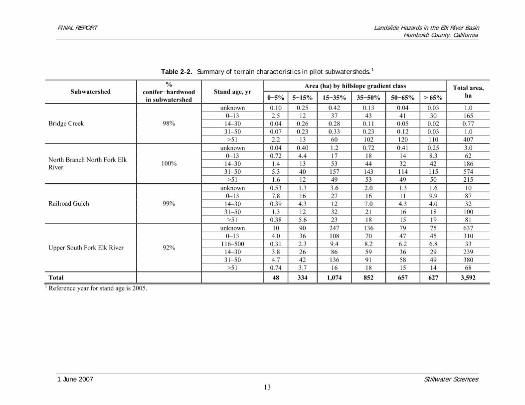
Four pilot subwatersheds were selected to conduct preliminary tests on optimal DEM grid size for modeling landslide hazards and to experiment with model parameters: Bridge Creek, Railroad Gulch, North Branch North Fork Elk, and Upper South Fork Elk (Figure 2-5, Table 2-2). Bridge Creek is comprised predominantly of relatively homogeneous bedrock of the Wildcat Group (Qtwu) that forms steep ridge and valley topography indicative of shallow debris slide and debris flow processes. Railroad Gulch is comprised of poorly consolidated gravel, sand, and silt deposits of the Hookton formation. North Branch North Fork Elk is one of only two basins where Franciscan Complex Central Belt (Kjfs) occurs over a large area. Topography is highly variable due to structural control by the Freshwater fault, the presence of highly sheared mélange units with a propensity for large deep-seated flow failure, and the occurrence of more resistant siltstone and sandstone units that form steep, ridge-and-valley topography. Upper South Fork Elk is comprised of eastward thinning Wildcat Group overlying Yager terrane. Planar, northeast-facing slopes parallel to bedding planes in Yager terrain exhibit deep-seated flow failure, while steeper south-facing slopes exhibit predominantly shallow landsliding.

FINAL REPORT Landslide Hazards in the Elk River Basin Humboldt County, California
1 June 2007 Stillwater Sciences
12
Each of the six hillslope stability models (SHALSTAB, SHALSTAB.V, PISA, PISA.V, DSLED-Rough, and DSLED-Drain) were applied in the pilot watersheds; mass wasting features were verified from existing landslide inventories using 2003 aerial photographs (scale 1:12,000) and DEM hillshade images; and preliminary tests were developed to validate and compare model results.
FINAL REPORT Landslide Hazards in the Elk River Basin Humboldt County, California
1 June 2007 Stillwater Sciences
13
Table 2-2. Summary of terrain characteristics in pilot subwatersheds.1
Area (ha) by hillslope gradient class Subwatershed
% conifer−hardwood in subwatershed
Stand age, yr 0−5% 5−15% 15−35% 35−50% 50−65% > 65%
Total area, ha
unknown 0.10 0.25 0.42 0.13 0.04 0.03 1.0 0–13 2.5 12 37 43 41 30 165
14–30 0.04 0.26 0.28 0.11 0.05 0.02 0.77 31–50 0.07 0.23 0.33 0.23 0.12 0.03 1.0
Bridge Creek 98%
>51 2.2 13 60 102 120 110 407 unknown 0.04 0.40 1.2 0.72 0.41 0.25 3.0
0–13 0.72 4.4 17 18 14 8.3 62 14–30 1.4 13 53 44 32 42 186 31–50 5.3 40 157 143 114 115 574
North Branch North Fork Elk River 100%
>51 1.6 12 49 53 49 50 215 unknown 0.53 1.3 3.6 2.0 1.3 1.6 10
0–13 7.8 16 27 16 11 9.9 87 14–30 0.39 4.3 12 7.0 4.3 4.0 32 31–50 1.3 12 32 21 16 18 100
Railroad Gulch 99%
>51 0.38 5.6 23 18 15 19 81 unknown 10 90 247 136 79 75 637
0–13 4.0 36 108 70 47 45 310 116–500 0.31 2.3 9.4 8.2 6.2 6.8 33 14–30 3.8 26 86 59 36 29 239 31–50 4.7 42 136 91 58 49 380
Upper South Fork Elk River 92%
>51 0.74 3.7 16 18 15 14 68 Total 48 334 1,074 852 657 627 3,592
1 Reference year for stand age is 2005.
FINAL REPORT Landslide Hazards in the Elk River Basin Humboldt County, California
1 June 2007 Stillwater Sciences
14
2.3 Modeling Landslide Hazards
The following sections describe methods used in modeling landslide hazards in the Elk River basin, including development of DEM topography from LiDAR data and application of models for predicting the location of shallow and deep-seated instability.
2.3.1 DEM development
2.3.1.1 LiDAR data
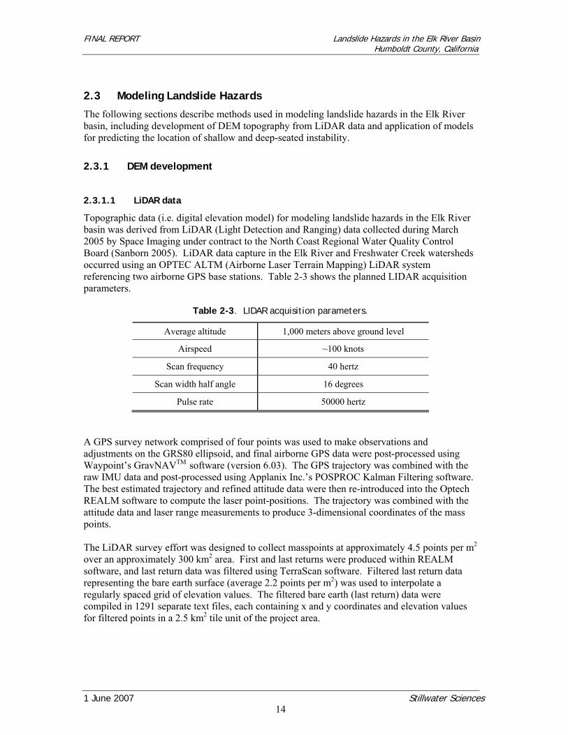
Topographic data (i.e. digital elevation model) for modeling landslide hazards in the Elk River basin was derived from LiDAR (Light Detection and Ranging) data collected during March 2005 by Space Imaging under contract to the North Coast Regional Water Quality Control Board (Sanborn 2005). LiDAR data capture in the Elk River and Freshwater Creek watersheds occurred using an OPTEC ALTM (Airborne Laser Terrain Mapping) LiDAR system referencing two airborne GPS base stations. Table 2-3 shows the planned LIDAR acquisition parameters.
Table 2-3. LIDAR acquisition parameters.
Average altitude 1,000 meters above ground level
Airspeed ~100 knots
Scan frequency 40 hertz
Scan width half angle 16 degrees
Pulse rate 50000 hertz
A GPS survey network comprised of four points was used to make observations and adjustments on the GRS80 ellipsoid, and final airborne GPS data were post-processed using Waypoint’s GravNAVTM software (version 6.03). The GPS trajectory was combined with the raw IMU data and post-processed using Applanix Inc.’s POSPROC Kalman Filtering software. The best estimated trajectory and refined attitude data were then re-introduced into the Optech REALM software to compute the laser point-positions. The trajectory was combined with the attitude data and laser range measurements to produce 3-dimensional coordinates of the mass points. The LiDAR survey effort was designed to collect masspoints at approximately 4.5 points per m2 over an approximately 300 km2 area. First and last returns were produced within REALM software, and last return data was filtered using TerraScan software. Filtered last return data representing the bare earth surface (average 2.2 points per m2) was used to interpolate a regularly spaced grid of elevation values. The filtered bare earth (last return) data were compiled in 1291 separate text files, each containing x and y coordinates and elevation values for filtered points in a 2.5 km2 tile unit of the project area.
FINAL REPORT Landslide Hazards in the Elk River Basin Humboldt County, California
1 June 2007 Stillwater Sciences
15
2.3.1.2 DEM generation
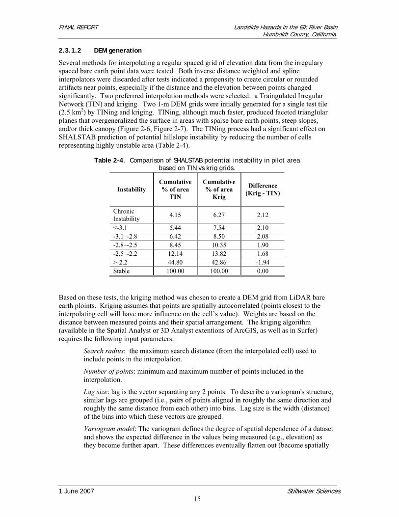
Several methods for interpolating a regular spaced grid of elevation data from the irregulary spaced bare earth point data were tested. Both inverse distance weighted and spline interpolators were discarded after tests indicated a propensity to create circular or rounded artifacts near points, especially if the distance and the elevation between points changed significantly. Two preferrred interpolation methods were selected: a Traingulated Irregular Network (TIN) and kriging. Two 1-m DEM grids were intially generated for a single test tile (2.5 km2) by TINing and kriging. TINing, although much faster, produced faceted trianglular planes that overgeneralized the surface in areas with sparse bare earth points, steep slopes, and/or thick canopy (Figure 2-6, Figure 2-7). The TINing process had a significant effect on SHALSTAB prediction of potential hillslope instability by reducing the number of cells representing highly unstable area (Table 2-4).
Table 2-4. Comparison of SHALSTAB potential instability in pilot area
based on TIN vs krig grids.
Instability Cumulative % of area
TIN
Cumulative % of area
Krig
Difference (Krig - TIN)
Chronic Instability 4.15 6.27 2.12
<-3.1 5.44 7.54 2.10 -3.1–-2.8 6.42 8.50 2.08 -2.8–-2.5 8.45 10.35 1.90 -2.5–-2.2 12.14 13.82 1.68 >-2.2 44.80 42.86 -1.94 Stable 100.00 100.00 0.00
Based on these tests, the kriging method was chosen to create a DEM grid from LiDAR bare earth ploints. Kriging assumes that points are spatially autocorrelated (points closest to the interpolating cell will have more influence on the cell’s value). Weights are based on the distance between measured points and their spatial arrangement. The kriging algorithm (available in the Spatial Analyst or 3D Analyst extentions of ArcGIS, as well as in Surfer) requires the following input parameters:
Search radius: the maximum search distance (from the interpolated cell) used to include points in the interpolation.
Number of points: minimum and maximum number of points included in the interpolation.
Lag size: lag is the vector separating any 2 points. To describe a variogram's structure, similar lags are grouped (i.e., pairs of points aligned in roughly the same direction and roughly the same distance from each other) into bins. Lag size is the width (distance) of the bins into which these vectors are grouped.
Variogram model: The variogram defines the degree of spatial dependence of a dataset and shows the expected difference in the values being measured (e.g., elevation) as they become further apart. These differences eventually flatten out (become spatially
FINAL REPORT Landslide Hazards in the Elk River Basin Humboldt County, California
1 June 2007 Stillwater Sciences
16
independent), and the distance to where the curve first flattens out is known as the range. The linear model defines a straight line from 0 until the range.
In creating a DEM surface from bare earth points, slope angles and roughness should faithfully represent the actual landscape in order to accurately characterize potential instability. Specifiying a small number of points and small search radius minimizes computation time and generates a rougher surface over small length scales; whereas specifying a large number of points and a wide radius substantially increases computation time and leads to a smoother surface. A 1-m grid from kriging was initially created for the Project Area from bare earth LiDAR points using a spherical semivariogram, search radius of 20 m, and maximum of 16 points (Sanborn 2005). Hillslope stability models were run in four pilot areas using this 1-m grid. Elevation anomolies over small length scales (e.g., ground artifacts such as stumps, fallen logs, and vegetative piles) created topographic “noise” (small scale roughness) in the 1-m grid that led to a wide distribution of high potential instability in isolated grid cells. In addition, tiling artifacts were apparent in shaded relief, flow accumulation, hillslope gradient, and curvature plots (Figure 2-8). Several approaches were tested in pilot areas to objectively smooth topographic noise from the 1-m grid, including a second order local polynomial interpolator and a soil production model (refer to Section 2.3.2.1 for description of the model). The second order local polynomial interpolator resulted in significant artifacts. The soil production and transport model, an approach to estimating spatially distributed soil depth as part of the SHALSTAB.V model (refer to Section 2.3.2.2), effectively removed most elevation anomolies but excessively smoothed the landscape to the point that high potential instability was concentrated exclusively in steep swales and low order channels. After testing various smoothing techniques, kriging was used on LiDAR bare earth points in a pilot area to create different size DEM grids (2m, 3m, 4m and 5m). Comparison of curvature and elevation differences with respect to the 1m grid (Figure 2-9) and contour patterns from the various grid sizes (Figure 2-10) suggested that the 4-m grid was optimal for modeling hillslope stability in the Project Area because it (1) substantially reduced variance in curvature over short length scales while minimizing elevation change relative to the 1-m grid, (2) maintained the definition of unchanneled valleys apparent in 5-m contours, and (3) reduced computation time required for model application and other spatial analyses. To create the final 4-m DEM used in modeling hillslope stability in the Project Area, grids were recreated from the 1291 tiles using the kriging algorithm (linear variogram, radius of 200 m, and maximum of 64 points). To minimize tiling artifacts, tile boundaries were first buffered by 100 m, and points within buffers on adjacent tiles were combined. Point shapefiles were exported to text files and read into Surfer (the kriging algorithm ran faster in Surfer than in ArcGIS). Output grids from Surfer were then mosaiced in ArcGIS. To further minimize tiling artifacts, each buffered grid was first clipped to the coordinates of the corners of each tile, and the clipped grid tiles were mosaiced together into a single 4m grid for the Elk River basin. Minor tiling artifacts were still apparent in the 4-m DEM after creating the final 4-m DEM mosaic.
FINAL REPORT Landslide Hazards in the Elk River Basin Humboldt County, California
1 June 2007 Stillwater Sciences
17
2.3.2 Shallow landslide models
Two distributed, physically-based models were initially selected for predicting potential shallow landslide hazards based on their common usage and past performance in forested mountainous terrain: the deterministic model SHALSTAB (Montgomery and Dietrich 1994, Dietrich et al. 2001) and the probabilistic model PISA (Haneberg 2004, 2005). Two variations of these models were subsequently included in the analyses to allow more parameterization, most notably, spatially variation in soil depth. These include SHALSTAB.V (Dietrich et al. 1995), and what we refer to here as PISA.V. All four approaches are objective, mechanistic models based on high resolution (4-m) DEM topography developed from LiDAR data. 2.3.2.1 SHALSTAB
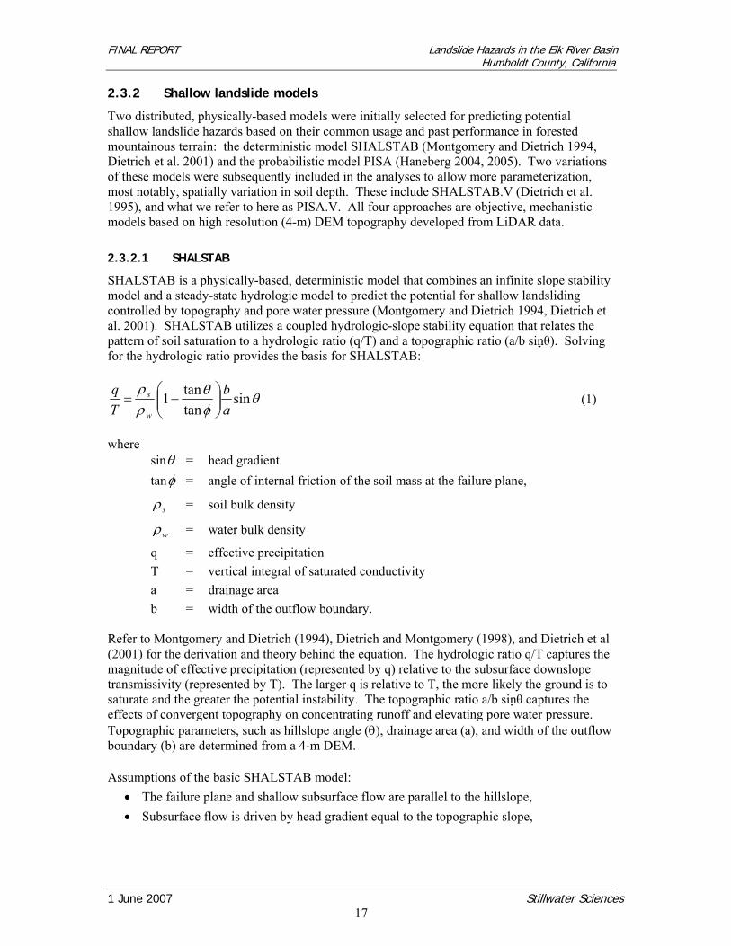
SHALSTAB is a physically-based, deterministic model that combines an infinite slope stability model and a steady-state hydrologic model to predict the potential for shallow landsliding controlled by topography and pore water pressure (Montgomery and Dietrich 1994, Dietrich et al. 2001). SHALSTAB utilizes a coupled hydrologic-slope stability equation that relates the pattern of soil saturation to a hydrologic ratio (q/T) and a topographic ratio (a/b sinθ). Solving for the hydrologic ratio provides the basis for SHALSTAB:
θφθ
ρρ
sintantan1
ab
Tq
w
s⎟⎟⎠
⎞⎜⎜⎝
⎛−= (1)
where
sinθ = head gradient tanφ = angle of internal friction of the soil mass at the failure plane,
sρ = soil bulk density
wρ = water bulk density
q = effective precipitation T = vertical integral of saturated conductivity a = drainage area b = width of the outflow boundary.
Refer to Montgomery and Dietrich (1994), Dietrich and Montgomery (1998), and Dietrich et al (2001) for the derivation and theory behind the equation. The hydrologic ratio q/T captures the magnitude of effective precipitation (represented by q) relative to the subsurface downslope transmissivity (represented by T). The larger q is relative to T, the more likely the ground is to saturate and the greater the potential instability. The topographic ratio a/b sinθ captures the effects of convergent topography on concentrating runoff and elevating pore water pressure. Topographic parameters, such as hillslope angle (θ), drainage area (a), and width of the outflow boundary (b) are determined from a 4-m DEM. Assumptions of the basic SHALSTAB model:
• The failure plane and shallow subsurface flow are parallel to the hillslope, • Subsurface flow is driven by head gradient equal to the topographic slope,
FINAL REPORT Landslide Hazards in the Elk River Basin Humboldt County, California
1 June 2007 Stillwater Sciences
18
• Soils are cohesionless, • Root strength is neglected (although root strength strongly effects slope stability, it is
highly variable over small spatial and termporal scales and difficult to quantify), and • Unit weights of saturated and unsaturated soil are equal.
Soil bulk density and the angle of internal friction are treated as spatially constant. Soil bulk density is set at 1,700 kg m-3 (saturated bulk density typically lies between about 1,700 and 2,000 kg m-3). The angle of internal friction is set at a relatively high value of 45 degrees, in part, to compensate for the absence of root strength. This basic version of SHALSTAB has been shown to reliably delineate areas prone to shallow landsliding in parts of the Coast Ranges of northern California, Oregon, and Washington (Montgomery et al. 1998, Shaw and Vaugeois 1999, Dietrich et al. 2001). The model does not predict the location of deep-seated instability nor instability associated with steep, planar slopes typical of inner gorges. The model and documentation for use with ArcView is available from the University of California Berkeley at http://socrates.berkeley.edu/~geomorph/shalstab/index.htm. 2.3.2.2 SHALSTAB.V
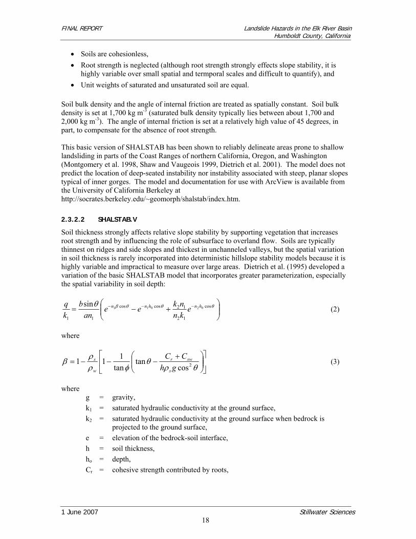
Soil thickness strongly affects relative slope stability by supporting vegetation that increases root strength and by influencing the role of subsurface to overland flow. Soils are typically thinnest on ridges and side slopes and thickest in unchanneled valleys, but the spatial variation in soil thickness is rarely incorporated into deterministic hillslope stability models because it is highly variable and impractical to measure over large areas. Dietrich et al. (1995) developed a variation of the basic SHALSTAB model that incorporates greater parameterization, especially the spatial variability in soil depth:
⎟⎟⎠
⎞⎜⎜⎝
⎛+−= −−− θθθβθ cos
12
12coscos
11
02011sin hnhnn e
knnkee
anb
kq
(2)
where
⎥⎦
⎤⎢⎣
⎡⎟⎟⎠
⎞⎜⎜⎝
⎛ +−−−=
θρθ
φρρβ 2cos
tantan
111gh
CC
s
swr
w
s (3)
where
g = gravity, k1 = saturated hydraulic conductivity at the ground surface, k2 = saturated hydraulic conductivity at the ground surface when bedrock is
projected to the ground surface, e = elevation of the bedrock-soil interface, h = soil thickness, ho = depth, Cr = cohesive strength contributed by roots,
FINAL REPORT Landslide Hazards in the Elk River Basin Humboldt County, California
1 June 2007 Stillwater Sciences
19
Csw = cohesive strength of soil when wet. n1 and n2 are exponents describing the decrease in hydraulic conductivity normal to the ground surface,
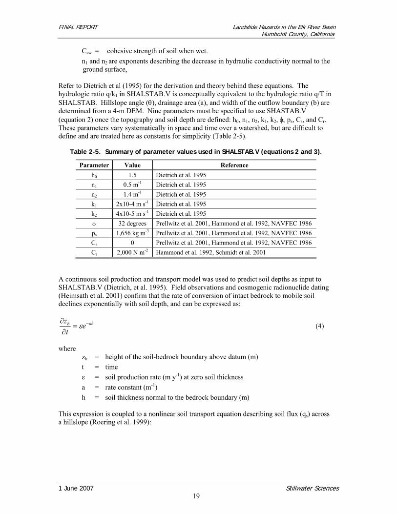
Refer to Dietrich et al (1995) for the derivation and theory behind these equations. The hydrologic ratio q/k1 in SHALSTAB.V is conceptually equivalent to the hydrologic ratio q/T in SHALSTAB. Hillslope angle (θ), drainage area (a), and width of the outflow boundary (b) are determined from a 4-m DEM. Nine parameters must be specified to use SHASTAB.V (equation 2) once the topography and soil depth are defined: h0, n1, n2, k1, k2, φ, ps, Cs, and Cr. These parameters vary systematically in space and time over a watershed, but are difficult to define and are treated here as constants for simplicity (Table 2-5).
Table 2-5. Summary of parameter values used in SHALSTAB.V (equations 2 and 3).
Parameter Value Reference h0 1.5 Dietrich et al. 1995 n1 0.5 m-1 Dietrich et al. 1995 n2 1.4 m-1 Dietrich et al. 1995 k1 2x10⁻⁴ m s-1 Dietrich et al. 1995 k2 4x10⁻⁵ m s-1 Dietrich et al. 1995 φ 32 degrees Prellwitz et al. 2001, Hammond et al. 1992, NAVFEC 1986 ps 1,656 kg m-3 Prellwitz et al. 2001, Hammond et al. 1992, NAVFEC 1986 Cs 0 Prellwitz et al. 2001, Hammond et al. 1992, NAVFEC 1986 Cr 2,000 N m-2 Hammond et al. 1992, Schmidt et al. 2001
A continuous soil production and transport model was used to predict soil depths as input to SHALSTAB.V (Dietrich, et al. 1995). Field observations and cosmogenic radionuclide dating (Heimsath et al. 2001) confirm that the rate of conversion of intact bedrock to mobile soil declines exponentially with soil depth, and can be expressed as:
ahb etz −=∂∂ ε (4)
where
zb = height of the soil-bedrock boundary above datum (m) t = time ε = soil production rate (m y-1) at zero soil thickness a = rate constant (m-1) h = soil thickness normal to the bedrock boundary (m)
This expression is coupled to a nonlinear soil transport equation describing soil flux (qs) across a hillslope (Roering et al. 1999):
FINAL REPORT Landslide Hazards in the Elk River Basin Humboldt County, California
1 June 2007 Stillwater Sciences
20
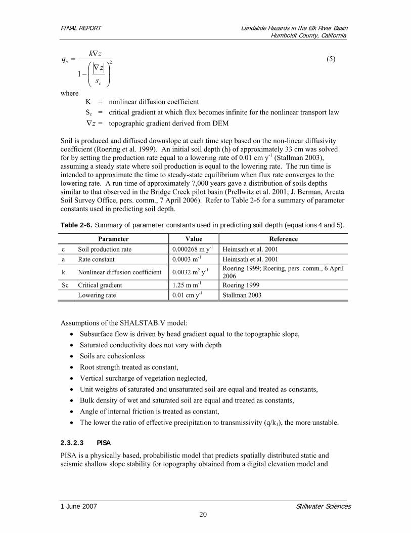
2
1 ⎟⎟⎠
⎞⎜⎜⎝
⎛ ∇−
∇=
c
s
sz
zkq (5)
where K = nonlinear diffusion coefficient Sc = critical gradient at which flux becomes infinite for the nonlinear transport law z∇ = topographic gradient derived from DEM Soil is produced and diffused downslope at each time step based on the non-linear diffusivity coefficient (Roering et al. 1999). An initial soil depth (h) of approximately 33 cm was solved for by setting the production rate equal to a lowering rate of 0.01 cm y-1 (Stallman 2003), assuming a steady state where soil production is equal to the lowering rate. The run time is intended to approximate the time to steady-state equilibrium when flux rate converges to the lowering rate. A run time of approximately 7,000 years gave a distribution of soils depths similar to that observed in the Bridge Creek pilot basin (Prellwitz et al. 2001; J. Berman, Arcata Soil Survey Office, pers. comm., 7 April 2006). Refer to Table 2-6 for a summary of parameter constants used in predicting soil depth. Table 2-6. Summary of parameter constants used in predicting soil depth (equations 4 and 5).
Parameter Value Reference ε Soil production rate 0.000268 m y-1 Heimsath et al. 2001 a Rate constant 0.0003 m-1 Heimsath et al. 2001
k Nonlinear diffusion coefficient 0.0032 m2 y-1 Roering 1999; Roering, pers. comm., 6 April 2006
Sc Critical gradient 1.25 m m-1 Roering 1999 Lowering rate 0.01 cm y-1 Stallman 2003 Assumptions of the SHALSTAB.V model:
• Subsurface flow is driven by head gradient equal to the topographic slope, • Saturated conductivity does not vary with depth • Soils are cohesionless • Root strength treated as constant, • Vertical surcharge of vegetation neglected, • Unit weights of saturated and unsaturated soil are equal and treated as constants, • Bulk density of wet and saturated soil are equal and treated as constants, • Angle of internal friction is treated as constant, • The lower the ratio of effective precipitation to transmissivity (q/k1), the more unstable.
2.3.2.3 PISA
PISA is a physically based, probabilistic model that predicts spatially distributed static and seismic shallow slope stability for topography obtained from a digital elevation model and
FINAL REPORT Landslide Hazards in the Elk River Basin Humboldt County, California
1 June 2007 Stillwater Sciences
21
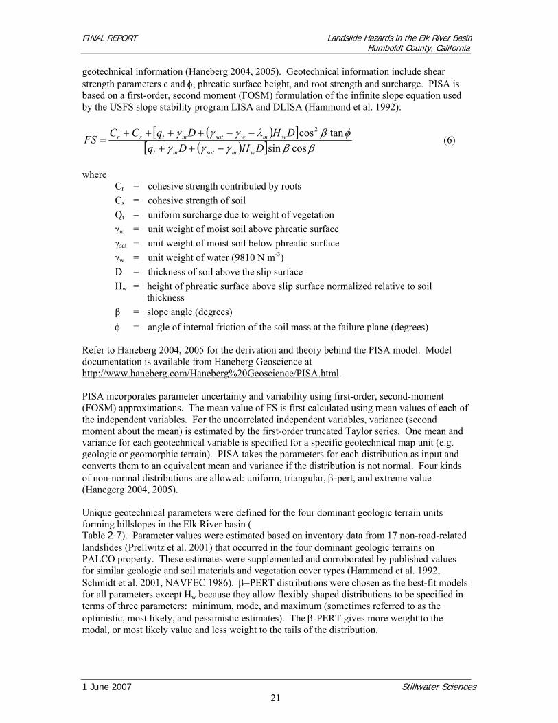
geotechnical information (Haneberg 2004, 2005). Geotechnical information include shear strength parameters c and φ, phreatic surface height, and root strength and surcharge. PISA is based on a first-order, second moment (FOSM) formulation of the infinite slope equation used by the USFS slope stability program LISA and DLISA (Hammond et al. 1992):
( )[ ]( )[ ] ββγγγ
φβλγγγcossin
tancos2
DHDqDHDqCCFS
wmsatmt
wmwsatmtsr
−++−−++++
= (6)
where
Cr = cohesive strength contributed by roots Cs = cohesive strength of soil Qt = uniform surcharge due to weight of vegetation γm = unit weight of moist soil above phreatic surface γsat = unit weight of moist soil below phreatic surface γw = unit weight of water (9810 N m-3) D = thickness of soil above the slip surface Hw = height of phreatic surface above slip surface normalized relative to soil
thickness β = slope angle (degrees) φ = angle of internal friction of the soil mass at the failure plane (degrees)
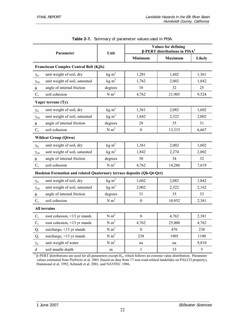
Refer to Haneberg 2004, 2005 for the derivation and theory behind the PISA model. Model documentation is available from Haneberg Geoscience at http://www.haneberg.com/Haneberg%20Geoscience/PISA.html. PISA incorporates parameter uncertainty and variability using first-order, second-moment (FOSM) approximations. The mean value of FS is first calculated using mean values of each of the independent variables. For the uncorrelated independent variables, variance (second moment about the mean) is estimated by the first-order truncated Taylor series. One mean and variance for each geotechnical variable is specified for a specific geotechnical map unit (e.g. geologic or geomorphic terrain). PISA takes the parameters for each distribution as input and converts them to an equivalent mean and variance if the distribution is not normal. Four kinds of non-normal distributions are allowed: uniform, triangular, β-pert, and extreme value (Hanegerg 2004, 2005). Unique geotechnical parameters were defined for the four dominant geologic terrain units forming hillslopes in the Elk River basin ( Table 2-7). Parameter values were estimated based on inventory data from 17 non-road-related landslides (Prellwitz et al. 2001) that occurred in the four dominant geologic terrains on PALCO property. These estimates were supplemented and corroborated by published values for similar geologic and soil materials and vegetation cover types (Hammond et al. 1992, Schmidt et al. 2001, NAVFEC 1986). β−PERT distributions were chosen as the best-fit models for all parameters except Hw because they allow flexibly shaped distributions to be specified in terms of three parameters: minimum, mode, and maximum (sometimes referred to as the optimistic, most likely, and pessimistic estimates). The β-PERT gives more weight to the modal, or most likely value and less weight to the tails of the distribution.
FINAL REPORT Landslide Hazards in the Elk River Basin Humboldt County, California
1 June 2007 Stillwater Sciences
22
Table 2-7. Summary of parameter values used in PISA.
Values for defining β-PERT distributions in PISA1 Parameter Unit
Minimum Maximum Likely
Franciscan Complex Central Belt (Kjfs)
γm unit weight of soil, dry kg m3 1,201 1,602 1,361
γsat unit weight of soil, saturated kg m3 1,762 2,002 1,842
φ angle of internal friction degrees 18 32 25
Cs soil cohesion N m2 4,762 21,905 9,524
Yager terrane (Ty)
γm unit weight of soil, dry kg m3 1,361 2,082 1,602
γsat unit weight of soil, saturated kg m3 1,842 2,322 2,002
φ angle of internal friction degrees 28 35 31
Cs soil cohesion N m2 0 13,333 6,667
Wildcat Group (Qtwu)
γm unit weight of soil, dry kg m3 1,361 2,002 1,602
γsat unit weight of soil, saturated kg m3 1,842 2,274 2,002
φ angle of internal friction degrees 30 34 32
Cs soil cohesion N m2 4,762 14,286 7,619
Hookton Formation and related Quaternary terrace deposits (Qh-Qt-Qrt)
γm unit weight of soil, dry kg m3 1,602 2,082 1,842
γsat unit weight of soil, saturated kg m3 2,002 2,322 2,162
φ angle of internal friction degrees 31 35 33
Cs soil cohesion N m2 0 10,952 2,381
All terrains
Cr root cohesion, <13 yr stands N m2 0 4,762 2,381
Cr root cohesion, >13 yr stands N m2 4,762 25,000 4,762
Qt surcharge, <13 yr stands N m2 0 476 238
Qt surcharge, >13 yr stands N m2 238 1905 1190
γw unit weight of water N m2 na na 9,810
d soil mantle depth m 1 13 5 1 β-PERT distributions are used for all parameters except Hw, which follows an extreme value distribution. Parameter
values estimated from Prellwitz et al. 2001 (based on data from 17 non-road-related landslides on PALCO property), Hammond et al. 1992, Schmidt et al. 2001, and NAVFEC 1986.
FINAL REPORT Landslide Hazards in the Elk River Basin Humboldt County, California
1 June 2007 Stillwater Sciences
23
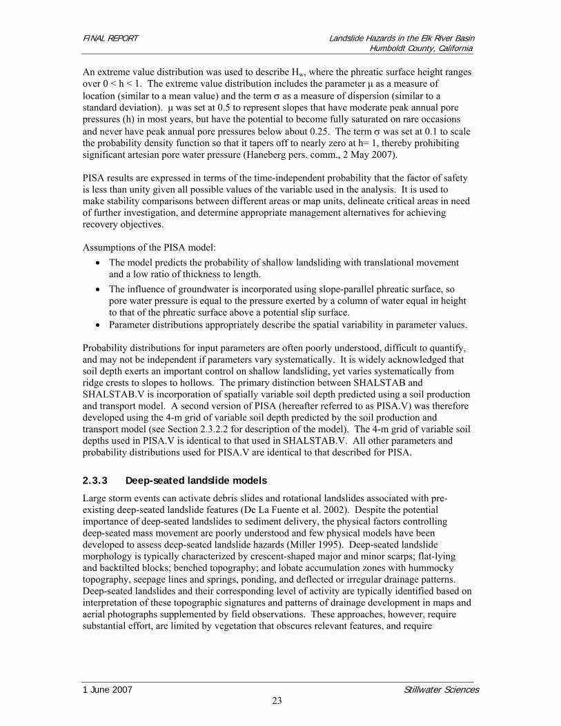
An extreme value distribution was used to describe Hw, where the phreatic surface height ranges over 0 < h < 1. The extreme value distribution includes the parameter µ as a measure of location (similar to a mean value) and the term σ as a measure of dispersion (similar to a standard deviation). µ was set at 0.5 to represent slopes that have moderate peak annual pore pressures (h) in most years, but have the potential to become fully saturated on rare occasions and never have peak annual pore pressures below about 0.25. The term σ was set at 0.1 to scale the probability density function so that it tapers off to nearly zero at h= 1, thereby prohibiting significant artesian pore water pressure (Haneberg pers. comm., 2 May 2007). PISA results are expressed in terms of the time-independent probability that the factor of safety is less than unity given all possible values of the variable used in the analysis. It is used to make stability comparisons between different areas or map units, delineate critical areas in need of further investigation, and determine appropriate management alternatives for achieving recovery objectives. Assumptions of the PISA model:
• The model predicts the probability of shallow landsliding with translational movement and a low ratio of thickness to length.
• The influence of groundwater is incorporated using slope-parallel phreatic surface, so pore water pressure is equal to the pressure exerted by a column of water equal in height to that of the phreatic surface above a potential slip surface.
• Parameter distributions appropriately describe the spatial variability in parameter values. Probability distributions for input parameters are often poorly understood, difficult to quantify, and may not be independent if parameters vary systematically. It is widely acknowledged that soil depth exerts an important control on shallow landsliding, yet varies systematically from ridge crests to slopes to hollows. The primary distinction between SHALSTAB and SHALSTAB.V is incorporation of spatially variable soil depth predicted using a soil production and transport model. A second version of PISA (hereafter referred to as PISA.V) was therefore developed using the 4-m grid of variable soil depth predicted by the soil production and transport model (see Section 2.3.2.2 for description of the model). The 4-m grid of variable soil depths used in PISA.V is identical to that used in SHALSTAB.V. All other parameters and probability distributions used for PISA.V are identical to that described for PISA.
2.3.3 Deep-seated landslide models
Large storm events can activate debris slides and rotational landslides associated with pre-existing deep-seated landslide features (De La Fuente et al. 2002). Despite the potential importance of deep-seated landslides to sediment delivery, the physical factors controlling deep-seated mass movement are poorly understood and few physical models have been developed to assess deep-seated landslide hazards (Miller 1995). Deep-seated landslide morphology is typically characterized by crescent-shaped major and minor scarps; flat-lying and backtilted blocks; benched topography; and lobate accumulation zones with hummocky topography, seepage lines and springs, ponding, and deflected or irregular drainage patterns. Deep-seated landslides and their corresponding level of activity are typically identified based on interpretation of these topographic signatures and patterns of drainage development in maps and aerial photographs supplemented by field observations. These approaches, however, require substantial effort, are limited by vegetation that obscures relevant features, and require
FINAL REPORT Landslide Hazards in the Elk River Basin Humboldt County, California
1 June 2007 Stillwater Sciences
24
professional judgment based on experience with the local geology and topography; resulting in hazard mapping that is subjective. A suite of tools for objective delineation of terrain prone to deep-seated landslides and earthflows using high-resolution digital topographic data is currently being developed (McKean and Roering 2004, Roering et al. 2005, Mackey et al. 2005, Mackey et al. 2006, Roering et al. 2006). These deep-seated landslide and earthflow detection (DSLED) algorithms identify terrain that has already experienced deep-seated slope instability, and thus has a higher potential for reactivation (Roering et al. 2006). The methods provide predictive power in identifying slide-prone terrain, and are best utilized as reconnaissance tools in combination with aerial photographic interpretation and field mapping. The models are being developed and tested at sites in the northern California Coast Range, Western Cascade Range of Oregon, and elsewhere (Roering et al. 2006); and have been used to successfully identify deep-seated mass movement associated with the Franciscan melange in the nearby Eel River basin (Mackey et al. 2005, Mackey et al. 2006). Two of the three DSLED algorithms, DSLED Rough and DSLED Drain, are used to identify surface roughness and drainage patterns associated with potential deep-seated mass movement in the Elk River basin. 2.3.3.1 DSLED-Rough
DLSED-Rough uses the eigenvalue ratio of cell-normal vector dispersion to identify local terrain roughness from airborne LiDAR topographic data (McKean and Roering 2004, Roering et al. 2006). The approach is based on observations that landslide surfaces are commonly rougher (on a local scale of a few meters) than adjacent unfailed slopes. DSLED Rough is used to construct unit vectors perpendicular to each cell in the DEM, and the statistical method of eigenvalue ratios (ln[S1/S2]) is used to describe the clustering of vector orientations (refer to McKean and Roering 2004 for the methods and theory behind eigenvalue ratios). The rougher the surface, the more divergent and less clustered the vector orientations. Mass movement and internal deformation of a deep-seated slide mass leads to rougher terrain with low ln (S1/S2) values relative to surrounding unfailed terrain. Eigenvalue ratios (ln [S1/S2]) in the Elk River basin were calculated in a 15x15 m circular sampling window that moves over the 1-m DEM. Ln (S1/S2) values were then spatially averaged using a circular moving window with a 50-m radius. The DSLED-Rough algorithm identifies terrace and floodplain areas as “rough” due to small-scale variations in aspect on relatively flat surfaces. To objectively remove these types of false positives and isolate signatures of potential deep-seated instability between ridges and valleys, the following portions of the watershed were filtered from the spatially averaged DSLED-Rough results:
1. Polygons mapped at a coarse scale as alluvium (Qal of McLaughlin et al. 2000, Q and Qds of Marshall and Mendes 2005) were adjusted to fit terrain slope (7−9%) and curvature signatures extracted from alluviated valley bottoms in the Project Area using a 1-m DEM grid;
2. In the NW section of Elk River basin only (Martin Slough, Lower Elk River, Lower Elk River West), a slope threshold of 9% was used to identify low gradient valley bottoms (not mapped as alluvium) and broad-crested ridges,
3. Watershed divides were buffered 20 m on each side, and 4. Channels were buffered on each side using the square of the Strahler order (e.g., 1-m
buffer for Strahler order 1 and 36-m buffer for Strahler order 6).
FINAL REPORT Landslide Hazards in the Elk River Basin Humboldt County, California
1 June 2007 Stillwater Sciences
25
2.3.3.2 DSLED-drain
DSLED-Drain uses spatially-averaged values of drainage area per unit contour width (a/b) calculated using high-resolution topographic data from airborne LiDAR to identify large, poorly-drained landforms commonly associated with deep-seated slope instability (Mackey et al. 2005, Mackey et al. 2006). Deep-seated mass movement typically affects hillslope hydrology by impeding channel incision and slowing drainage network development, leading to large areas with lower a/b values than surrounding unfailed terrain (Mackey et al. 2005, Mackey e l. 2006). DSLED-Drain calculates a/b values using the multiple-directional flow algorithm FD8 (Quinn et al. 1995, Costa-Cabral and Burgess 1994, Tarboton 1997). FD8 divides flow into each downstream neighboring cell based on the slope to that neighbor, while increasing the degree of flow convergence from the watershed divide to the channel head. The approach explicitly recognizes divergent flow on convex slopes and convergent flow on concave slopes and along valley bottoms. The catchment area, FD a/b, is the total drainage area for each cell divided by the cell width. FD a/b values were spatially averaged using a circular moving window with a 50-m radius. False positives associated with ridge crests and valley bottoms were filtered using the steps described above for DSLED-Rough.
2.4 Model Testing
2.4.1 Shallow landslide model testing
Hypothesis tests were developed to objectively validate model results and to evaluate the relative performance of the various modeling approaches. Validation tests and analyses of test results had the following primary objectives:
1. Evaluate the success of each model at correctly classifying potential instability at mapped shallow landslides in the Project Area,
2. Evaluate the aerial extent to which each model may over predict potential shallow instability in the Project Area;
3. Compare the relative performance of various modeling approaches; and 4. Determine appropriate thresholds for breaks in potential instability classes that balance
the goals of maximizing correct landslide prediction and minimizing over prediction of unstable area.
Different geologic terrains in the Elk River basin (refer Section 2.1 above for descriptions of geologic terrains) are dominated by different hillslope geomorphic processes and rates due to different parent materials, weathering processes and rates, slope angles, surface and subsurface hydrologic interactions, and drainage density. Validation tests were therefore, independently conducted in the four dominant geologic terrains in the Elk River basin: Hookton and similar Quaternary terrace deposits (Qh-Qt-Qrt), Wildcat group (Qtwu), Yager terrain (Ty), and Franciscan Complex Central Belt (Kjfs). Tests in difference geologic terrains were conducted with the goal of evaluating the extent to which model performance and model threshold values vary in different geologic terrains.
FINAL REPORT Landslide Hazards in the Elk River Basin Humboldt County, California
1 June 2007 Stillwater Sciences
26
2.4.1.1 Hypothesis testing
An objective and repeatable method of hypothesis testing was developed to address two basic questions:
1. Do shallow landslide models predict greater potential instability at known slide locations than at random positions in the landscape?
2. Are the models better predictors of instability than predictions based solely on hillslope gradient?
Two statistical tests were developed to address these questions, one based on randomly selected points (irrespective of slope), and the other accounting for the covariate hillslope gradient during the point selection process. For both tests, the null hypothesis states that model predictions of potential instability at randomly selected points in the Elk River basin will be greater than or equal to model predictions at a landslide point. For both tests, the alternative hypothesis states that model predictions of potential instability will be greater at slide points than at random points. A p-test value, indicating the extent to which models predict greater instability at random points than at a landslide point, was estimated as:
B
ZZp
j
B
ii
j
)(1
≥=
∑= ,
where Zi is the model value at the ith randomly selected point, Zj is the model value at the jth slide, and B is the number of randomly selected points (B=5,000); (Zi ≥ Zj) is 1 if true and 0 if false (≥ defined here as greater instability). P-values vary from 0 to 1; with a value of 0 indicating a test where predicted instability is always greater at a slide than at random points, and a value of 1 indicating a test where predicted instability is always greater at random points than at a slide. A p-value <0.5 indicates that the model predicts greater instability at a landslide than at more than half of the 5,000 random points. The percentage of p-values <0.5 were summarized for each model validation test. Different threshold p-values can be selected to change the rigor of the test. To address the first question, model values for potential instability at mapped landslide points were tested against model values of potential instability at a set of random points (sampled with replacement) within the Elk River basin. Random sampling with replacement (i.e., the same point can be selected more than once) is used here because comparisons using model values for all 4-m grid cells in the Project Area were computationally unfeasible (e.g., the 4-m grid of model results includes over 9 million cells in the 151 km2 Project Area). The large number of randomly selected points (B=5,000) ensures that the sample is representative of the population of all points in the Project Area. Random sampling occurred using the “sample” function in the “R” statistical package (R Development Core Team 2006). To address the second question, model values for potential instability at mapped landslide points were tested against model values for potential instability at a set of random points sampled (with replacement) from a probability distribution of potentially unstable slopes defined by hillslope gradient at landslide points. By incorporating hillslope gradient as a covariate, the second test specifically evaluates whether the models are better predictors of
FINAL REPORT Landslide Hazards in the Elk River Basin Humboldt County, California
1 June 2007 Stillwater Sciences
27
instability than predictions based solely on hillslope gradient. Probability density functions for hillslope gradient were constructed for each geologic terrain using the mean and standard deviation of gradient values at all non-road-related landslide points mapped in that geologic terrain. Probability densities were calculated for all points in the landscape, assuming a normal distribution for hillslope gradient (a reasonable assumption based on graphical analyses of hillslope gradient values at landslide points). The probability densities were calculated using the “dnorm” function in the “R” statistical package. Unique probability distributions for gradient were developed for each terrain type (Appendix A). Probability densities for hillslope gradient at landslide points were then used to weight random sampling of points using the “sample” function in the “R” statistical package. The performance of landslide models in validation tests may be significantly influenced by uncertainties in the location of landslide initiation points due to inaccuracies in the original mapping of landslides on aerial photos (approximately 1:18000 scale) and on coarse-scale topographic maps (1:24,000 USGS quadrangles) during field observations. Due to uncertainty in the location of landslide initiation relative to mapped shallow landslide points, statistical tests were conducted at two spatial resolutions: (1) model values for potential instability at a landslide point, and (2) model values for the highest potential instability within a specified neighborhood of a landslide point. The first resolution assumes that shallow landslide points in the existing landslide database are indeed initiation points, landslide initiation points are accurately and precisely mapped within 4 meters (grid cell size), and that model predicted values at slide initiation points accurately reflect the limiting instability associated with failure. The second resolution allows for uncertainty in the spatial location of landslide initiation relative to the mapped landslide point by determining the model value with the highest (most limiting) potential instability within an 8-meter radius around a mapped landslide point. An 8-m radius considers the model results in all 4-m grid cells adjacent to the mapped landslide initiation point. 2.4.1.2 Correct landslide prediction versus area predicted to be unstable
The fraction of slides and random points within each geologic terrain was used to evaluate relationships between (1) the fraction of slides correctly classified and (2) the fraction of the Elk River basin predicted to be unstable. The analysis was intended to guide selection of model thresholds that consider both the extent to which a model correctly classifies mapped landslides as unstable and the potential over prediction of unstable areas. Cumulative relative frequency distributions were graphed by fitting smoothed logistic regression curves to the data (i.e., model predictions of potential instability, fraction of slides correctly classified, and fraction of area predicted to be unstable) using the “sm” library (Bowman and Azzalini 1997, 2005) within the “R” statistical package. A kernel smoothing technique was used to generate the curves representing the cumulative relative frequency functions using the “sm.binomial” function in the “R” statistical package. For each model type, two cumulative relative frequency functions were generated, one for the most unstable value within an 8 m radius of slide points (RS), and the other for the most unstable value within an 8 m radius of randomly selected points (RL). We defined RL(x) as the fraction of the Project Area within a particular terrain type for which the model predicted potential instability is greater than x, and RS(x) as the fraction of the slides within a particular terrain type for which model predicted potential instability is greater than x. RL(x) is estimated based on the large sample (5,000) of random points, and the random selection process ensures that this large sample is representative of the population of all points in the Project Area.
FINAL REPORT Landslide Hazards in the Elk River Basin Humboldt County, California
1 June 2007 Stillwater Sciences
28
2.4.1.3 Determination of potential instability thresholds
In selecting appropriate threshold model values for potential instability classes, there is a fundamental tradeoff between (1) the cost of incorrectly classifying landslides and (2) the cost of over predicting potentially unstable area. An instability threshold that incorrectly classifies a landslide location as stable may not adequately protect similar areas prone to landsliding. Conversely, overprediction of unstable area may result in unnecessary restrictions and associated site evaluation costs in stable and economically productive areas. A particularly useful threshold for managing landslide hazards can be defined as the potential instability value that simultaneously minimizes the total costs associated with incorrect slide classification and over prediction of potential instability. The total cost of incorrectly predicting slides as stable (more stable than threshold x) can be expressed as: A*(1-RS(x)), where A is the total cost associated with incorrectly classifying slides as stable in the Project Area. The total cost associated with over predicting unstable areas can be expressed as: B*(RL(x)-c), where B is the total cost due to over prediction in the Project Area, and c is the fraction of the landscape that is unstable (estimated by the number of slides over the number of cells in the landscape). The value of x that minimizes the total cost [A*(1-RS(x))+B*(RL(x)-c)] is the same value that maximizes A*RS(x)-B*RL(x). If the total cost associated with incorrectly classifying slides as stable is equal to the total cost due to over prediction (i.e., A=B), then the problem reduces to maximizing RS(x)-RL(x). In practice, the maximum value for RS(x)-RL(x) is found by calculating the difference between the two cumulative relative frequency functions for model predicted instability. To obtain an expected value and confidence interval for the threshold value based on this approach, the following steps were taken:
1. Bootstrap samples of model predicted potential instability within an 8 m radius of slides and model predicted instability within an 8 m radius of randomly selected points were generated;
2. Logistic regression curves were fit to data from both bootstrap samples by kernel smoothing (refer to methods described above);
3. A threshold value was calculated based on the method described above; 4. Steps 1−3 were repeated 5,000 times; 5. The expected value (i.e., calculated as the mean of all samples) and 95% confidence
interval for the threshold value (based on the 2.5 percentile and 97.5 percentile), along with the expected value and 95% confidence interval for the cumulative relative frequencies RS(x) and RL(x) associated with the threshold model value, were calculated.
2.4.1.4 Landslide density graphs
A second, independent method of evaluating model performance is to compare the landslide density (i.e., number of landslides counted in an instability class divided by the total area in that instability class) to the random point density in each instability class (Dietrich et al. 2001). Model performance can be objectively determined by significantly greater landslide density in increasingly unstable classes compared to the nearly constant density of random points across instability classes. If a model performs poorly, there would be little difference between the densities of landslides and random points. If model predicted instability strongly covaries with
FINAL REPORT Landslide Hazards in the Elk River Basin Humboldt County, California
1 June 2007 Stillwater Sciences
29
slope, the random point distribution may reflect the distribution of hillslope gradient in the basin.
Classes of model values were defined for Shalstab and Shalstab V and for PISA and PISA V; and three values were calculated for each class: 1) number of random points, 2) number of slide points, and 3) watershed area. For each class, point densities were calculated by dividing either the number of random points or the number of slide points by the watershed area. Densities are based on maximum instability within an 8 m radius of points. The number of random points in a given terrain was scaled to match the total number of landslide points by calculating the proportion of random points within each defined class and then multiplying these proportions by the total number of slide points. Relative densities in different instability classes are therefore, more important than the absolute density values.
2.4.1.5 Existing landslide inventories
Several independent sets of landslide data exist for the Elk River basin. These include: • a sediment source inventory initially prepared by Pacific Watershed Associates in 1998
for Pacific Lumber Company and subsequently updated by Pacific Watershed Associates in 2001 as part of Watershed Analysis;
• a forensic landslide investigation prepared by Pacific Lumber Company in 2003; • compilation of landslide mapping by Pacific Lumber Company in 2006; and • compilation of landslide mapping from review of timber harvest plans by the California
Geologic Survey in 2005. Table 2-8 summarizes the important attributes of existing landslide inventories relevant to testing the validity of shallow landslide model results in the Elk River basin. The 2001 inventory of landslides in the ElK River basin conducted by Pacific Watershed Associates for Pacific Lumber Company was undertaken as part of a sediment source inventory for Watershed Analysis (PALCO 2004a). The landslide inventory involved mapping landslide features and attributes from an historical aerial photographic time series (1954, 1966, 1974, 1987, 1994, 1997, and 2000). Over 850 shallow landslide initiation points were mapped from air photos and transferred onto base maps at a scale of 1:18,000. A sample of landslide features mapped from aerial photography were field verified during Watershed Analysis and during sediment source inventories on Pacific Lumber Company land prior to 1998 (PWA 1998). The landslide forensic investigation conducted by Pacific Lumber Company in 2003 supplemented the sediment source inventory by mapping 64 shallow landslides in the Elk River basin that were triggered by an intense rainfall event in December 2002 (PALCO unpublished data). The study also identified causal mechanisms for landslide initiation and estimated associated sediment delivery. Accepted field methods were used in the 2003 forensic study to document landslide type, morphology, and dimensions; geologic, geomorphologic, and hydrologic controls; soil shear strength parameters; volume of sediment production and delivery; vegetation characteristics; forest management and timber harvest associations; and road and stream crossing associations. The methods used in the 2003 forensic study were generally consistent and compatible with those used in the 2001 landslide inventory by PWA. Pacific Lumber Company provided Stillwater Sciences with a coverage and associated database of attributes that included landslide initiation points identified in the 2001 landslide inventory and 2003 forensic study, as well as landslide initiation points and polygons identified during
FINAL REPORT Landslide Hazards in the Elk River Basin Humboldt County, California
1 June 2007 Stillwater Sciences
30
more recent geologic investigations associated with THP development in pilot subwatersheds. The data base contained 1,144 shallow landslide initiation points in the Elk River basin. Mapping of erosion and depositional areas for individual shallow landslides was not available for the Project Area at the time of this study. These data are the most comprehensive and extensively ground-verified landslide data available for the Project Area. All shallow landslide initiation points from this compilation that were characterized as debris slides, translational slides, or translational debris slides and occurred on open slopes with no apparent road association were used in model validation tests (Figure 2-11). The California Geological Survey mapped landslides and their attributes from aerial photographs (1940 to 2000), compiled existing landslide mapping, and interpreted relative landslide potential in the Elk River basin during preparation of the Watershed Mapping Series for the Elk River Watershed (Marshall and Mendes 2005). Nearly 550 shallow landslide features were mapped from aerial photographs and classified following DMG (1997) and Cruden and Varnes (1996). Landslide data compiled by Marshall and Mendes (2005) were not used in model validation tests for the following reasons: (1) landslides were mapped and compiled at a coarse scale (1:24,000), (2) no landslide mapping was available for the period after 2000, (3) field verification of the mapping was limited, (4) the work included no assessment of positional accuracy, and (5) the data do not include an attribute for road association. CGS interpreted relative landslide potential in the Elk River basin based on a matrix of values assigned to various classes of (1) landslide feature type and activity level, (2) hillslope and channel gradient derived from 10-m DEM data, (3) potential instability predicted by SHALSTAB, and (4) geologic terrain type. Individual coverages were converted to grids, assigned values according to the matrix, and merged into final grid. The performance of landslide models in validation tests may be significantly influenced by uncertainties in the location of landslide initiation points related to inaccuracies in the original mapping of landslides on aerial photos (approximately 1:18000 scale) and on coarse-scale topographic maps (1:24,000 USGS quadrangles) during field observations. Stillwater Sciences verified mass wasting features in pilot areas using 2003 aerial photographs (scale 1:12,000) and hillshade images from a 1-m DEM derived from LiDAR. A standardized data sheet was used to characterize specific attributes of mass wasting features, based on landform identification and mapping standards outlined in Bedrossian (1983), Selby (1993), and Cruden and Varnes (1996). These attributes were consistent with landslide mapping by PWA (2001, unpublished data), PALCO (unpublished data), and Marshall and Mendes (2005). Where feasible, the slide scar was distinguished from the runout track. Some older mass wasting features were not visible in the 2003 aerial photos. Despite verification of the positional accuracy of mapped landslides in pilot areas, uncertainty associated with existing shallow landslide initiation points throughout the Elk River basin could not be directly assessed as part of this effort.
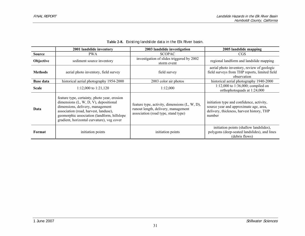
FINAL REPORT Landslide Hazards in the Elk River Basin Humboldt County, California
1 June 2007 Stillwater Sciences
31
Table 2-8. Existing landslide data in the Elk River basin.
2001 landslide inventory 2003 landslide investigation 2005 landslide mapping Source PWA SCOPAC CGS
Objective sediment source inventory investigation of slides triggered by 2002 storm event regional landform and landslide mapping
Methods aerial photo inventory, field survey field survey aerial photo inventory, review of geologic
field surveys from THP reports, limited field observation
Base data historical aerial photography 1954-2000 2003 color air photos historical aerial photography 1940-2000
Scale 1:12,000 to 1:21,120 1:12,000 1:12,000 to 1:36,000; compiled on orthophotoquads at 1:24,000
Data
feature type, certainty, photo year, erosion dimensions (L, W, D, V), depositional dimensions, delivery, management association (road, harvest, landuse), geomorphic association (landform, hillslope gradient, horizontal curvature), veg cover
feature type, activity, dimensions (L, W, D), runout length, delivery, management association (road type, stand type)
initiation type and confidence, activity, source year and approximate age, area, delivery, thickness, harvest history, THP number
Format initiation points initiation points initiation points (shallow landslides),
polygons (deep-seated landslides), and lines (debris flows)
FINAL REPORT Landslide Hazards in the Elk River Basin Humboldt County, California
1 June 2007 Stillwater Sciences
32
2.4.2 Deep-seated landslide modeling
DSLED-Rough and DSLED-Drain modeling approaches are in development and have not been extensively or systematically tested using independent deep-seated landslide data sources. Testing of model results for potential deep-seated hillslope instability were limited by available deep-seated landslide mapping in the Project Area. After comparison of modeling results with mapped deep-seated features mapped by CGS (Marshall and Mendes 2005) and discussion of alternative approaches, it was determined that there is currently insufficient information to objectively test the modeling results using existing landslide mapping. This is largely due to uncertainties in the types, boundaries, and activity level of existing deep-seated landslide mapping. Evaluation of deep-seated model performance in later sections of this report are therefore qualitative.
FINAL REPORT Landslide Hazards in the Elk River Basin Humboldt County, California
1 June 2007 Stillwater Sciences
33
3 RESULTS
3.1 Shallow Landslide Modeling Results
Four distributed, physically-based models were employed to predict potential shallow landslide hazards in the Elk River basin: the deterministic models SHALSTAB and SHALSTAB.V, and the probabilistic models PISA and PISA.V. Results are based on topographic data obtained from a 4-m DEM constructed from LiDAR data and the parameter values discussed above. The spatial distribution and magnitude of log (q/T) results for SHALSTAB and SHALSTAB.V are shown in Figure 3-1 Figure 3-2, respectively. High, moderately high, and moderate potential instability are represented by areas where log q/T is less than or equal to -3.1, -2.8, and -2.5, respectively. These preliminary classes are based on suggested log(q/T) thresholds reported for SHALSTAB applications in other areas (Dietrich et al 2001, Montgomery et al. 1998). The pattern of potential instability predicted by SHASTAB and SHALSTAB.V is similar, where areas with relatively high potential for shallow instability generally occur on steep convergent slopes. SHALSTAB V focuses instability in steep, convergent areas with thicker soil mantle and predicts greater stability in divergent areas and less steep convergent areas with thinner soil mantle. The spatial distribution and magnitude of probability of failure predicted by PISA and PISA.V are shown in Figure 3-3 and Figure 3-4, respectively. Probability of failure classes shown for PISA and PISA.V were classified in order to best illustrate the range of potential instability. PISA.V results in notably lower probabilities of failure. The magnitude and distribution of the modeling results are further discussed and compared in the following sections on model testing.
3.2 Shallow Landslide Model Testing
3.2.1 Model performance based on p-tests
Statistical p-tests were used within a hypothesis testing framework to address two basic questions:
1. Do shallow landslide models predict greater potential instability at known slide locations than at random positions in the landscape?
2. Are the models better predictors of instability than predictions based solely on hillslope gradient?
To address the first question, model values for potential instability at mapped landslide points were tested against model values of potential instability at a set of random points sampled within the Elk River Project Area. To address the second question, model values for potential instability at mapped landslide points were tested against model values for potential instability at a set of random points sampled from a probability distribution of potentially unstable slopes defined by hillslope gradient at landslide points (Appendix A). A p-test value of less than 0.5 (p<0.5) means
FINAL REPORT Landslide Hazards in the Elk River Basin Humboldt County, California
1 June 2007 Stillwater Sciences
34
that the model value at a landslide point predicted higher potential instability than model values at more than half of the 5,000 random points. P-test results for individual landslides are shown in Appendix B for tests conducted based on randomly sampled points, and in Appendix c for tests conducted based on points randomly sampled from a distribution of potentially unstable slopes. Reliable model validation based on p-testing was not possible in Franciscan Complex Central Belt due to the small sample size (n=6) for non-road-related shallow landslide initiation points in that terrain. Table 3-1 summarizes the percent of shallow landslides in each geologic terrain where p<0.5. The percent of shallow landslides where p <0.5 was significantly higher when p-tests were based on the highest potential instability (most limiting) within an 8-meter radius of a point rather than instability at a point, and we assume hereafter that maximum instability within a radius is more representation of model performance. A second percentage (reported in parentheses in Table 3-1) was calculated after removing landslides where p>0.5 for all four models, indicating poor performance for all models. In removing these landslide points, we assume they are not located accurately enough to encompass the landslide initiation area (limiting instability) within an 8-m radius and are therefore less useful in evaluating model performance. For three of the four models (SHALSTAB, SHALSTAB.V, and PISA), p-values based on random sampling were less than 0.5 for 73% or more of the landslide points. In other words, for 73% or more of the landslides in a given terrain, all three models predicted greater potential instability at the slide point than at more than half of the random points. This percentage increased to 82% or more when considering only landslides where p<0.5 for at least one model. When P-tests were conducted by randomly sampling points from a distribution of potentially unstable slopes (defined by hillslope gradient at landslide points), p values were still <0.5 for 64% or more landslide points, and 75% or more landslide points where p<0.5 for at least one model. These p-test results statistically demonstrate that (1) shallow landslide models do predict greater potential instability at known slide locations than at random locations, and (2) the models are significantly better predictors of potential instability than predictions based solely on hillslope gradient. The performance of shallow landslide models relative to each other was determined for each geologic terrain based on comparison of p-test values, where the relative performance is defined as the percent of shallow landslides with p<0.5.(Tables 3-2 , 3-3, and 3-4). The following results are apparent when comparing p-test results based on the highest (most limiting) instability within an 8-meter radius of a point and using only landslide points where p<0.5 for at least one model:
• Qh-Qmts-Qrt terrain: SHALSTAB.V and PISA.V both performed better than other models. Differences between SHALSTAB.V and PISA.V, however, were small (within 3%). Differences between PISA and PISA.V were also small (within 3%).
• Qtwu terrain: SHALSTAB.V and PISA both performed better than other models. Differences between SHALSTAB.V and PISA, however, were small (within 3%).
• Ty terrain: SHALSTAB.V performed significantly better than PISA. Differences in all other model comparisons were small (within 3%).
In summary, comparisons of model performance based on p-values indicate that SHALSTAB.V is the best-performing deterministic model and PISA is typically the best-performing probabilistic model. Differences between SHALSTAB.V and PISA are typically small (within 3%).
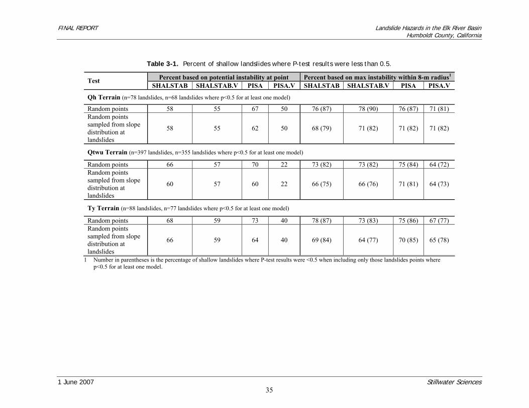
FINAL REPORT Landslide Hazards in the Elk River Basin Humboldt County, California
1 June 2007 Stillwater Sciences
35
Table 3-1. Percent of shallow landslides where P-test results were less than 0.5.
Percent based on potential instability at point Percent based on max instability within 8-m radius1 Test SHALSTAB SHALSTAB.V PISA PISA.V SHALSTAB SHALSTAB.V PISA PISA.V
Qh Terrain (n=78 landslides, n=68 landslides where p<0.5 for at least one model)
Random points 58 55 67 50 76 (87) 78 (90) 76 (87) 71 (81) Random points sampled from slope distribution at landslides
58 55 62 50 68 (79) 71 (82) 71 (82) 71 (82)
Qtwu Terrain (n=397 landslides, n=355 landslides where p<0.5 for at least one model)
Random points 66 57 70 22 73 (82) 73 (82) 75 (84) 64 (72) Random points sampled from slope distribution at landslides
60 57 60 22 66 (75) 66 (76) 71 (81) 64 (73)
Ty Terrain (n=88 landslides, n=77 landslides where p<0.5 for at least one model)
Random points 68 59 73 40 78 (87) 73 (83) 75 (86) 67 (77) Random points sampled from slope distribution at landslides
66 59 64 40 69 (84) 64 (77) 70 (85) 65 (78)
1 Number in parentheses is the percentage of shallow landslides where P-test results were <0.5 when including only those landslides points where p<0.5 for at least one model.
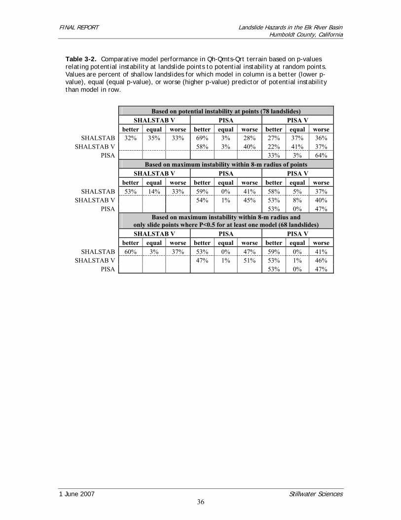
FINAL REPORT Landslide Hazards in the Elk River Basin Humboldt County, California
1 June 2007 Stillwater Sciences
36
Table 3-2. Comparative model performance in Qh-Qmts-Qrt terrain based on p-values relating potential instability at landslide points to potential instability at random points. Values are percent of shallow landslides for which model in column is a better (lower p-value), equal (equal p-value), or worse (higher p-value) predictor of potential instability than model in row.
Based on potential instability at points (78 landslides)
SHALSTAB V PISA PISA V better equal worse better equal worse better equal worse
SHALSTAB 32% 35% 33% 69% 3% 28% 27% 37% 36% SHALSTAB V 58% 3% 40% 22% 41% 37%
PISA 33% 3% 64% Based on maximum instability within 8-m radius of points
SHALSTAB V PISA PISA V better equal worse better equal worse better equal worse
SHALSTAB 53% 14% 33% 59% 0% 41% 58% 5% 37% SHALSTAB V 54% 1% 45% 53% 8% 40%
PISA 53% 0% 47% Based on maximum instability within 8-m radius and
only slide points where P<0.5 for at least one model (68 landslides) SHALSTAB V PISA PISA V
better equal worse better equal worse better equal worse SHALSTAB 60% 3% 37% 53% 0% 47% 59% 0% 41%
SHALSTAB V 47% 1% 51% 53% 1% 46% PISA 53% 0% 47%
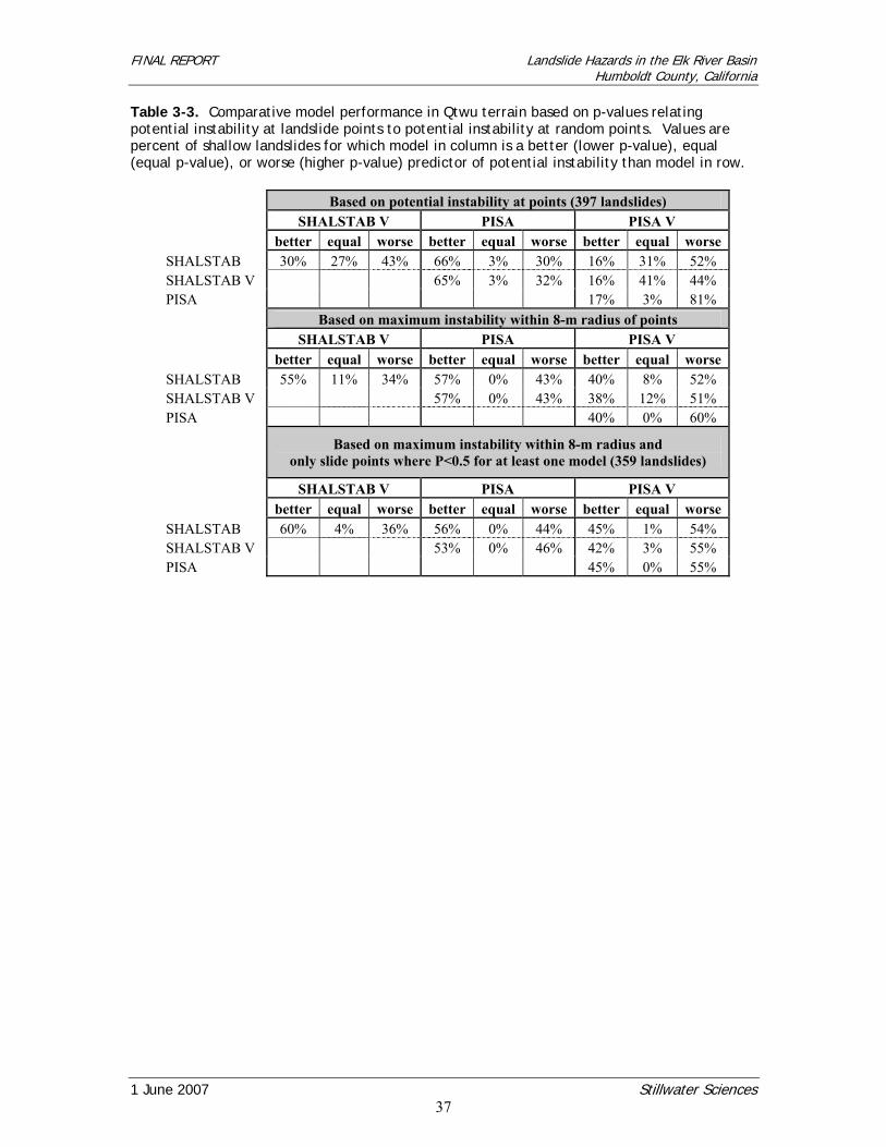
FINAL REPORT Landslide Hazards in the Elk River Basin Humboldt County, California
1 June 2007 Stillwater Sciences
37
Table 3-3. Comparative model performance in Qtwu terrain based on p-values relating potential instability at landslide points to potential instability at random points. Values are percent of shallow landslides for which model in column is a better (lower p-value), equal (equal p-value), or worse (higher p-value) predictor of potential instability than model in row.
Based on potential instability at points (397 landslides)
SHALSTAB V PISA PISA V better equal worse better equal worse better equal worseSHALSTAB 30% 27% 43% 66% 3% 30% 16% 31% 52% SHALSTAB V 65% 3% 32% 16% 41% 44% PISA 17% 3% 81%
Based on maximum instability within 8-m radius of points SHALSTAB V PISA PISA V
better equal worse better equal worse better equal worseSHALSTAB 55% 11% 34% 57% 0% 43% 40% 8% 52% SHALSTAB V 57% 0% 43% 38% 12% 51% PISA 40% 0% 60%
Based on maximum instability within 8-m radius and only slide points where P<0.5 for at least one model (359 landslides)
SHALSTAB V PISA PISA V better equal worse better equal worse better equal worseSHALSTAB 60% 4% 36% 56% 0% 44% 45% 1% 54% SHALSTAB V 53% 0% 46% 42% 3% 55% PISA 45% 0% 55%
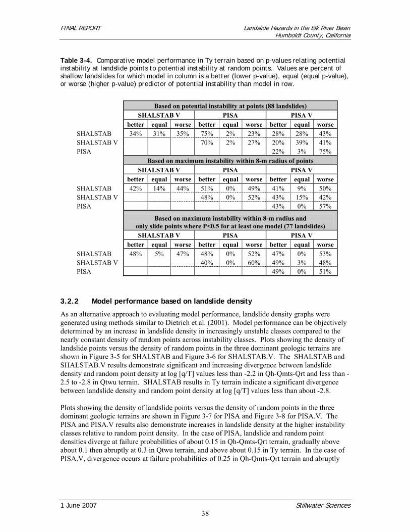
FINAL REPORT Landslide Hazards in the Elk River Basin Humboldt County, California
1 June 2007 Stillwater Sciences
38
Table 3-4. Comparative model performance in Ty terrain based on p-values relating potential instability at landslide points to potential instability at random points. Values are percent of shallow landslides for which model in column is a better (lower p-value), equal (equal p-value), or worse (higher p-value) predictor of potential instability than model in row.
Based on potential instability at points (88 landslides)
SHALSTAB V PISA PISA V better equal worse better equal worse better equal worseSHALSTAB 34% 31% 35% 75% 2% 23% 28% 28% 43% SHALSTAB V 70% 2% 27% 20% 39% 41% PISA 22% 3% 75%
Based on maximum instability within 8-m radius of points SHALSTAB V PISA PISA V
better equal worse better equal worse better equal worseSHALSTAB 42% 14% 44% 51% 0% 49% 41% 9% 50% SHALSTAB V 48% 0% 52% 43% 15% 42% PISA 43% 0% 57%
Based on maximum instability within 8-m radius and only slide points where P<0.5 for at least one model (77 landslides) SHALSTAB V PISA PISA V
better equal worse better equal worse better equal worseSHALSTAB 48% 5% 47% 48% 0% 52% 47% 0% 53% SHALSTAB V 40% 0% 60% 49% 3% 48% PISA 49% 0% 51%
3.2.2 Model performance based on landslide density
As an alternative approach to evaluating model performance, landslide density graphs were generated using methods similar to Dietrich et al. (2001). Model performance can be objectively determined by an increase in landslide density in increasingly unstable classes compared to the nearly constant density of random points across instability classes. Plots showing the density of landslide points versus the density of random points in the three dominant geologic terrains are shown in Figure 3-5 for SHALSTAB and Figure 3-6 for SHALSTAB.V. The SHALSTAB and SHALSTAB.V results demonstrate significant and increasing divergence between landslide density and random point density at log [q/T] values less than -2.2 in Qh-Qmts-Qrt and less than -2.5 to -2.8 in Qtwu terrain. SHALSTAB results in Ty terrain indicate a significant divergence between landslide density and random point density at log [q/T] values less than about -2.8. Plots showing the density of landslide points versus the density of random points in the three dominant geologic terrains are shown in Figure 3-7 for PISA and Figure 3-8 for PISA.V. The PISA and PISA.V results also demonstrate increases in landslide density at the higher instability classes relative to random point density. In the case of PISA, landslide and random point densities diverge at failure probabilities of about 0.15 in Qh-Qmts-Qrt terrain, gradually above about 0.1 then abruptly at 0.3 in Qtwu terrain, and above about 0.15 in Ty terrain. In the case of PISA.V, divergence occurs at failure probabilities of 0.25 in Qh-Qmts-Qrt terrain and abruptly

FINAL REPORT Landslide Hazards in the Elk River Basin Humboldt County, California
1 June 2007 Stillwater Sciences
39
from the origin in Qtwu terrain. Landslide densities area not reported for Ty terrain due to the small number of landslides mapped in different probability classes within that terrain
3.2.3 Correct landslide prediction versus area predicted to be unstable
The fraction of watershed area encompassed by a model-predicted potential instability value (log (q/T) or probability of failure) relative to the number of mapped landslides correctly predicted by that instability value is a useful measure for determining relevant landslide hazard classes (Dietrich et al. 2001). The approach considers both (1) the extent to which a model threshold correctly classifies mapped landslides as unstable and (2) the potential over prediction of unstable area. Figure 3-9 and Figure 3-10 show the cumulative percent area and cumulative percent of mapped landslides in the Elk River watershed for potential instability predicted by SHALSTAB, SHALSTAB V, PISA, and PISA V (Table 3-5). Figure 3-11 shows cumulative percent of watershed area plotted as a function of the cumulative percent of landslides correctly predicted by a given potential instability value. SHALSTAB and SHALSTAB V values are plotted for classes used in validation tests in the Coast Ranges of California and Oregon (Dietrich et al. 2001). PISA and PISA V classes are plotted at intervals within the range of probability of sliding values encompassing the majority of landslides in the Elk River basin (0–0.5). SHALSTAB V results in the Elk River basin, when compared to previous SHALSTAB validation studies in similar terrain, correctly predict fewer landslides and classify less of the watershed area as unstable for a given log (q/T) threshold. Dietrich et al. (2001) found that for 7 watersheds in the northern California Coast Range, the cumulative percentage of mapped in-unit landslides for the less than -3.1, -2.8, and –2.5 categories was 46, 58, and 73 percent, respectively. The cumulative area covered by the less than -3.1, -2.8, and –2.5 categories was 11.4, 16, and 25.7 percent, respectively. A study of 629 landslides in Washington Coast Range found that 86% of the slides occurred within log (q/T) less than -2.5 using 30-m data (K. Sullivan, pers. com., 1994 as cited in Dietrich et al. 2001). Montgomery et al. (1998), found that when SHALSTAB was tested against 3,224 landslides in 14 watersheds of the Oregon and Washington Coast Ranges, about 66% of the landslides occurred within log (q/T) less than -2.5 using 30-m grid data. In comparison, the cumulative percentage of landslides in the less than -3.1, -2.8, and –2.5 categories in the Elk River basin was 10, 19, and 29 percent, respectively; and the area covered by the less than -3.1, -2.8, and –2.5 categories was 3, 6, and 13 percent, respectively (Table 3-5). Discrepancies between validation results reported for the Elk River basin and those reported for other areas are likely due to (1) uncertainties in the actual location of shallow landslide initiation relative to the mapped landslide points used to test model results; (2) differences in the resolution of topography used in mapping, modeling, and model testing; and (3) differences between the processes controlling model-predicted potential instability (shallow failure in areas with steep, convergent topography and thick soil accumulation) and the processes controlling shallow landsliding in the Elk River basin.
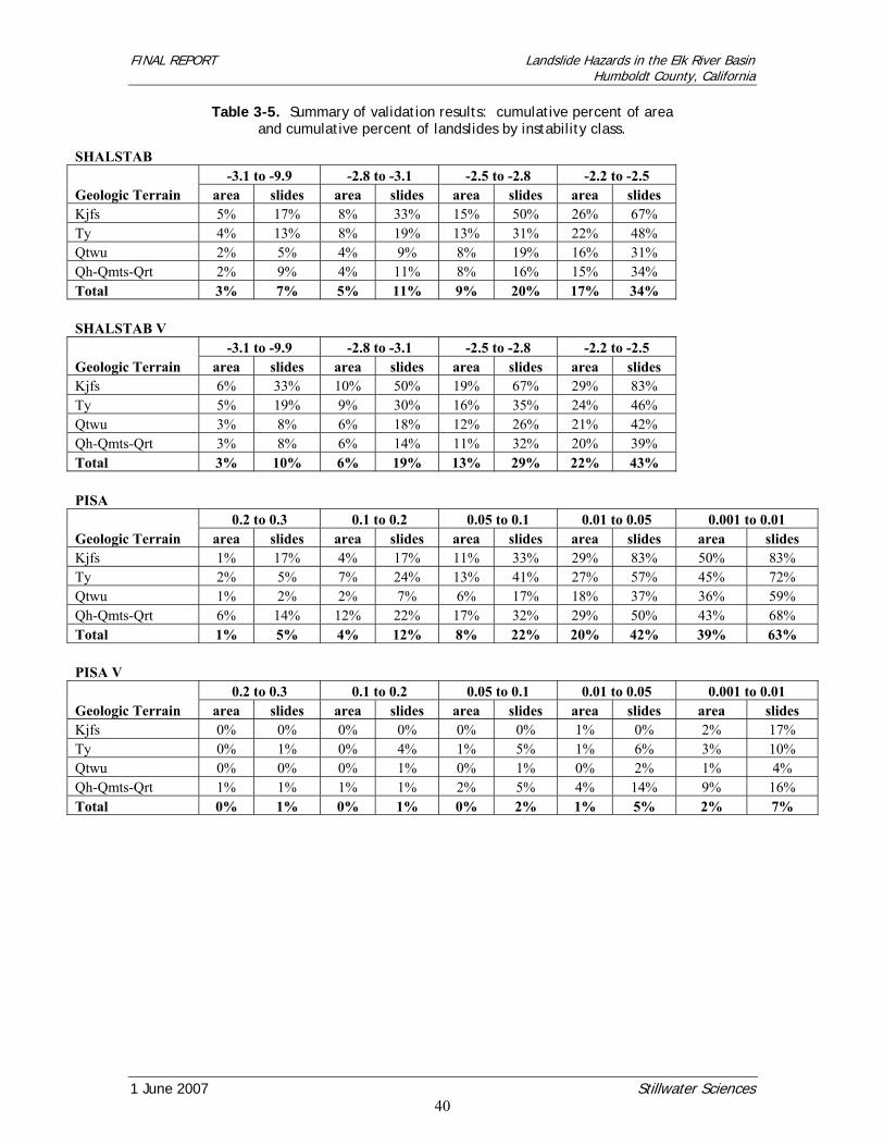
FINAL REPORT Landslide Hazards in the Elk River Basin Humboldt County, California
1 June 2007 Stillwater Sciences
40
Table 3-5. Summary of validation results: cumulative percent of area and cumulative percent of landslides by instability class.
SHALSTAB -3.1 to -9.9 -2.8 to -3.1 -2.5 to -2.8 -2.2 to -2.5 Geologic Terrain area slides area slides area slides area slides Kjfs 5% 17% 8% 33% 15% 50% 26% 67% Ty 4% 13% 8% 19% 13% 31% 22% 48% Qtwu 2% 5% 4% 9% 8% 19% 16% 31% Qh-Qmts-Qrt 2% 9% 4% 11% 8% 16% 15% 34% Total 3% 7% 5% 11% 9% 20% 17% 34% SHALSTAB V -3.1 to -9.9 -2.8 to -3.1 -2.5 to -2.8 -2.2 to -2.5 Geologic Terrain area slides area slides area slides area slides Kjfs 6% 33% 10% 50% 19% 67% 29% 83% Ty 5% 19% 9% 30% 16% 35% 24% 46% Qtwu 3% 8% 6% 18% 12% 26% 21% 42% Qh-Qmts-Qrt 3% 8% 6% 14% 11% 32% 20% 39% Total 3% 10% 6% 19% 13% 29% 22% 43% PISA 0.2 to 0.3 0.1 to 0.2 0.05 to 0.1 0.01 to 0.05 0.001 to 0.01 Geologic Terrain area slides area slides area slides area slides area slides Kjfs 1% 17% 4% 17% 11% 33% 29% 83% 50% 83% Ty 2% 5% 7% 24% 13% 41% 27% 57% 45% 72% Qtwu 1% 2% 2% 7% 6% 17% 18% 37% 36% 59% Qh-Qmts-Qrt 6% 14% 12% 22% 17% 32% 29% 50% 43% 68% Total 1% 5% 4% 12% 8% 22% 20% 42% 39% 63% PISA V 0.2 to 0.3 0.1 to 0.2 0.05 to 0.1 0.01 to 0.05 0.001 to 0.01 Geologic Terrain area slides area slides area slides area slides area slides Kjfs 0% 0% 0% 0% 0% 0% 1% 0% 2% 17% Ty 0% 1% 0% 4% 1% 5% 1% 6% 3% 10% Qtwu 0% 0% 0% 1% 0% 1% 0% 2% 1% 4% Qh-Qmts-Qrt 1% 1% 1% 1% 2% 5% 4% 14% 9% 16% Total 0% 1% 0% 1% 0% 2% 1% 5% 2% 7%
FINAL REPORT Landslide Hazards in the Elk River Basin Humboldt County, California
1 June 2007 Stillwater Sciences
41
The sampling approach outlined in Section 2.4.1.3 was independently used to determine a threshold for managing landslide hazard that minimizes the total cost associated with incorrect slide classification and over prediction of potentially unstable area. Table 3-6 summarizes confidence intervals for threshold values and the associated cumulative fraction of slides or random points classified by the threshold value (refer also to Appendix E). The 95% confidence intervals are based on the 2.5 percentile and 97.5 percentile from 5000 bootstrap iterations. Log(q/T) thresholds for SHALSTAB and SHALSTAB.V based on the sampling approach are similar for a given geologic terrain, ranging from -2.1 in Qh-Qmts-Qrt terrain to -2.5 in Ty terrain (Table 3-5). RS(x) and RL(x) for the inferred SHALSTAB and SHALSTAB.V thresholds were also similar for a given geologic terrain (Table 3-6). Threshold values determined by the RS(x)-RL(x) method, however, were lower, and therefore more conservative than suggested log(q/T) thresholds reported for SHALSTAB applications in other areas (Dietrich et al 2001, Shaw and Vaugeois 1999, Montgomery et al. 1998). Dietrich et al. (2001), for example, recommend using a log (q/T) threshold of -2.5 or lower (more unstable). Probability of failure thresholds for PISA and PISA.V based on the sampling approach varied for a given geologic terrain (Table 3-6). PISA thresholds ranged from 0.06 in Qtwu terrain to 0.10 in Ty terrain and 0.17 in Qh-Qmts-Qrt terrain. PISA.V thresholds were lower, ranging from 0.02 in Qtwu terrain to 0.14 in Qh-Qmts-Qrt terrain. RS(x) and RL(x) for the inferred PISA.V thresholds were lower than for inferred PISA thresholds (Table 3-6). Threshold values for PISA determined by the sampling approach were lower than probability of failure thresholds reported for PISA applications in other areas. Haneberg (2004) found that in the Wheeling area of West Virginia, the correspondence between active landslide area and probabilities of sliding at the 0.5, 0.3, and 0.1 thresholds was approximately 64, 89, and 99 percent respectively. These results, however, report the distribution of calculated probability of sliding values for each hazard unit, and may not be directly comparable to RS(x) and RL(x) reported here for the Elk River basin.
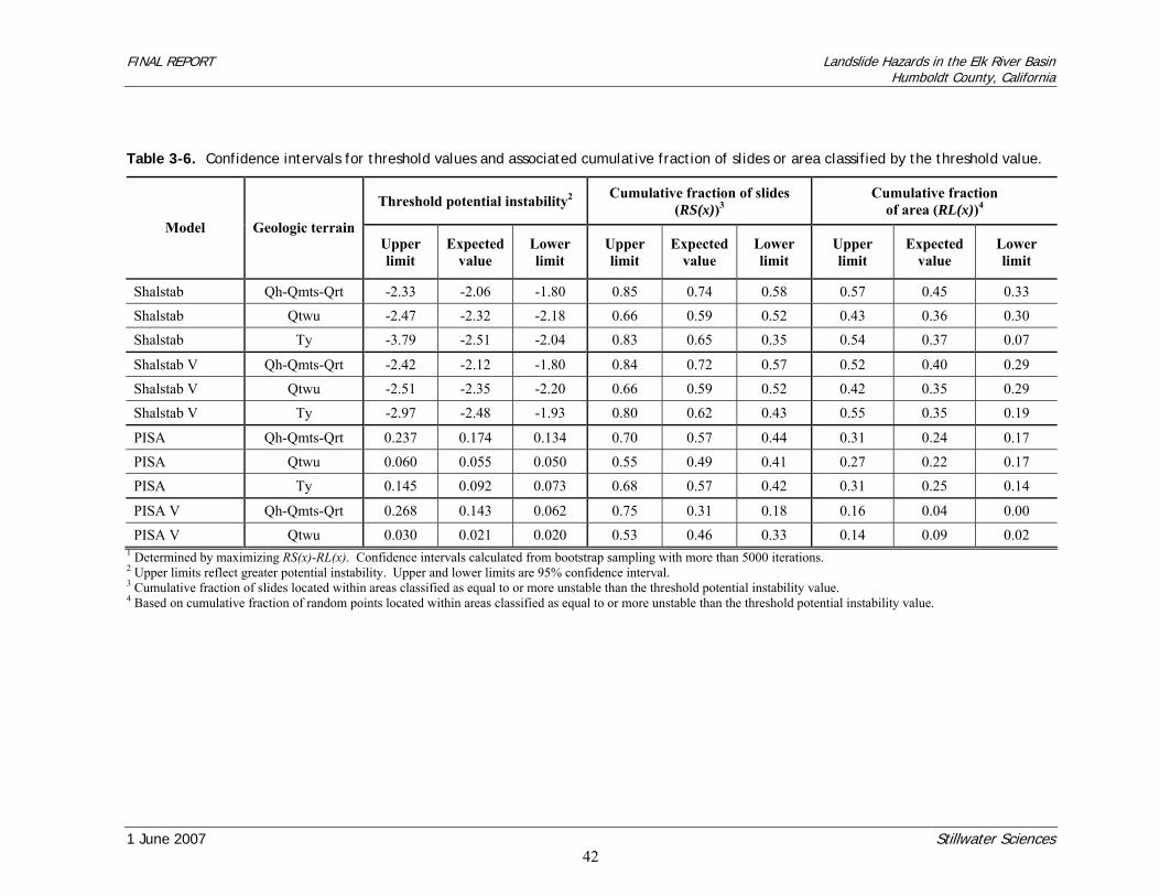
FINAL REPORT Landslide Hazards in the Elk River Basin Humboldt County, California
1 June 2007 Stillwater Sciences
42
Table 3-6. Confidence intervals for threshold values and associated cumulative fraction of slides or area classified by the threshold value.
Threshold potential instability2 Cumulative fraction of slides (RS(x))3
Cumulative fraction of area (RL(x))4
Model Geologic terrain Upper limit
Expected value
Lower limit
Upper limit
Expected value
Lower limit
Upper limit
Expected value
Lower limit
Shalstab Qh-Qmts-Qrt -2.33 -2.06 -1.80 0.85 0.74 0.58 0.57 0.45 0.33
Shalstab Qtwu -2.47 -2.32 -2.18 0.66 0.59 0.52 0.43 0.36 0.30
Shalstab Ty -3.79 -2.51 -2.04 0.83 0.65 0.35 0.54 0.37 0.07
Shalstab V Qh-Qmts-Qrt -2.42 -2.12 -1.80 0.84 0.72 0.57 0.52 0.40 0.29
Shalstab V Qtwu -2.51 -2.35 -2.20 0.66 0.59 0.52 0.42 0.35 0.29
Shalstab V Ty -2.97 -2.48 -1.93 0.80 0.62 0.43 0.55 0.35 0.19
PISA Qh-Qmts-Qrt 0.237 0.174 0.134 0.70 0.57 0.44 0.31 0.24 0.17
PISA Qtwu 0.060 0.055 0.050 0.55 0.49 0.41 0.27 0.22 0.17
PISA Ty 0.145 0.092 0.073 0.68 0.57 0.42 0.31 0.25 0.14
PISA V Qh-Qmts-Qrt 0.268 0.143 0.062 0.75 0.31 0.18 0.16 0.04 0.00
PISA V Qtwu 0.030 0.021 0.020 0.53 0.46 0.33 0.14 0.09 0.02 1 Determined by maximizing RS(x)-RL(x). Confidence intervals calculated from bootstrap sampling with more than 5000 iterations. 2 Upper limits reflect greater potential instability. Upper and lower limits are 95% confidence interval. 3 Cumulative fraction of slides located within areas classified as equal to or more unstable than the threshold potential instability value. 4 Based on cumulative fraction of random points located within areas classified as equal to or more unstable than the threshold potential instability value.
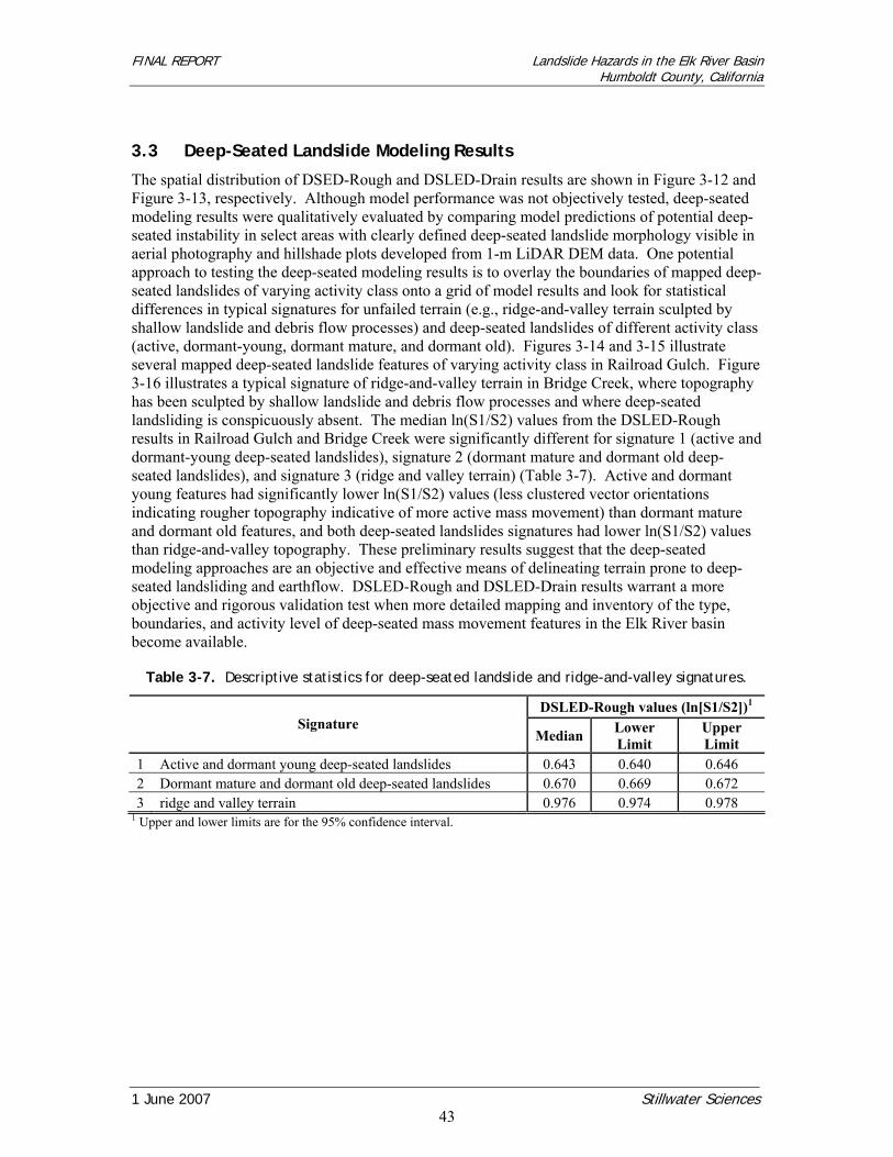
FINAL REPORT Landslide Hazards in the Elk River Basin Humboldt County, California
1 June 2007 Stillwater Sciences
43
3.3 Deep-Seated Landslide Modeling Results
The spatial distribution of DSED-Rough and DSLED-Drain results are shown in Figure 3-12 and Figure 3-13, respectively. Although model performance was not objectively tested, deep-seated modeling results were qualitatively evaluated by comparing model predictions of potential deep-seated instability in select areas with clearly defined deep-seated landslide morphology visible in aerial photography and hillshade plots developed from 1-m LiDAR DEM data. One potential approach to testing the deep-seated modeling results is to overlay the boundaries of mapped deep-seated landslides of varying activity class onto a grid of model results and look for statistical differences in typical signatures for unfailed terrain (e.g., ridge-and-valley terrain sculpted by shallow landslide and debris flow processes) and deep-seated landslides of different activity class (active, dormant-young, dormant mature, and dormant old). Figures 3-14 and 3-15 illustrate several mapped deep-seated landslide features of varying activity class in Railroad Gulch. Figure 3-16 illustrates a typical signature of ridge-and-valley terrain in Bridge Creek, where topography has been sculpted by shallow landslide and debris flow processes and where deep-seated landsliding is conspicuously absent. The median ln(S1/S2) values from the DSLED-Rough results in Railroad Gulch and Bridge Creek were significantly different for signature 1 (active and dormant-young deep-seated landslides), signature 2 (dormant mature and dormant old deep-seated landslides), and signature 3 (ridge and valley terrain) (Table 3-7). Active and dormant young features had significantly lower ln(S1/S2) values (less clustered vector orientations indicating rougher topography indicative of more active mass movement) than dormant mature and dormant old features, and both deep-seated landslides signatures had lower ln(S1/S2) values than ridge-and-valley topography. These preliminary results suggest that the deep-seated modeling approaches are an objective and effective means of delineating terrain prone to deep-seated landsliding and earthflow. DSLED-Rough and DSLED-Drain results warrant a more objective and rigorous validation test when more detailed mapping and inventory of the type, boundaries, and activity level of deep-seated mass movement features in the Elk River basin become available.
Table 3-7. Descriptive statistics for deep-seated landslide and ridge-and-valley signatures.
DSLED-Rough values (ln[S1/S2])1 Signature
Median Lower Limit
Upper Limit
1 Active and dormant young deep-seated landslides 0.643 0.640 0.646 2 Dormant mature and dormant old deep-seated landslides 0.670 0.669 0.672 3 ridge and valley terrain 0.976 0.974 0.978
1 Upper and lower limits are for the 95% confidence interval.
FINAL REPORT Landslide Hazards in the Elk River Basin Humboldt County, California
1 June 2007 Stillwater Sciences
44
4 LANDSLIDE HAZARDS IN THE ELK RIVER BASIN
This report summarizes spatially distributed modeling of potential instability conducted in the Elk River Basin to assist in assigning a set of landslide hazard classes that will be used in developing a sediment TMDL and related strategy for recovery of sediment impaired beneficial uses in the Elk River basin. Mechanistic/physically-based modeling was conducted using the best available topographic data (4-m grid from LiDAR data), and model results were tested using the best available landslide data. Modeling and model testing results from this report will be integrated by NRWQCB to define landslide hazards that can be combined with information about sediment delivery and vulnerability of receptors to sediment impairment in assessing risk as part of TMDL analysis and implementation in Elk River. Landslide hazard, in this context, refers to the potential for occurrence of a damaging landslide within a given area; such damage could include loss of life or injury, property damage, social and economic disruption, or environmental degradation (National Research Council 2004). Landslide hazard classes will be integrated by normalizing results from the best-performing deterministic (SHALSTAB and SHALSTAB.V) and probabilistic (PISA and PISA.V) model approaches. P-tests and comparisons of landslide density to random point density in each instability class statistically demonstrate that (1) shallow landslide models predict greater instability at landslide initiation sites than at randomly selected points, and (2) the models are significantly better predictors of potential shallow instability than predictions based solely on hillslope gradient. P-tests indicated that three of the four models (SHALSTAB, SHALSTAB.V, and PISA) predicted greater instability at 82% or more of the landslide initiation sites than at randomly selected points (Table 3-1).1 When p-tests were conducted by randomly sampling points from a distribution of potentially unstable slopes (defined by hillslope gradient at landslide points), these models predicted greater instability at 75% or more of the landslide initiation sites (Table 3-1).1 Landslide densities significantly increased above random point densities at the log [q/T] values of about -2.5 to -2.8 using SHALSTAB and SHALSTAB.V (Figures 3-5 and 3-6), and at failure probabilities of about 0.15 to 0.3 using PISA (Figures 3-7and 3-8). Comparisons of model performance based on p-tests indicated that SHALSTAB.V was the best performing deterministic model and PISA was the best performing probabilistic model (Tables 3-2 through 3-4). Previous SHALSTAB validation studies have suggested potential log q/T thresholds from -2.2 to -3.1. In terms of correct landslide prediction and cumulative area encompassed by potential instability in the Elk River watershed, PISA probabilities of 0.01 to 0.10 are comparable to SHALSTAB V log (q/T) –2.2 to –3.1 (Table 3-5, Figure 3-11). SHALSTAB V results in the Elk River basin, however, correctly classified fewer landslides and less of the watershed area as unstable for a given log (q/T) threshold compared to previous SHALSTAB validation studies in similar terrain. Bootstrap samples of model predicted instability in the vicinity of slides and randomly selected points were used to assess thresholds for managing landslide hazard that minimize the total costs associated with incorrect slide classification and over prediction of potentially unstable area.
1 Results summarized here are based on p<0.5, maximum instability within 8-m radius, and include only landslides where p<0.5 for at least one model. Refer to Section 2.4.1 for a description of p-test methods and Section 3.2.1 for p-test results.
FINAL REPORT Landslide Hazards in the Elk River Basin Humboldt County, California
1 June 2007 Stillwater Sciences
45
Log(q/T) thresholds for SHALSTAB.V based on the bootstrap sampling approach ranged from -2.12 in Qh-Qmts-Qrt terrain to -2.48 in Ty terrain to -2.51 in Qtwu terrain (Table 3-5). PISA thresholds ranged from 0.06 in Qtwu terrain to 0.10 in Ty terrain to 0.17 in Qh-Qmts-Qrt terrain. Threshold values determined by the bootstrap sampling method were lower than suggested thresholds reported for SHALSTAB applications in other areas (Dietrich et al 2001, Montgomery et al. 1998).
4.1 Uses and Limitations
Although modeling of potential hillslope instability and assessment of potential landslide hazard thresholds is intended to inform resource agencies, land managers, and the public about hillslopes that are most sensitivity to management activities; the landslide hazard assessment does not assess how slopes will specifically respond to management-related slope alterations (drainage and excavation) or large seismic triggering events, both of which can increase hazard. Landslide hazard mapping is intended to show where further field investigation is necessary and prudent. Specific sites with higher and lower hazard may exist within any of the hazard classes, and hazard mapping should be used in combination with field geomorphic mapping and geotechnical investigations at specific locations. Hazard mapping is most applicable at the scale and resolution of the input data. This scale allows project level planning and review, but site-specific determination of landslide hazard and risk should be based on site-specific data and evaluation by qualified professionals. Lastly, landslide hazard mapping does not directly address potential sediment delivery from landslide-prone areas to a watercourse and/or other important receptors. Landslide hazard mapping, however, may be used in combination with information about hillslope and channel gradient and empirical data on sediment delivery to assess sediment delivery potential.
4.2 Future Analyses
Analysis of potential instability and delineation of landslide hazard is dependent on the precision, accuracy, and resolution of available information. Analyses in this report were conducted with best available information. However, many input parameters are poorly constrained and landslide data available for model testing are limited by spatial precision and accuracy. Analyses of landslide hazard can be improved in the future as the accuracy, precision, and resolution of input information improve over time. Specific areas for future improvement and research include the following:
• Root strength and the rate of root strength decay following disturbance is a large source of uncertainty in predictions of potential hillslope instability. More research is needed to better constrain root strength parameters for different vegetation cover types and root strength decay with time since disturbance (e.g., fire or timber harvest)
• This landslide hazard assessment evaluated potential instability of open slopes controlled primarily by topography and pore water pressure. More work is needed to assess how management-related slope alterations (road excavation and drainage) influence potential hillslope instability within different landslide hazard classes and geologic terrains.
• Correlation of the factors influencing hillslope instability to landslide occurrence on a watershed scale has historically been limited by the resolution of the topographic data available for mapping observed landslide initiation areas. High-resolution topographic data from LiDAR is now available to more accurately and precisely map the location of landslide initiation, erosional, and depositional areas in the Elk River basin. Landslide

FINAL REPORT Landslide Hazards in the Elk River Basin Humboldt County, California
1 June 2007 Stillwater Sciences
46
field and aerial photo inventories consisting of erosional and depositional map polygons registered to the same LiDAR topographic data used here to model potential instability would provide a better means of testing the modeling results and determining thresholds of instability for landslide hazard classes.
• More work is needed to develop methods of estimating sediment production and delivery under different management scenarios using the landslide hazard assessment in combination with other data sources.
• More work is needed to characterize the type, boundaries, timing, and activity level of deep-seated landslides in the basin in order to better validate the deep-seated model results and develop appropriate hazard classes.
FINAL REPORT Landslide Hazards in the Elk River Basin Humboldt County, California
1 June 2007 Stillwater Sciences
47
5 LITERATURE CITED
Bachman, S. B., M. B. Underwood, and J. S. Menack. 1984. Cenozoic evolution of coastal northern California. Pages 55-66 in J. K. Crouch and S. B. Bachman, editors. Tectonics and sedimentation along the California margin. Pacific Section Book Series, Volume 38. Society of Economic Paleontologists and Mineralogists, Los Angeles, California. Bedrossian, T. L. 1983. Watersheds mapping in northern California. California Geology 36: 140-147. Blake, M. C., Jr., A. S. Jayko, and R. J. McLaughlin. 1985. Tectonostratigraphic terranes of the northern coast ranges, California. Pages 159-171 in D. G. Howell, editor. Tectonostratigraphic terranes of the circum-Pacific region. Earth Sciences Series 1. Circum-Pacific Council for Energy and Mineral Resources. Bowman, A. W., and A. Azzalini. 1997. Applied smoothing techniques for data analysis: the kernel approach with S-Plus illustrations. Oxford Statistical Science Series No. 18. Clarendon Press, Oxford, England. Bowman, A. W., and A. Azzalini. 2005. Smoothing methods for nonparametric regression and density estimation. R package Version 2.1-0. Ported to R by B. D. Ripley up to Version 2.0. California Department of Conservation. 1999. Factors affecting landslides in forested terrain, Note 50. California Department of Conservation, Division of Mines and Geology, Sacramento, California. California Department of Forestry and Fire Protection. 2005. California Forest Practice Rules. Title 14, California Code of Regulations: Chapters 4, 4.5, and 10. Prepared by California Department of Forestry and Fire Protection Resource Management, Forest Practice Program, Sacramento, California, for California Licensed Timber Operators and California Registered Professional Foresters. Clarke, S. H., Jr., and G. A. Carver. 1992. Late Holocene tectonics and paleoseismicity, southern Cascadia subduction zone. Science 255: 188-192. Cruden, D. M., and D. J. Varnes. 1996. Landslide types and processes. Pages 36-75 in Landslides investigation and mitigation. Special Report 247. Transportation Research Board, Washington, D. C. De la Fuente, J., D. Elder, and A. Miller. 2002. Does deforestation influence the activity of deep-seated landslides? Observations from the flood of 1997 in the central Klamath Mountains, northern California. Abstracts with Programs - Geological Society of America 34: 88. Dhakal, A. S., and R. C. Sidle. 2003. Long-term modeling of landslides for different forest management practices. Earth Surface Processes and Landforms 28: 853-868.
FINAL REPORT Landslide Hazards in the Elk River Basin Humboldt County, California
1 June 2007 Stillwater Sciences
48
Dietrich, W. E., D. Bellugi, and R. Real de Asua. 2001. Validation of the shallow landslide model, SHALSTAB, for forest management. Pages 195-227 in Land use and watersheds: human influence on hydrology and geomorphology in urban and forest areas. American Geophysical Union. Dietrich, W. E., and D. R. Montgomery. 1998. SHALSTAB: a digital terrain model for mapping shallow landslide potential. Prepared for publication as a technical report by NCASI. Dietrich, W. E., R. Reiss, M.-L. Hsu, and D. R. Montgomery. 1995. A process-based model for colluvial soil depth and shallow landsliding using digital elevation data. Hydrological Processes 9: 383-400. Earth Science Associates. 1975. Geology of the Humboldt Bay region. Prepared for Pacific Gas & Electric Company Hammond, C., D. Hall, S. Miller, and P. Swetik. 1992. Level I stability analysis (LISA) documentation for Version 2.0. General Technical Report INT-285. USDA Forest Service, Intermountain Research Station, Ogden, Utah. Haneberg, W. C. 2000. Deterministic and probabilistic approaches to geologic hazard assessment. Environmental and Engineering Geoscience VI: 209-226. Haneberg, W. C. 2004. A rational probabilistic method for spatially distributed landslide hazard assessment. Environmental and Engineering Geoscience X: 27-43. Haneberg, W. C. 2005. PISA: probabilistic infinite slope analysis, user manual. Version 1.0. Haneberg Geoscience. Heimsath, A. M., W. E. Dietrich, K. Nishiizumi, and R. C. Finkel. 1997. The soil production function and landscape equilibrium. Nature 388: 358-361. Heimsath, A. M., W. E. Dietrich, K. Nishiizumi, and R. C. Finkel. 2001. Stochastic processes of soil production and transport: erosion rates, topographic variation and cosmogenic nuclides in the Oregon Coast Range. Earth Surface Processes and Landforms 26: 531-552. Heimsath, A. M., W. E. Dietrich, and L. Nishiizumi. 1999. Cosmogenic nuclides, topography, and the spatial variation of soil depth. Geomorphology 27: 151-172. Ingle, J. C., Jr. 1987. The depositional, tectonic, and paleoceanography history of the Eel River (Humboldt), Point Arena, and Bodega (Point Reyes) basins of northern California; a summary of stratigraphic evidence. H. Schymiczek and R. Suchsland, editors. Tectonics, sedimentation and evolution of the Eel River and associated coastal basins of northern California. San Joaquin Geological Society, Bakersfield, California. Jayco, A. S., and Jr. M. C. Blake. 1987. Geologic terranes of coastal northern California and southern Oregon. H. Schymiczek and R. Suchsland, editors. Tectonics, sedimentation and evolution of the Eel River and associated coastal basins of northern California. San Joaquin Geological Society, Bakersfield, California.
FINAL REPORT Landslide Hazards in the Elk River Basin Humboldt County, California
1 June 2007 Stillwater Sciences
49
Klein, R. D., and J. K. Anderson. 1999. Channel migration zone delineation pilot study on North Fork Eel River. Review draft. Prepared for Scotia Pacific Company, LLC. Mackey, B. H., J. J. Roering, and W. E. Dietrich. 2005. Determining the topographic manifestation of widespread landsliding with high resolution airborne laser swath mapping (ALSM) data, South Fork Eel River, northern California. American Geophysical Union Fall Meeting 2005: abstract #H34B-04. Mackey, B. H., J. J. Roering, J. McKean, and W. E. Dietrich. 2006. Analyzing the spatial pattern of deep-seated landsliding - evidence for base level control, South Fork Eel River, California. American Geophysical Union Fall Meeting 2006: abstract #H53B-0619. Marshall, G. J., and E. Mendes. 2005. Geologic and geomorphic features related to landsliding and landslide potential in the Eel River watershed. State of California, Department of Conservation, California Geological Survey, Sacramento, California. McCrory, P. A. 1989. Late Neogene geohistory analysis of the Humboldt basin and its relationships to convergence of the Jaun de Fuca plate. Journal of Geophysical Research 94: 3126-3138. McKean, J., and J. Roering. 2004. Objective landslide detection and surface morphology mapping using high-resolution airborne laser altimetry. Geomorphology 57: 331-351. McLaughlin, J. W., M. R. Gale, and C. C. Trettin. 2000. Soil organic matter and nitrogen cycling in response to harvesting, mechanical site preparation, and fertilization in a wetland with a mineral substrate. Forest Ecology and Management 129: 7-24. Miller, A. J. 1995. Valley morphology and boundary conditions influencing spatial patterns of flood flow. Pages 57-81 in J. E. Costa, A. J. Miller, K. W. Potter and P. R. Wilcock, editors. Natural and anthropogenic influences in fluvial geomorphology: the Wolman volume. Geophysical Monograph 89. American Geophysical Union, Washington, D. C. Miller, D. J. 1995. Coupling GIS with physical models to assess deep-seated landslide hazards. Environmental and Engineering Geoscience 1: 263-276. Miller, D. R., J. G. Williams, and C. W. Sims. 1983. Distribution, abundance, and growth of juvenile salmonids off the coast of Oregon and Washington, summer 1980. Fisheries Research 2: 1-17. Montgomery, D. R., and W. E. Dietrich. 1994. A physically based model for the topographic control on shallow landsliding. Water Resources Research 30: 1153-1171. Montgomery, D. R., K. Sullivan, and H. M. Greenberg. 1998. Regional test of a model for shallow landsliding. Hydrological Processes 12: 943-955. Naval Facilities Engineering Command (NAVFEC). 1986. Design manual 7.02. Soils and foundations design manuals. Alexandria, Virginia. NMFS (National Marine Fisheries Service). 2000. Salmonid guidelines for forestry practices in California. Presented by NMFS to the State Board of Forestry, Sacramento, California.
FINAL REPORT Landslide Hazards in the Elk River Basin Humboldt County, California
1 June 2007 Stillwater Sciences
50
North Coast Regional Water Quality Control Board. 2005. Empirical harvest-related landslide sediment delivery reduction model, Attachment C. Landslide reduction model for WWDRs in Elk River and Freshwater Creek. NRC (National Research Council). 2004. Partnerships for reducing landslide risk, assessment of the national landslide hazards mitigation strategy. Committee on the review of the National Landslide Hazards Mitigation Strategy Board on Earth Sciences and Resources, Division on Earth and Life Studies, National Research Council. The National Academies Press, Washington, D. C. Ogle, B. A. 1953. Geology of Eel River Valley area. Bulletin No. 164. California Division of Mines, San Francisco. Ogle, B. A. 1953. Geology of the Eel River valley area. Division of Mines, Bulletin 164: Orange, D. L. 1999. Tectonics, sedimentation, and erosion in northern California: submarine geomorphology and sediment preservation potential as a result of three competing processes. Marine Geology 154: 369-382. Pack, R. T., and D. G. Tarboton. 1997. New developments in terrain stability mapping in B. C. Pages 1-15 in Proceedings of the 11th Vancouver Geotechnical Society Symposium on forestry geotechnique and resource engineering. PALCO (Pacific Lumber Company). 1999. Habitat Conservation Plan. Prepared by Pacific Lumber Company, Scotia Pacific Holding Company, and Salmon Creek Corporation. PALCO (Pacific Lumber Company). 2003. Reconnaissance level forensic landslide investigation. Geology SOP-08 (Standard operating procedure 08), Version 1.0. PALCO (Pacific Lumber Company). 2004a. Elk River/Salmon Creek watershed analysis Scotia, California. SRT review draft, 1602000. Prepared for PALCO, Scotia, California by Hart Crowser, Oregon. PALCO (Pacific Lumber Company). 2004b. Report of waste discharge Elk River. Prepared by PALCO, Scotia, California. Planwest Partners Inc., Schatz Energy Research Center, Net Gain, Center for Environmental Economic Development, and Winzler & Kelly. 2005. Humboldt County general plan 2025. Prellwitz, R. W., J. Oswald, and W. Adams. 2001. Management-related landslides on Pacific Lumber lands, Humboldt County, California: a geotechnical perspective. Prepared for Scotia Pacific Company, LLC, Scotia, California. PWA (Pacific Watershed Associates). 1998. Sediment source investigation and sediment reduction plan for the North Fork Elk River Watershed, Humboldt County, California. Prepared by PWA, Arcata, California for The Pacific Lumber Company, Scotia, California. PWA. 2001, unpublished data. Landslide database. Provided by PALCO, Scotia, California
FINAL REPORT Landslide Hazards in the Elk River Basin Humboldt County, California
1 June 2007 Stillwater Sciences
51
R Development Core Team. 2006. R: a language and environment for statistical computing. R Foundation for Statistical Computing, Vienna, Austria. http://www.R-project.org. Roering, J. J., J. W. Kirchner, and W. E. Dietrich. 1999. Evidence for nonlinear, diffusive sediment transport on hillslopes and implications for landscape morphology. Water Resources Research 35: 853-870. Roering, J. J., J. W. Kirchner, and W. E. Dietrich. 2005. Characterizing structural and lithologic controls on deep-seated landsliding: implications for topographic relief and landscape evolution in the Oregon Coast Range, USA. GSA Bulletin 117: 1-15. Roering, J. J., B. Mackey, and J. McKean. 2006. Deep-seated landslide and earthflow detection (DSLED): a suite of automated algorithms for mapping landslide-prone terrain with digital topographic data. American Geophysical Union Fall Meeting 2006: abstract #H53B-0620. Sanborn. 2005. Freshwater Creek watershed and Elk River watershed tributaries of Humboldt Bay, California. LIDAR Campaign, Final report. Schmidt, K. M., J. J. Roering, J. D. Stock, W. E. Dietrich, D. R. Montgomery, and T. Schaub. 2001. The variability of root cohesion as an influence on shallow landslide susceptibility in the Oregon Coast Range. Canadian Geotechnical Journal 38: 995-1024. Selby, M. J. 1993. Hillslope materials and processes. Second edition. Oxford University Press, New York. Shaw, S. C., and L. M. Vaugeois. 1999. Comparison of GIS-based models of shallow landsliding for application to watershed management. TFW-PR10-99-001. Timber, Fish and Wildlife. Sidle, R. C., and H. Ochiai. 2006. Landslides: processes, prediction, and land use. American Geophysical Union, Washington, D.C. White, A. 2007. Data summary of harvest histories for Elk River. North Coast Regional Water Quality Control Board, Santa Rosa, CA.

FINAL REPORT Landslide Hazards in the Elk River Basin Humboldt County, California
Figures

FINAL REPORT Landslide Hazards in the Elk River Basin Humboldt County, California
Appendix A
Probabilility Density Functions for Hillslope Gradient at Landslide Points in Different Geologic Terrains

FINAL REPORT Landslide Hazards in the Elk River Basin Humboldt County, California
Appendix B
Model Values at Landslide Initiation Points

FINAL REPORT Landslide Hazards in the Elk River Basin Humboldt County, California
Appendix C
P-test Results at Landslide Initiation Points Based on Random Points
FINAL REPORT Landslide Hazards in the Elk River Basin Humboldt County, California
Appendix D
P-test Results at Landslide Initiation Points Based on Points Randomly Sampled from
a Probability Distribution of Unstable Slopes

FINAL REPORT Landslide Hazards in the Elk River Basin Humboldt County, California
Appendix E
Results from sampling approach to determining landslide hazard threshold based on model values at landslides and random points