Embed Size (px)
Citation preview
Landscape ecology of two species of declining grassland sparrows
by
Mark Richard Herse
B.S., Montana State University, 2010
A THESIS
submitted in partial fulfillment of the requirements for the degree
MASTER OF SCIENCE
Division of Biology
College of Arts and Sciences
KANSAS STATE UNIVERSITY
Manhattan, Kansas
2017
Approved by:
Major Professor
Dr. W. Alice Boyle

Copyright
© Mark Richard Herse 2017.
Abstract
Species extinctions over the past two centuries have mainly been caused by habitat destruction.
Landscape change typically reduces habitat area, and can fragment contiguous habitat into
remnant patches that are more subject to anthropogenic disturbance. Furthermore, changes in the
landscape matrix and land-use intensification within remaining natural areas can reduce habitat
quality and exacerbate the consequences of habitat loss and fragmentation. Accordingly, wildlife
conservation requires an understanding of how landscape structure influences habitat selection.
However, most studies of habitat selection are conducted at fine spatial scales and fail to account
for landscape context. Temperate grasslands are a critically endangered biome, and remaining
prairies are threatened by woody encroachment and disruptions to historic fire-grazing regimes.
Here, I investigated the effects of habitat area, fragmentation, woody cover, and rangeland
management on habitat selection by two species of declining grassland-obligate sparrows:
Henslow’s Sparrows (Ammodramus henslowii) and Grasshopper Sparrows (A. savannarum).
I conducted >10,000 bird surveys at sites located throughout eastern Kansas, home to
North America’s largest remaining tracts of tallgrass prairie, during the breeding seasons of 2015
and 2016. I assessed the relative importance of different landscape attributes in determining
occurrence and within-season site-fidelity of Henslow’s Sparrows using dynamic occupancy
models. The species was rare, inhabited <1% of sites, and appeared and disappeared from sites
within and between seasons. Henslow’s Sparrows only settled in unburned prairie early in
spring, but later in the season, inhabited burned areas and responded to landscape structure at
larger scales (50-ha area early in spring vs. 200-ha during mid-season). Sparrows usually settled
in unfragmented prairie, strongly favored Conservation Reserve Program (CRP) fields embedded
within rangeland, avoided trees, and disappeared from hayfields after mowing. Having identified
fragmentation as an important determinant of Henslow’s Sparrow occurrence, I used N-mixture
models to test whether abundance of the more common Grasshopper Sparrow was driven by total
habitat area or core habitat area (i.e. grasslands >60 m from woodlands, croplands, or urbanized
areas). Among 50-ha landscapes containing the same total grassland area, sparrows favored
landscapes with more core habitat, and like Henslow’s Sparrows, avoided trees; in landscapes
containing ~50–70% grassland, abundance decreased more than threefold if half the grassland
area was near an edge, and the landscape contained trees.
Effective conservation requires ensuring that habitat is suitable at spatial scales larger
than that of the territory or home range. Protecting prairie remnants from agricultural conversion
and woody encroachment, promoting CRP enrollment, and maintaining portions of undisturbed
prairie in working rangelands each year are critical to protecting threatened grassland species.
Both Henslow’s Sparrows and Grasshopper Sparrows were influenced by habitat fragmentation,
underscoring the importance of landscape features in driving habitat selection by migratory
birds. As habitat loss threatens animal populations worldwide, conservation efforts focused on
protecting and restoring core habitat could help mitigate declines of sensitive species.
iv
Table of Contents
List of Figures ................................................................................................................................ vi
List of Tables .................................................................................................................................. x
List of Supplementary Figures ....................................................................................................... xi
List of Supplementary Tables ...................................................................................................... xiii
Acknowledgements ....................................................................................................................... xv
Chapter 1 - Landscape context determines settlement patterns of an enigmatic grassland
songbird ................................................................................................................................... 1
Abstract ....................................................................................................................................... 2
Introduction ................................................................................................................................. 3
Methods ...................................................................................................................................... 5
Study species ........................................................................................................................... 5
Study area and survey transects .............................................................................................. 6
Field methods .......................................................................................................................... 8
Landscape factors and spatial scales ..................................................................................... 10
Within-season site-occupancy dynamics .............................................................................. 11
Estimation of model parameters ........................................................................................... 13
Results ....................................................................................................................................... 15
Detectability and initial occupancy ....................................................................................... 16
Colonization and local extinction ......................................................................................... 17
Discussion ................................................................................................................................. 18
Acknowledgements ................................................................................................................... 22
References ................................................................................................................................. 24
Tables and Figures .................................................................................................................... 35
Supplementary Text .................................................................................................................. 43
Developing survey transects ................................................................................................. 43
Observer training .................................................................................................................. 44
Pooling detection histories .................................................................................................... 44
Meeting assumptions for multi-season occupancy models ................................................... 45
Sensitivity analysis ................................................................................................................ 46
v
Supplementary Tables and Figures ........................................................................................... 47
Chapter 2 - The importance of core habitat versus total habitat per se for a declining
grassland songbird ................................................................................................................. 52
Abstract ..................................................................................................................................... 53
Introduction ............................................................................................................................... 55
Methods .................................................................................................................................... 59
Study species ......................................................................................................................... 59
Study area and survey transects ............................................................................................ 60
Field methods ........................................................................................................................ 61
Landscape factors and spatial scales ..................................................................................... 62
Hierarchical N-mixture models ............................................................................................. 64
Estimation of model parameters ........................................................................................... 66
Results ....................................................................................................................................... 67
Abundance ............................................................................................................................ 68
Discussion ................................................................................................................................. 68
Acknowledgements ................................................................................................................... 72
References ................................................................................................................................. 72
Tables and Figures .................................................................................................................... 82
Supplementary Tables and Figures ........................................................................................... 88
vi
List of Figures
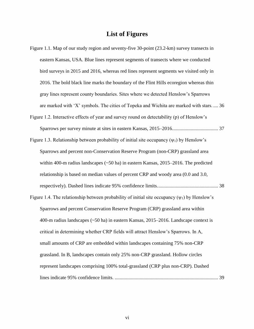
Figure 1.1. Map of our study region and seventy-five 30-point (23.2-km) survey transects in
eastern Kansas, USA. Blue lines represent segments of transects where we conducted
bird surveys in 2015 and 2016, whereas red lines represent segments we visited only in
2016. The bold black line marks the boundary of the Flint Hills ecoregion whereas thin
gray lines represent county boundaries. Sites where we detected Henslow’s Sparrows
are marked with ‘X’ symbols. The cities of Topeka and Wichita are marked with stars. .... 36
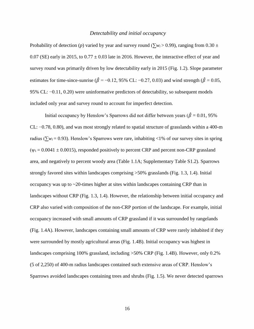
Figure 1.2. Interactive effects of year and survey round on detectability (p) of Henslow’s
Sparrows per survey minute at sites in eastern Kansas, 2015–2016. .................................... 37
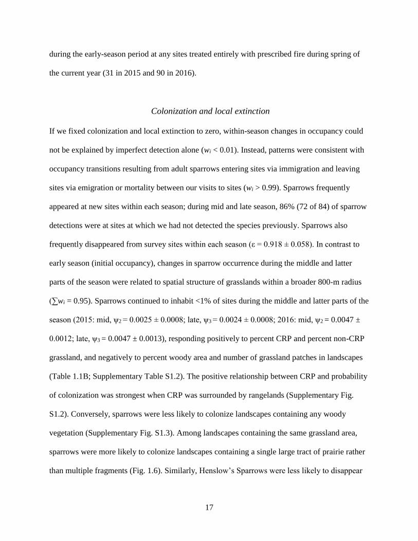
Figure 1.3. Relationship between probability of initial site occupancy (ψ1) by Henslow’s
Sparrows and percent non-Conservation Reserve Program (non-CRP) grassland area
within 400-m radius landscapes (~50 ha) in eastern Kansas, 2015–2016. The predicted
relationship is based on median values of percent CRP and woody area (0.0 and 3.0,
respectively). Dashed lines indicate 95% confidence limits. ................................................ 38
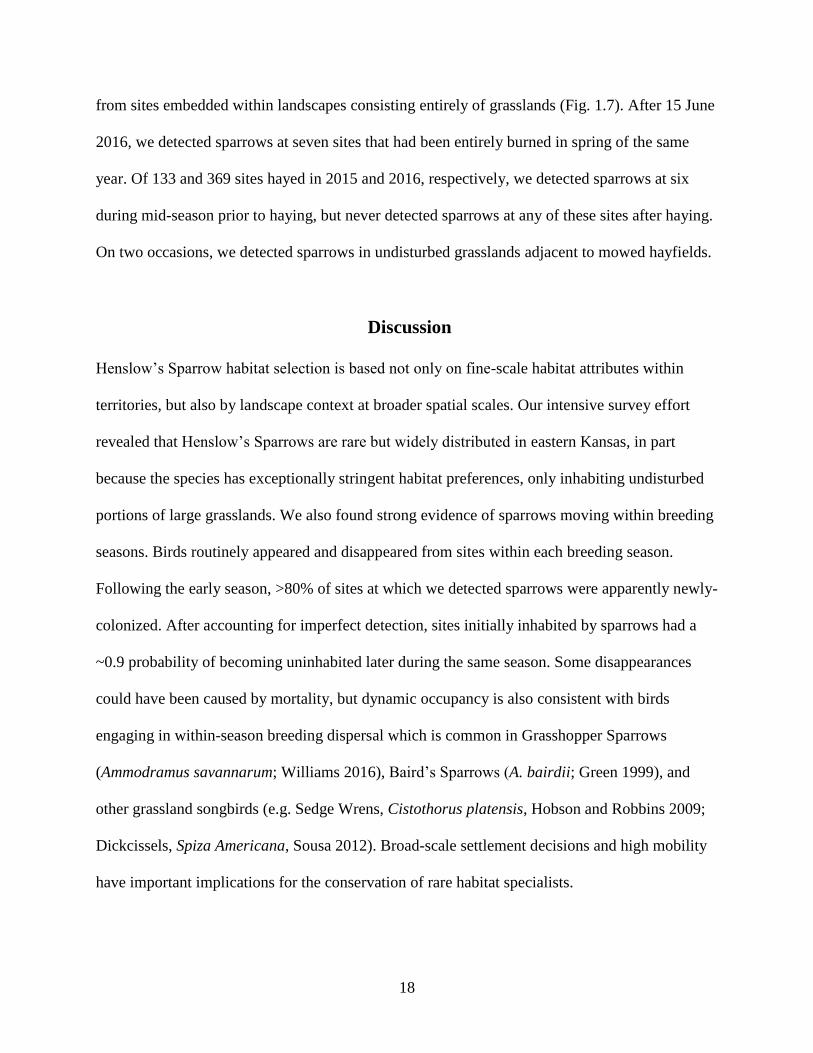
Figure 1.4. The relationship between probability of initial site occupancy (ψ1) by Henslow’s
Sparrows and percent Conservation Reserve Program (CRP) grassland area within
400-m radius landscapes (~50 ha) in eastern Kansas, 2015–2016. Landscape context is
critical in determining whether CRP fields will attract Henslow’s Sparrows. In A,
small amounts of CRP are embedded within landscapes containing 75% non-CRP
grassland. In B, landscapes contain only 25% non-CRP grassland. Hollow circles
represent landscapes comprising 100% total-grassland (CRP plus non-CRP). Dashed
lines indicate 95% confidence limits. ................................................................................... 39
vii
Figure 1.5. Relationship between percent woody area within 400-m radius landscapes (~50
ha) and initial site occupancy (ψ1) by Henslow’s Sparrows in eastern Kansas, 2015–
2016. Predictions are based on the median value of percent CRP area (0%). Dashed
lines indicate 95% confidence limits. ................................................................................... 40
Figure 1.6. The relationship between probability of site colonization (γ) by Henslow’s
Sparrows and percent non-CRP grassland within 800-m radius (~200 ha) landscapes
and in eastern Kansas, 2015–2016. Here, we show how the relationship between
colonization and non-CRP grassland varies when that grassland is distributed among
different numbers of patches. Probability of colonization was higher in 2016 and if the
same total grassland area was contained in a single patch versus several patches.
Predictions are based on median values of percent CRP and percent woody area (0%
and 5.1%, respectively). Dashed lines indicate 95% confidence limits. ............................... 41
Figure 1.7. Relationship between probability of within-season local extinction (ε) of
Henslow’s Sparrows and percent total grassland area (CRP plus non-CRP) within 800-
m radius (~200 ha) landscapes and in eastern Kansas, 2015–2016. Dashed lines
indicate 95% confidence limits. ............................................................................................ 42
Figure 2.1. Landscape change reduces total habitat area and can fragment contiguous habitat
into remnant patches of different shapes. We hypothesized that species abundance
could be driven by (A) total habitat area independent of patch configuration (the
number and shapes of patches within landscapes), or (B) core habitat area, which is
determined by both total habitat area and patch configuration. We also hypothesized
that abundance could also be driven by (C) quality of the landscape matrix. Hypotheses

viii
A and B are mutually exclusive, whereas neither A and C nor B and C are mutually
exclusive. .............................................................................................................................. 83
Figure 2.2. Map of our study region and seventy-five 30-point (23.2-km) survey transects in
eastern Kansas, USA. Blue lines represent segments of transects where we conducted
bird surveys in 2015 and 2016, whereas red lines represent segments we visited only in
2016. The bold black lines mark the boundaries of three major ecoregions in eastern
Kansas, whereas thin gray lines represent county boundaries. ............................................. 84
Figure 2.3. The relationship between probability of detection (p) of Grasshopper Sparrows
and (A) temperature and (B) wind strength in eastern Kansas, 2015−2016. Dotted lines
indicate 95% confidence limits. ............................................................................................ 85
Figure 2.4. The relationship between abundance (λ) of Grasshopper Sparrows per 150-m
radius (7 ha) site and core grassland area within 400-m radius (50 ha) landscapes in
eastern Kansas, 2015−2016. We plotted estimates of sparrow abundance over a range
of core grassland areas at three values of woody area to show how the relationship
between abundance and core grassland area is mediated by the amount of woody plants
in the surrounding matrix. From left to right, woody area values represent the
minimum, median, and 3rd quantile from our dataset. The curves in the middle and
right plots do not span the full range of core grassland area because part of these
landscapes contain woody area and abutting non-core grassland area. Dotted lines
indicate 95% confidence limits. ............................................................................................ 86
Figure 2.5. Abundance (λ) of Grasshopper Sparrows per 150-m radius (7 ha) site relative to
core grassland area (i.e. grasslands ≥60 m from edges) and woody area within 400-m
radius (50 ha) landscapes in eastern Kansas, 2015−2016. We present six site-specific
ix
estimates to show how sparrow abundance varied in landscapes containing the same
total grassland area. Dashed lines indicate the extent of survey sites. Light green, dark
green, and grey represent grassland, woodland, and other land-cover types (primarily
row-crop agriculture), respectively. Landscapes in columns A and B comprise 0 ha
woodland, whereas landscapes in column C comprise 5 ha (~10%) woodland. .................. 87
x
List of Tables
Table 1.1. Results of hierarchical model selection evaluating the effects of landscape factors
on the probabilities of initial site occupancy (ψ1) and within-season colonization (γ) for
Henslow’s Sparrows in eastern Kansas, 2015–2016. Subscript values indicate the
spatial scale (radius, in meters) associated with a given predictor variable. First, we
modeled variation in detectability (p), best explained by the function {Year × Survey
Round} (∑wi = 1.0), which we retained in subsequent models. Next, we estimated
initial occupancy. We retained the best-fitting model for initial occupancy (in italics)
and finished by estimating probabilities of colonization and local extinction (ε). We
estimated local extinction as a function of {Total Grass} at the same scale (i.e., 400,
800, or 1,600-m radius) used for estimating colonization in a given model. The lower
panel (final candidate set) includes all models from the top panel. Only models with wi
> 0.01 are shown. .................................................................................................................. 35
Table 2.1. Results of model selection evaluating the effects of landscape factors on
Grasshopper Sparrow detectability (p) and abundance (λ) in eastern Kansas, 2015–
2016. Squared superscripts (‘variable2’) indicate quadratic effects, whereas subscript
values indicate the spatial scale (radius, in meters) associated with a given predictor
variable. Latent abundance follows a zero-inflated Poisson distribution in all models
shown. Fifty-eight models with negligible support (wi < 0.01) are not shown. .................... 82
xi
List of Supplementary Figures
Figure S1.1. Relationships between percent total grassland area (CRP plus non-CRP) and
number of grassland patches (left column), and percent non-Conservation Reserve
Program (non-CRP) grassland area and number of non-CRP grassland patches (right
column), measured at three spatial scales (row A = 400-m radius, row B = 800-m
radius, and row C = 1600-m radius) centered on 2,249 survey points. Pearson
correlation coefficients (r) are indicated on each plot........................................................... 49
Figure S1.2. The relationship between site colonization (γ) by Henslow’s Sparrows and
percent Conservation Reserve Program (CRP) grassland area within 800-m radius
landscapes (~200 ha) in eastern Kansas, 2015–2016. In A, small amounts of CRP are
embedded within landscapes containing 75% non-CRP grasslands. In B, landscapes
containg only 25% non-CRP grassland. Hollow circles represent landscapes
comprising 100% total-grassland (CRP plus non-CRP). Dashed lines indicate 95%
confidence limits. .................................................................................................................. 50
Figure S1.3. Relationship between site colonization (γ) by Henslow’s Sparrows are percent
woody area within 800-m radius landscapes (~200 ha) in eastern Kansas, 2015–2016.
Predictions are based on median value of percent CRP area (0%). Grey and black and
lines represent 2015 and 2016, respectively. Dashed lines indicate 95% confidence
limits. .................................................................................................................................... 51
Figure S2.1. Relationship between total grassland area and core grassland area, measured
within 400-m radius (50 ha) landscapes centered around 2,249 unique survey points in
eastern Kansas. We provide Pearson correlation coefficients (r) across multiple ranges
of the dataset to show where total grassland area and core grassland area deviated from

xii
one another most (A: 25−35 ha or 50-70%; B: 20−40 ha or 40–80%; C: 0−50 ha or 0–
100%). ................................................................................................................................... 90
xiii
List of Supplementary Tables
Table S1.1. Summary statistics for unstandardized land cover data (TG = % total grassland
area, NCRP = % non-Conservation Reserve Program grassland area, CRP = %
Conservation Reserve Program grassland area, and NP = number of grassland patches)
used to model probabilities of initial site occupancy (ψ1), colonization (γ), and local
extinction (ε) for Henslow’s Sparrows in eastern Kansas, 2015–2016. We summarized
land-cover data within each of three spatial scales centered around 2,250 survey points.
In 2015, 31 of the 1,421 sites we surveyed were completely burned in spring and 133
were hayed. In 2016, 90 of the 2,250 sites were completely burned in spring and 369
were hayed. ........................................................................................................................... 47
Table S1.2. Slope parameter estimates (𝛽) and 95% confidence limits (LCL = lower
confidence limit, UCL = upper confidence limit) for the best-fitting model of initial
site occupancy (ψ1), local extinction (ε), site colonization (γ), and detectability (p) for
Henslow’s Sparrows in eastern Kansas, 2015–2016. Estimates are based on z-
transformed variables to facilitate comparisons.................................................................... 48
Table S2.1. Summary statistics for unstandardized land-cover data (Total Grass = total
grassland area, Core Grass = core grassland area, Woody = woody area) used to model
abundance (λ) of Grasshopper Sparrows in Eastern Kansas, 2015–2016. We
summarized land-cover data within each of four spatial scales centered on 2,249 survey
points. .................................................................................................................................... 88
Table S2.2. Slope parameter estimates (𝛽) and 95% confidence limits for our best-fit model
of Grasshopper Sparrow detectability (p) and abundance (λ) in eastern Kansas, 2015–
2016. Detectability and the zero-inflation factor (ψ) are on the logit scale, whereas

xiv
abundance is on the log scale. Estimates are based on z-transformed predictor
variables. ............................................................................................................................... 89
xv
Acknowledgements
I thank my field crew, Kevin Courtois, Pamela Moore, Lyndzee Rhine, Kevin Scott, Philip
Turner, and Eric Wilson, and lab assistant Suzy Replogle-Curnutt for their dedication and hard
work. My collaborator Michael Estey of the U.S. Fish and Wildlife Service provided logistical
and analytical support, and a valuable perspective toward my graduate research. Brian Meiwes
and Vickie Cikanek of Kansas Department of Wildlife, Parks and Tourism provided
accommodation for field crews at the Fall River Wildlife Area. My project was funded by the
U.S. Fish and Wildlife Service and Eastern Tallgrass Prairie and Big Rivers Landscape
Conservation Cooperative. The American Ornithologists’ Union, Friends of Sunset Zoo, and
Biology Graduate Students Association, College of Arts and Sciences, and Graduate Student
Council at Kansas State University provided funding that allowed me to attend regional,
national, and international conferences. I thank my major advisor, Dr. Alice Boyle for trusting
me to manage a region-wide study, and for motivating me to develop hypothesis-driven research
questions. My supervisory committee members, Dr. Kimberly With and Dr. Brett Sandercock
provided essential feedback that improved my work, while sparking my interests in landscape
ecology and population biology. I appreciate Virginia Winder for encouraging me to undertake a
Master of Science degree. I thank my lab mates, Sarah Winnicki, Emily Williams, Elsie Shogren,
and Carly Aulicky, and fellow graduate students Bram Verheijen and Eunbi Kwon for critiquing
my ideas, manuscripts, and presentations. I am grateful for the friendships I have formed here
with the people mentioned above, as well as John Kraft, Dan Sullins, Kirsten Grond, Amy
Berner, Lyla Hunt, Aaron Balogh, Kim O’Keefe, Eve McCulloch, Emily Weiser, Ryland Taylor,
Priscilla Moley, and John Shapel. Last, I thank Kate Waselkov for providing emotional support,
and for holding me up during the toughest periods of my graduate studies.

xvi
To my parents:
Conrad and Karen,
for encouraging my brother and me to pursue careers doing what we love.
1
Chapter 1 - Landscape context determines settlement patterns of an
enigmatic grassland songbird
Mark R. Herse1, Michael E. Estey2, Pamela J. Moore2, Brett K. Sandercock1, & W. Alice Boyle1
1Division of Biology, Kansas State University, Manhattan, Kansas, USA
2Habitat and Population Evaluation Team, U.S. Fish & Wildlife Service, Flint Hills National
Wildlife Refuge, Hartford, Kansas, USA
2
Abstract
Wildlife conservation requires an understanding of how landscape context influences habitat
selection at broader spatial scales than the home range. We aimed to assess how landscape
composition, fragmentation, and rangeland management affected occurrence and within-season
site-fidelity for a declining grassland songbird species, the Henslow’s Sparrow (Ammodramus
henslowii). Our study encompassed eastern Kansas (USA) and the largest remaining area of
tallgrass prairie (the Flint Hills ecoregion). We conducted 10,292 breeding-season point-count
surveys in 2015 and 2016, and related within-season site-occupancy dynamics of sparrows to
landscape factors at multiple spatial scales (400, 800, and 1,600-m radii). Henslow’s Sparrows
inhabited <1% of survey sites in eastern Kansas, often appearing at and disappearing from
survey sites within and between seasons. In spring, sparrows responded to landscape structure
most strongly at the 400-m radius scale, settling in areas containing >50% unburned prairie. In
summer, sparrows responded to landscape structure more strongly at the broader 800-m radius
scale, settling in areas containing >50% unfragmented prairie, including sites burned earlier the
same year. Sparrows were most likely to inhabit landscapes containing Conservation Reserve
Program (CRP) fields embedded within rangelands, disappeared from mowed hayfields, and
avoided landscapes containing trees. Landscape structure influenced habitat selection at spatial
scales far larger than that of an individual territory. Protecting prairie remnants from agricultural
conversion and woody encroachment, promoting CRP enrollment, and maintaining portions of
undisturbed prairie in working rangelands each year are critical to saving imperiled grassland
species. As habitat loss and fragmentation affects landscapes worldwide, effective conservation
will require ensuring conditions are suitable for at-risk species at multiple spatial scales.
Keywords: Flint Hills, habitat fragmentation, habitat loss, matrix effects, multiscale
3
Introduction
Animals select habitats by assessing the environment at multiple spatial scales and making a
series of hierarchical choices (Johnson 1980; Hutto 1985). Selection at each spatial scale can
influence individual fitness (Stamps 1994; Reed et al. 1999) and population viability (Pulliam
and Danielson 1991), and can vary over time as environmental conditions change (Block and
Brennan 1993). Broad-scale selection is reflected in a species’ geographic range and also in the
landscape features surrounding the home range, while fine-scale selection is represented by the
use of different microhabitats for foraging, reproduction, and shelter (Johnson 1980). Identifying
the physical attributes of habitats that animals choose allows wildlife managers to efficiently
allocate resources for species conservation (Blumstein and Fernández-Juricic 2004). For
example, assessing habitat choices over time can help predict sites where species are most likely
to settle, or subsequently disappear from, within and between breeding seasons (MacKenzie et al.
2006). However, most habitat studies focus on identifying correlates of fine-scale selection,
overlooking choices animals have already made at broader scales (Rolstad et al. 2000; Beasley et
al. 2007; Ciarniello et al. 2007).
Habitat destruction and land-use intensification are among the most serious
anthropogenic threats to wildlife populations globally (Tilman et al. 1994; Myers et al. 2000).
Grassland-dependent species are among the most endangered groups worldwide because most
native prairies have been converted to agricultural production (White et al. 2000). For example,
in North America, >96% of tallgrass prairies have been converted to row-crop agriculture during
the past two centuries (Samson and Knopf 1994). Consequently, many native grassland taxa
have experienced dramatic declines, including bison (Bison bison; Samson et al. 2004),
butterflies (Schlicht et al. 2009), and birds (Sauer et al. 2014). Grassland birds are of particular
4
concern, as populations of more than 20 common species have declined by >50% in the past 50
years (Butcher and Niven 2007), and about one-third of species are on the State of the Birds
Watch List (North American Bird Conservation Initiative 2016). Remaining tracts of tallgrass
prairie are critical to the long-term viability of grassland bird populations (With et al. 2008; U.S.
Fish and Wildlife Service 2010). Thus, information on habitat selection by grassland bird species
is urgently needed to guide conservation efforts aimed at protecting high-quality resources and
developing wildlife-friendly methods for managing agroecosystems (Askins et al. 2007).
The goal of our study was to assess the relative importance of landscape composition,
fragmentation, and rangeland management in driving habitat selection of an at-risk migratory
grassland songbird species, the Henslow’s Sparrow (Ammodramus henslowii). The species is
recognized as a bird of national conservation concern in the United States (Cooper 2012),
Endangered in Canada (COSEWIC 2011), and Near Threatened by the International Union for
Conservation of Nature (BirdLife International 2016). Identifying attributes of high-quality
habitats for Henslow’s Sparrows has been challenging because the species is rare, notoriously
elusive, and difficult to study. For nearly a century, Henslow’s Sparrows have been reported
appearing and disappearing from prairies within and between breeding seasons (Hyde 1939;
Wiens 1969; Ingold et al. 2009). Even at a regional scale, presence of Henslow’s Sparrows from
year to year is less predictable than other sympatric grassland sparrows (Dornak 2010, 2013).
However, most studies of Henslow’s Sparrows have focused on fine-scale habitat associations
within territories (e.g., Zimmerman 1988; Winter 1999; Monroe and Ritchison 2005). We have
limited information on how broad-scale landscape structure affects breeding habitat selection by
Henslow’s Sparrows (Bajema and Lima 2001; Cunningham and Johnson 2006; Jacobs et al.
2012), but such information might help to explain their sporadic patterns of occurrence. Thus, we
5
used multi-season occupancy models to relate within-season site-occupancy dynamics of
Henslow’s Sparrows to different landscape factors assayed at multiple spatial scales.
Methods
Study species
Henslow’s Sparrows have a male-territorial breeding system, and females nest in undisturbed
mesic grasslands characterized by tall native grasses and forbs, a dense litter layer, and abundant
standing dead vegetation (Zimmerman 1988; Herkert 1994). The species historically inhabited
large prairies, particularly in western portions of their breeding range in the Great Plains, where
natural selection could have favored innate preferences for habitat far from grassland edges
(Renfrew et al. 2005). Moreover, Henslow’s Sparrows may exhibit conspecific attraction,
preferring to congregate near one another (Vogel et al. 2011). Thus, rather than using all suitable
grasslands large enough to establish a single territory, sparrows may require a minimum area of
habitat that is larger than a territory (Ribic et al. 2009). Occurrence of Henslow’s Sparrows is
negatively associated with prescribed fire, grazing, and haying, which reduce vegetation height
and alter habitat suitability (Reinking 2005). Henslow’s Sparrows have benefited from
grasslands restored under the Conservation Reserve Program (CRP) because such prairies are not
prescribed fire or hayed, except in drought conditions (Herkert 2007). However, evidence for the
importance of CRP comes from regions dominated by row-crop agriculture, and it is unclear
whether sparrows favor CRP where large native prairies remain (Rahmig et al. 2009).
Suppression of ecological disturbance can also degrade prairies by promoting growth of woody
vegetation (Briggs et al. 2002). Like many grassland birds, Henslow’s Sparrows avoid grasslands
6
adjacent to woodlands (Winter et al. 2000; Patten et al. 2006), where nest predators tend to be
more abundant (Klug et al. 2010; Ellison et al. 2013).
We hypothesized that Henslow’s Sparrow habitat selection could be driven by (1)
availability of sufficient grassland area for territory establishment, (2) minimum area
requirements that are larger than a single territory, (3) prescribed fire and/or haying, or (4)
avoidance of nest predation. On average, Henslow’s Sparrow breeding territories are ~0.3–0.4 ha
in size (Monroe and Ritchison 2005; Jaster et al. 2013). Thus, if habitat selection is based solely
on the availability of sufficient grassland in which to establish a territory, we predicted that the
probability of sparrow occurrence would increase proportional to grassland area greater than ~1
ha. Alternatively, if habitat selection is driven by minimum area requirements, we predicted that
sparrows would only inhabit grassland areas that are larger than a territory. If vegetation
structure required for concealment drives habitat selection, we predicted that sparrows would
only inhabit grasslands undisturbed by fire for at least one growing season, and would disappear
from hayfields mowed during summer. If sparrows perceive restored grasslands to be suitable
breeding habitat, we predicted the probability of occurrence would be higher in areas containing
CRP than areas containing only grazed pastures. Last, assuming predators are more abundant
near woody areas and predation avoidance drives habitat selection, we predicated that among
areas containing the same amount of grassland habitat, sparrows would be more likely to inhabit
areas with fewer trees.
Study area and survey transects
Opportunities to study habitat selection by Henslow’s Sparrows in large grassland systems have
been limited because tallgrass prairies are now restricted to small remnants within agricultural
7
landscapes throughout most of North America (Samson et al. 2004). However, in the Flint Hills
ecoregion of eastern Kansas, shallow rocky soils are unsuitable for row-crop agriculture and
tallgrass prairie covers ~2 million ha (With et al. 2008). Past studies of Henslow’s Sparrows
within the Flint Hills have been limited to natural areas at Konza Prairie Biological Station
(Zimmerman 1988) and Fort Riley Military Reservation (Cully and Michaels 2000).
Our study area consisted of the eastern one-third of Kansas, which encompasses most of
the Flint Hills, parts of the Central Irregular Plains and Western Corn Belt Plains ecoregions
(Fig. 1.1; Omernik 1987), and essentially the entire breeding range of Henslow’s Sparrows in the
state. The Flint Hills is dominated by perennial warm-season grasses, which support an
economically-valuable grazing industry (With et al. 2008). More than 95% of the Flint Hills is
privately owned, and conservation must be carried out in partnership with private landowners in
working rangelands (U.S. Fish and Wildlife Service 2010). The Central Irregular Plains and
Western Corn Belt Plains are dominated by row-crop agriculture, but also contain fragmented
patches of warm and cool-season hayfields and pastures.
We conducted bird surveys along parts of existing North American Breeding Bird Survey
(BBS) routes, and a new set of transects established for this study (Fig. 1.1). The BBS is a long-
term citizen-science project in which observers conduct 3-min bird counts once per year during
the peak breeding season at points located along secondary roads throughout North America
(Sauer et al. 2014). Each BBS transect consists of 50 points spaced 800 m apart. Twenty-one
BBS transects occurred within our study area. We surveyed for birds at a subset of points along
each BBS transects to accommodate a longer survey duration while restricting all counts to
morning hours. We surveyed the first continuous segment of 25 points located (a) within our
study area and (b) outside of commercial, industrial, or residential areas, identified using
8
ArcMap 10.3 (Environmental Systems Research Institute, Redlands, CA). In addition, we created
thirty-six new 25-point transects following BBS protocols using a stratified random selection of
starting points (see Supplementary Text), for a total of 1,425 survey points located on fifty-seven
19.2-km transects in 2015. Following low detection rates in 2015, we increased the number of
points per transect and established additional transects. In 2016, we added five additional survey
points to all transects, and added eighteen new 30-point transects, for a total of 2,250 points
located on seventy-five 23.2-km transects (Fig. 1.1).
Field methods
We surveyed for Henslow’s Sparrows from their arrival in early spring until the end of the
breeding season. Each year, we conducted surveys in three ‘rounds.’ Start and end dates of
consecutive survey rounds sometimes overlapped by <1 week if heavy rains and poor road
conditions constrained survey schedules. We separated consecutive visits to the same transect by
at least two weeks. The start dates of each round were similar between years: ‘early season’
began 7 April in 2015 and 9 April in 2016, ‘mid season’ began 13 May in 2015 and 20 May in
2016, and ‘late season’ began 15 June in 2015 and 27 June in 2016. We completed all surveys on
23 July in 2015 and 29 July in 2016. We visited points in a consistent order beginning 30 min
before local sunrise and ending less than six hours after sunrise. We counted birds during dry
weather conditions when sustained wind speeds were ≤25 km/h. Each observer typically
completed one transect per morning, but if conditions deteriorated during the morning, we either
discarded data and re-visited the transect another day, or considered the transect to be complete if
the observer had conducted surveys at ≥20 points. Surveys were conducted by five observers in
2015 and four observers in 2016, with one observer shared between years (see Supplementary
9
Text). We rotated observers among transects during each round to minimize unmodeled
heterogeneity in our survey data (Mackenzie et al. 2003). We discarded data conducted by two
observers at 24 transects from the first round of 2015 due to concerns about possible species
misidentification.
At each survey point, the observer stood ~10 m from the vehicle and conducted a 6-min
survey using a modified version of the marsh bird monitoring protocol, which is designed to
detect cryptic species (Conway 2011). The observer mounted a bidirectional speaker (Veho,
Model VSS-009360BT; Dayton, OH, USA) on a tripod, oriented perpendicular to the road,
which broadcast a pre-recorded audio track. Surveys began with a 30-sec pre-survey period of
silence, and the audio track marked the beginning of each survey minute. During the first 30 sec
of mins 5 and 6, the audio track broadcast the song of a singing male Henslow’s Sparrow (~70
decibels at 0-m distance; recording from Missouri, Macaulay Library at the Cornell Lab of
Ornithology, catalog #38280) to elicit responses from nearby sparrows and to increase
probability of detection. Observers remained quiet and still during the pre-survey period so birds
could adjust to their presence, then recorded non-detections or detections of each individual
Henslow’s Sparrow seen or heard during each survey minute, recording the distance (m) and
cardinal direction to each individual at first detection. Observers measured distances to birds
using laser rangefinders (Nikon Prostaff 5; Melville, NY, USA) and estimated distances if they
could not see birds perched. For each survey, observers recorded the start time, wind strength
using the Beaufort Index, and mapped evidence of recent local fire or haying within our
maximum detection radius (250 m) on aerial photos.
10
Landscape factors and spatial scales
We obtained land-cover data developed by the Kansas Applied Remote Sensing Lab using
classified satellite imagery collected prior to 2005 (Peterson et al. 2010). Formal assessments of
overall accuracy for the base layer ranged from 76.5–86.2% (Peterson et al. 2010). We updated
the land-cover data by incorporating more detailed water bodies from the National Wetlands
Inventory digital database (U.S. Fish & Wildlife Service,
<https://www.fws.gov/wetlands/index.html>) and CRP enrollments as of 2012 (U.S. Department
of Agriculture, Farm Service Agency; proprietary data).
We summarized land-cover data within three spatial scales centered on each survey point
using ArcMap 10.3. We defined the most local scale as the area within a 400-m radius (51 ha) of
each survey point, which included our maximum detection radius (250 m). Henslow’s Sparrows
are thought to make settlement decisions at spatial scales larger than an individual territory
(Dornak 2010; Dornak et al. 2013), and adult males have been documented moving 1.6 km
between breeding attempts within the same breeding season in Missouri (A. Young, pers.
comm.). Thus, holding the resolution of land-cover data unchanged at a 30 m x 30 m raster pixel,
we doubled the spatial extent, quantifying attributes within 800 m (201 ha) and 1,600 m (804 ha)
radii of each survey point. The resulting range of spatial scales represent possible search areas
for Henslow’s Sparrows prospecting for sites to establish territories.
We considered seven landscape factors as potential sources of heterogeneity that could
influence occurrence of Henslow’s Sparrows. We pooled cool and warm-season grasslands
because the species breeds in both types (McCoy et al. 2001; Jaster et al. 2013). We classified
grasslands as (i) Conservation Reserve Program (CRP) grassland, (ii) non-CRP grassland, and
(iii) total grassland (CRP plus non-CRP). We then calculated the percent area for each type
11
within each scale. We included (iv) number of grassland patches (NP) as an index of
fragmentation, defined as the total number of unconnected patches of a given grassland type,
considering grassland pixels sharing either an edge (i.e. side) or corner to be connected. We
calculated (v) percent woody area based on land-cover classifications for which trees or shrubs
comprised >50% of the canopy (Peterson et al. 2010). We refer to the area surrounding each
survey point within our maximum detection radius (250 m) as ‘sites,’ and the area within each of
three spatial scales (400, 800, and 1,600-m radii) as ‘landscapes.’ We provide descriptive
statistics on local (vi) prescribed fire and (vii) haying at sites due to the importance of
management practices as drivers of vegetation structure (Bollinger 1995; Fuhlendorf et al. 2006).
Most prescribed fires were conducted in late winter or early spring before Henslow’s Sparrows
arrived on the breeding grounds. We categorized sites as completely burned if all grasslands
within a site had been burned during the current season, or unburned if grasslands were partially
burned or unburned. In eastern Kansas, haying usually begins in early June and continues
through July. In late summer, it was not always clear whether hayfields had been completely or
partially hayed; thus, we categorized sites as hayed if we observed any fields within a site to
have been mowed during the current season, or unhayed if pastures had not been cut.
Within-season site-occupancy dynamics
We used unconditional multi-season occupancy models to investigate within-season site-
occupancy dynamics of Henslow’s Sparrows (Mackenzie et al. 2003). We coded encounter
histories for bird surveys as follows. Observations of detection or non-detection occured at i = 1,
2, …, N sites during j = 1, 2, … kt secondary sampling occasions nested within t = 1, 2, …, T
primary sampling occasions. Investigators usually define entire breeding seasons as primary
12
sampling occasions and individual visits within seasons as secondary sampling occasions,
assuming that sites are ‘closed’ to individuals entering or leaving over each breeding season
(Mackenzie et al. 2003). The assumption of closure over an entire breeding season is often
unrealistic for birds, and if violated, can lead to biased estimates of model parameters (Rota et al.
2009). Thus, we defined our three rounds of surveys as primary sampling occasions, and
individual minutes within each survey as secondary sampling occasions. We combined detection
histories from 2015 and 2016 and considered each site to be independent between years (a)
because Henslow’s Sparrows are migratory and must make new habitat choices each breeding
season regardless of whether environmental conditions change, and (b) to maximize the
statistical power of our dataset (see Supplementary Text). We included year as a parameter to
test for inter-annual variation in sparrow abundance and potential observer effects.
Dynamic (i.e. multi-season) occupancy models estimate four parameters with maximum
likelihood. In our study, the closed part of the model estimated initial occupancy (ψ1), or the
probability a site was inhabited by at least one Henslow’s Sparrow during survey t = 1 (early
season), and detectability (pjt), or the probability an individual sparrow was detected if present
during min j of survey t. Non-detections could occur when sparrows were truly absent (1 – ψ), or
present but undetected (ψ × [1 – p]). Thus, the models did not assume sparrows were absent if
not detected. The open part of the model provides estimates of colonization (γ), or the probability
a site uninhabited during survey t became inhabited between t and t + 1, and local extinction (ε),
or the probability a site inhabited during survey t became uninhabited between t and t + 1.
Changes in occupancy (transitions) can occur between, but not during, primary sampling
occasions. Model parameter estimates pertain to our survey sites (defined by our 250-m detection
radius), quantified as a function of landscape features assayed at broader spatial scales
13
(summarized in Supplementary Table S1.1). We used linear models for all analyses because
quadratic and pseudo-threshold models did not provide better fits to our data during preliminary
analyses. We used a logit link to transform linear models to the probability scale (Mackenzie et
al. 2003). The dynamic occupancy models assumed that individual sparrows did not enter or
leave sites during our primary sampling occasions (i.e. 6-min survey). Additionally, these models
assume that observations of individuals were independent from one another, and sparrows were
not misidentified and recorded as present when absent. The assumptions were likely met because
the survey duration was short at 6 minutes, survey points were separated by 800 m, and we
trained field crews on species identification (see Supplementary Text).
Estimation of model parameters
We used a hierarchical approach to develop alternative models representing different
combinations of our a priori hypotheses. We compared models using an information-theoretical
approach (∆AICc and Akaike weights, wi), retaining top-fitting models following each step and
building upon them (Burnham and Anderson 2002). We considered models within 2.0 ∆AICc
units of the top model as competitive, and interpreted Akaike weights and sums of weights (∑wi)
as the relative likelihood of a model, or effects within multiple models, respectively, fitting our
data (Burnham and Anderson 2002). We dropped models that differed from the top model by one
parameter and ≤2.0 ∆AICc units if the estimated slope coefficients (�̂�) of predictor variables had
confidence intervals overlapping zero (Arnold 2010).
We z-transformed predictor variables prior to fitting models, and conducted analyses
using the ‘RMark’ package in R (Laake 2013; R Core Team 2016). Before modeling, we
assessed collinearity among all explanatory variables used together in any model. At
14
intermediate and broad spatial scales, percent total-grassland area and number of grassland
patches were related, as were percent non-CRP grassland area and number of non-CRP grassland
patches (800-m radius, r = 0.53–0.54; 1,600-m radius, r = 0.65–0.70). However, correlation was
largely driven by small numbers of patches in landscapes comprising small (<10%) or large
(>75%) amounts of grassland, with the number of patches varying widely in landscapes
containing intermediate amounts of grassland (Supplementary Fig. S1.1). We had a priori reason
to expect that fragmentation might help explain variation in occurrence of Henslow’s Sparrows
(Herkert et al. 2003; Ribic et al. 2009). Thus, we accepted some correlation among predictor
variables (0.53 < r < 0.70) in models that included effects of both grassland area and number of
grassland patches at intermediate and broad scales. Correlation among other variables used
together was low (r ≤ 0.31).
We first modeled temporal effects of our two years and three survey rounds on all
response parameters. We also considered ordinal date as an alternative temporal effect to survey
round. Moreover, we considered a model where colonization and local extinction were both set
to zero to test whether apparent within-season changes in occupancy could be explained entirely
by imperfect detection (Mackenzie et al. 2006). Next, we modeled effects of time-since-sunrise
and wind strength on detectability. After accounting for temporal effects and imperfect detection,
we determined how variation in landscape factors was associated with initial occupancy in two
steps. First, we tested whether Henslow’s Sparrows responded to percent total-grassland area, or
whether their response to grassland area was dependent on grassland type modeled as CRP
versus non-CRP. We also examined whether the relationship between percent grassland area and
sparrow occurrence varied with fragmentation, measured as number of grassland patches in
landscapes. Second, we added main effects of percent woody area at the spatial scale best fitting
15
our data in the previous step. We determined the association between landscape factors and
within-season occupancy dynamics using the same hierarchical approach described above for
initial occupancy. We only modeled effects of percent total-grassland area on local extinction
because we lacked statistical power to develop more complex models for this parameter. In
alternative models for transition parameters, we included total grassland area at the same spatial
scale used for estimating colonization. Goodness-of-fit procedures for estimating variance
inflation (�̂�) have not yet been developed for dynamic occupancy models. Therefore, we
conducted a post hoc sensitivity analysis of the final candidate model set to assess the robustness
of our inferences to potential sources of variance inflation (see Supplementary Text).
Results
Our results are based on data collected during 10,292 point-count surveys (3,656 surveys in 2015
and 6,636 in 2016). In 2015, we detected 34 Henslow’s Sparrows during 27 surveys at 27
different sites, never detecting sparrows at the same site more than once. In 2016, we detected
181 Henslow’s Sparrows during 103 surveys at 75 different sites. Of the 27 sites at which we
detected sparrows in 2015, we detected sparrows at only four sites in 2016. Of the 98 sites at
which we detected sparrows during the entire study, 75 sites had detections during only a single
visit (76.5% single-detection rate). Detections occurred evenly across the season in 2015 (nine
during each round), but increased as the season progressed in 2016 (early season, n = 22; mid
season, n = 38; late season, n = 43). Most of the 130 surveys with detections were of either a
single singing male (53%) or of two singing males (31%), whereas few were of three or more
males (16%).
16
Detectability and initial occupancy
Probability of detection (p) varied by year and survey round (∑wi > 0.99), ranging from 0.30 ±
0.07 (SE) early in 2015, to 0.77 ± 0.03 late in 2016. However, the interactive effect of year and
survey round was primarily driven by low detectability early in 2015 (Fig. 1.2). Slope parameter
estimates for time-since-sunrise (�̂� = −0.12, 95% CL: −0.27, 0.03) and wind strength (�̂� = 0.05,
95% CL: −0.11, 0.20) were uninformative predictors of detectability, so subsequent models
included only year and survey round to account for imperfect detection.
Initial occupancy by Henslow’s Sparrows did not differ between years (�̂� = 0.01, 95%
CL: −0.78, 0.80), and was most strongly related to spatial structure of grasslands within a 400-m
radius (∑wi = 0.93). Henslow’s Sparrows were rare, inhabiting <1% of our survey sites in spring
(ψ1 = 0.0041 ± 0.0015), responded positively to percent CRP and percent non-CRP grassland
area, and negatively to percent woody area (Table 1.1A; Supplementary Table S1.2). Sparrows
strongly favored sites within landscapes comprising >50% grasslands (Fig. 1.3, 1.4). Initial
occupancy was up to ~20-times higher at sites within landscapes containing CRP than in
landscapes without CRP (Fig. 1.3, 1.4). However, the relationship between initial occupancy and
CRP also varied with composition of the non-CRP portion of the landscape. For example, initial
occupancy increased with small amounts of CRP grassland if it was surrounded by rangelands
(Fig. 1.4A). However, landscapes containing small amounts of CRP were rarely inhabited if they
were surrounded by mostly agricultural areas (Fig. 1.4B). Initial occupancy was highest in
landscapes comprising 100% grassland, including >50% CRP (Fig. 1.4B). However, only 0.2%
(5 of 2,250) of 400-m radius landscapes contained such extensive areas of CRP. Henslow’s
Sparrows avoided landscapes containing trees and shrubs (Fig. 1.5). We never detected sparrows
17
during the early-season period at any sites treated entirely with prescribed fire during spring of
the current year (31 in 2015 and 90 in 2016).
Colonization and local extinction
If we fixed colonization and local extinction to zero, within-season changes in occupancy could
not be explained by imperfect detection alone (wi < 0.01). Instead, patterns were consistent with
occupancy transitions resulting from adult sparrows entering sites via immigration and leaving
sites via emigration or mortality between our visits to sites (wi > 0.99). Sparrows frequently
appeared at new sites within each season; during mid and late season, 86% (72 of 84) of sparrow
detections were at sites at which we had not detected the species previously. Sparrows also
frequently disappeared from survey sites within each season (ε = 0.918 ± 0.058). In contrast to
early season (initial occupancy), changes in sparrow occurrence during the middle and latter
parts of the season were related to spatial structure of grasslands within a broader 800-m radius
(∑wi = 0.95). Sparrows continued to inhabit <1% of sites during the middle and latter parts of the
season (2015: mid, ψ2 = 0.0025 ± 0.0008; late, ψ3 = 0.0024 ± 0.0008; 2016: mid, ψ2 = 0.0047 ±
0.0012; late, ψ3 = 0.0047 ± 0.0013), responding positively to percent CRP and percent non-CRP
grassland, and negatively to percent woody area and number of grassland patches in landscapes
(Table 1.1B; Supplementary Table S1.2). The positive relationship between CRP and probability
of colonization was strongest when CRP was surrounded by rangelands (Supplementary Fig.
S1.2). Conversely, sparrows were less likely to colonize landscapes containing any woody
vegetation (Supplementary Fig. S1.3). Among landscapes containing the same grassland area,
sparrows were more likely to colonize landscapes containing a single large tract of prairie rather
than multiple fragments (Fig. 1.6). Similarly, Henslow’s Sparrows were less likely to disappear
18
from sites embedded within landscapes consisting entirely of grasslands (Fig. 1.7). After 15 June
2016, we detected sparrows at seven sites that had been entirely burned in spring of the same
year. Of 133 and 369 sites hayed in 2015 and 2016, respectively, we detected sparrows at six
during mid-season prior to haying, but never detected sparrows at any of these sites after haying.
On two occasions, we detected sparrows in undisturbed grasslands adjacent to mowed hayfields.
Discussion
Henslow’s Sparrow habitat selection is based not only on fine-scale habitat attributes within
territories, but also by landscape context at broader spatial scales. Our intensive survey effort
revealed that Henslow’s Sparrows are rare but widely distributed in eastern Kansas, in part
because the species has exceptionally stringent habitat preferences, only inhabiting undisturbed
portions of large grasslands. We also found strong evidence of sparrows moving within breeding
seasons. Birds routinely appeared and disappeared from sites within each breeding season.
Following the early season, >80% of sites at which we detected sparrows were apparently newly-
colonized. After accounting for imperfect detection, sites initially inhabited by sparrows had a
~0.9 probability of becoming uninhabited later during the same season. Some disappearances
could have been caused by mortality, but dynamic occupancy is also consistent with birds
engaging in within-season breeding dispersal which is common in Grasshopper Sparrows
(Ammodramus savannarum; Williams 2016), Baird’s Sparrows (A. bairdii; Green 1999), and
other grassland songbirds (e.g. Sedge Wrens, Cistothorus platensis, Hobson and Robbins 2009;
Dickcissels, Spiza Americana, Sousa 2012). Broad-scale settlement decisions and high mobility
have important implications for the conservation of rare habitat specialists.
19
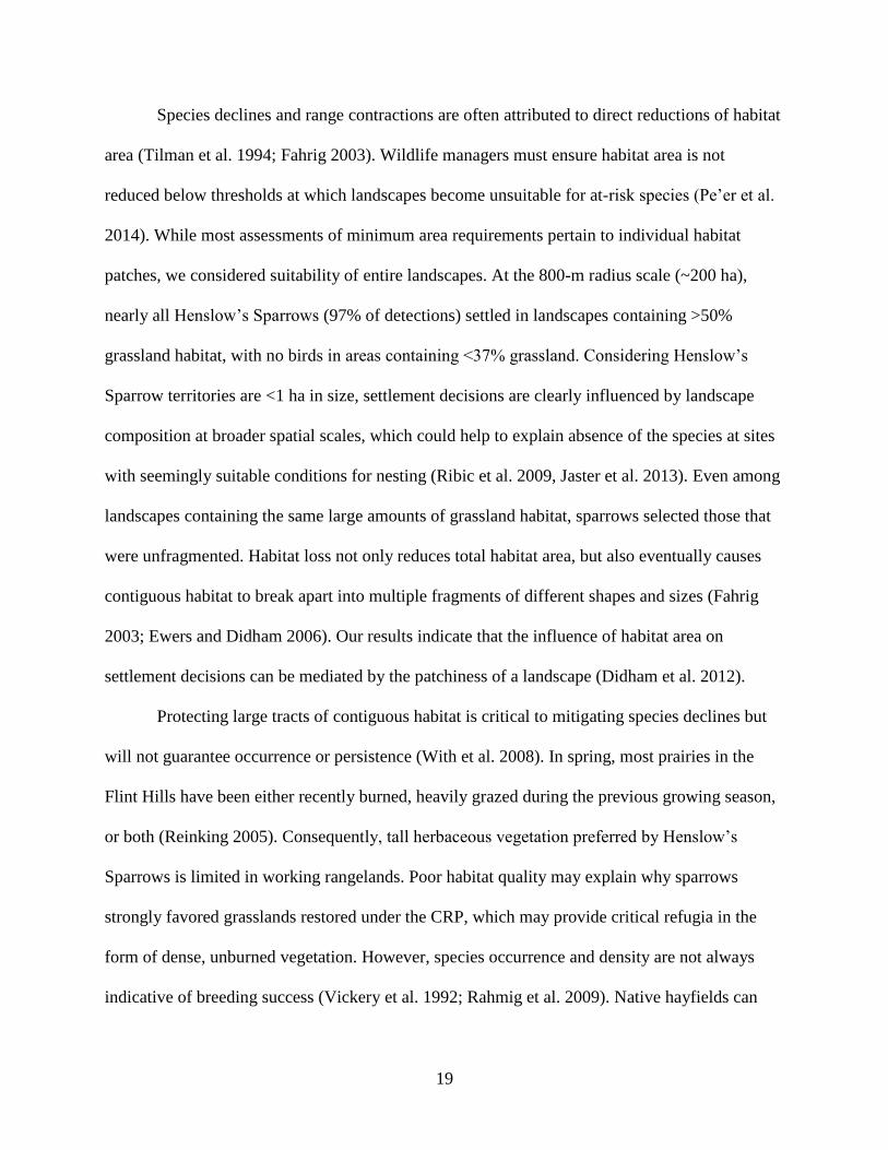
Species declines and range contractions are often attributed to direct reductions of habitat
area (Tilman et al. 1994; Fahrig 2003). Wildlife managers must ensure habitat area is not
reduced below thresholds at which landscapes become unsuitable for at-risk species (Pe’er et al.
2014). While most assessments of minimum area requirements pertain to individual habitat
patches, we considered suitability of entire landscapes. At the 800-m radius scale (~200 ha),
nearly all Henslow’s Sparrows (97% of detections) settled in landscapes containing >50%
grassland habitat, with no birds in areas containing <37% grassland. Considering Henslow’s
Sparrow territories are <1 ha in size, settlement decisions are clearly influenced by landscape
composition at broader spatial scales, which could help to explain absence of the species at sites
with seemingly suitable conditions for nesting (Ribic et al. 2009, Jaster et al. 2013). Even among
landscapes containing the same large amounts of grassland habitat, sparrows selected those that
were unfragmented. Habitat loss not only reduces total habitat area, but also eventually causes
contiguous habitat to break apart into multiple fragments of different shapes and sizes (Fahrig
2003; Ewers and Didham 2006). Our results indicate that the influence of habitat area on
settlement decisions can be mediated by the patchiness of a landscape (Didham et al. 2012).
Protecting large tracts of contiguous habitat is critical to mitigating species declines but
will not guarantee occurrence or persistence (With et al. 2008). In spring, most prairies in the
Flint Hills have been either recently burned, heavily grazed during the previous growing season,
or both (Reinking 2005). Consequently, tall herbaceous vegetation preferred by Henslow’s
Sparrows is limited in working rangelands. Poor habitat quality may explain why sparrows
strongly favored grasslands restored under the CRP, which may provide critical refugia in the
form of dense, unburned vegetation. However, species occurrence and density are not always
indicative of breeding success (Vickery et al. 1992; Rahmig et al. 2009). Native hayfields can
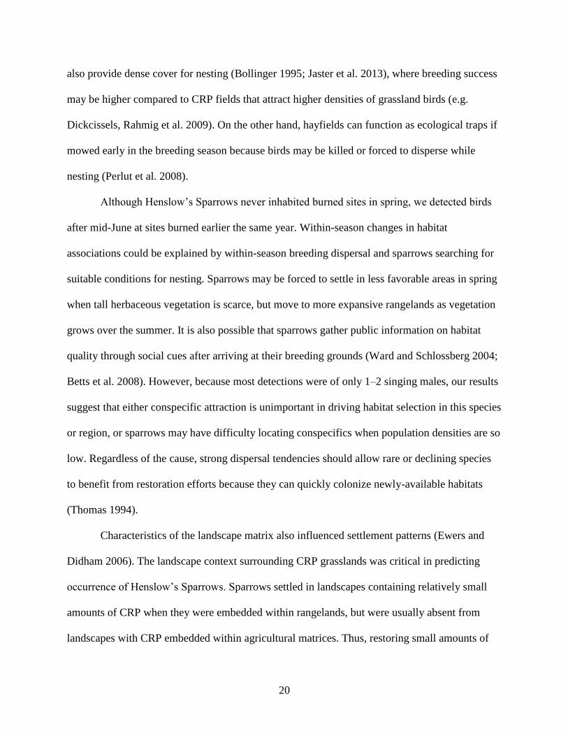
20
also provide dense cover for nesting (Bollinger 1995; Jaster et al. 2013), where breeding success
may be higher compared to CRP fields that attract higher densities of grassland birds (e.g.
Dickcissels, Rahmig et al. 2009). On the other hand, hayfields can function as ecological traps if
mowed early in the breeding season because birds may be killed or forced to disperse while
nesting (Perlut et al. 2008).
Although Henslow’s Sparrows never inhabited burned sites in spring, we detected birds
after mid-June at sites burned earlier the same year. Within-season changes in habitat
associations could be explained by within-season breeding dispersal and sparrows searching for
suitable conditions for nesting. Sparrows may be forced to settle in less favorable areas in spring
when tall herbaceous vegetation is scarce, but move to more expansive rangelands as vegetation
grows over the summer. It is also possible that sparrows gather public information on habitat
quality through social cues after arriving at their breeding grounds (Ward and Schlossberg 2004;
Betts et al. 2008). However, because most detections were of only 1–2 singing males, our results
suggest that either conspecific attraction is unimportant in driving habitat selection in this species
or region, or sparrows may have difficulty locating conspecifics when population densities are so
low. Regardless of the cause, strong dispersal tendencies should allow rare or declining species
to benefit from restoration efforts because they can quickly colonize newly-available habitats
(Thomas 1994).
Characteristics of the landscape matrix also influenced settlement patterns (Ewers and
Didham 2006). The landscape context surrounding CRP grasslands was critical in predicting
occurrence of Henslow’s Sparrows. Sparrows settled in landscapes containing relatively small
amounts of CRP when they were embedded within rangelands, but were usually absent from
landscapes with CRP embedded within agricultural matrices. Thus, restoring small amounts of
21
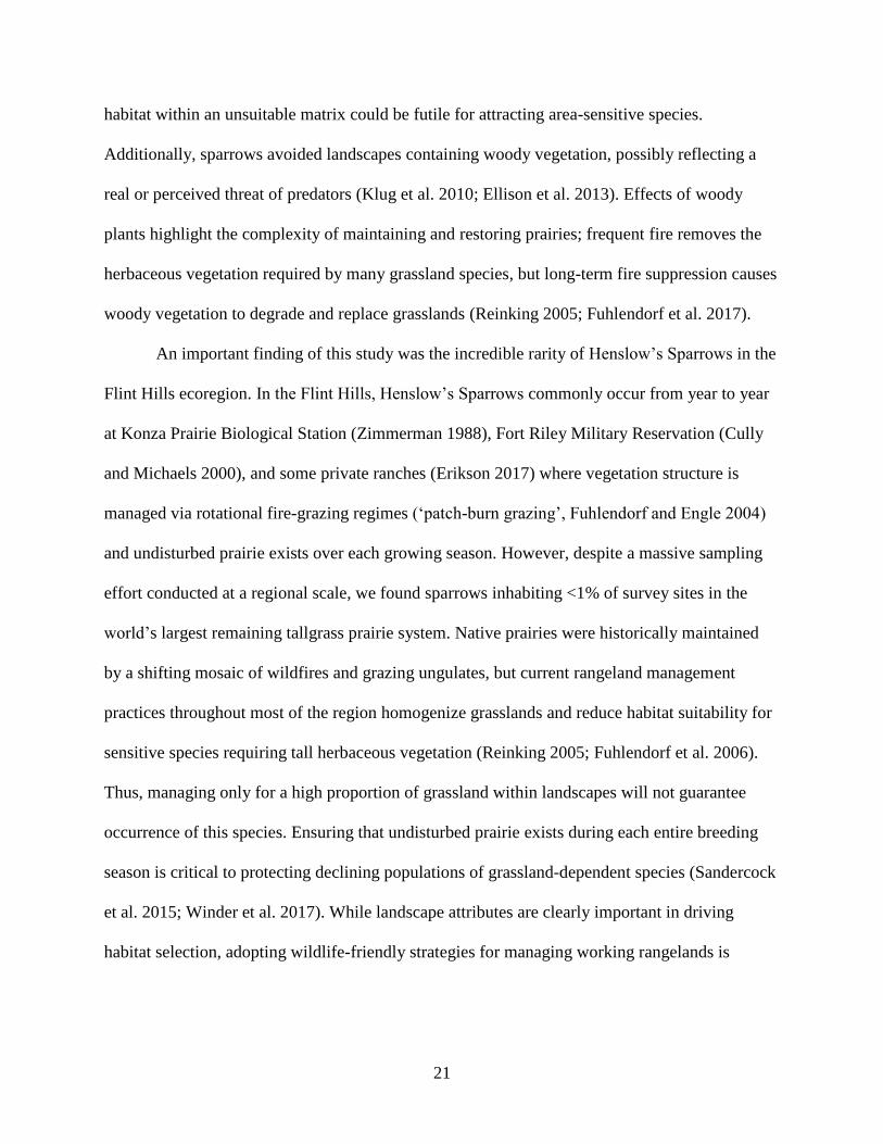
habitat within an unsuitable matrix could be futile for attracting area-sensitive species.
Additionally, sparrows avoided landscapes containing woody vegetation, possibly reflecting a
real or perceived threat of predators (Klug et al. 2010; Ellison et al. 2013). Effects of woody
plants highlight the complexity of maintaining and restoring prairies; frequent fire removes the
herbaceous vegetation required by many grassland species, but long-term fire suppression causes
woody vegetation to degrade and replace grasslands (Reinking 2005; Fuhlendorf et al. 2017).
An important finding of this study was the incredible rarity of Henslow’s Sparrows in the
Flint Hills ecoregion. In the Flint Hills, Henslow’s Sparrows commonly occur from year to year
at Konza Prairie Biological Station (Zimmerman 1988), Fort Riley Military Reservation (Cully
and Michaels 2000), and some private ranches (Erikson 2017) where vegetation structure is
managed via rotational fire-grazing regimes (‘patch-burn grazing’, Fuhlendorf and Engle 2004)
and undisturbed prairie exists over each growing season. However, despite a massive sampling
effort conducted at a regional scale, we found sparrows inhabiting <1% of survey sites in the
world’s largest remaining tallgrass prairie system. Native prairies were historically maintained
by a shifting mosaic of wildfires and grazing ungulates, but current rangeland management
practices throughout most of the region homogenize grasslands and reduce habitat suitability for
sensitive species requiring tall herbaceous vegetation (Reinking 2005; Fuhlendorf et al. 2006).
Thus, managing only for a high proportion of grassland within landscapes will not guarantee
occurrence of this species. Ensuring that undisturbed prairie exists during each entire breeding
season is critical to protecting declining populations of grassland-dependent species (Sandercock
et al. 2015; Winder et al. 2017). While landscape attributes are clearly important in driving
habitat selection, adopting wildlife-friendly strategies for managing working rangelands is
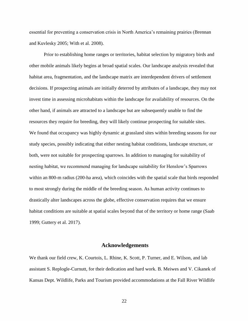
22
essential for preventing a conservation crisis in North America’s remaining prairies (Brennan
and Kuvlesky 2005; With et al. 2008).
Prior to establishing home ranges or territories, habitat selection by migratory birds and
other mobile animals likely begins at broad spatial scales. Our landscape analysis revealed that
habitat area, fragmentation, and the landscape matrix are interdependent drivers of settlement
decisions. If prospecting animals are initially deterred by attributes of a landscape, they may not
invest time in assessing microhabitats within the landscape for availability of resources. On the
other hand, if animals are attracted to a landscape but are subsequently unable to find the
resources they require for breeding, they will likely continue prospecting for suitable sites.
We found that occupancy was highly dynamic at grassland sites within breeding seasons for our
study species, possibly indicating that either nesting habitat conditions, landscape structure, or
both, were not suitable for prospecting sparrows. In addition to managing for suitability of
nesting habitat, we recommend managing for landscape suitability for Henslow’s Sparrows
within an 800-m radius (200-ha area), which coincides with the spatial scale that birds responded
to most strongly during the middle of the breeding season. As human activity continues to
drastically alter landscapes across the globe, effective conservation requires that we ensure
habitat conditions are suitable at spatial scales beyond that of the territory or home range (Saab
1999; Guttery et al. 2017).
Acknowledgements
We thank our field crew, K. Courtois, L. Rhine, K. Scott, P. Turner, and E. Wilson, and lab
assistant S. Replogle-Curnutt, for their dedication and hard work. B. Meiwes and V. Cikanek of
Kansas Dept. Wildlife, Parks and Tourism provided accommodations at the Fall River Wildlife

23
Area. K. A. With provided valuable comments that improved earlier versions of this chapter. Our
study is contribution no. 17-289-J from the Kansas Agricultural Experiment Station, and was
funded by U.S. Fish and Wildlife Service and Eastern Tallgrass Prairie and Big Rivers
Landscape Conservation Cooperative.
24
References
Arnold TW (2010) Uninformative parameters and model selection using Akaike’s information
criterion. J Wildl Manage 74:1175–1178
Askins RA, Chávez-Ramírez F, Dale BC, et al (2007) Conservation of grassland birds in North
America: understanding ecological processes in different regions. Ornithol Monogr 64:1–46
Bajema RA, Lima ST (2001) Landscape-level analyses of Henslow's Sparrow (Ammodramus
henslowii) abundance in reclaimed coal mine grasslands. Am Mid Nat 145:288–298
Beasley JC, Devault TL, Retamosa MI Jr (2007) A hierarchical analysis of habitat selection by
raccoons in northern Indiana. J Wildl Manage 71:1125–1133
Betts MG, Rodenhouse NL, Sillett TS, et al (2008) Dynamic occupancy models reveal within-
breeding season movement up a habitat quality gradient by a migratory songbird.
Ecography 31:592–600
Block W, Brennan LA (1993) The habitat concept in ornithology: theory and applications. Curr
Ornithol 11:35–91
Blumstein DT, Fernández-Juricic E (2004) The emergence of conservation behavior. Conserv
Biol 18:1175–1177
Bollinger EK (1995) Successional changes and habitat selection in hayfield bird communities.
Auk 112:720–730
Brennan LA, Kuvlesky WA Jr (2005) North American grassland birds: an unfolding
25
conservation crisis? J Wildlife Manage 69:1–13
Briggs J, Hoch G, Johnson L (2002) Assessing the rate, mechanisms, and consequences of the
conversion of tallgrass prairie to Juniperus virginianus forest. Ecosystems 5:578–586
Burnham K, Anderson D (2002) Model selection and multimodel inference: a practical
information-theoretic approach. Springer, New York, USA
Butcher GS, Niven DK (2007) Combining Data from the Christmas Bird Count and the Breeding
Bird Survey to Determine the Continental Status and Trends of North America Birds.
National Audubon Society, New York. Available from http://www.audubon.org/bird/
stateofthebirds/CBID/content/Report.pdf (accessed 3 Feb 2017)
Ciarniello L, Boyce M, Seip D, Heard D (2007) Grizzly bear habitat selection is scale dependent.
Ecol Appl 17:1424–1440
Conway CJ (2011) Standardized North American marsh bird monitoring protocol. 34:319–346
Cooper T (2012) Status Assessment and Conservation Plan for the Henslow’s Sparrow
(Ammodramus henslowii). U.S. Fish and Wildlife Service, Bloomington, Minnesota.
Available from https://www.fws.gov/midwest/es/soc/birds/pdf/
HESP_SAandConsPlan11Oct2012.pdf (accessed 12 Jan 2017)
Committee on the Status of Endangered Wildlife in Canada (2011) Assessment and Status
Report on the Henslow’s Sparrow Ammodramus henslowii in Canada, Ottawa, Ontario.
Available from http://www.registrelep-sararegistry.gc.ca/virtual_sara/files/cosewic/
sr_henslows_sparrow_0911_eng.pdf (accessed 12 Jan 2017)
26
Cully JF, Michaels HL (2000) Henslow’s Sparrow habitat associations on Kansas tallgrass
prairie. Wilson Bull 112:115–123
Cunningham MA, Johnson DH (2006) Proximate and landscape factors influence grassland bird
distributions. Ecol Appl 16:1062–1075
Didham RK, Kapos V, Ewers RM (2012) Rethinking the conceptual foundations of habitat
fragmentation research. Oikos 121:161–170
Dornak LL (2010) Breeding patterns of Henslow’s Sparrow and sympatric grassland sparrow
species. Wilson J Ornithol 122:635–645
Dornak LL, Barve N, Peterson A (2013) Spatial scaling of prevalence and population variation in
three grassland sparrows. Condor 115:186–197
Ellison KS, Ribic CA, Sample DW, et al (2013) Impacts of tree rows on grassland birds and
potential nest predators: a removal experiment. PLoS One 8:e59151
Erikson, AN (2017) Responses of grassland birds to patch-burn grazing in the Flint Hills of
Kansas. MS Thesis, Kansas State University, Manhattan, Kansas
Ewers RM, Didham RK (2006) Confounding factors in the detection of species responses to
habitat fragmentation. Biol Rev 81:117–142
Fahrig, L (2003) Effects of habitat fragmentation on biodiversity. Ann Rev Ecol Evol S 34:487–
515
27
Fuhlendorf SD, Engle DM (2004) Application of the fire-grazing interaction to restore a shifting
mosaic on tallgrass prairie. J Appl Ecol 41:604–614
Fuhlendorf SD, Harrell WC, Engle DM, et al (2006) Should heterogeneity be the basis for
conservation? Grassland bird response to fire and grazing. Ecol Appl 16:1706–1716
Fuhlendorf SD, Townsend DE III, Elmore RD, Engle DM (2010) Pyric-herbivory to promote
rangeland heterogeneity: evidence from small mammal communities. Rangel Ecol Manage
63:670–678
Fuhlendorf SD, Hovick TJ, Elmore RD, et al (2017) A hierarchical perspective to woody plant
encroachment for conservation of prairie-chickens. Rangel Ecol Manage 70:9–14
Green MT (1992) Adaptations of Baird's Sparrows (Ammodramus bairdii) to grasslands:
acoustic communication and nomadism. PhD Thesis, University of North Carolina, Chapel
Hill
Guttery MR, Ribic CA, Sample DW, et al (2017) Scale-specific habitat relationships influence
patch occupancy: defining neighborhoods to optimize the effectiveness of landscape-scale
grassland bird conservation. Landsc Ecol 32:515–529
Herkert JR (1994) Status and habitat selection of the Henslow’s Sparrow in Illinois. Wilson Bull
106:35–45
Herkert JR (2007) Conservation Reserve Program benefits on Henslow’s Sparrows within the
United States. J Wildl Manage 71:2749–2751
28
Herkert JR, Reinking DL, Wiedenfeld DA, et al (2003) Effects of prairie fragmentation on the
nest success of breeding birds in the midcontinental United States. Conserv Biol 17:587–
594
Hobson KA, Robbins MB (2009) Origins of late-breeding nomadic Sedge Wrens in North
America: limitation and potential hydrogen-isotope analyses of soft tissue. Condor
111:188–192
Hovick TJ, Miller JR, Dinsmore SJ, et al (2012) Effects of fire and grazing on Grasshopper
Sparrow nest survival. J Wildl Manag 76:19–27
Hutto RL (1985) Habitat selection by nonbreeding, migratory land birds. In: Cody M (ed)
Habitat selection in birds. Academic Press, Cambridge, UK
Hyde A (1939) The life history of Henslow’s Sparrow, Passerherbulus henslowii (Audubon).
University of Michigan Museum of Zoology Miscellaneous Publications 41
Ingold D, Dooley J, Cavender N (2009) Return rates of breeding Henslow’s Sparrows on mowed
versus unmowed areas on a reclaimed surface mine. Wilson J Ornithol 121:194–197
Jacobs RB, Thompson FR III, Koford RR, et al (2012) Habitat and landscape effects on
abundance of Missouri’s grassland birds. J Wildl Manage 76:372–381
Jaster L, Jensen WE, Forbes AR (2013) Abundance, territory sizes, and pairing success of male
Henslow’s Sparrows in restored warm- and cool-season grasslands. J Field Ornithol
84:234–241
29
Johnson DH (1980) The comparison of usage and availability measurements for evaluating
resource preference. Ecology 61:65–71
Klug PE, Jackrel SL, With KA (2010) Linking snake habitat use to nest predation risk in
grassland birds: the dangers of shrub cover. Oecologia 162: 803-813
Laake J (2013) RMark: An R Interface for Analysis of Capture-Recapture Data with MARK.
AFSC Processed Rep 2013-01, 25p. Alaska Fish Sci Cent, NOAA, Natl Mar Fish Serv,
Seattle
Mackenzie DI, Nichols JD, Hines JE, et al (2003) Estimating site occupancy, colonization, and
local extinction when a species is detected imperfectly. Ecology 84:2200–2207
Mackenzie DI, Nichols JD, Royle J, et al (2006) Occupancy Estimation and Modeling: Inferring
Patterns and Dynamics of Species Occurrence. Academic Press, San Diego, USA
McCoy T, Ryan MR, Burger LW Jr, Kurzejeski EW (2001) Grassland bird conservation: CP1 vs.
CP2 plantings in Conservation Reserve Program fields in Missouri. Am Midl Nat 145:1–17
Monroe MS, Ritchison G (2005) Breeding biology of Henslow’s Sparrows on reclaimed coal
mine grasslands in Kentucky. J Field Ornithol 76:143–149
Myers NC, et al (2000) Biodiversity hotspots for conservation priorities. Nature 403:853–858
North American Bird Conservation Initiative (2016) The State of North America's Birds 2016.
Environment and Climate Change Canada, Ottawa, Ontario. Available from
http://www.stateofthebirds.org/2016/wp-content/uploads/2016/05/SotB_16-04-26-english-
30
best.pdf (accessed 12 Jan 2017)
Omernik JM (1987) Ecoregions of the Conterminous United States. Ann Assoc Am Geogr
77:118–125
Pe'er G, Tsianou MA, Franz KW (2014) Toward better application of minimum area
requirements in conservation planning. Biol Conserv 170:92–102
Perlut NG, Strong AM, Donovan TM, Buckley NJ (2008) Grassland songbird survival and
recruitment in agricultural landscapes: implications for source–sink demography. Ecology
89:1941–1952
Peterson DL, Whistler J, Egbert SL, Martinko EA (2010) 2005 Kansas Land Cover Patterns
Phase II: Final Report. Kansas Biological Survey, University of Kansas, Lawrence.
Available from https://biosurvey.ku.edu/2005-kansas-land-cover-patterns-phase-ii-final-
report (accessed 12 Jan 2017)
Pulliam HR, Danielson BJ (1991) Sources, sinks, and habitat selection: a landscape perspective
on population dynamics. Am Nat 137:50–66
R Core Team (2016) R: A language and environment for statistical computing. R Foundation for
Statistical Computing, Vienna, Austria. Available from https://www.R-project.org (accessed
27 June 2017)
Rahmig CJ, Jensen WE, With KA (2009) Grassland bird responses to land management in the
largest remaining tallgrass prairie. Conserv Biol 23:420–432
31
Reed J, Bdulinier T, Danchin E, Dring L (1999) Informed dispersal: prospecting by birds for
breeding sites. Curr Ornithol 15:189–259
Reinking DL (2005) Fire regimes and avian responses in the central tallgrass prairie. Stud Avian
Biol 30:116–126
Renfrew RB, Ribic CA, Nack JL (2005) Edge avoidance by nesting grassland birds: a futile
strategy in a fragmented landscape. Auk 122:618–636
Ribic CA, Koford RR, Herkert JR, et al (2009) Area sensitivity in North American grassland
birds: patterns and processes. Auk 126:233–244
Ricketts AM, Sandercock BK (2016) Patch-burn grazing increases habitat heterogeneity and
biodiversity of small mammals in managed rangelands. Ecosphere 7:e01431
Rolstad J, Løken B, Rolstad E (2000) Habitat selection as a hierarchical spatial process: the
Green Woodpecker at the northern edge of its distribution range. Oecologia 124:116–129
Rota CT, Fletcher RJ, Dorazio RM, Betts MG (2009) Occupancy estimation and the closure
assumption. J Appl Ecol 46:1173–1181
Saab V (1999) Imporance of spatial scale to habitat use by breeding birds in riparian forests: a
hierarchical analysis. Ecol Appl 9:135–151
Samson FB, Knopf FL (1994) Prairie conservation in North America. Bioscience 44:418–421
Samson FB, Knopf FL, Ostlie WR (2004) Great Plains ecosystems: past, present, and future.
Wildlife Soc Bull 32:6–15
32
Sandercock BK, Alfaro-Barrios M, Casey AE, et al (2015) Effects of grazing and prescribed fire
on resource selection and nest survival of Upland Sandpipers in an experimental landscape.
Landsc Ecol 30:325–337
Sauer JR, Hines JE, Fallon JE, et al (2014) The North American Breeding Bird Survey, Results
and Analysis 1966–2013. United States Geological Survey Patuxent Wildlife Research
Center, Laurel, Maryland. Available from https://www.mbr-pwrc.usgs.gov/bbs/ (accessed
12 Jan 2017)
Schlicht D, Swengel A, Swengel S (2009) Meta-analysis of survey data to assess trends of prairie
butterflies in Minnesota, USA during 1979–2005. J Insect Conserv 13:429–447
Sousa BF (2012) Ecology of mating patterns and sexual selection in Dickcissels breeding in
managed prairie. PhD Thesis, University of Kentucky, Lexington, Kentucky
Stamps J (1994) Territorial behavior: testing the assumptions. Adv Study Behav 6:173–232
Swengel SR (1996) Management responses of three species of declining sparrows in tallgrass
prairie. Bird Conserv Int 6:241–253
Thomas CD (1994) Extinction, colonization, and metapopulations: environmental tracking by
rare species. Conserv Biol 8:373–378
Tilman D, May RM, Lehman CL, Nowak MA (1994) Habitat destruction and the extinction debt.
Nature 371:65–66
United States Fish and Wildlife Service (2010) Land Protection Plan: Flint Hill Legacy
33
Conservation Area. Flint Hills National Wildlife Refuge, Hartford, Kansas. Available from
https://www.fws.gov/refuge/flint_hills/partnerships/flint.html (accessed 12 Jan 2017)
Vogel JA, Koford RR, Otis DL (2011) Assessing the role of conspecific attraction in habitat
restoration for Henslow's Sparrows in Iowa. Prairie Nat 46:23–28
Ward MP, Schlossberg S (2004) Conspecific attraction and the conservation of territorial
songbirds. Conserv Biol 18:519–525
White R, Murray S, Rohweder M (2000) Pilot analysis of global ecosystems: grassland
ecosystems. World Resources Institute, Washington, DC. Available from
http://www.wri.org/sites/default/files/pdf/page_grasslands.pdf (accessed 12 Jan 2017)
Wiens (1969) An approach to the study of ecological relationships among grassland birds.
Ornithol Monogr 8:1–93
Williams, EJ (2016) Grasshopper Sparrows on the move: patterns and causes of within-season
breeding dispersal in a declining grassland songbird. MS Thesis, Kansas State University,
Manhattan, Kansas
Winder VL, McNew LB, Pitman JC, Sandercock BK (2017) Space use of female Greater Prairie-
Chickens in response to fire and grazing interactions. Rangel Ecol Manage 70:165–174
Winter M (1999) Nesting biology of Dickcissels and Henslow’s Sparrows in southwestern
Missouri prairie fragments. Wilson Bull 111:515–526
Winter M, Faaborg J (1999) Patterns of area sensitivity in grassland-nesting birds. Conserv Biol
34
13:1424–1436
Winter M, Johnson DH, Faaborg J (2000) Evidence for edge effects on multiple levels in
tallgrass prairie. Condor 102:256–266.
With KA, King AW, Jensen WE (2008) Remaining large grasslands may not be sufficient to
prevent grassland bird declines. Biol Conserv 141:3152–3167
Zimmerman JL (1988) Breeding-season habitat selection by the Henslow Sparrow
(Ammodramus henslowii) in Kansas. Wilson Bull 100:17–24
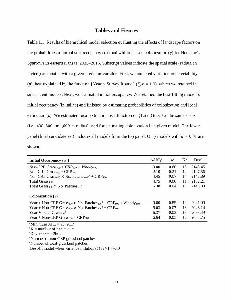
35
Tables and Figures
Table 1.1. Results of hierarchical model selection evaluating the effects of landscape factors on
the probabilities of initial site occupancy (ψ1) and within-season colonization (γ) for Henslow’s
Sparrows in eastern Kansas, 2015–2016. Subscript values indicate the spatial scale (radius, in
meters) associated with a given predictor variable. First, we modeled variation in detectability
(p), best explained by the function {Year × Survey Round} (∑wi = 1.0), which we retained in
subsequent models. Next, we estimated initial occupancy. We retained the best-fitting model for
initial occupancy (in italics) and finished by estimating probabilities of colonization and local
extinction (ε). We estimated local extinction as a function of {Total Grass} at the same scale
(i.e., 400, 800, or 1,600-m radius) used for estimating colonization in a given model. The lower
panel (final candidate set) includes all models from the top panel. Only models with wi > 0.01 are
shown.
Initial Occupancy (ψ1) ∆AICca wi Kb Devc
Non-CRP Grass400 + CRP400 + Woody400 0.00 0.60 13 2143.45
Non-CRP Grass400 + CRP400 2.10 0.21 12 2147.56
Non-CRP Grass400 × No. Patches400d + CRP400 4.45 0.07 14 2145.89
Total Grass400 4.75 0.06 11 2152.21
Total Grass400 × No. Patches400e 5.38 0.04 13 2148.83
Colonization (γ)
Year + Non-CRP Grass800 × No. Patches800d + CRP800 + Woody800 0.00 0.85 19 2041.09
Year + Non-CRP Grass800 × No. Patches800d + CRP800 5.03 0.07 18 2048.14
Year + Total Grass800f 6.37 0.03 15 2055.49
Year + Non-CRP Grass800 + CRP800 6.64 0.03 16 2053.75
aMinimum AICc = 2079.17 bK = number of parameters cDeviance = −2lnL dNumber of non-CRP grassland patches eNumber of total-grassland patches
fBest-fit model when variance inflation (�̂�) is ≥1.8–6.0
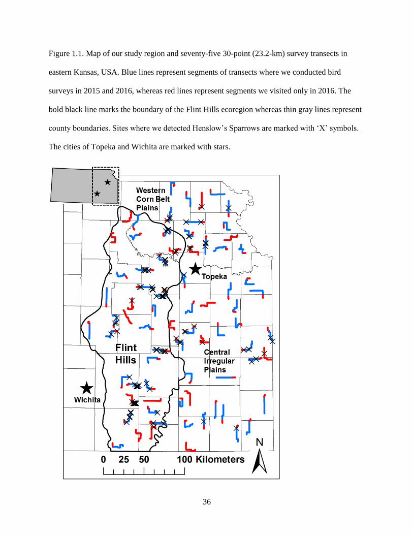
36
Figure 1.1. Map of our study region and seventy-five 30-point (23.2-km) survey transects in
eastern Kansas, USA. Blue lines represent segments of transects where we conducted bird
surveys in 2015 and 2016, whereas red lines represent segments we visited only in 2016. The
bold black line marks the boundary of the Flint Hills ecoregion whereas thin gray lines represent
county boundaries. Sites where we detected Henslow’s Sparrows are marked with ‘X’ symbols.
The cities of Topeka and Wichita are marked with stars.
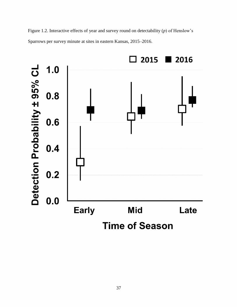
37
Figure 1.2. Interactive effects of year and survey round on detectability (p) of Henslow’s
Sparrows per survey minute at sites in eastern Kansas, 2015–2016.
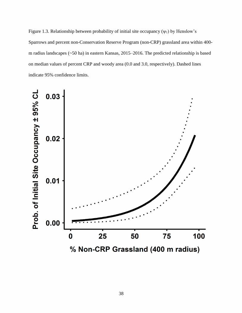
38
Figure 1.3. Relationship between probability of initial site occupancy (ψ1) by Henslow’s
Sparrows and percent non-Conservation Reserve Program (non-CRP) grassland area within 400-
m radius landscapes (~50 ha) in eastern Kansas, 2015–2016. The predicted relationship is based
on median values of percent CRP and woody area (0.0 and 3.0, respectively). Dashed lines
indicate 95% confidence limits.
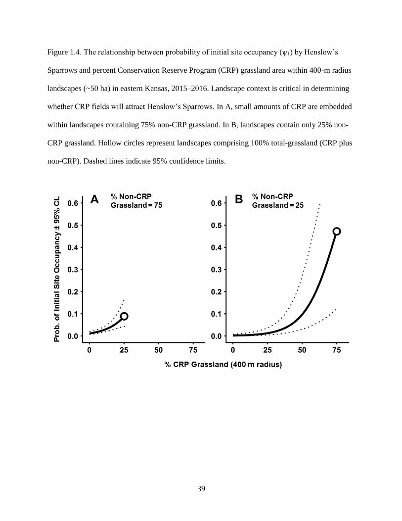
39
Figure 1.4. The relationship between probability of initial site occupancy (ψ1) by Henslow’s
Sparrows and percent Conservation Reserve Program (CRP) grassland area within 400-m radius
landscapes (~50 ha) in eastern Kansas, 2015–2016. Landscape context is critical in determining
whether CRP fields will attract Henslow’s Sparrows. In A, small amounts of CRP are embedded
within landscapes containing 75% non-CRP grassland. In B, landscapes contain only 25% non-
CRP grassland. Hollow circles represent landscapes comprising 100% total-grassland (CRP plus
non-CRP). Dashed lines indicate 95% confidence limits.
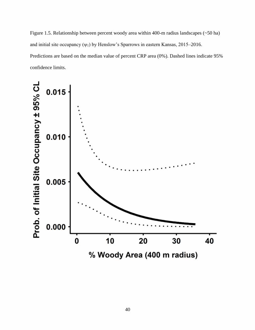
40
Figure 1.5. Relationship between percent woody area within 400-m radius landscapes (~50 ha)
and initial site occupancy (ψ1) by Henslow’s Sparrows in eastern Kansas, 2015–2016.
Predictions are based on the median value of percent CRP area (0%). Dashed lines indicate 95%
confidence limits.
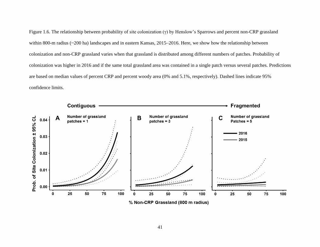
41
Figure 1.6. The relationship between probability of site colonization (γ) by Henslow’s Sparrows and percent non-CRP grassland
within 800-m radius (~200 ha) landscapes and in eastern Kansas, 2015–2016. Here, we show how the relationship between
colonization and non-CRP grassland varies when that grassland is distributed among different numbers of patches. Probability of
colonization was higher in 2016 and if the same total grassland area was contained in a single patch versus several patches. Predictions
are based on median values of percent CRP and percent woody area (0% and 5.1%, respectively). Dashed lines indicate 95%
confidence limits.
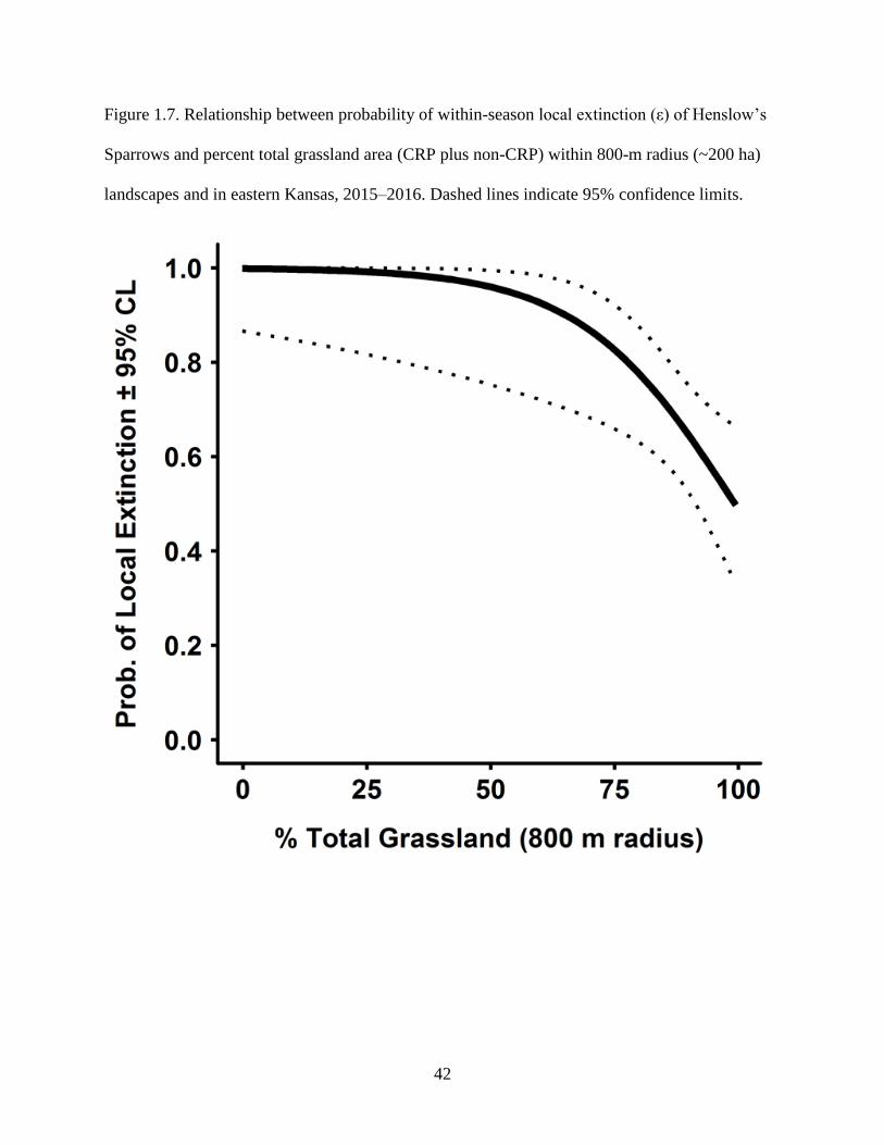
42
Figure 1.7. Relationship between probability of within-season local extinction (ε) of Henslow’s
Sparrows and percent total grassland area (CRP plus non-CRP) within 800-m radius (~200 ha)
landscapes and in eastern Kansas, 2015–2016. Dashed lines indicate 95% confidence limits.
43
Supplementary Text
Developing survey transects
We developed additional transects by stratifying our study area into thirty 1/4°-latitude by 1/4°-
longitude blocks, and identifying blocks within which BBS transects began. Following the same
general protocol used to establish BBS transects, we iteratively added random points to each
block until two starting locations (a new point or point 1 of an existing BBS transect) existed
within each block. We assigned only a single starting point to three blocks overlapping only a
small portion of our study area. We discarded random points within 8 km of a BBS point or
inside an urban area. We established new transects along secondary roads beginning from the
intersection closest to each random point. We constrained transects to avoid crossing state
boundaries, entering urban areas, or passing within 8 km of neighboring transects, but allowed
transects to cross block and ecoregion boundaries. Small segments of transects occasionally
occurred on paved roads when alternative routes did not exist, but we avoided such roads
whenever possible to minimize potential roadside bias. We created 36 new transects resulting in
1,425 total points located along fifty-seven 19.2-km transects in 2015. In 2016, we established
additional points to increase opportunities to encounter Henslow’s Sparrows. We conducted
surveys at five additional points along each existing BBS transect, and added five new points to
non-BBS transects. We also added an additional 30-point transect to each of 18 randomly
selected blocks, and reduced the minimum distance allowed between neighboring transects to 4
km, resulting in 2,250 total points located along seventy-five 23.2-km transects.
44
Observer training
We hired observers with previous birding experience. Prior to both field seasons, we trained
observers on use of laser rangefinders for recording distances to birds that were visible,
estimating distances to singing birds that were not visible, and identifying grassland birds by
sight and sound. We conducted mock surveys along transects to familiarize observers with
measuring distances and recording cardinal directions. We trained observers on identifying birds
in the field at Konza Prairie Biological Station, KS, and in the lab using Thayer Birding
Software. Prior to the 2016 field season, we also developed audio tracks that broadcast a variety
of singing grassland birds simultaneously. Some tracks included singing Henslow’s Sparrows
and some did not. We required observers to complete datasheets based on these recordings, and
did not begin our field season until all observers could positively identify all singing Henslow’s
Sparrows during the correct 1-minute intervals (without falsely identifying any birds). During
both years, M. Herse visited ≥2 transects as a secondary observer with each crew member during
each survey round (≥6 transects per observer per year) to ensure that observers remained
attentive and verifying identification skills over each season.
Pooling detection histories
We combined detection histories from 2015 and 2016, and considered each site to be
independent between years for five reasons. First, our primary goal was to understand how
landscape factors drive within-season site occupancy dynamics of Henslow’s Sparrows
independent of year effects. Second, among the sites we visited in both 2015 and 2016, history of
prescribed fire at 130 sites and haying at 292 sites was different between years. Third, we visited
825 sites only in 2016. Fourth, Henslow’s Sparrows have low site-fidelity (see Results), and
45
individuals returning during successive years to breed must make a new decision about whether
to inhabit a site, even if environmental conditions remain relatively unchanged. Fifth, our
analysis was based on a small number of detections, and combining study years allowed us to
maximize the statistical power of our dataset. We considered year effects in models to account
for potential differences in either Henslow’s Sparrow abundance, field crew capabilities, or both,
between years.
Meeting assumptions for multi-season occupancy models
In our study, models assume sites are closed to Henslow’s Sparrows entering or leaving during
primary sampling periods (i.e., surveys), observations of sparrows are independent from one
another, and sparrows were not falsely recorded when absent (Mackenzie et al. 2003). We met
the first assumption because our surveys were relatively brief and birds likely did not settle or
disperse away from sites while we were present. We met the second assumption because our
maximum detection radius for Henslow’s Sparrows was 250 m and adjacent survey points were
separated by 800 m; therefore, detecting the same individual bird during consecutive surveys on
a given day was highly unlikely. We avoided violating the third assumption by hiring
experienced observers with good birding skills, training less experienced observers on grassland
bird identification prior to each field season, and by omitting a subset of data from the early
season of 2015 (surveys conducted by two observers at 24 transects) which included possible
species misidentifications. We lacked enough detections per observer to consider potential
observer effects, but we rotated observers among transects, and potential differences in field
crew capabilities were also partially accounted for by a candidate year effect.
46
Sensitivity analysis
A common step in developing mark-recapture models is to assess the goodness-of-fit between
the most complex (global) model and detection histories by estimating a variation inflation factor
(�̂�), which is calculated by comparing between observed versus expected detection histories, and
adjusting model selection criteria to account for potential sources of overdispersion in the
dataset. When overdispersion does not exist, 𝑐 equals 1; however, �̂� values of >1–3 are not
uncommon in ecological data (MacKenzie et al. 2006). Formal tests for estimating �̂� do not yet
exist for multi-season occupancy models (Mackenzie et al. 2006). Rather than assuming
overdispersion was negligible in our dataset, we conducted a sensitivity analysis for our final
candidate set of models by adjusting �̂� from 1–6 and report changes in model rankings based on
Quasi-AICc (QAICc) rankings. Our approach provides a post hoc assessment of how robust our
dataset and inferences are to potential sources of overdispersion.
The best-fitting model in our final candidate set did not drop in rank until we increased
variance inflation (�̂�) above 1.8, and remained within 2.0 ∆QAICc units of the alternative top-
ranked model until we increased �̂� above 2.4. The simpler model that outcompeted others under
simulated conditions of high variance inflation was similar to the more complex model we
present, except that it only included main effects of year and percent total-grassland area on site
colonization (γ; Table 1B). The simpler model remained top-ranked when we increased �̂� to 6.0.
Most of the effects in the more complex model were retained during our sensitivity analysis, and
the effect that was relatively sensitive to variance inflation (interactive effect between percent
non-CRP grassland area and number of non-CRP grassland patches) was retained in the
parsimonious set even when �̂� was equal to 2.4. Thus, we consider our results robust to potential
sources of overdispersion commonly encountered in occupancy modeling.
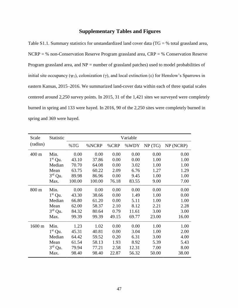
47
Supplementary Tables and Figures
Table S1.1. Summary statistics for unstandardized land cover data (TG = % total grassland area,
NCRP = % non-Conservation Reserve Program grassland area, CRP = % Conservation Reserve
Program grassland area, and NP = number of grassland patches) used to model probabilities of
initial site occupancy (ψ1), colonization (γ), and local extinction (ε) for Henslow’s Sparrows in
eastern Kansas, 2015–2016. We summarized land-cover data within each of three spatial scales
centered around 2,250 survey points. In 2015, 31 of the 1,421 sites we surveyed were completely
burned in spring and 133 were hayed. In 2016, 90 of the 2,250 sites were completely burned in
spring and 369 were hayed.
Scale Statistic Variable
(radius) %TG %NCRP %CRP %WDY NP (TG) NP (NCRP)
400 m
Min. 0.00 0.00 0.00 0.00 0.00 0.00
1st Qu. 43.10 37.86 0.00 0.00 1.00 1.00
Median 70.70 64.08 0.00 3.02 1.00 1.00
Mean 63.75 60.22 2.09 6.76 1.27 1.29
3rd Qu. 89.98 86.96 0.00 9.45 1.00 1.00
Max. 100.00 100.00 76.18 83.55 9.00 7.00
800 m
Min. 0.00 0.00 0.00 0.00 0.00 0.00
1st Qu. 43.30 38.66 0.00 1.49 1.00 0.00
Median 66.80 61.20 0.00 5.11 1.00 1.00
Mean 62.00 58.37 2.10 8.12 2.21 2.28
3rd Qu. 84.32 80.64 0.79 11.61 3.00 3.00
Max. 99.39 99.39 49.15 69.77 23.00 16.00
1600 m
Min. 1.23 1.02 0.00 0.00 1.00 1.00
1st Qu. 45.31 40.81 0.00 3.04 1.00 2.00
Median 64.42 59.52 0.20 6.31 3.00 4.00
Mean 61.54 58.13 1.93 8.92 5.39 5.43
3rd Qu. 79.94 77.21 2.58 12.31 7.00 8.00
Max. 98.40 98.40 22.87 56.32 50.00 38.00
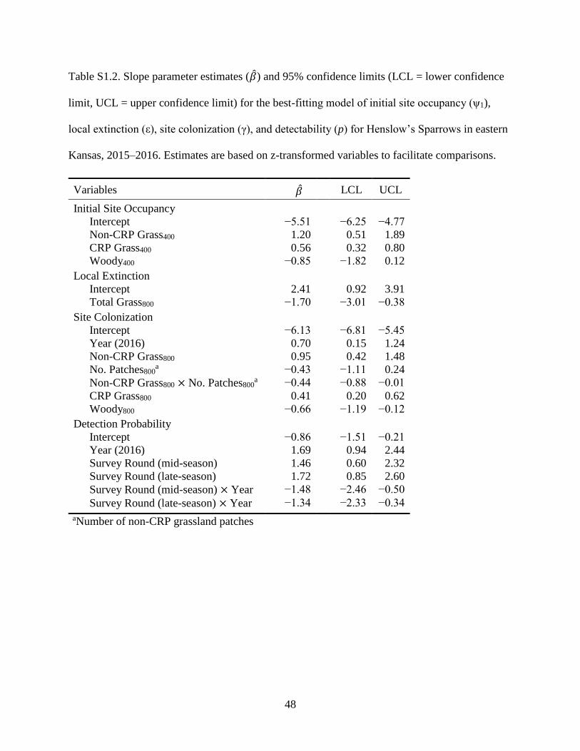
48
Table S1.2. Slope parameter estimates (�̂�) and 95% confidence limits (LCL = lower confidence
limit, UCL = upper confidence limit) for the best-fitting model of initial site occupancy (ψ1),
local extinction (ε), site colonization (γ), and detectability (p) for Henslow’s Sparrows in eastern
Kansas, 2015–2016. Estimates are based on z-transformed variables to facilitate comparisons.
Variables �̂� LCL UCL
Initial Site Occupancy
Intercept −5.51 −6.25 −4.77
Non-CRP Grass400 1.20 0.51 1.89
CRP Grass400 0.56 0.32 0.80
Woody400 −0.85 −1.82 0.12
Local Extinction
Intercept 2.41 0.92 3.91
Total Grass800 −1.70 −3.01 −0.38
Site Colonization
Intercept −6.13 −6.81 −5.45
Year (2016) 0.70 0.15 1.24
Non-CRP Grass800 0.95 0.42 1.48
No. Patches800a −0.43 −1.11 0.24
Non-CRP Grass800 × No. Patches800a −0.44 −0.88 −0.01
CRP Grass800 0.41 0.20 0.62
Woody800 −0.66 −1.19 −0.12
Detection Probability
Intercept −0.86 −1.51 −0.21
Year (2016) 1.69 0.94 2.44
Survey Round (mid-season) 1.46 0.60 2.32
Survey Round (late-season) 1.72 0.85 2.60
Survey Round (mid-season) × Year −1.48 −2.46 −0.50
Survey Round (late-season) × Year −1.34 −2.33 −0.34
aNumber of non-CRP grassland patches
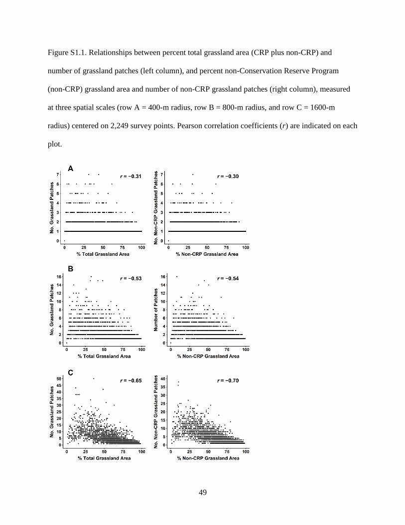
49
Figure S1.1. Relationships between percent total grassland area (CRP plus non-CRP) and
number of grassland patches (left column), and percent non-Conservation Reserve Program
(non-CRP) grassland area and number of non-CRP grassland patches (right column), measured
at three spatial scales (row A = 400-m radius, row B = 800-m radius, and row C = 1600-m
radius) centered on 2,249 survey points. Pearson correlation coefficients (r) are indicated on each
plot.
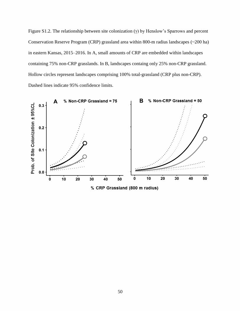
50
Figure S1.2. The relationship between site colonization (γ) by Henslow’s Sparrows and percent
Conservation Reserve Program (CRP) grassland area within 800-m radius landscapes (~200 ha)
in eastern Kansas, 2015–2016. In A, small amounts of CRP are embedded within landscapes
containing 75% non-CRP grasslands. In B, landscapes containg only 25% non-CRP grassland.
Hollow circles represent landscapes comprising 100% total-grassland (CRP plus non-CRP).
Dashed lines indicate 95% confidence limits.
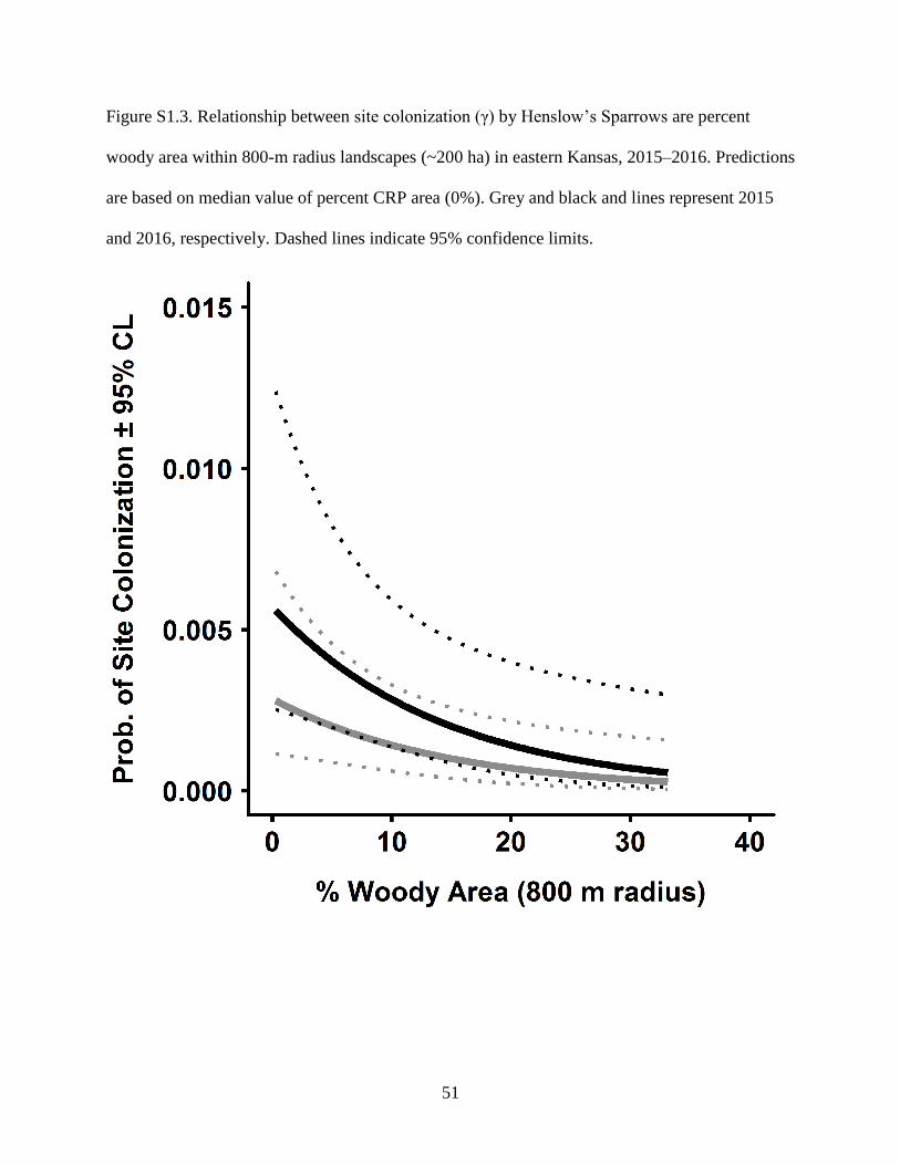
51
Figure S1.3. Relationship between site colonization (γ) by Henslow’s Sparrows are percent
woody area within 800-m radius landscapes (~200 ha) in eastern Kansas, 2015–2016. Predictions
are based on median value of percent CRP area (0%). Grey and black and lines represent 2015
and 2016, respectively. Dashed lines indicate 95% confidence limits.
52
Chapter 2 - The importance of core habitat versus total habitat
per se for a declining grassland songbird
Mark R. Herse1, Kimberly A. With1, & W. Alice Boyle1
1Division of Biology, Kansas State University, Manhattan, Kansas, USA
53
Abstract
Habitat loss and fragmentation (the spatial pattern of loss) are interdependent landscape-scale
processes. However, most fragmentation research is conducted at the patch scale and fails to
control for the amount of habitat in landscapes. Although direct reductions of habitat area may be
the main driver of species declines over the past two centuries, fragmentation could have
important indirect consequences. For example, fragmentation increases the edge-to-area ratio of
remnant habitat patches, reducing the amount of core habitat available to buffer sensitive species
from negative edge effects such as predation. Moreover, changes in the landscape matrix can
magnify negative edge effects, exacerbating the consequences of habitat loss and fragmentation.
However, the extent to which landscape attributes other than habitat area influence animal
populations is a topic of debate. Here, we tested whether abundance of a declining grassland
songbird, the Grasshopper Sparrow (Ammodramus savannarum), is driven by total habitat area
alone or by core habitat area, and whether abundance decreased as woody cover in the matrix
increased. We conducted 7,230 point-count surveys in 2015 and 2016 throughout eastern Kansas
(USA), home to the largest remaining tracts of tallgrass prairie in North America. We related
sparrow abundance to landscape structure assayed at multiple spatial scales (200, 400, 800, and
1600-m radii). Abundance was correlated most strongly with landscape structure within a 400-m
radius. Among landscapes containing the same total grassland area, sparrows favored those with
more core habitat and less woody cover. In landscapes with intermediate proportions of
grasslands (~50–70%), abundance decreased more than threefold if half the grassland area was
<60 m from an edge, and woody cover comprised 10% of the landscape. Thus, Grasshopper
Sparrow abundance was influenced more by core habitat than total habitat per se, which
underscores the importance of fragmentation and matrix quality in driving habitat selection. As

54
landscape change fragments habitat worldwide, conservation efforts focused on protecting and
restoring core habitat could help mitigate declines of sensitive species.
Keywords: edge effects, habitat fragmentation, landscape ecology, matrix effects, patch shape,
reserve design, woody encroachment
55
Introduction
Species extinctions and declines over the past two centuries have mainly been caused by habitat
destruction (Myers et al. 2000; Brook et al. 2003). Conversion of native habitat to other land uses
usually alters several aspects of landscape structure simultaneously, and it is often unclear which
alteration is most detrimental for declining species. Landscape change not only reduces the total
area that habitat covers, but can also fragment contiguous habitat into remnant patches of
different shapes and sizes (Prugh et al. 2008; Haddad et al. 2015). During the past half-century,
hundreds of studies have aimed to disentangle the relative influences of habitat area versus
fragmentation (the spatial arrangement or configuration of habitat) on species occurrence,
abundance, and richness (Fahrig 2003, 2017). However, disagreements over the role of habitat
fragmentation in driving species declines have sparked debate about the extent to which spatial
arrangements matter in conservation (With and Pavuk 2012; Fahrig 2013; Villard and Metzger
2014; Hanski 2015; Haddad et al. 2016).
Habitat area is important in determining availability of food and shelter, and therefore,
species occurrence, abundance, and richness (MacArthur and Wilson 1967; Wright 1983).
However, habitat area independent of fragmentation is often insufficient to explain how animal
populations respond to landscape change (With and King 2001; Ewers and Didham 2006;
Rybicki and Hanski 2013; With 2016). Fragmentation can influence habitat suitability directly
by increasing the number of smaller patches in landscapes or indirectly by increasing patch-
shape complexity and the amount of patch edge. Among landscapes containing the same amount
of habitat, different species may avoid or favor landscapes containing large proportions of edge
habitat, where predator-prey dynamics, interspecific competition, risk of parasitism, and/or
microclimate often differ from core habitats (Ries et al. 2004; Harper et al. 2005; Fletcher et al.
56
2007). Attributes of the landscape matrix surrounding natural areas can also influence animals’
perceptions of habitat quality, and consequently, habitat use by some species (Keyel et al. 2012;
Quesnelle et al. 2015).
Intrinsic differences in how animal populations respond to landscape structure can be
explained by species-level traits such as niche breadth and dispersal ability (Ewers and Didham
2006). However, conflicting conclusions regarding the consequences of landcape structure for
animal populations could also be explained by interdependence of habitat area and
fragmentation, such that the effect of habitat area is mediated by different patterns of
fragmentation such as patch shape or isolation (Didham et al. 2012; Wilson et al. 2016). Most
metrics used to characterize spatial arrangement in statistical models are designed to represent
only their direct, independent effects because correlations are considered a nuisance (McGarigal
and Cushman 2002; Fahrig 2003). However, if habitat area is correlated with fragmentation, then
part of an animal’s response to one factor is also an indirect response to the other (Ruffell et al.
2016). Thus, comparing only the direct effects of habitat area and fragmentation may
underestimate the importance of one or both factors. Conservationists cannot afford to wait for
new analytical tools or long-term field experiments to settle the ‘fragmentation debate’ (Villard
and Metzger 2014; Resasco et al. 2017), but must elucidate which landscape attributes influence
animal populations beyond habitat area (Didham et al. 2012).
As habitat is lost and becomes fragmented, an important attribute of remaining patches is
their shape (Ewers and Didham 2006). If patch shapes become highly convoluted, little or no
core area remains to buffer edge-sensitive species from the negative ecological consequences of
habitat edges such as increased predation (Laurance and Yensen 1991; Collinge 1996),
sometimes resulting in reduced population persistence (Bevers and Flather 1999; Cumming
57
2002). Many vertebrate species are not only edge-sensitive, but also area-sensitive in that they
only inhabit large habitat patches (Pe’er et al. 2014). However, patches containing the same total
area can vary in shape and therefore, core area. Theoretical models suggest that patch shape is an
important determinant of animal population size and viability in habitat remnants (Temple and
Cary 1988; Ewers and Didham 2007). However, empirical evidence for the importance of patch
shape is limited (Ewers and Didham 2006). Understanding the consequences of patch shape for
sensitive species requires sampling from numerous landscapes containing similar amounts of
habitat with different spatial arrangements, which are rare in the real world outside of
experimental model landscapes (With and Pavuk 2012; Villard and Metzger 2014).
Edge- and area-sensitivity are particularly common in bird species. Preferences for core
habitat by some species could be explained by lower reproductive success near edges, home
range requirements, or conspecific attraction (Robbins et al. 1989; Villard 1998; Ribic et al.
2009). Most evidence for the importance of patch shape in driving bird species occurrence or
abundance come from studies of forest birds (Robbins et al. 1989; Villard 1998; Ewers and
Didham 2006). However, little is known about the consequences of patch shape for grassland
birds. Many studies of grassland birds assess sensitivity of different species to total patch area or
size, but not patch shape or core area (Herkert 1994; Vickery and Herkert 2001; Ribic et al.
2009). Moreover, the data we do have on the importance of patch shape comes from patch-scale
studies conducted within clusters of prairie fragments (Helzer and Jelinksi 1999; Davis 2004;
Renfew and Ribic 2008). Temperate grasslands are a critically endangered biome because most
native prairies have been destroyed by agricultural expansion (Hoekstra et al. 2005). In North
America, >96% of native tallgrass prairie has been converted to row-crop agriculture during the
past two centuries (Samson and Knopf 1994). As a result, populations of >20 common grassland
58
bird species have declined by >50% during the past half-century (Butcher and Niven 2007), and
48% of species are of conservation concern (North American Bird Conservation Initiative 2016).
Knowledge of the consequences of patch shape for grassland birds is needed to guide
conservation efforts aimed at protecting and restoring native prairies in human-dominated
regions. Obtaining such information requires landscape-scale studies that assess bird abundance
across gradients of habitat fragmentation while controlling for habitat area (Fahrig 2017) and
accounting for the indirect effects of both factors (Ruffell et al. 2016).
Understanding the relative consequences of habitat area and fragmentation for sensitive
species is challenging because it typically requires large sample sizes, and sensitive species are
often rare (Henle et al. 2004) (see Chapter 1). We studied Grasshopper Sparrows (Ammodramus
savannarum) because the species is relatively common within remaining grasslands in the
eastern Great Plains, having broader habitat requirements than many other grassland-obligate
bird species (Vickery 1996), but has nevertheless experienced rangewide declines due to habitat
loss (Pardieck et al. 2016). We tested the following hypotheses; (a) sparrow abundance is driven
by habitat area alone (Fig. 2.1, hypothesis A); (b) the effect of habitat area on abundance of
sparrows is mediated by patch shape (Fig. 2.1, hypothesis B); and/or (c) matrix quality
influences the abundance of sparrows (Fig. 2.1, hypothesis C). We distinguished between
hypotheses A and B by determining whether total habitat area or core habitat area better
explained variation in sparrow abundance. Core habitat area is an integrative metric determined
by both habitat area, patch shape, and a species-specific edge avoidance threshold (McGarigal et
al. 2012), and therefore retains the direct and indirect effects of both habitat area and
configuration. This ecologically-scaled metric improves upon neutral landscape metrics in that it
is based on both species and landscape attributes rather than only the latter (Vos et al. 2001). To
59
test the hypothesis that matrix quality influences sparrow abundance, we focused on the amount
of woody cover in landscapes. Like many grassland bird species, Grasshopper Sparrows avoid
grasslands adjacent to woodlands (Johnson and Temple 1990; Renfrew et al. 2005), where
predators are often more abundant and nest-predation rates are highest (Klug et al. 2010; Ellison
et al. 2013). Thus, if risk of predation drives habitat selection, we predicted that among
landscapes containing the same total grassland area, sparrow abundance would be negatively
associated with the amount of trees and shrubs in the surrounding matrix. We distinguished
between these alternatives by using hierarchical N-mixture models to relate sparrow abundance
to landscape factors assayed at multiple spatial scales centered on thousands of survey points
located in eastern Kansas, home to North America’s largest remaining tracts of tallgrass prairie.
Methods
Study species
Grasshopper Sparrows historically inhabited large expanses of prairies in western portions of
their breeding range in the Great Plains (Vickery 1996) where natural selection could have
favored innate preferences for grassland habitat that is far from edges (Renfrew et al. 2005). The
species has a male-territorial breeding system, and nests in a variety of arid and mesic grasslands
characterized by moderate vegetative cover (Vickery 1996). Sparrow abundance and nest
densities are decreased within ~50 m of croplands or woodlands (Johnson and Temple 1990,
Delisle and Savidge 1996, Renfrew et al. 2005, Patten et al. 2006). Moreover, sparrows
sometimes exhibit conspecific attraction in that territorial males prefer to congregate near one
another (Andrews et al. 2015). Thus, rather than using all suitable grasslands with sufficient area
60
for establishing a single territory, sparrows may require a minimum area of core habitat far from
edges or sufficient to accommodate multiple territories (Ribic et al. 2009).
Study area and survey transects
More than 80% (~2 million ha) of the tallgrass prairie remaining in North America is located in
the Flint Hills ecoregion of Kansas and Oklahoma (USA) where shallow rocky soils are
unsuitable for tilling (With et al. 2008). Our study area consisted of the eastern one-third of
Kansas, encompassing almost all of the Flint Hills ecoregion, and parts of the adjacent Central
Irregular Plains and Western Corn Belt Plains ecoregions (Fig. 2.2; Omernik 1987). The Flint
Hills is dominated by perennial warm-season grasses which support a major cattle industry (With
et al. 2008). The main land-use in the Central Irregular Plains and Western Corn Belt Plains is
row-crop agriculture, but both regions also contain fragmented hayfields and pastures. The
region provides an excellent opportunity to assess the influence of landscape structure on species
abundance because within local areas, percent grassland ranges from 0−100%, and is configured
in a variety of spatial arrangements.
We conducted bird surveys along existing North American Breeding Bird Survey (BBS)
routes and new transects that we established (Fig. 2.2; see Chapter 1). The BBS is a long-term
citizen-science project in which observers conduct 3-min bird counts once per year during the
breeding season at points located along secondary roads throughout the USA (Sauer et al. 2014).
Each transect consists of 50 points spaced 800 m apart. Twenty-one BBS transects were located
within our study region. We surveyed for birds at a subset of points along each BBS transect to
accommodate a longer survey duration while restricting all counts to morning hours. We
surveyed the first continuous segment of 25 points located (a) within our study area and (b)
61
outside of commercial, industrial, or residential areas identified using ArcMap 10.3
(Environmental Systems Research Institute, Redlands, CA). We created thirty-six 25-point
transects following BBS protocols using a stratified random selection of starting points, for a
total of 1,425 survey points located on fifty-seven 19.2-km transects in 2015. To increase
detections in 2016, we added five new survey points to all transects, and added eighteen 30-point
transects, for a total of 2,250 survey points located on seventy-five 23.2-km transects (Fig. 2.2).
Field methods
We surveyed for Grasshopper Sparrows from approximately one month following their arrival in
mid-April until the end of the breeding season in late July. Each year, we conducted surveys in
two ‘rounds.’ Start and end dates of survey rounds overlapped by <1 week in 2015 due to heavy
rains and poor road conditions which constrained survey schedules. We separated consecutive
visits to the same transect by at least two weeks. The start dates of each round were similar
between years: ‘Round 1’ began 13 May in 2015 and 20 May in 2016, and ‘Round 2’ began 15
June in 2015 and 27 June in 2016. All surveys in Round 2 ended by 23 July in 2015 and 29 July
in 2016. We visited points in a consistent order beginning 30 min before local sunrise and ending
less than six hours after sunrise. We counted birds during days with little or no rainfall when
sustained wind speeds were ≤25 km/h. We recorded the start time, temperature (°C), and wind
strength using the Beaufort Index at the beginning of each bird survey. Each observer typically
completed one transect per morning, but if conditions deteriorated during the morning, we either
discarded data and re-visited the transect another day, or considered the transect to be complete if
the observer had conducted surveys at ≥20 points. Surveys were conducted by five observers in
2015 and four observers in 2016, with one observer shared between years. We rotated observers
62
among transects during each round to minimize unmodeled heterogeneity in our survey data
(Mackenzie and Royle 2005).
At each survey point, the observer stood ~10 m from the vehicle and conducted a 6-min
point count. Observers remained quiet and still during a 30-sec pre-survey period so birds could
adjust to their presence, then recorded detections of individual Grasshopper Sparrows seen or
heard, recording the distance (m) and cardinal direction to each individual at first detection.
Observers measured distances to birds using laser rangefinders (Nikon Prostaff 5; Melville, NY,
USA) and estimated distances if they could not see birds perched. As part of a separate study
(see Chapter 1), the observer broadcast a 30-sec pre-recorded song of a singing male Henslow’s
Sparrow (~70 decibels at 0-m distance) from a bidirectional speaker (Veho, Model VSS-
009360BT; Dayton, OH, USA) during each of the final two minutes of each survey. Grasshopper
Sparrows were not noticeably deterred nor attracted by the broadcast, and often continued
singing or remained perched on roadside fences during the broadcast (M. Herse, pers. observ.).
Landscape factors and spatial scales
We obtained land-cover data developed by the Kansas Applied Remote Sensing Lab using
classified satellite imagery collected prior to 2005 (Peterson et al. 2010). Formal assessments of
overall accuracy for the base layer range from 76.5–86.2% (Peterson et al. 2010). We
summarized land-cover data at spatial scales relevant to the dispersal behavior of Grasshopper
Sparrows (Wheatley and Johnson 2009). Within-season breeding dispersal distances of male
Grasshopper Sparrows in eastern Kansas are large relative to their ~0.5-ha territories (median
dispersal distance = 197 m, mean = 695 m, range: 101–8940 m, n = 213 sparrows; Williams
2016). Being migratory with low site fidelity in this region (<20% adult male return rate; W. A.
63
Boyle, unpublished data), sparrows likely prospect for suitable breeding sites over even larger
distances between years. We summarized land-cover data within four spatial scales centered on
each survey point using ArcMap 10.3 and Fragstats 4.2 (McGarigal et al. 2012). We defined the
most local scale as the area within a 200-m radius (13 ha) around each survey point, which
corresponds with the median of within-season dispersal distances (Williams 2016). Then,
holding the resolution of land-cover data unchanged at a 30 m x 30 m raster pixel, we doubled
the radius and summarized spatial data within 400-m (51 ha), 800-m (201 ha), and 1600-m (804
ha) radii of each survey point. The resulting range of spatial scales represent potential search
areas for sparrows prospecting for suitable habitat.
We considered three landscape factors as potential sources of variation in sparrow
abundance (Fig. 2.1). We classified grassland as (i) total grassland area and (ii) core grassland
area. We defined core grassland area as grasslands ≥60 m from woodlands, croplands,
waterbodies, or urban areas (commercial, industrial, or residential). We selected this buffer based
on documented edge-avoidance within ~50 m of edges between grasslands and croplands or
woodlands (Johnson and Temple 1990, Delisle and Savidge 1996, Renfrew et al. 2005, Patten et
al. 2006). We increased the buffer to 60 m due to our use of 30-m wide raster pixels. If the
relationship between sparrow abundance and habitat area is mediated by patch shape and the
amount of edge in landscapes, we predicted that core grassland area would explain more
variation in sparrow abundance than total habitat area. We then calculated the area of each
grassland type (ha) within each scale. Overall, at the same spatial scales, total and core grassland
area were closely related (0.93 < r < 0.97). However, the two factors were less related in
landscapes containing intermediate proportions of grassland cover. For example, at the 400-m
radius scale, correlation was much lower in landscapes comprising 50–70% grassland cover (r =
64
0.60; Supplementary Fig. S2.1). Thus, we retained both total and core grassland area in models
to assess the relative strength of their association with sparrow abundance. Finally, we calculated
(iii) the area of woody vegetation (ha) based on land-cover classifications for which trees or
shrubs comprised >50% of the canopy (Peterson et al. 2010). Statistics for all landscape factors
are summarized in Supplementary Table S2.1.
Hierarchical N-mixture models
We modeled abundance of Grasshopper Sparrows using hierarchical N-mixture models (Royle
2004). In the models, counts of individuals occur at i = 1, 2, …, R sites during t = 1, 2, …, T
sampling occasions. We defined each 6-min survey as a sampling occasion. We truncated our
data to include only sparrows detected within a 150-m radius of observers because the
probability of detecting sparrows farther away was low (<0.3). We refer to the area within a 150-
m radius (7 ha) surrounding each survey point as ‘sites,’ and the area within each of the four
broader spatial scales described above as ‘landscapes.’ We combined detection histories from
2015 and 2016 and considered each site to be independent between years because Grasshopper
Sparrows are migratory and make a new habitat choice each breeding season. Furthermore, most
birds are naïve to local conditions because site fidelity is low in this region and grasslands are
highly dynamic within and between growing seasons. We included a year parameter to account
for potential inter-annual variation in sparrow abundance.
Hierarchical N-mixture models estimate two parameters using maximum likelihood
(Royle 2004). In our study, the models estimated detectability (pij), or the probability an
individual sparrow was detected when present at site i during survey j, and abundance (λi), or the
number of sparrows residing at site i across sampling occasions. The detection process followed
65
a binomial distribution, yij ~ Binomial (Ni, pij), where the number of sparrows detected during a
survey (yij) equals the product of the number of birds available for sampling (Ni) and
detectability. Our estimates of abundance pertain to the 150-m radius (7 ha) sites, but were
related to landscape factors assayed at broader spatial scales. We considered alternative models
where latent abundance followed three different statistical distributions for count data: Poisson,
negative binomial (NB), and zero-inflated Poisson (ZIP). When Ni ~ Poisson (λi), the mean and
variance of Ni is λi. The NB distribution includes a variance inflation parameter (α) to account
for excess dispersion in the count data. The ZIP distribution includes a zero-inflation parameter
(ψ) to account for excess non-detections in the dataset, where ψ is the probability that Ni is a
fixed zero (never inhabited), and the mean and variance of Ni is λi (1 – ψ). We transformed
predictor variables of abundance using a log link function and predictors of detectability using a
logit link (Royle 2004, Fiske and Chandler 2011).
Our modeling approach assumed that birds did not enter or leave sites over each breeding
season, observations of individuals were independent, and sparrows were not misidentified (i.e.
recorded as present when absent). However, Grasshopper Sparrows commonly engage in within-
season breeding dispersal in this region (Williams 2016), which violates the first assumption.
Thus, we interpret abundance as the number of sparrows ever associated with a site over a
breeding season rather than the number of individuals permanently inhabiting the site throughout
the season. This is analogous to interpreting the response parameter of site-occupancy models as
the probability of use by the focal species rather than the probability of permanent occupancy
(Kéry and Royle 2016). The other two assumptions were likely met because survey points were
separated by 800 m, and because we trained field crews on species identification (see Chapter 1,
Supplementary Text).
66
Estimation of model parameters
We fit alternative models representing a priori hypotheses. We compared models using an
information-theoretic approach (∆AICc and Akaike weights, wi), considering models within 2.0
∆AICc units of the top model as competitive. We interpreted Akaike weights and sums of
weights (∑wi) as the relative likelihood of a model or effect within multiple models fitting our
data (Burnham and Anderson 2002). We dropped models that differed from the top model by one
parameter and ≤2.0 ∆AICc units if estimated slope coefficients (�̂�) of predictor variables had
confidence intervals overlapping zero (Arnold 2010). Correlation among predictor variables used
together was low (r ≤ 0.36). We z-transformed predictor variables prior to fitting models, and
conducted analyses using ‘unmarked’ and ‘AICcmodavg’ packages in R (Fiske and Chandler
2011; Mazerolle 2016; R Core Team 2016).
We used a stepwise approach to develop our candidate model set, building upon the best-
fit model following each step (Burnham and Anderson 2002). First, we compared constant
models based on different N mixtures (Poisson, NB, and ZIP). Next, we used a Pearson χ2 test
based on 500 permutations to assess the goodness-of-fit between our best-fitting global (most
complex) model and encounter histories by estimating a variation inflation factor (�̂�). We then
adjusted subsequent model selection criteria to quasi-AIC (QAIC) values based on �̂� to correct
for variance inflation (Mazerolle 2016). We then considered main effects of year, survey round,
temperature, wind strength, and observer on detectability, both individually and in different
combinations. Accounting for imperfect detection, we then modeled the effects of landscape
factors on abundance. We considered both linear and quadratic effects, and additive and

67
interactive effects of grassland area (total versus core area) and woody area. We constrained our
candidate models to only include landscape factors assayed at the same spatial scale.
Results
Our results are based on data recorded during 7,230 point-count surveys (2,807 in 2015 and
4,423 in 2016). We could not access five sites in 2015 or one site in 2016 due to road closure.
We counted a total of 3,238 Grasshopper Sparrows (1,364 in 2015 and 1,874 in 2016) during
1,887 surveys (772 in 2015 and 1,115 in 2016). We detected sparrows at 519 of 1,420 sites
(36.5%) in 2015 and 741 of 2,249 (32.9%) sites in 2016. During surveys with detections, we
usually counted either one (49%) or two (30%) adult sparrows, whereas we counted three or
more birds less frequently (21%). Assuming an equal sex ratio, total abundance of adult sparrows
is probably about double what we report here because we usually detected singing birds, and
only males sing. We did not record sexes of birds because the sex of birds that were not singing
was not known.
Variance inflation was significant in our dataset (p < 0.05), likely due to large sample
size, but dispersion was low (�̂� = 1.15) and adjustments did not affect model rankings.
Probability of detection (p) varied strongly and non-linearly with temperature, decreasing at both
low and (especially) high temperatures (Table 2.1, Fig. 2.3A; Supplementary Table S2.2).
Detectability also decreased slightly as wind speed increased. This parameter was initially
uninformative (�̂� = −0.024, 95% CL: −0.072, 0.025), but we reconsidered wind as a predictor of
detectability after modeling variation in abundance, and the parameter improved model fit (Table
2.1, Fig. 2.3B; Supplementary Table S2.2).
68
Abundance
Latent abundance (λi) best fit a ZIP distribution (wi > 0.99). Formal procedures for estimating
mean abundance across all sites (Ni) have not yet been developed in R for the ZIP distribution
(Kéry and Royle 2016), so we estimated Ni using an empirical Bayes method that provides
estimates of latent abundance for each site based on our best-fit model. We calculated variance
for Ni by generating a sampling distribution based on 500 simulated datasets using a parametric
bootstrap approach (Fiske and Chandler 2011).
Mean Grasshopper Sparrow abundance per 150-m radius (7 ha) site was 0.97 (95% CL:
0.81, 1.10). Sparrow abundance was most strongly related to landscape structure within a 400-m
radius (∑wi > 0.99; Table 2.1), with birds responding positively and non-linearly to core
grassland area, and negatively to woody area (Fig. 2.4; Table 2.1). Relative to core grassland
area, total grassland area was an extremely poor predictor of sparrow abundance (∑wi < 0.01;
Table 2.1). Among landscapes containing the same total grassland area, sparrow abundance
decreased as grasslands became more spatially-complex and as woody cover in the matrix
increased (Fig. 2.4, 2.5). For example, in 400-m radius (~50 ha) landscapes containing 25 ha of
grasslands, abundance decreased by 77% if half of the total grassland area was within 60 m of a
non-grassland edge, and the matrix contained 5 ha of trees (Fig. 2.5). At this same scale, the
interactive effect between core grassland area and woody area was most pronounced in
landscapes containing >25 ha of core grasslands (Fig. 2.4).
Discussion
Our landscape perspective demonstrates that habitat selection by Grasshopper Sparrows is not
based solely on habitat area (Fig. 2.1, hypothesis A). Instead, the relationship between abundance
69
of this declining species and habitat area is clearly mediated by patch shape (Fig. 2.1, hypothesis
B). Moreover, we found support for the role of matrix quality in determining abundance of
sparrows (Fig. 2.1, hypothesis C); among landscapes containing the same total grassland area,
sparrows strongly favored those with more core grasslands and fewer trees or shrubs, possibly
due to increased predation risk (Klug et al. 2010; Ellison et al. 2013). Interestingly, abundance
was often higher in landscapes containing less grassland area and small proportions of edge
compared to those containing more grassland area but lots of edge.
Landscape theory predicts that the effects of habitat configuration should be most
pronounced in landscapes containing small to intermediate proportions of habitat, where spatial
arrangements are likely to vary most (Swift and Hannon 2010; With and Pavuk 2012; Villard
and Metzger 2014). In our study region, at the 400-m radius (~50 ha) scale, the spatial
arrangement of habitat varied in landscapes containing not only small and intermediate
proportions of grasslands, but also large proportions. Landscapes comprising <50% total
grassland area always contained <20 ha of core grassland and were seldom used by sparrows.
Thus, habitat configuration may be of little importance to sparrows in landscapes containing such
small areas of habitat; even if small prairies are compact in shape, they may still be unsuitable
due to their size (Ribic et al. 2009). However, in landscapes comprising ~50–70% grasslands,
abundance decreased more than twofold if grasslands were spatially-complex and half of the
total area was within 60 m of an edge. Our results indicate that edge- and area-sensitive animals
likely assess landscapes for suitable amounts of core habitat rather than total available habitat per
se.
The consequences of complex patch shape were exacerbated if landscapes contained trees
or shrubs. However, woody cover was most detrimental for sparrow abundance if core
70
grasslands covered a majority of the landscape. For example, if 80% of landscapes were core
grassland (40 ha), abundance decreased twofold if woody plants covered 10% of the landscape
(Fig. 2.5). In contrast, abundance of birds was relatively unaffected by trees or shrubs in
landscapes comprising <50% core grasslands. Our results could be explained by sparrows
perceiving small prairies as low-quality habitat. Small prairies may only attract low densities of
birds regardless of whether woody plants are present nearby, whereas woody plants may deter
more individuals from settling within larger prairies that would otherwise support higher
densities of birds. Our finding that sparrows avoid wooded areas is important because trees and
shrubs are encroaching on grasslands, savannas, and agricultural landscapes worldwide in
response to increased atmospheric CO2, climate change, and disruption of historical fire-grazing
regimes (Ratajczak et al. 2012; Devine et al. 2017). Even if woody plants were not adjacent to
grassland habitat, their mere presence in the landscape matrix has consequences for the
abundance of at least one declining species, the Grasshopper Sparrow.
A global conservation crisis is unfolding due to widespread disparity between the extent
of habitat destruction and protection (Brennan and Kuvlesky 2005; Hoekstra et al. 2005). In
many regions, remaining natural areas are confined to small fragments within intensively-
managed landscapes where restoring large tracts of habitat is not feasible (Turner and Corlett
1996, Schwartz 1999). Additionally, habitat remnants often exist in regions with little public land
where conservation must be carried out in partnership with private landowners (Knight 1999;
Newburn et al. 2005). Protecting large contiguous areas of habitat from further loss or
degredation should be a conservation priority wherever possible (With et al. 2008; Morgado et
al. 2010). However, our study provides hope for conservationists in human-dominated
landscapes; relatively small restoration efforts that increase core habitat area may be more
71
effective for attracting edge- and area-sensitive species than larger restoration efforts that only
increase total habitat area. Even in regions where restoring core habitat is not possible,
improving matrix quality around existing natural areas is a practical goal that could benefit
imperiled species (Kennedy et al. 2011; Keyel et al. 2012).
Debate about the relative importance of habitat area versus fragmentation in driving
species declines could be valuable because results from theoretical and empirical studies are
often used to guide conservation and environmental policy (Resasco et al. 2017). Among the
greatest challengers to the idea that the spatial arrangement of habitat matters in conservation is
the Habitat Amount Hypothesis (HAH). The HAH posits that among equal-sized sample sites,
species richness is determined more by habitat area than configuration within local landscapes
(Fahrig 2013). Although we did not set out to test the explicit predictions of the HAH, our results
indicate that habitat configuration and at least one attribute of the matrix are important in
determining abundance of an at-risk species. Responses of different species to landscape change
will inevitably vary depending on species-level traits and habitat requirements (Ewers and
Didham 2006). In our study system, increased spatial complexity of grassland habitat coupled
with the presence of woody plants could attract generalist or edge-specialist species that would
otherwise be absent from landscapes comprising mostly core habitat. The loss of a sensitive
species would not be reflected in species richness if they are replaced by another species. Thus,
studies of individual species, not entire communities, may be best for assessing the relative
consequences of habitat area and fragmentation (Hanski 2015). As habitat loss and fragmentation
continue to rapidly and drastically alter landscapes worldwide, effective conservation requires
that we do not overlook species that are sensitive to landscape factors other than total habitat area
(Ewers and Didham 2006).
72
Acknowledgements
We thank our field crew, K. Courtois, P. Moore, L. Rhine, K. Scott, P. Turner, and E. Wilson,
and lab assistant S. Replogle-Curnutt. M. Estey provided logistical support, and B. Meiwes and
V. Cikanek of Kansas Dept. Wildlife, Parks and Tourism provided accommodations at Fall River
Wildlife Area. Our study was funded by the U.S. Fish and Wildlife Service and Eastern Tallgrass
Prairie and Big Rivers Landscape Conservation Cooperative.
References
Andrews, J. E. et al. 2015. When to use social cues: conspecific attraction at newly created
grasslands. – Condor 117: 297–305.
Arnold, T. W. 2010. Uninformative parameters and model selection using Akaike’s information
criterion. J. Wildl. Manage. – 74: 1175–1178.
Bevers, M. and Flather, C. H. 1999. Numerically exploring habitat fragmentation effects on
populations using cell-based coupled map lattices. – Theor. Pop. Biol. 55: 61–76.
Brennan, L. A. and Kuvlesky Jr., W. P. 2005. North American grassland birds: an unfolding
conservation crisis? – J. Wildl. Man. 69: 1–13.
Brook, B. W. et al. 2003. Catastrophic extinctions follow deforestation in Singapore. – Nature
424: 420–423.
Burnham, K. P. and Anderson, D. R. 2002. Information and Likelihood Theory: A Basis for
Model Selection and Inference. – In: Burnham, K. P. and Anderson, D. R. (eds), Model
73
Selection and Multimodel Inference: A Practical Information-Theoretic Approach.
Springer, pp. 49–97.
Butcher, G. S. and Niven, D. K. 2007. Combining Data from the Christmas Bird Count and the
Breeding Bird Survey to Determine the Continental Status and Trends of North America
Birds. – National Audubon Society, New York.
<http://www.audubon.org/bird/stateofthebirds/CBID/context/Report.pdf> (accessed 31
March 2017)
Collinge, S. K. 1996. Ecological consequences of habitat fragmentation: implications for
landscape architecture and planning. – Landscape and Urban Planning 36: 59–77.
Conor, E. F. et al. 2000. Individuals-area relationships: the relationship between animal
population density and area. – Ecology 81: 734–748.
Cumming, G. S. 2002. Habitat shape, species invasions, and reserve design: insights from simple
models. – Cons. Ecol. 6: 3.
Davis, S. K. 2004. Area sensitivity in grassland passerines: effects of patch size, patch shape, and
vegetation structure on bird abundance and occurrence in southern Saskatchewan. – Auk
121: 1130–1145.
Delisle, J. M. and Savidge, J. A. 1996. Reproductive success of Grasshopper Sparrows in
relation to edge. – Prairie Nat. 28: 107–113.
Devin, A. P. et al. 2017. Determinants of woody encroachment and cover in African savannas. –
Oecologia 183: 939– 951.
74
Didham, R. K. et al. 2012. Rethinking the conceptual foundations of habitat fragmentation
research. – Oikos 121: 161–170.
Ellison, K. S. et al. 2013. Impacts of tree rows on grassland birds and potential nest predators: a
removal experiment. – PLoS One 8: e59151.
Ewers, R. M. and Didham, R. K. 2006. Confounding factors in the detection of species responses
to habitat fragmentation. – Biol. Rev. 81: 117–142.
Ewers, R. M. and Didham, R. K. 2007. The effect of fragment shape and species’ sensitivity to
habitat edges on animal population size. – Cons. Biol. 21: 926–936.
Fahrig, L. 2003. Effects of habitat fragmentation on biodiversity. – Ann. Rev. Ecol. Evol. Syst.
34: 487–515.
Fahrig, L. 2013. Rethinking patch size and isolation effects: the habitat amount hypothesis. – J.
Biogeogr. 40: 1649–1663.
Fahrig, L. 2017 (In press). Ecological responses to habitat fragmentation per se. Ann. Rev. Ecol.
Evol. Syst. 48.
Fiske, I. and Chandler, R. 2011. Unmarked: an R package for fitting hierarchical models of
wildlife occurrence and abundance. – J. Stat. Soft. 43: 1–23.
Fletcher, R. J. et al. 2007. The role of habitat area and edge in fragmented landscapes: definitely
distinct or inevitably intertwined? – Can. J. Zool. 85: 1017–1030.
75
Haddad, N. M. et al. 2015. Habitat fragmentation and its lasting impact on Earth’s ecosystems. –
Sci. Adv. 1: e1500052.
Haddad, N. M. et al. 2016. Experimental evidence does not support the habitat amount
hypothesis. – Ecography 39: 001–008.
Hanski, I. 2015. Habitat fragmentation and species richness. – J. Biogeogr. 42: 989–994.
Harper, K. A. et al. 2005. Edge influence on forest structure and composition in fragmented
landscapes. – Cons. Biol. 19: 768–782.
Henle, K. et al. 2004. Predictors of species sensitivity to fragmentation. – Biodiv. Cons. 13: 207–
251.
Herkert, J. R. 1994. The effects of habitat fragmentation on Midwestern grassland bird
communities. – Ecol. Appl. 4: 461–471.
Hoekstra, J. M. et al. 2005. Confronting a biome crisis: global disparities of habitat loss and
protection. – Ecol. Lett. 8: 23–29.
Johnson, R. G. and Temple, S. A. 1990. Nest predation and brood parasitism of tallgrass prairie
birds. J. Wildl. Manage. – 54: 106–111.
Kennedy, C. M. et al. 2011. Landscape matrix mediates occupancy dynamics of Neotropical
avian insectivores. – Ecol. Appl. 21: 1837–1850.
Kéry, M. and Royle, A. J. 2016. Modeling abundance with counts of unmarked individuals in
closed populations: binomial N-mixture models. In: Kéry, M. and Royle, A. J. (eds),
76
Applied Hierarchical Modeling in Ecology: Analysis of Distribution, Abundance, and
Species Richness in R and BUGS, 1st Edition. – Academic Press, pp. 219–312.
Keyel, A. C. et al. 2012. Testing the role of patch openness as a causal mechanism for apparent
area sensitivity in a grassland specialist. – Oecologia 169: 407–418.
Klug, P. E. et al. 2009. The nest predator community of grassland birds responds to
agroecosystem habitat at multiple scale. – Ecography 32: 973–982.
Klug, P. E. et al. 2010. Linking snake habitat use to nest predation risk in grassland birds: the
dangers of shrub cover. – Oecologia 162: 803–813.
Knight, R. L. 1999. Private lands: the neglected geography. – Cons. Biol. 13: 223–224.
Laurance, W. F. and Yensen, E. 1991. Predicting the impacts of edge effects in fragmented
habitats. – Biol. Cons. 55: 77–92.
MacArthur, R. H. and Wilson, E. O. 1967. The Theory of Island Biogeography. – Princeton
Univ. Press.
Mackenzie, D. I. and Royle, J. A. 2005. Designing occupancy studies: general advice and
allocating survey effort. J. Appl. Ecol. 42: 1105–1114.
Mazzerolle, M. J. 2016. AICcmodavg: Model selection and multimodel inference based on
(Q)AIC(c). R package version 2.1–0. <https://cran.r-project.org/package=AICcmodavg>
(accessed 4 April 2017)
77
McGarigal, K. and Cushman, S. A. 2002. Comparative evaluation of experimental approaches to
the study of habitat fragmentation effects. – Ecol. Appl. 12: 335–345.
McGarigal, K. et al. 2012. FRAGSTATS v4: Spatial pattern analysis program for categorical and
continuous maps. Univ. of Massachusetts, Amherst.
<http://www.umass.edu/landeco/research/fragstats/fragstats.html> (accessed 31 Mar 2017)
Morgado, R. et al. 2010. Calandra Lark habitat selection: strong fragmentation effects in a
grassland specialist. – Oecologia 36: 63–73.
Myers, N. C. et al. 2000. Biodiversity hotspots for conservation priorities. – Nature 403: 853–
858.
Newburn, D. et al. 2005. Economics and land-use change in prioritizing private land
conservation. – Cons. Biol. 19: 1411–1420.
North American Bird Conservation Initiative. 2016. The State of North America’s Birds 2016.
Environment and Climate Change Canada, Ottawa, Ontario.
<http://www.stateofthebirds.org/2016/wp-content/uploads/2016/05/SotB_16-04-26-
english-best.pdf> (accessed 31 March 2017)
Omernik, J. M. 1987. Ecoregions of the Conterminous United States. – Ann. Assoc. Am. Geogr.
77: 118–125.
Pardieck, K. L. et al. 2016. North American Breeding Bird Survey Dataset 1966–2015, version
2015.1. U.S. Geological Survey, Patuxent Wildlife Research Center.
<http://www.pwrc.usgs.gov/BBS/RawData/> (accessed 31 March 2017)
78
Patten, M. C. et al. 2006. Habitat edge, land management, and rates of brood parasitism in
tallgrass prairie. – Ecol. Appl. 16: 687–695.
Pe’er, G. et al. 2014. Toward better application of minimum area requirements in conservation
planning. – Biol. Cons. 170: 92–102.
Peterson, D. L. et al. 2010. 2005 Kansas Land Cover Patterns Phase II: Final Report. Kansas
Biological Survey, Univ. of Kansas. <https://biosurvey.ku.edu/2005-kansas-land-cover-
patterns-phase-ii-final-report> (accessed 31 Mar 2017)
Prugh, L. R. et al. 2008. Effect of habitat area and isolation on fragmented animal populations. –
PNAS 105: 20770–20775.
R Core Team. 2016. R: A language and environment for statistical computing. – R Foundation
for Statistical Computing, Vienna, Austria. <https://www.R-project.org> (accessed 27 June
2017)
Ratajczak, Z. et al. 2012. Woody encroachment decreases diversity across North American
grasslands and savannas. – Ecology 93: 697–703.
Renfrew, R. B. et al. 2005. Edge avoidance by nesting grassland birds: a futile strategy in a
fragmented landscape. – Auk 122: 618–636.
Renfrew, R. B. and Ribic, C. A. 2008. Multi-scale models of grassland passerine abundance in a
fragmented system in Wisconsin. – Landscape Ecol. 23: 181–193.
79
Resasco, J. et al. 2017. The contribution of theory and experiments to conservation in fragmented
landscapes. – Ecography 40: 109–118.
Ribic, C. A. et al. 2009. Area sensitivity in North American grassland birds: patterns and
processes. – Auk 126: 233–244.
Ries, L. et al. 2004. Ecological responses to habitat edges: mechanisms, models, and variability
explained. – Ann. Rev. Ecol. Evol. Syst. 35: 491–522.
Robbins, C. S. et al. 1989. Habitat area requirements of breeding forest birds of the Middle
Atlantic States. – Wildl. Monogr. 103: 3–34.
Royle, J. A. 2004. N-mixture models for estimating population size from spatially replicated
counts. – Biometrics 60: 108–115.
Ruffell, J. et al. 2016. Accounting for the causal basis of collinearity when measuring the effects
of habitat loss versus habitat fragmentation. – Oikos 125: 117–125.
Rybicki, J. and Hanski, I. 2013. Species-area relationships and extinctions caused by habitat loss
and fragmentation. – Ecol. Lett. 16: 27–38.
Samson, F. and Knopf, F. 1994. Prairie conservation in North America. – BioScience 44: 418–
421.
Schwartz, M. W. 1999. Choosing the appropriate scale of reserves for conservation. – Ann. Rev.
Ecol. Syst. 30: 83–108.
80
Swift, T. L. and Hannon, S. J. 2010. Critical thresholds associated with habitat loss: a review of
the concepts, evidence, and applications. – Biol. Rev. 85: 35–53.
Temple, S. A. and Cary, J. R. 1988. Modeling dynamics of habitat-interior bird populations in
fragmented landscapes. – Cons. Biol. 2: 340–346.
Turner, I. M. and Corlett, R. T. 1996. The conservation value of small, isolated fragments of
lowland tropical rain forest. Trends Ecol. Evol. 11: 330–332.
Vickery, P. D. 1996. Grasshopper Sparrow (Ammodramus savannarum). – In: Poole, A. and Gill,
F. (eds), The Birds of North America, No. 239. The Academy of Natural Sciences,
Philadelphia, PA, and The American Ornithologists’ Union, Washington, D.C.
Vickery, M. A. and Herkert, J. R. 2001. Recent advances in grassland bird research: where do we
go from here? – Auk 118: 11–15.
Villard, M. A. 1998. On forest-interior species, edge avoidance, area sensitivity, and dogmas in
avian conservation. – Auk 115: 801–805.
Villard, M. A. and Metzger, J. P. 2014. Beyond the fragmentation debate: a conceptual model to
predict when habitat configuration really matters. – J. Appl. Ecol. 51: 309–318.
Vos, C. C. et al. 2001. Toward ecologically scaled landscape indices. – Am. Nat. 157: 24–41.
Wheatley M, and Johnson, C. 2009. Factors limiting our understanding of ecological scale. –
Ecol. Complexity 6: 150–159.
81
Williams, E. J. 2016. Grasshopper Sparrows on the move: patterns and causes of within-season
breeding dispersal in a declining grassland songbird. – MS Thesis, Kansas State Univ.
Wilson, M. C. et al. 2016. Habitat fragmentation and biodiversity conservation: key findings and
future challenges. – Landscape Ecol. 31: 219–227.
With, K. A. and King, A. W. 2001. Analysis of landscape sources and sinks: the effect of spatial
pattern on avian demography. – Biol. Cons. 100: 75–88.
With, K. A. et al. 2008. Remaining large grasslands may not be sufficient to prevent grassland
bird declines. – Biol. Cons. 141: 3152–3167.
With, K. A. and Pavuck, D. M. 2012. Direct versus indirect effects of habitat fragmentation on
community patterns in experimental landscapes. – Oecologia 170: 517–528.
With, K. A. 2016. Are landscapes more than the sum of their patches? – Landscape Ecol. 31:
969–980.
Wright, D. H. 1983. Species-energy theory: an extension of species-area theory. – Oikos 41:
496–506.
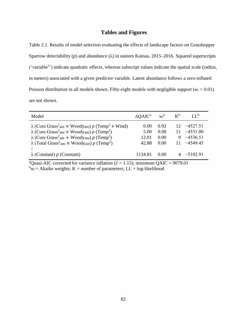
82
Tables and Figures
Table 2.1. Results of model selection evaluating the effects of landscape factors on Grasshopper
Sparrow detectability (p) and abundance (λ) in eastern Kansas, 2015–2016. Squared superscripts
(‘variable2’) indicate quadratic effects, whereas subscript values indicate the spatial scale (radius,
in meters) associated with a given predictor variable. Latent abundance follows a zero-inflated
Poisson distribution in all models shown. Fifty-eight models with negligible support (wi < 0.01)
are not shown.
Model ∆QAICa wib Kb LLb
λ (Core Grass2400 × Woody400) p (Temp2 + Wind) 0.00 0.92 12 −4527.51
λ (Core Grass2400 × Woody400) p (Temp2) 5.00 0.08 11 −4531.00
λ (Core Grass2400 + Woody400) p (Temp2) 12.01 0.00 9 −4536.51
λ (Total Grass2400 × Woody400) p (Temp2) 42.88 0.00 11 −4549.45
⋮
λ (Constant) p (Constant) 1134.81 0.00 4 −5102.91
aQuasi-AIC corrected for variance inflation (�̂� = 1.15); minimum QAIC = 9079.01 bwi = Akaike weights; K = number of parameters; LL = log-likelihood
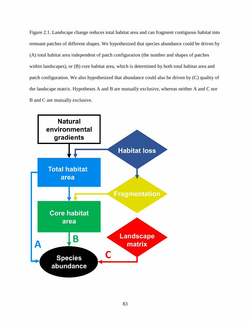
83
Figure 2.1. Landscape change reduces total habitat area and can fragment contiguous habitat into
remnant patches of different shapes. We hypothesized that species abundance could be driven by
(A) total habitat area independent of patch configuration (the number and shapes of patches
within landscapes), or (B) core habitat area, which is determined by both total habitat area and
patch configuration. We also hypothesized that abundance could also be driven by (C) quality of
the landscape matrix. Hypotheses A and B are mutually exclusive, whereas neither A and C nor
B and C are mutually exclusive.
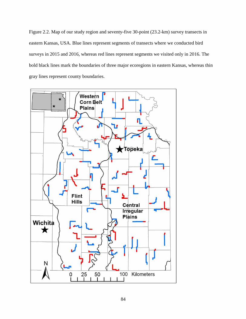
84
Figure 2.2. Map of our study region and seventy-five 30-point (23.2-km) survey transects in
eastern Kansas, USA. Blue lines represent segments of transects where we conducted bird
surveys in 2015 and 2016, whereas red lines represent segments we visited only in 2016. The
bold black lines mark the boundaries of three major ecoregions in eastern Kansas, whereas thin
gray lines represent county boundaries.
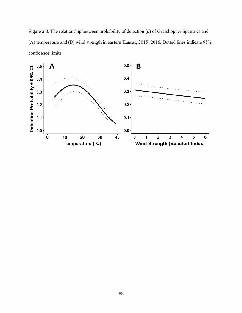
85
Figure 2.3. The relationship between probability of detection (p) of Grasshopper Sparrows and
(A) temperature and (B) wind strength in eastern Kansas, 2015−2016. Dotted lines indicate 95%
confidence limits.
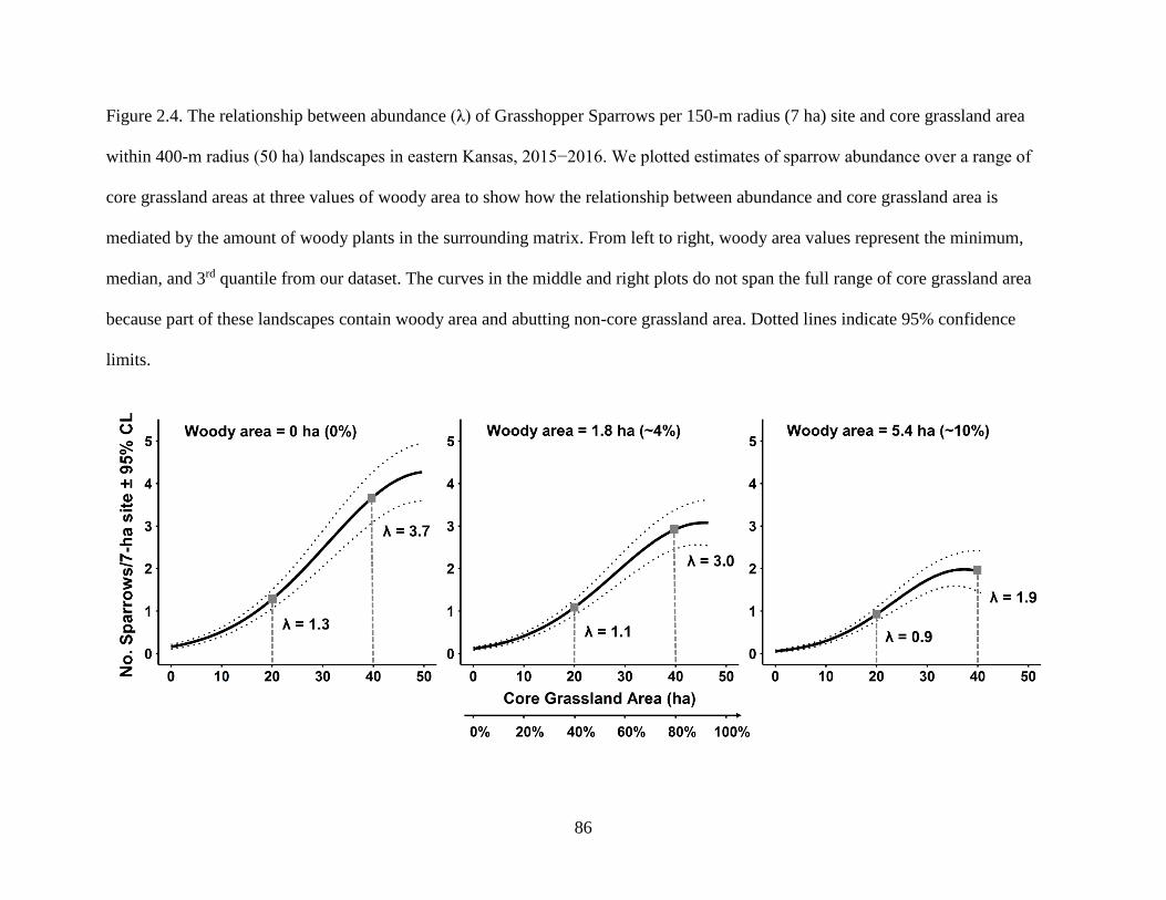
86
Figure 2.4. The relationship between abundance (λ) of Grasshopper Sparrows per 150-m radius (7 ha) site and core grassland area
within 400-m radius (50 ha) landscapes in eastern Kansas, 2015−2016. We plotted estimates of sparrow abundance over a range of
core grassland areas at three values of woody area to show how the relationship between abundance and core grassland area is
mediated by the amount of woody plants in the surrounding matrix. From left to right, woody area values represent the minimum,
median, and 3rd quantile from our dataset. The curves in the middle and right plots do not span the full range of core grassland area
because part of these landscapes contain woody area and abutting non-core grassland area. Dotted lines indicate 95% confidence
limits.
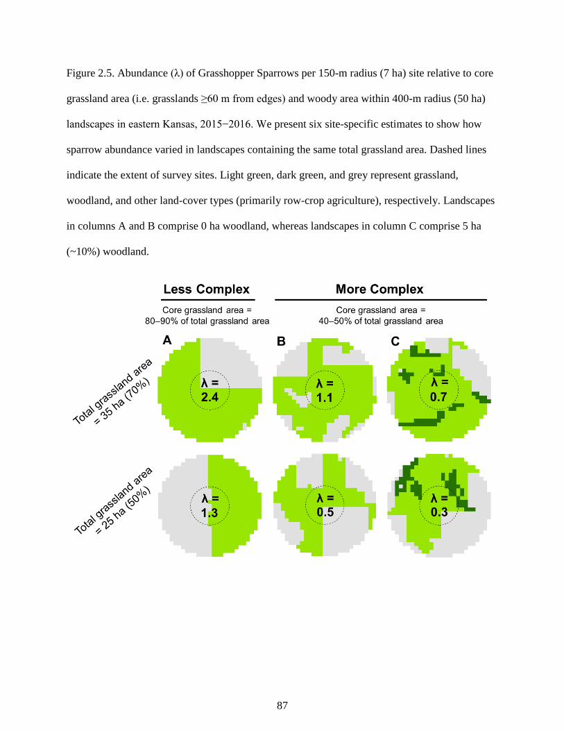
87
Figure 2.5. Abundance (λ) of Grasshopper Sparrows per 150-m radius (7 ha) site relative to core
grassland area (i.e. grasslands ≥60 m from edges) and woody area within 400-m radius (50 ha)
landscapes in eastern Kansas, 2015−2016. We present six site-specific estimates to show how
sparrow abundance varied in landscapes containing the same total grassland area. Dashed lines
indicate the extent of survey sites. Light green, dark green, and grey represent grassland,
woodland, and other land-cover types (primarily row-crop agriculture), respectively. Landscapes
in columns A and B comprise 0 ha woodland, whereas landscapes in column C comprise 5 ha
(~10%) woodland.
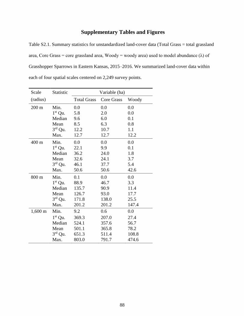
88
Supplementary Tables and Figures
Table S2.1. Summary statistics for unstandardized land-cover data (Total Grass = total grassland
area, Core Grass = core grassland area, Woody = woody area) used to model abundance (λ) of
Grasshopper Sparrows in Eastern Kansas, 2015–2016. We summarized land-cover data within
each of four spatial scales centered on 2,249 survey points.
Scale
(radius)
Statistic Variable (ha)
Total Grass Core Grass Woody
200 m Min. 0.0 0.0 0.0
1st Qu. 5.8 2.0 0.0
Median 9.6 6.0 0.1
Mean 8.5 6.3 0.8
3rd Qu. 12.2 10.7 1.1
Max. 12.7 12.7 12.2
400 m Min. 0.0 0.0 0.0
1st Qu. 22.1 9.9 0.1
Median 36.2 24.0 1.8
Mean 32.6 24.1 3.7
3rd Qu. 46.1 37.7 5.4
Max. 50.6 50.6 42.6
800 m Min. 0.1 0.0 0.0
1st Qu. 88.9 46.7 3.3
Median 135.7 90.9 11.4
Mean 126.7 93.0 17.7
3rd Qu. 171.8 138.0 25.5
Max. 201.2 201.2 147.4
1,600 m Min. 9.2 0.6 0.0
1st Qu. 369.3 207.0 27.4
Median 524.1 357.6 56.7
Mean 501.1 365.8 78.2
3rd Qu. 651.3 511.4 108.8
Max. 803.0 791.7 474.6
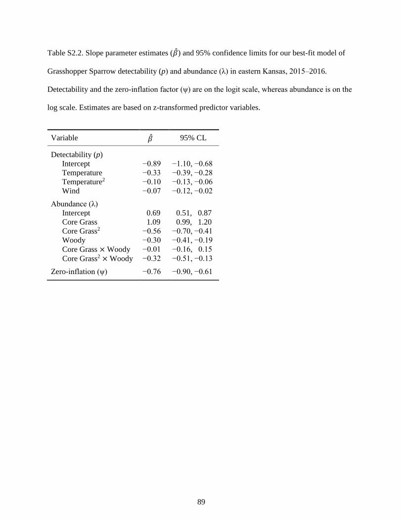
89
Table S2.2. Slope parameter estimates (�̂�) and 95% confidence limits for our best-fit model of
Grasshopper Sparrow detectability (p) and abundance (λ) in eastern Kansas, 2015–2016.
Detectability and the zero-inflation factor (ψ) are on the logit scale, whereas abundance is on the
log scale. Estimates are based on z-transformed predictor variables.
Variable �̂� 95% CL
Detectability (p)
Intercept −0.89 −1.10, −0.68
Temperature −0.33 −0.39, −0.28
Temperature2 −0.10 −0.13, −0.06
Wind −0.07 −0.12, −0.02
Abundance (λ)
Intercept 0.69 0.51, 0.87
Core Grass 1.09 0.99, 1.20
Core Grass2 −0.56 −0.70, −0.41
Woody −0.30 −0.41, −0.19
Core Grass × Woody −0.01 −0.16, 0.15
Core Grass2 × Woody −0.32 −0.51, −0.13
Zero-inflation (ψ) −0.76 −0.90, −0.61
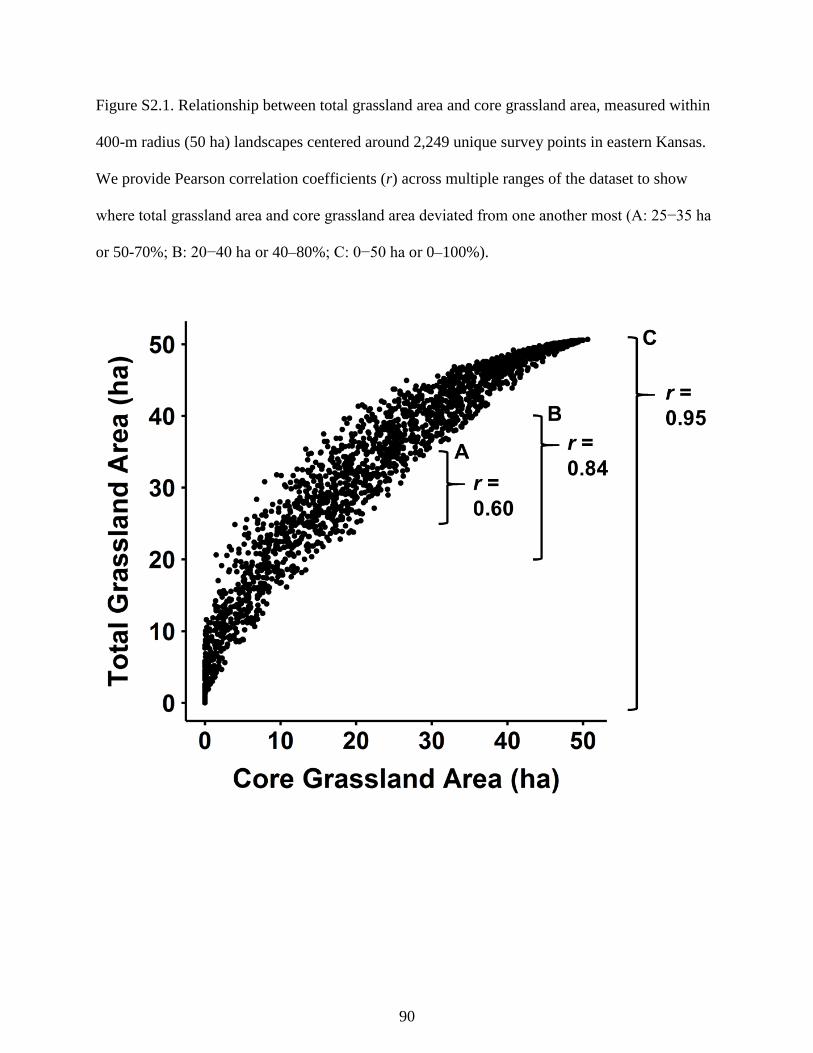
90
Figure S2.1. Relationship between total grassland area and core grassland area, measured within
400-m radius (50 ha) landscapes centered around 2,249 unique survey points in eastern Kansas.
We provide Pearson correlation coefficients (r) across multiple ranges of the dataset to show
where total grassland area and core grassland area deviated from one another most (A: 25−35 ha
or 50-70%; B: 20−40 ha or 40–80%; C: 0−50 ha or 0–100%).