R

If

Da

b

c

h

••••

a

ARRAA

KAACELF

1

1

c2T

b

(

0h

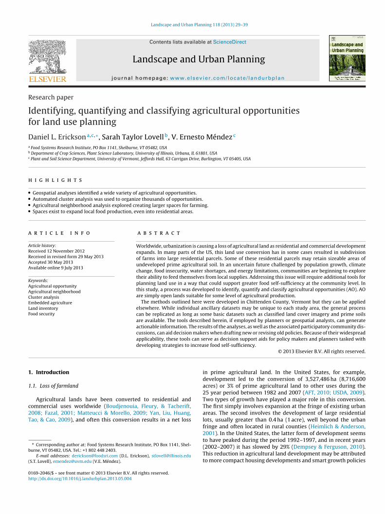
Landscape and Urban Planning 118 (2013) 29– 39

Contents lists available at ScienceDirect

Landscape and Urban Planning

jou rn al hom ep age: www.elsev ier .com/ locate / landurbplan

esearch paper

dentifying, quantifying and classifying agricultural opportunitiesor land use planning

aniel L. Ericksona,c,∗, Sarah Taylor Lovellb, V. Ernesto Méndezc

Food Systems Research Institute, PO Box 1141, Shelburne, VT 05482, USADepartment of Crop Sciences, Plant Science Laboratory, University of Illinois, Urbana, IL 61801, USAPlant and Soil Science Department, University of Vermont, Jeffords Hall, 63 Carrigan Drive, Burlington, VT 05405, USA

i g h l i g h t s

Geospatial analyses identified a wide variety of agricultural opportunities.Automated cluster analysis was used to organize thousands of opportunities.Agricultural neighborhood analysis explored creating larger spaces for farming.Spaces exist to expand local food production, even into residential areas.

r t i c l e i n f o

rticle history:eceived 12 November 2012eceived in revised form 29 May 2013ccepted 30 May 2013vailable online 9 July 2013

eywords:gricultural opportunitygricultural neighborhoodluster analysismbedded agricultureand inventory

a b s t r a c t

Worldwide, urbanization is causing a loss of agricultural land as residential and commercial developmentexpands. In many parts of the US, this land use conversion has in some cases resulted in subdivisionof farms into large residential parcels. Some of these residential parcels may retain sizeable areas ofundeveloped prime agricultural soil. In an uncertain future challenged by population growth, climatechange, food insecurity, water shortages, and energy limitations, communities are beginning to exploretheir ability to feed themselves from local supplies. Addressing this issue will require additional tools forplanning land use in a way that could support greater food self-sufficiency at the community level. Inthis study, a process was developed to identify, quantify and classify agricultural opportunities (AO). AOare simply open lands suitable for some level of agricultural production.

The methods outlined here were developed in Chittenden County, Vermont but they can be appliedelsewhere. While individual ancillary datasets may be unique to each study area, the general process

ood security can be replicated as long as some basic datasets such as classified land cover imagery and prime soilsare available. The tools described herein, if employed by planners or geospatial analysts, can generateactionable information. The results of the analyses, as well as the associated participatory community dis-cussions, can aid decision makers when drafting new or revising old policies. Because of their widespreadapplicability, these tools can serve as decision support aids for policy makers and planners tasked with

ncrea

developing strategies to i

. Introduction

.1. Loss of farmland

Agricultural lands have been converted to residential and

ommercial uses worldwide (Boudjenouia, Fleury, & Tacherift,008; Fazal, 2001; Matteucci & Morello, 2009; Yan, Liu, Huang,ao, & Cao, 2009), and often this conversion results in a net loss

∗ Corresponding author at: Food Systems Research Institute, PO Box 1141, Shel-urne, VT 05482, USA. Tel.: +1 802 448 2403.

E-mail addresses: derickson@foodsri.com (D.L. Erickson), stlovell@illinois.eduS.T. Lovell), emendez@uvm.edu (V.E. Méndez).

169-2046/$ – see front matter © 2013 Elsevier B.V. All rights reserved.ttp://dx.doi.org/10.1016/j.landurbplan.2013.05.004

se food self-sufficiency.© 2013 Elsevier B.V. All rights reserved.

in prime agricultural land. In the United States, for example,development led to the conversion of 3,527,486 ha (8,716,600acres) or 3% of prime agricultural land to other uses during the25 year period between 1982 and 2007 (AFT, 2010; USDA, 2009).Two types of growth have played a major role in this conversion.The first simply involves expansion at the fringe of existing urbanareas. The second involves the development of large residentiallots, usually greater than 0.4 ha (1 acre), well beyond the urbanfringe and often located in rural counties (Heimlich & Anderson,2001). In the United States, the latter form of development seems

to have peaked during the period 1992–1997, and in recent years(2002–2007) it has slowed by 29% (Dempsey & Ferguson, 2010).This reduction in agricultural land development may be attributedto more compact housing developments and smart growth policies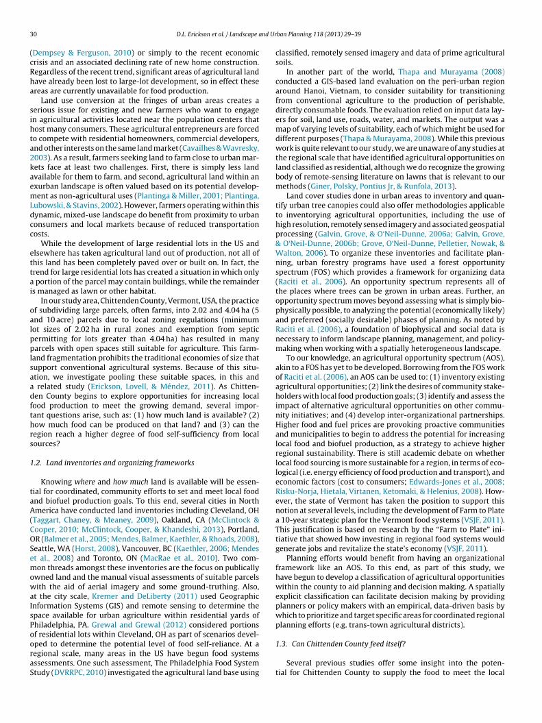

3 nd Ur

(cRha

sihta2kaemLdcc

ettai

oalpplsaadfthrs

1

taA(COSemowaIsPooraS

0 D.L. Erickson et al. / Landscape a

Dempsey & Ferguson, 2010) or simply to the recent economicrisis and an associated declining rate of new home construction.egardless of the recent trend, significant areas of agricultural landave already been lost to large-lot development, so in effect thesereas are currently unavailable for food production.

Land use conversion at the fringes of urban areas creates aerious issue for existing and new farmers who want to engagen agricultural activities located near the population centers thatost many consumers. These agricultural entrepreneurs are forcedo compete with residential homeowners, commercial developers,nd other interests on the same land market (Cavailhes & Wavresky,003). As a result, farmers seeking land to farm close to urban mar-ets face at least two challenges. First, there is simply less landvailable for them to farm, and second, agricultural land within anxurban landscape is often valued based on its potential develop-ent as non-agricultural uses (Plantinga & Miller, 2001; Plantinga,

ubowski, & Stavins, 2002). However, farmers operating within thisynamic, mixed-use landscape do benefit from proximity to urbanonsumers and local markets because of reduced transportationosts.

While the development of large residential lots in the US andlsewhere has taken agricultural land out of production, not all ofhis land has been completely paved over or built on. In fact, therend for large residential lots has created a situation in which only

portion of the parcel may contain buildings, while the remainders managed as lawn or other habitat.

In our study area, Chittenden County, Vermont, USA, the practicef subdividing large parcels, often farms, into 2.02 and 4.04 ha (5nd 10 acre) parcels due to local zoning regulations (minimumot sizes of 2.02 ha in rural zones and exemption from septicermitting for lots greater than 4.04 ha) has resulted in manyarcels with open spaces still suitable for agriculture. This farm-

and fragmentation prohibits the traditional economies of size thatupport conventional agricultural systems. Because of this situ-tion, we investigate pooling these suitable spaces, in this and

related study (Erickson, Lovell, & Méndez, 2011). As Chitten-en County begins to explore opportunities for increasing localood production to meet the growing demand, several impor-ant questions arise, such as: (1) how much land is available? (2)ow much food can be produced on that land? and (3) can theegion reach a higher degree of food self-sufficiency from localources?

.2. Land inventories and organizing frameworks

Knowing where and how much land is available will be essen-ial for coordinated, community efforts to set and meet local foodnd biofuel production goals. To this end, several cities in Northmerica have conducted land inventories including Cleveland, OH

Taggart, Chaney, & Meaney, 2009), Oakland, CA (McClintock &ooper, 2010; McClintock, Cooper, & Khandeshi, 2013), Portland,R (Balmer et al., 2005; Mendes, Balmer, Kaethler, & Rhoads, 2008),eattle, WA (Horst, 2008), Vancouver, BC (Kaethler, 2006; Mendest al., 2008) and Toronto, ON (MacRae et al., 2010). Two com-on threads amongst these inventories are the focus on publically

wned land and the manual visual assessments of suitable parcelsith the aid of aerial imagery and some ground-truthing. Also,

t the city scale, Kremer and DeLiberty (2011) used Geographicnformation Systems (GIS) and remote sensing to determine thepace available for urban agriculture within residential yards ofhiladelphia, PA. Grewal and Grewal (2012) considered portionsf residential lots within Cleveland, OH as part of scenarios devel-

ped to determine the potential level of food self-reliance. At aegional scale, many areas in the US have begun food systemsssessments. One such assessment, The Philadelphia Food Systemtudy (DVRRPC, 2010) investigated the agricultural land base using

ban Planning 118 (2013) 29– 39

classified, remotely sensed imagery and data of prime agriculturalsoils.

In another part of the world, Thapa and Murayama (2008)conducted a GIS-based land evaluation on the peri-urban regionaround Hanoi, Vietnam, to consider suitability for transitioningfrom conventional agriculture to the production of perishable,directly consumable foods. The evaluation relied on input data lay-ers for soil, land use, roads, water, and markets. The output was amap of varying levels of suitability, each of which might be used fordifferent purposes (Thapa & Murayama, 2008). While this previouswork is quite relevant to our study, we are unaware of any studies atthe regional scale that have identified agricultural opportunities onland classified as residential, although we do recognize the growingbody of remote-sensing literature on lawns that is relevant to ourmethods (Giner, Polsky, Pontius Jr, & Runfola, 2013).

Land cover studies done in urban areas to inventory and quan-tify urban tree canopies could also offer methodologies applicableto inventorying agricultural opportunities, including the use ofhigh resolution, remotely sensed imagery and associated geospatialprocessing (Galvin, Grove, & O‘Neil-Dunne, 2006a; Galvin, Grove,& O‘Neil-Dunne, 2006b; Grove, O‘Neil-Dunne, Pelletier, Nowak, &Walton, 2006). To organize these inventories and facilitate plan-ning, urban forestry programs have used a forest opportunityspectrum (FOS) which provides a framework for organizing data(Raciti et al., 2006). An opportunity spectrum represents all ofthe places where trees can be grown in urban areas. Further, anopportunity spectrum moves beyond assessing what is simply bio-physically possible, to analyzing the potential (economically likely)and preferred (socially desirable) phases of planning. As noted byRaciti et al. (2006), a foundation of biophysical and social data isnecessary to inform landscape planning, management, and policy-making when working with a spatially heterogeneous landscape.

To our knowledge, an agricultural opportunity spectrum (AOS),akin to a FOS has yet to be developed. Borrowing from the FOS workof Raciti et al. (2006), an AOS can be used to: (1) inventory existingagricultural opportunities; (2) link the desires of community stake-holders with local food production goals; (3) identify and assess theimpact of alternative agricultural opportunities on other commu-nity initiatives; and (4) develop inter-organizational partnerships.Higher food and fuel prices are provoking proactive communitiesand municipalities to begin to address the potential for increasinglocal food and biofuel production, as a strategy to achieve higherregional sustainability. There is still academic debate on whetherlocal food sourcing is more sustainable for a region, in terms of eco-logical (i.e. energy efficiency of food production and transport), andeconomic factors (cost to consumers; Edwards-Jones et al., 2008;Risku-Norja, Hietala, Virtanen, Ketomaki, & Helenius, 2008). How-ever, the state of Vermont has taken the position to support thisnotion at several levels, including the development of Farm to Platea 10-year strategic plan for the Vermont food systems (VSJF, 2011).This justification is based on research by the “Farm to Plate” ini-tiative that showed how investing in regional food systems wouldgenerate jobs and revitalize the state’s economy (VSJF, 2011).

Planning efforts would benefit from having an organizationalframework like an AOS. To this end, as part of this study, wehave begun to develop a classification of agricultural opportunitieswithin the county to aid planning and decision making. A spatiallyexplicit classification can facilitate decision making by providingplanners or policy makers with an empirical, data-driven basis bywhich to prioritize and target specific areas for coordinated regionalplanning efforts (e.g. trans-town agricultural districts).

1.3. Can Chittenden County feed itself?

Several previous studies offer some insight into the poten-tial for Chittenden County to supply the food to meet the local

D.L. Erickson et al. / Landscape and Urban Planning 118 (2013) 29– 39 31

cation

nlpeACltwbd4(tbp

1

cbspsotswommapcTttcc

Fig. 1. Regional lo

eeds. One study found that Toronto, Canada, a city with a sim-ar climate to Burlington’s, would need 2317 ha of land (if allroduction is organic) to produce 10% of the annual fresh veg-table needs for its 2.5 million residents (MacRae et al., 2010).

study conducted locally by McKellips (2009) estimated thathittenden and its five neighboring counties needed additional

and to supply the demand for local foods: 572 ha of addi-ional vegetable production, 2064 additional hectares of hardheat, and 11,509 ha of land dedicated to fodder crops for local

eef and pork production. The study also noted that Chitten-en and its surrounding counties have 78,934 dairy cows and49 ha of apple orchards beyond what is needed for local demandMcKellips, 2009). These studies suggest that there is some poten-ial for Chittenden County to become more food self-sufficient,ut they offer little in terms of planning goals to make that hap-en.

.4. Purpose of study

In an uncertain future challenged by climate change, food inse-urity, water shortages, and energy limitations, communities areeginning to explore their ability to feed themselves from localupplies. Addressing this issue will require additional tools forlanning land use in a way that could support greater food self-ufficiency at the community level. To this end, the primary goalf this research was to develop a process by which to iden-ify, quantify and organize (classify) agricultural opportunity (AO)paces in order to facilitate regional planning efforts concernedith increasing local food self-sufficiency. An AO is simply any

pen land suitable for some level of agricultural production. Theethods outlined here were developed in Chittenden County, Ver-ont, but they can be applied elsewhere. While the individual

ncillary datasets may be unique to each study area, the generalrocess can be replicated as long as some basic datasets, such aslassified land cover imagery and agricultural soils are available.he tools described herein, if employed by planners or geospa-

ial analysts, can generate actionable information. The results ofhe analyses, as well as the associated community discussions,an aid decision makers when drafting new or revising old poli-ies.

of the study area.

2. Methods

2.1. Study area

Our study was conducted in Chittenden County, located in theChamplain Valley of Vermont. The county extends east from theshores of Lake Champlain to the foothills and ridgelines of theGreen Mountains, and is home to the City of Burlington, Vermont’smost densely populated and built-up urban area (Fig. 1). The totalestimated county population is 156,545 (USCB, 2011), and the pop-ulation density is 112 per km2 (291/mi2). The median householdincome in 2011 was $62,260, with 10.9% of county residents livingbelow the poverty line. The 2010–2011 2-year averages in Ver-mont and the US were $54,777 and $50,443 respectively (USCB,2013). Within the Burlington School District, 46% of enrolled stu-dents qualified for free or reduced price meals, while 26% qualifywithin the county as a whole (VTDoE, 2012). There are 66,345 hous-ing units with a median value of owner occupied units of $263,200(USCB, 2011). The landcover of the county consists of mostly nat-ural, pervious surfaces. Despite the presence of Burlington and itsimmediate neighboring surburban towns, only about 10.6% of theland area of the county is truly developed (i.e. occupied by build-ings and other impervious surfaces). The surrounding towns arestill largely rural in character with a heterogeneous landscape oftown centers, suburban housing developments, farms and forests.The majority of the undeveloped area in the County is forested(61.5%), with the balance a mix of open land–lawns and agriculturalfields (22.5%). The remainder consists of water, wetlands and barrensites. In 2008, Chittenden County had 39,573 land parcels (total-ing 54,083 ha) with residential use, as classified by the ChittendenCounty Regional Planning Commision (CCRPC). Their classificationwas based on the American Planning Association’s Land-Based Clas-sification Standards (APA, 2010).

2.2. Geospatial database development

A geographic information system (GIS) was assembled withfreely available spatial data layers acquired from the Vermont Cen-ter for Geographic Information (VCGI), the University of VermontSpatial Analysis Lab (UVM-SAL), the Chittenden County Regional

32 D.L. Erickson et al. / Landscape and Urban Planning 118 (2013) 29– 39

origin

PsCl

2

oC80mtga

cslwittdcti3

swCrdrvahpataciueiws

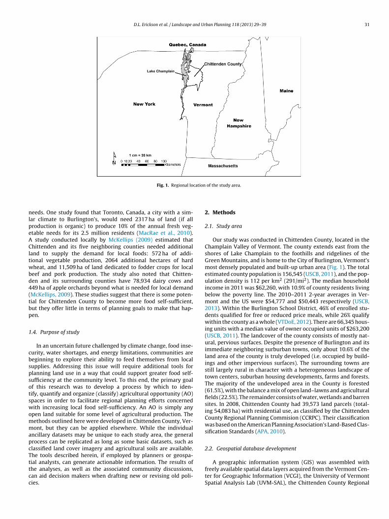
Fig. 2. Comparison of (a) NAIP orthoimage, (b)

lanning Comission (CCRPC), the National Oceanic and Atmo-pheric Administration’s Coastal Change Analysis Program (NOAA-CAP) and ArcGIS Online. These data sets were assembled, ana-

yzed, and processed in ESRI® ArcMapTM 9.3.1 and later 10.0.

.2.1. Geospatial analysisA 2006 NOAA C-CAP land cover image, with a 30 m2 res-

lution was downloaded from the NOAA C-CAP web site. The-CAP data product is developed to have an overall accuracy of5% (NOAA, 2011). The image was visually cross checked against.16 m2 orthoimagery from 2004, but no formal accuracy assess-ent was conducted. We believe the accuracy and resolution of

he imagery used is suitable for this ‘first pass’ analysis. However,round truthing and/or the use of higher reolution imagery is warr-nted before enacting new land use policies.

To facilitate subsequent processing, the land cover image waslipped to the study area and reclassified from 19 classes toix: (1) built; (2) open-agriculture-lawns; (3) forested; (4) wet-ands; (5) water; and (6) barren/bare earth. The image cell size

as converted from 30 to 10 m2. This was done to improve themage with respect to the addition of features not captured athe 30 m2 resolution. This change in storage resolution was doneo facilitate updating the source image with ancillary vector GISatalayers. However, to be clear, this change in cell size did nothange the 30 m2 resolution of the land cover data. Thus, withhe exception of some of the additional data layers added to themage, as described below, the image resolution in effect remained0 m2.

The following vector data layers were incorporated into theource image using standard raster overlay procedures: surfaceater, roads, driveways and buildings. Thus, any pixel in the C-AP image that corresponded with a road or driveway pixel waseclassified as built. The cell size of the raster versions of the vectorata varied: driveways were 10 m2, local roads 20 m2 and majoroads 30 m2. Buildings, originally represented as points, were con-erted to a 30 m2 raster. This cell size was chosen because it wasssumed that for small buildings such as residences, even if theyad a smaller footprint, their structure and surrounding lawn orarking area would influence an area of about 30 m2. It was alsossumed that larger buildings were correctly classified as built inhe source image and would thus be larger than one 30 m2 cell. Wecknowledge that these assumptions and the use of the 30 m2 landover imagery may lead to the unintended consequence of remov-ng possible arable land from consideration. Thus, if available, these of land cover data generated from higher resolution imagery is

ncouraged. Fig. 2 illustrates the improvement of the source C-CAPmage. A 2008 National Aerial Imagery Program (NAIP) orthoimage

ith a 1 m2 resolution is also included as a reference for compari-on purposes. Driveways and buildings are now clearly visible in

al C-CAP image and (c) improved C-CAP image.

the center of the improved image (Fig. 2C), and roads are nowconnected and no longer segmented.

The improved land cover image was eventually reduced toa binary image of possible agricultural land. The built, forested,wetlands, water and barren/bare earth were combined into oneclass and coded zero (0) and the open-agriculture-lawns was codedas one (1). While we chose not to include forested land in ouranalysis, users of this approach in other locales may opt to includethis land cover type because of its potential for agroforestry and thegrowing of shade tolerant crops. A percent slope raster was gener-ated from a 10 m2 hydrologically correct digital elevation modelacquired from VCGI. The resulting raster was reclassified into thefollowing 3 classes, based on the USDA slope class definitions(http://soils.usda.gov/technical/manual/contents/chapter3.html):(1) nearly level (0–3%); (2) gently to strongly sloping (3–16%); and(3) steep (>16%). Polygons of prime agricultural soil (defined hereand throughout the rest of the paper as USDA prime soils and thosesoils of statewide importance for agriculture) were converted toa raster. The binary image of possible agricultural land, the slopeand prime agricultural soils raster layers were all merged usingstandard raster overlay procedures. The resulting agriculturalopportunity raster had six classes: (1) open-nearly level, (2)open-moderate slope, (3) open-steep slope, (4) open-nearly level– with prime soil, (5) open-moderate slope – with prime soil and(6) open-steep slope – with prime soil. We acknowledge thatsuch classifications of land may lead to rigidity in using the data.Further, such a simplified classification, meant for a ‘first pass’analysis should not dictate how a farmer should use a given pieceof land.

A polygon data set of land parcels acquired from CCRPC was usedto tabulate the agricultural opportunity classes within each parcel.Each parcel had been coded by the CCRPC using the American Plan-ning Association’s Land Based Classification System (LBCS) (APA,2010). The APA website defines these dimensions as follows:

• “Site” refers to the overall physical development character of theland. In general physical terms, it describes what is on the land.

• “Structure” refers to the type of structure or building present onthe land.

• “Activity” is concerned with the actual use of land based on itsobservable characteristics.

• “Function” refers to the economic function or type of establish-ment that is using the land.

Two Euclidean distance rasters were also generated. The first

was distance from center of Burlington, specifically City Hall. Thesecond was distance from the center of other towns located withinthe county. These distance rasters were generated for inclusion inone of the cluster analyses described below.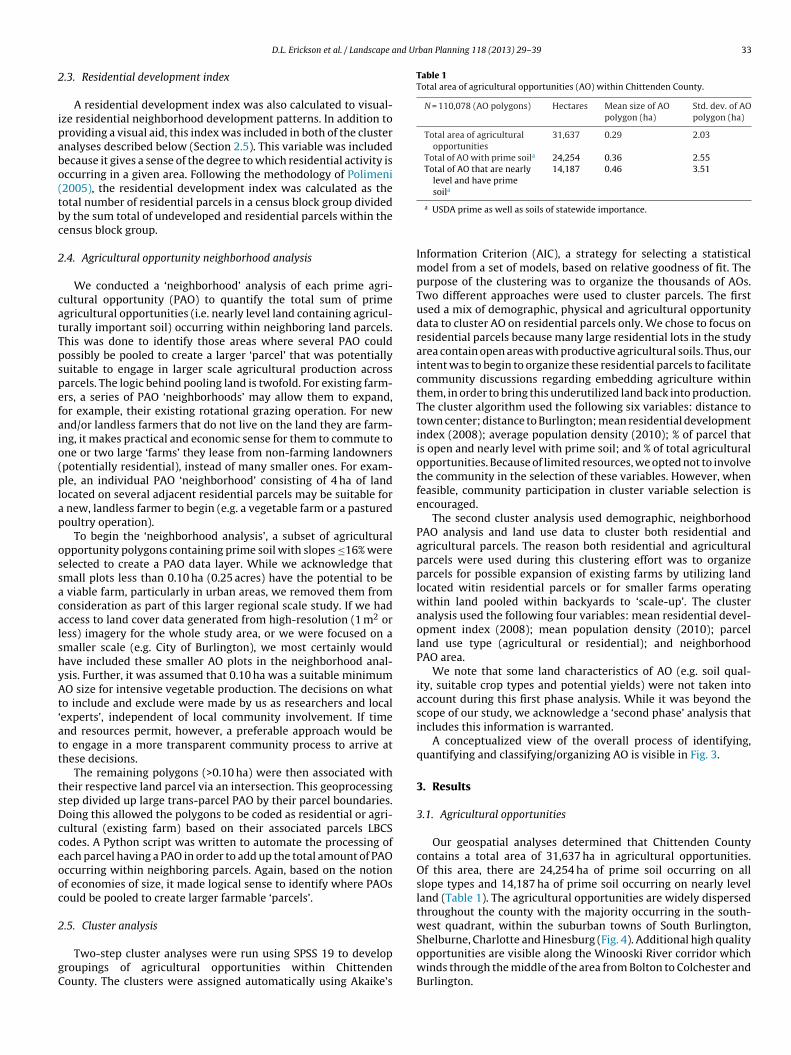

nd Urban Planning 118 (2013) 29– 39 33

2

ipabo(tbc

2

catTpspefaio(plap

ossacalshyAt‘att

tsDcceooc

2

gC

Table 1Total area of agricultural opportunities (AO) within Chittenden County.

N = 110,078 (AO polygons) Hectares Mean size of AOpolygon (ha)

Std. dev. of AOpolygon (ha)

Total area of agriculturalopportunities

31,637 0.29 2.03

Total of AO with prime soila 24,254 0.36 2.55Total of AO that are nearly

level and have primesoila

14,187 0.46 3.51

D.L. Erickson et al. / Landscape a

.3. Residential development index

A residential development index was also calculated to visual-ze residential neighborhood development patterns. In addition toroviding a visual aid, this index was included in both of the clusternalyses described below (Section 2.5). This variable was includedecause it gives a sense of the degree to which residential activity isccurring in a given area. Following the methodology of Polimeni2005), the residential development index was calculated as theotal number of residential parcels in a census block group dividedy the sum total of undeveloped and residential parcels within theensus block group.

.4. Agricultural opportunity neighborhood analysis

We conducted a ‘neighborhood’ analysis of each prime agri-ultural opportunity (PAO) to quantify the total sum of primegricultural opportunities (i.e. nearly level land containing agricul-urally important soil) occurring within neighboring land parcels.his was done to identify those areas where several PAO couldossibly be pooled to create a larger ‘parcel’ that was potentiallyuitable to engage in larger scale agricultural production acrossarcels. The logic behind pooling land is twofold. For existing farm-rs, a series of PAO ‘neighborhoods’ may allow them to expand,or example, their existing rotational grazing operation. For newnd/or landless farmers that do not live on the land they are farm-ng, it makes practical and economic sense for them to commute tone or two large ‘farms’ they lease from non-farming landownerspotentially residential), instead of many smaller ones. For exam-le, an individual PAO ‘neighborhood’ consisting of 4 ha of land

ocated on several adjacent residential parcels may be suitable for new, landless farmer to begin (e.g. a vegetable farm or a pasturedoultry operation).

To begin the ‘neighborhood analysis’, a subset of agriculturalpportunity polygons containing prime soil with slopes ≤16% wereelected to create a PAO data layer. While we acknowledge thatmall plots less than 0.10 ha (0.25 acres) have the potential to be

viable farm, particularly in urban areas, we removed them fromonsideration as part of this larger regional scale study. If we hadccess to land cover data generated from high-resolution (1 m2 oress) imagery for the whole study area, or we were focused on amaller scale (e.g. City of Burlington), we most certainly wouldave included these smaller AO plots in the neighborhood anal-sis. Further, it was assumed that 0.10 ha was a suitable minimumO size for intensive vegetable production. The decisions on what

o include and exclude were made by us as researchers and localexperts’, independent of local community involvement. If timend resources permit, however, a preferable approach would beo engage in a more transparent community process to arrive athese decisions.

The remaining polygons (>0.10 ha) were then associated withheir respective land parcel via an intersection. This geoprocessingtep divided up large trans-parcel PAO by their parcel boundaries.oing this allowed the polygons to be coded as residential or agri-ultural (existing farm) based on their associated parcels LBCSodes. A Python script was written to automate the processing ofach parcel having a PAO in order to add up the total amount of PAOccurring within neighboring parcels. Again, based on the notionf economies of size, it made logical sense to identify where PAOsould be pooled to create larger farmable ‘parcels’.

.5. Cluster analysis

Two-step cluster analyses were run using SPSS 19 to developroupings of agricultural opportunities within Chittendenounty. The clusters were assigned automatically using Akaike’s

a USDA prime as well as soils of statewide importance.

Information Criterion (AIC), a strategy for selecting a statisticalmodel from a set of models, based on relative goodness of fit. Thepurpose of the clustering was to organize the thousands of AOs.Two different approaches were used to cluster parcels. The firstused a mix of demographic, physical and agricultural opportunitydata to cluster AO on residential parcels only. We chose to focus onresidential parcels because many large residential lots in the studyarea contain open areas with productive agricultural soils. Thus, ourintent was to begin to organize these residential parcels to facilitatecommunity discussions regarding embedding agriculture withinthem, in order to bring this underutilized land back into production.The cluster algorithm used the following six variables: distance totown center; distance to Burlington; mean residential developmentindex (2008); average population density (2010); % of parcel thatis open and nearly level with prime soil; and % of total agriculturalopportunities. Because of limited resources, we opted not to involvethe community in the selection of these variables. However, whenfeasible, community participation in cluster variable selection isencouraged.

The second cluster analysis used demographic, neighborhoodPAO analysis and land use data to cluster both residential andagricultural parcels. The reason both residential and agriculturalparcels were used during this clustering effort was to organizeparcels for possible expansion of existing farms by utilizing landlocated witin residential parcels or for smaller farms operatingwithin land pooled within backyards to ‘scale-up’. The clusteranalysis used the following four variables: mean residential devel-opment index (2008); mean population density (2010); parcelland use type (agricultural or residential); and neighborhoodPAO area.

We note that some land characteristics of AO (e.g. soil qual-ity, suitable crop types and potential yields) were not taken intoaccount during this first phase analysis. While it was beyond thescope of our study, we acknowledge a ‘second phase’ analysis thatincludes this information is warranted.

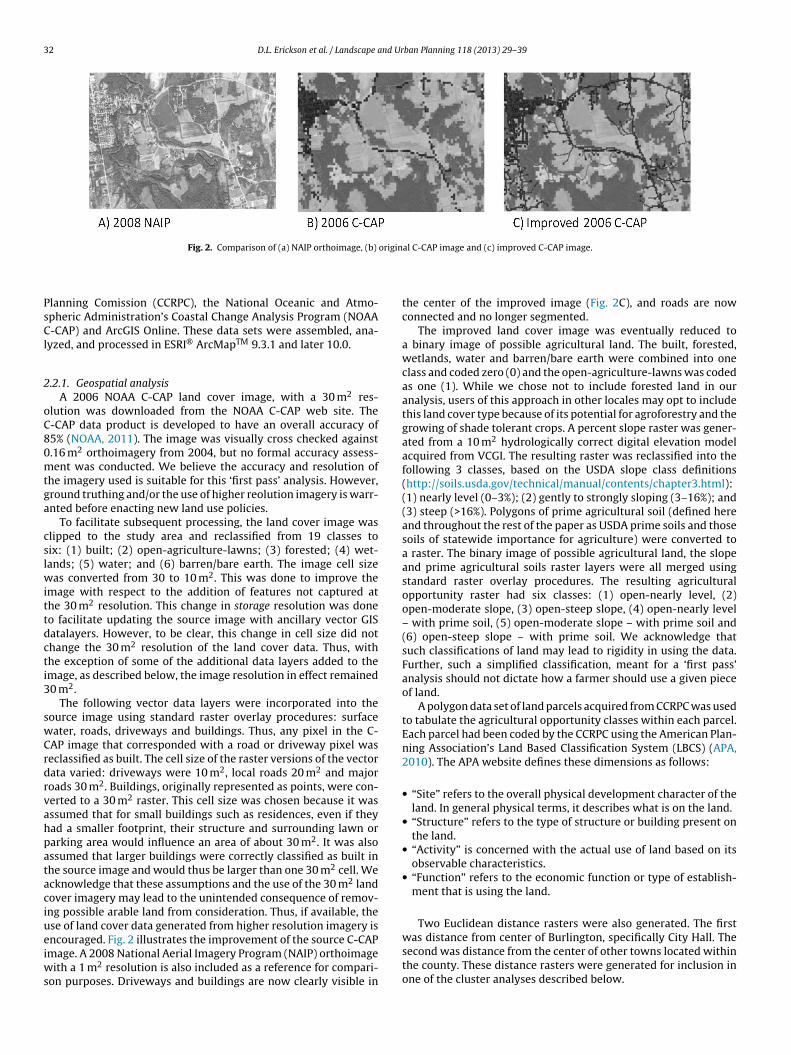
A conceptualized view of the overall process of identifying,quantifying and classifying/organizing AO is visible in Fig. 3.

3. Results

3.1. Agricultural opportunities

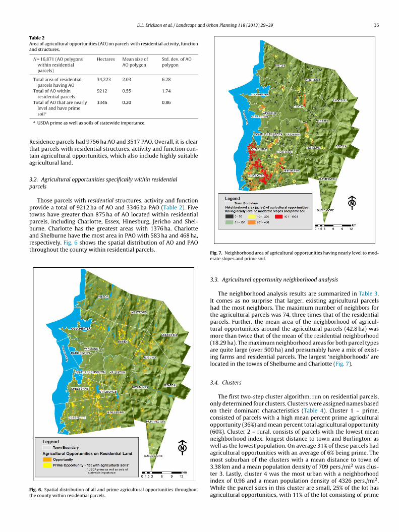
Our geospatial analyses determined that Chittenden Countycontains a total area of 31,637 ha in agricultural opportunities.Of this area, there are 24,254 ha of prime soil occurring on allslope types and 14,187 ha of prime soil occurring on nearly levelland (Table 1). The agricultural opportunities are widely dispersedthroughout the county with the majority occurring in the south-west quadrant, within the suburban towns of South Burlington,

Shelburne, Charlotte and Hinesburg (Fig. 4). Additional high qualityopportunities are visible along the Winooski River corridor whichwinds through the middle of the area from Bolton to Colchester andBurlington.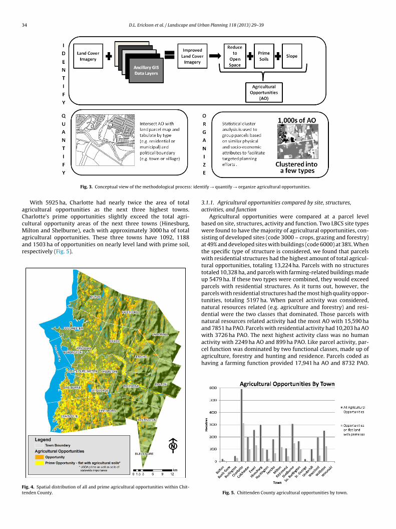

34 D.L. Erickson et al. / Landscape and Urban Planning 118 (2013) 29– 39

: iden

aCcMaar

Ft

Fig. 3. Conceptual view of the methodological process

With 5925 ha, Charlotte had nearly twice the area of totalgricultural opportunities as the next three highest towns.harlotte’s prime opportunities slightly exceed the total agri-ultural opportunity areas of the next three towns (Hinesburg,

ilton and Shelburne), each with approximately 3000 ha of total

gricultural opportunities. These three towns have 1092, 1188nd 1503 ha of opportunities on nearly level land with prime soil,espectively (Fig. 5).

ig. 4. Spatial distribution of all and prime agricultural opportunities within Chit-enden County.

tify → quantify → organize agricultural opportunities.

3.1.1. Agricultural opportunities compared by site, structures,activities, and function

Agricultural opportunities were compared at a parcel levelbased on site, structures, activity and function. Two LBCS site typeswere found to have the majority of agricultural opportunities, con-sisting of developed sites (code 3000 – crops, grazing and forestry)at 49% and developed sites with buildings (code 6000) at 38%. Whenthe specific type of structure is considered, we found that parcelswith residential structures had the highest amount of total agricul-tural opportunities, totaling 13,224 ha. Parcels with no structurestotaled 10,328 ha, and parcels with farming-related buildings madeup 5479 ha. If these two types were combined, they would exceedparcels with residential structures. As it turns out, however, theparcels with residential structures had the most high quality oppor-tunities, totaling 5197 ha. When parcel activity was considered,natural resources related (e.g. agriculture and forestry) and resi-dential were the two classes that dominated. Those parcels withnatural resources related activity had the most AO with 15,590 haand 7851 ha PAO. Parcels with residential activity had 10,203 ha AOwith 3726 ha PAO. The next highest activity class was no humanactivity with 2249 ha AO and 899 ha PAO. Like parcel activity, par-

cel function was dominated by two functional classes, made up ofagriculture, forestry and hunting and residence. Parcels coded ashaving a farming function provided 17,941 ha AO and 8732 PAO.

Fig. 5. Chittenden County agricultural opportunities by town.

D.L. Erickson et al. / Landscape and Urban Planning 118 (2013) 29– 39 35

Table 2Area of agricultural opportunities (AO) on parcels with residential activity, functionand structures.

N = 16,871 (AO polygonswithin residentialparcels)

Hectares Mean size ofAO polygon

Std. dev. of AOpolygon

Total area of residentialparcels having AO

34,223 2.03 6.28

Total of AO withinresidential parcels

9212 0.55 1.74

Total of AO that are nearlylevel and have prime

3346 0.20 0.86

Rtta

3p

ptpbart

Ft

soila

a USDA prime as well as soils of statewide importance.

esidence parcels had 9756 ha AO and 3517 PAO. Overall, it is clearhat parcels with residential structures, activity and function con-ain agricultural opportunities, which also include highly suitablegricultural land.

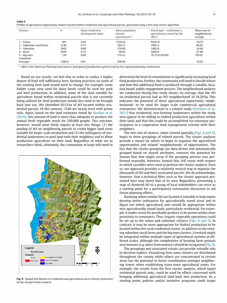
.2. Agricultural opportunities specifically within residentialarcels

Those parcels with residential structures, activity and functionrovide a total of 9212 ha of AO and 3346 ha PAO (Table 2). Fiveowns have greater than 875 ha of AO located within residentialarcels, including Charlotte, Essex, Hinesburg, Jericho and Shel-urne. Charlotte has the greatest areas with 1376 ha. Charlotte

nd Shelburne have the most area in PAO with 583 ha and 468 ha,espectively. Fig. 6 shows the spatial distribution of AO and PAOhroughout the county within residential parcels.

ig. 6. Spatial distribution of all and prime agricultural opportunities throughouthe county within residential parcels.

Fig. 7. Neighborhood area of agricultural opportunities having nearly level to mod-erate slopes and prime soil.

3.3. Agricultural opportunity neighborhood analysis

The neighborhood analysis results are summarized in Table 3.It comes as no surprise that larger, existing agricultural parcelshad the most neighbors. The maximum number of neighbors forthe agricultural parcels was 74, three times that of the residentialparcels. Further, the mean area of the neighborhood of agricul-tural opportunities around the agricultural parcels (42.8 ha) wasmore than twice that of the mean of the residential neighborhood(18.29 ha). The maximum neighborhood areas for both parcel typesare quite large (over 500 ha) and presumably have a mix of exist-ing farms and residential parcels. The largest ‘neighborhoods’ arelocated in the towns of Shelburne and Charlotte (Fig. 7).

3.4. Clusters

The first two-step cluster algorithm, run on residential parcels,only determined four clusters. Clusters were assigned names basedon their dominant characteristics (Table 4). Cluster 1 – prime,consisted of parcels with a high mean percent prime agriculturalopportunity (36%) and mean percent total agricultural opportunity(60%). Cluster 2 – rural, consists of parcels with the lowest meanneighborhood index, longest distance to town and Burlington, aswell as the lowest population. On average 31% of these parcels hadagricultural opportunities with an average of 6% being prime. Themost suburban of the clusters with a mean distance to town of3.38 km and a mean population density of 709 pers./mi2 was clus-ter 3. Lastly, cluster 4 was the most urban with a neighborhood

index of 0.96 and a mean population density of 4326 pers./mi2.While the parcel sizes in this cluster are small, 25% of the lot hasagricultural opportunities, with 11% of the lot consisting of prime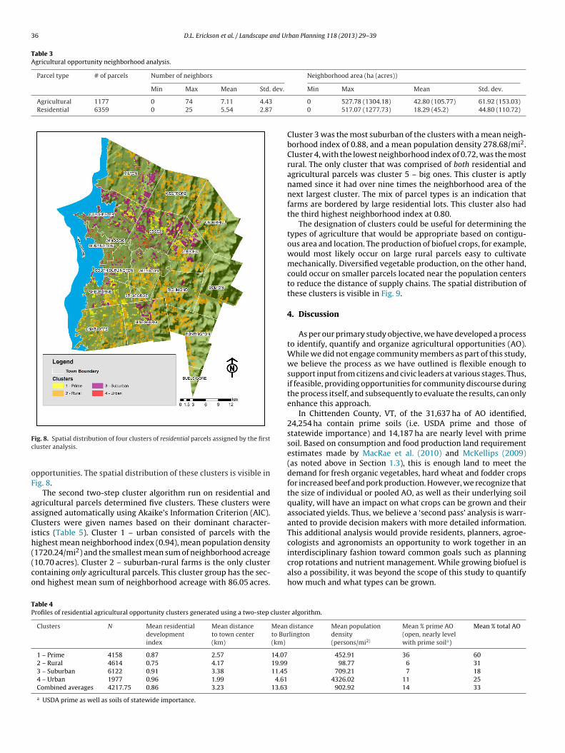

36 D.L. Erickson et al. / Landscape and Urban Planning 118 (2013) 29– 39

Table 3Agricultural opportunity neighborhood analysis.

Parcel type # of parcels Number of neighbors Neighborhood area (ha (acres))

Min Max Mean Std. dev. Min Max Mean Std. dev.

Agricultural 1177 0 74 7.11 4.43

Residential 6359 0 25 5.54 2.87

Fc

oF

aaCih((co

TP

ig. 8. Spatial distribution of four clusters of residential parcels assigned by the firstluster analysis.

pportunities. The spatial distribution of these clusters is visible inig. 8.

The second two-step cluster algorithm run on residential andgricultural parcels determined five clusters. These clusters weressigned automatically using Akaike’s Information Criterion (AIC).lusters were given names based on their dominant character-

stics (Table 5). Cluster 1 – urban consisted of parcels with theighest mean neighborhood index (0.94), mean population density

2

1720.24/mi ) and the smallest mean sum of neighborhood acreage10.70 acres). Cluster 2 – suburban-rural farms is the only clusterontaining only agricultural parcels. This cluster group has the sec-nd highest mean sum of neighborhood acreage with 86.05 acres.

able 4rofiles of residential agricultural opportunity clusters generated using a two-step cluste

Clusters N Mean residentialdevelopmentindex

Mean distanceto town center(km)

Meanto Bur(km)

1 – Prime 4158 0.87 2.57 14.072 – Rural 4614 0.75 4.17 19.993 – Suburban 6122 0.91 3.38 11.454 – Urban 1977 0.96 1.99 4.61Combined averages 4217.75 0.86 3.23 13.63

a USDA prime as well as soils of statewide importance.

0 527.78 (1304.18) 42.80 (105.77) 61.92 (153.03)0 517.07 (1277.73) 18.29 (45.2) 44.80 (110.72)

Cluster 3 was the most suburban of the clusters with a mean neigh-borhood index of 0.88, and a mean population density 278.68/mi2.Cluster 4, with the lowest neighborhood index of 0.72, was the mostrural. The only cluster that was comprised of both residential andagricultural parcels was cluster 5 – big ones. This cluster is aptlynamed since it had over nine times the neighborhood area of thenext largest cluster. The mix of parcel types is an indication thatfarms are bordered by large residential lots. This cluster also hadthe third highest neighborhood index at 0.80.

The designation of clusters could be useful for determining thetypes of agriculture that would be appropriate based on contigu-ous area and location. The production of biofuel crops, for example,would most likely occur on large rural parcels easy to cultivatemechanically. Diversified vegetable production, on the other hand,could occur on smaller parcels located near the population centersto reduce the distance of supply chains. The spatial distribution ofthese clusters is visible in Fig. 9.

4. Discussion

As per our primary study objective, we have developed a processto identify, quantify and organize agricultural opportunities (AO).While we did not engage community members as part of this study,we believe the process as we have outlined is flexible enough tosupport input from citizens and civic leaders at various stages. Thus,if feasible, providing opportunities for community discourse duringthe process itself, and subsequently to evaluate the results, can onlyenhance this approach.

In Chittenden County, VT, of the 31,637 ha of AO identified,24,254 ha contain prime soils (i.e. USDA prime and those ofstatewide importance) and 14,187 ha are nearly level with primesoil. Based on consumption and food production land requirementestimates made by MacRae et al. (2010) and McKellips (2009)(as noted above in Section 1.3), this is enough land to meet thedemand for fresh organic vegetables, hard wheat and fodder cropsfor increased beef and pork production. However, we recognize thatthe size of individual or pooled AO, as well as their underlying soilquality, will have an impact on what crops can be grown and theirassociated yields. Thus, we believe a ‘second pass’ analysis is warr-anted to provide decision makers with more detailed information.This additional analysis would provide residents, planners, agroe-cologists and agronomists an opportunity to work together in an

interdisciplinary fashion toward common goals such as planningcrop rotations and nutrient management. While growing biofuel isalso a possibility, it was beyond the scope of this study to quantifyhow much and what types can be grown.

r algorithm.

distancelington

Mean populationdensity(persons/mi2)

Mean % prime AO(open, nearly levelwith prime soila)

Mean % total AO

452.91 36 60 98.77 6 31 709.21 7 18 4326.02 11 25 902.92 14 33

D.L. Erickson et al. / Landscape and Urban Planning 118 (2013) 29– 39 37

Table 5Profiles of agricultural opportunity clusters located within residential and agricultural parcels, generated using a two-step cluster algorithm.

Clusters N Mean residentialdevelopment index

Mean populationdensity(persons/mi2)

Parcel type – residential vs.agricultural as noted by theLBCSa

Mean sum ofneighborhoodacreage

1 – Urban 587 0.94 1720.24 99.8% R 10.702 – Suburban-rural farms 1140 0.77 184.51 100% A 86.053 – Suburban 3042 0.88 278.68 100% R 24.694 – Rural 2629 0.72 90.05 100% R 47.895 – Big ones 134 0.80 116.31 76.1% R 24.9%A 793.01Combined

30

ed by

dtfaabbds(ahpsdpr

Fb

Averages 1506.4 0.81

a LBCS is the American Planning Association’s land based classification system us

Based on our results, we feel that in order to realize a higheregree of food self-sufficiency here, farming practices on some ofhe existing farm land would need to change. For example, someodder crops now used for dairy herds could be used for porknd beef production. In addition, some of the land suitable forgriculture found within residential parcels that is not currentlyeing utilized for food production would also need to be broughtack into use. We identified 9212 ha of AO located within resi-ential parcels. Of this amount, 3346 are nearly level with primeoils. Again, based on the land estimates noted by MacRae et al.2010), this amount of land is more than adequate to produce thennual fresh vegetable needs for 250,000 people. This outcome,owever, would most likely require at least two things: (1) theooling of AO on neighboring parcels to create bigger land areasuitable for larger scale production and (2) the willingness of resi-

ential landowners to pool land with their neighbors and to allowroduction agriculture on their land. Regardless of what we asesearchers think, ultimately, the community at large will need to

ig. 9. Spatial distribution of residential and agricultural parcel clusters generatedy the second cluster analysis.

8.04 54.65

the regional planning commission.

determine the level of commitment to significantly increasing localfood production. Further, the community will need to decide whereand how this additional food is produced through a suitable, loca-tion based, public engagement process. The neighborhood analysiswe conducted during this study shows, on average, that the AOon residential parcels had an AO ‘neighborhood’ of 18.29 ha. Thisindicates the potential of these agricultural opportunity ‘neigh-borhoods’ to be used for larger scale commercial agriculturalenterprises. We demonstrated in a related study (Erickson et al.,2011) that residential, non-farming landowners within the studyarea appear to be willing to embed production agriculture withintheir land, and that this could be accomplished via voluntary par-ticipation in a cooperative land management scheme with theirneighbors.

The two sets of clusters, when viewed spatially (Figs. 8 and 9),begin to show groupings of related parcels. The cluster analysesprovide a means by which to begin to organize the agriculturalopportunities and related ‘neighborhoods’ of opportunities. Thefact that the cluster groupings are data-driven and automaticallygrouped based on shared attributes, removes the potential forhuman bias that might occur if the grouping process was per-formed manually. However, human bias still exists with respectto which variables were used to perform the cluster analysis. Evenso, our approach provides a relatively neutral way to organize thethousands of AO and their associated parcels. We do acknowledge,however, that a technical filter such as the cluster approach pre-sented here may insert bias of its own. Regardless, presenting amap of clustered AO to a group of local stakeholders can serve asa starting point for a participatory community discussion to aidfuture planning efforts.

Knowing where similar AO are located is valuable to help townsdevelop better ordinances for agriculturally zoned areas and tofigure out which agricultural uses would be appropriate withinnon-agriculturally zoned lands, particularly residential. For exam-ple, it makes sense for perishable produce to be grown within closeproximity to consumers. Thus, organic vegetable operations couldbe set up in the urban and suburban clusters (Figs. 8 and 9). Incontrast, it may be more appropriate for biofuel production to belocated within the rural residential cluster, in addition to the exist-ing suburban-rural farms and the big ones clusters. Livestock mightbe integrated within multiple types of agricultural systems at dif-ferent scales, although the complexities of locating farm animalsnear humans (e.g. odors from manure) should be recognized (Fig. 9).

The groupings and associated visuals can provide valuable aidsto decision makers. Visualizing how some clusters are distributedthroughout the county while others are concentrated in certainareas has the potential to foster coordination amongst neighbor-ing towns when establishing trans-town agricultural zones. For

example, the results from the first cluster analysis, which typedresidential parcels only, could be used by efforts concerned withbringing additional agricultural land back into production. As astarting point, policies and/or incentive programs could target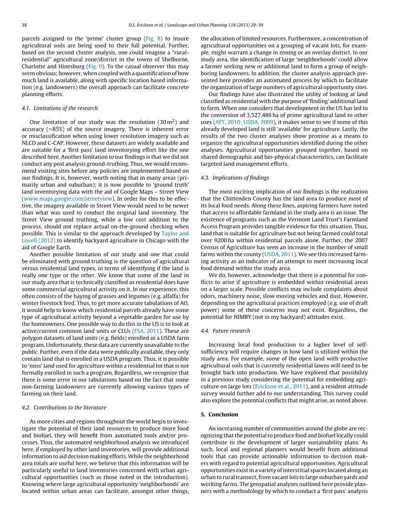

3 nd Ur

pabrCsmtp

4

aoNadcmoml(ttSppLa

bvrosowittapppctftnf

4

tachiapcKl

8 D.L. Erickson et al. / Landscape a

arcels assigned to the ‘prime’ cluster group (Fig. 8) to insuregricultural soils are being used to their full potential. Further,ased on the second cluster analysis, one could imagine a “rural-esidential” agricultural zone/district in the towns of Shelburne,harlotte and Hinesburg (Fig. 9). To the casual observer this mayeem obvious; however, when coupled with a quantification of howuch land is available, along with specific location based informa-

ion (e.g. landowners) the overall approach can facilitate concretelanning efforts.

.1. Limitations of the research

One limitation of our study was the resolution (30 m2) andccuracy (≈85%) of the source imagery. There is inherent errorr misclassification when using lower resolution imagery such asLCD and C-CAP. However, these datasets are widely available andre suitable for a ‘first pass’ land inventorying effort like the oneescribed here. Another limitation to our findings is that we did notonduct any post analysis ground-truthing. Thus, we would recom-end visiting sites before any policies are implemented based on

ur findings. It is, however, worth noting that in many areas (pri-arily urban and suburban); it is now possible to ‘ground truth’

and inventorying data with the aid of Google Maps – Street Viewwww.maps.google.com/streetview). In order for this to be effec-ive, the imagery available in Street View would need to be newerhan what was used to conduct the original land inventory. Thetreet View ground truthing, while a low cost addition to therocess, should not replace actual on-the-ground checking whenossible. This is similar to the approach developed by Taylor andovell (2012) to identify backyard agriculture in Chicago with theid of Google Earth.

Another possible limitation of our study and one that coulde eliminated with ground truthing is the question of agriculturalersus residential land types, in terms of identifying if the land iseally one type or the other. We know that some of the land inur study area that is technically classified as residential does haveome commercial agricultural activity on it. In our experience, thisften consists of the haying of grasses and legumes (e.g. alfalfa) forinter livestock feed. Thus, to get more accurate tabulations of AO,

t would help to know which residential parcels already have someype of agricultural activity beyond a vegetable garden for use byhe homeowners. One possible way to do this in the US is to look atctive/current common land units or CLUs (FSA, 2011). These areolygon datasets of land units (e.g. fields) enrolled in a USDA farmrogram. Unfortunately, these data are currently unavailable to theublic. Further, even if the data were publically available, they onlyontain land that is enrolled in a USDA program. Thus, it is possibleo ‘miss’ land used for agriculture within a residential lot that is notormally enrolled in such a program. Regardless, we recognize thathere is some error in our tabulations based on the fact that someon-farming landowners are currently allowing various types of

arming on their land.

.2. Contributions to the literature

As more cities and regions throughout the world begin to inves-igate the potential of their land resources to produce more foodnd biofuel, they will benefit from automated tools and/or pro-esses. Thus, the automated neighborhood analysis we introducedere, if employed by other land inventories, will provide additional

nformation to aid decision making efforts. While the neighborhoodrea totals are useful here, we believe that this information will be

articularly useful to land inventories concerned with urban agri-ultural opportunities (such as those noted in the introduction).nowing where large agricultural opportunity ‘neighborhoods’ are

ocated within urban areas can facilitate, amongst other things,

ban Planning 118 (2013) 29– 39

the allocation of limited resources. Furthermore, a concentration ofagricultural opportunities on a grouping of vacant lots, for exam-ple, might warrant a change in zoning or an overlay district. In ourstudy area, the identification of large ‘neighborhoods’ could allowa farmer seeking new or additional land to form a group of neigh-boring landowners. In addition, the cluster analysis approach pre-sented here provides an automated process by which to facilitatethe organization of large numbers of agricultural opportunity sites.

Our findings have also illustrated the utility of looking at landclassified as residential with the purpose of ‘finding’ additional landto farm. When one considers that development in the US has led tothe conversion of 3,527,486 ha of prime agricultural land to otheruses (AFT, 2010; USDA, 2009), it makes sense to see if some of thisalready developed land is still ‘available’ for agriculture. Lastly, theresults of the two cluster analyses show promise as a means toorganize the agricultural opportunities identified during the otheranalyses. Agricultural opportunities grouped together, based onshared demographic and bio-physical characteristics, can facilitatetargeted land management efforts.

4.3. Implications of findings

The most exciting implication of our findings is the realizationthat the Chittenden County has the land area to produce most ofits local food needs. Along these lines, aspiring farmers have notedthat access to affordable farmland in the study area is an issue. Theexistence of programs such as the Vermont Land Trust’s FarmlandAccess Program provides tangible evidence for this situation. Thus,land that is suitable for agriculture but not being farmed could totalover 9200 ha within residential parcels alone. Further, the 2007Census of Agriculture has seen an increase in the number of smallfarms within the county (USDA, 2011). We see this increased farm-ing activity as an indicator of an attempt to meet increasing localfood demand within the study area.

We do, however, acknowledge that there is a potential for con-flicts to arise if agriculture is embedded within residential areason a larger scale. Possible conflicts may include complaints aboutodors, machinery noise, slow moving vehicles and dust. However,depending on the agricultural practices employed (e.g. use of draftpower) some of these concerns may not exist. Regardless, thepotential for NIMBY (not in my backyard) attitudes exist.

4.4. Future research

Increasing local food production to a higher level of self-sufficiency will require changes in how land is utilized within thestudy area. For example, some of the open land with productiveagricultural soils that is currently residential lawns will need to bebrought back into production. We have explored that possibilityin a previous study considering the potential for embedding agri-culture on large lots (Erickson et al., 2011), and a resident attitudesurvey would further add to our understanding. This survey couldalso explore the potential conflicts that might arise, as noted above.

5. Conclusion

An increasing number of communities around the globe are rec-ognizing that the potential to produce food and biofuel locally couldcontribute to the development of larger sustainability plans. Assuch, local and regional planners would benefit from additionaltools that can provide actionable information to decision mak-ers with regard to potential agricultural opportunities. Agricultural

opportunities exist in a variety of interstitial spaces located along anurban to rural transect, from vacant lots to large suburban yards andworking farms. The geospatial analyses outlined here provide plan-ners with a methodology by which to conduct a ‘first pass’ analysis

nd Ur

ctdnrwtTbe

R

A

A

B

B

C

D

D

E

E

F

F

G

G

G

G

G

H

H

K

D.L. Erickson et al. / Landscape a

oncerned with identifying and quantifying these diverse agricul-ural opportunities. The cluster analyses provide an automated,ata driven means by which to begin to organize these opportu-ities. This approach has the advantage of being conducted moreapidly and on a larger scale than ‘on the ground’ land mappinghich has its own inherent limitations. The visuals associated with

hese analyses can provide a starting point for community planning.hese tools have the potential to facilitate participatory planningy bringing residents and farmers to the table with planners, in anffort to better plan for an unpredictable future.

eferences

FT. (2010). American farmland trust – farmland information center 2007 NRI:Changes in land cover/use – agricultural land. http://www.farmlandinfo.org/documents/38426/Final 2007 NRI Agricultural Land.pdf (Accessed 01.02.11.)

PA. (2010). American planning association – the land based classification standards(LBCS). http://www.planning.org/lbcs/ (Retrieved 12.08.10.)

almer, K., Gill, J., Kaplinger, H., Miller, J., Peterson, M., Rhoads, A., et al.(2005). The Diggable city: Making urban agriculture a planning priority.Portland State University, Hohad A. Toulan School of Urban Studies andPlanning.

oudjenouia, A., Fleury, A., & Tacherift, A. (2008). Suburban agriculture in Setif (Alge-ria): Which future in face of urban growth? Biotechnologie Agronomie Societe EtEnvironnement, 12(1), 23–30.

availhes, J., & Wavresky, P. (2003). Urban influences on periurban farmland prices.European Review of Agricultural Economics, 30(3), 333–357.

empsey, J., & Ferguson, K. (2010). Farmland by the numbers. American Farmland,Fall-Winter, 2010.

VRP.C. (2010). Greater Philadelphia Food System Study. Delaware Valley RegionalPlanning Commission.

dwards-Jones, G., Milà i Canals, L., Hounsome, N., Truninger, M., Koerber, G.,Hounsome, B., et al. (2008). Testing the assertion that ‘local food is best’: Thechallenges of an evidence-based approach. Trends in Food Science and Technology,19(5), 265–274. http://dx.doi.org/10.1016/j.tifs.2008.01.008

rickson, D. L., Lovell, S. T., & Méndez, V. E. (2011). Landowner willingnessto embed production agriculture and other land use options in residen-tial areas of Chittenden County, VT. Landscape and Urban Planning, 103,174–184.

azal, S. (2001). The need for preserving farmland – A case study from a pre-dominantly agrarian economy (India). Landscape and Urban Planning, 55(1),1–13.

SA. (2011). USDA – Farm services agency. Common Land Unit (CLU).http://www.fsa.usda.gov/FSA/apfoapp?area=home&subject=prod&topic=clu(Accessed 07.11.11.)

alvin, M. F., Grove, J. M., & O‘Neil-Dunne, J. P. M. (2006a). . A report on Annapoliscity’s present and potential urban tree canopy forest service (vol. 17) MarylandDepartment of Natural Resources.

alvin, M. F., Grove, J. M., & O‘Neil-Dunne, J. P. M. (2006b). . A report on Baltimorecity’s present and potential urban tree canopy forest service (vol. 17) MarylandDepartment of Natural Resources.

iner, N. M., Polsky, C., Pontius, R. G., & Runfola, D. M. (2013). Understanding thesocial determinants of lawn landscapes: A fine-resolution spatial statistical anal-ysis in suburban Boston, Massachusetts, USA. Landscape and Urban Planning,111(0), 25–33. http://dx.doi.org/10.1016/j.landurbplan.2012.12.006

rewal, S. S., & Grewal, P. S. (2012). Can cities become self-reliant in food? Cities,29(1), 1–11. http://dx.doi.org/10.1016/j.cities.2011.06.003

rove, J. M., O‘Neil-Dunne, J. P. M., Pelletier, K., Nowak, D. J., & Walton, J. (2006).A report on New York city’s present and possible urban tree canopy. NorthernResearch Station, USDA Forest Service.

eimlich, R. E., & Anderson, W. D. (2001). Development at the urban fringe and beyond:Impacts on agriculture and rural land. Economic Research Service, U.S. Depart-ment of Agriculture. Agricultural economic report no. 803.

orst, M. (2008). Growing green: An inventory of public lands suitable for community

gardening in Seattle. Washington: University of Washington, College of Archi-tecture and Urban Planning.

aethler, T. M. (2006). Growing space: The potential for urban agriculture in the city ofVancouver. University of British Columbia, School of Community and RegionalPlanning.

ban Planning 118 (2013) 29– 39 39

Kremer, P., & DeLiberty, T. L. (2011). Local food practices and growing poten-tial: Mapping the case of Philadelphia. Applied Geography, 31(4), 1252–1261.http://dx.doi.org/10.1016/j.apgeog.2011.01.007

MacRae, R., Gallant, E., Patel, S., Michalak, M., Bunch, M., & Schaffner, S. (2010).Could Toronto provide 10% of its fresh vegetable requirements from within itsown boundaries? Matching consumption requirements with growing spaces.Journal of Agriculture, Food Systems, and Community Development, 1(2), 105–127.http://dx.doi.org/10.5304/jafscd.2010.012.008

Matteucci, S. D., & Morello, J. (2009). Environmental consequences of exurban expan-sion in an agricultural area: The case of the Argentinian Pampas ecoregion[electronic resource]. Urban Ecosystems, 12(3), 287–310.

McClintock, N., & Cooper, J. (2010). Cultivating the commons an assessment of thepotential for urban agriculture on Oakland’s public land. Berkeley: Department ofGeography, University of California.

McClintock, N., Cooper, J., & Khandeshi, S. (2013). Assessing the potentialcontribution of vacant land to urban vegetable production and consump-tion in Oakland, California. Landscape and Urban Planning, 111, 46–58.http://dx.doi.org/10.1016/j.landurbplan.2012.12.009

McKellips, B. (2009). Laying the groundwork: A snapshot of a regional food system inChittenden and surrounding counties. Burlington, VT: The Intervale Center.

Mendes, W., Balmer, K., Kaethler, T., & Rhoads, A. (2008). Using land inventoriesto plan for urban agriculture experiences from Portland and Vancou-ver. [Article]. Journal of the American Planning Association, 74(4), 435–449.http://dx.doi.org/10.1080/01944360802354923

NOAA. (2011). Coastal Change Analysis Program Regional Land Cover.http://csc.noaa.gov/digitalcoast/data/ccapregional (accessed 11.11.11)

Plantinga, A. J., Lubowski, R. N., & Stavins, R. N. (2002). The effects of potential landdevelopment on agricultural land prices. [Article]. Journal of Urban Economics,52(3), 561–581.

Plantinga, A. J., & Miller, D. J. (2001). Agricultural land values and the value of rightsto future land development [Article]. Land Economics, 77(1), 56–67.

Polimeni, J. M. (2005). Simulating agricultural conversion to residential use in theHudson River Valley: Scenario analyses and case studies. Agriculture and HumanValues, 22(4), 377–393. http://dx.doi.org/10.1007/s10460-005-3389-5

Raciti, S., Galvin, M. F., Grove, J. M., O‘Neil-Dunne, J. P. M., Todd, A., & Clagett, S.(2006). Urban tree canopy goal setting a guide for Chesapeake Bay communities.USDA Forest Service., 59.

Risku-Norja, H., Hietala, R., Virtanen, H., Ketomaki, H., & Helenius, J. (2008).Localisation of primary food production in Finland: Production potential andenvironmental impacts of food consumption patterns. Agricultural and Food Sci-ence, 17(2), 127–145. http://dx.doi.org/10.2137/145960608785328233

Taggart, M., Chaney, M., Meaney, D., & Land Use & Planning Working Group. (2009).Cleveland Area vacant land inventory for urban agriculture – Report for urban landecology conference. Cleveland: Cuyahoga County Food Policy Coalition.

Taylor, J. R., & Lovell, S. T. (2012). Mapping public and private spaces of urban agricul-ture in Chicago through the analysis of high-resolution aerial images in GoogleEarth. Landscape and Urban Planning, 108(1), 57–70.

Thapa, R. B., & Murayama, Y. (2008). Land evaluation for peri-urban agricul-ture using analytical hierarchical process and geographic information systemtechniques: A case study of Hanoi [Article]. Land Use Policy, 25(2), 225–239.http://dx.doi.org/10.1016/j.landusepol.2007.06.004

USCB. (2011). Chittenden County quick facts from the US Census Bureau.http://quickfacts.census.gov/qfd/states/50/50007.html (Accessed 11.11.11)

USCB. (2013). State median income. http://www.census.gov/hhes/www/income/data/statemedian/ (Retrieved 11.03.13.)

USDA. (2009). Summary Report 2007 National Resources Inventory. Ames,Iowa: Natural Resources Conservation Service, Washington, DC/Centerfor Survey Statistics and Methodology, Iowa State University. IowaState University – Center for Survey Statistics and Methodology,http://www.nrcs.usda.gov/technical/NRI/2007/2007 NRI Summary.pdf

USDA. (2011). 2007 census of agriculture – county profile – Chittenden County VT.http://www.agcensus.usda.gov/Publications/2007/Online Highlights/CountyProfiles/Vermont/cp50007.pdf. (Retrieved 14.11.11.)

V.S.J.F. (2011). Vermont Sustainable Jobs Fund. In Farm to plate: A 10-year strategic plan for Vermont’s food system. Executive summary.http://www.vsjf.org/assets/files/Agriculture/Strat Plan/F2P%20Executive%20Summary 6.27.11 Small%20File.pdf (Accessed 17.10.11.)

VTDoE. (2012). Child nutrition programs – Annual statistical report – Percent of students

eligible for free and reduced price school meals school year 2010–2011. VermontDepartment of Education.

Yan, H. M., Liu, J. Y., Huang, H. Q., Tao, B., & Cao, M. K. (2009). Assessing the conse-quence of land use change on agricultural productivity in China. Global and Plane-tary Change, 67(1–2), 13–19. http://dx.doi.org/10.1016/j.gloplacha.2008.12.012