Embed Size (px)
Citation preview
LANDSCAPE & BUILDING SOLAR LOADS:
DEVELOPMENT OF A COMPUTER BASED TOOL TO AID IN THE DESIGN OF
LANDSCAPE TO REDUCE SOLAR GAIN AND ENERGY CONSUMPTION IN
LOW-RISE RESIDENTIAL BUILDINGS
by
Aran Morrow Osborne
A Thesis Presented to the FACULTY OF THE SCHOOL OF ARCHITECTURE
UNIVERSITY OF SOUTHERN CALIFORNIA In Partial Fulfilment of the
Requirements for the Degree MASTER OF BUILDING SCIENCE
August 2009
Copyright 2009 Aran Morrow Osborne

UMI Number: 1467522
Copyright 2009 by Osborne, Aran Morrow
All rights reserved
INFORMATION TO USERS
The quality of this reproduction is dependent upon the quality of the copy
submitted. Broken or indistinct print, colored or poor quality illustrations and
photographs, print bleed-through, substandard margins, and improper
alignment can adversely affect reproduction.
In the unlikely event that the author did not send a complete manuscript
and there are missing pages, these will be noted. Also, if unauthorized
copyright material had to be removed, a note will indicate the deletion.
______________________________________________________________
UMI Microform 1467522Copyright 2009 by ProQuest LLC
All rights reserved. This microform edition is protected against unauthorized copying under Title 17, United States Code.
_______________________________________________________________
ProQuest LLC 789 East Eisenhower Parkway
P.O. Box 1346 Ann Arbor, MI 48106-1346

ii
EPIGRAPH
It may be that some little root of the Sacred Tree still lives. Nourish it then, that it may leaf and bloom and fill with singing birds. Hear me, not for myself, but for my people… Hear me that they may once more go back into the Sacred Hoop and find the good red road, the shielding tree. - Black Elk

iii
ACKNOLWEDGEMENTS
Several people contributed their time and energy toward the development and
completion of this thesis. I would like to extend my many thanks to Professor
Thomas Spiegelhalter for his guidance and enthusiasm; to Professor Marc Schiler for
his extensive knowledge and support during program completion; to Professor Karen
Kensek for her invaluable suggestions during program development and verification;
to Kimberly Wiebe for helping me learn Visual Basic; and to my fellow Master of
Building Science and Architecture students for helping to make my experience at the
University of California an unforgettable one.
I would also like to send much love and thanks to my parents, Don and Gail; to my
sister, Jaime; to Rafaela; and to all my friends for their support throughout my time
at USC.
iv
TABLE OF CONTENTS
EPIGRAPH ii
ACKNOLWEDGEMENTS iii
LIST OF TABLES vii
LIST OF FIGURES viii
ABSTRACT xiii
CHAPTER 1 1
1.1 Introduction 1 1.2 Hypothesis Statement 1 1.3 Importance 2 1.4 Study Boundaries 6 1.5 Scope of Work 6
CHAPTER 2 8
2.1 Microclimatic Landscape Design 8 2.1.1 Macroclimatology 9 2.1.2 Landscape and the Microclimate 9 2.1.3 Landscaping for the Microclimate 11
2.2 Potential of Landscape to Reduce Heating/Cooling Loads in Buildings 14 2.3 Calculating Heating and Cooling Loads 16
2.3.1 Principles of Heat Transfer 16 2.3.2 Cooling Loads 22
2.4 Shading 27 2.4.1 Solar Radiation 27 2.4.2 Terrestrial Radiation 30 2.4.3 Radiation and Plants 30 2.4.4 Calculating Cooling Effects of Tree Shade 32 2.4.5 Previous Studies 33
2.5 Wind Breaks 37 2.5.1 Wind 37 2.5.2 Effect of Plants on Wind 40 2.5.3 Calculating Energy Saving Potential of Wind Breaks 45 2.5.3 Previous Studies 47
2.6 Evapotranspiration 49 2.6.1 Calculating Evapotranspiration 50 2.6.2 Previous Studies 54
2.7 Effect of Trees on the Urban Heat Island 58 2.8 Energy-Efficient Residential Landscape – Design Approaches 61
2.8.1 Hot, Arid Climates 62 2.8.2 Hot, Humid Climates 64 2.8.3 Temperate Climates 66 2.8.4 Cool Climates 68
2.9 Landscape Elements 71 2.9.1 California Climate Zones 71 2.9.2 Native Vegetation 73
v
CHAPTER 3 75
3.1 Instantaneous Cooling Load Calculation 75 3.2 Shading – Algorithm and Savings Calculations 77
3.2.1 Equations for Solar Azimuth and Altitude Angles 77 3.2.2 Determining Plane for Shading Calculation 79 3.2.3 Projection of Shade Pattern onto Wall Plane 83 3.2.4 Calculating Savings from Shading 83
3.3 Wind Breaks 85 3.4 Evapotranspiration 85 3.5 Tree Library and Database 86
3.5.1 Vegetation Habitats 86 3.5.2 Tree Database Development 89
CHAPTER 4 91
4.1 What The Tool Does 91 4.2 Visual Basic 91 4.3 Development Approach 92
4.3.1 Scope 93 4.3.2 Requirements 94 4.3.3 Design 96 4.3.4 Code 99 4.4.1 Screen 1 – Welcome Screen 104 4.4.2 Screen 2 – Building Information 108 4.4.3 Screens 3, 4 & 5 – Fenestration 109 4.4.4 Screen 6 – Tree Selection 110 4.4.5 Screen 7 - Tree Placement 113 4.4.6 Scanline Algorithm & Instantaneous Cooling Load Calculations 116 4.4.6 Screen 9 – Savings Output Screen 120
CHAPTER 5 122
5.1 Verification of Program Code 122 5.1.1 Verification of Tree Polygon Construction Code 122 5.1.2 Verification of Scanline Algorithm Code 124 5.1.3 Verification of Matrix Transformations 126 5.1.4 Verification of Transmissivity Multiplier 128
5.2 Comparison to HEED 130 5.2.1 Overview of HEED 130 5.2.2 Comparison of Thesis Program to HEED 131 5.2.3 Thesis Program and HEED Inputs 132 5.2.4 Comparison of Outputs for East Window 134 5.2.5 Comparison of Outputs For South Window 143 5.2.6 Comparison of Outputs for West Window 145
5.3 Comparison to ECOTECT 148 5.3.1 Overview of ECOTECT 148 5.3.2 Thesis Program and Ecotect Inputs 153 5.3.3 Comparison of Outputs 155
vi
CHAPTER 6 167
6.1 Comparison to Previous Research Publications 167 6.1.1 Previous Research Comparison 1 167 6.1.2 Previous Research Comparison 2 170 6.1.3 Previous Research Comparison 3 172
6.2 Conclusions Regarding Published Research Comparisons 176 6.3 Overall Conclusions 176
CHAPTER 7 180
7.1 Increasing Geographical Boundaries 180 7.2 Increasing Tree Library & Including Other Landscape Elements 181 7.3 Expanding Sun Shading Analysis 181 7.4 Including Wind Break Analysis 182 7.5 Including Evapotranspirative Cooling Analysis 182 7.6 User Interface 183 7.7 Integration into Existing Software 183 7.8 Increased Boundary of Analysis 184 7.9 Improvement of Program Code 184 7.10 Cost and Payback Analysis 185 7.11 Additional Verification Analysis 185
BIBLIOGRAPHY 186
APPENDICES 191
APPENDIX A: TREE LIBRARY DATA 191 APPENDIX B: PROGRAM CODE 192 APPENDIX C: SCANLINE ALGORITHM VERIFICATION 280 APPENDIX D: HEED VS. PROGRAM – UNSHADED 12-DAY AND SINGLE DAY ENERGY GAIN ANALYSIS 284
vii
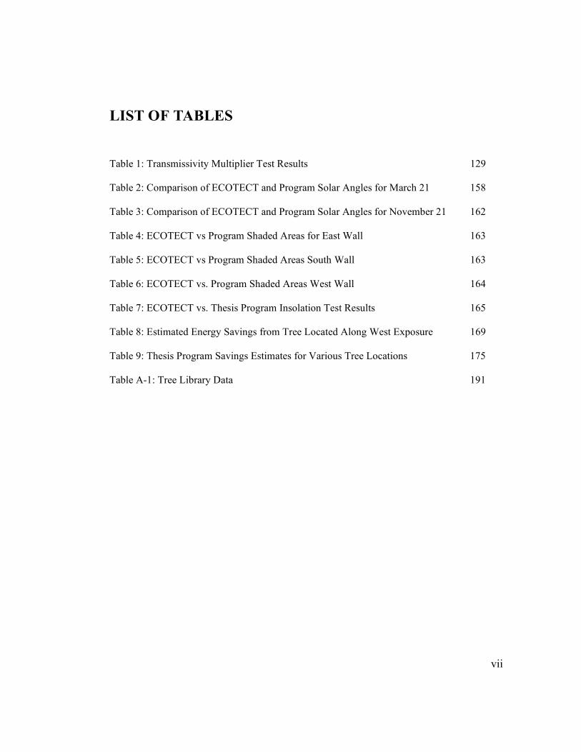
LIST OF TABLES
Table 1: Transmissivity Multiplier Test Results 129
Table 2: Comparison of ECOTECT and Program Solar Angles for March 21 158
Table 3: Comparison of ECOTECT and Program Solar Angles for November 21 162
Table 4: ECOTECT vs Program Shaded Areas for East Wall 163
Table 5: ECOTECT vs Program Shaded Areas South Wall 163
Table 6: ECOTECT vs. Program Shaded Areas West Wall 164
Table 7: ECOTECT vs. Thesis Program Insolation Test Results 165
Table 8: Estimated Energy Savings from Tree Located Along West Exposure 169
Table 9: Thesis Program Savings Estimates for Various Tree Locations 175 Table A-1: Tree Library Data 191
viii
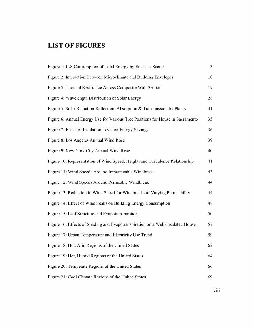
LIST OF FIGURES
Figure 1: U.S Consumption of Total Energy by End-Use Sector 3
Figure 2: Interaction Between Microclimate and Building Envelopes 10
Figure 3: Thermal Resistance Across Composite Wall Section 19
Figure 4: Wavelength Distribution of Solar Energy 28
Figure 5: Solar Radiation Reflection, Absorption & Transmission by Plants 31
Figure 6: Annual Energy Use for Various Tree Positions for House in Sacramento 35
Figure 7: Effect of Insulation Level on Energy Savings 36
Figure 8: Los Angeles Annual Wind Rose 39
Figure 9: New York City Annual Wind Rose 40
Figure 10: Representation of Wind Speed, Height, and Turbulence Relationship 41
Figure 11: Wind Speeds Around Impermeable Windbreak 43
Figure 12: Wind Speeds Around Permeable Windbreak 44
Figure 13: Reduction in Wind Speed for Windbreaks of Varying Permeability 44
Figure 14: Effect of Windbreaks on Building Energy Consumption 48
Figure 15: Leaf Structure and Evapotranspiration 50
Figure 16: Effects of Shading and Evapotranspiration on a Well-Insulated House 57
Figure 17: Urban Temperature and Electricity Use Trend 59
Figure 18: Hot, Arid Regions of the United States 62
Figure 19: Hot, Humid Regions of the United States 64
Figure 20: Temperate Regions of the United States 66
Figure 21: Cool Climate Regions of the United States 69
ix
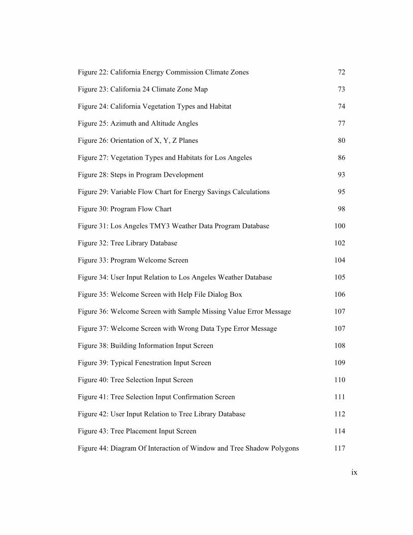
Figure 22: California Energy Commission Climate Zones 72
Figure 23: California 24 Climate Zone Map 73
Figure 24: California Vegetation Types and Habitat 74
Figure 25: Azimuth and Altitude Angles 77
Figure 26: Orientation of X, Y, Z Planes 80
Figure 27: Vegetation Types and Habitats for Los Angeles 86
Figure 28: Steps in Program Development 93
Figure 29: Variable Flow Chart for Energy Savings Calculations 95
Figure 30: Program Flow Chart 98
Figure 31: Los Angeles TMY3 Weather Data Program Database 100
Figure 32: Tree Library Database 102
Figure 33: Program Welcome Screen 104
Figure 34: User Input Relation to Los Angeles Weather Database 105
Figure 35: Welcome Screen with Help File Dialog Box 106
Figure 36: Welcome Screen with Sample Missing Value Error Message 107
Figure 37: Welcome Screen with Wrong Data Type Error Message 107
Figure 38: Building Information Input Screen 108
Figure 39: Typical Fenestration Input Screen 109
Figure 40: Tree Selection Input Screen 110
Figure 41: Tree Selection Input Confirmation Screen 111
Figure 42: User Input Relation to Tree Library Database 112
Figure 43: Tree Placement Input Screen 114
Figure 44: Diagram Of Interaction of Window and Tree Shadow Polygons 117
x
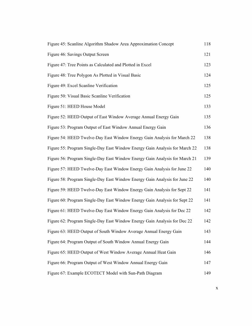
Figure 45: Scanline Algorithm Shadow Area Approximation Concept 118
Figure 46: Savings Output Screen 121
Figure 47: Tree Points as Calculated and Plotted in Excel 123
Figure 48: Tree Polygon As Plotted in Visual Basic 124
Figure 49: Excel Scanline Verification 125
Figure 50: Visual Basic Scanline Verification 125
Figure 51: HEED House Model 133
Figure 52: HEED Output of East Window Average Annual Energy Gain 135
Figure 53: Program Output of East Window Annual Energy Gain 136
Figure 54: HEED Twelve-Day East Window Energy Gain Analysis for March 22 138
Figure 55: Program Single-Day East Window Energy Gain Analysis for March 22 138
Figure 56: Program Single-Day East Window Energy Gain Analysis for March 21 139
Figure 57: HEED Twelve-Day East Window Energy Gain Analysis for June 22 140
Figure 58: Program Single-Day East Window Energy Gain Analysis for June 22 140
Figure 59: HEED Twelve-Day East Window Energy Gain Analysis for Sept 22 141
Figure 60: Program Single-Day East Window Energy Gain Analysis for Sept 22 141
Figure 61: HEED Twelve-Day East Window Energy Gain Analysis for Dec 22 142
Figure 62: Program Single-Day East Window Energy Gain Analysis for Dec 22 142
Figure 63: HEED Output of South Window Average Annual Energy Gain 143
Figure 64: Program Output of South Window Annual Energy Gain 144
Figure 65: HEED Output of West Window Average Annual Heat Gain 146
Figure 66: Program Output of West Window Annual Energy Gain 147
Figure 67: Example ECOTECT Model with Sun-Path Diagram 149

xi
Figure 68: Example ECOTECT Model View From the Sun 150
Figure 69: ECOTECT Shading Casting Example 151
Figure 70: ECOTECT Sun View Shading Casting Example 151
Figure 71: ECOTECT House Model 154
Figure 72: Excel Sun View of East-Facing Wall at 9:00 am 156
Figure 73: ECOTECT Sun View of East-Facing Wall at 9:00 am 156
Figure 74: Excel Sun View of South-Facing Wall at 9:00 am 156
Figure 75: ECOTECT Sun View of South-Facing Wall at 9:00 am 156
Figure 76: Excel Sun View of South-Facing Wall at 4:00 pm 156
Figure 77: ECOTECT Sun View of South-Facing Wall at 4:00 pm 156
Figure 78: Excel Sun View of West-Facing Wall at 4:00 pm 157
Figure 79: ECOTECT Sun View of West-Facing Wall at 4:00 pm 157
Figure 80: Excel 2D Polygon Projection on November 21 at 9:00 am 160
Figure 81: ECOTECT 2D Polygon Projection on November 21 at 9:00 am 160
Figure 82: Excel 2D Polygon Projection on November 21 at 12:00 pm 160
Figure 83: ECOTECT 2D Polygon Projection on November 21 at 12:00 pm 160
Figure 84: Excel 2D Polygon Projection on November 21 at 2:00 pm 160
Figure 85: ECOTECT 2D Polygon Projection on November 21 at 2:00 pm 160
Figure 86: Excel 2D Polygon Projection on June 21 at 12:00 pm 161
Figure 87: ECOTECT 2D Polygon Projection on June 21 at 12:00 pm 161
Figure 88: Air-Conditioning Savings from Landscape for Selected U.S Cities 168
Figure C-1: Excel Scanline Verification Test 2 280
Figure C-2: Visual Basic Scanline Verification Test 2 280

xii
Figure C-3: Excel Scanline Verification Test 3 281
Figure C-4: Visual Basic Scanline Verification Test 3 281
Figure C-5: Excel Scanline Verification Test 4 282
Figure C-6: Visual Basic Scanline Verification Test 4 282
Figure C-7: Excel Scanline Verification Test 5 283
Figure C-8: Visual Basic Scanline Verification Test 5 283
Figure D-1: HEED Twelve-Day South Window Energy Gain Analysis for March 284
Figure D-2: Program Single-Day South Window Energy Gain Analysis for March 284
Figure D-3: HEED Twelve-Day South Window Energy Gain Analysis for June 285
Figure D-4: Program Single-Day South Window Energy Gain Analysis for June 285
Figure D-5: HEED Twelve-Day South Window Energy Gain Analysis for Sept 286
Figure D-6: Program Single-Day South Window Energy Gain Analysis for Sept 286
Figure D-7: HEED Twelve-Day South Window Energy Gain Analysis for Dec 287
Figure D-8: Program Single-Day South Window Energy Gain Analysis for Dec 287
Figure D-9: HEED Twelve-Day West Window Energy Gain Analysis for March 288
Figure D-10: Program Single-Day West Window Energy Gain Analysis for March 288
Figure D-11: HEED Twelve-Day West Window Energy Gain Analysis for June 289
Figure D-12: Program Single-Day West Window Energy Gain Analysis for June 289
Figure D-13: HEED Twelve-Day West Window Energy Gain Analysis for Sept 290
Figure D-14: Program Single-Day West Window Energy Gain Analysis for Sept 290
Figure D-15: HEED Twelve-Day West Window Energy Gain Analysis for Dec 291
Figure D-16: Program Single-Day West Window Energy Gain Analysis for Dec 291
xiii
ABSTRACT
The aim of this project was to develop a computer-based simulation tool to provide
information on landscape design that could be implemented to help reduce solar gain
and energy consumption in low-rise residential buildings. The program recommends
specific landscape design strategies based on user inputs and also outputs potential
energy savings should the strategies be applied. Literature review was performed to
obtain information regarding the potential benefits of landscape design on building
loads and energy performance and also to determine what information would be
required to recommend an effective landscape design. Published equations and data
as well as previous programming approaches were referenced to help form the
program algorithms. Software such as MATLAB, Microsoft Excel, HEED, and
ECOTECT were used in the verification of program code, equations, and outputs.
Comparisons to previous research publications were also used in the validation of the
program calculations. The results of the verification and validation demonstrated
that expected savings outputs were acceptable and that the program functioned as
intended. The final result is a freestanding Visual Basic program that can be
effectively and accurately used in the development of energy-efficient landscape
designs.
1
CHAPTER 1
1.1 INTRODUCTION
Diminishing resources and increasing fuel prices continue to drive the need for
greater energy efficiency and more effective conservation strategies, especially in
buildings. Resources are typically funnelled into researching technological
solutions; however plants and their innate ability to reduce the energy demand in
adjacent buildings are often overlooked. Extensive research has been conducted
regarding the ability of plants to reduce solar heat gain into buildings, provide
cooling through evapotranspiration, and also to help prevent convective heat loss by
acting as wind breaks. This thesis seeks to investigate the effects of landscape on
low-rise, residential buildings, and compile this information into a simple, computer-
based tool. The purpose of the tool will be to analyze a specific building, in terms of
location and construction data, and provide landscape design suggestions along with
corresponding energy and cost savings that could be achieved.
1.2 HYPOTHESIS STATEMENT
It is possible to develop a computer-based tool that, when provided with inputs from
the user, can
2
1) Recommend specific landscape design strategies for low-rise residential
buildings that can potentially reduce energy consumption within the
building, and
2) Output potential energy and cost savings should the landscape strategies be
implemented.
1.3 IMPORTANCE
Global warming, resource depletion and, in general, the environmental crisis are
growing concerns in contemporary society. Mounting scientific evidence clearly
demonstrates the need for humans to change the manner in which we live, build, and
use resources. Although much current attention is aimed at automobiles with their
high rate of fuel consumption and production of green house gases, a U.S
Department of Energy survey published in 2007 reports that transportation represents
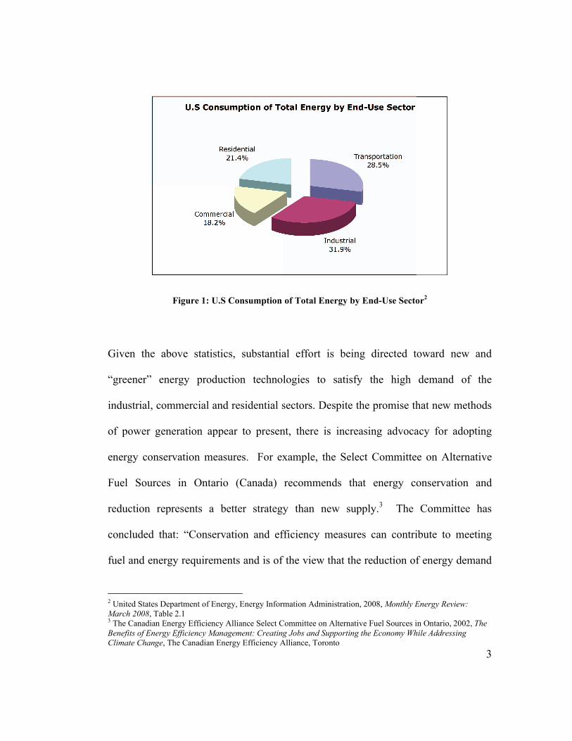
only 28.5% of total energy consumption by end-use sector. The same survey reports
industrial consumption at 31.9%, commercial consumption at 18.1%, and residential
consumption at 21.4%.1 See Figure 1 below.
1 United States Department of Energy, Energy Information Administration, 2008, Monthly Energy Review:
March 2008, United States Department of Energy, Washington, DC
3
Figure 1: U.S Consumption of Total Energy by End-Use Sector2
Given the above statistics, substantial effort is being directed toward new and
“greener” energy production technologies to satisfy the high demand of the
industrial, commercial and residential sectors. Despite the promise that new methods
of power generation appear to present, there is increasing advocacy for adopting
energy conservation measures. For example, the Select Committee on Alternative
Fuel Sources in Ontario (Canada) recommends that energy conservation and
reduction represents a better strategy than new supply.3 The Committee has
concluded that: “Conservation and efficiency measures can contribute to meeting
fuel and energy requirements and is of the view that the reduction of energy demand
2 United States Department of Energy, Energy Information Administration, 2008, Monthly Energy Review:
March 2008, Table 2.13 The Canadian Energy Efficiency Alliance Select Committee on Alternative Fuel Sources in Ontario, 2002, The
Benefits of Energy Efficiency Management: Creating Jobs and Supporting the Economy While Addressing
Climate Change, The Canadian Energy Efficiency Alliance, Toronto
4
is more important than new supply.”4 Demand-side energy management is of vital
importance in energy conservation throughout North America. As another example,
the United States government recently adopted an initiative to weatherize one million
homes annually, as well as to reduce greenhouse gas emissions by 80% by the year
2050.5 Since buildings account for roughly half of total green house gas emissions in
the United States, focusing efforts on reduction of energy consumption at the
residential level can contribute significantly to achieving these objectives.
In the United States, buildings account for roughly 40% of total energy consumption,
with residential buildings comprising about 55% of that total.6 While only a portion
of this percentage is attributable to low-rise residential buildings, over 50% of the
American population live in suburban locations characterized by the detached,
single-family house.7 Such dwellings are typically isolated on large building lots and
are not often constructed using climate appropriate architecture or sustainable design.
Substantial information is now available for owners recommending the replacement
or retrofit of mechanical heating/cooling systems, lighting, appliances, as well as
renovating the architectural aspects of their homes (such as windows) in order to
lower energy consumption. Comparatively less information, however, is provided
4 The Canadian Energy Efficiency Alliance Select Committee on Alternative Fuel Sources in Ontario, The
Benefits of Energy Efficiency Management: Creating Jobs and Supporting the Economy While Addressing
Climate Change, 3 5 The White House, 2008, Energy & Environment, viewed September 2008, http://www.whitehouse.gov/issues/energy_and_environment/ 6 U.S Environmental Protection Agency Green Building Workgroup, 2004, Buildings and the Environment: A
Statistical Survey, United States Environmental Protection Agency, viewed September 2008, http://www.epa.gov/greenbuilding/pubs/gbstats.pdf 7 Rutherford H. Platt, The Humane Metropolis (University of Massachusetts Press, 2006), 12

5
regarding the potential for achieving savings via intelligent site design and
landscape. In addition to savings, the importance of landscaping with native and
adapted plants is also becoming widely acknowledged. For example, the Leadership
in Energy and Environmental Design (LEED) ratings systems for New Construction
as well as New Development award credits for the use of native plants in
landscaping.8 By incorporating native plants in energy efficient landscape design,
excessive irrigation requirements can also be avoided, which further contributes to
potential savings.
Landscaping to reduce energy consumption within a building can have considerable
impact on the performance of the house. Extensive research has been performed and
several publications have been produced that outline design guidelines and the
potential savings that can be achieved. Although such information exists, it is not
widely discussed or presented as a viable option to typical homeowners, and existing
publications are not always readily available in local bookstores or community
libraries. Computers and the Internet, however, are present and easily accessible in
roughly half of American homes today.9
A computer-based information and simulation tool, designed for homeowners who
have little or no knowledge of landscape or energy-efficient site design, would be a
8 United States Green Building Council, 2008, LEED Rating Systems, United States Gren Building Council, viewed September 2008, http://www.usgbc.org/DisplayPage.aspx?CMSPageID=222 9 United States Census Bureau, 2000, Home Computers and Internet Use in the United States, United States Census Bureau, viewed September 2008, http://www.census.gov/population/www/socdemo/computer.html
6
valuable resource for individuals who seek to adopt alternative and passive strategies
around their property. A tool that prompts for simple inputs and provides concise and
instructive outputs can provide information to homeowners regarding climate
appropriate landscape strategies that can potentially reduce building energy
consumption.
1.4 STUDY BOUNDARIES
The tool focuses on existing low-rise residential buildings in the United States.
Specifically, one-story, single-family, detached homes are included in the scope of
the tool. The tool is not designed for analysis of landscape for high-rise buildings.
The program could be expanded to include tract or row housing. The boundary for
program development will be limited to the hot, arid climate of Los Angeles, but it is
anticipated that the tool could be expanded to include all climate zones across the
United States. Furthermore, the tool is intended for private use of individual
homeowners. This focus was selected as it was concluded, from information
provided above, that the suburban housing residential sector represents a substantial
area for reducing energy consumption.
1.5 SCOPE OF WORK
The intention of this thesis is to develop a computer-based tool that will prompt the
user for a specific set of inputs regarding the location, site, and construction of the

7
house and then provide recommendations for the type of tree or vegetation that
should be used and where to place it in relation to the house to achieve energy
savings. The program also provides the user with expected energy and cost savings
should the design suggestions be implemented. The final product will be a
freestanding Visual Basic program that can be downloaded from the Internet and
which will run on the Windows Platform.
8
CHAPTER 2
2.1 MICROCLIMATIC LANDSCAPE DESIGN
Microclimatic landscape design is the practice of manipulating objects in the
surrounding area to alter the local environmental conditions. The practice is mostly
employed to improve human comfort within a space, but can also be used to alter
exterior conditions in order to improve internal building conditions (thus reducing
energy use required to maintain occupant comfort).
A microclimate is described by a set of conditions for solar and terrestrial radiation,
wind, air temperature, humidity, and precipitation in a small outdoor space.10 It is
usually on the scale of meters to tens of meters, unlike climate (or macroclimate),
which generally refers to meteorological conditions that prevail over a period of time
in a large region of hundreds of kilometres.11 Effective microclimatic landscape
design requires knowledge of these prevailing climate conditions as well as an
understanding of the ways in which objects in the landscape effect site conditions to
create microclimates.12
The following chapter discusses, in detail, the theory and methods of manipulating
microclimatic conditions through landscape design.
10 Robert D. Brown and Terry J. Gillespie, Microclimatic Landscape Design (Wiley, 1995), 1 11 ibid., 18 12 ibid., 2
9
2.1.1 MACROCLIMATOLOGY
The study and documentation of a particular climate region over a period of time is
known as macroclimatology, and it allows for the development of a set of climate
data. Such data records the variation in temperature, precipitation, incident solar
radiation, and many other variables that define the climatic or weather characteristics
and patterns of a particular region. These data often correlate to a given climate zone,
which in turn has a particular set of landscape design principles appropriate to the
occurring weather variations. These design guidelines are discussed in further detail
in section 2.7 below.
2.1.2 LANDSCAPE AND THE MICROCLIMATE
Unlike macroclimates, the specific microclimate of a location can be altered and
manipulated by various landscape elements within the space. That is, the prevailing
climate of an area interacts with objects in a landscape to create microclimates.13
These interactions can have effects on air temperature, wind velocity, solar radiation,
and relative humidity; and can strongly influence the thermal comfort of people
within a landscape as well as affect the energy required to heat and/or cool a
building.14
13 Brown et al., Microclimatic Landscape Design, 3 14 ibid., 3
10
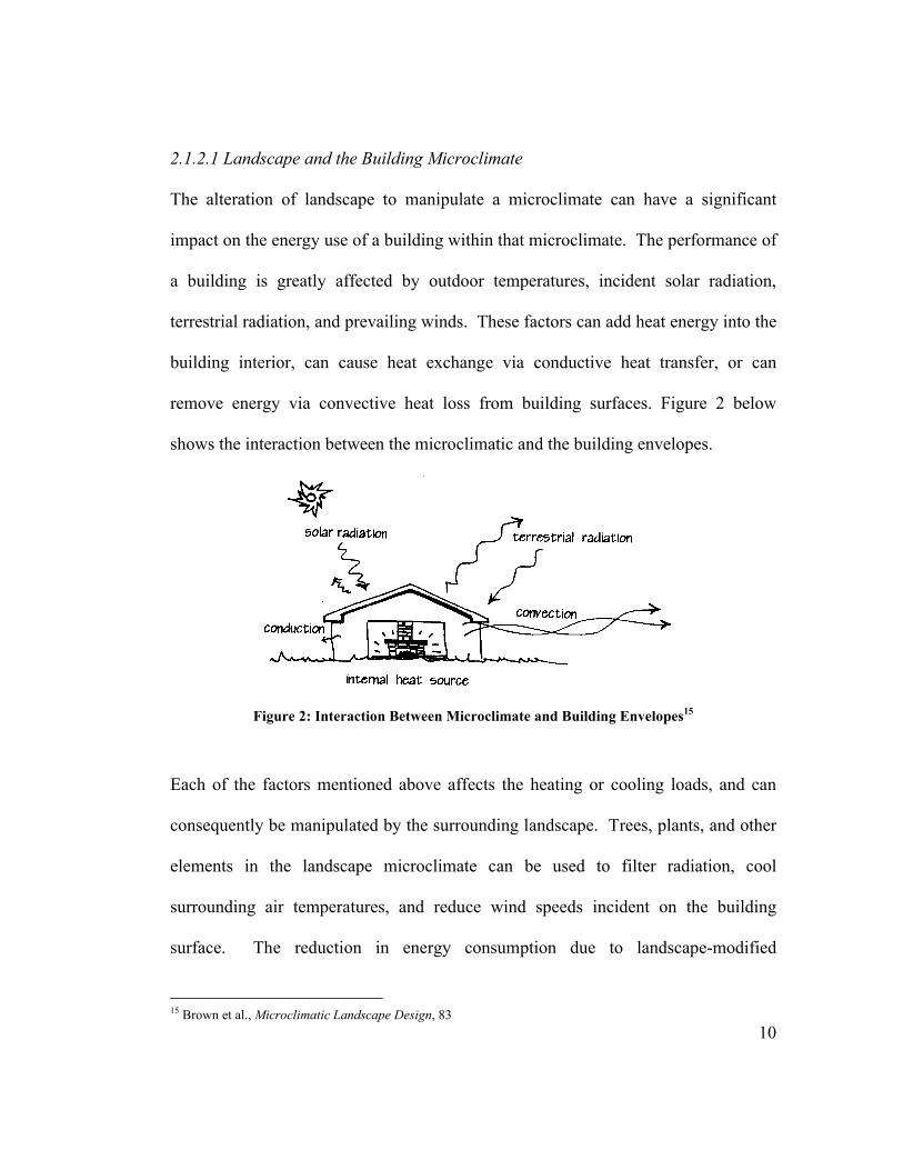
2.1.2.1 Landscape and the Building Microclimate
The alteration of landscape to manipulate a microclimate can have a significant
impact on the energy use of a building within that microclimate. The performance of
a building is greatly affected by outdoor temperatures, incident solar radiation,
terrestrial radiation, and prevailing winds. These factors can add heat energy into the
building interior, can cause heat exchange via conductive heat transfer, or can
remove energy via convective heat loss from building surfaces. Figure 2 below
shows the interaction between the microclimatic and the building envelopes.
Figure 2: Interaction Between Microclimate and Building Envelopes15
Each of the factors mentioned above affects the heating or cooling loads, and can
consequently be manipulated by the surrounding landscape. Trees, plants, and other
elements in the landscape microclimate can be used to filter radiation, cool
surrounding air temperatures, and reduce wind speeds incident on the building
surface. The reduction in energy consumption due to landscape-modified
15 Brown et al., Microclimatic Landscape Design, 83
11
microclimates is dependent on the construction of the building: well-insulated,
airtight buildings will benefit the least, while poorly insulated buildings will benefit
the most.16
2.1.3 LANDSCAPING FOR THE MICROCLIMATE
As mentioned in the previous section, a landscape can have a strong influence on the
prevailing conditions in a microclimate. As such, appropriate microclimate design
requires 1) knowledge of prevailing climate conditions, 2) understanding of the ways
in which objects in the landscape affect climate to create microclimates, and 3)
methods for applying this knowledge, through landscape design, to create
microclimates that are comfortable for people and minimize the energy use of
buildings.17
The practice of manipulating the landscape to improve living and comfort conditions
is not a new development. For centuries, humans have been strategically using and
altering the microclimate around built structures with the aim of improving thermal
conditions for comfort and survival. For example, the Cliff Palace pueblo in Mesa
Verde, New Mexico makes optimal use of existing landscape to create a liveable
microclimate. The pueblo is positioned in such a way that the overhang of the cliff
shades the building from the high-angled summer sun, but allows the low-angled
16 Brown et al., Microclimatic Landscape Design, 82 17 ibid., 3
12
summer sun to penetrate the space.18 This effect allows the pueblo to keep cooler
during the summer, while allowing valuable solar-thermal heat gain during the
cooler winter months. This was possible through an empirical knowledge of sun
movements during the different seasons.19 Another example of the use of landscape
to improve microclimate in earlier times is the walled gardens of Egypt.20 Trees and
plants were used to block incident solar radiation, while pools of water were used to
provide a cooling effect.
Knowledge of microclimate also affected the architectural construction. For
instance, natives of the South Pacific constructed open homes of bamboo and palm
leaves to take advantage of available, cooling breezes in the hot, humid climate.21
Plants have also been used in public spaces, such as in the example of the trees
placed along the edge of avenues in eighteenth-century Paris to reduce heat build-up
along the paved streets.22 The use of trees in urban settings has important application
in present day cities, as the cooling potential of plants has the potential to help
reduce the negative effects of urban heat islands. This will be discussed later in this
chapter.
18 Knowles, RL, 1974, Energy and Form: An Ecological Approach to Growth, MIT Press, Massachusetts 19 Brown et al., Microclimatic Landscape Design, 20 20 ibid., 19 21 Moffat, AS and Schiler, M, 1981, Landscape Design That Saves Energy, Morrow, New York 22 ibid., 15

13
Microclimatic landscape design has also been practiced in North America, both by
the native people as well as the colonizing Europeans. The Powhattan confederation
in Virginia built structures underneath trees to help shed snow and rain.23 European
colonists in the Northeast built snug houses that were well oriented to the sun, with
strategically placed windbreaks of evergreens. By the 1800s, the typical American
farm had acquired definite characteristics. When possible, the farmstead stood on
the side of a south-facing hill, the barn to the north and several sheds making up a
screen around the barnyard.24 Often a woodlot stood at the north end of the
farmstead acting as windbreak, while one or two deciduous trees shaded the
farmhouse on the south wall during the summer and permitted sunlight during the
winter.25
Although the practice of professional architecture has caused the abandonment of
effective landscape design in favour of design aesthetics, the design principles and
energy conserving effects of landscape design are still appropriate and applicable for
use on modern residential buildings.
23 Moffat et al., Landscape Design That Saves Energy, 16 24 McPherson, EG, 1984, Energy-Conserving Site Design, American Society of Landscape Architects, Washington, D.C 25 ibid., 5
14
2.2 POTENTIAL OF LANDSCAPE TO REDUCE HEATING/COOLING LOADS
IN BUILDINGS
As discussed above, humans have exercised the act of altering landscape to modify
the local microclimate for thousands of years. Much of this practice, however, has
been forgotten in modern times as architectural ideas and aesthetics are adopted in
regions where such design may not be appropriate to the climate. The people who
lived in and understood the local weather patterns were traditionally the ones who
developed the architecture to be used. The export and adoption of foreign ideas and
designs during European exploration and colonization, however, often led to the
creation of structures and landscapes that were not indigenous and thus, as a result,
were in conflict with the local climate.26 The phenomenon was further encouraged
through the development of building air-conditioning technologies. Inexpensive
fuels used to heat and cool buildings resulted in a loss of concern for construction
appropriate to the local environment. Even though large amounts of energy were
required to maintain occupant comfort, the economic cost and perceived
environmental effects were low enough so as to be deemed insignificant in
comparison.27 With rising prices in fuel and increased public awareness of global
climate change, it can again be advantageous to use vegetation appropriately.
26 Brown et al., Microclimatic Landscape Design, 19 27 ibid., 19
15
Landscaping in residential areas offers many opportunities to reduce heating and
cooling consumption in buildings. Vegetation placed in strategic locations can
reduce the amount of solar radiation incident on a building, reduce the wind velocity
striking the building surface, can cool the surrounding air temperature via
evapotranspiration, and can help mitigate the heat island effect. For instance, a tree
with a light leaf canopy can control the sun’s heat inside a home better than a lightly
coloured plastic coating on a glass window or a white Venetian blind, fully drawn.28
Landscape design can also be used to conserve heat in cold climates or during the
winter (heating) season in temperate climates. Planting trees in the form of
windbreaks reduces the wind velocity at the building surface, thus reducing
convective heat loss.29 Also, non-vegetative landscaping - in the form of berms,
ground surface material, or water features - can also be employed to reduce energy
consumption and improve indoor conditions. This thesis, however, will focus on
landscape strategies that involve only vegetation; specifically, the benefits of
landscaping with trees. Only native, adapted trees will be considered for the
geographical boundary of the thesis.
The following sections discuss, in detail, the main areas of microclimate alteration
that will be covered in this thesis. The underlying principles of the beneficial effects
will be discussed as well as previous studies and mathematical models to estimate
28 Moffat et al., Landscape Design That Saves Energy, 18 29 ibid., 19
16
potential energy savings. Basic design principles of landscape design, based on
climate region, will also be introduced.
2.3 CALCULATING HEATING AND COOLING LOADS
2.3.1 PRINCIPLES OF HEAT TRANSFER
The purpose of any heating and cooling system in a building is to condition the
interior environment to counter the effects of heat transfer either into or out of the
building. Heat is a form of energy, distinguished from temperature, which is a
measure of how much energy is stored.30 Heat energy can be transferred by four
methods31: radiation, conduction, convection, and changes of state.
2.3.1.1 Radiation
Radiation transfers heat in space from object to object and requires no contact
between the object emanating the heat and the receiving substance.32 Radiant heat
can be collected from the sun independent of the air temperature; meaning that a
room will collect radiant heat in both the summer (cooling) and winter (heating)
months. Radiation can be blocked by opaque barriers or it can be filtered by
translucent objects.33
30 Moffat et al., Landscape Design That Saves Energy, 26 31 ibid., 26 32 ibid., 26 33 ibid., 26
17
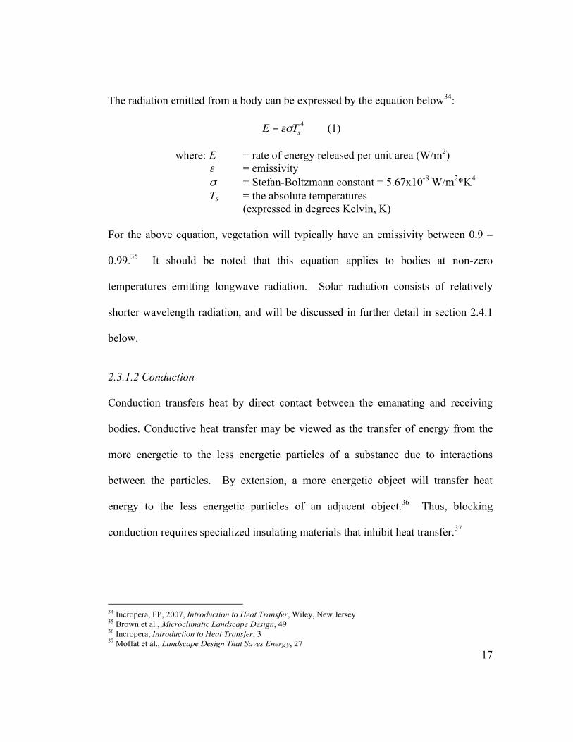
The radiation emitted from a body can be expressed by the equation below34:
E = Ts4 (1)
where: E = rate of energy released per unit area (W/m2)
= emissivity
= Stefan-Boltzmann constant = 5.67x10⁻⁸ W/m2*K4
Ts = the absolute temperatures (expressed in degrees Kelvin, K)
For the above equation, vegetation will typically have an emissivity between 0.9 –
0.99.35 It should be noted that this equation applies to bodies at non-zero
temperatures emitting longwave radiation. Solar radiation consists of relatively
shorter wavelength radiation, and will be discussed in further detail in section 2.4.1
below.
2.3.1.2 Conduction
Conduction transfers heat by direct contact between the emanating and receiving
bodies. Conductive heat transfer may be viewed as the transfer of energy from the
more energetic to the less energetic particles of a substance due to interactions
between the particles. By extension, a more energetic object will transfer heat
energy to the less energetic particles of an adjacent object.36 Thus, blocking
conduction requires specialized insulating materials that inhibit heat transfer.37
34 Incropera, FP, 2007, Introduction to Heat Transfer, Wiley, New Jersey 35 Brown et al., Microclimatic Landscape Design, 49 36 Incropera, Introduction to Heat Transfer, 3 37 Moffat et al., Landscape Design That Saves Energy, 27
18
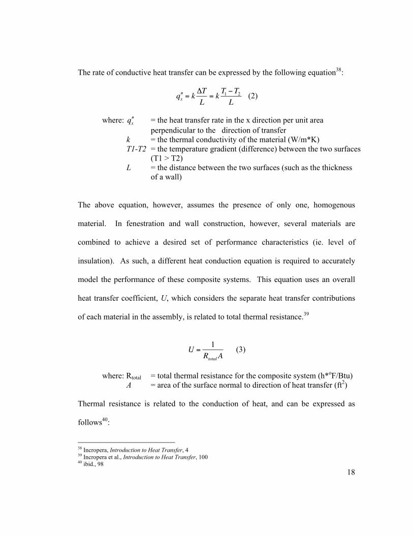
The rate of conductive heat transfer can be expressed by the following equation38:
q x = kT
L= k
T1 T2L
(2)
where: q x = the heat transfer rate in the x direction per unit area
perpendicular to the direction of transfer k = the thermal conductivity of the material (W/m*K) T1-T2 = the temperature gradient (difference) between the two surfaces
(T1 > T2) L = the distance between the two surfaces (such as the thickness
of a wall)
The above equation, however, assumes the presence of only one, homogenous
material. In fenestration and wall construction, however, several materials are
combined to achieve a desired set of performance characteristics (ie. level of
insulation). As such, a different heat conduction equation is required to accurately
model the performance of these composite systems. This equation uses an overall
heat transfer coefficient, U, which considers the separate heat transfer contributions
of each material in the assembly, is related to total thermal resistance.39
U =1
Rtotal A (3)
where: Rtotal = total thermal resistance for the composite system (h*oF/Btu) A = area of the surface normal to direction of heat transfer (ft2) Thermal resistance is related to the conduction of heat, and can be expressed as
follows40:
38 Incropera, Introduction to Heat Transfer, 4 39 Incropera et al., Introduction to Heat Transfer, 100 40 ibid., 98
19
R =L
kA (4)
where: L = thickness of the material k = thermal conductivity of the material
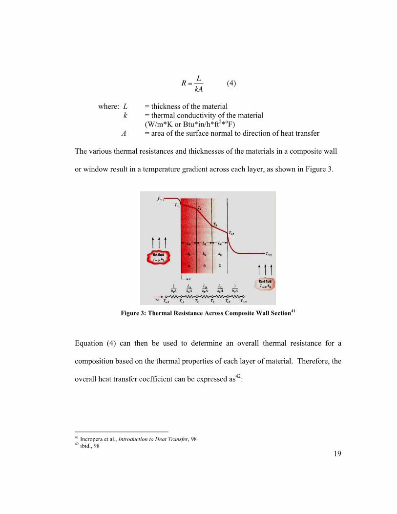
(W/m*K or Btu*in/h*ft2*oF) A = area of the surface normal to direction of heat transfer The various thermal resistances and thicknesses of the materials in a composite wall
or window result in a temperature gradient across each layer, as shown in Figure 3.
Figure 3: Thermal Resistance Across Composite Wall Section41
Equation (4) can then be used to determine an overall thermal resistance for a
composition based on the thermal properties of each layer of material. Therefore, the
overall heat transfer coefficient can be expressed as42:
41 Incropera et al., Introduction to Heat Transfer, 98 42 ibid., 98
20
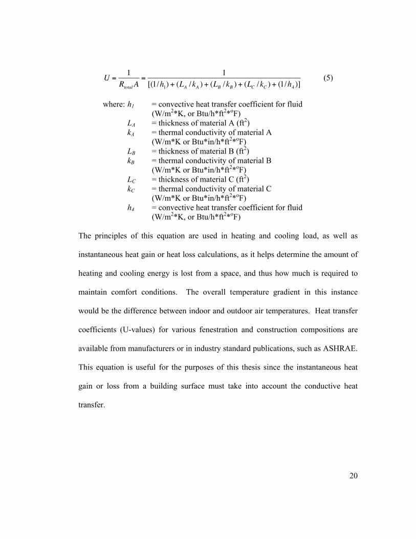
U =1
Rtotal A=
1
[(1/h1) + (LA /kA ) + (LB /kB ) + (LC /kC ) + (1/h4 )] (5)
where: h1 = convective heat transfer coefficient for fluid
(W/m2*K, or Btu/h*ft2*oF) LA = thickness of material A (ft2) kA = thermal conductivity of material A
(W/m*K or Btu*in/h*ft2*oF) LB = thickness of material B (ft2) kB = thermal conductivity of material B
(W/m*K or Btu*in/h*ft2*oF) LC = thickness of material C (ft2) kC = thermal conductivity of material C
(W/m*K or Btu*in/h*ft2*oF) h4 = convective heat transfer coefficient for fluid
(W/m2*K, or Btu/h*ft2*oF) The principles of this equation are used in heating and cooling load, as well as
instantaneous heat gain or heat loss calculations, as it helps determine the amount of
heating and cooling energy is lost from a space, and thus how much is required to
maintain comfort conditions. The overall temperature gradient in this instance
would be the difference between indoor and outdoor air temperatures. Heat transfer
coefficients (U-values) for various fenestration and construction compositions are
available from manufacturers or in industry standard publications, such as ASHRAE.
This equation is useful for the purposes of this thesis since the instantaneous heat
gain or loss from a building surface must take into account the conductive heat
transfer.
21
2.3.1.3 Convection
Convection conveys heat in a movable, fluid media, including air and water.43 The
heat transfer is comprised of two mechanisms: energy transfer due to random
molecular motion (diffusion), and energy transferred by the bulk, or macroscopic,
motion of the fluid.44 This motion, combined with the presence of a temperature
gradient, contributes to heat transfer.45 Convective heat transfer can be prevented by
the use of physical barriers to inhibit the movement of these fluids.46
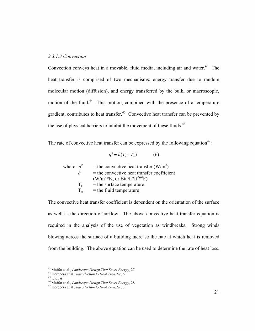
The rate of convective heat transfer can be expressed by the following equation47:
q = h(Ts T ) (6)
where: q = the convective heat transfer (W/m2)
h = the convective heat transfer coefficient (W/m2*K, or Btu/h*ft2*oF)
Ts = the surface temperature T = the fluid temperature
The convective heat transfer coefficient is dependent on the orientation of the surface
as well as the direction of airflow. The above convective heat transfer equation is
required in the analysis of the use of vegetation as windbreaks. Strong winds
blowing across the surface of a building increase the rate at which heat is removed
from the building. The above equation can be used to determine the rate of heat loss.
43 Moffat et al., Landscape Design That Saves Energy, 27 44 Incropera et al., Introduction to Heat Transfer, 6 45 ibid., 6 46 Moffat et al., Landscape Design That Saves Energy, 28 47 Incropera et al., Introduction to Heat Transfer, 8
22
As will be discussed in later sections, vegetation can be strategically placed adjacent
to a building to reduce the convective heat loss from the surface.
2.3.1.4 Change of State
The heat transferred (or stored) in a change of state is the heat required to melt a
substance from a solid to a liquid or conversely the heat required to evaporate a
liquid to a gas. This change of state is also known as latent heat transfer. Latent heat
transfer allows plants to evaporate large amounts of water by drawing heat from the
air, thus producing a cooling effect. This phenomenon, known as evapotranspiration,
enables vegetation to cool surrounding air temperature and is discussed in further
detail in Section 2.6. This is relevant since a reduction in surrounding air
temperature during the hot summer months can reduce conductive heat transfer from
building surfaces, thus reducing the amount of cooling required to maintain indoor
comfort conditions.
2.3.2 COOLING LOADS
Since the program for this thesis was developed for use in the hot, arid climate of
Los Angeles, energy transfer relating only to heat gain and increased cooling load
will be discussed. Several load calculation methods have been published in North
America. Two different methods of determining heat gain and thus cooling load are
discussed in further detail below.
23
2.3.2.1 Residential Design Cooling Loads
The American Society of Heating, Refrigerating, and Air-Conditioning Engineers
(ASHRAE) Fundamentals Handbook provides detailed methods for calculating
residential heating and cooling loads. The Handbook provides different approaches
for calculating residential and non-residential loads by acknowledging that unique
features for calculating loads and equipment sizes distinguish residential buildings
from other types.48 Several of these features are identified as follows49:
• Smaller internal heat gains – loads are primarily imposed by heat gain or loss
through structural components and by air leakage or ventilation
• Varied use of spaces – use of spaces is more flexible than in commercial
buildings
• Fewer zones – generally conditioned as single zone or, at most, a few zones
• Greater distribution losses – ducts are frequently installed in attics or other
unconditioned buffer spaces, resulting in significant leakage since ducts are
often insufficiently insulated
• Partial loads – loads are determined by outside conditions and since only a
few days of each season are design days, the units operate at partial load
during most of the season
48 American Society of Heating, Refrigerating, and Air-Conditioning Engineers, 2005, 2005 Fundamentals
Handbook, ASHRAE, Atlanta 49 ibid., 29.1
24
The 2005 Fundamentals Handbook provides an extensively revised method for
calculating cooling loads. Methods presented in earlier editions of the handbook
involved the use of a Cooling Load Temperature Difference/Cooling Load Factor
(CLTD/CLF) form; significantly simplified to facilitate manual calculations.50 The
method presented in the 2005 edition is the Residential Load Factor (RLF) method,
and is a simplified procedure derived from the more detailed Residential Heat
Balance (RHB) method.51
The Residential Heat Balance method is an extension of the Heat Balance (HB)
method, which allows for detailed simulation of space temperatures and heat flows
by considering a cooling load profile over a 24-hour period.52 The RLF method was
derived from several thousand RHB cooling load results for a range of climates and
building types.53 Statistical regression techniques were used to define values for the
load factors presented in the Handbook.54 These values were validated by comparing
RLF and RHB results for buildings that were not involved in the original regression
analysis.55
The above method of determining cooling loads is useful primarily for calculating
peak loads sizing cooling mechanical systems. The purposes of this thesis requires
50 ASHRAE, 2005 Fundamentals Handbook, 29.2 51 ibid., 29.2 52 ibid., 29.2 53 ibid., 29.2 54 ibid., 29.2 55 ibid., 29.2
25
an instantaneous method of calculating heat transfer since the intent is to quantify
reductions in energy transfer due to the presence of trees. An appropriate method is
presented as follows.
2.3.2.2 Instantaneous Cooling Load Calculations
The 2005 Fundamentals Handbook also provides instantaneous heat gain calculation
through fenestration surfaces. This equation is provided as follows:
Q =U Apf (Tout Tin ) + SHGC Apf Et (7)
where: Q = instantaneous energy flow (Btu/h) U = overall coefficient of heat transfer (Btu/h*ft2*oF) Tin = interior air temperature (oF) Tout = exterior air temperature (oF) Apf = total projected area of fenestration (ft2) SHGC = solar heat gain coefficient Et = incident total irradiance (Btu/h*ft2)
The above equation results in a heat gain value of Btu/h, with the instantaneous heat
gain through the window being a direct result of the solar radiation incident on the
fenestration surface. The value for Et is the sum total comprised of direct normal,
diffuse sky, and reflected radiation. The equation is given below:
Et = EDN cos + Ed + Er (8)
where: Et = incident total irradiance (Btu/h*ft2) = angle of incidence
EDN = direct normal radiation (Btu/h*ft2) Ed = diffuse sky radiation (Btu/h*ft2) Er = reflected radiation (Btu/h*ft2)
The value for direct normal radiation is corrected by the cosine of the angle of
incidence. The angle of incidence for any surface is defined as the angle between the
26
incoming solar rays and a line normal to that surface.56 It is related to the solar
altitude angle ( ), to the surface solar azimuth ( ), and to the tilt angle of the surface
from the horizontal ( ).57 Methods for calculated solar altitude and surface solar
azimuth will be discussed in Chapter 3, section 3.3.
The equation for determining the angle of incidence is:
cos = cos cos sin + sin cos (9)
where: = angle of incidence
= solar altitude angle
= surface solar azimuth angle
= tilt angle of the surface from the horizontal
For a vertical surface, such as a wall, the tilt angle of the surface is 90o. Thus
equation (9) is simplified and becomes:
cos V = cos cos (10)
Equations (7), (8) and (9) are used to determine the difference in instantaneous heat
gain from the presence of trees. When calculating the instantaneous heat gain with
the presence of trees, the projected area of fenestration is corrected to reflect the
percentage of window that is in shade from the tree. The direct normal and diffuse
sky radiation values are corrected based on the transmissivity of the tree at that time
56 ASHRAE, 2005 Fundamentals Handbook, 31.16 57 ibid., 31.16

27
of the year, which is based on the foliation present on the tree during that particular
season.
2.4 SHADING
The most widely acknowledged and experienced benefit of the presence of trees in a
landscape is the production of shade, which is accompanied by subsequent filtering
of solar radiation. The following sections discuss in further detail the physics of
solar radiation and the effect of plants on transmission and absorption of such
radiation.
2.4.1 SOLAR RADIATION
An understanding of the components and behaviour of solar radiation is necessary to
properly implement effective landscape design to reduce energy consumption.
Similarly, it is necessary to understand the movement of the sun as it travels an arc in
the sky before planning an energy-efficient design.58
Firstly, solar energy consists of a range of wavelengths, from very short ultraviolet
wavelengths to relatively longer infrared wavelengths.59 Most of the solar energy
can be categorized as either visible energy (which humans see and which plants use
58 Moffat et al., Landscape Design That Saves Energy, 31 59 ibid., 47
28
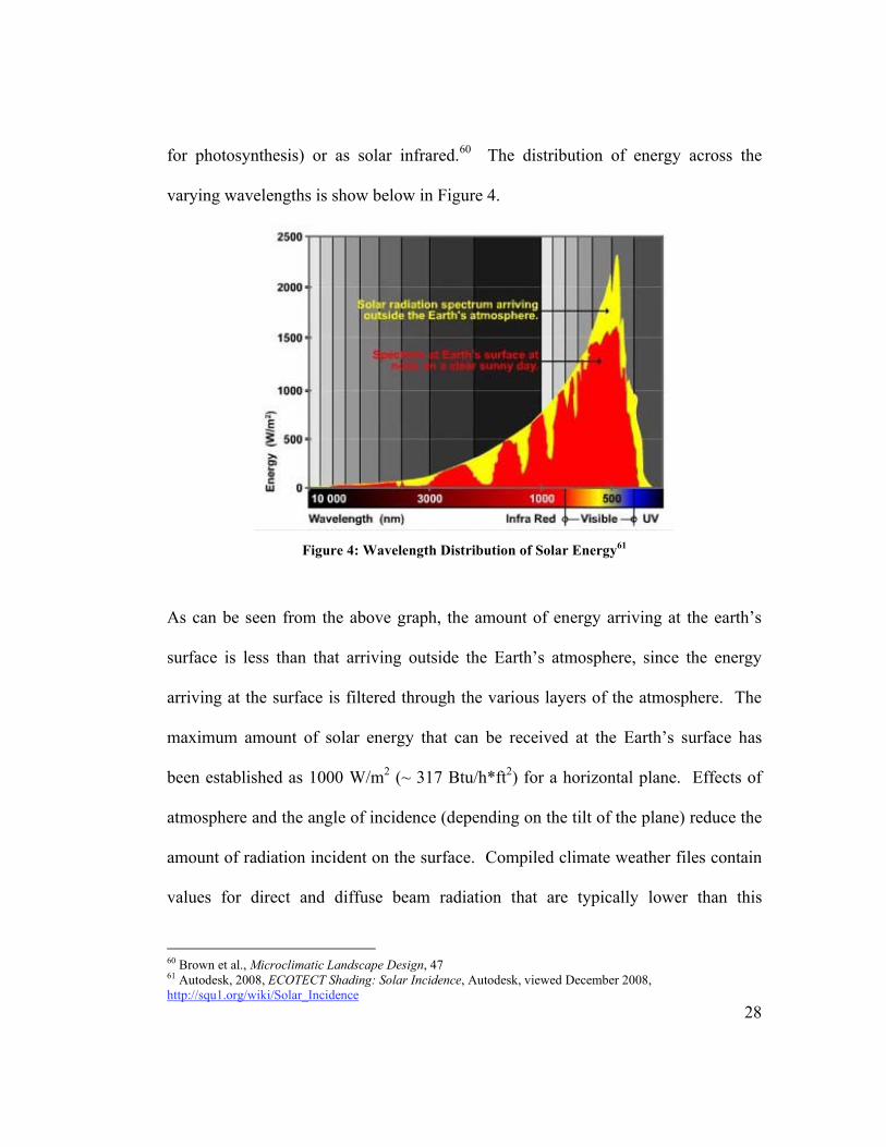
for photosynthesis) or as solar infrared.60 The distribution of energy across the
varying wavelengths is show below in Figure 4.
Figure 4: Wavelength Distribution of Solar Energy61
As can be seen from the above graph, the amount of energy arriving at the earth’s
surface is less than that arriving outside the Earth’s atmosphere, since the energy
arriving at the surface is filtered through the various layers of the atmosphere. The
maximum amount of solar energy that can be received at the Earth’s surface has
been established as 1000 W/m2 (~ 317 Btu/h*ft2) for a horizontal plane. Effects of
atmosphere and the angle of incidence (depending on the tilt of the plane) reduce the
amount of radiation incident on the surface. Compiled climate weather files contain
values for direct and diffuse beam radiation that are typically lower than this
60 Brown et al., Microclimatic Landscape Design, 47 61 Autodesk, 2008, ECOTECT Shading: Solar Incidence, Autodesk, viewed December 2008, http://squ1.org/wiki/Solar_Incidence

29
hypothetical maximum value since the measurements reflect the filtering effects of
atmosphere. The amount of radiation incident on the surface is also affected by the
angle of the sun as its path varies daily and throughout the seasons.
The solar path can be described by a set of two angles: the altitude angle (which is
the absolute height in the sky), and the bearing or azimuth angle (which is the
distance the sun travels on its path between the eastern sunrise and western sunset).62
The azimuth angle can be measured from either North or South. Conventions used
for this thesis are further discussed in Chapter 3. It is important to determine these
angles because the ability of the sun to add radiant heat to a building is dependent on
the sun’s position in the sky as well as on the intensity of sunlight.63 As mentioned
above, the intensity of radiant energy varies throughout the seasons as the sun angle
changes. At lower winter angles, the sun’s radiant heat must pass through a greater
portion of atmosphere, thus reducing it’s intensity.64
Incident radiation alone does not completely determine the amount of energy
absorbed by a surface. Material properties determine the amount of radiation
reflected, absorbed, and also transmitted by or through the surface.
62 Moffat et al., Landscape Design That Saves Energy, 31 63 ibid., 35 64 ibid., 35

30
2.4.2 TERRESTRIAL RADIATION
Terrestrial radiation occurs at wavelengths longer than those that comprise solar
energy. It can be described as the radiation that is emitted by all objects on the
earth’s surface, by clouds, and by the sky itself.65 The radiation emitted by these
objects is a function of their temperature and the surface emissivity (which is defined
as the ratio of energy radiated by the material to that radiated by a black body at the
same temperature). The energy temperature relationship is shown below.
Energy = S (T + 273)4 (11)
where: S = a constant, 5.67x10⁻⁸ (W/m2) T = temperature of the surface (oC)
Plants can affect both the solar and terrestrial radiation. This is discussed further in
the following section.
2.4.3 RADIATION AND PLANTS
The following section outlines how plants affect the various forms of radiation
outlined above.
2.4.3.1 Effect of Plants on Solar Radiation
Plants can have a significant impact on the solar radiation incident on a surface.
Plants absorb solar radiation and cast shade; and also use most of the captured
65 Brown et al., Microclimatic Landscape Design, 50
31
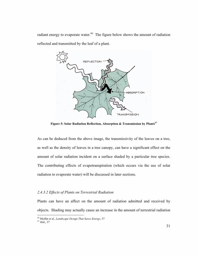
radiant energy to evaporate water.66 The figure below shows the amount of radiation
reflected and transmitted by the leaf of a plant.
Figure 5: Solar Radiation Reflection, Absorption & Transmission by Plants67
As can be deduced from the above image, the transmissivity of the leaves on a tree,
as well as the density of leaves in a tree canopy, can have a significant effect on the
amount of solar radiation incident on a surface shaded by a particular tree species.
The contributing effects of evapotranspiration (which occurs via the use of solar
radiation to evaporate water) will be discussed in later sections.
2.4.3.2 Effects of Plants on Terrestrial Radiation
Plants can have an affect on the amount of radiation admitted and received by
objects. Shading may actually cause an increase in the amount of terrestrial radiation
66 Moffat et al., Landscape Design That Saves Energy, 37 67 ibid., 37
32
received by an adjacent object since the sky emits a lower value of radiation than the
tree.68 This slight increase, however, is generally insignificant compared to the
reduction in solar radiation incident on the surface, especially since the tree
maintains lower surface temperatures by evapotranspiration.69 Plants also have the
ability to lower the surrounding ambient air temperature via evapotranspiration.
Lowering the ambient air temperature can also serve to lower surface temperatures
of nearby objects. Large numbers of trees, however, would be required for this
phenomenon to occur.
2.4.4 CALCULATING COOLING EFFECTS OF TREE SHADE
In order to determine the savings that be achieved from the shade provided by trees,
it is necessary to determine the shade pattern cast by the tree(s), and also to compute
the shaded and unshaded areas on a wall surface. Several methods for shading
computation have been developed.
A particular study developed a shading design software tool in MATLAB that can
perform shading calculations for any type of window system at a specific time and
place.70 The concepts used to develop this tool were expanded on in a 2006 article
outlining a modified algorithm to perform shading calculations.71 The authors define
68 Brown et al., Microclimatic Landscape Design, 54 69 ibid., 54 70 Chirarattananon, S & Rajapakse, A, A New Tool for Designing External Sun Shading Devices, Asiant Institute of Technology, viewed December 2008, http://www.energy-based.nrct.go.th/Article/Ts-3%20new%20tool%20for%20designing%20external%20sun%20shading%20devices.pdf 71 Pongpattana, C & Rakkwamsuk, P, 2006, ‘Efficient Algorithm and Computing Tool for Shading Calculation’, Songklanakarin Journal of Science and Technology, vol. 28, no. 2, March – April, pp 375-386
33
a plane with a tilt angle, , and azimuth, . The position of the sun is also defined by
solar altitude, , and solar azimuth, ; both of which are dependent on time, date and
latitude of the plane being considered.
Another study also incorporated the method of defining plane orientation and
analysis based on solar coordinates, but subsequently used a scanline algorithm to
perform a shading analysis.72 The building wall plane in question is rotated via
matrix transformations using solar angles to determine if the plane is in line with the
sun. If so, the program proceeds to determine the percentage shading from a tree on
the building surface using a scanline algorithm. Total radiation incident on the
surface is calculated by modelling the building surface and tree shadow as a set of
overlapping polygons. The scanline algorithm analyzes shading polygon by
scanning across the window polygon in slices, and determining the area of shade for
each slice (if there is any). These shade slices are added to generate an overall
shaded area for the window. The scanline algorithm will be discussed in further
detail in the following chapters.
2.4.5 PREVIOUS STUDIES
Several studies have been published that used computer simulations to investigate
the effects of tree shade on building energy use. These studies concluded that shade
72 Schiler, M, 1979, ‘Foliage Effects on Computer Simulation of Building Energy Load Calculations’, Master’s Thesis, Columbia, New York
34
from a single, well-placed, mature tree (about 25 ft crown diameter) could reduce
annual air-conditioning use by 2 – 8% (40 – 300 kWh) and peak cooling demand by
2 – 10% (0.15 – 0.5 kW) for various cities across the United States.73 Conversely, it
is also acknowledged, however, that trees placed for summer sun shading can also
have the adverse effect of reducing solar access in winter, thus potentially increasing
energy used for space heating.74 Several computer simulations found that shade
from trees positioned at various distances from a building’s south side often
increased annual building energy use for space heating.75
A study conducted by James Simpson and Gregory McPherson explored the
potential of tree shade for reducing residential energy use in several climate zones
throughout California.76 The study considered yard trees at a variety of orientations
around the building, as well as the effects of building energy efficiency. Shade
patterns projected onto the building from various tree configurations were calculated
using the Shadow Pattern Simulator (SPS) program. These results were then used in
an energy use simulation program known as MICROPAS to predict the effects of
tree shade on space conditioning.77 The base case structure used in the study was a
single story frame house, built to California Title 24 standards (R-19 wall insulation,
R-38 ceiling insulation, double-pane windows, gas furnace efficiency of 78%, and an
73 McPherson, EG & Simpson, JR, 1996, ‘Potential of Tree Shade for Reducing Residential Energy Use in California’, Journal of Aboriculture, vol. 22, no. 1, pp 10-18 74 ibid., 11 75 ibid., 11 76 ibid., 11 77 ibid., 11
35
air conditioner seasonal energy efficiency ratio of 10).78 Finally, energy use was
simulated in California climate zones 2, 4, 11, 12, and 13.
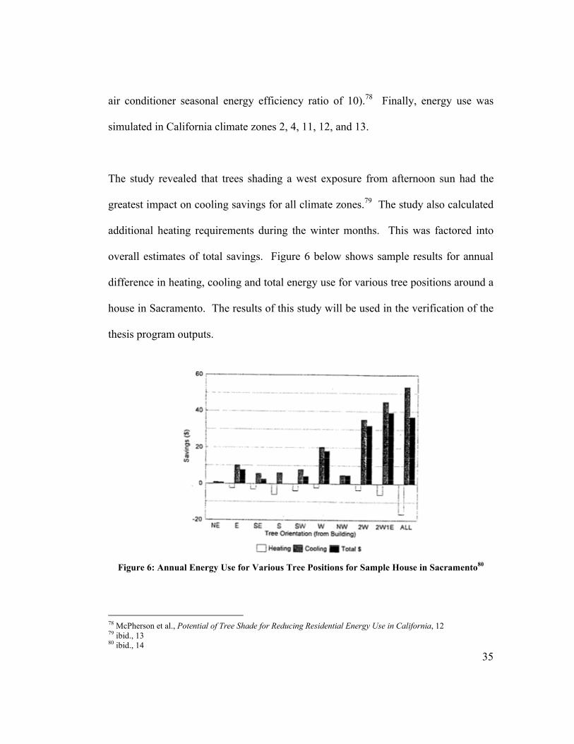
The study revealed that trees shading a west exposure from afternoon sun had the
greatest impact on cooling savings for all climate zones.79 The study also calculated
additional heating requirements during the winter months. This was factored into
overall estimates of total savings. Figure 6 below shows sample results for annual
difference in heating, cooling and total energy use for various tree positions around a
house in Sacramento. The results of this study will be used in the verification of the
thesis program outputs.
Figure 6: Annual Energy Use for Various Tree Positions for Sample House in Sacramento80
78 McPherson et al., Potential of Tree Shade for Reducing Residential Energy Use in California, 12 79 ibid., 13 80 ibid., 14
36
It can be seen from this graph that the greatest savings for single trees were achieved
by placing the tree to the West and East of the house. Greater savings were achieved
by placing two trees to the west, and even more by placing two trees to the west and
one to the east.
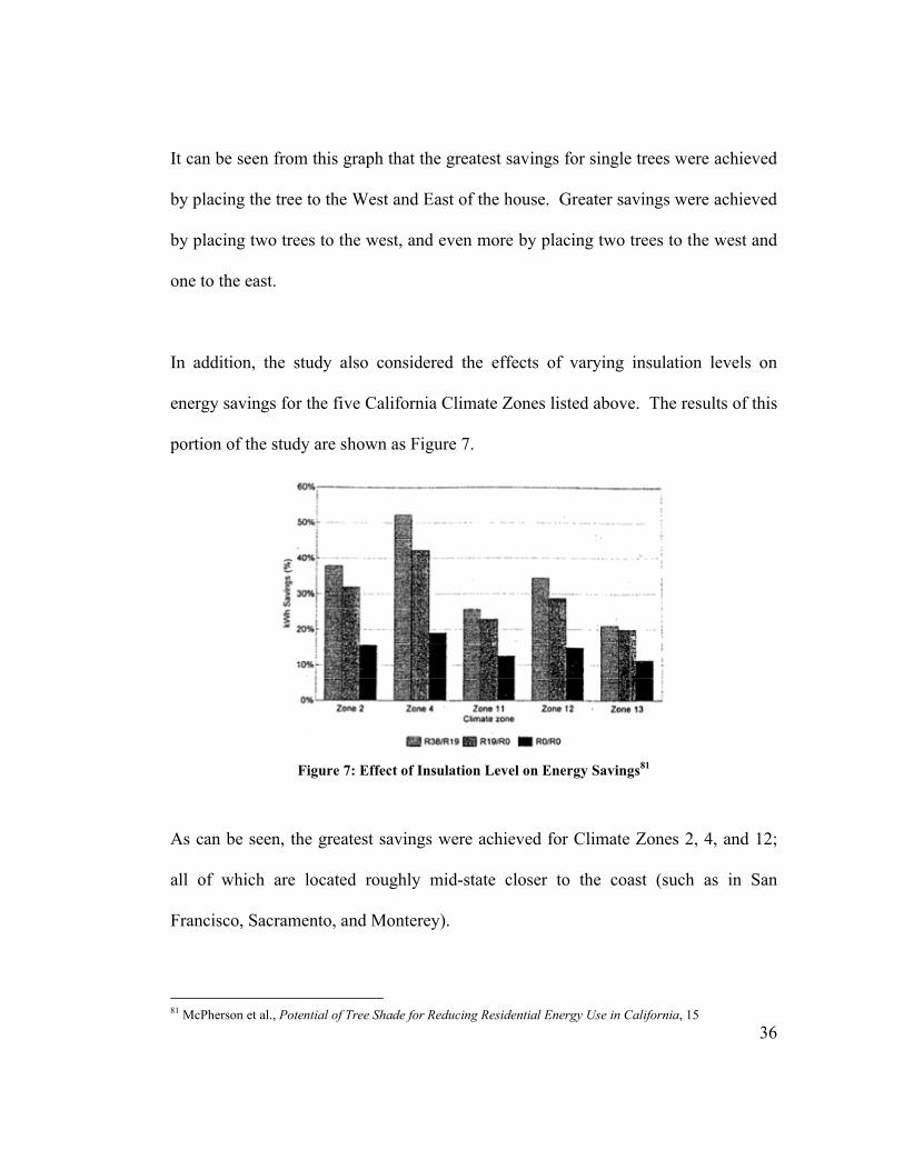
In addition, the study also considered the effects of varying insulation levels on
energy savings for the five California Climate Zones listed above. The results of this
portion of the study are shown as Figure 7.
Figure 7: Effect of Insulation Level on Energy Savings81
As can be seen, the greatest savings were achieved for Climate Zones 2, 4, and 12;
all of which are located roughly mid-state closer to the coast (such as in San
Francisco, Sacramento, and Monterey).
81 McPherson et al., Potential of Tree Shade for Reducing Residential Energy Use in California, 15
37
2.5 WIND BREAKS
Trees can also generate savings during the heating months by acting as wind breaks
that block cold winter winds. The following section discusses the effects of plants
on wind and their corresponding use as windbreaks.
2.5.1 WIND
In addition to supplying radiation to the earth’s surface, the sun also provides the
energy that drives atmospheric systems.82 At the macro-scale, differences in
temperature between the earth’s poles and the equator result in large masses of cold
and warm air that continually mix along an interface, known as a weather front.83 At
the regional level, weather maps can be drawn and tracked along such weather fronts
by creating isobars (lines of equal barometric readings) that delineate areas of high
and low pressure.84 The interaction of these pressure zones creates air movement
from the areas of higher pressure to areas of lower pressure, which, in turn, produces
wind. In general, the above process of mixing air masses of different temperatures
and pressures is what produces the winds that are experienced in a particular
location.
82 Moffat, AS & Schiler, M, 1993, Energy-Efficient and Environmental Landscaping, Appropriate Solutions Press, South Newfane, Vermont 83 Brown et al., Microclimatic Landscape Design, 31 84 ibid., 32

38
2.5.1.1 Wind Patterns
A certain location will be accompanied by characteristic prevailing wind patterns,
which describes the intensity and amount of time wind is experienced at different
directions. Although it is not possible to accurately predict the exact time, duration,
and speed of wind, measurements can be made and general patterns can be observed.
These patterns can be annual or daily and can be illustrated as prevailing winds on
special diagrams known as wind roses. These are graphical representations that
display the percentage of time the wind is blowing from each direction.85 Figure 8
below shows an annual wind rose for Los Angeles. This wind rose was created
using Weather Tool, and Los Angeles weather data available in .WEA file format.
85 Brown et al., Microclimatic Landscape Design, 126
39
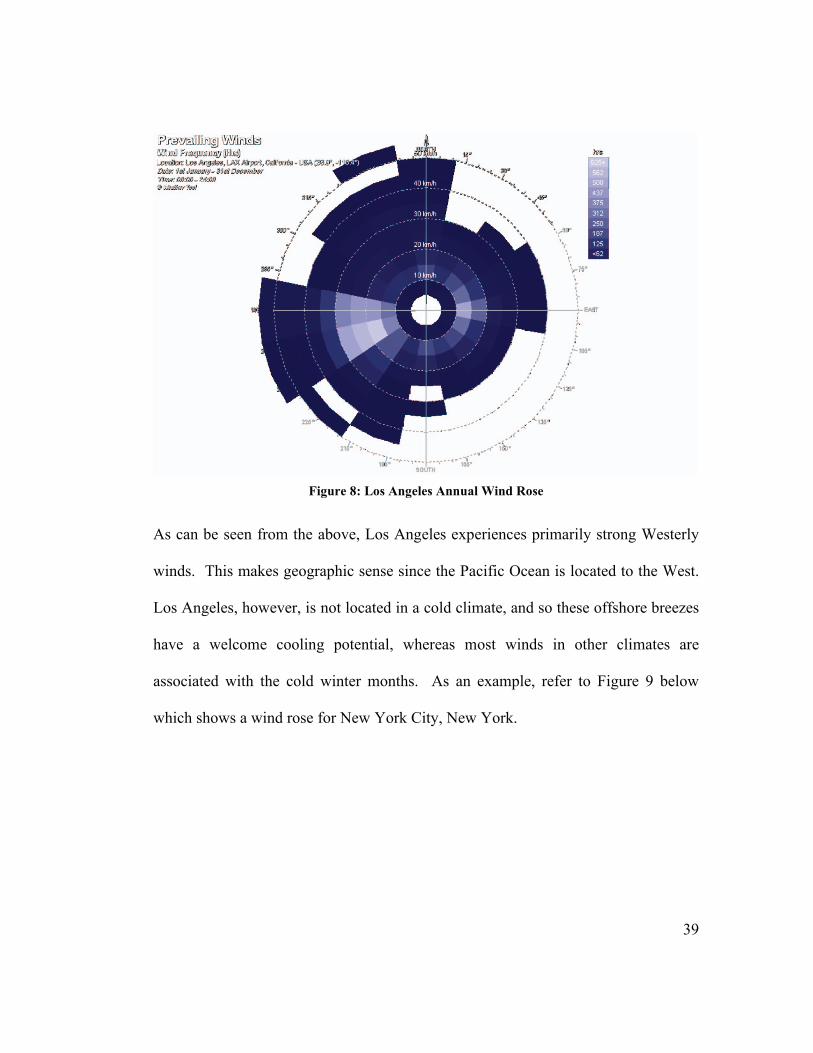
Figure 8: Los Angeles Annual Wind Rose
As can be seen from the above, Los Angeles experiences primarily strong Westerly
winds. This makes geographic sense since the Pacific Ocean is located to the West.
Los Angeles, however, is not located in a cold climate, and so these offshore breezes
have a welcome cooling potential, whereas most winds in other climates are
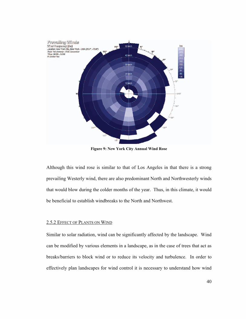
associated with the cold winter months. As an example, refer to Figure 9 below
which shows a wind rose for New York City, New York.
40
Figure 9: New York City Annual Wind Rose
Although this wind rose is similar to that of Los Angeles in that there is a strong
prevailing Westerly wind, there are also predominant North and Northwesterly winds
that would blow during the colder months of the year. Thus, in this climate, it would
be beneficial to establish windbreaks to the North and Northwest.
2.5.2 EFFECT OF PLANTS ON WIND
Similar to solar radiation, wind can be significantly affected by the landscape. Wind
can be modified by various elements in a landscape, as in the case of trees that act as
breaks/barriers to block wind or to reduce its velocity and turbulence. In order to
effectively plan landscapes for wind control it is necessary to understand how wind
41
moves through a microclimate, to analyze the prevailing wind patterns (as discussed
above), and to understand the effect various landscape elements will have on the
behaviour of the wind.
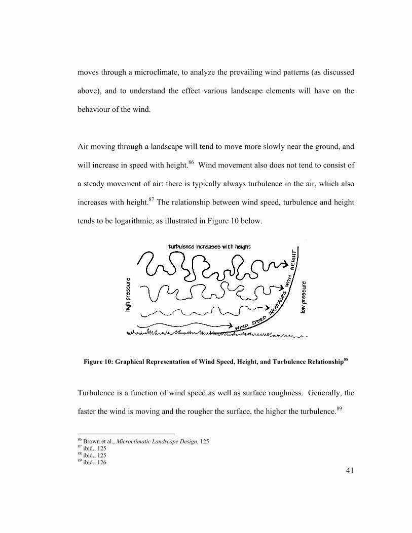
Air moving through a landscape will tend to move more slowly near the ground, and
will increase in speed with height.86 Wind movement also does not tend to consist of
a steady movement of air: there is typically always turbulence in the air, which also
increases with height.87 The relationship between wind speed, turbulence and height
tends to be logarithmic, as illustrated in Figure 10 below.
Figure 10: Graphical Representation of Wind Speed, Height, and Turbulence Relationship88
Turbulence is a function of wind speed as well as surface roughness. Generally, the
faster the wind is moving and the rougher the surface, the higher the turbulence.89
86 Brown et al., Microclimatic Landscape Design, 125 87 ibid., 125 88 ibid., 125 89 ibid., 126

42
The introduction of objects into the landscape will affect wind speed. Some objects
reduce and/or redirect wind speed, and others can actually increase it. An object
introduced into the landscape causes air to flow up, over and around its edges. When
air encounters such an object, a piling-up of molecules occurs on the upwind side.90
This back pressure creates a bubble of air next to the object that has a lower wind
speed than that in a freely flowing stream of air.91 Where the air is forced to go
around the edges of the object, the molecules speed up and this is experienced as an
increase in wind speed. Conversely, downwind of the windbreak there are fewer
molecules moving past at any given time. This is thus experienced as lower
windspeed relative to the free air stream as well as to the flow around the ends and
over the top of the object.92
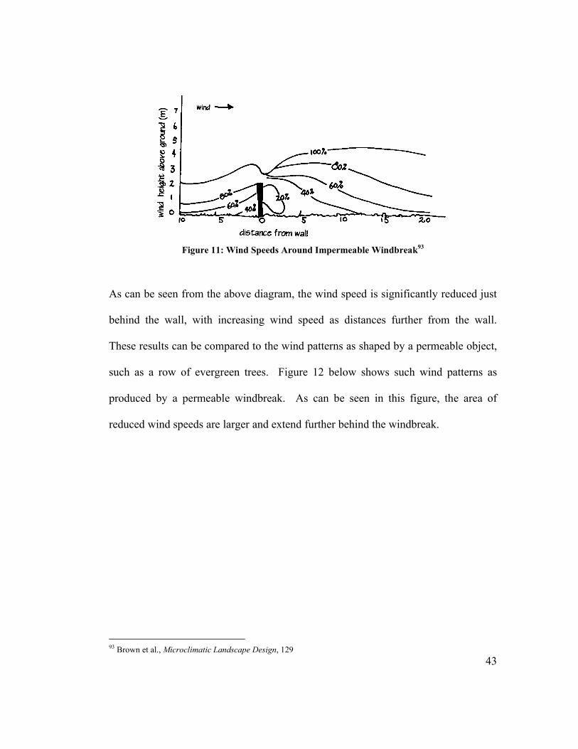
The area and pattern of reduced wind speeds is affected by the porosity of the object
or windbreak. Figure 11 below shows the affect of a solid object, such as a wall, on
the speed of wind moving through the landscape. The speeds shown in this diagram
are relative to a free stream of air moving at 2 meters (about 6.5 feet) above the
ground.
90 Brown et al., Microclimatic Landscape Design, 128 91 ibid., 128 92 ibid., 129
43
Figure 11: Wind Speeds Around Impermeable Windbreak93
As can be seen from the above diagram, the wind speed is significantly reduced just
behind the wall, with increasing wind speed as distances further from the wall.
These results can be compared to the wind patterns as shaped by a permeable object,
such as a row of evergreen trees. Figure 12 below shows such wind patterns as
produced by a permeable windbreak. As can be seen in this figure, the area of
reduced wind speeds are larger and extend further behind the windbreak.
93 Brown et al., Microclimatic Landscape Design, 129
44
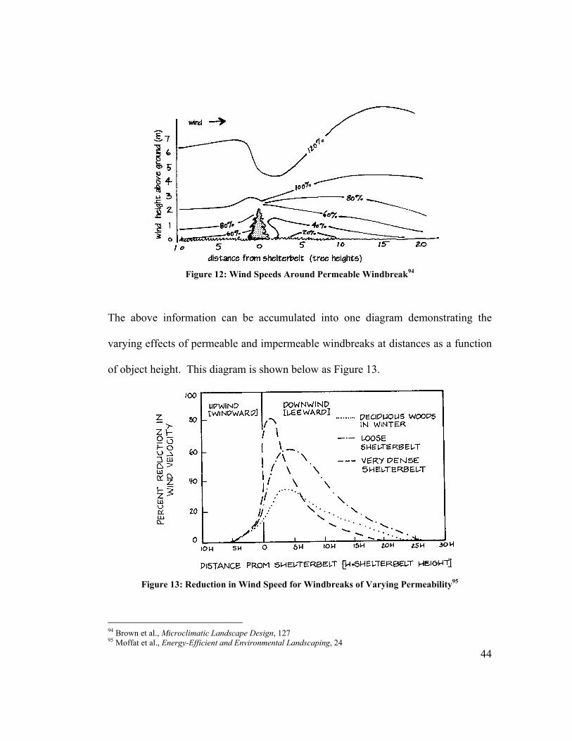
Figure 12: Wind Speeds Around Permeable Windbreak94
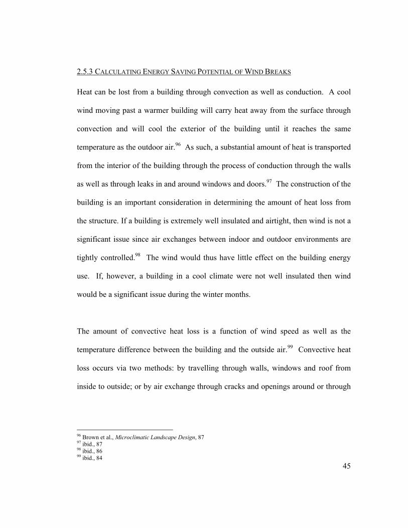
The above information can be accumulated into one diagram demonstrating the
varying effects of permeable and impermeable windbreaks at distances as a function
of object height. This diagram is shown below as Figure 13.
Figure 13: Reduction in Wind Speed for Windbreaks of Varying Permeability95
94 Brown et al., Microclimatic Landscape Design, 127 95 Moffat et al., Energy-Efficient and Environmental Landscaping, 24
45
2.5.3 CALCULATING ENERGY SAVING POTENTIAL OF WIND BREAKS
Heat can be lost from a building through convection as well as conduction. A cool
wind moving past a warmer building will carry heat away from the surface through
convection and will cool the exterior of the building until it reaches the same
temperature as the outdoor air.96 As such, a substantial amount of heat is transported
from the interior of the building through the process of conduction through the walls
as well as through leaks in and around windows and doors.97 The construction of the
building is an important consideration in determining the amount of heat loss from
the structure. If a building is extremely well insulated and airtight, then wind is not a
significant issue since air exchanges between indoor and outdoor environments are
tightly controlled.98 The wind would thus have little effect on the building energy
use. If, however, a building in a cool climate were not well insulated then wind
would be a significant issue during the winter months.
The amount of convective heat loss is a function of wind speed as well as the
temperature difference between the building and the outside air.99 Convective heat
loss occurs via two methods: by travelling through walls, windows and roof from
inside to outside; or by air exchange through cracks and openings around or through
96 Brown et al., Microclimatic Landscape Design, 87 97 ibid., 87 98 ibid., 86 99 ibid., 84
46
windows and doors.100 The most important factor in the amount of heat loss is the
speed of the wind striking the building. Generally, the higher the wind speed, the
greater the resulting heat loss.101 Conversely, it is possible to design landscape for
the purpose of channelling “cooling” winds into a building space during hot summer
months. The condition of a wind temperature being lower than the building
temperature during warm months, however, is limited in most regions, and so plants
are more typically used as wind breaks during the colder months.
Calculating the effects of reduced wind speed on the energy consumption of the
building involves estimating wind speeds at various heights and calculating the
corresponding convective heat loss from the surface. The generic equation that can
be used to calculate wind speeds up to 10 meters (about 33 feet) in height from the
ground is as follows:
W (z) =U10 {[ln(z
zos)]/(ln10
zow)} (12)
where: W(z) = Wind speed at a height z above the ground z = Height above the ground of the wind U10 = Wind speed at 10 m above the weather station zos = Constant based on height of vegetation at test site (zos = 0.13 x height of vegetation) zow = 0.13 x height of vegetation at weather station
The corresponding heat loss can be calculated using the equations for conduction and
convective heat loss as outlined above. Lowering the wind speed will reduce the
100 Brown et al., Microclimatic Landscape Design, 84 101 ibid., 84
47
convective heat loss at the surface of the building, thus narrowing the temperature
difference between indoor and outdoor wall temperatures, which, in turn, reduced
heat loss via conduction through walls.
2.5.3 PREVIOUS STUDIES
Several studies have also been published that estimate the effects of trees on wind
speed as well as the effect windbreaks on building energy consumption. One study
concluded that trees scattered throughout a neighbourhood can reduce wind speeds
by as much as 50%.102 Another study simulated the effect on heating energy use
from reduced infiltration as a result of the use of trees as a windshield. This study
found that three trees placed adjacent to the building reduced annual heating energy
consumption by 16%.103 In addition, other computer simulation studies confirmed
that windbreaks could reduce annual heating costs by 10 – 30%.104
A study by Greg McPherson was conducted to analyze the affects of shading,
evapotranspirative cooling, and windbreaks on brick and wood-frame residential
buildings in Chicago of one-, two-, and three-story height.105 The computer
simulation software of Micropas 4.01 was used in the wind analysis for this study.
The outputs from the simulations were referenced with respect to actual building
data from buildings in Chicago to ensure that the realistic results were being
102 McPherson, EG, 1994, Energy Saving Potential of Trees in Chicago, USDA Forest Service General Technical Report NE-186, Davis, California 103 McPherson, Energy-Saving Potential of Trees in Chicago, 96 104 ibid., 96 105 ibid., 96
48
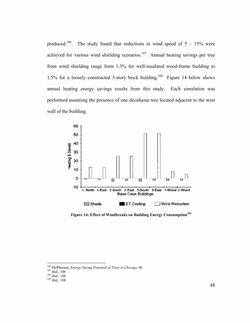
produced.106. The study found that reductions in wind speed of 5 – 15% were
achieved for various wind shielding scenarios.107 Annual heating savings per tree
from wind shielding range from 1.3% for well-insulated wood-frame building to
1.5% for a loosely constructed 3-story brick building.108 Figure 14 below shows
annual heating energy savings results from this study. Each simulation was
performed assuming the presence of one deciduous tree located adjacent to the west
wall of the building.
Figure 14: Effect of Windbreaks on Building Energy Consumption109
106 McPherson, Energy-Saving Potential of Trees in Chicago, 96 107 ibid., 106 108 ibid., 106 109 ibid., 108
49
2.6 EVAPOTRANSPIRATION
In addition to filtering solar radiation and diverting strong winds, trees also have the
capability to cool the surrounding air temperature. Trees have the ability to affect
the temperature of their microclimate through evaporation and transpiration of
moisture through leaves, a phenomenon known as evapotranspiration.110
Several studies have been conducted to determine, either through simulation or
measurement, the effects of evapotranspirative cooling on the surrounding
microclimate. Evapotranspiration (ET) can be defined as the loss of water to the
atmosphere by the combined process of evaporation (from soil and plant surfaces)
and transpiration (from plant tissues).111 Transpiration results from the vaporisation
of water within plant tissues and its loss through the stomata.112 Evaporation is the
conversion of water from liquid to vapour.113 The cooling effect is accomplished
through the release of moisture into the air, with subsequent evaporation of this
moisture due to hot air temperatures. The process is known as evaporative cooling.
Trees facilitate evaporative cooling by releasing moisture into the atmosphere
through the stomata of leaves (see Figure 15 below). As hot air passes over the
110 Akbari, H, Huang, YJ, Rosenfeld, AH & Taha, H, 1987, ‘The Potential of Vegetation in Reducing Summer Cooling Loads in Residential Buildings’, Journal of Climate and Applied Meteorology, vol. 26, September, pp 1103-1116 111 California Irrigation Management Information System, 2008, ET Overview, State of California, viewed November 2008, http://www.cimis.water.ca.gov/cimis/infoEtoOverview.jsp 112 Queensland Government Department of Employment, Economic Development and Innovation, 2008, Using
Evapotranspiration to Estimate Water Use, Queensland Government, viewed November 2008, http://www.dpi.qld.gov.au/cps/rde/dpi/hs.xsl/26_9829_ENA_HTML.htm 113 ibid., 1
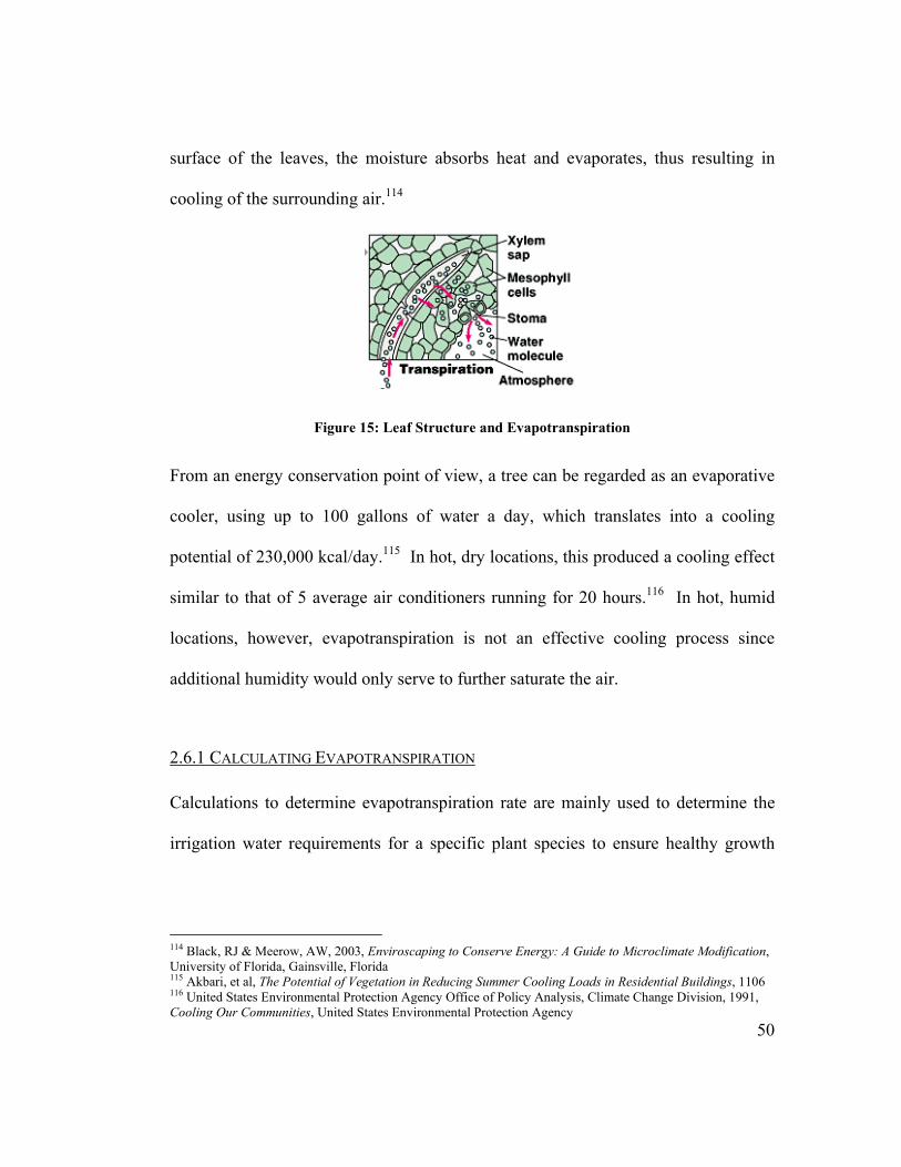
50
surface of the leaves, the moisture absorbs heat and evaporates, thus resulting in
cooling of the surrounding air.114
Figure 15: Leaf Structure and Evapotranspiration
From an energy conservation point of view, a tree can be regarded as an evaporative
cooler, using up to 100 gallons of water a day, which translates into a cooling
potential of 230,000 kcal/day.115 In hot, dry locations, this produced a cooling effect
similar to that of 5 average air conditioners running for 20 hours.116 In hot, humid
locations, however, evapotranspiration is not an effective cooling process since
additional humidity would only serve to further saturate the air.
2.6.1 CALCULATING EVAPOTRANSPIRATION
Calculations to determine evapotranspiration rate are mainly used to determine the
irrigation water requirements for a specific plant species to ensure healthy growth
114 Black, RJ & Meerow, AW, 2003, Enviroscaping to Conserve Energy: A Guide to Microclimate Modification, University of Florida, Gainsville, Florida 115 Akbari, et al, The Potential of Vegetation in Reducing Summer Cooling Loads in Residential Buildings, 1106 116 United States Environmental Protection Agency Office of Policy Analysis, Climate Change Division, 1991, Cooling Our Communities, United States Environmental Protection Agency

51
and productivity.117 Several equations are available, with their use depending on the
degree of accuracy necessary.
Evapotranspiration for a particular crop or species of tree (ETc) is determined by
multiplying a crop coefficient (Kc) by the reference evapotranspiration (ETo).118 The
reference evapotranspiration was developed as an indication of the evaporative
demand of the atmosphere independent of crop type and management: the only
factors affecting ETo are climatic parameters.119 The crop coefficient is a
dimensionless number, used in conjunction with ETo to estimate specific crop
evapotranspiration rates.120 It is representative of the fraction of water lost from the
crop relative to the reference evapotranspiration.121 The California Irrigation
Management Information System (CIMIS) has identified reference
evapotranspiration zones as well as reference evapotranspiration rates for selected
cities in California. The Food and Agriculture Organization (FAO) of the United
Nations and CIMIS both provide detailed tables of crop coefficients for various
agricultural crops.
117 California Irrigation Management Information System, ET Overview, 1 118 Saxena, M, 2002, Microclimate Modification: Calculating the Effects of Trees on Air Temperature, Heschong Mahone Group, Fair Oaks, California 119 United Nations Food and Agriculture Organization, 1998, Crop Evapotranspiration: Guidelines for
Computing Crop Water Requirements, Food and Agriculture Organization, viewed November 2008, http://www.fao.org/docrep/X0490E/X0490E00.htm 120 California Irrigation Management Information System, ET Overview, 1 121 California Department of Water Resources, A Guide to Estimating Irrigation Water Needs of Landscape
Planting in California, California Department of Water Resources, viewed November 2008, http://www.owue.water.ca.gov/docs/wucols00.pdf
52
The equation for calculating evapotranspiration based on crop coefficient and
reference evapotranspiration rate is thus as follows:
ETc = Kc ETo (13)
There are several methods available for calculating the reference evapotranspiration,
several of which are discussed below.
2.6.1.1 Penman-Monteith Equation
The FAO recommends the Penman-Monteith method as the standard method for
calculating reference evapotranspiration (ETo).122 It is recommended since it
presents a high likelihood of correctly predicting ETo in a wide range of locations
and climates.123 This method combines energy balance with mass transfer to form an
equation that computes the evaporation from an open water surface from standard
climatological records of sunshine, temperature, humidity, and wind speed.124 This
method was further revised to include aerodynamic and surface resistance factors.125
The resultant Penman-Monteith equation is shown below.
ETo =
(Rn G) + Ktime acp(es ea )
ra
+ 1+rsra
/ (14)
122 United Nations Food and Agriculture Organization, Crop Evapotranspiration, http://www.fao.org/docrep/X0490E/X0490E00.htm 123 ibid., http://www.fao.org/docrep/X0490E/X0490E00.htm 124 ibid., http://www.fao.org/docrep/X0490E/X0490E00.htm 125 ibid., http://www.fao.org/docrep/X0490E/X0490E00.htm
53
where: ETo = reference evapotranspiration (mm/d or mm/h) Rn = net radiation (MJ/m2d or MJ/m2h) G = soil heat flux (MJ/m2d or MJ/m2h) (es-ea) = vapour pressure deficit of the air (kPa) es = saturation vapour pressure of the air (kPa) ea = actual vapour pressure of the air (kPa) a = mean air density at constant air pressure (kg/m3)
cp = specific heat of the air (kPa/oC) = slope of saturation vapour press. temp relationship (kPa/oC)
= Psychrometric constant (kPa/oC)
rs = (bulk) surface resistance (s/m) ra = aerodynamic resistance (s/m) = latent heat of vaporization (MJ/kg)
Ktime = units conversion (86,400 s/d for ET in mm/d and equals 3600 s/h in mm/d)
A simplified alternative to the Penman-Monteith equation can be used to determine
the reference evapotranspiration when weather data are missing or are not available.
2.6.1.2 Hargreaves Equation
Unlike the full Penman-Monteith equation discussed above, the simplified
Hargreaves equation requires only daily maximum and minimum temperature
data.126 This equation is given as:
ETo = 0.0023(Tmean +17.8)(Tmax Tmin )0.5Ra (15)
where: ETo = reference evapotranspiration (mm/day or mm/h) Tmean = average of daily max and min temperatures (oC) Tmax = daily maximum temperature (oC) Tmin = daily minimum temperature (oC) Ra = extraterrestrial radiation (mm/day)
126 United Nations Food and Agriculture Organization, Crop Evapotranspiration, http://www.fao.org/docrep/X0490E/X0490E00.htm
54
2.6.2 PREVIOUS STUDIES
As mentioned previously, several studies have been conducted to determine the
effects of evapotranspirative cooling on the surrounding microclimate. In general,
the impact of one or several trees on ambient air temperatures and cooling loads are
small, though still relevant, compared to the shading effect.127 Several studies have
reported evapotranspirative cooling effects of up to 5oC (9oF), however this outcome
will mostly likely only result from large numbers of trees and expansive green
spaces.128 Even if large temperature drops are not achieved by small numbers of
trees, the advection of cool air can still lower the demand for air conditioning. This
has been exemplified in studies conducted in suburban areas. Such studies reported
smaller variations in daytime peaks of 2oC – 3oC (3.5oF – 5.5oF) between
neighbourhoods under mature tree canopies and newer areas with no trees.129 The
studies outlined below used computer simulations to determine the
evapotranspirative cooling potential of trees.
A study conducted by Huang et al. estimated the cooling effects of three trees around
a residential home using the DOE-2.1C building energy simulation program.130 The
study considered the combined and individual effects of reduced solar gain, reduced
wind speed, and evapotranspiration. The study sought to determine the amount of
127 McPherson, EG, 1994, Cooling Urban Heat Islands with Sustainable Landscapes, United States Center for Urban Forest Research, viewed October 2008, http://www.fs.fed.us/psw/programs/cufr/products/cufr_82_EM94_59.PDF 128 ibid., http://www.fs.fed.us/psw/programs/cufr/products/cufr_82_EM94_59.PDF, 159 129 Saxena, Microclimate Modification: Calculating the Effect of Trees on Air Temperature, 1 130 Akbari et al, The Potential of Vegetation in Reducing Summer Cooling Loads in Residential Buildings, 1106
55
evapotranspiration as a function of time and ambient conditions and then to relate the
amount of added moisture to changes in the microclimate.131 The study included
several U.S cities, and was based on a prototype house modelled as a single-story,
detached, wood frame structure built to standard U.S building practices (circa
1979).132 The results demonstrated an evapotranspirative cooling effect that
accounted for 70% of the annual energy savings and 68% of the peak savings.133
This study used a model for calculating evapotranspiration based on four types of
agricultural crops and on measurements of the ratio of evapotranspiration to solar
radiation.134 The authors admit that use of this model should be taken with caution,
as it had yet to be determined whether it was applicable for all climates and plant
types.135
A more recent study has expanded on this original work by Huang et al., and
incorporates the FAO recommended standard Penman-Monteith equation for
calculating evapotranspiration. This study identifies other limitations of the original
study, such as assuming little variation in temperature and humidity with air mixing
height, assuming uniform increase in cooling effect with increased number of trees,
and assuming that sufficient water will be available to trees (which is not always the
131 Akbari et al, The Potential of Vegetation in Reducing Summer Cooling Loads in Residential Buildings, 1106 132 ibid., 1110 133 McPherson, Cooling Urban Heat Islands with Sustainable Landscapes, 159 134 Akbari et al, The Potential of Vegetation in Reducing Summer Cooling Loads in Residential Buildings, 1107 135 ibid., 1108
56
case).136 The study thus seeks to incorporate the use of a dispersion pattern model in
conjunction with wind direction to quantify cooling from the moisture released from
trees.137 The study modelled several different scenarios, from a single home with
varying numbers of trees, to entire neighbourhood configurations. Three-
dimensional moisture contour plots were created around each home. These were
then used to determine the decrease in dry bulb temperature based on the increase in
humidity of the surrounding air. The study found that the dry bulb temperature could
decrease by as much as 1.37 degrees Fahrenheit around a single house with multiple
trees.138 Although important, the effects of this change in temperature would not be
as significant compared to reductions in energy use from the filtering of radiant heat
gain from tree shade.
Finally, a study produced by the United States Environmental Protection Agency
considered the effects of additional tree cover on three cities in hot, arid locations:
Sacramento, Lake Charles (LA), and Phoenix. The publication reported that direct
effects of shading accounted for only 10 – 35% of total energy savings, with the
remaining savings resulting from temperatures lowered by evapotranspiration.139
The following graph summarizes the findings of two different tree cover scenarios
for a typical, well-insulated, new house (shading effected are presented as direct,
while effects from evapotranspiration are shown as indirect).
136 Saxena, Microclimate Modification: Calculating the Effect of Trees on Air Temperature, 2 137 ibid., 2 138 ibid., 4 139 United States Environmental Protection Agency Office of Policy Analysis, Climate Change Division, Cooling
Our Communities, 34
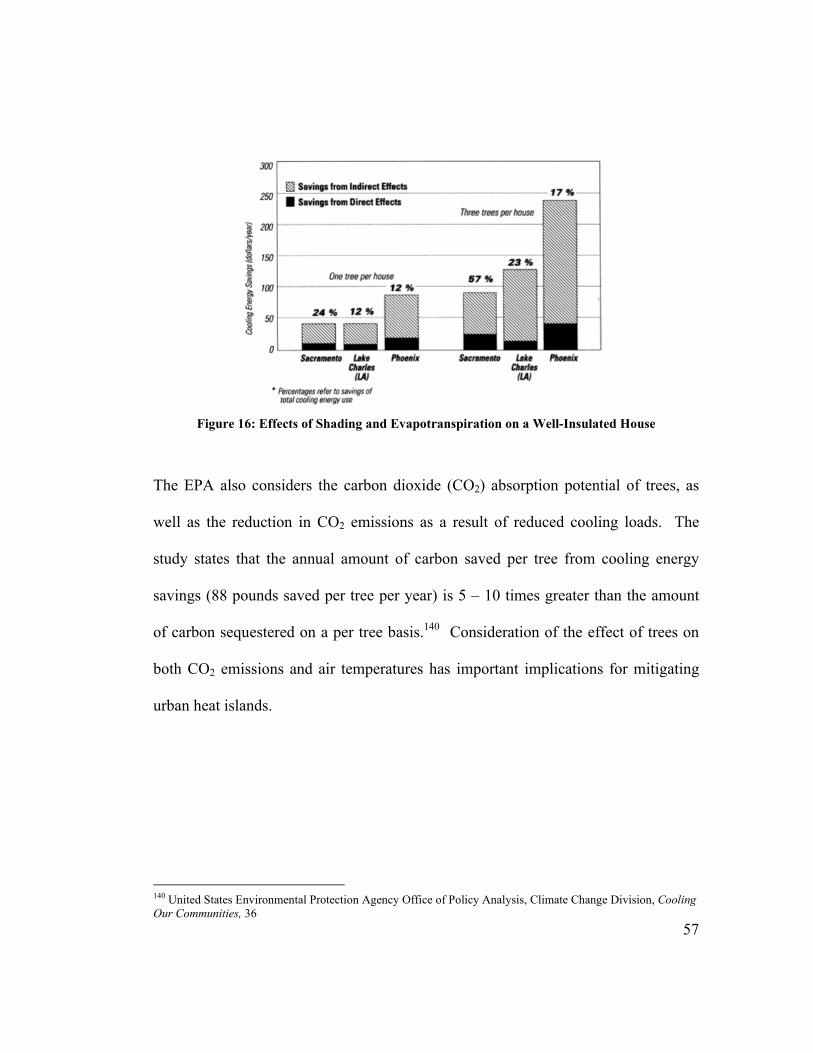
57
Figure 16: Effects of Shading and Evapotranspiration on a Well-Insulated House
The EPA also considers the carbon dioxide (CO2) absorption potential of trees, as
well as the reduction in CO2 emissions as a result of reduced cooling loads. The
study states that the annual amount of carbon saved per tree from cooling energy
savings (88 pounds saved per tree per year) is 5 – 10 times greater than the amount
of carbon sequestered on a per tree basis.140 Consideration of the effect of trees on
both CO2 emissions and air temperatures has important implications for mitigating
urban heat islands.
140 United States Environmental Protection Agency Office of Policy Analysis, Climate Change Division, Cooling
Our Communities, 36
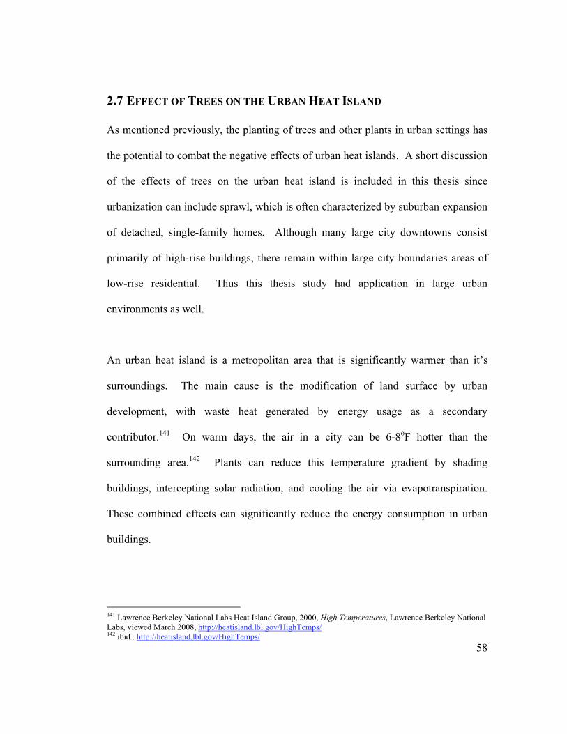
58
2.7 EFFECT OF TREES ON THE URBAN HEAT ISLAND
As mentioned previously, the planting of trees and other plants in urban settings has
the potential to combat the negative effects of urban heat islands. A short discussion
of the effects of trees on the urban heat island is included in this thesis since
urbanization can include sprawl, which is often characterized by suburban expansion
of detached, single-family homes. Although many large city downtowns consist
primarily of high-rise buildings, there remain within large city boundaries areas of
low-rise residential. Thus this thesis study had application in large urban
environments as well.
An urban heat island is a metropolitan area that is significantly warmer than it’s
surroundings. The main cause is the modification of land surface by urban
development, with waste heat generated by energy usage as a secondary
contributor.141 On warm days, the air in a city can be 6-8oF hotter than the
surrounding area.142 Plants can reduce this temperature gradient by shading
buildings, intercepting solar radiation, and cooling the air via evapotranspiration.
These combined effects can significantly reduce the energy consumption in urban
buildings.
141 Lawrence Berkeley National Labs Heat Island Group, 2000, High Temperatures, Lawrence Berkeley National Labs, viewed March 2008, http://heatisland.lbl.gov/HighTemps/ 142 ibid., http://heatisland.lbl.gov/HighTemps/
59
Higher temperatures in an urban heat island result in increased energy use due to
greater demand for air-conditioning. For example, during a warm afternoon in Los
Angeles, demand for electric power rises nearly 2% for every degree Fahrenheit the
daily max temperature rises.143 This trend is shown below in Figure 17. It is
estimated that about 1-1.5 gigawatts of power are used to compensate for the impact
of heat islands.144
Figure 17: Urban Temperature and Electricity Use Trend145
It is estimated that a full-size deciduous tree evaporates 100 gallons of water during a
sunny summer day, which uses up about 660,000 Btu of energy. This corresponds to
a cooling effect equivalent to 5 average (10,000 Btu) air-conditioners.146 In addition
to providing cooling and reducing energy consumption, trees in greater numbers
143 Lawrence Berkeley National Labs Heat Island Group, 2000, Energy Use, Lawrence Berkeley National Labs, viewed March 2008, http://heatisland.lbl.gov/EnergyUse/ 144 ibid., http://heatisland.lbl.gov/EnergyUse/ 145 ibid., http://heatisland.lbl.gov/EnergyUse/ 146 Moffat et al., Landscape Design That Saves Energy, 18
60
(known as urban forests) located throughout an urban setting can have other positive
effects, such as storm water run-off reduction, increasing air/water quality, as well as
providing carbon storage.
The Lawrence Berkeley Labs Heat Island Group conducted a study in Los Angeles
to determine the effects of adding green space (trees) and lightening surfaces. The
Group divided Los Angeles into hundreds of portions, estimated how much
vegetation and reflective surfaces could be added to each location, and then added
trees and lightened surfaces to 15% of possible areas.147 The results of the
simulation showed that summer temperatures at 3:00 pm dropped by 6oF, which
would cut the need for air-conditioning by 18%, or 1.04 billion kWh.148 The
increased cover could also lower the need for peak electrical generating capacity by
about 1,500 MW, which is equivalent to 2 or 3 large power plants.149 The results
were simplified to conclude that a single tree in Los Angeles could save an
additional 6.6 lbs of carbon per year by lowering the need for air-conditioning, plus
15 kg more if that same tree directly shades a building.150 If the entire community
dropped one degree in temperature (from trees and lighter surfaces), then each
building’s air conditioning load would go down – even those not directly shaded.151
147 Lawrence Berkeley National labs Heat Island Group, 1999, Estimating Energy Saving Potentials of Heat
Island Mitigation Measure, viewed March 2008, http://eetd.lbl.gov/HeatIsland/EnergyUse/Overview/ 148 ibid., http://eetd.lbl.gov/HeatIsland/EnergyUse/Overview/ 149 ibid., http://eetd.lbl.gov/HeatIsland/EnergyUse/Overview/ 150 ibid., http://eetd.lbl.gov/HeatIsland/EnergyUse/Overview/ 151 Lawrence Berkeley National labs Heat Island Group, 1999, Estimating Energy Saving Potentials of Heat
Island Mitigation Measure, viewed March 2008, http://eetd.lbl.gov/HeatIsland/EnergyUse/Overview/
61
Indirect annual savings would thus total an additional 12% (0.7 billion kWh, or $12
million).152
The above analysis demonstrates the substantial positive effects increased tree cover
can have on the economics and environmental quality of large urban settings. As
outlined, planting even single trees can have a significant effect. Thus it is important
to target low-rise residential building owners to take initiative and implement
energy-efficient landscaping practices by planting trees and other elements in
strategic locations.
2.8 ENERGY-EFFICIENT RESIDENTIAL LANDSCAPE – DESIGN
APPROACHES
The purpose of any energy efficient landscape design is to control solar radiation or
wind, or both at the same time. In general, it is desirable to block or filter excess
solar radiation during the summer (cooling) months, while allowing it to penetrate
into the building during the winter (heating) months. These strategies are designed
to control solar heat gain. Conversely, landscape can also be used as wind breaks to
reduce infiltration and convective heat loss during winter (heating) months in cold
climates. The following sections outline, in further detail, specific landscape
152 Lawrence Berkeley National labs Heat Island Group, 1999, Estimating Energy Saving Potentials of Heat
Island Mitigation Measure, viewed March 2008, http://eetd.lbl.gov/HeatIsland/EnergyUse/Overview/
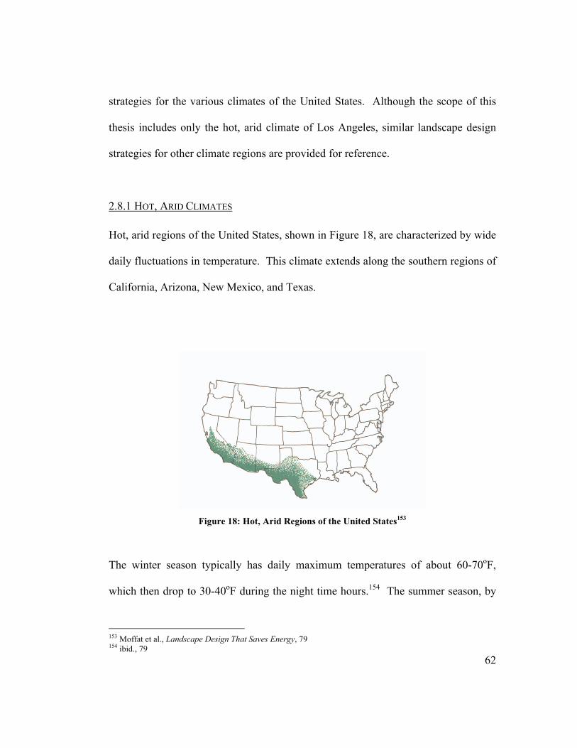
62
strategies for the various climates of the United States. Although the scope of this
thesis includes only the hot, arid climate of Los Angeles, similar landscape design
strategies for other climate regions are provided for reference.
2.8.1 HOT, ARID CLIMATES
Hot, arid regions of the United States, shown in Figure 18, are characterized by wide
daily fluctuations in temperature. This climate extends along the southern regions of
California, Arizona, New Mexico, and Texas.
Figure 18: Hot, Arid Regions of the United States153
The winter season typically has daily maximum temperatures of about 60-70oF,
which then drop to 30-40oF during the night time hours.154 The summer season, by
153 Moffat et al., Landscape Design That Saves Energy, 79 154 ibid., 79
63
comparison, is characterized by maximum temperatures above 100oF and minimum
temperatures between 70-80oF. These regions also experience hot seasonal winds,
which further contribute to the arid nature of the climate. Therefore, the goals of
energy efficient landscape are to temper and equalize extremes of temperature and
discourage hot winds while retaining any available moisture.155
2.8.1.1 Sun
Since hot, arid regions experience high daily temperatures year round, it is desirable
to control the amount of radiant energy reaching the building. The landscape should
be designed to block the incident solar radiation during the summer months when the
sun is traversing a high arc that is almost directly overhead during midday.156 This
can be accomplished by planting tall, high-crowned trees on the southern exposure
close to the home.157 In addition, sun can be controlled on the eastern side of the
building with low trees that have either light foliage or loose structure.158 These
types of trees are desirable because they will prevent excessive solar heat gain, but
will not completely block the morning sun. Finally, the sun must also be controlled
to the west, where afternoon heat gain can present a problem. Low trees with dense
foliage planted close to the home can prevent excessive heat build-up during this
time.159
155 Moffat et al., Landscape Design That Saves Energy, 79 156 ibid., 81 157 ibid., 81 158 ibid., 82 159 ibid., 83

64
2.8.1.2 Wind
Controlling wind for hot, arid regions is different from cooler regions since the
winds add additional heat rather than remove it. Similarly, though, blocking of these
winds can be accomplished through the use of windbreaks planted perpendicular to
the direction of prevailing winds.160
2.8.2 HOT, HUMID CLIMATES
The hot, humid regions of the United States are characterized by moisture-laden air
that prevents large fluctuations in daily temperature.161 These areas consist of
Florida, the coastal regions of Georgia, South Carolina, and the Gulf States (as
shown in Figure 19).
Figure 19: Hot, Humid Regions of the United States162
160 Moffat et al., Landscape Design that Saves Energy, 84 161 ibid., 95 162 ibid., 95
65
Hot, humid regions experience average temperatures between 65-85oF for over 75%
of the time, with sun shining on over 60% of all possible daylight hours.163 High
precipitation rates also contribute to the high levels of humidity. The goals of
landscape in these climates are thus to avoid heat storage and promote ventilation.164
Landscape can be used to reduce the retention of heat and humidity by shading
windows, walls, roofs, and air-conditioners, and by channelling cool breezes into
living areas.165
2.8.2.1 Sun
Similar to hot, arid climates, shading the building during the high, mid-summer
afternoon sun is the most important goal for energy-efficient landscape. The
southern façade should be shaded with high-crowned palms planted close to the
home.166 On the western side of the house, tall palm trees planted at some distance
from the house or shorter palms planted closer to the house will effectively shade
walls and windows from excessive afternoon solar heat gain.167
2.8.2.2 Wind
In hot, humid regions, cool winds that can dispel moisture and promote evaporation
should be channelled into the house via the use of a tree funnel.168 A funnel of trees
163 Moffat et al., Landscape Design that Saves Energy, 95 164 ibid., 96 165 ibid., 96 166 ibid., 99 167 ibid., 99 168 ibid., 102
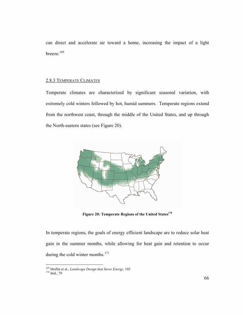
66
can direct and accelerate air toward a home, increasing the impact of a light
breeze.169
2.8.3 TEMPERATE CLIMATES
Temperate climates are characterized by significant seasonal variation, with
extremely cold winters followed by hot, humid summers. Temperate regions extend
from the northwest coast, through the middle of the United States, and up through
the North-eastern states (see Figure 20).
Figure 20: Temperate Regions of the United States170
In temperate regions, the goals of energy efficient landscape are to reduce solar heat
gain in the summer months, while allowing for heat gain and retention to occur
during the cold winter months.171
169 Moffat et al., Landscape Design that Saves Energy, 102 170 ibid., 79
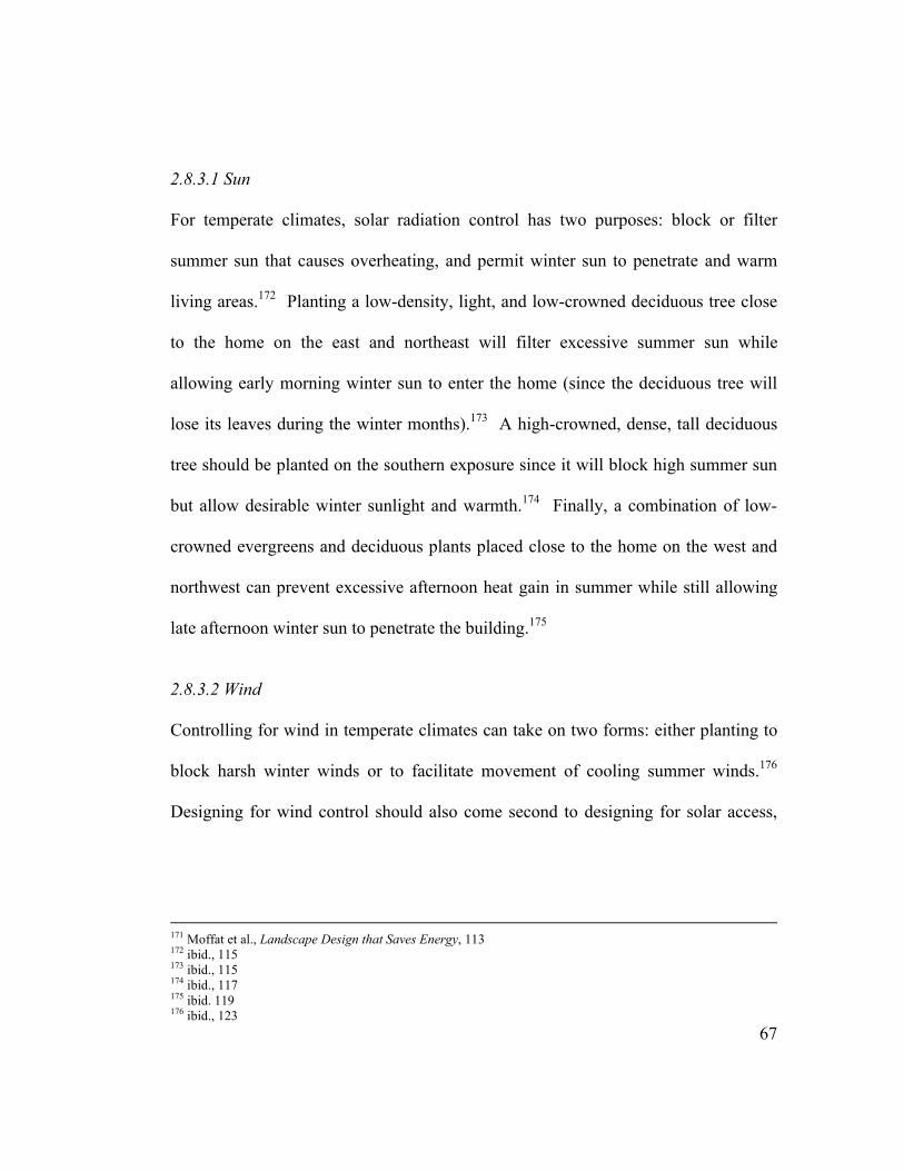
67
2.8.3.1 Sun
For temperate climates, solar radiation control has two purposes: block or filter
summer sun that causes overheating, and permit winter sun to penetrate and warm
living areas.172 Planting a low-density, light, and low-crowned deciduous tree close
to the home on the east and northeast will filter excessive summer sun while
allowing early morning winter sun to enter the home (since the deciduous tree will
lose its leaves during the winter months).173 A high-crowned, dense, tall deciduous
tree should be planted on the southern exposure since it will block high summer sun
but allow desirable winter sunlight and warmth.174 Finally, a combination of low-
crowned evergreens and deciduous plants placed close to the home on the west and
northwest can prevent excessive afternoon heat gain in summer while still allowing
late afternoon winter sun to penetrate the building.175
2.8.3.2 Wind
Controlling for wind in temperate climates can take on two forms: either planting to
block harsh winter winds or to facilitate movement of cooling summer winds.176
Designing for wind control should also come second to designing for solar access,
171 Moffat et al., Landscape Design that Saves Energy, 113 172 ibid., 115 173 ibid., 115 174 ibid., 117 175 ibid. 119 176 ibid., 123
68
since the latter generally has a greater effect on building energy use in these
climates.177
If the landscape is being designed to block winter winds that blow from the east or
west, planting tall trees with loose foliage two to five tree lengths away from the
house will block cold winds without filtering out all morning and evening solar
radiation.178 The same planting strategy can be used for prevailing southern winds;
however it is necessary to determine the maximum height of the trees based on
winter sun angles so as not to block the warming effect of the available winter sun.179
Alternatively, if designing to encourage cooling summer breezes, a funnel of tall
hedges can be used to direct prevailing winds toward the home.
2.8.4 COOL CLIMATES
Finally, the classification of a cool climate can be applied to the northern region of
the United States, including the North-central states along the Canadian border as
well as the northern areas of New England (see Figure 21 below).180
177 Moffat et al., Landscape Design That Saves Energy, 121 178 ibid., 122 179 ibid., 79 180 ibid., 63
69
Figure 21: Cool Climate Regions of the United States181
These regions are characterized by severe winters of extreme cold followed by
relatively cool summers.182 Average winter temperatures range from 0-20oF, while
summer temperatures reach an average maximum of 70-85oF.183 There is also
considerable variation in seasonal sunlight, with fourteen (14) hours of sunlight in
the summer and only eight (8) hours of sunlight during the winter months.184 The
region is also characterized by strong winter winds, which can greatly increase heat
loss. Given the above prevailing climatic conditions, it is apparent that landscape
design efforts should be directed at minimizing heating loads. This can be
accomplished by allowing winter sun (solar radiation) to penetrate the building while
simultaneously reducing the velocity of cold winds.
181 Moffat et al., Landscape Design that Saves Energy, 63 182 ibid., 63 183 ibid., 63 184 ibid., 63
70
2.8.4.1 Sun
As mentioned above, it is desirable to permit solar heat gain into the building during
the winter months. In midwinter, about 85% of the total solar energy is collected
between 9:00 am and 3:00 pm, when the sun travels a short, low arc from a bearing
angle of 150o (southeast) to 210o (southwest), reaching a noon altitude angle of only
20o.185 During the winter days, the warming impact of the sun is highest on vertical
south-facing wall surfaces and through vertical south-facing windows.186 As such,
the area around the building from southeast to southwest should be cleared of all
sun-blocking obstructions, including trees.
2.8.4.2 Wind
In addition to permitting winter sun access into the structure, solar heat gain should
also be complemented by implementing plant designs that deflect cold winds.
Strong cold winds cause increased heat loads through infiltration heat losses, as well
as convective heat loss from building surfaces. Rows of tall trees planted
perpendicular to the direction of the wind, and planted in stands that are wider than
the mature height of the trees, provide effective shields from cold winds.187
185 Moffat et al., Landscape Design that Saves Energy, 65 186 ibid., 65 187 ibid., 67
71
2.9 LANDSCAPE ELEMENTS
Various landscape elements exist for the modification of microclimates including
trees, shrubs, groundcovers, and water features. This thesis will focus on the
placement and selection of trees. Since the scope of the tool will be in the Southern
California region, the tree library database in the program will consist of native trees
to the region.
2.9.1 CALIFORNIA CLIMATE ZONES
The trees that grow in any region depend on the climate zone. Different plants are
suited for varying climates, thriving in some locations while potentially having
difficulty surviving in others. Section 2.8 above outlined planting strategies for 4
general climate zones in the United States. Although these climates provide general
descriptions of different regions of the United States, there are also several varying
climates within these broader zones.
There are different climate zone breakdowns currently available for the state of
California. One climate zone map has been developed by the California Energy
Commission, and comprises a breakdown of climate zones based on energy use,
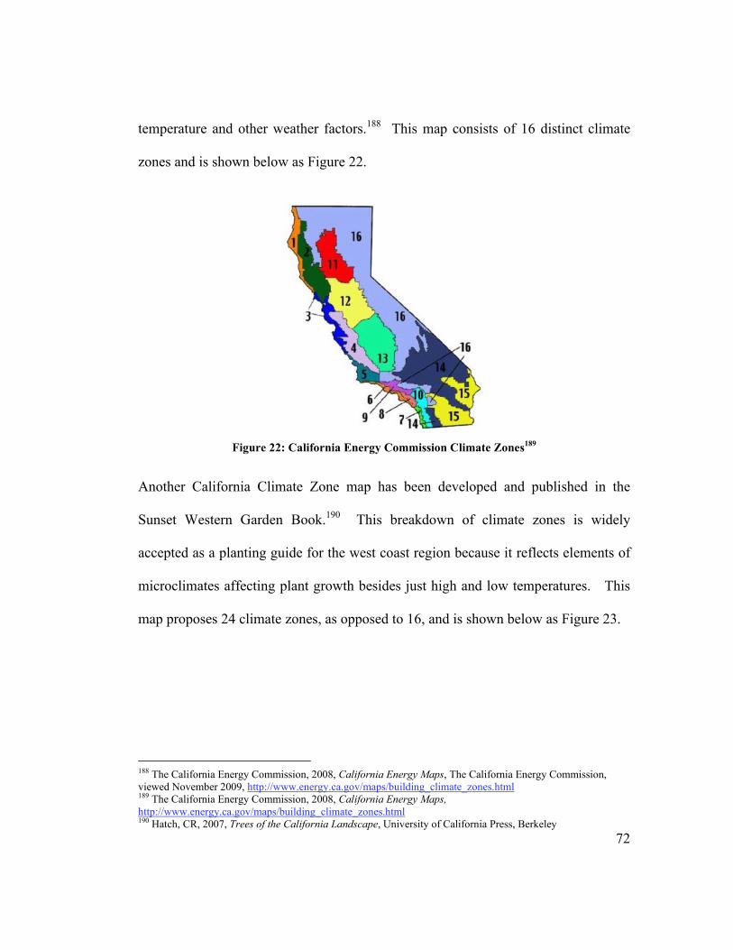
72
temperature and other weather factors.188 This map consists of 16 distinct climate
zones and is shown below as Figure 22.
Figure 22: California Energy Commission Climate Zones189
Another California Climate Zone map has been developed and published in the
Sunset Western Garden Book.190 This breakdown of climate zones is widely
accepted as a planting guide for the west coast region because it reflects elements of
microclimates affecting plant growth besides just high and low temperatures. This
map proposes 24 climate zones, as opposed to 16, and is shown below as Figure 23.
188 The California Energy Commission, 2008, California Energy Maps, The California Energy Commission, viewed November 2009, http://www.energy.ca.gov/maps/building_climate_zones.html 189 The California Energy Commission, 2008, California Energy Maps, http://www.energy.ca.gov/maps/building_climate_zones.html 190 Hatch, CR, 2007, Trees of the California Landscape, University of California Press, Berkeley
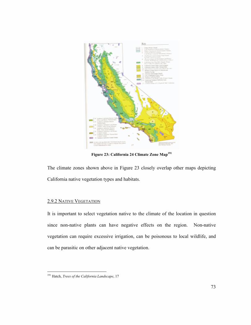
73
Figure 23: California 24 Climate Zone Map191
The climate zones shown above in Figure 23 closely overlap other maps depicting
California native vegetation types and habitats.
2.9.2 NATIVE VEGETATION
It is important to select vegetation native to the climate of the location in question
since non-native plants can have negative effects on the region. Non-native
vegetation can require excessive irrigation, can be poisonous to local wildlife, and
can be parasitic on other adjacent native vegetation.
191 Hatch, Trees of the California Landscape, 17
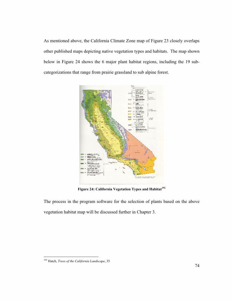
74
As mentioned above, the California Climate Zone map of Figure 23 closely overlaps
other published maps depicting native vegetation types and habitats. The map shown
below in Figure 24 shows the 6 major plant habitat regions, including the 19 sub-
categorizations that range from prairie grassland to sub alpine forest.
Figure 24: California Vegetation Types and Habitat192
The process in the program software for the selection of plants based on the above
vegetation habitat map will be discussed further in Chapter 3.
192 Hatch, Trees of the California Landscape, 35
75
CHAPTER 3 The following chapter outlines the theory and methods used in the program
development and calculations.
3.1 INSTANTANEOUS COOLING LOAD CALCULATION
Different methods for determining cooling loads were presented in Chapter 2. For
the purposes of this thesis, calculations based on first principles will be employed,
rather than the peak cooling load methods. Methods based on first principles will
provide instantaneous cooling loads that are required for building simulation
analyses. The main calculation is provided as Equations (7) and (8) in Chapter 2.
It should be noted that the instantaneous cooling load calculation for shaded surfaces
is also modified by the tree transmissivity. Since a tree canopy is not an opaque
surface, this value reflects the filtering effects of solar radiation by tree foliage (ie.
the amount of solar radiation being transmitted through the tree canopy). A lower
transmissivity value indicates a greater amount of filtering by the tree, and thus less
radiation being transmitted through the canopy to strike the shaded surface.
Conversely, a higher transmissivity indicates lower filtering by the tree, and thus a
greater amount of radiation is being transmitted through the canopy. The tree
transmissivity for deciduous trees typically changes depending on the time of year.
The transmissivity value of a tree canopy is lower in the summer when foliage is

76
denser, and so less radiation will penetrate through the leaves to strike a surface. The
transmissivity is higher in the winter when the tree loses much of its leaves and so
more solar radiation will penetrate through the tree canopy. The transmissivity value
is applied to the direct beam component in Equation (8).
Weather data is required to perform the instantaneous heat gain calculations. As
mentioned in Chapter 2, the study and documentation of a particular climate region
over a period of time allows for the development of a set of climate data. This data
is compiled from weather stations and is available for reference and/or download
from many sources. Climate data for use in this thesis will be downloaded from the
National Solar Radiation Data Base.193 This directory contains data files for the
typical meteorological year (TMY) data sets derived from 1961-1990 and 1991-2005
National Solar Radiation Data Base archives.194 The most recent TMY3 data sets
provide hourly values for temperature, solar radiation and other elements.195 The
TMY3 data files represent typical conditions and are intended for use in computer
simulations of building systems.196
193 National Solar Radiation Data Base, Typical Meteorological Year 3, United States Department of Energy Office of Energy Efficiency & Renewable Energy, viewed October 2008, http://rredc.nrel.gov/solar/old_data/nsrdb/1991-2005/tmy3/ 194 ibid., http://rredc.nrel.gov/solar/old_data/nsrdb/1991-2005/tmy3/ 195 ibid., http://rredc.nrel.gov/solar/old_data/nsrdb/1991-2005/tmy3/ 196 ibid., http://rredc.nrel.gov/solar/old_data/nsrdb/1991-2005/tmy3/
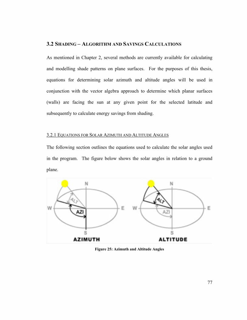
77
3.2 SHADING – ALGORITHM AND SAVINGS CALCULATIONS
As mentioned in Chapter 2, several methods are currently available for calculating
and modelling shade patterns on plane surfaces. For the purposes of this thesis,
equations for determining solar azimuth and altitude angles will be used in
conjunction with the vector algebra approach to determine which planar surfaces
(walls) are facing the sun at any given point for the selected latitude and
subsequently to calculate energy savings from shading.
3.2.1 EQUATIONS FOR SOLAR AZIMUTH AND ALTITUDE ANGLES
The following section outlines the equations used to calculate the solar angles used
in the program. The figure below shows the solar angles in relation to a ground
plane.
Figure 25: Azimuth and Altitude Angles
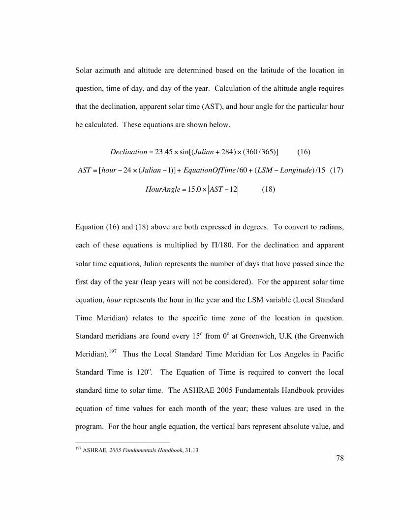
78
Solar azimuth and altitude are determined based on the latitude of the location in
question, time of day, and day of the year. Calculation of the altitude angle requires
that the declination, apparent solar time (AST), and hour angle for the particular hour
be calculated. These equations are shown below.
Declination = 23.45 sin[(Julian + 284) (360 /365)] (16)
AST = [hour 24 (Julian 1)]+ EquationOfTime /60 + (LSM Longitude) /15 (17)
HourAngle =15.0 AST 12 (18)
Equation (16) and (18) above are both expressed in degrees. To convert to radians,
each of these equations is multiplied by /180. For the declination and apparent
solar time equations, Julian represents the number of days that have passed since the
first day of the year (leap years will not be considered). For the apparent solar time
equation, hour represents the hour in the year and the LSM variable (Local Standard
Time Meridian) relates to the specific time zone of the location in question.
Standard meridians are found every 15o from 0o at Greenwich, U.K (the Greenwich
Meridian).197 Thus the Local Standard Time Meridian for Los Angeles in Pacific
Standard Time is 120o. The Equation of Time is required to convert the local
standard time to solar time. The ASHRAE 2005 Fundamentals Handbook provides
equation of time values for each month of the year; these values are used in the
program. For the hour angle equation, the vertical bars represent absolute value, and
197 ASHRAE, 2005 Fundamentals Handbook, 31.13

79
apparent solar time is expressed as a 24-hour clock (ie. 2:00 pm represented as
14:00). Based on the results of equations (16), (17) and (18) above, the sine of the
altitude can be calculated as follows:
sin(Altitude) = cos(Latitude)*cos(Declination)*cos(HourAngle) (19) + sin(Latitude)*sin(Declination)
In the above equation, latitude, declination, and hour angle must be expressed in
radians when converted to Visual Basic code. The altitude, in radians, is thus:
Altitude = asin(sin(Altitude)) (20)
Equation (20) is also expressed in radians. To convert to degrees, equation (20) is
multiplied by 180/ .
Finally, the equation for solar azimuth is as follows:
cos(Azimuth) =sin(Altitude) * sin(Latitude) sin(Declination)
cos(Altitude) *cos(Latitude) (21)
Similar to equation (19), latitude, declination, hour angle, and altitude must all be
expressed in radians.
3.2.2 DETERMINING PLANE FOR SHADING CALCULATION
The azimuth and altitude angles can be used to simplify the shading algorithm. Each
wall plane can be rotated and tilted so it is inline with the sun’s rays. This yields a
model and calculating problem in only 2-dimsensions as opposed to 3-dimensions.
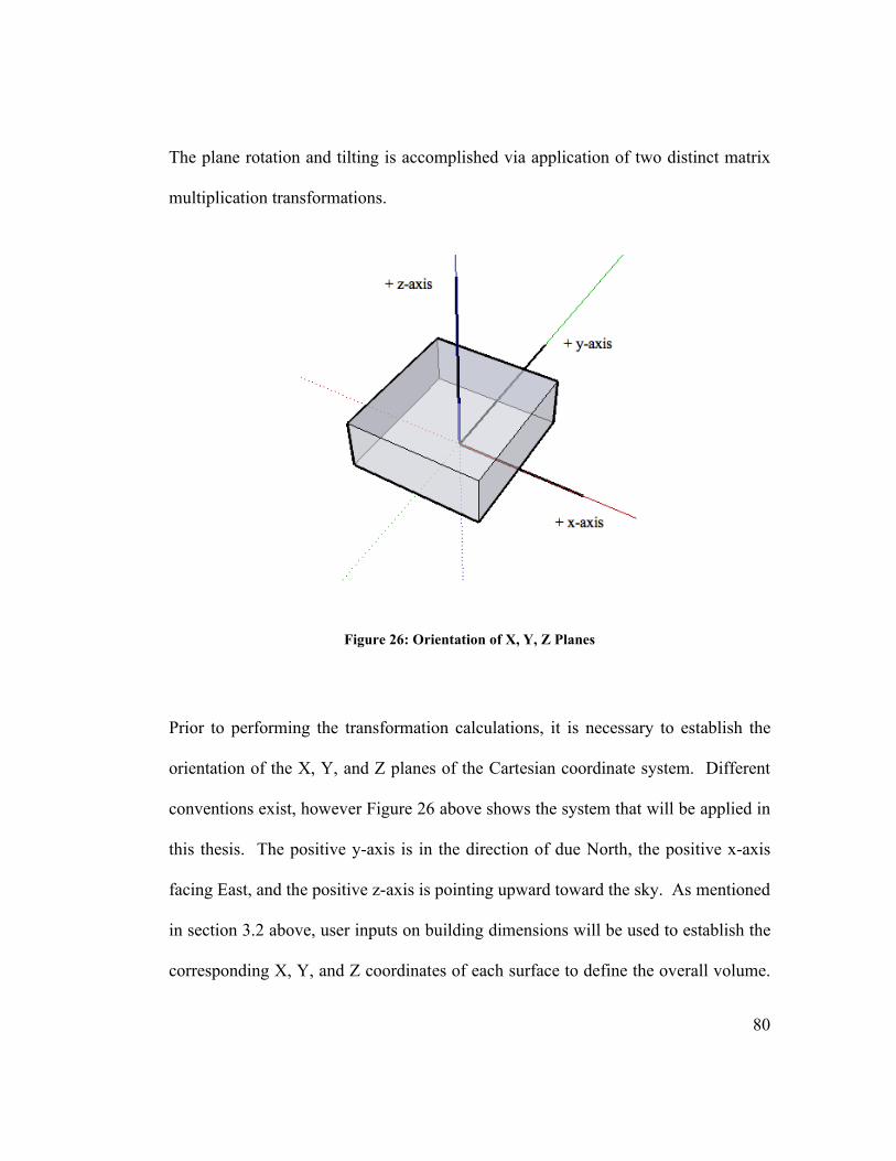
80
The plane rotation and tilting is accomplished via application of two distinct matrix
multiplication transformations.
Figure 26: Orientation of X, Y, Z Planes
Prior to performing the transformation calculations, it is necessary to establish the
orientation of the X, Y, and Z planes of the Cartesian coordinate system. Different
conventions exist, however Figure 26 above shows the system that will be applied in
this thesis. The positive y-axis is in the direction of due North, the positive x-axis
facing East, and the positive z-axis is pointing upward toward the sky. As mentioned
in section 3.2 above, user inputs on building dimensions will be used to establish the
corresponding X, Y, and Z coordinates of each surface to define the overall volume.
81
The building will be represented as a cubic/rectangular volume defined by a set of 8
distinct points, each having specific (x,y,z) coordinates. Each of these 8 points will
be transformed separately so as to transform the surface (plane) of each wall.
The wall to be examined is first rotated about the Z-axis (on the X-Y plane) via
application of a matrix transformation based on solar azimuth angle, and is then
tilted around the X-axis via application of a second matrix transformation involving
the solar altitude angle, so as to be perpendicular to the sun’s rays. Each rotation
assumes a point of reference around the origin (0,0,0). The matrix’s representing the
azimuth and altitude transformations are as follows:
Azimuth transformation:
M1[ ]x
y
=
x
y
where M1[ ] =
cos( ) sin( )
sin( ) cos( )
(22)
Altitude transformation:
M1[ ] y
z
=
y
z
where M2[ ] =
cos( ) sin( )
sin( ) cos( )
(23)
In the above equations, represents the solar azimuth angle, and represents the
solar altitude angle. The azimuth angle is assigned a positive or negative sign value
based on the time of day. After both the azimuth and altitude transformations have
been performed, each point will have a distinct set of coordinates describing their
82
final position for that hour. These coordinates will be [x’, y”, z’]. The same
transformations are performed for the points defining the window location, as well as
the points defining the tree polygon. These final points are used in the scanline
algorithm analysis.
Once the transformations have been completed, it is then necessary to determine
whether or not each respective plane is facing the sun. If the plane in question does
not face the sun, it can be discarded from the calculations for that given hour. It is
possible to ascertain this information through use of the surface solar azimuth, .
The ASHRAE Fundamentals Handbook outlines the surface solar azimuth as
follows:198
= (24)
where: = surface solar azimuth angle
= solar azimuth angle
= surface azimuth angle
The solar azimuth, , is positive for afternoon hours, and negative for morning
hours. Similarly, surfaces that face west have a positive surface azimuth angle, ;
and those facing east have a negative surface azimuth angle. For example, surfaces
facing directly east have a surface azimuth angle of -90o, surfaces facing south have
a surface azimuth angle of 0o, and surfaces facing west have a surface azimuth of
198 ASHRAE, 2005 Fundamentals Handbook, 31.15

83
90o.199 If the surface solar azimuth, , is greater than 90o or less than -90o, then the
surface is in the shade, and the wall surface is not facing the sun.
Since the sun’s position is constantly changing as it rotates about the house, it is
necessary to evaluate the surface solar azimuth for each wall plane at every hour for
the particular day between sunrise and sunset. Calculations are performed hourly
because the TMY3 weather data files contain hourly values. Thus calculations are
performed on an hourly basis to determine the instantaneous heat gain values, which
depend both on weather data and sun position.
3.2.3 PROJECTION OF SHADE PATTERN ONTO WALL PLANE
Once it has been established whether a particular wall plane is facing the sun (and
thus whether it is to be included in subsequent calculations), it is necessary to map
the projection of the shadow created by the tree onto the wall in order to determine if
the windows are shaded or unshaded. The method used in this thesis involves the
use of a scanline algorithm, as described in Chapter 2. The use of this algorithm in
the program will be discussed in further detail in Chapter 4.
3.2.4 CALCULATING SAVINGS FROM SHADING
The savings that are achieved from the presence of shade on a building surface can
be calculated by comparing the instantaneous heat gain through an unshaded surface
199 ASHRAE, 2005 Fundamentals Handbook, 31.16

84
versus the instantaneous heat gain through a shaded surface. As outlined in Chapter
2, instantaneous heat gain calculations consider the area of the surface in question as
well as the U-value of the fenestration construction assembly. For the purposes of
this thesis, only solar radiation in the form of direct beam and diffuse sky will be
taken into consideration when performing the heat gain calculations; terrestrial
radiation (radiation emitted by surrounding bodies) will not be included in the
analysis.
As mentioned in section 3.3.3 above, a scanline algorithm will be used to determine
the percentage of shadow falling on the fenestration surface for each hour in the
analysis. The hourly instantaneous heat gain for both the unshaded and shaded
scenarios will be added over the course of the entire TMY3 weather data year to
determine annual energy reduction from the presence of tree shade.
In addition, the tree transmissivity will be taken into account when calculating the
shaded heat gain. As mentioned in section 3.1, the transmissivity value is applied to
the direct beam component of Equation (8) and is typically expressed as a decimal.
The amount of shaded area heat gain is calculated with the transmissivity applied.
The instantaneous heat gain of the remaining unshaded area of the window is
calculated without considering the effects of shade. The complete modified equation
is presented as follows.
85
QShaded =U ATotal (Tout Tin )
+SHGC AShaded ((EDN cos ) + Ed )
+SHGC (ATotal AShaded ) ((EDN cos ) + Ed )
(25)
where: QShaded = instantaneous energy flow (Btu/h) U = overall coefficient of heat transfer (Btu/h*ft2*oF) Tin = interior air temperature (oF) Tout = exterior air temperature (oF) ATotal = total projected area of fenestration (ft2) AShaded = total projected shaded area of fenestration (ft2) SHGC = solar heat gain coefficient = transmissivity
EDN = direct normal radiation (Btu/h*ft2) Ed = diffuse sky radiation (Btu/h*ft2)
3.3 WIND BREAKS
As discussed in Chapter 2, there are methods available for determining the potential
savings that can be achieved through the use of trees as wind breaks. Savings from
reduced wind load on a building, however, will not be included in the program
developed in this thesis since the geographical region of Los Angeles will benefit
primarily from the use of trees as sun shading devices rather than wind breaks.
3.4 EVAPOTRANSPIRATION
As was also discussed in Chapter 2, there are methods available for determining the
evapotranspiration rate for trees and other vegetation based on outdoor temperature
information. Savings from evapotranspirative cooling, however, will not be included
in the program developed in this thesis. Since the scope of the thesis program will
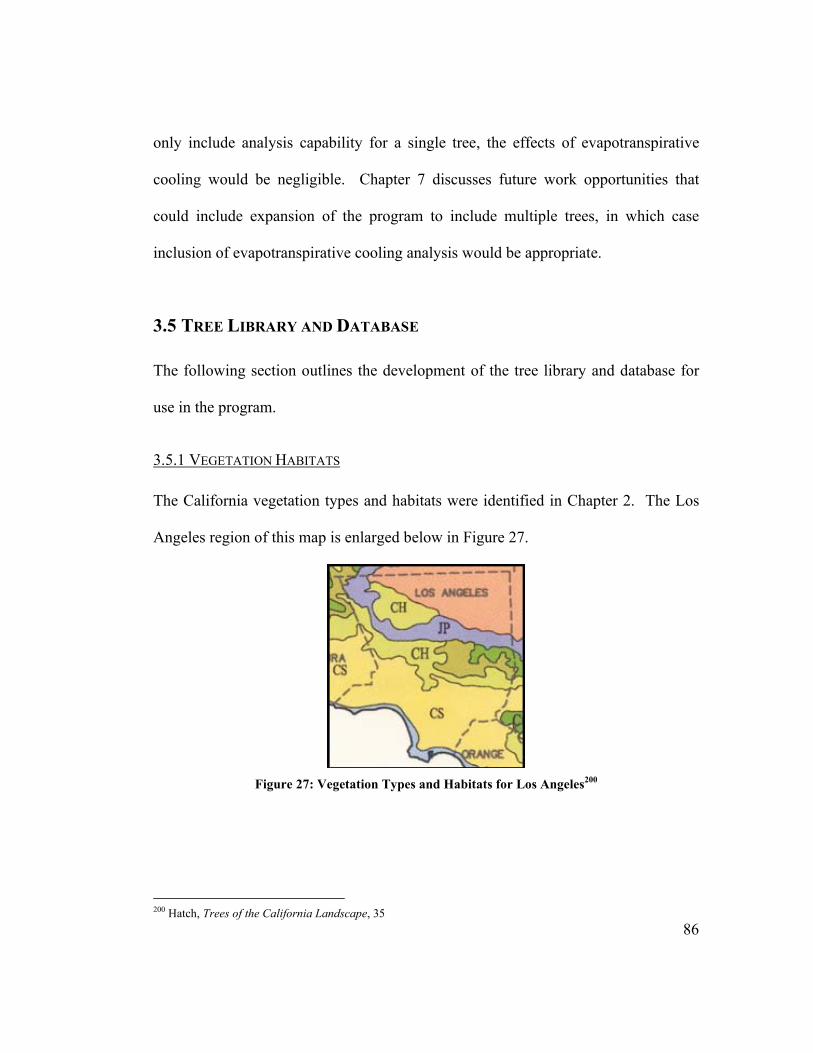
86
only include analysis capability for a single tree, the effects of evapotranspirative
cooling would be negligible. Chapter 7 discusses future work opportunities that
could include expansion of the program to include multiple trees, in which case
inclusion of evapotranspirative cooling analysis would be appropriate.
3.5 TREE LIBRARY AND DATABASE
The following section outlines the development of the tree library and database for
use in the program.
3.5.1 VEGETATION HABITATS
The California vegetation types and habitats were identified in Chapter 2. The Los
Angeles region of this map is enlarged below in Figure 27.
Figure 27: Vegetation Types and Habitats for Los Angeles200
200 Hatch, Trees of the California Landscape, 35

87
As can be seen from this map, there are 7 vegetation habitats in the Los Angeles
region: coastal strand, coastal scrub, chaparral, oak woodland, closed cone forest,
juniper-pine woodland, and Mojave Desert scrub.
3.5.1.1 Coastal Strand
Sandy beaches and dunes, with high exposure to salt spray and sand blast as well as
wind and fog, characterize the coastal strand vegetation habitat.201 The soil has low
water holding capacity as well as low organic matter content.202 These areas are
scattered along the entire length of the state, and experience typical rainfall of 15-70”
per year.
3.5.1.2 Coastal Scrub
The coastal scrub vegetation habitat is also found along the entire length of
California coast, and typically consists of coastal cliffs, bluffs, and dry gravely or
rocky slopes.203 These regions experience only 10-20” of rainfall per year.204
3.5.1.3 Chapparal
The chapparal vegetation habitat is found along the coast of California as well as
several locations inland. These areas experience rainfall of 14-25” per year.205 Dry
201 Hatch, Trees of the California Landscape, 36 202 ibid., 36 203 ibid., 38 204 ibid., 38 205 ibid., 40
88
slopes and ridges with rocky or gravely to fairly heavy soils characterize these
areas.206
3.5.1.4 Oak Woodland
The oak woodland vegetation habitat is generally found in regions similar to those of
the chapparal habitat. These regions are experience moderate temperatures and
receive about 14-25” of rainfall per year.207
3.5.1.5 Closed Cone Forest
The closed cone forest vegetation habitat is found in various locations throughout
California but is typically concentrated in Northern California. These areas consist
of coastal cliffs, bluffs, and dry gravely or rocky slopes, and experience low rainfall
(between 10-20” per year).208
3.5.1.6 Juniper-Pine Woodland
Regions of juniper-pine woodland are heavily concentrated in North-Eastern
California, but extend through Central California down to select locations in
206 Hatch, Trees of the California Landscape, 40 207 ibid., 41 208 ibid., 42

89
Southern California. These regions experience 0-30” of rainfall per year, and are
typically located in higher elevation plateau mountain regions.209
3.5.1.7 Mojave Desert Scrub
Finally, the Mojave Desert scrub vegetation habitat is located in the inland regions of
the Southern California desert. These subtropical desert regions are considered the
driest in North America, and are characterized by sandy slopes, alluvial fans, and
valleys.210 These areas experience extreme temperature fluctuations from hot to cold
and receive annual rainfall is about 2-8”.211
3.5.2 TREE DATABASE DEVELOPMENT
These vegetation habitats were used in the development of the tree library for the
computer tool. Each of these habitats has associated trees that are commonly found
in these regions.
Several sources were referenced for data on tree life span, canopy diameter,
density/transmissivity, as well as foliation period. The original list of native trees
was further refined and narrowed based on this available data. In addition, several
trees were eliminated from the library list based on ability to survive in urban
209 Hatch, Trees of the California Landscape, 42 210 ibid., 39 211 ibid., 39

90
settings. These trees were removed from the library for the purposes of this thesis
since the Los Angeles area consists mainly of highly urbanized areas, which include
the low-rise residential areas. The final list of trees that appear in the program and
their associated data are included for reference as Appendix A.

91
CHAPTER 4
The following chapter outlines in detail the method of development and operation of
the program.
4.1 WHAT THE TOOL DOES
As outlined in Chapter 1, the purpose of the tool is to provide a user with expected
savings from the planting of trees as sunshades based on simple inputs regarding the
house and tree location. The tool is designed to progress through a series of input
screens requiring the user to provide information on building and yard dimensions,
fenestration construction and location on the wall, as well as desired tree species and
its location in the yard. Once all this information has been input, the program
calculates potential reduction in incident solar radiation gain on the fenestration, and
thus the anticipated reduction in heat gain. The program will output recommended
tree locations based on anticipated reduction in instantaneous heat gain, but will also
allow the user to select where they would like to place the tree and will perform
subsequent calculations based on this input.
4.2 VISUAL BASIC
Visual Basic was selected as the program development language for several reasons.
Visual Basic 2008 is based in the .NET Framework, which is a development
environment that provides the programmer with the compiler and tools required to

92
build, debug, and execute managed applications.212 Visual Basic is an event-driven
programming language, which means that the flow or operation of the program is
determined by events (such as mouse clicks). This is suitable for the purposes of this
thesis since the execution of the program requires the user to provide inputs and
make selections that, in turn, cause the program to execute the algorithms. The
language is also recommended for novice programmers since the syntax used is
considered to be simpler than other programming languages. Despite its simplicity,
Visual Basic still allows for development of fairly complex applications. The
combination of these factors resulted in the selection Visual Basic as a suitable
platform.
4.3 DEVELOPMENT APPROACH
The development of the computer-based tool in this thesis consisted of several steps.
Since the author was required to learn the Visual Basic programming language while
conducting topic related research, two distinct but parallel paths of research and
development were required. Literature review and investigation into previously
existing simulation programs identified the need and viability of an energy efficient
landscape simulation tool. These reviews also helped to identify what information
would be required in this new tool, how it would operate, and also what outputs
212 Pelland, P, 2008, Build A Program Now: Visual Basic 2008, Microsoft, Redmond, Washington

93
would be provided to the user. Figure 28 below outlines the steps followed involved
in the development of the program.
Figure 28: Steps in Program Development
The scope and requirements were identified through the literature review process.
Subsequent to the completion of the literature review, several stand-alone programs
relating to the thesis content were developed in Visual Basic. It was intended to
learn Visual Basic while constructing the various sequences of code required in the
final program. This also aided in the design and code steps of the design. The
following sections outline the development approach in further detail.
4.3.1 SCOPE
During completion of the literature review, it was necessary to identify the scope and
purpose of the tool. It had been identified previously that, although many building
energy simulation programs were currently available, there was an apparent lack of
capability in estimating energy savings due to surrounding landscape (ie. trees). This
94
lack of availability thus helped define the purpose, scope, and boundaries for the
thesis tool.
The single-family detached home was identified as the target building type for the
tool since it was concluded that the suburban housing residential sector represented a
substantial area for reducing energy consumption.
It was originally intended to construct the tool so that it could be applied in any
location in the United States, however time constraints necessitated a narrowing of
the scope to a specific region. It was decided to focus the analytical scope of the tool
on the hot, arid region of Southern California.
4.3.2 REQUIREMENTS
Once the scope of the tool had been identified, it was necessary to determine the
requirements of the program in terms of user inputs, calculations/algorithms to be
carried out by the program, and outputs to be provided. As mentioned in Chapter 2,
the three main methods of microclimate modification by landscape involve
producing shade, acting as windbreaks, and providing evaporative cooling. These
were thus identified as the main areas of calculation analysis, which will be
transferred into algorithms. As such, the inputs, outputs, and corresponding
calculations for each of these areas were also identified. These variables are shown
in the flow chart of Figure 29 below.
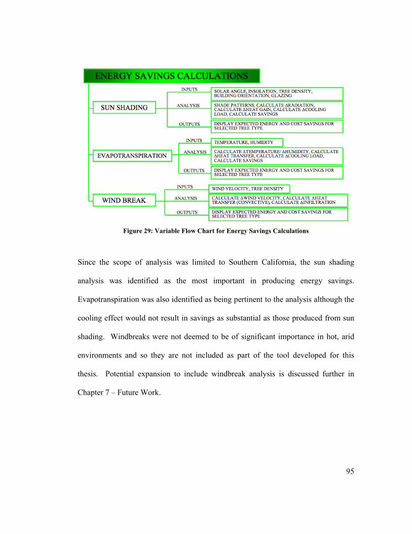
95
Figure 29: Variable Flow Chart for Energy Savings Calculations
Since the scope of analysis was limited to Southern California, the sun shading
analysis was identified as the most important in producing energy savings.
Evapotranspiration was also identified as being pertinent to the analysis although the
cooling effect would not result in savings as substantial as those produced from sun
shading. Windbreaks were not deemed to be of significant importance in hot, arid
environments and so they are not included as part of the tool developed for this
thesis. Potential expansion to include windbreak analysis is discussed further in
Chapter 7 – Future Work.

96
4.3.3 DESIGN
4.3.3.1 User Interface
Since the aim of the thesis is an interactive tool that returns outputs based on user
provided inputs, the user interface is thus a series of input screens with final screens
displaying analysis results. The development of stand-alone programs aided in the
development of the user interface as it helped to identify the variables required to be
input by the user.
Each screen consists of visual graphics, input boxes, list boxes, check boxes, and
buttons. The user is prompted to input values into the text boxes to define building
and window dimensions as well as tree placement. The list boxes provide pre-
selected window constructions, and the check boxes allow the user to select from a
list of native trees appropriate to the Los Angeles climate. Several buttons are
provided on each screen to allow the user to navigate through the program. The user
can move to the next screen, or move back to the previous screen. In the case of the
final savings output screen, additional buttons are provided to allow the user to
return to different screens to change inputs that will affect the savings results.
Finally, each screen is also provided with a help button. Clicking this button will
cause a message box to appear containing further instructions for that particular
screen, and also more detailed explanations to clarify the purpose of the inputs for
the user.

97
4.3.3.2 Program Structure
The program developed in this thesis operates in a linear manner, with each
successive screen using inputs from previous screens and obtaining information from
the user to be used later. The diagram in the figure on the following page shows a
graphical representation of the interaction between the forms, modules, and
databases.
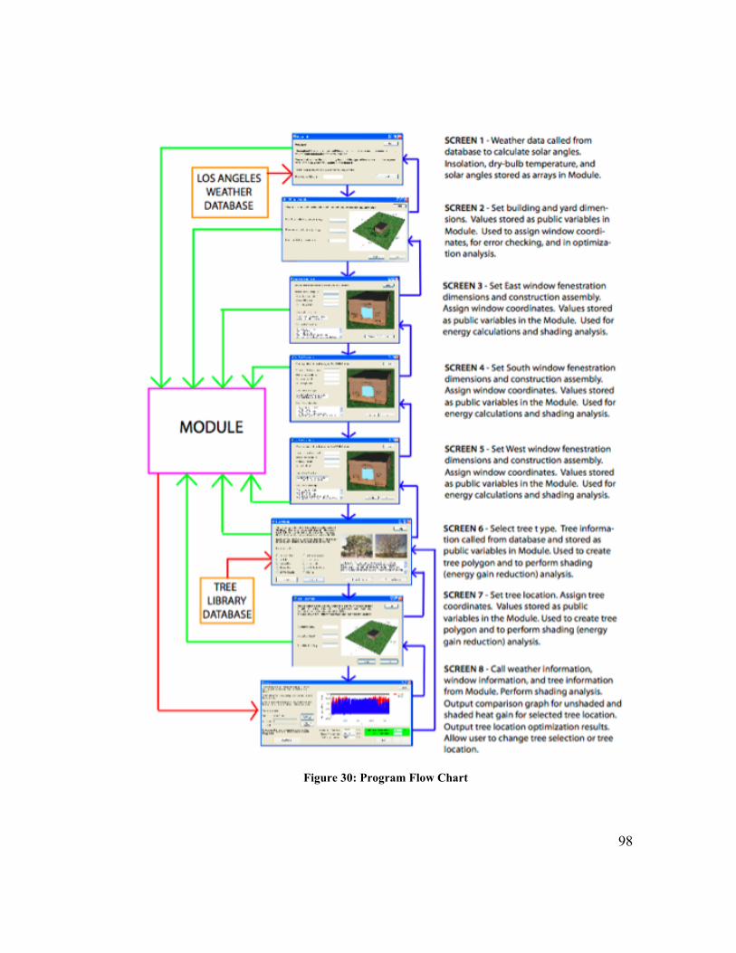
98
Figure 30: Program Flow Chart

99
4.3.4 CODE
The complete program code is included for reference as Appendix B. The following
sections outline the various elements and methods of approach used in the program
structure.
As mentioned previously, several stand-alone programs were developed in Visual
Basic to aid in the learning of the programming language itself and to gain a more
thorough understanding of the theory, calculations, and data necessary to construct
the final tool. Through development of these stand-alone programs, it was
determined that the program will consist mainly of databases, arrays, and simple
mathematical calculations. These elements are discussed in further detail in the
following sections.
4.3.4.1 Data Bases
Information required for calculations, but that is not input by the user, is stored and
called from an organized collection of information stored within the program known
as a database.213 The database is available whenever the user runs the program.
Information is called from the database depending on the user inputs and is
transferred to the main algorithms as a dataset to be temporarily stored as variables
or in an array. This temporary storage allows the program to use the information in
213 Halvorson, M, Visual Basic 2008 Step by Step, Microsoft, Redmond, Washington
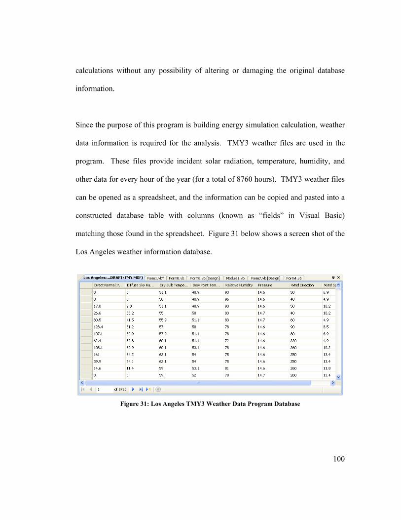
100
calculations without any possibility of altering or damaging the original database
information.
Since the purpose of this program is building energy simulation calculation, weather
data information is required for the analysis. TMY3 weather files are used in the
program. These files provide incident solar radiation, temperature, humidity, and
other data for every hour of the year (for a total of 8760 hours). TMY3 weather files
can be opened as a spreadsheet, and the information can be copied and pasted into a
constructed database table with columns (known as “fields” in Visual Basic)
matching those found in the spreadsheet. Figure 31 below shows a screen shot of the
Los Angeles weather information database.
Figure 31: Los Angeles TMY3 Weather Data Program Database
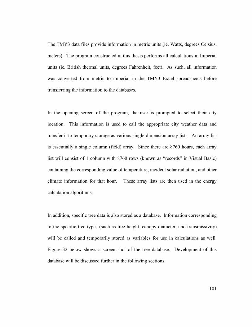
101
The TMY3 data files provide information in metric units (ie. Watts, degrees Celsius,
meters). The program constructed in this thesis performs all calculations in Imperial
units (ie. British thermal units, degrees Fahrenheit, feet). As such, all information
was converted from metric to imperial in the TMY3 Excel spreadsheets before
transferring the information to the databases.
In the opening screen of the program, the user is prompted to select their city
location. This information is used to call the appropriate city weather data and
transfer it to temporary storage as various single dimension array lists. An array list
is essentially a single column (field) array. Since there are 8760 hours, each array
list will consist of 1 column with 8760 rows (known as “records” in Visual Basic)
containing the corresponding value of temperature, incident solar radiation, and other
climate information for that hour. These array lists are then used in the energy
calculation algorithms.
In addition, specific tree data is also stored as a database. Information corresponding
to the specific tree types (such as tree height, canopy diameter, and transmissivity)
will be called and temporarily stored as variables for use in calculations as well.
Figure 32 below shows a screen shot of the tree database. Development of this
database will be discussed further in the following sections.
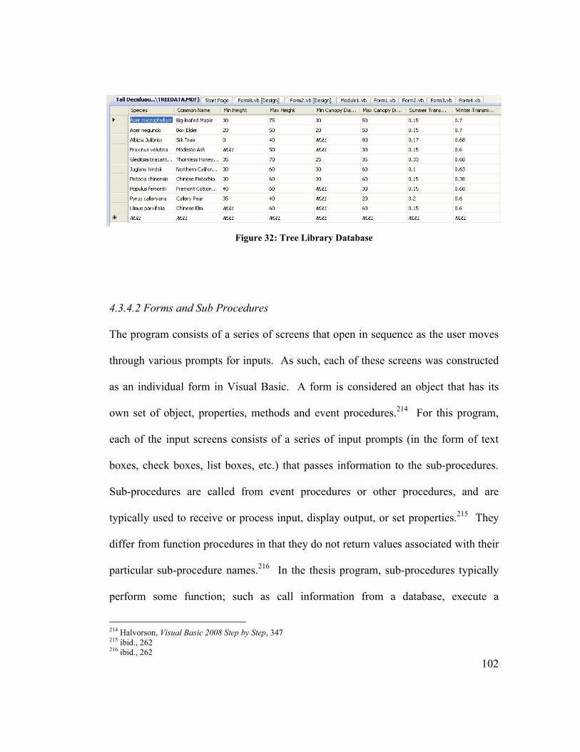
102
Figure 32: Tree Library Database
4.3.4.2 Forms and Sub Procedures
The program consists of a series of screens that open in sequence as the user moves
through various prompts for inputs. As such, each of these screens was constructed
as an individual form in Visual Basic. A form is considered an object that has its
own set of object, properties, methods and event procedures.214 For this program,
each of the input screens consists of a series of input prompts (in the form of text
boxes, check boxes, list boxes, etc.) that passes information to the sub-procedures.
Sub-procedures are called from event procedures or other procedures, and are
typically used to receive or process input, display output, or set properties.215 They
differ from function procedures in that they do not return values associated with their
particular sub-procedure names.216 In the thesis program, sub-procedures typically
perform some function; such as call information from a database, execute a
214 Halvorson, Visual Basic 2008 Step by Step, 347 215 ibid., 262 216 ibid., 262

103
calculation, or return a variable. Variables are a type of container used to temporarily
hold data in the program.217 Variables are declared or created and are subsequently
used to store names, inputs, and to help perform and store results of calculations.
4.3.4.3 Modules
Since the program requires the use of multiple forms, it is necessary to define global
variables that can be used throughout the program. When variables or sub functions
are defined in a form, they can only be used in that form. This is problematic for the
format of this program since the various forms require access to the same
information (ie. variables). As such, specific variables or arrays that are required
throughout the program were identified and declared as public variables in a module.
A module is a special file that contains variable declarations and procedures that can
be used anywhere in the program.218 This is useful for the type of analysis
performed in this program since the various algorithms use information obtained in
the different user input screens and conduct hourly energy simulation analysis. As
such, the variables used are required for different equations in different forms, and
also the value of the variables change with the hourly analysis.
217 Halvorson, Visual Basic 2008 Step by Step, 80 218 ibid., 254

104
4.4 METHOD OF OPERATION
The following section outlines the function of the program. Each form will be
discussed in detail, outlining how the various inputs call database information or are
used in the algorithms. The outputs of these algorithms will also be discussed.
4.4.1 SCREEN 1 – WELCOME SCREEN
When the program is opened, the user is greeted with the welcome screen, as shown
below in Figure 33. On this same screen, the user is prompted to input information
on their local electrical utility rate.
Figure 33: Program Welcome Screen
Since the scope of the program is limited to Los Angeles, clicking the “Next” button
provides the necessary event sequence to cause the program to call the required
weather data from the database (Figure 34 below).

105
Figure 34: User Input Relation to Los Angeles Weather Database
The right side of the image above shows the Los Angeles Dataset. The Los Angles
Table Adapter allows the data to be accessed and transferred as a dataset from the
database. When the desired data is accessed from the database, it is transferred to the
program for use in what is known as a dataset. The dataset is simply a copy of the
data that is stored in the database and contains the values that will be used by the
program. This allows the data to be used or manipulated in calculations without the
potential of the original data in the database being altered or erased. A small sub-
function in this form transfers the direct normal irradiance and dry bulb temperature
data into two separate single-field array lists (to be used in calculations).
The “Next” button click event also executes a sub function in this form that assigns
appropriate latitude and longitude values for the location. Finally, this form executes
another sub-function that calculates the solar angles (azimuth and altitude) for each
hour of the year based on the latitude and longitude. As mentioned in Chapter 2, the
azimuth angle is assigned a positive or negative sign depending on the time of day.
This sign convention is established based on the matrix transformation equations but
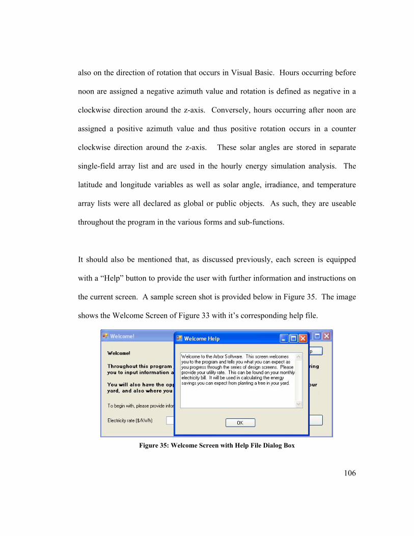
106
also on the direction of rotation that occurs in Visual Basic. Hours occurring before
noon are assigned a negative azimuth value and rotation is defined as negative in a
clockwise direction around the z-axis. Conversely, hours occurring after noon are
assigned a positive azimuth value and thus positive rotation occurs in a counter
clockwise direction around the z-axis. These solar angles are stored in separate
single-field array list and are used in the hourly energy simulation analysis. The
latitude and longitude variables as well as solar angle, irradiance, and temperature
array lists were all declared as global or public objects. As such, they are useable
throughout the program in the various forms and sub-functions.
It should also be mentioned that, as discussed previously, each screen is equipped
with a “Help” button to provide the user with further information and instructions on
the current screen. A sample screen shot is provided below in Figure 35. The image
shows the Welcome Screen of Figure 33 with it’s corresponding help file.
Figure 35: Welcome Screen with Help File Dialog Box
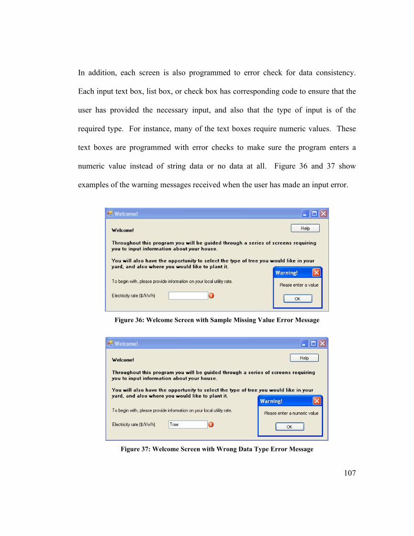
107
In addition, each screen is also programmed to error check for data consistency.
Each input text box, list box, or check box has corresponding code to ensure that the
user has provided the necessary input, and also that the type of input is of the
required type. For instance, many of the text boxes require numeric values. These
text boxes are programmed with error checks to make sure the program enters a
numeric value instead of string data or no data at all. Figure 36 and 37 show
examples of the warning messages received when the user has made an input error.
Figure 36: Welcome Screen with Sample Missing Value Error Message
Figure 37: Welcome Screen with Wrong Data Type Error Message
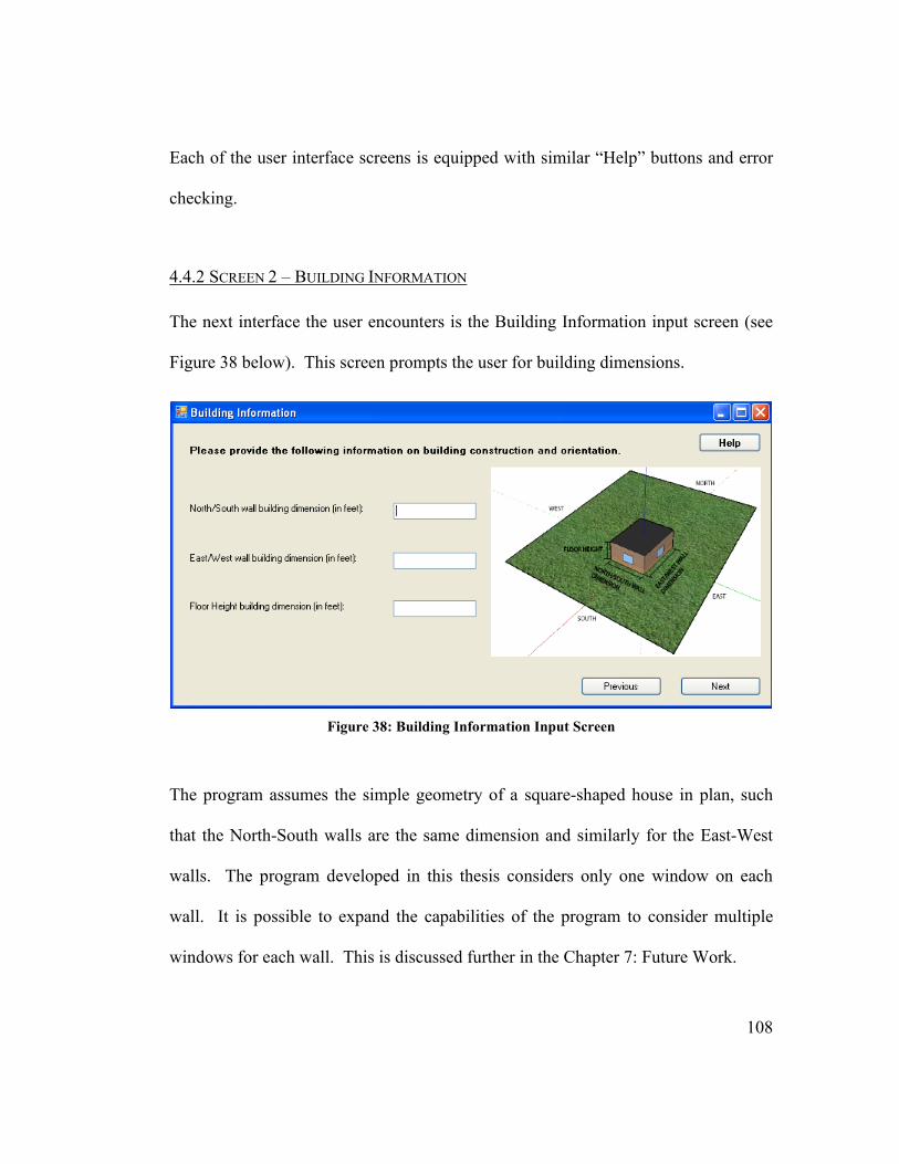
108
Each of the user interface screens is equipped with similar “Help” buttons and error
checking.
4.4.2 SCREEN 2 – BUILDING INFORMATION
The next interface the user encounters is the Building Information input screen (see
Figure 38 below). This screen prompts the user for building dimensions.
Figure 38: Building Information Input Screen
The program assumes the simple geometry of a square-shaped house in plan, such
that the North-South walls are the same dimension and similarly for the East-West
walls. The program developed in this thesis considers only one window on each
wall. It is possible to expand the capabilities of the program to consider multiple
windows for each wall. This is discussed further in the Chapter 7: Future Work.
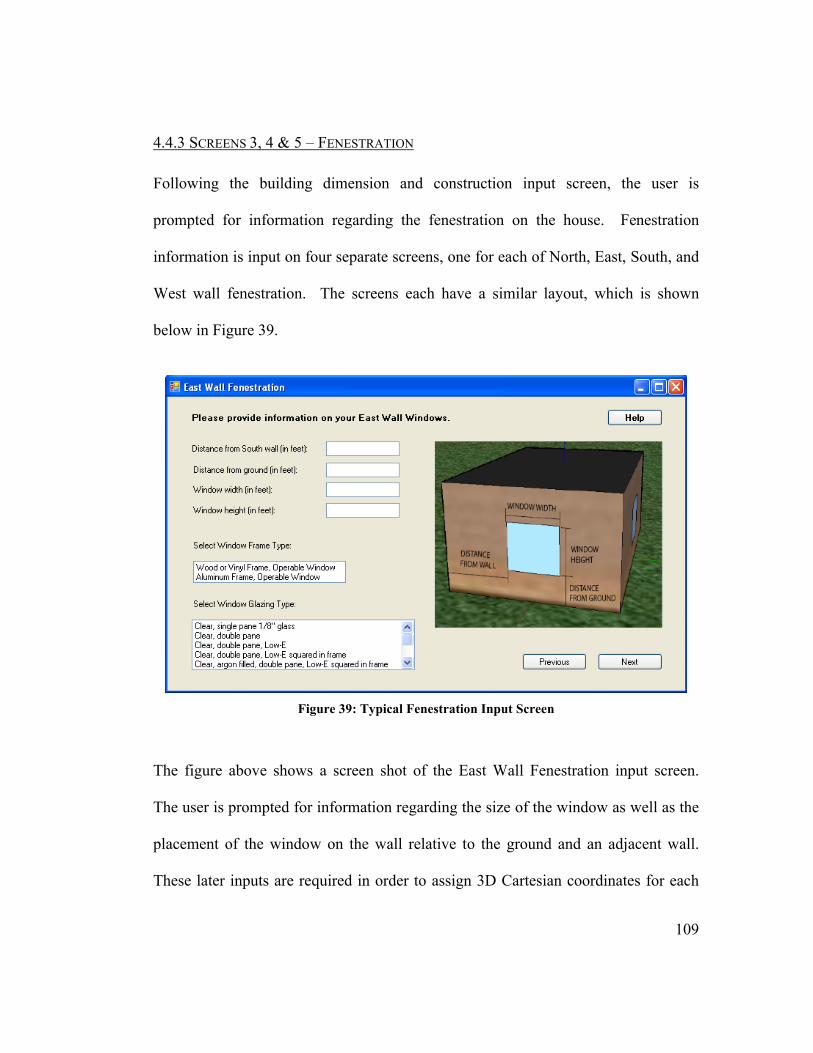
109
4.4.3 SCREENS 3, 4 & 5 – FENESTRATION
Following the building dimension and construction input screen, the user is
prompted for information regarding the fenestration on the house. Fenestration
information is input on four separate screens, one for each of North, East, South, and
West wall fenestration. The screens each have a similar layout, which is shown
below in Figure 39.
Figure 39: Typical Fenestration Input Screen
The figure above shows a screen shot of the East Wall Fenestration input screen.
The user is prompted for information regarding the size of the window as well as the
placement of the window on the wall relative to the ground and an adjacent wall.
These later inputs are required in order to assign 3D Cartesian coordinates for each

110
of the 4 corners of the window. The user is also required to select the frame and
glazing type of the window. These are selected from the list boxes shown on the
bottom left of the image. Depending on the frame and glazing combination selected,
the program assigns a U-value and Solar Heat Gain Coefficient to the window.
These values are required to calculate the instantaneous heat gain.
4.4.4 SCREEN 6 – TREE SELECTION
Once all required the user has provided all required building information, the
remaining input screens offer the opportunity to select from a list of trees. Figure 40
below shows an image of screen 6, which allows the user to select from a list of tall
deciduous trees.
Figure 40: Tree Selection Input Screen
The user selects from a pre-determined short list of climate appropriate deciduous
trees. Once the user clicks one of the radio buttons and clicks the “Select Tree”
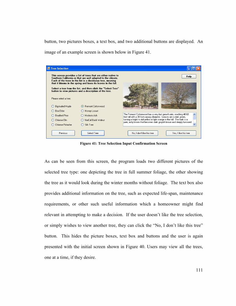
111
button, two pictures boxes, a text box, and two additional buttons are displayed. An
image of an example screen is shown below in Figure 41.
Figure 41: Tree Selection Input Confirmation Screen
As can be seen from this screen, the program loads two different pictures of the
selected tree type: one depicting the tree in full summer foliage, the other showing
the tree as it would look during the winter months without foliage. The text box also
provides additional information on the tree, such as expected life-span, maintenance
requirements, or other such useful information which a homeowner might find
relevant in attempting to make a decision. If the user doesn’t like the tree selection,
or simply wishes to view another tree, they can click the “No, I don’t like this tree”
button. This hides the picture boxes, text box and buttons and the user is again
presented with the initial screen shown in Figure 40. Users may view all the trees,
one at a time, if they desire.
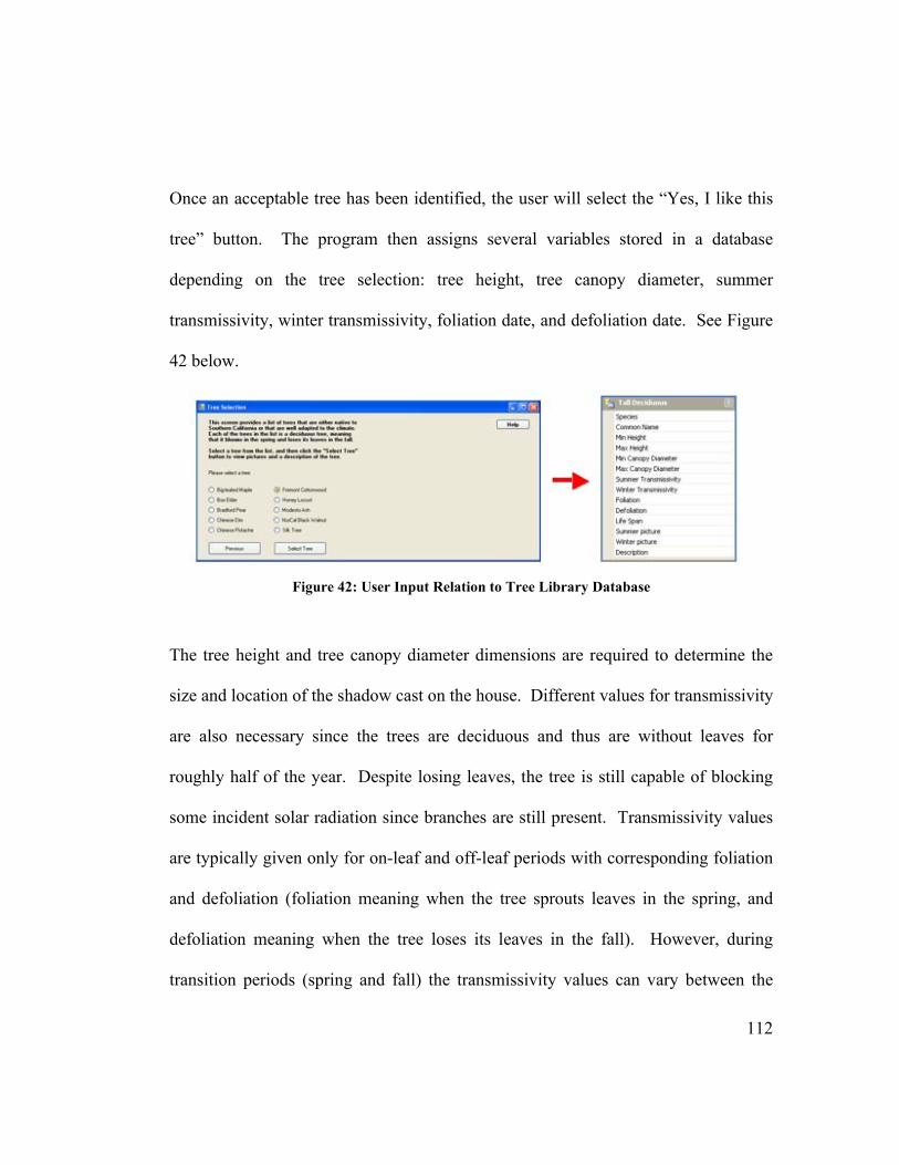
112
Once an acceptable tree has been identified, the user will select the “Yes, I like this
tree” button. The program then assigns several variables stored in a database
depending on the tree selection: tree height, tree canopy diameter, summer
transmissivity, winter transmissivity, foliation date, and defoliation date. See Figure
42 below.
Figure 42: User Input Relation to Tree Library Database
The tree height and tree canopy diameter dimensions are required to determine the
size and location of the shadow cast on the house. Different values for transmissivity
are also necessary since the trees are deciduous and thus are without leaves for
roughly half of the year. Despite losing leaves, the tree is still capable of blocking
some incident solar radiation since branches are still present. Transmissivity values
are typically given only for on-leaf and off-leaf periods with corresponding foliation
and defoliation (foliation meaning when the tree sprouts leaves in the spring, and
defoliation meaning when the tree loses its leaves in the fall). However, during
transition periods (spring and fall) the transmissivity values can vary between the
113
winter and summer values. Program code was altered to assign a varying
transmissivity value over the course of a month surrounding the foliation and
defoliation dates to reflect the slow appearance or disappearance of tree foliage.
Transmissivity values are different for each tree species, as are foliation and
defoliation dates since the varying species of trees sprout and lose leaves at different
times. Finally, this button click also provides the event that opens up the final user
input screen.
4.4.5 SCREEN 7 - TREE PLACEMENT
Once a tree has been selected from the library, the user may select where they wish
to place the tree in the yard. Inputs are required in relation to the x, y, z coordinate
system, as shown below in Figure 43.
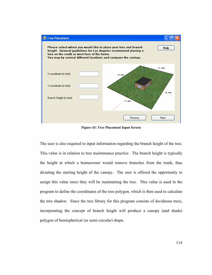
114
Figure 43: Tree Placement Input Screen
The user is also required to input information regarding the branch height of the tree.
This value is in relation to tree maintenance practice. The branch height is typically
the height at which a homeowner would remove branches from the trunk, thus
dictating the starting height of the canopy. The user is offered the opportunity to
assign this value since they will be maintaining the tree. This value is used in the
program to define the coordinates of the tree polygon, which is then used to calculate
the tree shadow. Since the tree library for this program consists of deciduous trees,
incorporating the concept of branch height will produce a canopy (and shade)
polygon of hemispherical (or semi-circular) shape.
115
4.4.5.1 Construction of Tree Polygon
The tree polygon is constructed using the values for tree canopy diameter (called
from the data base) as well as the user-defined input of branch height. These values
are used in conjunction with a pre-determined polygon point array to establish the
proper polygon shape for the tree selected. The pre-determined polygon point array
consists of 40 points, each with (x,y,z) coordinates, defining various locations of the
tree trunk as well as canopy. The polygon point array is scaled to a value of 1, thus
the selected tree branch height and tree canopy diameter are used as multipliers to
determine the points for the particular tree. Sine and cosine calculations are used to
determine the coordinates of each point.
4.4.5.2 Recommended Tree Placement
Since the program is designed for evaluation in the Los Angeles region, it is
recommended to place a single tree to the west or southwest exterior windows in
order to achieve maximum benefits from available shade.219 The user is provided
with this recommendation on the tree placement screen.
Clicking on the “Next” button also executes the code that performs the hourly
shading analyses for each wall. This code includes the scanline algorithms and
instantaneous heat gain calculations and is discussed in further detail in the following
section.
219 McPherson et al., Potential of Tree Shade for Reducing Residential Energy Use in California, 16
116
4.4.6 SCANLINE ALGORITHM & INSTANTANEOUS COOLING LOAD CALCULATIONS
Two separate sets of cooling load calculations are performed for each window:
instantaneous loads without shade and instantaneous loads with (if any) shade. Both
sets of calculations are performed hourly based on TMY3 data using values for direct
normal irradiation. The instantaneous load calculations without shade are performed
using the same value for direct normal irradiation, given for the particular hour, over
the entire area of the window (which is derived using the window height and
diameter provided by the user). The instantaneous load calculations that consider
shading from the tree incorporate a scanline algorithm to determine which portions
of the window are in shade and thus which portions are receiving less direct normal
irradiation due to this shade.
As mentioned previously, the building is rotated for each hour so it is inline with the
sun. The surface solar azimuth calculation for each wall plane is then performed to
determine if the plane is facing the sun. If it is, it is included in the shading analysis
for that hour. If not, it is discarded from the analysis for that particular hour. If the
wall plane is included in the analysis for that hour, the scanline algorithm performs
the analysis for the window on that plane (the window coordinates are also rotated).
The tree shadow on the window is also simplified via the matrix rotations. The
interaction between the two becomes a simple overlapping of polygons: the square
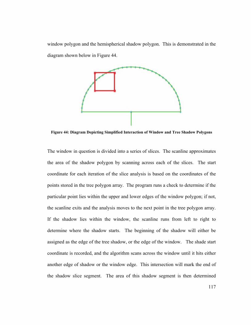
117
window polygon and the hemispherical shadow polygon. This is demonstrated in the
diagram shown below in Figure 44.
Figure 44: Diagram Depicting Simplified Interaction of Window and Tree Shadow Polygons
The window in question is divided into a series of slices. The scanline approximates
the area of the shadow polygon by scanning across each of the slices. The start
coordinate for each iteration of the slice analysis is based on the coordinates of the
points stored in the tree polygon array. The program runs a check to determine if the
particular point lies within the upper and lower edges of the window polygon; if not,
the scanline exits and the analysis moves to the next point in the tree polygon array.
If the shadow lies within the window, the scanline runs from left to right to
determine where the shadow starts. The beginning of the shadow will either be
assigned as the edge of the tree shadow, or the edge of the window. The shade start
coordinate is recorded, and the algorithm scans across the window until it hits either
another edge of shadow or the window edge. This intersection will mark the end of
the shadow slice segment. The area of this shadow segment is then determined
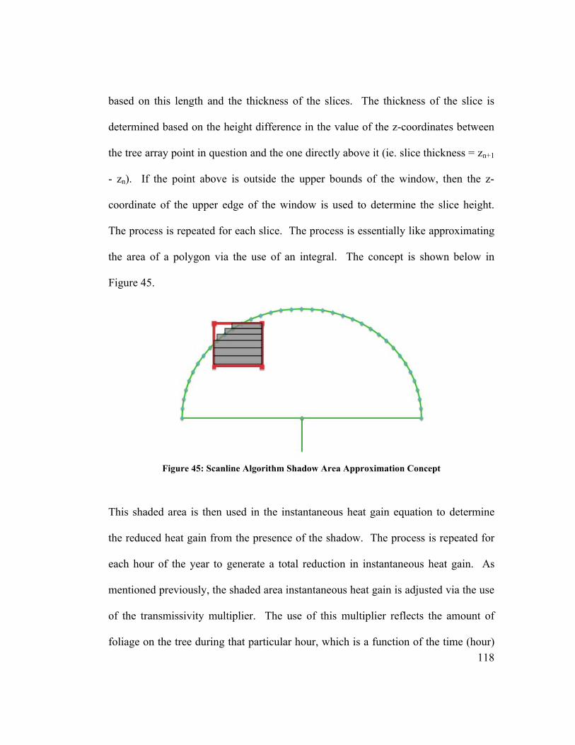
118
based on this length and the thickness of the slices. The thickness of the slice is
determined based on the height difference in the value of the z-coordinates between
the tree array point in question and the one directly above it (ie. slice thickness = zn+1
- zn). If the point above is outside the upper bounds of the window, then the z-
coordinate of the upper edge of the window is used to determine the slice height.
The process is repeated for each slice. The process is essentially like approximating
the area of a polygon via the use of an integral. The concept is shown below in
Figure 45.
Figure 45: Scanline Algorithm Shadow Area Approximation Concept
This shaded area is then used in the instantaneous heat gain equation to determine
the reduced heat gain from the presence of the shadow. The process is repeated for
each hour of the year to generate a total reduction in instantaneous heat gain. As
mentioned previously, the shaded area instantaneous heat gain is adjusted via the use
of the transmissivity multiplier. The use of this multiplier reflects the amount of
foliage on the tree during that particular hour, which is a function of the time (hour)

119
of the year. Incorporating transmissivity into the analysis allows for more accurate
representation of the shading effects of trees. It is also possible to use the scanline
algorithm for analyzing the shade patterns from the presence of more than one tree.
The scanline would run across each slice and would allow for the adjustment of
transmissivity should multiple shade polygons overlap each other. Since the
program developed in this thesis considers only one tree, the expansion to consider
multiple trees is possible, and is included in the Future Work discussion in Chapter
7.
As can be seen from Figure 45, the slices decrease in height near the top of the tree
canopy. This results in a slight variation in degree of accuracy along the height of
the window since the points are spaced more closely together at one end. This
method is dependent on the number of points assigned to create the tree array. The
degree of accuracy could be improved by assigning a small constant slice height or
increases the number of points that define the array, since smaller slices in greater
numbers would more closely approximate the curve of the tree shadow polygon. The
method of using the tree points produces acceptable results, and so it was decided to
keep this approach since the tree canopy array was already constructed and so could
be used for multiple purposes.
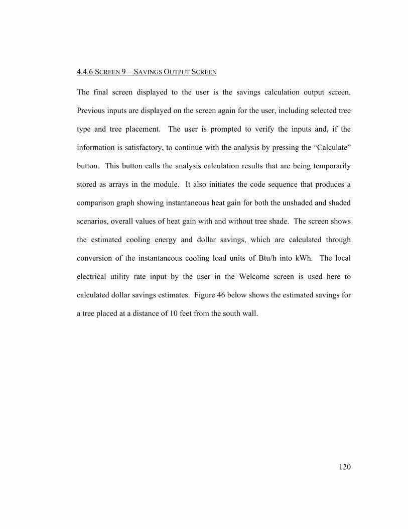
120
4.4.6 SCREEN 9 – SAVINGS OUTPUT SCREEN
The final screen displayed to the user is the savings calculation output screen.
Previous inputs are displayed on the screen again for the user, including selected tree
type and tree placement. The user is prompted to verify the inputs and, if the
information is satisfactory, to continue with the analysis by pressing the “Calculate”
button. This button calls the analysis calculation results that are being temporarily
stored as arrays in the module. It also initiates the code sequence that produces a
comparison graph showing instantaneous heat gain for both the unshaded and shaded
scenarios, overall values of heat gain with and without tree shade. The screen shows
the estimated cooling energy and dollar savings, which are calculated through
conversion of the instantaneous cooling load units of Btu/h into kWh. The local
electrical utility rate input by the user in the Welcome screen is used here to
calculated dollar savings estimates. Figure 46 below shows the estimated savings for
a tree placed at a distance of 10 feet from the south wall.
121
Figure 46: Savings Output Screen
From here, the user has the option of performing another analysis by selecting a
different tree or changing the tree location. The user can perform as many iterations
of the analysis as they like since the program will execute a new shading analysis
each time.
The program developed in this thesis proceeds through simple input screens in a
linear manner, requiring basic inputs from the user. The following two chapters
(Chapters 5 and 6) contain a detailed discussion of validation analyses of program
code, calculations and results that were performed to verify the accuracy of
information provided to the user on the savings output screen.
122
CHAPTER 5 The following chapter outlines several approaches used in the verification of the
results output by the computer program. Verification processes were used to
evaluate the results output by the program, and also to ensure that, prior to output
evaluation, each section of code was functioning properly. Results were compared
to those results output by other software packages, as well as to expected percentage
savings outlined in other research publications.
5.1 VERIFICATION OF PROGRAM CODE
Once each section of the program was written, it was necessary to verify that the
code was working as intended. The process of debugging involved detailed error
checking of each step to ensure that all calculated values and analyses were
functioning. The Visual Basic Message Box function was often used to display
values called from databases or to display results of various calculations. Microsoft
Excel was also used in several instances to evaluate results of calculations.
5.1.1 VERIFICATION OF TREE POLYGON CONSTRUCTION CODE
Microsoft Excel was used in the verification of the tree polygon construction code to
check that values were being calculated correctly and also to ensure that the shape of
the tree polygon was semicircular. A sample tree canopy diameter of 15 feet, and a
sample branch height of 7 feet were used. The points of the tree canopy are found
using the tree radius along with cosine and sine functions to find x- and z-
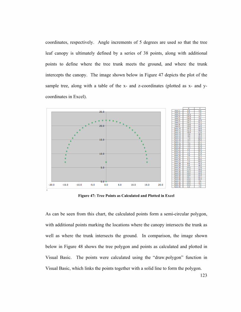
123
coordinates, respectively. Angle increments of 5 degrees are used so that the tree
leaf canopy is ultimately defined by a series of 38 points, along with additional
points to define where the tree trunk meets the ground, and where the trunk
intercepts the canopy. The image shown below in Figure 47 depicts the plot of the
sample tree, along with a table of the x- and z-coordinates (plotted as x- and y-
coordinates in Excel).
Figure 47: Tree Points as Calculated and Plotted in Excel
As can be seen from this chart, the calculated points form a semi-circular polygon,
with additional points marking the locations where the canopy intersects the trunk as
well as where the trunk intersects the ground. In comparison, the image shown
below in Figure 48 shows the tree polygon and points as calculated and plotted in
Visual Basic. The points were calculated using the “draw.polygon” function in
Visual Basic, which links the points together with a solid line to form the polygon.

124
Figure 48: Tree Polygon As Plotted in Visual Basic
The image in Figure 48 shows just the semi-circle of the tree canopy. The thesis
program does define additional points for the trunk (base) of the tree, however they
were not included in the draw.polygon code.
5.1.2 VERIFICATION OF SCANLINE ALGORITHM CODE
The performance of the scanline algorithm was also verified with the use of
Microsoft Excel. A square box of 6 x 6 dimensions was plotted along with the tree
polygon. The square window polygon was moved around to various locations to test
the performance of the algorithm by comparing calculated values in Excel versus
those in Visual Basic. Shade values were calculated for each scanline slice, and the
total shaded area was calculated as the sum of these shade area slices. Figures 49
and 50 below show a sample scanline verification test. The window polygon was
placed at the very left of the tree polygon, so that the bottom left point was at the
same x-coordinate as the tree radius and same z-coordinate as the branch height. The
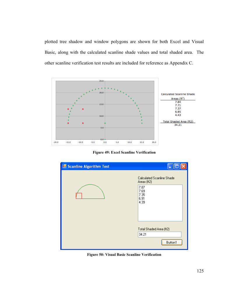
125
plotted tree shadow and window polygons are shown for both Excel and Visual
Basic, along with the calculated scanline shade values and total shaded area. The
other scanline verification test results are included for reference as Appendix C.
Figure 49: Excel Scanline Verification
Figure 50: Visual Basic Scanline Verification
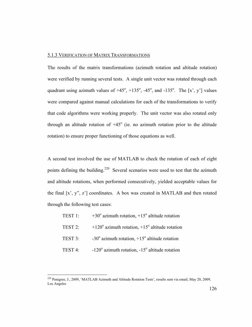
126
5.1.3 VERIFICATION OF MATRIX TRANSFORMATIONS
The results of the matrix transformations (azimuth rotation and altitude rotation)
were verified by running several tests. A single unit vector was rotated through each
quadrant using azimuth values of +45o, +135o, -45o, and -135o. The [x’, y’] values
were compared against manual calculations for each of the transformations to verify
that code algorithms were working properly. The unit vector was also rotated only
through an altitude rotation of +45o (ie. no azimuth rotation prior to the altitude
rotation) to ensure proper functioning of those equations as well.
A second test involved the use of MATLAB to check the rotation of each of eight
points defining the building.220 Several scenarios were used to test that the azimuth
and altitude rotations, when performed consecutively, yielded acceptable values for
the final [x’, y”, z’] coordinates. A box was created in MATLAB and then rotated
through the following test cases:
TEST 1: +30o azimuth rotation, +15o altitude rotation
TEST 2: +120o azimuth rotation, +15o altitude rotation
TEST 3: -30o azimuth rotation, +15o altitude rotation
TEST 4: -120o azimuth rotation, -15o altitude rotation
220 Penigree, J., 2009, ‘MATLAB Azimuth and Altitude Rotation Tests’, results sent via email, May 20, 2009, Los Angeles
127
These points were then check against outputs of the matrix transformation code in
the program. The purpose of performing four separate tests is to ensure that the
azimuth and altitude transformations operate as expected through a range of possible
rotations. Employing MATLAB is also valuable since MATLAB rotates the object
only, as opposed to the possibility of rotating the axes. By comparing the program
outputs to those of MATLAB, it is possible to confirm the rotations that are
occurring in Visual Basic.
A final test was used to verify that both the matrix transformations and scanline
algorithm was working. This test involved a simple calculation that relates tree
height, tree distance from the house, and the tangent of the altitude angle. The
equation is as follows221:
h = y tan(Alt) (26)
where: h = height of the top of the tree from the ground (ft) y = distance from tree to the wall plane (ft) Alt = solar altitude angle
Assuming the height of the tree is known, the equation can also be written as
y =h
tan(Alt) (27)
For this verification test equation (27) was used since it was assumed that the tree
height was known. To simplify the analysis, the windowsill and base of the tree
221 Moffat et al., Landscape Design That Saves Energy, 119

128
canopy were dropped to the ground. Using a tree canopy diameter of 30 feet, the
height of the treetop from the ground was assumed as the tree radius, or half the tree
canopy diameter (ie. 15 feet). The solar altitude angle was assumed to be 30o. Thus
the calculated distance from the wall plane to the tree was about 26 feet. This is the
distance the tree would need to be in order for the sun to have a “clear view” of the
window at an altitude angle of 30o. In other words, at this tree distance there would
be no shade on the window if the sun were at an altitude of 30o. This scenario was
tested for the east, south, and west walls. In each test case, the tree was placed
directly adjacent to the wall plane in question at a distance of 26 feet. For each wall,
the appropriate azimuth rotation was performed to bring the sun in line with the wall.
For example, an azimuth rotation of -90o was performed for the east wall, 0o for the
south wall, and +90o for the west wall. Following the azimuth rotation, three
separate altitude transformations were performed. One rotation was performed at
28o, the second at 30o, and the last at 32o. A properly functioning matrix
transformation would yield a small percentage of window in shade at 28o and no
window in shade at both 30o and 32o. The test was performed successfully for all
three walls.
5.1.4 VERIFICATION OF TRANSMISSIVITY MULTIPLIER
As mentioned previously, a transmissivity multiplier is applied to the instantaneous
heat gain calculations for the scenarios in which the window is shaded by the tree.
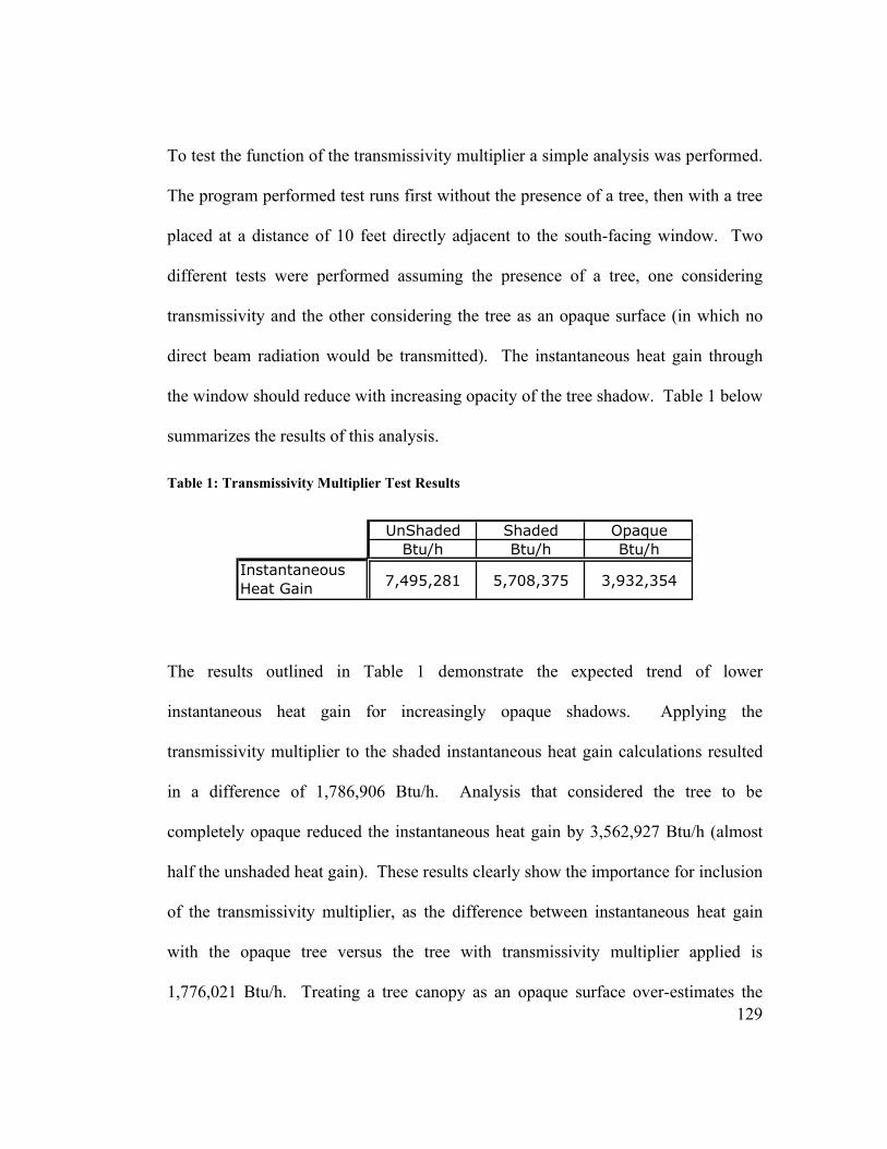
129
To test the function of the transmissivity multiplier a simple analysis was performed.
The program performed test runs first without the presence of a tree, then with a tree
placed at a distance of 10 feet directly adjacent to the south-facing window. Two
different tests were performed assuming the presence of a tree, one considering
transmissivity and the other considering the tree as an opaque surface (in which no
direct beam radiation would be transmitted). The instantaneous heat gain through
the window should reduce with increasing opacity of the tree shadow. Table 1 below
summarizes the results of this analysis.
Table 1: Transmissivity Multiplier Test Results
The results outlined in Table 1 demonstrate the expected trend of lower
instantaneous heat gain for increasingly opaque shadows. Applying the
transmissivity multiplier to the shaded instantaneous heat gain calculations resulted
in a difference of 1,786,906 Btu/h. Analysis that considered the tree to be
completely opaque reduced the instantaneous heat gain by 3,562,927 Btu/h (almost
half the unshaded heat gain). These results clearly show the importance for inclusion
of the transmissivity multiplier, as the difference between instantaneous heat gain
with the opaque tree versus the tree with transmissivity multiplier applied is
1,776,021 Btu/h. Treating a tree canopy as an opaque surface over-estimates the
UnShaded Shaded Opaque
Btu/h Btu/h Btu/h
Instantaneous
Heat Gain7,495,281 5,708,375 3,932,354
130
amount of savings that can be achieved since it does not accurate model the
insolation filtering effects of tree canopies.
5.2 COMPARISON TO HEED
5.2.1 OVERVIEW OF HEED
HEED (Home Energy Efficient Design) is a software program developed through the
University of California Los Angeles to aid designers in making specific changes to
a residential building design to reduce the energy consumption within the
building.222 The user can draw the floor plan of their house, design and place
windows and doors, as well as select various construction assemblies and mechanical
systems. Advanced options involve definition of interior building loads (including
appliances and lighting) as well as offering the option of defining building
occupancy. The user may create several iterations of their building design to
determine what effect changing certain options (such as window construction or wall
insulation) has on the building performance. Outputs are given as values of energy
consumption (Btu/h or Btu/h*ft2) or as dollar amounts ($/ft2). Several graphics are
also provided for the user in the form of bar graphs showing the difference between
design iterations, as well as 3D plots of variables such as indoor temperature or peak
load over an annual period.
222 University of California Los Angeles, HEED: Home Energy Efficiency Design, University of California Los Angeles, viewed January 2008, http://mackintosh.aud.ucla.edu/heed/
131
5.2.2 COMPARISON OF THESIS PROGRAM TO HEED
The program developed in this thesis is similar to HEED in that both are designed for
analysis of residential buildings. HEED offers the user the capability of defining a 1
or 2 story house, and provides an intuitive user interface through the user of
interactive graphics. The program developed in this thesis is also currently limited to
instantaneous heat gain analysis through fenestration surfaces only, with
corresponding estimates of energy savings, whereas HEED performs an entire
building consumption and load profile analysis. HEED does offer some analysis for
exterior shading devices, but does not, however, currently include any analysis for
consideration of landscape elements.
5.2.2.1 HEED Heat Gain Calculations
Heat gain (or loss) is calculated in HEED as follows. HEED considers conduction
gain or loss through fenestration surfaces, and adds to this the direct radiation
multiplied by the solar heat gain coefficient (corrected to angle of incidence) plus the
diffuse radiation times solar heat gain coefficient. The equation is shown below:
Q =U A (Tout Tin ) + SHGC Area (DirectBeam cos + Diffuse) (28)
where: Q = Energy gain/loss (Btu/h) U = overall coefficient of heat transfer (Btu/h*ft2*oF) A = total area of fenestration, ft2 Tout = exterior air temperature (oF) Tin = interior air temperature (oF) Direct = incident direct beam radiation (Btu/h*ft2)
132
Diffuse = diffuse sky radiation (Btu/h*ft2) = angle of incidence (degrees)
SHGC = solar heat gain coefficient
The above equation is similar to that used in the thesis program since both consider
conduction and radiation heat gain. Both programs use TMY3 weather data,
although HEED uploads the data in EPW. file format. The HEED calculation,
however, considers the added radiation heat gain from diffuse radiation. The
calculation in the thesis program uses TMY3 data for direct normal irradiance only,
which is the amount of radiation received in a collimated beam on a surface normal
to the sun’s rays.223
5.2.3 THESIS PROGRAM AND HEED INPUTS
In order to verify and compare the outputs of the thesis program versus those of
HEED, similar buildings and fenestration surfaces must first be constructed in each
of the programs.
5.2.3.1 Building Dimension and Fenestration
The buildings modelled in the thesis program as well as HEED are roughly square-
shaped single-story homes with an area of approximately 2,000 square feet. The
north-south walls are the same dimension, and the east-west walls are also the same
223 National Renewable Energy Laboratory, 2008, Users Manual for TMY3 Data Sets, United States Department of Energy Office of Energy Efficiency & Renewable Energy, viewed October 2008, http://www.nrel.gov/docs/fy08osti/43156.pdf
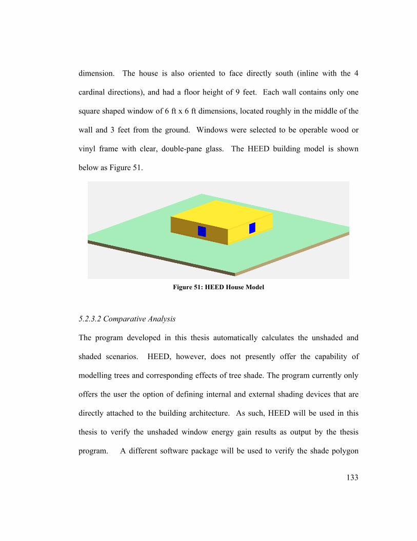
133
dimension. The house is also oriented to face directly south (inline with the 4
cardinal directions), and had a floor height of 9 feet. Each wall contains only one
square shaped window of 6 ft x 6 ft dimensions, located roughly in the middle of the
wall and 3 feet from the ground. Windows were selected to be operable wood or
vinyl frame with clear, double-pane glass. The HEED building model is shown
below as Figure 51.
Figure 51: HEED House Model
5.2.3.2 Comparative Analysis
The program developed in this thesis automatically calculates the unshaded and
shaded scenarios. HEED, however, does not presently offer the capability of
modelling trees and corresponding effects of tree shade. The program currently only
offers the user the option of defining internal and external shading devices that are
directly attached to the building architecture. As such, HEED will be used in this
thesis to verify the unshaded window energy gain results as output by the thesis
program. A different software package will be used to verify the shade polygon

134
projections and subsequent reductions in energy gain through the shaded
fenestration.
5.2.4 COMPARISON OF OUTPUTS FOR EAST WINDOW
Several tests were done to compare the results of the HEED simulations to the
program outputs. These results were used mainly for verification of energy gain
calculations through fenestration surfaces. The following section outlines the
procedure and presents the comparisons for the east window.
The HEED software offers several different methods of examining the heat gain
through fenestration surfaces. Firstly, the program provides three-dimensional plots
of the average value of the energy gain (in Btu/hr) through fenestration surfaces for
every hour of every day of the year. The user can select to view the window loads
for east facing, south facing, or west facing walls. Figure 52 below shows such a
plot for an east-facing window.
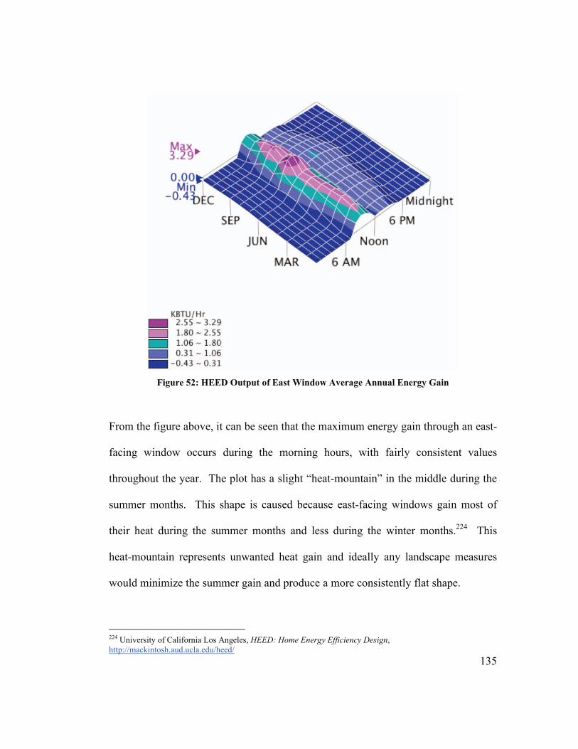
135
Figure 52: HEED Output of East Window Average Annual Energy Gain
From the figure above, it can be seen that the maximum energy gain through an east-
facing window occurs during the morning hours, with fairly consistent values
throughout the year. The plot has a slight “heat-mountain” in the middle during the
summer months. This shape is caused because east-facing windows gain most of
their heat during the summer months and less during the winter months.224 This
heat-mountain represents unwanted heat gain and ideally any landscape measures
would minimize the summer gain and produce a more consistently flat shape.
224 University of California Los Angeles, HEED: Home Energy Efficiency Design, http://mackintosh.aud.ucla.edu/heed/
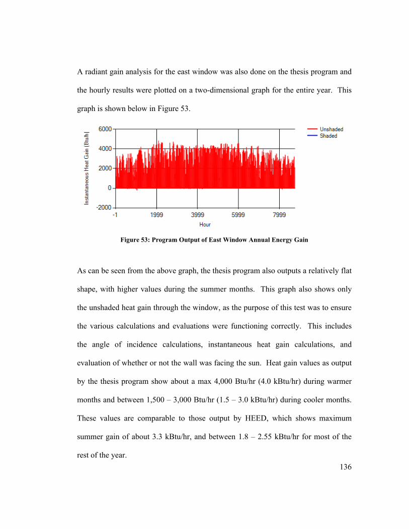
136
A radiant gain analysis for the east window was also done on the thesis program and
the hourly results were plotted on a two-dimensional graph for the entire year. This
graph is shown below in Figure 53.
Figure 53: Program Output of East Window Annual Energy Gain
As can be seen from the above graph, the thesis program also outputs a relatively flat
shape, with higher values during the summer months. This graph also shows only
the unshaded heat gain through the window, as the purpose of this test was to ensure
the various calculations and evaluations were functioning correctly. This includes
the angle of incidence calculations, instantaneous heat gain calculations, and
evaluation of whether or not the wall was facing the sun. Heat gain values as output
by the thesis program show about a max 4,000 Btu/hr (4.0 kBtu/hr) during warmer
months and between 1,500 – 3,000 Btu/hr (1.5 – 3.0 kBtu/hr) during cooler months.
These values are comparable to those output by HEED, which shows maximum
summer gain of about 3.3 kBtu/hr, and between 1.8 – 2.55 kBtu/hr for most of the
rest of the year.

137
HEED also offers the user the option of performing a twelve-day analysis, which
provides exact values for every hour of the day over the selected twelve day period.
Four separate twelve-day analyses were performed, one for each of the periods
around March 21, June 21, September 21, and December 21. Corresponding single
day analyses were performed in the thesis program by running the program for each
day using year hour values corresponding to that day. For example, the June 21st
single day test would perform the analysis between the hours of 4105 to 4128 (an
entire year consists of 8760 hours). Figure 54 and 55 below show a comparison of
the energy gain around March 21st. The HEED graph shows a twelve-day analysis
(ranging from March 16 – 27), while the thesis program graph shows only March 22.
It was originally planned to use the TMY3 data for March 21, however mid-day
values for March 21 were less than 5% of the mid-day values for the majority of
other days in March. Even though TMY3 data is statistical and not real (and so the
values for March 21 might be acceptable and consistent for that particular day), it
was decided to use an alternate day for data that had values that more resembled data
for the remaining days of March. Thus weather data for March 22 was used instead.
It is not possible to plot a single day graph in HEED, which is why the twelve-day
analysis is used here.
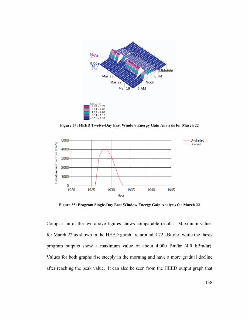
138
Figure 54: HEED Twelve-Day East Window Energy Gain Analysis for March 22
Figure 55: Program Single-Day East Window Energy Gain Analysis for March 22
Comparison of the two above figures shows comparable results. Maximum values
for March 22 as shown in the HEED graph are around 3.72 kBtu/hr, while the thesis
program outputs show a maximum value of about 4,000 Btu/hr (4.0 kBtu/hr).
Values for both graphs rise steeply in the morning and have a more gradual decline
after reaching the peak value. It can also be seen from the HEED output graph that
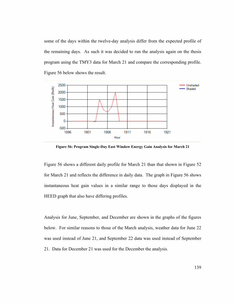
139
some of the days within the twelve-day analysis differ from the expected profile of
the remaining days. As such it was decided to run the analysis again on the thesis
program using the TMY3 data for March 21 and compare the corresponding profile.
Figure 56 below shows the result.
Figure 56: Program Single-Day East Window Energy Gain Analysis for March 21
Figure 56 shows a different daily profile for March 21 than that shown in Figure 52
for March 21 and reflects the difference in daily data. The graph in Figure 56 shows
instantaneous heat gain values in a similar range to those days displayed in the
HEED graph that also have differing profiles.
Analysis for June, September, and December are shown in the graphs of the figures
below. For similar reasons to those of the March analysis, weather data for June 22
was used instead of June 21, and September 22 data was used instead of September
21. Data for December 21 was used for the December the analysis.

140
Figure 57: HEED Twelve-Day East Window Energy Gain Analysis for June 22
Figure 58: Program Single-Day East Window Energy Gain Analysis for June 22

141
Figure 59: HEED Twelve-Day East Window Energy Gain Analysis for September 22
Figure 60: Program Single-Day East Window Energy Gain Analysis for September 22
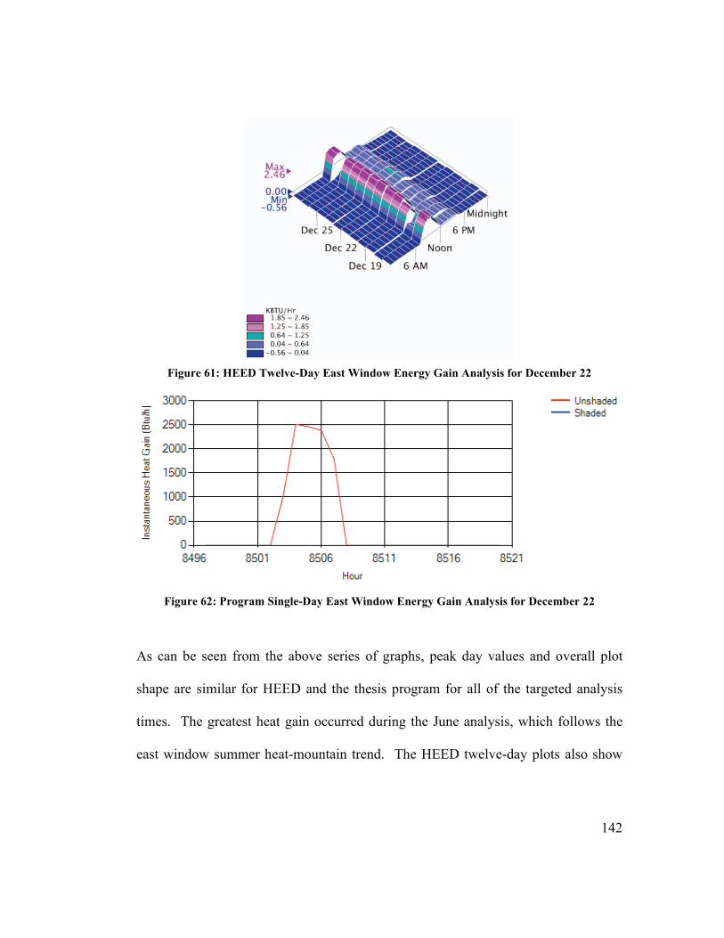
142
Figure 61: HEED Twelve-Day East Window Energy Gain Analysis for December 22
Figure 62: Program Single-Day East Window Energy Gain Analysis for December 22
As can be seen from the above series of graphs, peak day values and overall plot
shape are similar for HEED and the thesis program for all of the targeted analysis
times. The greatest heat gain occurred during the June analysis, which follows the
east window summer heat-mountain trend. The HEED twelve-day plots also show
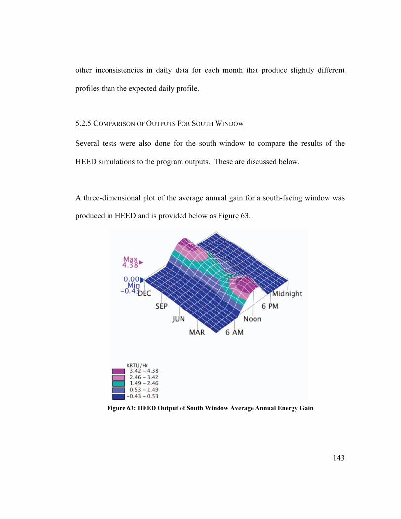
143
other inconsistencies in daily data for each month that produce slightly different
profiles than the expected daily profile.
5.2.5 COMPARISON OF OUTPUTS FOR SOUTH WINDOW
Several tests were also done for the south window to compare the results of the
HEED simulations to the program outputs. These are discussed below.
A three-dimensional plot of the average annual gain for a south-facing window was
produced in HEED and is provided below as Figure 63.
Figure 63: HEED Output of South Window Average Annual Energy Gain
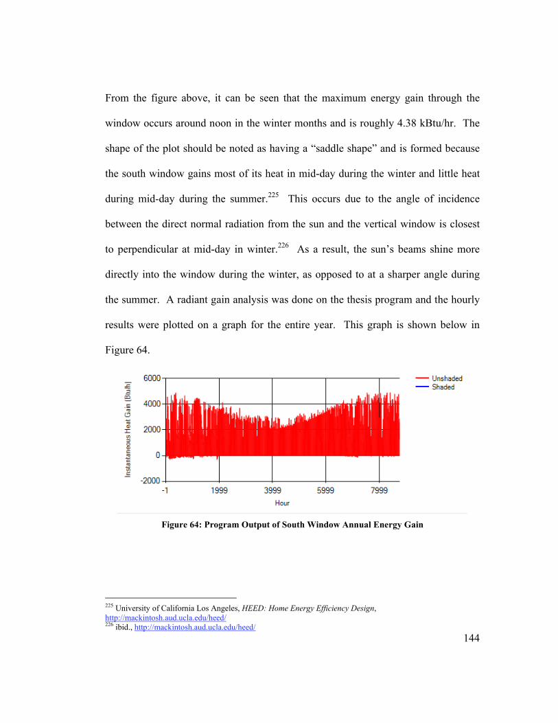
144
From the figure above, it can be seen that the maximum energy gain through the
window occurs around noon in the winter months and is roughly 4.38 kBtu/hr. The
shape of the plot should be noted as having a “saddle shape” and is formed because
the south window gains most of its heat in mid-day during the winter and little heat
during mid-day during the summer.225 This occurs due to the angle of incidence
between the direct normal radiation from the sun and the vertical window is closest
to perpendicular at mid-day in winter.226 As a result, the sun’s beams shine more
directly into the window during the winter, as opposed to at a sharper angle during
the summer. A radiant gain analysis was done on the thesis program and the hourly
results were plotted on a graph for the entire year. This graph is shown below in
Figure 64.
Figure 64: Program Output of South Window Annual Energy Gain
225 University of California Los Angeles, HEED: Home Energy Efficiency Design, http://mackintosh.aud.ucla.edu/heed/ 226 ibid., http://mackintosh.aud.ucla.edu/heed/
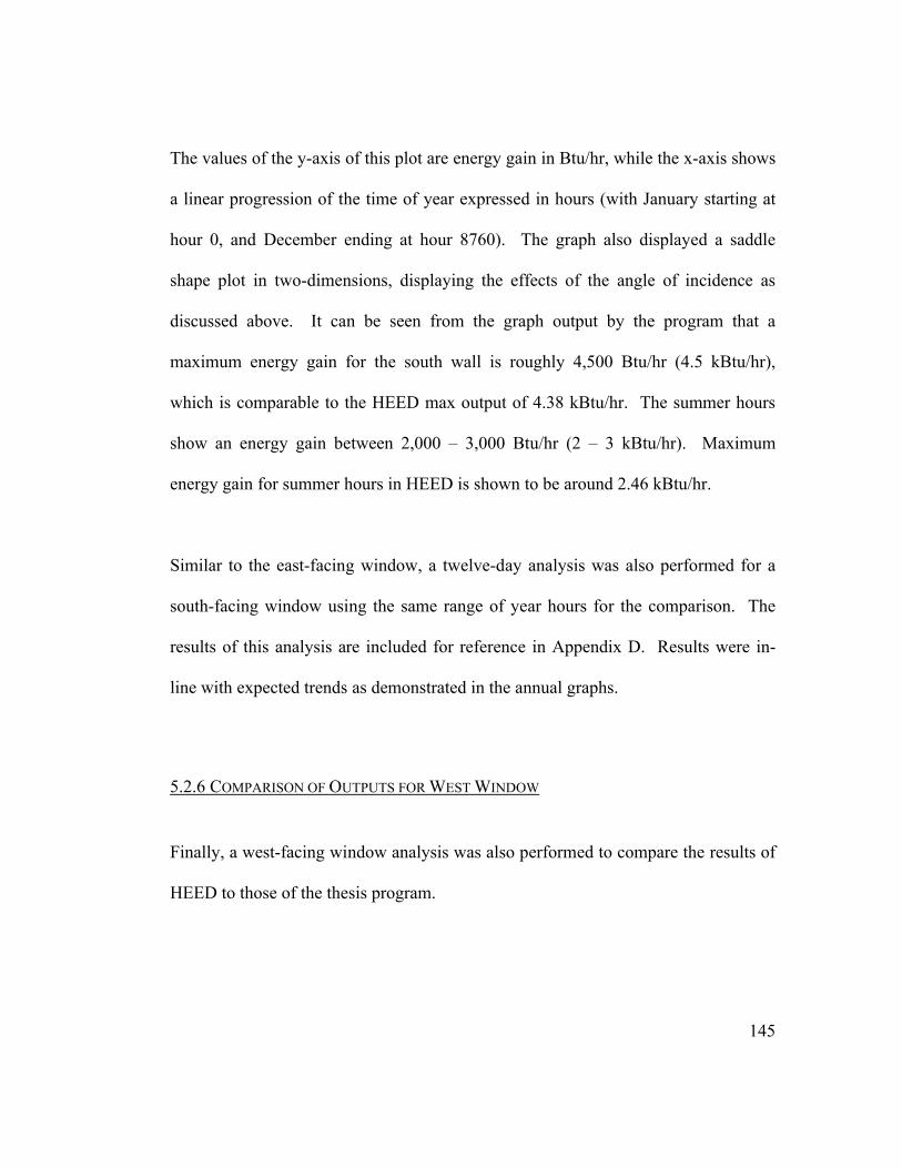
145
The values of the y-axis of this plot are energy gain in Btu/hr, while the x-axis shows
a linear progression of the time of year expressed in hours (with January starting at
hour 0, and December ending at hour 8760). The graph also displayed a saddle
shape plot in two-dimensions, displaying the effects of the angle of incidence as
discussed above. It can be seen from the graph output by the program that a
maximum energy gain for the south wall is roughly 4,500 Btu/hr (4.5 kBtu/hr),
which is comparable to the HEED max output of 4.38 kBtu/hr. The summer hours
show an energy gain between 2,000 – 3,000 Btu/hr (2 – 3 kBtu/hr). Maximum
energy gain for summer hours in HEED is shown to be around 2.46 kBtu/hr.
Similar to the east-facing window, a twelve-day analysis was also performed for a
south-facing window using the same range of year hours for the comparison. The
results of this analysis are included for reference in Appendix D. Results were in-
line with expected trends as demonstrated in the annual graphs.
5.2.6 COMPARISON OF OUTPUTS FOR WEST WINDOW
Finally, a west-facing window analysis was also performed to compare the results of
HEED to those of the thesis program.
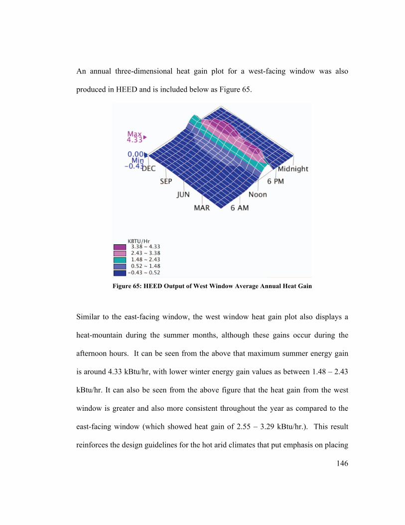
146
An annual three-dimensional heat gain plot for a west-facing window was also
produced in HEED and is included below as Figure 65.
Figure 65: HEED Output of West Window Average Annual Heat Gain
Similar to the east-facing window, the west window heat gain plot also displays a
heat-mountain during the summer months, although these gains occur during the
afternoon hours. It can be seen from the above that maximum summer energy gain
is around 4.33 kBtu/hr, with lower winter energy gain values as between 1.48 – 2.43
kBtu/hr. It can also be seen from the above figure that the heat gain from the west
window is greater and also more consistent throughout the year as compared to the
east-facing window (which showed heat gain of 2.55 – 3.29 kBtu/hr.). This result
reinforces the design guidelines for the hot arid climates that put emphasis on placing
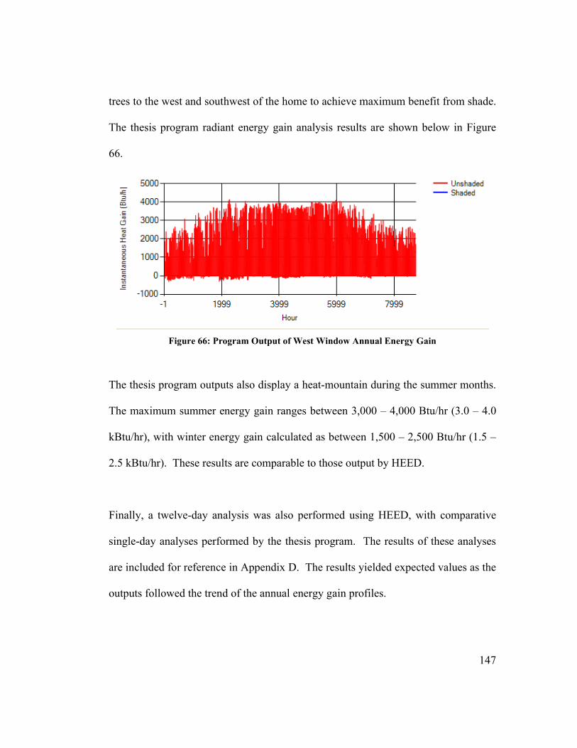
147
trees to the west and southwest of the home to achieve maximum benefit from shade.
The thesis program radiant energy gain analysis results are shown below in Figure
66.
Figure 66: Program Output of West Window Annual Energy Gain
The thesis program outputs also display a heat-mountain during the summer months.
The maximum summer energy gain ranges between 3,000 – 4,000 Btu/hr (3.0 – 4.0
kBtu/hr), with winter energy gain calculated as between 1,500 – 2,500 Btu/hr (1.5 –
2.5 kBtu/hr). These results are comparable to those output by HEED.
Finally, a twelve-day analysis was also performed using HEED, with comparative
single-day analyses performed by the thesis program. The results of these analyses
are included for reference in Appendix D. The results yielded expected values as the
outputs followed the trend of the annual energy gain profiles.
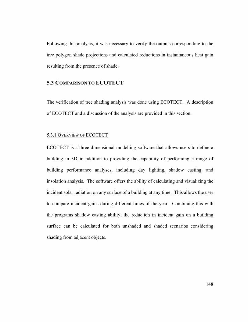
148
Following this analysis, it was necessary to verify the outputs corresponding to the
tree polygon shade projections and calculated reductions in instantaneous heat gain
resulting from the presence of shade.
5.3 COMPARISON TO ECOTECT
The verification of tree shading analysis was done using ECOTECT. A description
of ECOTECT and a discussion of the analysis are provided in this section.
5.3.1 OVERVIEW OF ECOTECT
ECOTECT is a three-dimensional modelling software that allows users to define a
building in 3D in addition to providing the capability of performing a range of
building performance analyses, including day lighting, shadow casting, and
insolation analysis. The software offers the ability of calculating and visualizing the
incident solar radiation on any surface of a building at any time. This allows the user
to compare incident gains during different times of the year. Combining this with
the programs shadow casting ability, the reduction in incident gain on a building
surface can be calculated for both unshaded and shaded scenarios considering
shading from adjacent objects.
149
5.3.1.1 Shading Analysis in ECOTECT
ECOTECT offers the user the capability of viewing the three-dimensional model
from the perspective of the sun at its position in the sky. The software enables this
view by constructing accurate sun-path diagrams from uploaded weather data. A
specific date can be selected to construct a daily sun path diagram. An example of
such a sun path diagram is shown below in Figure 67.
Figure 67: Example ECOTECT Model with Sun-Path Diagram
The time of day can also be selected, and the corresponding view of the model from
that specific sun position can be observed. Figure 68 below shows the sun position
at 11:00 am on November 21.
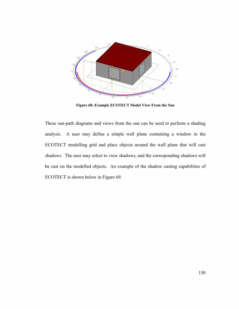
150
Figure 68: Example ECOTECT Model View From the Sun
These sun-path diagrams and views from the sun can be used to perform a shading
analysis. A user may define a simple wall plane containing a window in the
ECOTECT modelling grid and place objects around the wall plane that will cast
shadows. The user may select to view shadows, and the corresponding shadows will
be cast on the modelled objects. An example of the shadow casting capabilities of
ECOTECT is shown below in Figure 69.
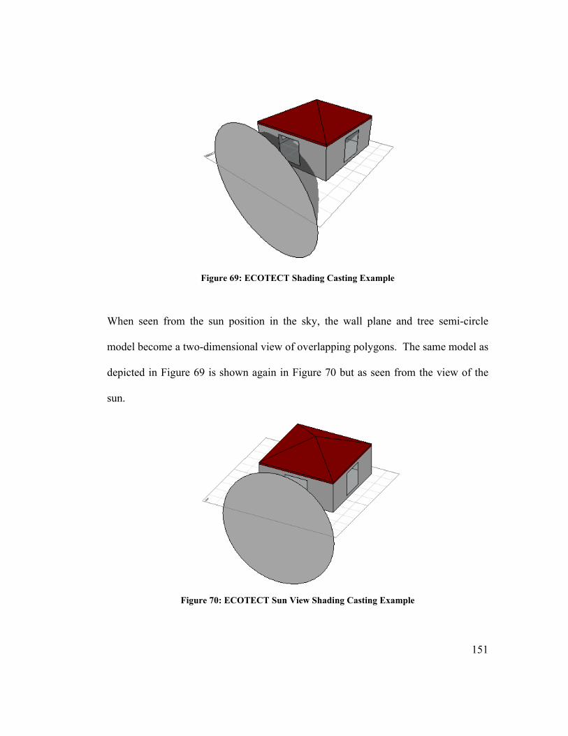
151
Figure 69: ECOTECT Shading Casting Example
When seen from the sun position in the sky, the wall plane and tree semi-circle
model become a two-dimensional view of overlapping polygons. The same model as
depicted in Figure 69 is shown again in Figure 70 but as seen from the view of the
sun.
Figure 70: ECOTECT Sun View Shading Casting Example
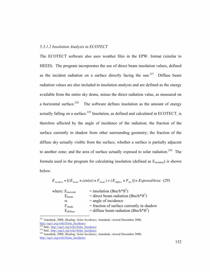
152
5.3.1.2 Insolation Analysis in ECOTECT
The ECOTECT software also uses weather files in the EPW. format (similar to
HEED). The program incorporates the use of direct beam insolation values, defined
as the incident radiation on a surface directly facing the sun.227 Diffuse beam
radiation values are also included in insolation analysis and are defined as the energy
available from the entire sky dome, minus the direct radiation value, as measured on
a horizontal surface.228 The software defines insolation as the amount of energy
actually falling on a surface.229 Insolation, as defined and calculated in ECOTECT, is
therefore affected by the angle of incidence of the radiation; the fraction of the
surface currently in shadow from other surrounding geometry; the fraction of the
diffuse sky actually visible from the surface; whether a surface is partially adjacent
to another zone; and the area of surface actually exposed to solar radiation.230 The
formula used in the program for calculating insolation (defined as Eincident) is shown
below:
Eincident = [(Ebeam cos( ) Fshade ) + (Ediffuse Fsky )] ExposedArea (29)
where: Eincicent = insolation (Btu/h*ft2) Ebeam = direct beam radiation (Btu/h*ft2) = angle of incidence
Fshade = fraction of surface currently in shadow Ediffuse = diffuse beam radiation (Btu/h*ft2)
227 Autodesk, 2008, Shading: Solar Incidence, Autodesk, viewed December 2008, http://squ1.org/wiki/Solar_Incidence 228 ibid., http://squ1.org/wiki/Solar_Incidence 229 ibid., http://squ1.org/wiki/Solar_Incidence 230 Autodesk, 2008, Shading: Solar Incidence, Autodesk, viewed December 2008, http://squ1.org/wiki/Solar_Incidence
153
Fsky = fraction of diffuse sky visible from the surface Exposed Area = area of building surface to be analyzed (ft2)
ECOTECT also uses separate calculations to determine the amount of absorbed and
transmitted radiation, depending on the type of surface being analyzed. The software
then offers the user the ability to perform hourly, monthly, or annual insolation
analysis for specified surfaces. Ground reflection can be eliminated from the
analysis in order to isolate the direct beam incident solar radiation gains into the
building.
5.3.2 THESIS PROGRAM AND ECOTECT INPUTS
Similar to the HEED analysis, buildings and fenestration surfaces were constructed
in order to verify and compare the outputs of the thesis program versus those of
ECOTECT.
5.3.2.1 Building Definition in ECOTECT – Dimensions and Fenestration
Since several different tests were performed using ECOTECT, different building
definitions were constructed based on the analysis. Simple wall planes were
constructed for the matrix transformation and shading analysis while a single zone,
one-story building was constructed for the insolation analysis. The single wall
planes were defined with a 20-foot length and 9-foot height. A window of 6 ft x 6 ft
dimension was placed in the middle of the wall, at a sill height of 2 feet. For the
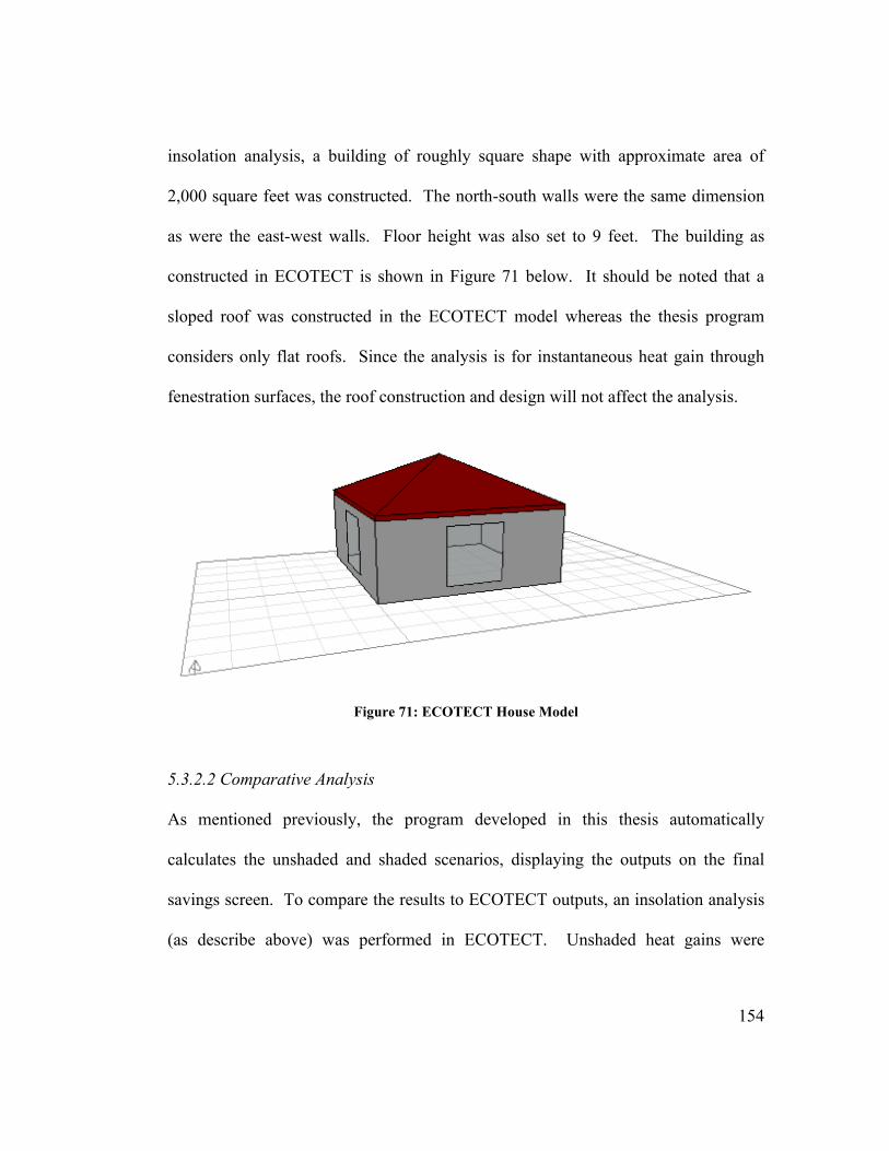
154
insolation analysis, a building of roughly square shape with approximate area of
2,000 square feet was constructed. The north-south walls were the same dimension
as were the east-west walls. Floor height was also set to 9 feet. The building as
constructed in ECOTECT is shown in Figure 71 below. It should be noted that a
sloped roof was constructed in the ECOTECT model whereas the thesis program
considers only flat roofs. Since the analysis is for instantaneous heat gain through
fenestration surfaces, the roof construction and design will not affect the analysis.
Figure 71: ECOTECT House Model
5.3.2.2 Comparative Analysis
As mentioned previously, the program developed in this thesis automatically
calculates the unshaded and shaded scenarios, displaying the outputs on the final
savings screen. To compare the results to ECOTECT outputs, an insolation analysis
(as describe above) was performed in ECOTECT. Unshaded heat gains were
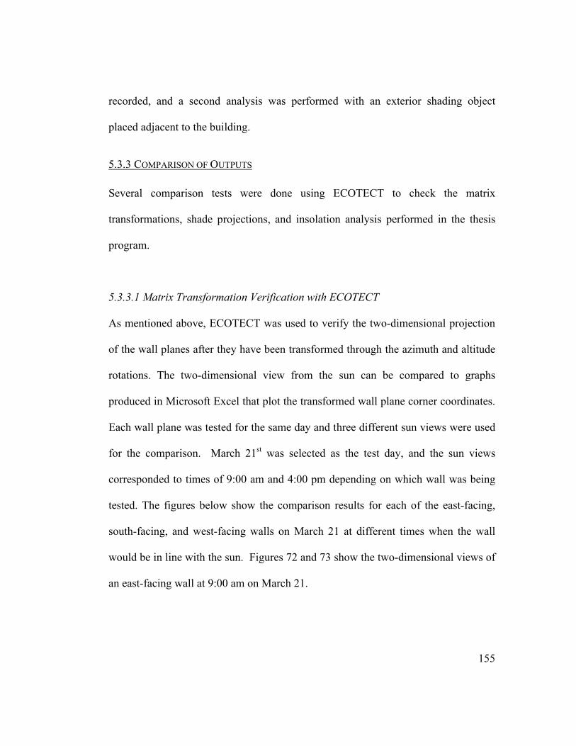
155
recorded, and a second analysis was performed with an exterior shading object
placed adjacent to the building.
5.3.3 COMPARISON OF OUTPUTS
Several comparison tests were done using ECOTECT to check the matrix
transformations, shade projections, and insolation analysis performed in the thesis
program.
5.3.3.1 Matrix Transformation Verification with ECOTECT
As mentioned above, ECOTECT was used to verify the two-dimensional projection
of the wall planes after they have been transformed through the azimuth and altitude
rotations. The two-dimensional view from the sun can be compared to graphs
produced in Microsoft Excel that plot the transformed wall plane corner coordinates.
Each wall plane was tested for the same day and three different sun views were used
for the comparison. March 21st was selected as the test day, and the sun views
corresponded to times of 9:00 am and 4:00 pm depending on which wall was being
tested. The figures below show the comparison results for each of the east-facing,
south-facing, and west-facing walls on March 21 at different times when the wall
would be in line with the sun. Figures 72 and 73 show the two-dimensional views of
an east-facing wall at 9:00 am on March 21.

156
Figure 72: Excel Sun View of East-Facing
Wall at 9:00 am
Figure 73: ECOTECT Sun View of East-Facing Wall
at 9:00 am
Figures 74 to 77 show a south-facing wall on March 21 at 9:00 am and 4:00 pm.
Figure 74: Excel Sun View of South-Facing Wall at
9:00 am
Figure 75: ECOTECT Sun View of South-
Facing Wall at 9:00 am
Figure 76: Excel Sun View of South-Facing Wall at
4:00 pm
Figure 77: ECOTECT Sun View of South-
Facing Wall at 4:00 pm
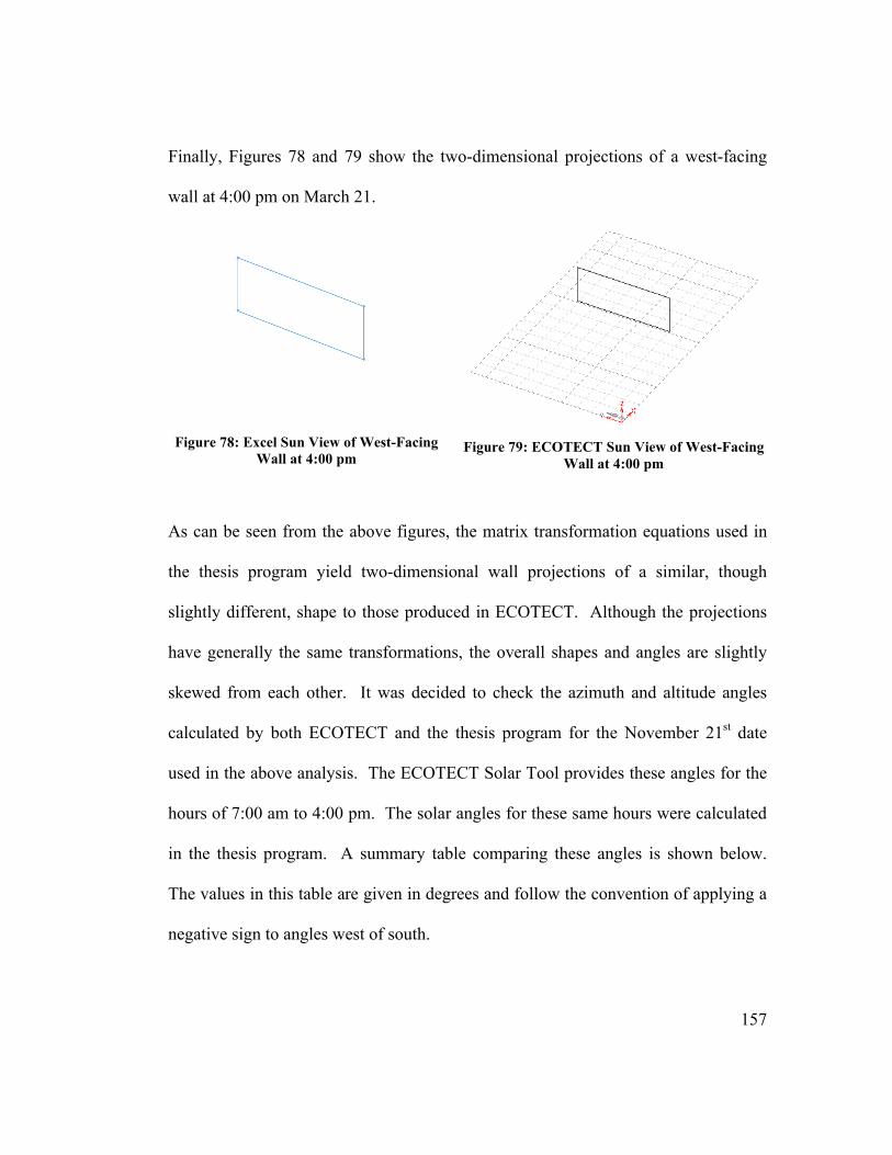
157
Finally, Figures 78 and 79 show the two-dimensional projections of a west-facing
wall at 4:00 pm on March 21.
Figure 78: Excel Sun View of West-Facing
Wall at 4:00 pm
Figure 79: ECOTECT Sun View of West-Facing
Wall at 4:00 pm
As can be seen from the above figures, the matrix transformation equations used in
the thesis program yield two-dimensional wall projections of a similar, though
slightly different, shape to those produced in ECOTECT. Although the projections
have generally the same transformations, the overall shapes and angles are slightly
skewed from each other. It was decided to check the azimuth and altitude angles
calculated by both ECOTECT and the thesis program for the November 21st date
used in the above analysis. The ECOTECT Solar Tool provides these angles for the
hours of 7:00 am to 4:00 pm. The solar angles for these same hours were calculated
in the thesis program. A summary table comparing these angles is shown below.
The values in this table are given in degrees and follow the convention of applying a
negative sign to angles west of south.
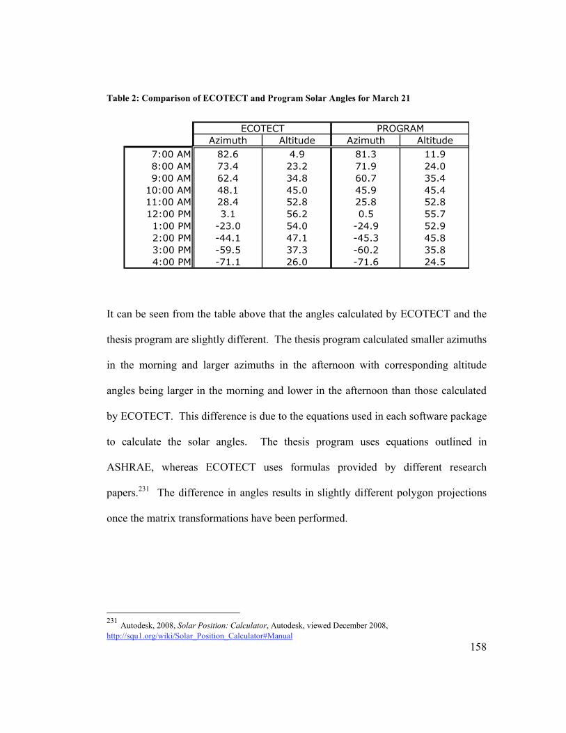
158
Table 2: Comparison of ECOTECT and Program Solar Angles for March 21
It can be seen from the table above that the angles calculated by ECOTECT and the
thesis program are slightly different. The thesis program calculated smaller azimuths
in the morning and larger azimuths in the afternoon with corresponding altitude
angles being larger in the morning and lower in the afternoon than those calculated
by ECOTECT. This difference is due to the equations used in each software package
to calculate the solar angles. The thesis program uses equations outlined in
ASHRAE, whereas ECOTECT uses formulas provided by different research
papers.231 The difference in angles results in slightly different polygon projections
once the matrix transformations have been performed.
231 Autodesk, 2008, Solar Position: Calculator, Autodesk, viewed December 2008,
http://squ1.org/wiki/Solar_Position_Calculator#Manual
Azimuth Altitude Azimuth Altitude
7:00 AM 82.6 4.9 81.3 11.9
8:00 AM 73.4 23.2 71.9 24.0
9:00 AM 62.4 34.8 60.7 35.4
10:00 AM 48.1 45.0 45.9 45.4
11:00 AM 28.4 52.8 25.8 52.8
12:00 PM 3.1 56.2 0.5 55.7
1:00 PM -23.0 54.0 -24.9 52.9
2:00 PM -44.1 47.1 -45.3 45.8
3:00 PM -59.5 37.3 -60.2 35.8
4:00 PM -71.1 26.0 -71.6 24.5
ECOTECT PROGRAM
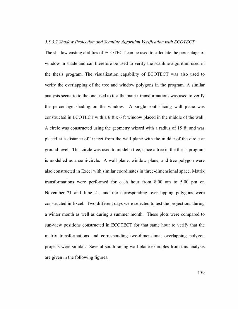
159
5.3.3.2 Shadow Projection and Scanline Algorithm Verification with ECOTECT
The shadow casting abilities of ECOTECT can be used to calculate the percentage of
window in shade and can therefore be used to verify the scanline algorithm used in
the thesis program. The visualization capability of ECOTECT was also used to
verify the overlapping of the tree and window polygons in the program. A similar
analysis scenario to the one used to test the matrix transformations was used to verify
the percentage shading on the window. A single south-facing wall plane was
constructed in ECOTECT with a 6 ft x 6 ft window placed in the middle of the wall.
A circle was constructed using the geometry wizard with a radius of 15 ft, and was
placed at a distance of 10 feet from the wall plane with the middle of the circle at
ground level. This circle was used to model a tree, since a tree in the thesis program
is modelled as a semi-circle. A wall plane, window plane, and tree polygon were
also constructed in Excel with similar coordinates in three-dimensional space. Matrix
transformations were performed for each hour from 8:00 am to 5:00 pm on
November 21 and June 21, and the corresponding over-lapping polygons were
constructed in Excel. Two different days were selected to test the projections during
a winter month as well as during a summer month. These plots were compared to
sun-view positions constructed in ECOTECT for that same hour to verify that the
matrix transformations and corresponding two-dimensional overlapping polygon
projects were similar. Several south-racing wall plane examples from this analysis
are given in the following figures.
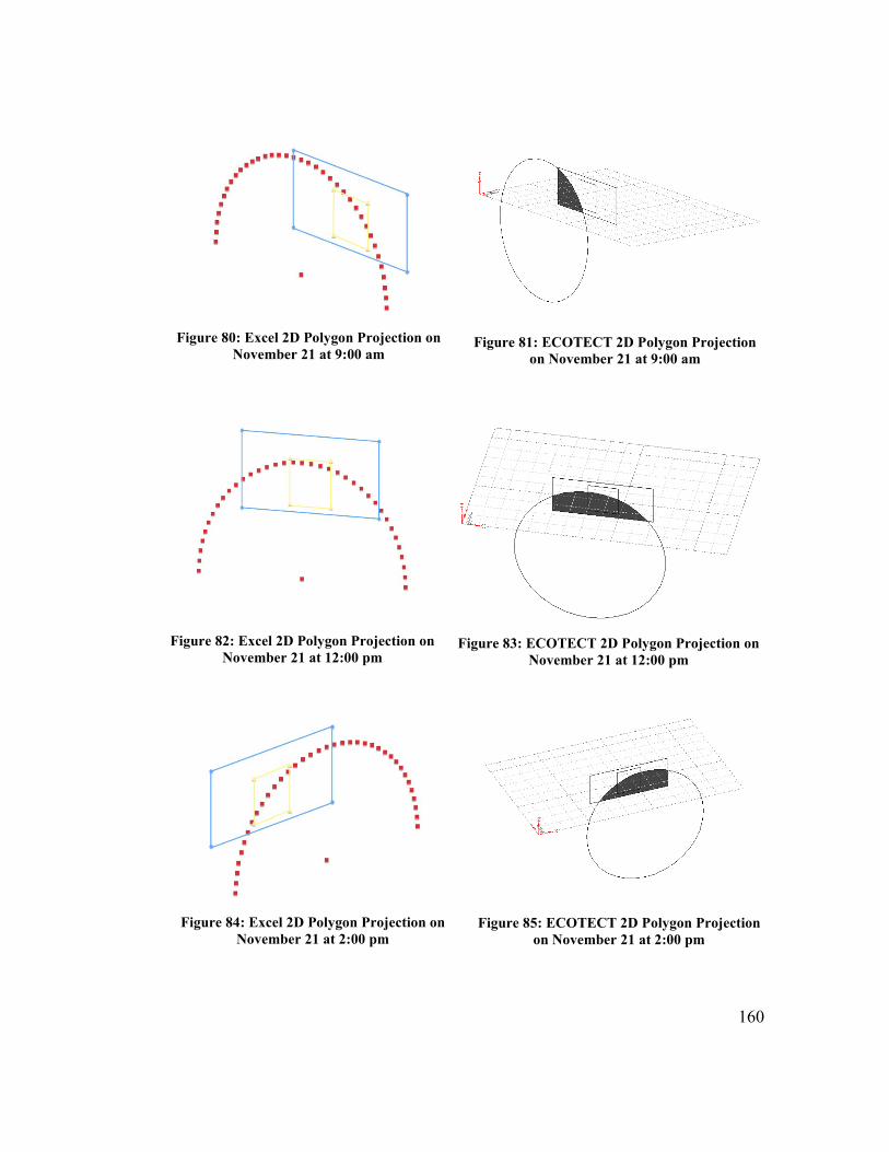
160
Figure 80: Excel 2D Polygon Projection on
November 21 at 9:00 am
Figure 81: ECOTECT 2D Polygon Projection
on November 21 at 9:00 am
Figure 82: Excel 2D Polygon Projection on
November 21 at 12:00 pm
Figure 83: ECOTECT 2D Polygon Projection on
November 21 at 12:00 pm
Figure 84: Excel 2D Polygon Projection on
November 21 at 2:00 pm
Figure 85: ECOTECT 2D Polygon Projection
on November 21 at 2:00 pm
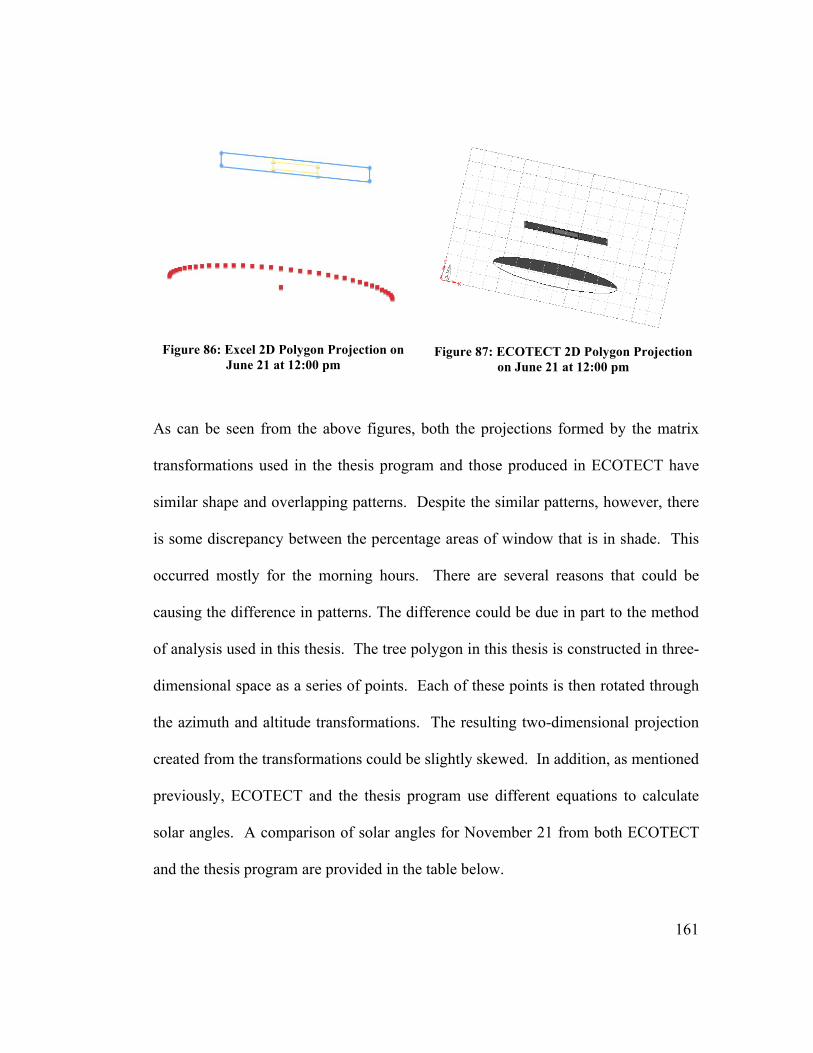
161
Figure 86: Excel 2D Polygon Projection on
June 21 at 12:00 pm
Figure 87: ECOTECT 2D Polygon Projection
on June 21 at 12:00 pm
As can be seen from the above figures, both the projections formed by the matrix
transformations used in the thesis program and those produced in ECOTECT have
similar shape and overlapping patterns. Despite the similar patterns, however, there
is some discrepancy between the percentage areas of window that is in shade. This
occurred mostly for the morning hours. There are several reasons that could be
causing the difference in patterns. The difference could be due in part to the method
of analysis used in this thesis. The tree polygon in this thesis is constructed in three-
dimensional space as a series of points. Each of these points is then rotated through
the azimuth and altitude transformations. The resulting two-dimensional projection
created from the transformations could be slightly skewed. In addition, as mentioned
previously, ECOTECT and the thesis program use different equations to calculate
solar angles. A comparison of solar angles for November 21 from both ECOTECT
and the thesis program are provided in the table below.
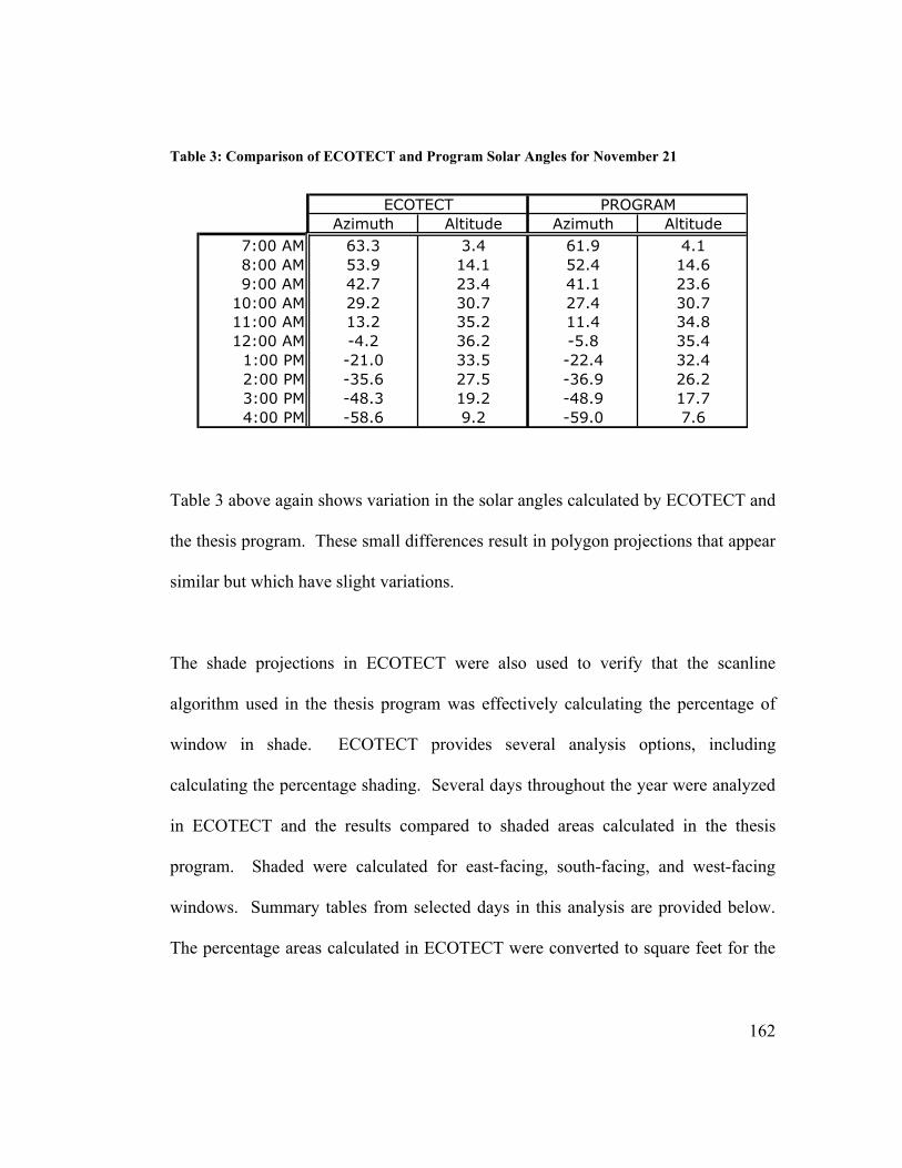
162
Table 3: Comparison of ECOTECT and Program Solar Angles for November 21
Table 3 above again shows variation in the solar angles calculated by ECOTECT and
the thesis program. These small differences result in polygon projections that appear
similar but which have slight variations.
The shade projections in ECOTECT were also used to verify that the scanline
algorithm used in the thesis program was effectively calculating the percentage of
window in shade. ECOTECT provides several analysis options, including
calculating the percentage shading. Several days throughout the year were analyzed
in ECOTECT and the results compared to shaded areas calculated in the thesis
program. Shaded were calculated for east-facing, south-facing, and west-facing
windows. Summary tables from selected days in this analysis are provided below.
The percentage areas calculated in ECOTECT were converted to square feet for the
Azimuth Altitude Azimuth Altitude
7:00 AM 63.3 3.4 61.9 4.1
8:00 AM 53.9 14.1 52.4 14.6
9:00 AM 42.7 23.4 41.1 23.6
10:00 AM 29.2 30.7 27.4 30.7
11:00 AM 13.2 35.2 11.4 34.8
12:00 AM -4.2 36.2 -5.8 35.4
1:00 PM -21.0 33.5 -22.4 32.4
2:00 PM -35.6 27.5 -36.9 26.2
3:00 PM -48.3 19.2 -48.9 17.7
4:00 PM -58.6 9.2 -59.0 7.6
ECOTECT PROGRAM

163
purpose of this analysis since the thesis program provides outputs in units of square
feet. The example days are February 21, June 21, and November 21.
Table 4: ECOTECT vs Program Shaded Areas for East Wall
Table 5: ECOTECT vs Program Shaded Areas South Wall
ECOTECT PROGRAM ECOTECT PROGRAM ECOTECT PROGRAM
Area (ft2) Area (ft2) Area (ft2) Area (ft2) Area (ft2) Area (ft2)
8:00 AM 36.0 28.8 36.0 29.0 36.0 22.4
9:00 AM 36.0 18.2 36.0 23.2 34.9 17.7
10:00 AM 20.9 1.3 24.1 3.3 9.7 4.1
11:00 AM 0.0 0.0 0.0 3.3 0.0 0.0
12:00 PM 0.0 0.0 0.0 0.0 0.0 0.0
1:00 PM 0.0 0.0 0.0 0.0 0.0 0.0
2:00 PM 0.0 0.0 0.0 0.0 0.0 0.0
3:00 PM 0.0 0.0 0.0 0.0 0.0 0.0
4:00 PM 0.0 0.0 0.0 0.0 0.0 0.0
February 21 June 21 November 21
ECOTECT PROGRAM ECOTECT PROGRAM ECOTECT PROGRAM
Area (ft2) Area (ft2) Area (ft2) Area (ft2) Area (ft2) Area (ft2)
8:00 AM 0.0 0.0 0.0 0.0 0.0 15.1
9:00 AM 0.0 10.9 0.0 0.0 5.8 22.0
10:00 AM 0.7 20.8 0.0 0.0 16.2 23.4
11:00 AM 4.0 16.7 0.0 0.0 20.9 28.6
12:00 PM 11.5 10.3 0.0 0.0 24.1 24.7
1:00 PM 10.4 13.3 0.0 0.0 25.9 26.5
2:00 PM 16.2 14.0 0.0 0.0 27.4 25.6
3:00 PM 9.7 8.0 0.0 0.0 22.7 21.7
4:00 PM 3.2 4.4 0.0 0.0 19.4 14.0
February 21 June 21 November 21
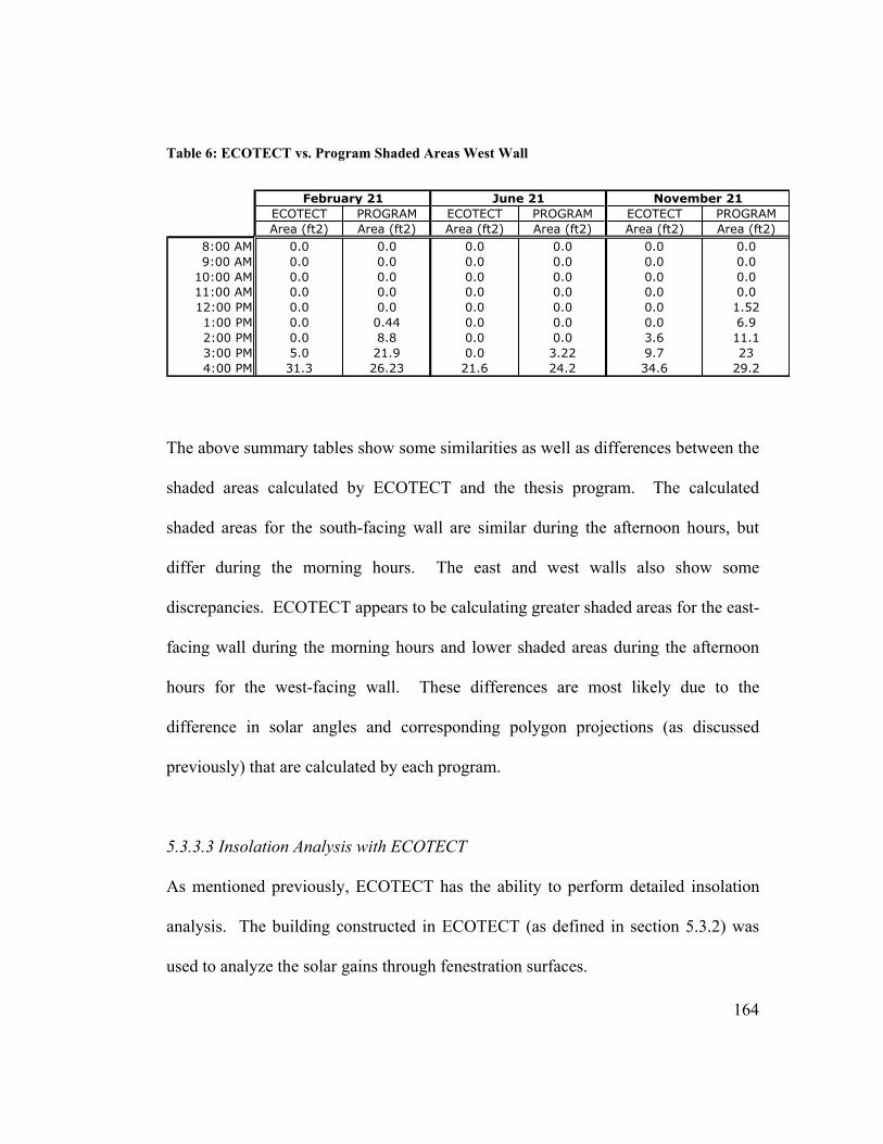
164
Table 6: ECOTECT vs. Program Shaded Areas West Wall
The above summary tables show some similarities as well as differences between the
shaded areas calculated by ECOTECT and the thesis program. The calculated
shaded areas for the south-facing wall are similar during the afternoon hours, but
differ during the morning hours. The east and west walls also show some
discrepancies. ECOTECT appears to be calculating greater shaded areas for the east-
facing wall during the morning hours and lower shaded areas during the afternoon
hours for the west-facing wall. These differences are most likely due to the
difference in solar angles and corresponding polygon projections (as discussed
previously) that are calculated by each program.
5.3.3.3 Insolation Analysis with ECOTECT
As mentioned previously, ECOTECT has the ability to perform detailed insolation
analysis. The building constructed in ECOTECT (as defined in section 5.3.2) was
used to analyze the solar gains through fenestration surfaces.
ECOTECT PROGRAM ECOTECT PROGRAM ECOTECT PROGRAM
Area (ft2) Area (ft2) Area (ft2) Area (ft2) Area (ft2) Area (ft2)
8:00 AM 0.0 0.0 0.0 0.0 0.0 0.0
9:00 AM 0.0 0.0 0.0 0.0 0.0 0.0
10:00 AM 0.0 0.0 0.0 0.0 0.0 0.0
11:00 AM 0.0 0.0 0.0 0.0 0.0 0.0
12:00 PM 0.0 0.0 0.0 0.0 0.0 1.52
1:00 PM 0.0 0.44 0.0 0.0 0.0 6.9
2:00 PM 0.0 8.8 0.0 0.0 3.6 11.1
3:00 PM 5.0 21.9 0.0 3.22 9.7 23
4:00 PM 31.3 26.23 21.6 24.2 34.6 29.2
February 21 June 21 November 21
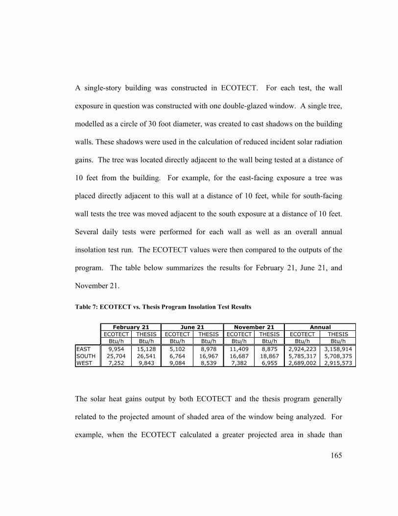
165
A single-story building was constructed in ECOTECT. For each test, the wall
exposure in question was constructed with one double-glazed window. A single tree,
modelled as a circle of 30 foot diameter, was created to cast shadows on the building
walls. These shadows were used in the calculation of reduced incident solar radiation
gains. The tree was located directly adjacent to the wall being tested at a distance of
10 feet from the building. For example, for the east-facing exposure a tree was
placed directly adjacent to this wall at a distance of 10 feet, while for south-facing
wall tests the tree was moved adjacent to the south exposure at a distance of 10 feet.
Several daily tests were performed for each wall as well as an overall annual
insolation test run. The ECOTECT values were then compared to the outputs of the
program. The table below summarizes the results for February 21, June 21, and
November 21.
Table 7: ECOTECT vs. Thesis Program Insolation Test Results
The solar heat gains output by both ECOTECT and the thesis program generally
related to the projected amount of shaded area of the window being analyzed. For
example, when the ECOTECT calculated a greater projected area in shade than
ECOTECT THESIS ECOTECT THESIS ECOTECT THESIS ECOTECT THESIS
Btu/h Btu/h Btu/h Btu/h Btu/h Btu/h Btu/h Btu/h
EAST 9,954 15,128 5,102 8,978 11,409 8,875 2,924,223 3,158,914
SOUTH 25,704 26,541 6,764 16,967 16,687 18,867 5,785,317 5,708,375
WEST 7,252 9,843 9,084 8,539 7,382 6,955 2,689,002 2,915,573
February 21 June 21 November 21 Annual

166
predicted by the thesis program, the heat gain was typically less than that output by
the program. Conversely, when ECOTECT calculated a smaller projected shaded
area than the thesis program, the corresponding solar gains were typically greater
than those output by the thesis program. The values output by ECOTECT and the
thesis program were also generally in the same range, within a difference of a few
kBtu//h. There were, however, several exceptions to the expected trends, which
could have occurred due to inconsistencies in weather data used in the calculations.
Despite these inconsistencies, the overall annual solar heat gains as calculated by
ECOTECT and the thesis program were within close range.
As can be seen from Table 7 above, the ECOTECT insolation analyses are
comparable to the test runs output by the thesis program. It can thus be concluded
that the thesis program is producing acceptable results based on comparisons to
industry standard software.
167
CHAPTER 6
The following chapter includes several comparisons to previous research
publications and presents final conclusions regarding the performance and
capabilities of the program developed in this thesis.
6.1 COMPARISON TO PREVIOUS RESEARCH PUBLICATIONS
As outlined in Chapter 2, several publications have been produced demonstrating the
range of savings that can be achieved through the use of microclimatic landscape
design. Selected results are discussed below. The program variables were input to
reproduce as closely as possible the scenarios outlined in the research. The results of
the research publications were then contrasted with those of the program.
6.1.1 PREVIOUS RESEARCH COMPARISON 1
A study published by McPherson evaluated the cost-effectiveness of shade trees for
demand side management.232 A single tree was placed opposite of the west wall of a
1,761 square foot residence. The tree was assumed to reach 24 ft in height at
maturity, and was assumed to obstruct 85% of incident solar radiation during its in-
leaf period and 25% during its leaf-off period. The scenario was tested for several
232 McPherson, EG, Evaluating the Cost Effectiveness of Shade Trees for Demand Side Management, The
Electricity Journal, vol. 6, no. 9, November, pp 57-65
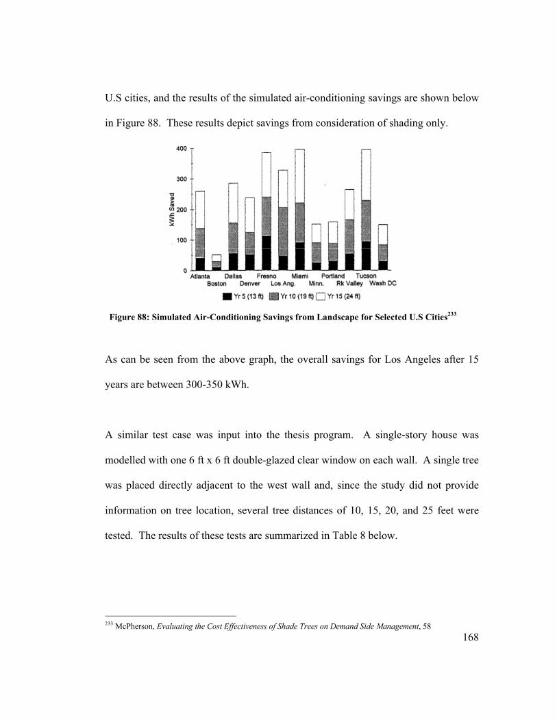
168
U.S cities, and the results of the simulated air-conditioning savings are shown below
in Figure 88. These results depict savings from consideration of shading only.
Figure 88: Simulated Air-Conditioning Savings from Landscape for Selected U.S Cities233
As can be seen from the above graph, the overall savings for Los Angeles after 15
years are between 300-350 kWh.
A similar test case was input into the thesis program. A single-story house was
modelled with one 6 ft x 6 ft double-glazed clear window on each wall. A single tree
was placed directly adjacent to the west wall and, since the study did not provide
information on tree location, several tree distances of 10, 15, 20, and 25 feet were
tested. The results of these tests are summarized in Table 8 below.
233 McPherson, Evaluating the Cost Effectiveness of Shade Trees on Demand Side Management, 58
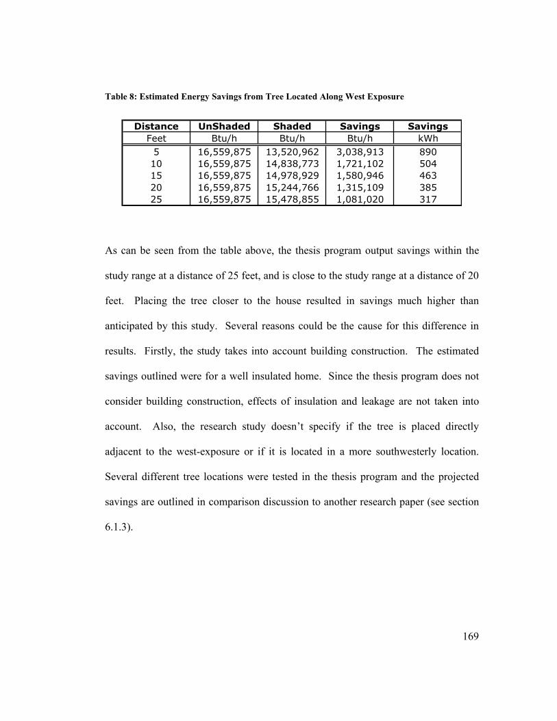
169
Table 8: Estimated Energy Savings from Tree Located Along West Exposure
As can be seen from the table above, the thesis program output savings within the
study range at a distance of 25 feet, and is close to the study range at a distance of 20
feet. Placing the tree closer to the house resulted in savings much higher than
anticipated by this study. Several reasons could be the cause for this difference in
results. Firstly, the study takes into account building construction. The estimated
savings outlined were for a well insulated home. Since the thesis program does not
consider building construction, effects of insulation and leakage are not taken into
account. Also, the research study doesn’t specify if the tree is placed directly
adjacent to the west-exposure or if it is located in a more southwesterly location.
Several different tree locations were tested in the thesis program and the projected
savings are outlined in comparison discussion to another research paper (see section
6.1.3).
Distance UnShaded Shaded Savings Savings
Feet Btu/h Btu/h Btu/h kWh
5 16,559,875 13,520,962 3,038,913 890
10 16,559,875 14,838,773 1,721,102 504
15 16,559,875 14,978,929 1,580,946 463
20 16,559,875 15,244,766 1,315,109 385
25 16,559,875 15,478,855 1,081,020 317
170
6.1.2 PREVIOUS RESEARCH COMPARISON 2
A study published by Simpson and McPherson investigated the potential of tree
shade for reducing residential energy use in California.234 The study used a
computer simulation package known as the Shadow Pattern Simulator (SPS) to
calculate the shade on buildings for various tree configurations. The SPS calculates
hourly tree shade for each wall surface based on building and tree sizes and their
relative orientations and distances from buildings.235 The shade patterns were
transferred to another software package, MICROPAS, to perform the building
simulations.236 Trees in the study were modelled to be 25 ft tall at maturity, with
equal canopy diameter, and were simulated as blocking 85% of incoming solar
radiation when in leaf and 30% during off-leaf periods. The standard base case
building was a single story frame house of 1,500 square feet, oriented along the
cardinal directions with windows evenly distributed along each wall.237 The impact
of single trees planted adjacent to east, south, and west walls as well as at building
corners were simulated.
The results of this study found that the annual savings due to a 24-foot tall tree
placed to the west of the building were about 12%.238 A similar scenario was tested
in the thesis program. Since the study does not provide information on the distance
234 McPherson et al., Potential of Tree Shade for Reducing Residential Energy Use in California, 11 235 ibid., 11 236 ibid., 11 237 ibid., 12 238 ibid., 13

171
of the tree from the house, several different tree locations along the south and west
walls were tested in the program. The first location was roughly 30o west of south,
and yielded about 18% savings. As the tree location was moved closer to 90o west of
south, or directly adjacent to the west-facing wall, savings decreased. A tree placed
directly adjacent to the west-facing wall at a distance of 15 feet from the house
yielded savings of 12.6%. Moving the tree further away from the house lowered the
expected savings. The study also states that a tree placed along an east-facing façade
would produce savings 50% lower than that of a tree on the west exposure (ie. about
6%). Several tree locations east of south were tested. The savings from a tree placed
directly adjacent to the east-facing wall at a distance of 15 feet yielded savings of
4%.
There was some discrepancy between the results of this research study and those
produced by the program in that the program tended to yield higher savings for trees
located more to the southwest. This particular research study states that overall
savings should decrease with trees placed along a south-facing exposure. Savings
output by the thesis program were in the order of about 18% for trees located along a
south-facing wall, whereas the research paper indicated that savings should decrease
in these locations.
172
The thesis program outputs of 12.6% annual energy savings for a tree placed along
the west wall along with the 4% savings from a tree placed along the east wall are
comparable to the results provided in this study.
6.1.3 PREVIOUS RESEARCH COMPARISON 3
A study produced by Huang et al. used the DOE-2.1C simulation software to model
the effects of one tree planted to the west of a residential building, as well as the
effects of two trees planted to the south.239 The prototype building used for the
simulations was a single-story detached house of 1,540 ft2, with 154 ft2 (10% of floor
area) of single pane windows on the walls. The planting of one tree to the west was
considered to represent a tree canopy increase of 10%.240 Tree transmissivity values
were applied as a percentage based on the tree canopy increase. For instance, the
simulations that considered a 10% increase in tree canopy applied a tree
transmissivity of 0.1 (90% of incoming solar radiation is filtered by the tree leaves).
The study, however, considered only summer transmissivity values and so did not
take into account the variation in transmissivity throughout the seasons.
The study found that strategically placing one tree for summer shading yielded
savings of 11% to 18% for various cities in hot, arid climates. The study included
Los Angeles, however the calculations were performed assuming that substantial
239 Akbari et al., The Potential of Vegetation in Reducing Summer Cooling Loads in Residential Buildings, 1105 240 ibid., 1105
173
natural window venting is used whenever possible. The savings for Los Angeles
were therefore much lower than the other cities. Although this assumption may be
true for residential neighbourhoods located closer to the coast line, residential
neighbourhoods located in downtown or further east in Los Angeles would not
experience such beneficial natural ventilation through windows.
Several tree locations were tested in the thesis program similar to the positions
outlined above in the research comparison discussed in section 6.1.2 (at various
locations to the south, southwest, and west). These simulations yielded savings
ranging from 7% to 13% depending on the distance of the tree from the house. The
maximum distance of tree placement from the building walls was 25 feet. Although
the research study provides savings for other cities and not Los Angeles, these cities
are still in hot, arid climates, and so the savings can be used for comparison. Table 8
below provides a summary of tree placement and corresponding savings as produced
by the thesis program. It should be noted that, for these simulations, the south-
facing wall had a y-coordinate of -10, and the west-facing wall had an x-coordinate
of -10.
It can be seen from these results that savings estimates produced by the thesis
program were within the range suggested by the above research paper, but also
exceeded these estimates for several locations. The discrepancy is possible due to

174
the fact that this research paper uses DOE2.1-C. This simulation software does not
provide tree-modelling capabilities similar to those used in this thesis program, and
so Huang modelled trees as exterior building shades.
Several other conclusions regarding the performance of the program can also be
drawn from the simulation test results outlined in Table 9.

175
Table 9: Thesis Program Savings Estimates for Various Tree Locations
X-Coordinate Y-Coordinate
SOUTH
Test 1 0 -15 South 29.1%
Test 2 0 -20 South 22.5%
Test 3 0 -25 South 16.0%
Test 4 0 -30 South 12.3%
Test 5 0 -35 South 10.1%
SOUTHWEST
Test 6 -5 -15 Southwest 30.3%
Test 7 -5 -20 Southwest 22.2%
Test 8 -5 -25 Southwest 20.2%
Test 9 -5 -30 Southwest 14.9%
Test 10 -5 -35 Southwest 9.7%
Test 11 -10 -15 Southwest 24.0%
Test 12 -10 -20 Southwest 25.9%
Test 13 -10 -25 Southwest 19.0%
Test 14 -10 -30 Southwest 16.1%
Test 15 -10 -35 Southwest 10.5%
Test 16 -15 -15 Southwest 18.5%
Test 17 -15 -20 Southwest 14.6%
Test 18 -15 -25 Southwest 18.7%
Test 19 -15 -30 Southwest 16.5%
Test 20 -15 -35 Southwest 11.8%
Test 21 -20 -15 Southwest 19.2%
Test 22 -20 -20 Southwest 17.9%
Test 23 -20 -25 Southwest 15.2%
Test 24 -20 -30 Southwest 14.3%
Test 25 -20 -35 Southwest 12.5%
WEST
Test 26 -15 -5 West 16.5%
Test 27 -15 -10 West 13.6%
Test 28 -20 -5 West 11.0%
Test 29 -20 -10 West 13.3%
Test 30 -25 -5 West 13.9%
Test 31 -25 -10 West 7.3%
Test 32 -30 -5 West 8.9%
Test 33 -30 -10 West 7.6%
Test 34 -35 -5 West 7.4%
Test 35 -35 -10 West 7.3%
LocationOrientation Savings (%)

176
It can be seen from these results that considerable savings were achieved from
locating trees closer to the house in a southwest orientation. This is inline with
published design guidelines that suggest placing trees in hot, arid locations to the
south west of the building to block afternoon direct solar radiation.
6.2 CONCLUSIONS REGARDING PUBLISHED RESEARCH COMPARISONS
It can be concluded from the above research comparisons that the program
developed in this thesis outputs similar results to published industry research. From
this conclusion, it can also be stated that the program is performing acceptable
analysis. Despite the similarities, however, some discrepancies do exist between the
study results and the outputs of the program. These discrepancies could be occurring
due to the difference in software used in the research studies. The computer
simulations use different algorithms, assumptions, and methods for analysis.
6.3 OVERALL CONCLUSIONS
Consideration of the research study comparisons outlined in this chapter along with
the preceding verification chapter analyses result in several conclusions that may be
drawn regarding the program developed in this thesis.

177
Firstly, the uploading of TMY3 weather files into a Visual Basic database and then
converting it to array lists from a data set proved to be an efficient manner in which
to store and use this data for simulations. The instantaneous heat gain verification
involving the use of HEED simulation results showed that the program accurately
calculates the insolation incident on a building surface. This confirms that weather
data is being properly called from the database and also confirms that the ASHRAE
equations used in the calculation of solar angles, angle of incidence, and
instantaneous heat gain are also being properly executed by the program algorithms.
In addition, several conclusions can be drawn from the Microsoft Excel and
ECOTECT tests regarding the matrix transformation and scanline algorithms. The
initial scanline algorithm test using a simple Visual Basic program combined with
Microsoft Excel demonstrated that the code produced accurate results for simple
scenarios. The additional tests employing the use of calculations to determine the
required height and distance of the tree to obtain a clear view of the window at 30o
established that the scanline algorithm was working effectively and also that the
transformations were rotating the building envelope as expected. The two-
dimensional projection tests using Microsoft Excel and ECOTECT demonstrated that
the building planes were being rotated as expected and that matrix transformations
were producing acceptable overlapping polygon projections for the various times of
the year. The ECOTECT shading analyses, however, showed that the thesis program
178
algorithms could be improved on. There are alternative methods to producing the
tree polygon projections, and a more detailed scanline algorithm could be developed.
For example, defining several points in a matrix to produce a semi-circular shape
produced the tree polygon in this thesis. These points were then rotated through the
azimuth and altitude rotations to produce the transformed tree/shade polygon. An
alternative approach would be to transform the tree canopy base only, and then
assign the reminder of the tree polygon from the transformed base. Although the end
result of this approach and the one used in the thesis are roughly the same, the
approach used in this thesis produced a slightly more skewed shape. The alternative
approach requires more complicated code, and thus it can potentially be used for
program improvement future work. A more detailed scanline algorithm could also
be developed.
The scanline algorithm developed in this program uses slice heights based on
assigned tree points. An alternative method is to assign a standard slice height so
each slice in the scanline analysis has the same height. The method used in this
thesis yields larger slice heights at the base of the tree polygon and smaller slice
heights at the top of the tree polygon. This results in a slight variation in degree of
analysis accuracy throughout the tree canopy. Using standard slice heights would
help to improve the accuracy of the scanline, especially if very small slice

179
increments were used. The smaller the slice height, the more slices involved in the
analysis, and thus the more precise the calculated shaded area.
Comparison to previously published research studies showed that the program yields
outputs that are within an acceptable range of expected results. The optimization
sequence of the program also recommends tree placement in locations that are also
recommended by these research studies. It is possible that the thesis program could
output results closer to those published in other studies if further effort is made at
expanding and improving up on the program algorithms.
Overall, the program functions as was intended with results reflecting the
satisfactory performance of the program theory and algorithms. The use of other
software packages, including Microsoft Excel, MATLAB, HEED, and ECOTECT,
helped to verify that each section of code in the program was functioning as
intended. The verification tests also helped validate that the results calculated by the
program were within an acceptable range. As such, with further development the
program code could be adapted for incorporation into other software, or it could be
refined and expanded into a more powerful stand-alone program. These possibilities
are discussed in greater detail in Chapter 7. In closing, it can be concluded that the
objectives of the intended thesis project were achieved.
.
180
CHAPTER 7
This thesis involved the development of a computer-based tool to aid in the design of
landscape to reduce energy consumption in low-rise residential buildings. The scope
of this thesis was limited to sun-shading analysis for Los Angeles county. However,
as outlined in Chapter 2, the three main areas for the use of microclimatic landscape
design are sun shading, windbreaks, and evapotranspirative cooling. As such, the
scope of the tool can be greatly expanded and improved upon. This chapter will
discuss possible improvements that can be made to the program produced in this
thesis.
7.1 INCREASING GEOGRAPHICAL BOUNDARIES
As mentioned previously, initial program development was limited to Los Angeles
County. The geographical scope of the program can be expanded to include
additional locations in California, as well as anywhere in the United States. This can
be achieved by uploading additional TMY3 weather data for the desired cities into
the program weather file database. The code of the program can be altered to assign
appropriate values to the city variables based on the users selection of location.
181
7.2 INCREASING TREE LIBRARY & INCLUDING OTHER LANDSCAPE
ELEMENTS
Increasing the geographical scope of the program would also require expansion of
the tree library. The expansion of the tree library could occur without geographical
expansion to include more native tree species to Los Angeles. The expansion should
involve inclusion of evergreen and palm trees in addition to more deciduous species.
The inclusion of various tree species would be limited to available data regarding
transmissivity values, unless these can be estimated based on values available for
similar tree species.
Other landscape elements can also affect the performance of buildings. Ground
covers, shrubs, and water features can have an impact on the heat gain or loss from
buildings. Each of these elements is used for different purposes in microclimate
landscape modification. It is possible, however, to expand the program to consider
these effects; as is discussed further below.
7.3 EXPANDING SUN SHADING ANALYSIS
The current version of the program performs shading analysis for only one tree. It
would be a significant improvement to allow the program to evaluate multiple trees
on the same property or to allow the program to take into consideration existing trees
and other landscape features. Existing elements in the landscape can have a

182
significant effect on the estimated savings derived from the addition of trees since
multiple trees can have overlapping shadow polygons, which would alter
transmissivity values (as was discussed earlier). As such it would be desirable for
future versions of the program to have this capability. In addition, the current
version of the program analyzes instantaneous heat gain through fenestration
surfaces only. Reduction in heat transfer through opaque surfaces can also be
included in the program.
7.4 INCLUDING WIND BREAK ANALYSIS
Increasing the geographical scope of the program will also facilitate the addition of
windbreak analysis. Varying climates can incorporate different microclimatic
landscape modification, with colder climates benefiting from windbreaks to help
reduce heat loss to the atmosphere. Wind analysis could also be included to estimate
cooling benefits via the funnelling of desired summer breezes into living areas. The
underlying theory and basic calculations for this analysis were covered in Chapter 2.
The TMY3 weather data files include hourly wind speed and direction data that are
required for this analysis.
7.5 INCLUDING EVAPOTRANSPIRATIVE COOLING ANALYSIS
As mentioned in chapter 2, the benefits of evapotranspirative cooling from trees are
significant only for larger numbers of trees. As such, expanding the capability of the
program to analyze multiple trees for a property can also facilitate the expansion to
183
include evapotranspirative cooling analysis. Similar to windbreak analysis, the
theory and basic equations for these calculations have been included in Chapter 2.
The TMY3 data files also contain hourly humidity values and other data necessary
for this analysis.
7.6 USER INTERFACE
The user interface could benefit to include interactive graphics. Similar to HEED,
allowing the user to define the building and place the trees on the property through
interactive drawing and mouse clicks would increase the usability of the program
from it’s current state. In addition, being able to import or input data from 3D
modelling programs would also greatly enhance the user interface and data input
capabilities.
7.7 INTEGRATION INTO EXISTING SOFTWARE
Although several programs currently include some form of shading analysis, not
many include specific shading analysis for trees. Future work could involve the
integration of the program or information included in this thesis into a pre-existing
software package such as HEED or ECOTECT.
HEED would be a logical choice since it was developed for the purpose of home
energy efficiency design. Additional input screens for tree selection and placement
could be integrated into the existing program interface. ECOTECT already performs

184
insolation analysis, and so existing code can be altered to consider the unique
performance and effect of trees. Component libraries could be expanded to include
trees. The resulting instantaneous heat gain calculations can also be included in
software expansion.
7.8 INCREASED BOUNDARY OF ANALYSIS
The boundary of program analysis could be expanded to include homes of more than
one story, as well as to analyze multiple homes or even entire neighbourhood
developments. Software with this capability is currently being developed in
Germany, but is not yet available in an English version.241 Increasing the boundary
of analysis would be required for evapotranspirative cooling analysis, and can be
used for other areas of study, such as in the use of landscape to help in the mitigation
of heat islands.
7.9 IMPROVEMENT OF PROGRAM CODE
As mentioned in the previous chapter, several potential improvements to the existing
program code have been identified to yield better results. These improvements
include alteration of the tree shadow polygon production as well as increasing the
degree of accuracy of the scanline algorithm. The program code could also be
241 Solarburo fur energieeffiziente Stadtplanung, GOSOL, viewed October 2008, http://www.gosol.de/pageID_3092355.html

185
expanded to include an optimization analysis. This would involve running the
shading analysis or several pre-determined tree locations around the house, and then
outputting a list of the top 3 placements for the user to consider.
7.10 COST AND PAYBACK ANALYSIS
The tree libraries could also be expanded to include information regarding initial tree
cost and maintenance. Since the program outputs expected cost savings, a simple
payback analysis could be included to show how long the homeowner can expect a
return on investment.
7.11 ADDITIONAL VERIFICATION ANALYSIS
The outputs could also be verified against empirical analysis of the effects of
landscape on instantaneous heat gain through fenestration into a building volume.
Experimental observations and measurements could help verify the outputs from the
program developed in this thesis.

186
BIBLIOGRAPHY Akbari, H, Huang, YJ, Rosenfeld, AH & Taha, H, 1987, ‘The Potential of Vegetation in Reducing Summer Cooling Loads in Residential Buildings’, Journal of Climate
and Applied Meteorology, vol. 26, September, pp 1103-1116 American Society of Heating, Refrigerating and Air-Conditioning Engineers, 2005, 2005 Fundamentals Handbook, ASHRAE, Atlanta Autodesk, 2008, ECOTECT Shading: Solar Incidence, Autodesk, viewed December 2008, http://squ1.org/wiki/Solar_Incidence Autodesk, 2008, Solar Position: Calculator, Autodesk, viewed December 2008, http://squ1.org/wiki/Solar_Position_Calculator#Manual Black RJ & Meerow, AW, 2003, Enviroscaping to Conserve Energy: A Guide to
Microclimate Modification, University of Florida, Gainsville, Florida
Brown, RD & Gillespie, TJ, 1995, Microclimatic Landscape Design, Wiley, New York California Department of Water Resources, A Guide to Estimating Irrigation Water
Needs of Landscape Planting in California, California Department of Water Resources, viewed November 2008, http://www.owue.water.ca.gov/docs/wucols00.pdf The California Energy Commission, 2008, California Energy Maps, The California Energy Commission, viewed November 2009, http://www.energy.ca.gov/maps/building_climate_zones.html California Irrigation Management Information System, 2008, ET Overview, State of California, viewed November 2008, http://www.cimis.water.ca.gov/cimis/infoEtoOverview.jsp The Canadian Energy Efficiency Alliance Select Committee on Alternative Fuel Sources in Ontario, 2002, The Benefits of Energy Efficiency Management: Creating
Jobs and Supporting the Economy While Addressing Climate Change, The Canadian Energy Efficiency Alliance, Toronto
187
Chirarattananon, S & Rajapakse, A, A New Tool for Designing External Sun Shading
Devices, Asian Institute of Technology, viewed December 2008, http://www.energy-based.nrct.go.th/Article/Ts3%20new%20tool%20for%20designing%20external%20sun%20shading%20devices.pdf Halvorson, M, 2008, Visual Basic Step by Step, Microsoft, Redmond, Washington Hatch, CR, 2007, Trees of the California Landscape, University of California Press, Berkeley Hutchison, BA & Taylor, FG, 1983, “Energy Conservation Mechanisms and Potentials of Landscape Design to Ameliorate Building Microclimates”, Landscape
Journal, vol 2, no. 1, pp 19-39 Incropera, FP, 2007, Introduction to Heat Transfer, 5th Edition, Wiley, New Jersey Knowles, RL, 1974, Energy and Form: An Ecological Approach to Growth, MIT Press, Massachusetts Kramer, PJ & Kozlowski, TT, 1960, Physiology of Trees, McGraw-Hill, New York Lawrence Berkeley National Labs Heat Island Group, 2000, Energy Use, Lawrence Berkeley National labs, viewed March 2008, http://heatisland.lbl.gov/EnergyUse/ Lawrence Berkeley National Labs Heat Island Group, 2000, Estimating Energy
Saving Potentials of Heat Island Mitigation Measures, Lawrence Berkeley National labs, viewed March 2008, http://eetd.lbl.gov/HeatIsland/EnergyUse/Overview/ Lawrence Berkeley National Labs Heat Island Group, 2000, High Temperatures, Lawrence Berkeley National labs, viewed March 2008, http://heatisland.lbl.gov/HighTemps/ McPherson, EG, 1984, Energy-Conserving Site Design, American Society of Landscape Architects, Washington, D.C McPherson, EG, 1993, ‘Evaluating the Cost Effectiveness of Shade Trees for Demand-Side Management’, The Electricity Journal, vol. 6, no. 9, November, pp 57-65 McPherson, EG, 1994, Cooling Urban Heat Islands with Sustainable Landscapes, United States Center for Urban Forest Research, viewed October 2008, http://www.fs.fed.us/psw/programs/cufr/products/cufr_82_EM94_59.PDF
188
McPherson, EG, 1994, Energy Saving Potential of Trees in Chicago, USDA Forest Service General Technical Report NE-186, Davis, California McPherson, EG & Simpson, JR, 1996, ‘Potential of Tree Shade for Reducing Residential Energy Use in California’, Journal of Aboriculture, vol. 22, no. 1, pp 10-18 Moffat, AS & Schiler, M, 1981, Landscape Design that Saves Energy, Morrow, New York Moffat, AS & Schiler, M, 1994, Energy-efficient and Environmental Landscaping, Appropriate Solutions Press, South Newfane, VT National Renewable Energy Laboratory, 2008, User Manual for TMY3 Data Sets, United States Department of Energy Office of Energy Efficiency & Renewable Energy, viewed October 2008, http://www.nrel.gov/docs/fy08osti/43156.pdf National Solar Radiation Database, Typical Meteorological Year 3, United States Department of Energy Office of Energy Efficiency & Renewable Energy, viewed October 2008, http://rredc.nrel.gov/solar/old_data/nsrdb/1991-2005/tmy3/ Pelland, P, 2008, Build A Program Now: Visual Basic 2008, Microsoft, Redmond, Washington Penigree, J, 2009, ‘MATLAB Azimuth and Altitude Rotation Tests’, results sent via email, May 20, 2009, Los Angeles Pongpattana, C & Rakkwamsuk, P, 2006, ‘Efficient Algorithm and Computing Tool for Shading Calculation’, Songklanakarin Journal of Science and Technology, vol. 28, no. 2, March – April, pp 375-386 Queensland Government Department of Employment, Economic Development and Innovation, 2008, Using Evapotranspiration to Estimate Water Use, Queensland Government, viewed November 2008, http://www.dpi.qld.gov.au/cps/rde/dpi/hs.xsl/26_9829_ENA_HTML.htm Robinette, GO, 1977, Landscape Planning for Energy Conservation, Environmental Design Press, Reston, VA

189
Robinette, GO, 1972 Plants, People, and Environmental Quality: A Study of Plants
and Their Environmental Functions, U.S. Department of the Interior, National Park Service, Washington Rutherford, HP, 2006, The Humane Metropolis, University of Massachusetts Press, Massachusetts Saxena, M, 2002, Microclimate Modification: Calculating the Effects of Trees on Air
Temperature, Heschong Mahone Group, Fair Oaks, California Schiler, M, 1979, ‘Foliage Effects on Computer Simulation of Building Energy Load Calculations’, Master’s Thesis, Columbia, New York Solarburo fur energieeffiziente Stadtplanung, GOSOL, viewed October 2008, http://www.gosol.de/pageID_3092355.html United Nations Food and Agriculture Organization, 1998, Crop Evapotranspiration:
Guidelines for Computing Crop Water Requirements, Food and Agriculture Organization, viewed November 2008, http://www.fao.org/docrep/X0490E/X0490E00.htm United States Census Bureau, 2000, “Home Computers and Internet Use in the United States”, United States Cencus Bureau, viewed September 2008, http://www.census.gov/population/www/socdemo/computer.html United States Department of Energy, Energy Information Administration, 2008, Monthly Energy Review: March 2008, United States Department of Energy, Washington, DC United States Environmental Protection Agency Green Building Workgroup, 2004, Building and the Environment: A Statistical Survey, United States Environmental Protection Agency, viewed September 2008, http://www.epa.gov/greenbuilding/pubs/gbstats.pdf United States Environmental Protection Agency Office of Policy Analysis, Climate Change Division, 1991, Cooling Our Communities, United States Environmental Protection Agency, Washington United States Green Building Council, 2008, LEED Rating Systems, United States Green Building Council, viewed September 2008, http://www.usgbc.org/DisplayPage.aspx?CMSPageID=222

190
University of California Los Angeles, HEED: Home Energy Efficiency Design, University of California Los Angeles, viewed January 2008, http://mackintosh.aud.ucla.edu/heed/ The White House, 2008, Energy and Environment, viewed September 2008, http://www.whitehouse.gov/issues/energy_and_environment/
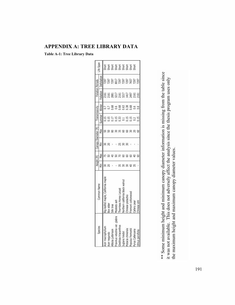
191
APPENDIX A: TREE LIBRARY DATA
Table A-1: Tree Library Data
Min
Max
Min
Max
Sum
mer
Win
ter
Folia
tion
Def
olia
tion
Ace
r m
acro
phyl
lum
Big
-lea
fed
map
le,
Cal
iforn
ia m
aple
3075
3050
0.15
0.7
2161
7297
Sho
rt
Ace
r ne
gund
oBox
eld
er20
5020
500.
150.
721
6172
97Sho
rt
Alb
izia
jul
ibriss
inSilk
tre
e-
40-
800.
170.
6828
8172
97Sho
rt
Frax
inus
vel
utin
a va
r. g
labr
aM
odes
to a
sh-
50-
300.
150.
632
1780
17Sho
rt
Gle
dits
ia t
riac
anth
osTh
ornl
ess
Hon
ey L
ocus
t35
7025
350.
330.
6821
6172
97Sho
rt
Jugl
ans
hind
sii
Nor
ther
n ca
lifor
nia
blac
k w
alnu
t30
6030
600.
10.
6332
1772
97Sho
rt
Pist
acia
chi
nens
isChi
nese
pis
tach
io30
6030
600.
150.
3814
1772
97Sho
rt
Popu
lus
frem
ontii
Frem
ont
cott
onw
ood
4060
-30
0.15
0.68
2497
7657
Sho
rt
Pyru
s Cal
lery
ana
Cal
lery
pea
r35
40-
200.
20.
621
6172
97Sho
rt
Ulm
us p
arvi
folia
Chi
nese
elm
-60
-60
0.15
0.6
2161
7297
Spe
cies
Com
mon
Nam
eLi
fe S
pan
Hei
ght
(ft)
Can
opy
Dia
met
er (
ft)
Tran
smis
sivi
tyFo
liatio
n Pe
riod
s
**
So
me
min
imu
m h
eig
ht
and
min
imu
m c
ano
py
dia
met
er i
nfo
rmat
ion i
s m
issi
ng f
rom
the
table
sin
ce
it w
as n
ot
avai
lable
. T
his
does
not
adver
sely
aff
ect
the
anal
ysi
s si
nce
the
thes
is p
rogra
m u
ses
only
th
e m
axim
um
hei
ght
and m
axim
um
can
opy d
iam
eter
val
ues
.

192
APPENDIX B: PROGRAM CODE
MODULE
Imports System.Math Module Module1 'Declare variables to be used in Module' Public EastTreeArray(39, 2) As Double Public SouthTreeArray(39, 2) As Double Public WestTreeArray(39, 2) As Double Public EastTreeArrayPrime(39, 2) As Double Public SouthTreeArrayPrime(39, 2) As Double Public WestTreeArrayPrime(39, 2) As Double Public EastTreeArrayPrimePrime(39, 2) As Double Public SouthTreeArrayPrimePrime(39, 2) As Double Public WestTreeArrayPrimePrime(39, 2) As Double Public EastShadeArray(19) As Double Public SouthShadeArray(19) As Double Public WestShadeArray(19) As Double Public EastQUnshadedArray(8759) As Double Public EastQShadedArray(8759) As Double Public SouthQUnshadedArray(8759) As Double Public SouthQShadedArray(8759) As Double Public WestQUnshadedArray(8759) As Double Public WestQShadedArray(8759) As Double 'Declare variables to be defined by user in Form 1 - Introduction' Public Latitude As Double = 33.93 'Latitude of selected city' Public Longitude As Double = 118.4 'Longitude of selected city' Public Insolation As New ArrayList Public DryBulbTemp As New ArrayList Public DiffuseRad As New ArrayList Public City As DataTable Public AST(8759) As Double 'Apparent Solar Time array' Public Altitude As New ArrayList Public Azimuth As New ArrayList

193
Public ElectricityRate As Double Public EastSurfaceAzimuth As Double = -90 Public SouthSurfaceAzimuth As Double = 0 Public WestSurfaceAzimuth As Double = 90 Public strTitle As String = "Warning!" Public Form1HelpString As String 'Declare variables to be defined and calculated in Form 2 - Building Information' Public NSWall As Integer 'North/South wall dimension' Public EWWall As Integer 'East/West wall dimension' Public FlrHt As Integer 'Floor Height dimension' Public NYard As Integer 'North yard dimension' Public EYard As Integer 'East yard dimension' Public SYard As Integer 'South yard dimension' Public WYard As Integer 'West yard dimension' Public Tin As Integer 'Indoor Temperature’ Public Form2HelpString As String 'Declare variables to be defined and calculated in Form 3 - East Wall Fenestration' Public ESouthDist As Integer 'East window distance from South Wall' Public EGroundDist As Integer 'East window height from ground' Public EWinWidth As Integer 'East window width dimension' Public EWinHeight As Integer 'East window height dimension' Public EUFen As Double 'East window U-value based on user input' Public ESHGC As Double 'East window Solar Heat Gain Coefficient’ Public EastWinArray(3, 2) As Double Public EastWinArrayPrime(3, 2) As Double Public EastWinArrayPrimePrime(3, 2) As Double Public EastAngleOfIncidence As Double Public Form3HelpString As String 'Declare variables to be defined and calculated in Form 4 - South Wall Fenestration' Public SWestDist As Integer 'Window distance from West Wall' Public SGroundDist As Integer 'South window height from ground' Public SWinWidth As Integer 'South window width dimension' Public SWinHeight As Integer 'South window height dimension' Public SUFen As Double 'South window U-value based on user input' Public SSHGC As Double 'South window Solar Heat Gain Coefficient’ Public SouthWinArray(3, 2) As Double Public SouthWinArrayPrime(3, 2) As Double Public SouthWinArrayPrimePrime(3, 2) As Double Public SouthAngleOfIncidence As Double Public Form4HelpString As String

194
'Declare variables to be defined and calculated in Form 5 - West Wall Fenestration' Public WNorthDist As Integer 'West window distance from North Wall' Public WGroundDist As Integer 'West window height from ground' Public WWinWidth As Integer 'West window width dimension' Public WWinHeight As Integer 'West window height dimension' Public WUFen As Double 'West window U-value based on user input' Public WSHGC As Double 'West window Solar Heat Gain Coefficient’ Public WestWinArray(3, 2) As Double Public WestWinArrayPrime(3, 2) As Double Public WestWinArrayPrimePrime(3, 2) As Double Public WestAngleOfIncidence As Double Public Form5HelpString As String 'Declare variables to be defined in Form 6 - Tree Selection' Public TreeData As DataTable Public TreeName As String Public TreeHeight As Integer 'Height of selected tree' Public TreeCanopyDiam As Integer 'Canopy diameter of selected tree' Public TreeRadius As Integer Public SummerTrans As Double 'Summer transmissivity of selected tree' Public WinterTrans As Double 'Winter transmissivity of selected tree' Public Transmissivity As Double 'Transmissivity will be assigned summer or winter based on hour' Public Foliation As Integer 'Foliation start date of selected tree' Public Defoliation As Integer 'Defoliation start date of selected tree' Public Description As String 'String that will hold information about tree to be displayed to user' Public Form6HelpString As String 'Declare variables to be used in Form 7 - Tree Placement' Public TreeX As Double 'Tree location x-coordinate' Public TreeY As Double 'Tree location y-coordinate' Public BranchHeight As Integer Public Form7HelpString As String Public Form8HelpString As String Public Sub EastScanline (ByVal WinWidth As Integer, ByVal WinHeight As Integer, ByVal
UFen As Double, ByVal SHGC As Double, ByVal TreeHeight As Integer, ByVal BranchHeight As Integer, ByVal TreeCanopyDiam As Integer, ByVal SummerTrans As Double, ByVal WinterTrans As Double, Foliation As Integer, ByVal Defoliation As Integer, ByVal hour As Integer, ByVal AngleOfIncidence As Double)
Dim Tin As Integer = 68 Dim i As Integer

195
Dim j As Integer Dim Area As Double 'Area of window' Dim TreeRadius As Integer Dim Slice As Integer = 19 Dim SliceHeight As Double Dim TotalShade As Double Dim TransDiff As Double TreeRadius = TreeCanopyDiam / 2 'Calculate total area of window' Area = WinWidth * WinHeight Dim QUnshaded As Double 'Instantaneous Energy Flow of unshaded window' Dim QShaded As Double 'Instantaneous Energy Flow of shaded window' Dim ShadeStart As Double 'Start coordinate of shade on window' Dim ShadeEnd As Double 'End coordinate of shade on window' TransDiff = (WinterTrans - SummerTrans) / 30 If hour < Foliation - 360 Then Transmissivity = WinterTrans ElseIf hour >= Foliation - 360 AndAlso hour <= Foliation + 360 Then If hour >= Foliation - 360 AndAlso hour < Foliation - 336 Then Transmissivity = WinterTrans - (TransDiff * 1) ElseIf hour >= Foliation - 336 AndAlso hour < Foliation - 312 Then Transmissivity = WinterTrans - (TransDiff * 2) ElseIf hour >= Foliation - 312 AndAlso hour < Foliation - 288 Then Transmissivity = WinterTrans - (TransDiff * 3) ElseIf hour >= Foliation - 288 AndAlso hour < Foliation - 264 Then Transmissivity = WinterTrans - (TransDiff * 4) ElseIf hour >= Foliation - 264 AndAlso hour < Foliation - 240 Then Transmissivity = WinterTrans - (TransDiff * 5) ElseIf hour >= Foliation - 240 AndAlso hour < Foliation - 216 Then Transmissivity = WinterTrans - (TransDiff * 6) ElseIf hour >= Foliation - 216 AndAlso hour < Foliation - 192 Then Transmissivity = WinterTrans - (TransDiff * 7) ElseIf hour >= Foliation - 192 AndAlso hour < Foliation - 168 Then Transmissivity = WinterTrans - (TransDiff * 8) ElseIf hour >= Foliation - 168 AndAlso hour < Foliation - 144 Then Transmissivity = WinterTrans - (TransDiff * 9) ElseIf hour >= Foliation - 144 AndAlso hour < Foliation - 120 Then Transmissivity = WinterTrans - (TransDiff * 10)
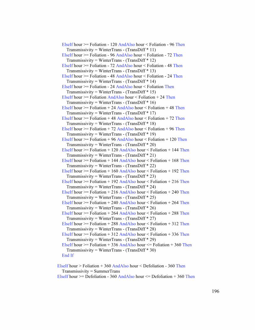
196
ElseIf hour >= Foliation - 120 AndAlso hour < Foliation - 96 Then Transmissivity = WinterTrans - (TransDiff * 11) ElseIf hour >= Foliation - 96 AndAlso hour < Foliation - 72 Then Transmissivity = WinterTrans - (TransDiff * 12) ElseIf hour >= Foliation - 72 AndAlso hour < Foliation - 48 Then Transmissivity = WinterTrans - (TransDiff * 13) ElseIf hour >= Foliation - 48 AndAlso hour < Foliation - 24 Then Transmissivity = WinterTrans - (TransDiff * 14) ElseIf hour >= Foliation - 24 AndAlso hour < Foliation Then Transmissivity = WinterTrans - (TransDiff * 15) ElseIf hour >= Foliation AndAlso hour < Foliation + 24 Then Transmissivity = WinterTrans - (TransDiff * 16) ElseIf hour >= Foliation + 24 AndAlso hour < Foliation + 48 Then Transmissivity = WinterTrans - (TransDiff * 17) ElseIf hour >= Foliation + 48 AndAlso hour < Foliation + 72 Then Transmissivity = WinterTrans - (TransDiff * 18) ElseIf hour >= Foliation + 72 AndAlso hour < Foliation + 96 Then Transmissivity = WinterTrans - (TransDiff * 19) ElseIf hour >= Foliation + 96 AndAlso hour < Foliation + 120 Then Transmissivity = WinterTrans - (TransDiff * 20) ElseIf hour >= Foliation + 120 AndAlso hour < Foliation + 144 Then Transmissivity = WinterTrans - (TransDiff * 21) ElseIf hour >= Foliation + 144 AndAlso hour < Foliation + 168 Then Transmissivity = WinterTrans - (TransDiff * 22) ElseIf hour >= Foliation + 160 AndAlso hour < Foliation + 192 Then Transmissivity = WinterTrans - (TransDiff * 23) ElseIf hour >= Foliation + 192 AndAlso hour < Foliation + 216 Then Transmissivity = WinterTrans - (TransDiff * 24) ElseIf hour >= Foliation + 216 AndAlso hour < Foliation + 240 Then Transmissivity = WinterTrans - (TransDiff * 25) ElseIf hour >= Foliation + 240 AndAlso hour < Foliation + 264 Then Transmissivity = WinterTrans - (TransDiff * 26) ElseIf hour >= Foliation + 264 AndAlso hour < Foliation + 288 Then Transmissivity = WinterTrans - (TransDiff * 27) ElseIf hour >= Foliation + 288 AndAlso hour < Foliation + 312 Then Transmissivity = WinterTrans - (TransDiff * 28) ElseIf hour >= Foliation + 312 AndAlso hour < Foliation + 336 Then Transmissivity = WinterTrans - (TransDiff * 29) ElseIf hour >= Foliation + 336 AndAlso hour <= Foliation + 360 Then Transmissivity = WinterTrans - (TransDiff * 30) End If ElseIf hour > Foliation + 360 AndAlso hour < Defoliation - 360 Then Transmissivity = SummerTrans ElseIf hour >= Defoliation - 360 AndAlso hour <= Defoliation + 360 Then
197
If hour >= Defoliation - 360 AndAlso hour < Defoliation - 336 Then Transmissivity = WinterTrans - (TransDiff * 30) ElseIf hour >= Defoliation - 336 AndAlso hour < Defoliation - 312 Then Transmissivity = WinterTrans - (TransDiff * 29) ElseIf hour >= Defoliation - 312 AndAlso hour < Defoliation - 288 Then Transmissivity = WinterTrans - (TransDiff * 28) ElseIf hour >= Defoliation - 288 AndAlso hour < Defoliation - 264 Then Transmissivity = WinterTrans - (TransDiff * 27) ElseIf hour >= Defoliation - 264 AndAlso hour < Defoliation - 240 Then Transmissivity = WinterTrans - (TransDiff * 26) ElseIf hour >= Defoliation - 240 AndAlso hour < Defoliation - 216 Then Transmissivity = WinterTrans - (TransDiff * 25) ElseIf hour >= Defoliation - 216 AndAlso hour < Defoliation - 192 Then Transmissivity = WinterTrans - (TransDiff * 24) ElseIf hour >= Defoliation - 192 AndAlso hour < Defoliation - 168 Then Transmissivity = WinterTrans - (TransDiff * 23) ElseIf hour >= Defoliation - 168 AndAlso hour < Defoliation - 144 Then Transmissivity = WinterTrans - (TransDiff * 22) ElseIf hour >= Defoliation - 144 AndAlso hour < Defoliation - 120 Then Transmissivity = WinterTrans - (TransDiff * 21) ElseIf hour >= Defoliation - 120 AndAlso hour < Defoliation - 96 Then Transmissivity = WinterTrans - (TransDiff * 20) ElseIf hour >= Defoliation - 96 AndAlso hour < Defoliation - 72 Then Transmissivity = WinterTrans - (TransDiff * 19) ElseIf hour >= Defoliation - 72 AndAlso hour < Defoliation - 48 Then Transmissivity = WinterTrans - (TransDiff * 18) ElseIf hour >= Defoliation - 48 AndAlso hour < Defoliation - 24 Then Transmissivity = WinterTrans - (TransDiff * 17) ElseIf hour >= Defoliation - 24 AndAlso hour < Defoliation Then Transmissivity = WinterTrans - (TransDiff * 16) ElseIf hour >= Defoliation AndAlso hour < Defoliation + 24 Then Transmissivity = WinterTrans - (TransDiff * 15) ElseIf hour >= Defoliation + 24 AndAlso hour < Defoliation + 48 Then Transmissivity = WinterTrans - (TransDiff * 14) ElseIf hour >= Defoliation + 48 AndAlso hour < Defoliation + 72 Then Transmissivity = WinterTrans - (TransDiff * 13) ElseIf hour >= Defoliation + 72 AndAlso hour < Defoliation + 96 Then Transmissivity = WinterTrans - (TransDiff * 12) ElseIf hour >= Defoliation + 96 AndAlso hour < Defoliation + 120 Then Transmissivity = WinterTrans - (TransDiff * 11) ElseIf hour >= Defoliation + 120 AndAlso hour < Defoliation + 144 Then Transmissivity = WinterTrans - (TransDiff * 10) ElseIf hour >= Defoliation + 144 AndAlso hour < Defoliation + 168 Then Transmissivity = WinterTrans - (TransDiff * 9) ElseIf hour >= Defoliation + 160 AndAlso hour < Defoliation + 192 Then Transmissivity = WinterTrans - (TransDiff * 8)

198
ElseIf hour >= Defoliation + 192 AndAlso hour < Defoliation + 216 Then Transmissivity = WinterTrans - (TransDiff * 7) ElseIf hour >= Defoliation + 216 AndAlso hour < Defoliation + 240 Then Transmissivity = WinterTrans - (TransDiff * 6) ElseIf hour >= Defoliation + 240 AndAlso hour < Defoliation + 264 Then Transmissivity = WinterTrans - (TransDiff * 5) ElseIf hour >= Defoliation + 264 AndAlso hour < Defoliation + 288 Then Transmissivity = WinterTrans - (TransDiff * 4) ElseIf hour >= Defoliation + 288 AndAlso hour < Defoliation + 312 Then Transmissivity = WinterTrans - (TransDiff * 3) ElseIf hour >= Defoliation + 312 AndAlso hour < Defoliation + 336 Then Transmissivity = WinterTrans - (TransDiff * 2) ElseIf hour >= Defoliation + 336 AndAlso hour < Defoliation + 360 Then Transmissivity = WinterTrans - (TransDiff * 1) End If ElseIf hour > Defoliation + 360 Then Transmissivity = WinterTrans End If 'Calculate instantaneous energy flow through unshaded window' QUnshaded = UFen * Area * (DryBulbTemp(hour) - Tin) + SHGC * Area *
(Insolation(hour) * Cos(EastAngleOfIncidence)) + SHGC * Area * (DiffuseRad(hour))
'Add instantaneous energy flow to the unshaded annual array' EastQUnshadedArray(hour) = QUnshaded 'Find shaded area of window from tree shadow' If EastTreeArrayPrimePrime(0, 1) < EastWinArrayPrimePrime(0, 1) Then For i = 2 To 21 If EastTreeArrayPrime(i, 2) > EastWinArrayPrime(1, 2) Then Exit For 'Check to see if z-coordinate of shadow is within window area' If EastTreeArrayPrime(i, 2) >= EastWinArrayPrime(0, 2) Then 'Check to see if shadow starts before scanline starting edge of window' 'If shadow starts before starting edge, assign scanline slice shadow start as
window edge' If EastTreeArrayPrime(i, 0) <= EastWinArrayPrime(0, 0) Then ShadeStart = EastWinArrayPrime(0, 0) 'Determine end location of shade segement'
199
If EastTreeArrayPrime(40 - i, 0) <= EastWinArrayPrime(3, 0) Then ShadeEnd = EastTreeArrayPrime(40 - i, 0) ElseIf EastTreeArrayPrime(40 - i, 0) >= EastWinArrayPrime(3, 0) Then ShadeEnd = EastWinArrayPrime(3, 0) End If ElseIf EastTreeArrayPrime(i, 0) <= EastWinArrayPrime(3, 0) Then 'Scan across window slice to see if/where the shadow starts on this slice' ShadeStart = EastTreeArrayPrime(i, 0) 'Determine end location of shade segement' If EastTreeArrayPrime(40 - i, 0) <= EastWinArrayPrime(3, 0) Then ShadeEnd = EastTreeArrayPrime(40 - i, 0) ElseIf EastTreeArrayPrime(40 - i, 0) >= EastWinArrayPrime(3, 0) Then ShadeEnd = EastWinArrayPrime(3, 0) End If End If End If If EastTreeArrayPrime(i + 1, 2) < EastWinArrayPrime(1, 2) Then SliceHeight = EastTreeArrayPrime(i + 1, 2) - EastTreeArrayPrime(i, 2) Else SliceHeight = EastWinArrayPrime(1, 2) - EastTreeArrayPrime(i, 2) End If EastShadeArray(i - 2) = (ShadeEnd - ShadeStart) * SliceHeight Next i Else For i = 2 To 21 If SouthTreeArrayPrime(i, 2) > EastWinArrayPrime(1, 2) Then Exit For 'Check to see if z-coordinate of shadow is within window area' If SouthTreeArrayPrime(i, 2) >= EastWinArrayPrime(0, 2) Then 'Check to see if shadow starts before scanline starting edge of window' 'If shadow starts before starting edge, assign scanline slice shadow start as
window edge' If SouthTreeArrayPrime(i, 0) <= EastWinArrayPrime(0, 0) Then ShadeStart = EastWinArrayPrime(0, 0)

200
'Determine end location of shade segement' If SouthTreeArrayPrime(40 - i, 0) <= EastWinArrayPrime(3, 0) Then ShadeEnd = SouthTreeArrayPrime(40 - i, 0) ElseIf SouthTreeArrayPrime(40 - i, 0) >= EastWinArrayPrime(3, 0) Then ShadeEnd = EastWinArrayPrime(3, 0) End If ElseIf SouthTreeArrayPrime(i, 0) <= EastWinArrayPrime(3, 0) Then 'Scan across window slice to see if/where the shadow starts on this slice' ShadeStart = SouthTreeArrayPrime(i, 0) 'Determine end location of shade segement' If SouthTreeArrayPrime(40 - i, 0) <= EastWinArrayPrime(3, 0) Then ShadeEnd = SouthTreeArrayPrime(40 - i, 0) ElseIf SouthTreeArrayPrime(40 - i, 0) >= EastWinArrayPrime(3, 0) Then ShadeEnd = EastWinArrayPrime(3, 0) End If End If End If If SouthTreeArrayPrime(i + 1, 2) < EastWinArrayPrime(1, 2) Then SliceHeight = SouthTreeArrayPrime(i + 1, 2) - SouthTreeArrayPrime(i, 2) Else SliceHeight = SouthWinArrayPrime(1, 2) - EastTreeArrayPrime(i, 2) End If EastShadeArray(i - 2) = (ShadeEnd - ShadeStart) * SliceHeight Next i End If 'Calculate total shaded area of window from tree polygon' For j = 0 To Slice TotalShade += EastShadeArray(j) Next j If TotalShade > 0 Then 'Calculate instantaneous energy flow through shaded window' QShaded = UFen * Area * (DryBulbTemp(hour) - Tin) + SHGC * TotalShade *
Transmissivity * ((Insolation(hour) * Cos(AngleOfIncidence)) + DiffuseRad(hour)) + SHGC * (Area - TotalShade) * Transmissivity * ((Insolation(hour) * Cos(AngleOfIncidence)) + DiffuseRad(hour))
Else

201
QShaded = QUnshaded End If 'Add instantaneous energy flow to the shaded annual array' EastQShadedArray(hour) = QShaded End Sub Public Sub SouthScanline (ByVal WinWidth As Integer, ByVal WinHeight As Integer,
ByVal UFen As Double, ByVal SHGC As Double, ByVal TreeHeight As Integer, ByVal BranchHeight As Integer, ByVal TreeCanopyDiam As Integer, ByVal SummerTrans As Double, ByVal WinterTrans As Double, ByVal Foliation As Integer, ByVal Defoliation As Integer, ByVal hour As Integer, ByVal AngleOfIncidence As Double)
Dim Tin As Integer = 68 Dim i As Integer Dim j As Integer Dim Area As Double 'Area of window' Dim Slice As Integer = 19 Dim SliceHeight As Double Dim TotalShade As Double Dim TransDiff As Double 'Calculate total area of window' Area = WinWidth * WinHeight Dim QUnshaded As Double 'Instantaneous Energy Flow of unshaded window' Dim QShaded As Double 'Instantaneous Energy Flow of shaded window' Dim ShadeStart As Double 'Start coordinate of shade on window' Dim ShadeEnd As Double 'End coordinate of shade on window' TransDiff = (WinterTrans - SummerTrans) / 30 'Assign Transmissivity value based on time of year' If hour < Foliation - 360 Then Transmissivity = WinterTrans ElseIf hour >= Foliation - 360 AndAlso hour <= Foliation + 360 Then If hour >= Foliation - 360 AndAlso hour < Foliation - 336 Then Transmissivity = WinterTrans - (TransDiff * 1)
202
ElseIf hour >= Foliation - 336 AndAlso hour < Foliation - 312 Then Transmissivity = WinterTrans - (TransDiff * 2) ElseIf hour >= Foliation - 312 AndAlso hour < Foliation - 288 Then Transmissivity = WinterTrans - (TransDiff * 3) ElseIf hour >= Foliation - 288 AndAlso hour < Foliation - 264 Then Transmissivity = WinterTrans - (TransDiff * 4) ElseIf hour >= Foliation - 264 AndAlso hour < Foliation - 240 Then Transmissivity = WinterTrans - (TransDiff * 5) ElseIf hour >= Foliation - 240 AndAlso hour < Foliation - 216 Then Transmissivity = WinterTrans - (TransDiff * 6) ElseIf hour >= Foliation - 216 AndAlso hour < Foliation - 192 Then Transmissivity = WinterTrans - (TransDiff * 7) ElseIf hour >= Foliation - 192 AndAlso hour < Foliation - 168 Then Transmissivity = WinterTrans - (TransDiff * 8) ElseIf hour >= Foliation - 168 AndAlso hour < Foliation - 144 Then Transmissivity = WinterTrans - (TransDiff * 9) ElseIf hour >= Foliation - 144 AndAlso hour < Foliation - 120 Then Transmissivity = WinterTrans - (TransDiff * 10) ElseIf hour >= Foliation - 120 AndAlso hour < Foliation - 96 Then Transmissivity = WinterTrans - (TransDiff * 11) ElseIf hour >= Foliation - 96 AndAlso hour < Foliation - 72 Then Transmissivity = WinterTrans - (TransDiff * 12) ElseIf hour >= Foliation - 72 AndAlso hour < Foliation - 48 Then Transmissivity = WinterTrans - (TransDiff * 13) ElseIf hour >= Foliation - 48 AndAlso hour < Foliation - 24 Then Transmissivity = WinterTrans - (TransDiff * 14) ElseIf hour >= Foliation - 24 AndAlso hour < Foliation Then Transmissivity = WinterTrans - (TransDiff * 15) ElseIf hour >= Foliation AndAlso hour < Foliation + 24 Then Transmissivity = WinterTrans - (TransDiff * 16) ElseIf hour >= Foliation + 24 AndAlso hour < Foliation + 48 Then Transmissivity = WinterTrans - (TransDiff * 17) ElseIf hour >= Foliation + 48 AndAlso hour < Foliation + 72 Then Transmissivity = WinterTrans - (TransDiff * 18) ElseIf hour >= Foliation + 72 AndAlso hour < Foliation + 96 Then Transmissivity = WinterTrans - (TransDiff * 19) ElseIf hour >= Foliation + 96 AndAlso hour < Foliation + 120 Then Transmissivity = WinterTrans - (TransDiff * 20) ElseIf hour >= Foliation + 120 AndAlso hour < Foliation + 144 Then Transmissivity = WinterTrans - (TransDiff * 21) ElseIf hour >= Foliation + 144 AndAlso hour < Foliation + 168 Then Transmissivity = WinterTrans - (TransDiff * 22) ElseIf hour >= Foliation + 160 AndAlso hour < Foliation + 192 Then Transmissivity = WinterTrans - (TransDiff * 23) ElseIf hour >= Foliation + 192 AndAlso hour < Foliation + 216 Then Transmissivity = WinterTrans - (TransDiff * 24)
203
ElseIf hour >= Foliation + 216 AndAlso hour < Foliation + 240 Then Transmissivity = WinterTrans - (TransDiff * 25) ElseIf hour >= Foliation + 240 AndAlso hour < Foliation + 264 Then Transmissivity = WinterTrans - (TransDiff * 26) ElseIf hour >= Foliation + 264 AndAlso hour < Foliation + 288 Then Transmissivity = WinterTrans - (TransDiff * 27) ElseIf hour >= Foliation + 288 AndAlso hour < Foliation + 312 Then Transmissivity = WinterTrans - (TransDiff * 28) ElseIf hour >= Foliation + 312 AndAlso hour < Foliation + 336 Then Transmissivity = WinterTrans - (TransDiff * 29) ElseIf hour >= Foliation + 336 AndAlso hour <= Foliation + 360 Then Transmissivity = WinterTrans - (TransDiff * 30) End If ElseIf hour > Foliation + 360 AndAlso hour < Defoliation - 360 Then Transmissivity = SummerTrans ElseIf hour >= Defoliation - 360 AndAlso hour <= Defoliation + 360 Then If hour >= Defoliation - 360 AndAlso hour < Defoliation - 336 Then Transmissivity = WinterTrans - (TransDiff * 30) ElseIf hour >= Defoliation - 336 AndAlso hour < Defoliation - 312 Then Transmissivity = WinterTrans - (TransDiff * 29) ElseIf hour >= Defoliation - 312 AndAlso hour < Defoliation - 288 Then Transmissivity = WinterTrans - (TransDiff * 28) ElseIf hour >= Defoliation - 288 AndAlso hour < Defoliation - 264 Then Transmissivity = WinterTrans - (TransDiff * 27) ElseIf hour >= Defoliation - 264 AndAlso hour < Defoliation - 240 Then Transmissivity = WinterTrans - (TransDiff * 26) ElseIf hour >= Defoliation - 240 AndAlso hour < Defoliation - 216 Then Transmissivity = WinterTrans - (TransDiff * 25) ElseIf hour >= Defoliation - 216 AndAlso hour < Defoliation - 192 Then Transmissivity = WinterTrans - (TransDiff * 24) ElseIf hour >= Defoliation - 192 AndAlso hour < Defoliation - 168 Then Transmissivity = WinterTrans - (TransDiff * 23) ElseIf hour >= Defoliation - 168 AndAlso hour < Defoliation - 144 Then Transmissivity = WinterTrans - (TransDiff * 22) ElseIf hour >= Defoliation - 144 AndAlso hour < Defoliation - 120 Then Transmissivity = WinterTrans - (TransDiff * 21) ElseIf hour >= Defoliation - 120 AndAlso hour < Defoliation - 96 Then Transmissivity = WinterTrans - (TransDiff * 20) ElseIf hour >= Defoliation - 96 AndAlso hour < Defoliation - 72 Then Transmissivity = WinterTrans - (TransDiff * 19) ElseIf hour >= Defoliation - 72 AndAlso hour < Defoliation - 48 Then Transmissivity = WinterTrans - (TransDiff * 18) ElseIf hour >= Defoliation - 48 AndAlso hour < Defoliation - 24 Then Transmissivity = WinterTrans - (TransDiff * 17)
204
ElseIf hour >= Defoliation - 24 AndAlso hour < Defoliation Then Transmissivity = WinterTrans - (TransDiff * 16) ElseIf hour >= Defoliation AndAlso hour < Defoliation + 24 Then Transmissivity = WinterTrans - (TransDiff * 15) ElseIf hour >= Defoliation + 24 AndAlso hour < Defoliation + 48 Then Transmissivity = WinterTrans - (TransDiff * 14) ElseIf hour >= Defoliation + 48 AndAlso hour < Defoliation + 72 Then Transmissivity = WinterTrans - (TransDiff * 13) ElseIf hour >= Defoliation + 72 AndAlso hour < Defoliation + 96 Then Transmissivity = WinterTrans - (TransDiff * 12) ElseIf hour >= Defoliation + 96 AndAlso hour < Defoliation + 120 Then Transmissivity = WinterTrans - (TransDiff * 11) ElseIf hour >= Defoliation + 120 AndAlso hour < Defoliation + 144 Then Transmissivity = WinterTrans - (TransDiff * 10) ElseIf hour >= Defoliation + 144 AndAlso hour < Defoliation + 168 Then Transmissivity = WinterTrans - (TransDiff * 9) ElseIf hour >= Defoliation + 160 AndAlso hour < Defoliation + 192 Then Transmissivity = WinterTrans - (TransDiff * 8) ElseIf hour >= Defoliation + 192 AndAlso hour < Defoliation + 216 Then Transmissivity = WinterTrans - (TransDiff * 7) ElseIf hour >= Defoliation + 216 AndAlso hour < Defoliation + 240 Then Transmissivity = WinterTrans - (TransDiff * 6) ElseIf hour >= Defoliation + 240 AndAlso hour < Defoliation + 264 Then Transmissivity = WinterTrans - (TransDiff * 5) ElseIf hour >= Defoliation + 264 AndAlso hour < Defoliation + 288 Then Transmissivity = WinterTrans - (TransDiff * 4) ElseIf hour >= Defoliation + 288 AndAlso hour < Defoliation + 312 Then Transmissivity = WinterTrans - (TransDiff * 3) ElseIf hour >= Defoliation + 312 AndAlso hour < Defoliation + 336 Then Transmissivity = WinterTrans - (TransDiff * 2) ElseIf hour >= Defoliation + 336 AndAlso hour < Defoliation + 360 Then Transmissivity = WinterTrans - (TransDiff * 1) End If ElseIf hour > Defoliation + 360 Then Transmissivity = WinterTrans End If 'Calculate instantaneous energy flow through unshaded window' QUnshaded = UFen * Area * (DryBulbTemp(hour) - Tin) + SHGC * Area *
(Insolation(hour) * Cos(AngleOfIncidence)) + SHGC * Area * DiffuseRad(hour)
'Add instantaneous energy flow to the unshaded annual array' SouthQUnshadedArray(hour) = QUnshaded

205
'Find shaded area of window from tree shadow' If SouthTreeArrayPrimePrime(0, 1) < SouthWinArrayPrimePrime(0, 1) Then For i = 2 To 21 If SouthTreeArrayPrime(i, 2) > SouthWinArrayPrime(1, 2) Then Exit For 'Check to see if z-coordinate of shadow is within window area' If SouthTreeArrayPrime(i, 2) >= SouthWinArrayPrime(0, 2) Then 'Check to see if shadow starts before scanline starting edge of window' 'If shadow starts before starting edge, assign scanline slice shadow start as
window edge' If SouthTreeArrayPrime(i, 0) <= SouthWinArrayPrime(0, 0) Then ShadeStart = SouthWinArrayPrime(0, 0) 'Determine end location of shade segement' If SouthTreeArrayPrime(40 - i, 0) <= SouthWinArrayPrime(3, 0) Then ShadeEnd = SouthTreeArrayPrime(40 - i, 0) ElseIf SouthTreeArrayPrime(40 - i, 0) > SouthWinArrayPrime(3, 0) Then ShadeEnd = SouthWinArrayPrime(3, 0) End If ElseIf SouthTreeArrayPrime(i, 0) <= SouthWinArrayPrime(3, 0) Then 'Scan across window slice to see if/where the shadow starts on this slice' ShadeStart = SouthTreeArrayPrime(i, 0) 'Determine end location of shade segement' If SouthTreeArrayPrime(40 - i, 0) <= SouthWinArrayPrime(3, 0) Then ShadeEnd = SouthTreeArrayPrime(40 - i, 0) ElseIf SouthTreeArrayPrime(40 - i, 0) > SouthWinArrayPrime(3, 0) Then ShadeEnd = SouthWinArrayPrime(3, 0) End If End If End If If SouthTreeArrayPrime(i + 1, 2) < SouthWinArrayPrime(1, 2) Then SliceHeight = SouthTreeArrayPrime(i + 1, 2) - SouthTreeArrayPrime(i, 2) Else SliceHeight = SouthWinArrayPrime(1, 2) - SouthTreeArrayPrime(i, 2) End If SouthShadeArray(i - 2) = (ShadeEnd - ShadeStart) * SliceHeight

206
Next i Else End If 'Calculate total shaded area of window from tree polygon' For j = 0 To Slice TotalShade += SouthShadeArray(j) Next j If TotalShade > 0 Then 'Calculate instantaneous energy flow through shaded window'
QShaded = UFen * Area * (DryBulbTemp(hour) - Tin) + SHGC * TotalShade * Transmissivity * ((Insolation(hour) * Cos(AngleOfIncidence)) + DiffuseRad(hour)) + SHGC * (Area - TotalShade) * Transmissivity * ((Insolation(hour) * Cos(AngleOfIncidence)) + DiffuseRad(hour))
Else QShaded = QUnshaded End If 'Add instantaneous energy flow to the shaded annual array' SouthQShadedArray(hour) = QShaded End Sub Public Sub WestScanline(ByVal WinWidth As Integer, ByVal WinHeight As Integer,
ByVal UFen As Double, ByVal SHGC As Double, ByVal TreeHeight As Integer, ByVal BranchHeight As Integer, ByVal TreeCanopyDiam As Integer, ByVal SummerTrans As Double, ByVal WinterTrans As Double, ByVal Foliation As Integer, ByVal Defoliation As Integer, ByVal hour As Integer, ByVal AngleOfIncidence As Double)
Dim Tin As Integer = 68 Dim i As Integer Dim j As Integer Dim Area As Double 'Area of window' Dim TreeRadius As Integer Dim Slice As Integer = 19 Dim SliceHeight As Double Dim TotalShade As Double
207
Dim TransDiff As Double TreeRadius = TreeCanopyDiam / 2 'Calculate total area of window' Area = WinWidth * WinHeight Dim QUnshaded As Double 'Instantaneous Energy Flow of unshaded window' Dim QShaded As Double 'Instantaneous Energy Flow of shaded window' Dim ShadeStart As Double 'Start coordinate of shade on window' Dim ShadeEnd As Double 'End coordinate of shade on window' TransDiff = (WinterTrans - SummerTrans) / 30 If hour < Foliation - 360 Then Transmissivity = WinterTrans ElseIf hour >= Foliation - 360 AndAlso hour <= Foliation + 360 Then If hour >= Foliation - 360 AndAlso hour < Foliation - 336 Then Transmissivity = WinterTrans - (TransDiff * 1) ElseIf hour >= Foliation - 336 AndAlso hour < Foliation - 312 Then Transmissivity = WinterTrans - (TransDiff * 2) ElseIf hour >= Foliation - 312 AndAlso hour < Foliation - 288 Then Transmissivity = WinterTrans - (TransDiff * 3) ElseIf hour >= Foliation - 288 AndAlso hour < Foliation - 264 Then Transmissivity = WinterTrans - (TransDiff * 4) ElseIf hour >= Foliation - 264 AndAlso hour < Foliation - 240 Then Transmissivity = WinterTrans - (TransDiff * 5) ElseIf hour >= Foliation - 240 AndAlso hour < Foliation - 216 Then Transmissivity = WinterTrans - (TransDiff * 6) ElseIf hour >= Foliation - 216 AndAlso hour < Foliation - 192 Then Transmissivity = WinterTrans - (TransDiff * 7) ElseIf hour >= Foliation - 192 AndAlso hour < Foliation - 168 Then Transmissivity = WinterTrans - (TransDiff * 8) ElseIf hour >= Foliation - 168 AndAlso hour < Foliation - 144 Then Transmissivity = WinterTrans - (TransDiff * 9) ElseIf hour >= Foliation - 144 AndAlso hour < Foliation - 120 Then Transmissivity = WinterTrans - (TransDiff * 10) ElseIf hour >= Foliation - 120 AndAlso hour < Foliation - 96 Then Transmissivity = WinterTrans - (TransDiff * 11) ElseIf hour >= Foliation - 96 AndAlso hour < Foliation - 72 Then Transmissivity = WinterTrans - (TransDiff * 12) ElseIf hour >= Foliation - 72 AndAlso hour < Foliation - 48 Then Transmissivity = WinterTrans - (TransDiff * 13) ElseIf hour >= Foliation - 48 AndAlso hour < Foliation - 24 Then
208
Transmissivity = WinterTrans - (TransDiff * 14) ElseIf hour >= Foliation - 24 AndAlso hour < Foliation Then Transmissivity = WinterTrans - (TransDiff * 15) ElseIf hour >= Foliation AndAlso hour < Foliation + 24 Then Transmissivity = WinterTrans - (TransDiff * 16) ElseIf hour >= Foliation + 24 AndAlso hour < Foliation + 48 Then Transmissivity = WinterTrans - (TransDiff * 17) ElseIf hour >= Foliation + 48 AndAlso hour < Foliation + 72 Then Transmissivity = WinterTrans - (TransDiff * 18) ElseIf hour >= Foliation + 72 AndAlso hour < Foliation + 96 Then Transmissivity = WinterTrans - (TransDiff * 19) ElseIf hour >= Foliation + 96 AndAlso hour < Foliation + 120 Then Transmissivity = WinterTrans - (TransDiff * 20) ElseIf hour >= Foliation + 120 AndAlso hour < Foliation + 144 Then Transmissivity = WinterTrans - (TransDiff * 21) ElseIf hour >= Foliation + 144 AndAlso hour < Foliation + 168 Then Transmissivity = WinterTrans - (TransDiff * 22) ElseIf hour >= Foliation + 160 AndAlso hour < Foliation + 192 Then Transmissivity = WinterTrans - (TransDiff * 23) ElseIf hour >= Foliation + 192 AndAlso hour < Foliation + 216 Then Transmissivity = WinterTrans - (TransDiff * 24) ElseIf hour >= Foliation + 216 AndAlso hour < Foliation + 240 Then Transmissivity = WinterTrans - (TransDiff * 25) ElseIf hour >= Foliation + 240 AndAlso hour < Foliation + 264 Then Transmissivity = WinterTrans - (TransDiff * 26) ElseIf hour >= Foliation + 264 AndAlso hour < Foliation + 288 Then Transmissivity = WinterTrans - (TransDiff * 27) ElseIf hour >= Foliation + 288 AndAlso hour < Foliation + 312 Then Transmissivity = WinterTrans - (TransDiff * 28) ElseIf hour >= Foliation + 312 AndAlso hour < Foliation + 336 Then Transmissivity = WinterTrans - (TransDiff * 29) ElseIf hour >= Foliation + 336 AndAlso hour <= Foliation + 360 Then Transmissivity = WinterTrans - (TransDiff * 30) End If ElseIf hour > Foliation + 360 AndAlso hour < Defoliation - 360 Then Transmissivity = SummerTrans ElseIf hour >= Defoliation - 360 AndAlso hour <= Defoliation + 360 Then If hour >= Defoliation - 360 AndAlso hour < Defoliation - 336 Then Transmissivity = WinterTrans - (TransDiff * 30) ElseIf hour >= Defoliation - 336 AndAlso hour < Defoliation - 312 Then Transmissivity = WinterTrans - (TransDiff * 29) ElseIf hour >= Defoliation - 312 AndAlso hour < Defoliation - 288 Then Transmissivity = WinterTrans - (TransDiff * 28) ElseIf hour >= Defoliation - 288 AndAlso hour < Defoliation - 264 Then
209
Transmissivity = WinterTrans - (TransDiff * 27) ElseIf hour >= Defoliation - 264 AndAlso hour < Defoliation - 240 Then Transmissivity = WinterTrans - (TransDiff * 26) ElseIf hour >= Defoliation - 240 AndAlso hour < Defoliation - 216 Then Transmissivity = WinterTrans - (TransDiff * 25) ElseIf hour >= Defoliation - 216 AndAlso hour < Defoliation - 192 Then Transmissivity = WinterTrans - (TransDiff * 24) ElseIf hour >= Defoliation - 192 AndAlso hour < Defoliation - 168 Then Transmissivity = WinterTrans - (TransDiff * 23) ElseIf hour >= Defoliation - 168 AndAlso hour < Defoliation - 144 Then Transmissivity = WinterTrans - (TransDiff * 22) ElseIf hour >= Defoliation - 144 AndAlso hour < Defoliation - 120 Then Transmissivity = WinterTrans - (TransDiff * 21) ElseIf hour >= Defoliation - 120 AndAlso hour < Defoliation - 96 Then Transmissivity = WinterTrans - (TransDiff * 20) ElseIf hour >= Defoliation - 96 AndAlso hour < Defoliation - 72 Then Transmissivity = WinterTrans - (TransDiff * 19) ElseIf hour >= Defoliation - 72 AndAlso hour < Defoliation - 48 Then Transmissivity = WinterTrans - (TransDiff * 18) ElseIf hour >= Defoliation - 48 AndAlso hour < Defoliation - 24 Then Transmissivity = WinterTrans - (TransDiff * 17) ElseIf hour >= Defoliation - 24 AndAlso hour < Defoliation Then Transmissivity = WinterTrans - (TransDiff * 16) ElseIf hour >= Defoliation AndAlso hour < Defoliation + 24 Then Transmissivity = WinterTrans - (TransDiff * 15) ElseIf hour >= Defoliation + 24 AndAlso hour < Defoliation + 48 Then Transmissivity = WinterTrans - (TransDiff * 14) ElseIf hour >= Defoliation + 48 AndAlso hour < Defoliation + 72 Then Transmissivity = WinterTrans - (TransDiff * 13) ElseIf hour >= Defoliation + 72 AndAlso hour < Defoliation + 96 Then Transmissivity = WinterTrans - (TransDiff * 12) ElseIf hour >= Defoliation + 96 AndAlso hour < Defoliation + 120 Then Transmissivity = WinterTrans - (TransDiff * 11) ElseIf hour >= Defoliation + 120 AndAlso hour < Defoliation + 144 Then Transmissivity = WinterTrans - (TransDiff * 10) ElseIf hour >= Defoliation + 144 AndAlso hour < Defoliation + 168 Then Transmissivity = WinterTrans - (TransDiff * 9) ElseIf hour >= Defoliation + 160 AndAlso hour < Defoliation + 192 Then Transmissivity = WinterTrans - (TransDiff * 8) ElseIf hour >= Defoliation + 192 AndAlso hour < Defoliation + 216 Then Transmissivity = WinterTrans - (TransDiff * 7) ElseIf hour >= Defoliation + 216 AndAlso hour < Defoliation + 240 Then Transmissivity = WinterTrans - (TransDiff * 6) ElseIf hour >= Defoliation + 240 AndAlso hour < Defoliation + 264 Then Transmissivity = WinterTrans - (TransDiff * 5) ElseIf hour >= Defoliation + 264 AndAlso hour < Defoliation + 288 Then

210
Transmissivity = WinterTrans - (TransDiff * 4) ElseIf hour >= Defoliation + 288 AndAlso hour < Defoliation + 312 Then Transmissivity = WinterTrans - (TransDiff * 3) ElseIf hour >= Defoliation + 312 AndAlso hour < Defoliation + 336 Then Transmissivity = WinterTrans - (TransDiff * 2) ElseIf hour >= Defoliation + 336 AndAlso hour < Defoliation + 360 Then Transmissivity = WinterTrans - (TransDiff * 1) End If ElseIf hour > Defoliation + 360 Then Transmissivity = WinterTrans End If 'Calculate instantaneous energy flow through unshaded window' QUnshaded = UFen * Area * (DryBulbTemp(hour) - Tin) _ + SHGC * Area * (Insolation(hour) * Cos(AngleOfIncidence)) _ + SHGC * Area * DiffuseRad(hour) 'Add instantaneous energy flow to the unshaded annual array' WestQUnshadedArray(hour) = QUnshaded 'Find shaded area of window from tree shadow' If WestTreeArrayPrimePrime(0, 1) < WestWinArrayPrimePrime(0, 1) Then For i = 2 To 21 If WestTreeArrayPrime(i, 2) > WestWinArrayPrime(1, 2) Then Exit For 'Check to see if z-coordinate of shadow is within window area' If WestTreeArrayPrime(i, 2) >= WestWinArrayPrime(0, 2) Then 'Check to see if shadow starts before scanline starting edge of window' 'If shadow starts before starting edge, assign scanline slice shadow start as
window edge' If WestTreeArrayPrime(i, 0) <= WestWinArrayPrime(0, 0) Then ShadeStart = WestWinArrayPrime(0, 0) 'Determine end location of shade segment' If WestTreeArrayPrime(40 - i, 0) < WestWinArrayPrime(3, 0) Then ShadeEnd = WestTreeArrayPrime(40 - i, 0) ElseIf WestTreeArrayPrime(40 - i, 0) >= WestWinArrayPrime(3, 0) Then ShadeEnd = WestWinArrayPrime(3, 0) End If ElseIf WestTreeArrayPrime(i, 0) >= WestWinArrayPrime(3, 0) Then
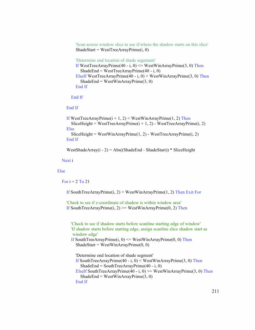
211
'Scan across window slice to see if/where the shadow starts on this slice' ShadeStart = WestTreeArrayPrime(i, 0) 'Determine end location of shade segement' If WestTreeArrayPrime(40 - i, 0) <= WestWinArrayPrime(3, 0) Then ShadeEnd = WestTreeArrayPrime(40 - i, 0) ElseIf WestTreeArrayPrime(40 - i, 0) > WestWinArrayPrime(3, 0) Then ShadeEnd = WestWinArrayPrime(3, 0) End If End If End If If WestTreeArrayPrime(i + 1, 2) < WestWinArrayPrime(1, 2) Then SliceHeight = WestTreeArrayPrime(i + 1, 2) - WestTreeArrayPrime(i, 2) Else SliceHeight = WestWinArrayPrime(1, 2) - WestTreeArrayPrime(i, 2) End If WestShadeArray(i - 2) = Abs((ShadeEnd - ShadeStart)) * SliceHeight Next i Else For i = 2 To 21 If SouthTreeArrayPrime(i, 2) > WestWinArrayPrime(1, 2) Then Exit For 'Check to see if z-coordinate of shadow is within window area' If SouthTreeArrayPrime(i, 2) >= WestWinArrayPrime(0, 2) Then 'Check to see if shadow starts before scanline starting edge of window' 'If shadow starts before starting edge, assign scanline slice shadow start as
window edge' If SouthTreeArrayPrime(i, 0) <= WestWinArrayPrime(0, 0) Then ShadeStart = WestWinArrayPrime(0, 0) 'Determine end location of shade segment' If SouthTreeArrayPrime(40 - i, 0) < WestWinArrayPrime(3, 0) Then ShadeEnd = SouthTreeArrayPrime(40 - i, 0) ElseIf SouthTreeArrayPrime(40 - i, 0) >= WestWinArrayPrime(3, 0) Then ShadeEnd = WestWinArrayPrime(3, 0) End If

212
ElseIf SouthTreeArrayPrime(i, 0) >= WestWinArrayPrime(3, 0) Then 'Scan across window slice to see if/where the shadow starts on this slice' ShadeStart = SouthTreeArrayPrime(i, 0) 'Determine end location of shade segement' If SouthTreeArrayPrime(40 - i, 0) <= WestWinArrayPrime(3, 0) Then ShadeEnd = SouthTreeArrayPrime(40 - i, 0) ElseIf SouthTreeArrayPrime(40 - i, 0) > WestWinArrayPrime(3, 0) Then ShadeEnd = WestWinArrayPrime(3, 0) End If End If End If If SouthTreeArrayPrime(i + 1, 2) < WestWinArrayPrime(1, 2) Then SliceHeight = SouthTreeArrayPrime(i + 1, 2) - SouthTreeArrayPrime(i, 2) Else SliceHeight = WestWinArrayPrime(1, 2) - SouthTreeArrayPrime(i, 2) End If WestShadeArray(i - 2) = Abs((ShadeEnd - ShadeStart)) * SliceHeight Next i End If 'Calculate total shaded area of window from tree polygon' For j = 0 To Slice TotalShade += WestShadeArray(j) Next j If TotalShade > 0 Then 'Calculate instantaneous energy flow through shaded window' QShaded = UFen * Area * (DryBulbTemp(hour) - Tin) + SHGC * TotalShade *
Transmissivity * ((Insolation(hour) * Cos(AngleOfIncidence)) + DiffuseRad(hour)) + SHGC * (Area - TotalShade) * Transmissivity * ((Insolation(hour) * Cos(AngleOfIncidence)) + DiffuseRad(hour))
Else QShaded = QUnshaded End If 'Add instantaneous energy flow to the shaded annual array' WestQShadedArray(hour) = QShaded End Sub End Module

213
FORM 1 – WELCOME SCREEN
Imports System.Math Public Class Form1 Private Sub TxtBxElecRate_TextChanged(ByVal sender As System.Object, ByVal e As
System.EventArgs) Handles TxtBxElecRate.TextChanged 'Assign electricity rate based on user input' ElectricityRate = Val(TxtBxElecRate.Text) End Sub Private Sub TxtBxElectRate_Validated(ByVal sender As Object, ByVal e As
System.EventArgs) Handles TxtBxElecRate.Validated Me.ErrorProvider1.SetError(TxtBxElecRate, "") End Sub Private Sub TxtBxElecRate_Validating(ByVal sender As Object, ByVal e As
System.ComponentModel.CancelEventArgs) Handles TxtBxElecRate.Validating
Try If Me.TxtBxElecRate.Text.Length = 0 Then Me.ErrorProvider1.SetError(Me.TxtBxElecRate, "Please Enter a value") Throw New Exception("Please enter a value") ElseIf Not IsNumeric(TxtBxElecRate.Text) Then Me.ErrorProvider1.SetError(Me.TxtBxElecRate, "Please Enter a Numeric
Value!") Throw New Exception("Please enter a numeric value") End If Catch ex As Exception MsgBox(ex.Message) End Try End Sub Private Sub Los_AngelesBindingNavigatorSaveItem_Click(ByVal sender As
System.Object, ByVal e As System.EventArgs) Me.Validate()
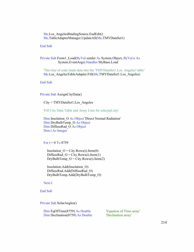
214
Me.Los_AngelesBindingSource.EndEdit() Me.TableAdapterManager.UpdateAll(Me.TMYDataSet1) End Sub Private Sub Form1_Load(ByVal sender As System.Object, ByVal e As
System.EventArgs) Handles MyBase.Load 'This line of code loads data into the 'TMYDataSet1.Los_Angeles' table’ Me.Los_AngelesTableAdapter.Fill(Me.TMYDataSet1.Los_Angeles) End Sub Private Sub AssignCityData() City = TMYDataSet1.Los_Angeles 'Fill City Data Table and Array Lists for selected city' Dim Insolation_O As Object 'Direct Normal Radiation' Dim DryBulbTemp_O As Object Dim DiffuseRad_O As Object Dim i As Integer For i = 0 To 8759 Insolation_O = City.Rows(i).Item(0) DiffuseRad_O = City.Rows(i).Item(1) DryBulbTemp_O = City.Rows(i).Item(2) Insolation.Add(Insolation_O) DiffuseRad.Add(DiffuseRad_O) DryBulbTemp.Add(DryBulbTemp_O) Next i End Sub Private Sub SolarAngles() Dim EqOfTime(8759) As Double 'Equation of Time array' Dim Declination(8759) As Double 'Declination array'
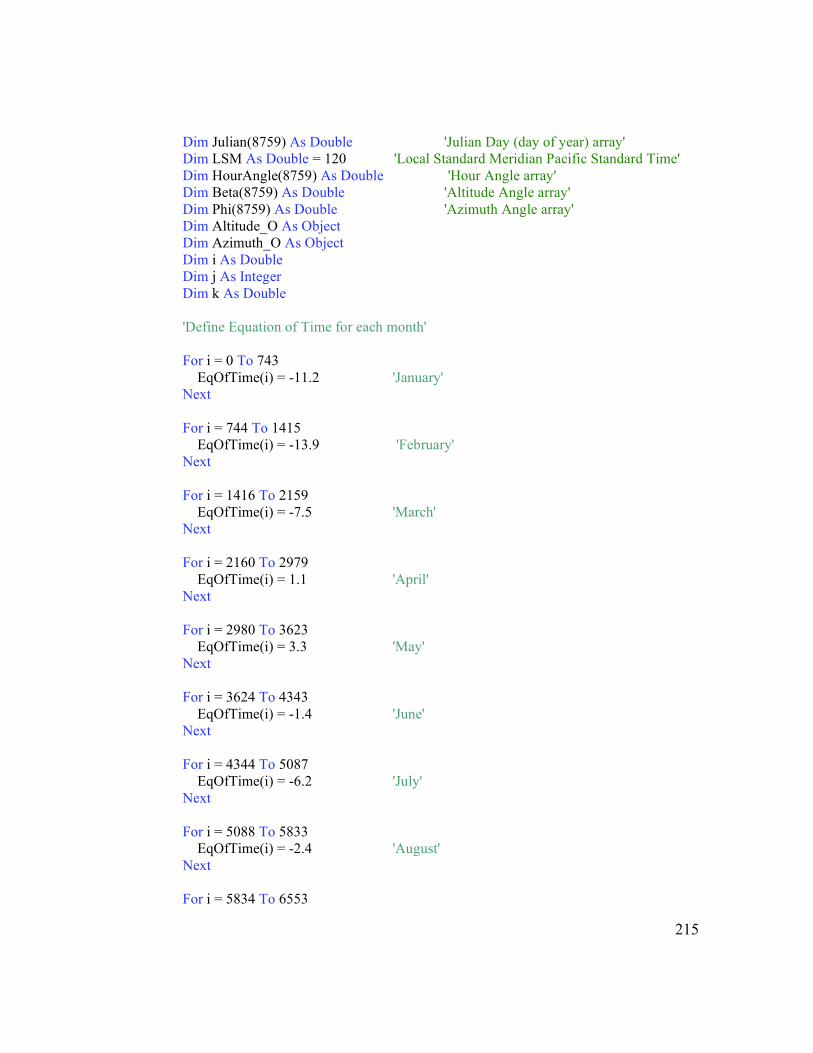
215
Dim Julian(8759) As Double 'Julian Day (day of year) array' Dim LSM As Double = 120 'Local Standard Meridian Pacific Standard Time' Dim HourAngle(8759) As Double 'Hour Angle array' Dim Beta(8759) As Double 'Altitude Angle array' Dim Phi(8759) As Double 'Azimuth Angle array' Dim Altitude_O As Object Dim Azimuth_O As Object Dim i As Double Dim j As Integer Dim k As Double 'Define Equation of Time for each month' For i = 0 To 743 EqOfTime(i) = -11.2 'January' Next For i = 744 To 1415 EqOfTime(i) = -13.9 'February' Next For i = 1416 To 2159 EqOfTime(i) = -7.5 'March' Next For i = 2160 To 2979 EqOfTime(i) = 1.1 'April' Next For i = 2980 To 3623 EqOfTime(i) = 3.3 'May' Next For i = 3624 To 4343 EqOfTime(i) = -1.4 'June' Next For i = 4344 To 5087 EqOfTime(i) = -6.2 'July' Next For i = 5088 To 5833 EqOfTime(i) = -2.4 'August' Next For i = 5834 To 6553
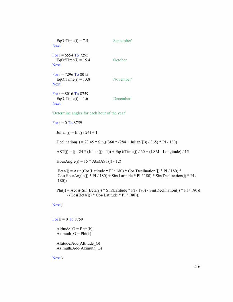
216
EqOfTime(i) = 7.5 'September' Next For i = 6554 To 7295 EqOfTime(i) = 15.4 'October' Next For i = 7296 To 8015 EqOfTime(i) = 13.8 'November' Next For i = 8016 To 8759 EqOfTime(i) = 1.6 'December' Next 'Determine angles for each hour of the year' For j = 0 To 8759 Julian(j) = Int(j / 24) + 1 Declination(j) = 23.45 * Sin(((360 * (284 + Julian(j))) / 365) * PI / 180) AST(j) = (j - 24 * (Julian(j) - 1)) + EqOfTime(j) / 60 + (LSM - Longitude) / 15 HourAngle(j) = 15 * Abs(AST(j) - 12)
Beta(j) = Asin(Cos(Latitude * PI / 180) * Cos(Declination(j) * PI / 180) * Cos(HourAngle(j) * PI / 180) + Sin(Latitude * PI / 180) * Sin(Declination(j) * PI / 180))
Phi(j) = Acos((Sin(Beta(j)) * Sin(Latitude * PI / 180) - Sin(Declination(j) * PI / 180)) / (Cos(Beta(j)) * Cos(Latitude * PI / 180))) Next j For k = 0 To 8759 Altitude_O = Beta(k) Azimuth_O = Phi(k) Altitude.Add(Altitude_O) Azimuth.Add(Azimuth_O) Next k

217
End Sub Private Sub Button1_Click(ByVal sender As System.Object, ByVal e As
System.EventArgs) Handles Button1.Click AssignCityData() SolarAngles() Form2.Show() End Sub Private Sub Button2_Click(ByVal sender As System.Object, ByVal e As System.EventArgs)
Handles Button2.Click
Form1HelpString = "Welcome to the Arbor Software. This screen welcomes you to the program and tells you what you can expect as you progress through the series of design screens. Please provide your utility rate. This can be found on your monthly electricity bill. It will be used in calculating the energy savings you can expect from planting a tree in your yard."
Form1Help.Show() Form1Help.TextBox1.Text = Form1HelpString End Sub
End Class

218
FORM 2 – BUILDING INFORMATION SCREEN
Imports System.Math Public Class Form2 Private Sub TxtBxNSWall_TextChanged (ByVal sender As System.Object, ByVal e As
System.EventArgs) Handles TxtBxNSWall.TextChanged 'Set North/South Wall variable from user input' NSWall = Val(TxtBxNSWall.Text) End Sub Private Sub TxtBxEWWall_TextChanged(ByVal sender As System.Object, ByVal e As
System.EventArgs) Handles TxtBxEWWall.TextChanged 'Set East/West Wall variable from user input' EWWall = Val(TxtBxEWWall.Text) End Sub Private Sub TxtBxFlrHt_TextChanged(ByVal sender As System.Object, ByVal e As
System.EventArgs) Handles TxtBxFlrHt.TextChanged 'Set Floor Height variable from user input' FlrHt = Val(TxtBxFlrHt.Text) End Sub Private Sub TxtBxNSWall_Validated(ByVal sender As Object, ByVal e As
System.EventArgs) Handles TxtBxNSWall.Validated Me.ErrorProvider1.SetError(TxtBxNSWall, "") End Sub Private Sub TxtNSWall_Validating(ByVal sender As Object, ByVal e As
System.ComponentModel.CancelEventArgs) Handles TxtBxNSWall.Validating
Try

219
If Me.TxtBxNSWall.Text.Length = 0 Then Me.ErrorProvider1.SetError(Me.TxtBxNSWall, "Please Enter a value") Throw New Exception("Please enter a value") ElseIf Not IsNumeric(TxtBxNSWall.Text) Then Me.ErrorProvider1.SetError(Me.TxtBxNSWall, "Please Enter a Numeric Value!") Throw New Exception("Please enter a numeric value") End If Catch ex As Exception MsgBox(ex.Message, , strTitle) End Try End Sub Private Sub TxtBxEWWall_Validated(ByVal sender As Object, ByVal e As
System.EventArgs) Handles TxtBxEWWall.Validated Me.ErrorProvider1.SetError(TxtBxEWWall, "") End Sub Private Sub TxtBxEWWall_Validating(ByVal sender As Object, ByVal e As
System.ComponentModel.CancelEventArgs) Handles TxtBxEWWall.Validating
Try If Me.TxtBxEWWall.Text.Length = 0 Then Me.ErrorProvider1.SetError(Me.TxtBxEWWall, "Please Enter a value") Throw New Exception("Please enter a value") ElseIf Not IsNumeric(TxtBxEWWall.Text) Then Me.ErrorProvider1.SetError(Me.TxtBxEWWall, "Please Enter a Numeric Value!") Throw New Exception("Please enter a numeric value") End If Catch ex As Exception MsgBox(ex.Message, , strTitle) End Try End Sub Private Sub TxtBxFlrHt_Validated(ByVal sender As Object, ByVal e As
System.EventArgs) Handles TxtBxFlrHt.Validated Me.ErrorProvider1.SetError(TxtBxFlrHt, "")

220
End Sub Private Sub TxtBxFlrHt_Validating(ByVal sender As Object, ByVal e As
System.ComponentModel.CancelEventArgs) Handles TxtBxFlrHt.Validating
Try If Me.TxtBxFlrHt.Text.Length = 0 Then Me.ErrorProvider1.SetError(Me.TxtBxFlrHt, "Please Enter a value") Throw New Exception("Please enter a value") ElseIf Not IsNumeric(TxtBxFlrHt.Text) Then Me.ErrorProvider1.SetError(Me.TxtBxFlrHt, "Please Enter a Numeric Value!") Throw New Exception("Please enter a numeric value") End If Catch ex As Exception MsgBox(ex.Message, , strTitle) End Try End Sub Private Sub Button1_Click(ByVal sender As System.Object, ByVal e As
System.EventArgs) Handles Button1.Click Form3.Show() Me.Hide() End Sub Private Sub Button2_Click(ByVal sender As System.Object, ByVal e As
System.EventArgs) Handles Button2.Click Form1.Show() Me.Hide() End Sub Private Sub Button3_Click(ByVal sender As System.Object, ByVal e As
System.EventArgs) Handles Button3.Click Form2HelpString = "This screen requires you to input information regarding the
dimensions of your house as well as your yard. The program assumes your house is a rectangle, with North and South walls

221
having the same dimension and East and West walls having the same dimension. These dimensions are used by the program to correctly place windows on your walls. If your house has slightly different wall dimensions, please provide an average length. The program also assumes that your house is oriented directly South. Please approximate the directions of your walls. The Floor Height is the height of one of your floors; it is typically around 9 feet. The yard dimensions are also required by the program for error checking. These are simply the distance between the very edge of your yard, to the corresponding wall face."
Form2Help.Show() Form2Help.TextBox1.Text = Form2HelpString End Sub End Class

222
FORM 3 – EAST WALL FENESTRATION SCREEN
Imports System.Math Public Class Form3 Private Sub TxtBxSthDist_TextChanged(ByVal sender As System.Object, ByVal e As
System.EventArgs) Handles TxtBxSthDist.TextChanged ESouthDist = Val(TxtBxSthDist.Text) End Sub Private Sub TxtBxGrndDist_TextChanged(ByVal sender As System.Object, ByVal e As
System.EventArgs) Handles TxtBxGrndDist.TextChanged EGroundDist = Val(TxtBxGrndDist.Text) End Sub Private Sub TxtBxWinWidth_TextChanged(ByVal sender As System.Object, ByVal e As
System.EventArgs) Handles TxtBxWinWidth.TextChanged EWinWidth = Val(TxtBxWinWidth.Text) End Sub Private Sub TxtBxWinHeight_TextChanged(ByVal sender As System.Object, ByVal e As
System.EventArgs) Handles TxtBxWinHeight.TextChanged EWinHeight = Val(TxtBxWinHeight.Text) End Sub Private Sub TxtBxSthDist_Validated(ByVal sender As Object, ByVal e As
System.EventArgs) Handles TxtBxSthDist.Validated Me.ErrorProvider1.SetError(TxtBxSthDist, "") End Sub

223
Private Sub TxtBxSthDist_Validating(ByVal sender As Object, ByVal e As
System.ComponentModel.CancelEventArgs) Handles TxtBxSthDist.Validating
Try If Me.TxtBxSthDist.Text.Length = 0 Then Me.ErrorProvider1.SetError(Me.TxtBxSthDist, "Please Enter a value") Throw New Exception("Please enter a value") ElseIf Not IsNumeric(TxtBxSthDist.Text) Then Me.ErrorProvider1.SetError(Me.TxtBxSthDist, "Please Enter a Numeric Value!") Throw New Exception("Please enter a numeric value") End If Catch ex As Exception MsgBox(ex.Message, , strTitle) End Try End Sub Private Sub TxtBxGrndDist_Validated(ByVal sender As Object, ByVal e As
System.EventArgs) Handles TxtBxGrndDist.Validated Me.ErrorProvider1.SetError(TxtBxGrndDist, "") End Sub Private Sub TxtBxGrndDist_Validating(ByVal sender As Object, ByVal e As
System.ComponentModel.CancelEventArgs) Handles TxtBxGrndDist.Validating
Try If Me.TxtBxGrndDist.Text.Length = 0 Then Me.ErrorProvider1.SetError(Me.TxtBxGrndDist, "Please Enter a value") Throw New Exception("Please enter a value") ElseIf Not IsNumeric(TxtBxGrndDist.Text) Then Me.ErrorProvider1.SetError(Me.TxtBxGrndDist, "Please Enter a Numeric
Value!") Throw New Exception("Please enter a numeric value") End If Catch ex As Exception MsgBox(ex.Message, , strTitle) End Try End Sub

224
Private Sub TxtBxWinWidth_Validated(ByVal sender As Object, ByVal e As
System.EventArgs) Handles TxtBxWinWidth.Validated Me.ErrorProvider1.SetError(TxtBxWinWidth, "") End Sub Private Sub TxtBxWinWidth_Validating(ByVal sender As Object, ByVal e As
System.ComponentModel.CancelEventArgs) Handles TxtBxWinWidth.Validating
Try If Me.TxtBxWinWidth.Text.Length = 0 Then Me.ErrorProvider1.SetError(Me.TxtBxWinWidth, "Please Enter a value") Throw New Exception("Please enter a value") ElseIf Not IsNumeric(TxtBxWinWidth.Text) Then Me.ErrorProvider1.SetError(Me.TxtBxWinWidth, "Please Enter a Numeric
Value!") Throw New Exception("Please enter a numeric value") End If Catch ex As Exception MsgBox(ex.Message, , strTitle) End Try End Sub Private Sub TxtBxWinHeight_Validated(ByVal sender As Object, ByVal e As
System.EventArgs) Handles TxtBxWinHeight.Validated Me.ErrorProvider1.SetError(TxtBxWinHeight, "") End Sub Private Sub TxtBxWinHeight_Validating(ByVal sender As Object, ByVal e As
System.ComponentModel.CancelEventArgs) Handles TxtBxWinHeight.Validating
Try If Me.TxtBxWinHeight.Text.Length = 0 Then Me.ErrorProvider1.SetError(Me.TxtBxWinHeight, "Please Enter a value") Throw New Exception("Please enter a value") ElseIf Not IsNumeric(TxtBxWinHeight.Text) Then

225
Me.ErrorProvider1.SetError(Me.TxtBxWinHeight, "Please Enter a Numeric Value!")
Throw New Exception("Please enter a numeric value") End If Catch ex As Exception MsgBox(ex.Message, , strTitle) End Try End Sub Private Sub AssignEastWinCoordinates() 'Assign values to East Window Point 1' EastWinArray(0, 0) = (NSWall / 2) EastWinArray(0, 1) = -(EWWall / 2) + ESouthDist EastWinArray(0, 2) = EGroundDist 'Assign values to East Window Point 2' EastWinArray(1, 0) = (NSWall / 2) EastWinArray(1, 1) = -(EWWall / 2) + ESouthDist EastWinArray(1, 2) = EGroundDist + EWinHeight 'Assign values to East Window Point 3' EastWinArray(2, 0) = (NSWall / 2) EastWinArray(2, 1) = -(EWWall / 2) + ESouthDist + EWinWidth EastWinArray(2, 2) = EGroundDist + EWinHeight 'Assign values to East Window Point 4' EastWinArray(3, 0) = (NSWall / 2) EastWinArray(3, 1) = -(EWWall / 2) + ESouthDist + EWinWidth EastWinArray(3, 2) = EGroundDist End Sub Private Sub SetEFenestration() 'Set Fenestration U-Value and SHGC' If LstBxFrame.SelectedIndex = 0 Then If LstBxGlaze.SelectedIndex = 0 Then EUFen = 0.89 ESHGC = 0.64 ElseIf LstBxGlaze.SelectedIndex = 1 Then EUFen = 0.51

226
ESHGC = 0.52 ElseIf LstBxGlaze.SelectedIndex = 2 Then EUFen = 0.4 ESHGC = 0.42 ElseIf LstBxGlaze.SelectedIndex = 3 Then EUFen = 0.39 ESHGC = 0.28 ElseIf LstBxGlaze.SelectedIndex = 4 Then EUFen = 0.36 ESHGC = 0.28 ElseIf LstBxGlaze.SelectedIndex = 5 Then EUFen = 0.51 ESHGC = 0.38 ElseIf LstBxGlaze.SelectedIndex = 6 Then EUFen = 0.4 ESHGC = 0.3 ElseIf LstBxGlaze.SelectedIndex = 7 Then EUFen = 0.39 ESHGC = 0.21 ElseIf LstBxGlaze.SelectedIndex = 8 Then EUFen = 0.51 ESHGC = 0.13 ElseIf LstBxGlaze.SelectedIndex = 9 Then EUFen = 0.39 ESHGC = 0.46 End If ElseIf LstBxFrame.SelectedIndex = 1 Then If LstBxGlaze.SelectedIndex = 0 Then EUFen = 1.27 ESHGC = 0.75 ElseIf LstBxGlaze.SelectedIndex = 1 Then EUFen = 0.81 ESHGC = 0.61 ElseIf LstBxGlaze.SelectedIndex = 2 Then EUFen = 0.69 ESHGC = 0.5 ElseIf LstBxGlaze.SelectedIndex = 3 Then EUFen = 0.67 ESHGC = 0.34 ElseIf LstBxGlaze.SelectedIndex = 4 Then EUFen = 0.63 ESHGC = 0.34 ElseIf LstBxGlaze.SelectedIndex = 5 Then EUFen = 0.81 ESHGC = 0.45

227
ElseIf LstBxGlaze.SelectedIndex = 6 Then EUFen = 0.69 ESHGC = 0.39 ElseIf LstBxGlaze.SelectedIndex = 7 Then EUFen = 0.67 ESHGC = 0.25 ElseIf LstBxGlaze.SelectedIndex = 8 Then EUFen = 0.81 ESHGC = 0.16 ElseIf LstBxGlaze.SelectedIndex = 9 Then EUFen = 0.67 ESHGC = 0.54 End If End If End Sub Private Sub Button1_Click(ByVal sender As System.Object, ByVal e As
System.EventArgs) Handles Button1.Click AssignEastWinCoordinates() SetEFenestration() Form4.Show() Me.Hide() End Sub Private Sub Button2_Click(ByVal sender As System.Object, ByVal e As
System.EventArgs) Handles Button2.Click Form2.Show() Me.Hide() End Sub Private Sub Button3_Click(ByVal sender As System.Object, ByVal e As
System.EventArgs) Handles Button3.Click Form3HelpString = "This screen prompts you to input information regarding
fenestration (or windows) on your East-facing wall. Please provide all dimensions in feet. The distance from the South wall is the distance, in feet, from the edge of the East wall that

228
intersects the South wall to the closest edge of your window. This dimension is used in placing your window. The distance from the ground is the distance from the intersection of your wall and the ground to the bottom, or sill, of your window. You are also required to input information on the window consruction. You can select either a wood/vinyl or aluminum frame, and pair it with a range of glazing types. If you are unsure of your glass type, you can probably guess based on the age of your windows. Older windows are usually single glazing, newer windows are double glazed and often have a gas filling. Many windows manufactured today also have coatings on the glass. If you are unsure, select clear double pane."
Form3Help.Show() Form3Help.TextBox1.Text = Form3HelpString End Sub End Class

229
FORM 4 – SOUTH WALL FENESTRATION SCREEN
Imports System.Math Public Class Form4 Private Sub TxtBxWstDist_TextChanged(ByVal sender As System.Object, ByVal e As
System.EventArgs) Handles TxtBxWstDist.TextChanged SWestDist = Val(TxtBxWstDist.Text) End Sub Private Sub TxtBxGrndDistS_TextChanged(ByVal sender As System.Object, ByVal e As
System.EventArgs) Handles TxtBxGrndDistS.TextChanged SGroundDist = Val(TxtBxGrndDistS.Text) End Sub Private Sub TxtBxEWinWidth_TextChanged(ByVal sender As System.Object, ByVal e
As System.EventArgs) Handles TxtBxWinWidth.TextChanged SWinWidth = Val(TxtBxWinWidth.Text) End Sub Private Sub TxtBxEWinHeight_TextChanged(ByVal sender As System.Object, ByVal e
As System.EventArgs) Handles TxtBxWinHeight.TextChanged SWinHeight = Val(TxtBxWinHeight.Text) End Sub Private Sub TxtBxWstDist_Validated(ByVal sender As Object, ByVal e As
System.EventArgs) Handles TxtBxWstDist.Validated Me.ErrorProvider1.SetError(TxtBxWstDist, "") End Sub

230
Private Sub TxtBxWstDist_Validating(ByVal sender As Object, ByVal e As
System.ComponentModel.CancelEventArgs) Handles TxtBxWstDist.Validating
Try If Me.TxtBxWstDist.Text.Length = 0 Then Me.ErrorProvider1.SetError(Me.TxtBxWstDist, "Please Enter a value") Throw New Exception("Please enter a value") ElseIf Not IsNumeric(TxtBxWstDist.Text) Then Me.ErrorProvider1.SetError(Me.TxtBxWstDist, "Please Enter a Numeric Value!") Throw New Exception("Please enter a numeric value") End If Catch ex As Exception MsgBox(ex.Message, , strTitle) End Try End Sub Private Sub TxtBxGrndDistS_Validated(ByVal sender As Object, ByVal e As
System.EventArgs) Handles TxtBxGrndDistS.Validated Me.ErrorProvider1.SetError(TxtBxGrndDistS, "") End Sub Private Sub TxtBxGrndDistS_Validating(ByVal sender As Object, ByVal e As
System.ComponentModel.CancelEventArgs) Handles TxtBxGrndDistS.Validating
Try If Me.TxtBxGrndDistS.Text.Length = 0 Then Me.ErrorProvider1.SetError(Me.TxtBxGrndDistS, "Please Enter a value") Throw New Exception("Please enter a value") ElseIf Not IsNumeric(TxtBxGrndDistS.Text) Then Me.ErrorProvider1.SetError(Me.TxtBxGrndDistS, "Please Enter a Numeric
Value!") Throw New Exception("Please enter a numeric value") End If Catch ex As Exception MsgBox(ex.Message, , strTitle) End Try

231
End Sub Private Sub TxtBxWinWidth_Validated(ByVal sender As Object, ByVal e As
System.EventArgs) Handles TxtBxWinWidth.Validated Me.ErrorProvider1.SetError(TxtBxWinWidth, "") End Sub Private Sub TxtBxWinWidth_Validating(ByVal sender As Object, ByVal e As
System.ComponentModel.CancelEventArgs) Handles TxtBxWinWidth.Validating
Try If Me.TxtBxWinWidth.Text.Length = 0 Then Me.ErrorProvider1.SetError(Me.TxtBxWinWidth, "Please Enter a value") Throw New Exception("Please enter a value") ElseIf Not IsNumeric(TxtBxWinWidth.Text) Then Me.ErrorProvider1.SetError(Me.TxtBxWinWidth, "Please Enter a Numeric
Value!") Throw New Exception("Please enter a numeric value") End If Catch ex As Exception MsgBox(ex.Message, , strTitle) End Try End Sub Private Sub TxtBxWinHeight_Validated(ByVal sender As Object, ByVal e As
System.EventArgs) Handles TxtBxWinHeight.Validated Me.ErrorProvider1.SetError(TxtBxWinHeight, "") End Sub Private Sub TxtBxWinHeight_Validating(ByVal sender As Object, ByVal e As
System.ComponentModel.CancelEventArgs) Handles TxtBxWinHeight.Validating
Try If Me.TxtBxWinHeight.Text.Length = 0 Then Me.ErrorProvider1.SetError(Me.TxtBxWinHeight, "Please Enter a value") Throw New Exception("Please enter a value")

232
ElseIf Not IsNumeric(TxtBxWinHeight.Text) Then Me.ErrorProvider1.SetError(Me.TxtBxWinHeight, "Please Enter a Numeric
Value!") Throw New Exception("Please enter a numeric value") End If Catch ex As Exception MsgBox(ex.Message, , strTitle) End Try End Sub Private Sub AssignSouthWinCoordinates() 'Assign values to South Window Point 1' SouthWinArray(0, 0) = -(NSWall / 2) + SWestDist SouthWinArray(0, 1) = -(EWWall / 2) SouthWinArray(0, 2) = SGroundDist 'Assign values to South Window Point 2' SouthWinArray(1, 0) = -(NSWall / 2) + SWestDist SouthWinArray(1, 1) = -(EWWall / 2) SouthWinArray(1, 2) = SGroundDist + SWinHeight 'Assign values to South Window Point 3' SouthWinArray(2, 0) = -(NSWall / 2) + SWestDist + SWinWidth SouthWinArray(2, 1) = -(EWWall / 2) SouthWinArray(2, 2) = SGroundDist + SWinHeight 'Assign values to South Window Point 4' SouthWinArray(3, 0) = -(NSWall / 2) + SWestDist + SWinWidth SouthWinArray(3, 1) = -(EWWall / 2) SouthWinArray(3, 2) = SGroundDist End Sub Private Sub SetSFenestration() 'Set Fenestration U-Value and SHGC' If LstBxFrame.SelectedIndex = 0 Then If LstBxGlaze.SelectedIndex = 0 Then SUFen = 0.89 SSHGC = 0.64 ElseIf LstBxGlaze.SelectedIndex = 1 Then

233
SUFen = 0.51 SSHGC = 0.52 ElseIf LstBxGlaze.SelectedIndex = 2 Then SUFen = 0.4 SSHGC = 0.42 ElseIf LstBxGlaze.SelectedIndex = 3 Then SUFen = 0.39 SSHGC = 0.28 ElseIf LstBxGlaze.SelectedIndex = 4 Then SUFen = 0.36 SSHGC = 0.28 ElseIf LstBxGlaze.SelectedIndex = 5 Then SUFen = 0.51 SSHGC = 0.38 ElseIf LstBxGlaze.SelectedIndex = 6 Then SUFen = 0.4 SSHGC = 0.3 ElseIf LstBxGlaze.SelectedIndex = 7 Then SUFen = 0.39 SSHGC = 0.21 ElseIf LstBxGlaze.SelectedIndex = 8 Then SUFen = 0.51 SSHGC = 0.13 ElseIf LstBxGlaze.SelectedIndex = 9 Then SUFen = 0.39 SSHGC = 0.46 End If ElseIf LstBxFrame.SelectedIndex = 1 Then If LstBxGlaze.SelectedIndex = 0 Then SUFen = 1.27 SSHGC = 0.75 ElseIf LstBxGlaze.SelectedIndex = 1 Then SUFen = 0.81 SSHGC = 0.61 ElseIf LstBxGlaze.SelectedIndex = 2 Then SUFen = 0.69 SSHGC = 0.5 ElseIf LstBxGlaze.SelectedIndex = 3 Then SUFen = 0.67 SSHGC = 0.34 ElseIf LstBxGlaze.SelectedIndex = 4 Then SUFen = 0.63 SSHGC = 0.34 ElseIf LstBxGlaze.SelectedIndex = 5 Then SUFen = 0.81

234
SSHGC = 0.45 ElseIf LstBxGlaze.SelectedIndex = 6 Then SUFen = 0.69 SSHGC = 0.39 ElseIf LstBxGlaze.SelectedIndex = 7 Then SUFen = 0.67 SSHGC = 0.25 ElseIf LstBxGlaze.SelectedIndex = 8 Then SUFen = 0.81 SSHGC = 0.16 ElseIf LstBxGlaze.SelectedIndex = 9 Then SUFen = 0.67 SSHGC = 0.54 End If End If End Sub Private Sub Button1_Click(ByVal sender As System.Object, ByVal e As
System.EventArgs) Handles Button1.Click AssignSouthWinCoordinates() SetSFenestration() Form5.Show() Me.Hide() End Sub Private Sub Button2_Click(ByVal sender As System.Object, ByVal e As
System.EventArgs) Handles Button2.Click Form3.Show() Me.Hide() End Sub Private Sub Button3_Click(ByVal sender As System.Object, ByVal e As
System.EventArgs) Handles Button3.Click Form4HelpString = "This screen prompts you to input information regarding
fenestration (or windows) on your South-facing wall. Please provide all dimensions in feet. The distance from the West wall

235
is the distance, in feet, from the edge of the South wall that intersects the West wall to the closest edge of your window. This dimension is used in placing your window. The distance from the ground is the distance from the intersection of your wall and the ground to the bottom, or sill, of your window. You are also required to input information on the window consruction. You can select either a wood/vinyl or aluminum frame, and pair it with a range of glazing types. If you are unsure of your glass type, you can probably guess based on the age of your windows. Older windows are usually single glazing, newer windows are double glazed and often have a gas filling. Many windows manufactured today also have coatings on the glass. If you are unsure, select clear double pane."
Form4Help.Show() Form4Help.TextBox1.Text = Form4HelpString End Sub End Class

236
FORM 5 – WEST WALL FENESTRATION SCREEN
Imports System.Math Public Class Form5 Private Sub TxtBxNrthDist_TextChanged(ByVal sender As System.Object, ByVal e As
System.EventArgs) Handles TxtBxNrthDist.TextChanged WNorthDist = Val(TxtBxNrthDist.Text) End Sub Private Sub TxtBxGrndDistW_TextChanged(ByVal sender As System.Object, ByVal e
As System.EventArgs) Handles TxtBxGrndDistW.TextChanged WGroundDist = Val(TxtBxGrndDistW.Text) End Sub Private Sub TxtBxWinWidth_TextChanged(ByVal sender As System.Object, ByVal e As
System.EventArgs) Handles TxtBxWinWidth.TextChanged WWinWidth = Val(TxtBxWinWidth.Text) End Sub Private Sub TxtBxWinHeight_TextChanged(ByVal sender As System.Object, ByVal e As
System.EventArgs) Handles TxtBxWinHeight.TextChanged WWinHeight = Val(TxtBxWinHeight.Text) End Sub Private Sub TxtBxNrthDist_Validated(ByVal sender As Object, ByVal e As
System.EventArgs) Handles TxtBxNrthDist.Validated Me.ErrorProvider1.SetError(TxtBxNrthDist, "") End Sub

237
Private Sub TxtBxNrthDist_Validating(ByVal sender As Object, ByVal e As System.ComponentModel.CancelEventArgs) Handles TxtBxNrthDist.Validating
Try If Me.TxtBxNrthDist.Text.Length = 0 Then Me.ErrorProvider1.SetError(Me.TxtBxNrthDist, "Please Enter a value") Throw New Exception("Please enter a value") ElseIf Not IsNumeric(TxtBxNrthDist.Text) Then Me.ErrorProvider1.SetError(Me.TxtBxNrthDist, "Please Enter a Numeric Value!") Throw New Exception("Please enter a numeric value") End If Catch ex As Exception MsgBox(ex.Message, , strTitle) End Try End Sub Private Sub TxtBxGrndDistW_Validated(ByVal sender As Object, ByVal e As
System.EventArgs) Handles TxtBxGrndDistW.Validated Me.ErrorProvider1.SetError(TxtBxGrndDistW, "") End Sub Private Sub TxtBxGrndDistW_Validating(ByVal sender As Object, ByVal e As
System.ComponentModel.CancelEventArgs) Handles TxtBxGrndDistW.Validating
Try If Me.TxtBxGrndDistW.Text.Length = 0 Then Me.ErrorProvider1.SetError(Me.TxtBxGrndDistW, "Please Enter a value") Throw New Exception("Please enter a value") ElseIf Not IsNumeric(TxtBxGrndDistW.Text) Then Me.ErrorProvider1.SetError(Me.TxtBxGrndDistW, "Please Enter a Numeric
Value!") Throw New Exception("Please enter a numeric value") End If Catch ex As Exception MsgBox(ex.Message, , strTitle) End Try End Sub

238
Private Sub TxtBxWinWidth_Validated(ByVal sender As Object, ByVal e As System.EventArgs) Handles TxtBxWinWidth.Validated
Me.ErrorProvider1.SetError(TxtBxWinWidth, "") End Sub Private Sub TxtBxWinWidth_Validating(ByVal sender As Object, ByVal e As
System.ComponentModel.CancelEventArgs) Handles TxtBxWinWidth.Validating
Try If Me.TxtBxWinWidth.Text.Length = 0 Then Me.ErrorProvider1.SetError(Me.TxtBxWinWidth, "Please Enter a value") Throw New Exception("Please enter a value") ElseIf Not IsNumeric(TxtBxWinWidth.Text) Then Me.ErrorProvider1.SetError(Me.TxtBxWinWidth, "Please Enter a Numeric
Value!") Throw New Exception("Please enter a numeric value") End If Catch ex As Exception MsgBox(ex.Message, , strTitle) End Try End Sub Private Sub TxtBxWinHeight_Validated(ByVal sender As Object, ByVal e As
System.EventArgs) Handles TxtBxWinHeight.Validated Me.ErrorProvider1.SetError(TxtBxWinHeight, "") End Sub Private Sub TxtBxWinHeight_Validating(ByVal sender As Object, ByVal e As
System.ComponentModel.CancelEventArgs) Handles TxtBxWinHeight.Validating
Try If Me.TxtBxWinHeight.Text.Length = 0 Then Me.ErrorProvider1.SetError(Me.TxtBxWinHeight, "Please Enter a value") Throw New Exception("Please enter a value") ElseIf Not IsNumeric(TxtBxWinHeight.Text) Then

239
Me.ErrorProvider1.SetError(Me.TxtBxWinHeight, "Please Enter a Numeric Value!")
Throw New Exception("Please enter a numeric value") End If Catch ex As Exception MsgBox(ex.Message, , strTitle) End Try End Sub Private Sub AssignWestWinCoordinates() 'Assign values to West Window Point 1' WestWinArray(0, 0) = -(NSWall / 2) WestWinArray(0, 1) = (EWWall / 2) - WNorthDist WestWinArray(0, 2) = WGroundDist 'Assign values to West Window Point 2' WestWinArray(1, 0) = -(NSWall / 2) WestWinArray(1, 1) = (EWWall / 2) - WNorthDist WestWinArray(1, 2) = WGroundDist + WWinHeight 'Assign values to West Window Point 3' WestWinArray(2, 0) = -(NSWall / 2) WestWinArray(2, 1) = (EWWall / 2) - WNorthDist - WWinWidth WestWinArray(2, 2) = WGroundDist + WWinHeight 'ASsign values to West Window Point 4' WestWinArray(3, 0) = -(NSWall / 2) WestWinArray(3, 1) = (EWWall / 2) - WNorthDist - WWinWidth WestWinArray(3, 2) = WGroundDist End Sub Private Sub SetWFenestration() 'Set Fenestration U-Value and SHGC' If LstBxFrame.SelectedIndex = 0 Then If LstBxGlaze.SelectedIndex = 0 Then WUFen = 0.89 WSHGC = 0.64 ElseIf LstBxGlaze.SelectedIndex = 1 Then WUFen = 0.51

240
WSHGC = 0.52 ElseIf LstBxGlaze.SelectedIndex = 2 Then WUFen = 0.4 WSHGC = 0.42 ElseIf LstBxGlaze.SelectedIndex = 3 Then WUFen = 0.39 WSHGC = 0.28 ElseIf LstBxGlaze.SelectedIndex = 4 Then WUFen = 0.36 WSHGC = 0.28 ElseIf LstBxGlaze.SelectedIndex = 5 Then WUFen = 0.51 WSHGC = 0.38 ElseIf LstBxGlaze.SelectedIndex = 6 Then WUFen = 0.4 WSHGC = 0.3 ElseIf LstBxGlaze.SelectedIndex = 7 Then WUFen = 0.39 WSHGC = 0.21 ElseIf LstBxGlaze.SelectedIndex = 8 Then WUFen = 0.51 WSHGC = 0.13 ElseIf LstBxGlaze.SelectedIndex = 9 Then WUFen = 0.39 WSHGC = 0.46 End If ElseIf LstBxFrame.SelectedIndex = 1 Then If LstBxGlaze.SelectedIndex = 0 Then WUFen = 1.27 WSHGC = 0.75 ElseIf LstBxGlaze.SelectedIndex = 1 Then WUFen = 0.81 WSHGC = 0.61 ElseIf LstBxGlaze.SelectedIndex = 2 Then WUFen = 0.69 WSHGC = 0.5 ElseIf LstBxGlaze.SelectedIndex = 3 Then WUFen = 0.67 WSHGC = 0.34 ElseIf LstBxGlaze.SelectedIndex = 4 Then WUFen = 0.63 WSHGC = 0.34 ElseIf LstBxGlaze.SelectedIndex = 5 Then WUFen = 0.81 WSHGC = 0.45

241
ElseIf LstBxGlaze.SelectedIndex = 6 Then WUFen = 0.69 WSHGC = 0.39 ElseIf LstBxGlaze.SelectedIndex = 7 Then WUFen = 0.67 WSHGC = 0.25 ElseIf LstBxGlaze.SelectedIndex = 8 Then WUFen = 0.81 WSHGC = 0.16 ElseIf LstBxGlaze.SelectedIndex = 9 Then WUFen = 0.67 WSHGC = 0.54 End If End If End Sub Private Sub Button1_Click(ByVal sender As System.Object, ByVal e As
System.EventArgs) Handles Button1.Click AssignWestWinCoordinates() SetWFenestration() Form6.Show() Me.Hide() End Sub Private Sub Button2_Click(ByVal sender As System.Object, ByVal e As
System.EventArgs) Handles Button2.Click Form4.Show() Me.Hide() End Sub Private Sub Button3_Click(ByVal sender As System.Object, ByVal e As
System.EventArgs) Handles Button3.Click Form5HelpString = "This screen prompts you to input information regarding
fenestration (or windows) on your West-facing wall. Please provide all dimensions in feet. The distance from the North wall is the distance, in feet, from the edge of the West wall that intersects

242
the North wall to the closest edge of your window. This dimension is used in placing your window. The distance from the ground is the distance from the intersection of your wall and the ground to the bottom, or sill, of your window. You are also required to input information on the window consruction. You can select either a wood/vinyl or aluminum frame, and pair it with a range of glazing types. If you are unsure of your glass type, you can probably guess based on the age of your windows. Older windows are usually single glazing, newer windows are double glazed and often have a gas filling. Many windows manufactured today also have coatings on the glass. If you are unsure, select clear double pane."
Form5Help.Show() Form5Help.TextBox1.Text = Form5HelpString End Sub End Class

243
FORM 6 – TREE SELECTION SCREEN
Imports System.Math Public Class Form6 Private Sub Tall_DeciduousBindingNavigatorSaveItem_Click(ByVal sender As
System.Object, ByVal e As System.EventArgs) Me.Validate() Me.Tall_DeciduousBindingSource.EndEdit() Me.TableAdapterManager.UpdateAll(Me.TreeDataDataSet) End Sub Private Sub Form6_Load(ByVal sender As System.Object, ByVal e As
System.EventArgs) Handles MyBase.Load 'TODO: This line of code loads data into the 'TreeDataDataSet.Tall_Deciduous' table.’
Me.Tall_DeciduousTableAdapter.Fill(Me.TreeDataDataSet.Tall_Deciduous) End Sub Private Sub TreeSelection() Dim i As Integer TreeData = TreeDataDataSet.Tall_Deciduous If RadBtnBigLeafMaple.Checked = True Then i = 0 End If If RadBtnBoxElder.Checked = True Then i = 1 End If If RadBtnSilkTree.Checked = True Then i = 2 End If If RadBtnModestoAsh.Checked = True Then i = 3
244
End If If RadBtnHoneyLocust.Checked = True Then i = 4 End If If RadBtnNorCalBW.Checked = True Then i = 5 End If If RadBtnChinesePist.Checked = True Then i = 6 End If If RadBtnFremontCotton.Checked = True Then i = 7 End If If RadBtnCalPear.Checked = True Then i = 8 End If If RadBtnChineseElm.Checked = True Then i = 9 End If TreeName = TreeData.Rows(i).Item(1) TreeHeight = TreeData.Rows(i).Item(3) TreeCanopyDiam = TreeData.Rows(i).Item(5) SummerTrans = TreeData.Rows(i).Item(6) WinterTrans = TreeData.Rows(i).Item(7) Foliation = TreeData.Rows(i).Item(8) Defoliation = TreeData.Rows(i).Item(9) End Sub Private Sub TreePicture() TreeData = TreeDataDataSet.Tall_Deciduous If RadBtnBigLeafMaple.Checked = True Then PictureBoxSummer.Image = Image.FromFile("C:\Trees\Tall Deciduous\Acer
macrophyllum\Acer mac summer\acer_mac_summer.jpg") PictureBoxWinter.Image = Image.FromFile("C:\Trees\Tall Deciduous\Acer
macrophyllum\Acer mac winter\acer_mac_winter.jpg")
245
TextBox1.Text = "The BigLeaf Maple has a fast growth rate, reaching 30-75 feet tall with a 30-50 foot canopy diameter. Leaves are smooth light green, with bright yellow flowers blooming in the spring. The bark is a smooth gray-brown that becomes reddish brown. Small, sharp, bristle like hairs on seed sheath covering may irriate skin. Limbs can be weak and break easily. The longevity of this tree is esimated at 50-80 years."
End If If RadBtnBoxElder.Checked = True Then PictureBoxSummer.Image = Image.FromFile("C:\Trees\Tall Deciduous\Acer
negundo\Acer neg summer\acer_neg_summer.jpg") PictureBoxWinter.Image = Image.FromFile("C:\Trees\Tall Deciduous\Acer
negundo\Acer neg winter\acer_neg_winter.jpg") TextBox1.Text = "The Box Elder has an initially fast growth rate that slows. At
maturity this tree will reach 20-50 feet tall, with a canopy diameter equal in size to it's height. Leaves are a dull yellowish green, and small, yellowish green flowers bloom in the spring. The bark is a thin, pale grayish brown that becomes darker with age. This tree can suffer from breakage since wood can be weak. The longevity of this tree is esimated at 30-50 years."
End If If RadBtnCalPear.Checked = True Then PictureBoxSummer.Image = Image.FromFile("C:\Trees\Tall Deciduous\Pyrus
calleryana\Pyrus summer\pyrus_summer.jpg") PictureBoxWinter.Image = Image.FromFile("C:\Trees\Tall Deciduous\Pyrus
calleryana\Pyrus winter\pyrus_winter.jpg") TextBox1.Text = "The Bradford Pear has a fast growth rate, reaching 50 feet tall with
a 30 foot canopy diameter. Leaves are dark green, turning deep scarlet-range or wide red in the fall. Clusters of heavily fragrant, white, wide-petaled flowers emerge early in spring. The bark is smooth, grayish brown becoming shallowly fissured with age. The tree is often used as a shade tree and is most effective planted in groves or in rows. The longevity of this tree is esimated at 70-80 years."
End If If RadBtnChineseElm.Checked = True Then PictureBoxSummer.Image = Image.FromFile("C:\Trees\Tall Deciduous\Ulmus
parvifolia\Ulmus summer\ulmus_summer.jpg") PictureBoxWinter.Image = Image.FromFile("C:\Trees\Tall Deciduous\Ulmus
parvifolia\Ulmus winter\ulmus_winter.jpg") TextBox1.Text = "The Chinese Elm has a very fast growth rate, reaching 40-60 feet
tall with a 50-70 foot canopy diameter. Leaves are a dark green, turning yellow to reddish orange in the fall. Tiny yellow-green
246
flowers occur in the fall. The bark is a smooth, light brown with thin, flaky scales. The tree is used widely as a shade tree and maintains most of its foliage through mild winters. The longevity of this tree is esimated at 100 years or more."
End If If RadBtnChinesePist.Checked = True Then PictureBoxSummer.Image = Image.FromFile("C:\Trees\Tall Deciduous\Pistacia
chinensis\Pistacia summer\pistacia_summer.jpg") PictureBoxWinter.Image = Image.FromFile("C:\Trees\Tall Deciduous\Pistacia
chinensis\Pistacia winter\pistacia_winter.jpg") TextBox1.Text = "The Chinese Pistache has a slow to moderate growth rate,
reaching 30-60 feet tall with a canopy diameter equal in size. Leaves are a dark to medium green, turning bright orange to deep red or bright yellow in the fall. Female trees produce clusers of small, reddish drupe fruits favored by birds. The bark is reddish brown and becomes gray-brown and finely fissured. This tree is a popular street or shade tree, favored for it's round canopy and bright fall color. The longevity of this tree is esimated at 80-100 years."
End If If RadBtnFremontCotton.Checked = True Then PictureBoxSummer.Image = Image.FromFile("C:\Trees\Tall Deciduous\Populus
fremontii\Populus summer\populus_summer.jpg") PictureBoxWinter.Image = Image.FromFile("C:\Trees\Tall Deciduous\Populus
fremontii\Populus winter\populus_winter.jpg") TextBox1.Text = "The Fremont Cottonwood has a very fast growth rate, reaching 40-
60 feet tall with a 30 foot canopy diameter. Leaves are a dark green, turning a bright to dull yellow or light orange in the fall. The bark is a pale, ashy brown that becomes dark grayish brown and deeply furrowed. Flowers are yellowish green catskins, appearing before leaves in the spring. The wood of this tree is relatively weak, with infasive surface roots that may suffer if nicked. The longevity of this tree is estimated at 75-100 years."
End If If RadBtnHoneyLocust.Checked = True Then PictureBoxSummer.Image = Image.FromFile("C:\Trees\Tall Deciduous\Gleditsia
triacanthos\Gleditsia summer\gleditsia_summer.jpg") PictureBoxWinter.Image = Image.FromFile("C:\Trees\Tall Deciduous\Gleditsia
triacanthos\Gleditsia winter\gleditsia_winter.jpg") TextBox1.Text = "The Thornless Honey Locust has a fast growth rate, reaching 35-
70 feet tall with a 25-35 foot canopy diameter. Leaves are light green with a light yellow fall color. Bark is a grayish brown with long, shallow fissures and scaly or plated ridges. This tree is
247
commonly used as a shade tree but is slow to leaf in the spring and dropes leaves earily in the fall. The longevity of this tree is esimated at 50-100 years."
End If If RadBtnModestoAsh.Checked = True Then PictureBoxSummer.Image = Image.FromFile("C:\Trees\Tall Deciduous\Fraxinus
velutina\Fraxinus summer\fraxinus_summer.jpg") PictureBoxWinter.Image = Image.FromFile("C:\Trees\Tall Deciduous\Fraxinus
velutina\Fraxinus winter\fraxinus_winter.jpg") TextBox1.Text = "The Modesto Ash has a fast growth rate, raching 50 feet tall with a
30 foot canopy diameter. Leaves can be medium green as well as bright yellow. The bark is a thin and gray and develops shallow, reddish brown fissures with scaly gray ridges. This tree is often used as a shade tree, but can be succesptible to disease. The longevity of this tree is estimated at 60-80 years."
End If If RadBtnNorCalBW.Checked = True Then PictureBoxSummer.Image = Image.FromFile("C:\Trees\Tall Deciduous\Juglans
hindsii\Juglans summer\juglans_summer.jpg") PictureBoxWinter.Image = Image.FromFile("C:\Trees\Tall Deciduous\Juglans
hindsii\Juglans winter\juglans_winter.jpg") TextBox1.Text = "The Northern California Black Walnut has a slow growth rate,
reaching 30-50 feet tall with a canopy diameter equal in size. Leaves are a light yellow green and produces thinly husked gren fruit that mature in late summer. The bark is a thin and ashy color that becomes blackish brown and deeply furrowed with age. This tree requires well-drained soils and is quite drought tolerant. The longevity of this tree is esimated at 50-75 years."
End If If RadBtnSilkTree.Checked = True Then PictureBoxSummer.Image = Image.FromFile("C:\Trees\Tall Deciduous\Albizia
julibrissin\Albizia summer\albizia_summer.jpg") PictureBoxWinter.Image = Image.FromFile("C:\Trees\Tall Deciduous\Albizia
julibrissin\Albizia winter\albizia_winter.jpg") TextBox1.Text = "The Silk Tree has a moderate growth rate, reaching a height of 40
feet with a canopy diameter twice its height. Leaves have a yellow to reddish fall color, and pink to reddish, many-stamened flowers occur during midsummer. The bark is a smooth, grayish yellow that can become fissured with age. This tree does well in summer heat and tolerates drought when established. The longevity of this tree is estaimated at 75-125 years."
End If

248
End Sub Private Sub BtnSelectTree_Click(ByVal sender As System.Object, ByVal e As
System.EventArgs) Handles BtnSelectTree.Click TreePicture() PictureBoxSummer.Visible = True PictureBoxWinter.Visible = True TextBox1.Visible = True BtnNoTree.Visible = True BtnYesTree.Visible = True End Sub Private Sub Button1_Click(ByVal sender As System.Object, ByVal e As
System.EventArgs) Handles Button1.Click Form5.Show() Me.Hide() End Sub Private Sub BtnNoTree_Click(ByVal sender As System.Object, ByVal e As
System.EventArgs) Handles BtnNoTree.Click BtnNoTree.Visible = False BtnYesTree.Visible = False PictureBoxSummer.Visible = False PictureBoxWinter.Visible = False TextBox1.Visible = False End Sub Private Sub BtnYesTree_Click(ByVal sender As System.Object, ByVal e As
System.EventArgs) Handles BtnYesTree.Click TreeSelection() Form7.Show() Me.Hide()

249
End Sub Private Sub Button2_Click(ByVal sender As System.Object, ByVal e As System.EventArgs) Handles Button2.Click Form6HelpString = "This screen is the tree selection screen. You are provided with a
list of trees that are either native to Southern California or well adapted to it's climate. Please click on a tree you think you might like, and then click the 'Select Tree' button. You will then be shown two pictures of the tree and provided with further information on the tree, including leaf, flower, and bark color, as well as life span and any special features. If you like the tree, click the 'Yes, I like this tree' button. Clicking this button will take you to the next screen. If you wish to view another tree, click the 'No, I don't like this tree' button."
Form6Help.Show() Form6Help.TextBox1.Text = Form6HelpString End Sub End Class

250
FORM 7 – TREE PLACEMENT SCREEN Imports System.Math Public Class Form7 Private Sub TxtBxTreeX_TextChanged(ByVal sender As System.Object, ByVal e As
System.EventArgs) Handles TxtBxTreeX.TextChanged TreeX = Val(TxtBxTreeX.Text) End Sub Private Sub TxtBxTreeY_TextChanged(ByVal sender As System.Object, ByVal e As
System.EventArgs) Handles TxtBxTreeY.TextChanged TreeY = Val(TxtBxTreeY.Text) End Sub Private Sub TxtBxBranchHeight_TextChanged(ByVal sender As System.Object, ByVal e
As System.EventArgs) Handles TxtBxBranchHeight.TextChanged BranchHeight = Val(TxtBxBranchHeight.Text) End Sub Private Sub TxtBxTreeX_Validated(ByVal sender As Object, ByVal e As
System.EventArgs) Handles TxtBxTreeX.Validated Me.ErrorProvider1.SetError(TxtBxTreeX, "") End Sub Private Sub TxtBxTreeX_Validating(ByVal sender As Object, ByVal e As
System.ComponentModel.CancelEventArgs) Handles TxtBxTreeX.Validating
Try If Me.TxtBxTreeX.Text.Length = 0 Then Me.ErrorProvider1.SetError(Me.TxtBxTreeX, "Please Enter a value") Throw New Exception("Please enter a value")

251
ElseIf Not IsNumeric(TxtBxTreeX.Text) Then Me.ErrorProvider1.SetError(Me.TxtBxTreeX, "Please Enter a Numeric Value!") Throw New Exception("Please enter a numeric value") End If Catch ex As Exception MsgBox(ex.Message, , strTitle) End Try End Sub Private Sub TxtBxTreeY_Validated(ByVal sender As Object, ByVal e As
System.EventArgs) Handles TxtBxTreeY.Validated Me.ErrorProvider1.SetError(TxtBxTreeY, "") End Sub Private Sub TxtBxTreeY_Validating(ByVal sender As Object, ByVal e As
System.ComponentModel.CancelEventArgs) Handles TxtBxTreeY.Validating
Try If Me.TxtBxTreeY.Text.Length = 0 Then Me.ErrorProvider1.SetError(Me.TxtBxTreeY, "Please Enter a value") Throw New Exception("Please enter a value") ElseIf Not IsNumeric(TxtBxTreeY.Text) Then Me.ErrorProvider1.SetError(Me.TxtBxTreeY, "Please Enter a Numeric Value!") Throw New Exception("Please enter a numeric value") End If Catch ex As Exception MsgBox(ex.Message, , strTitle) End Try End Sub Private Sub TxtBxBranchHeight_Validated(ByVal sender As Object, ByVal e As
System.EventArgs) Handles TxtBxBranchHeight.Validated Me.ErrorProvider1.SetError(TxtBxBranchHeight, "") End Sub
252
Private Sub TxtBxBranchHeight_Validating(ByVal sender As Object, ByVal e As System.ComponentModel.CancelEventArgs) Handles TxtBxBranchHeight.Validating
Try If Me.TxtBxBranchHeight.Text.Length = 0 Then Me.ErrorProvider1.SetError(Me.TxtBxBranchHeight, "Please Enter a value") Throw New Exception("Please enter a value") ElseIf Not IsNumeric(TxtBxBranchHeight.Text) Then Me.ErrorProvider1.SetError(Me.TxtBxBranchHeight, "Please Enter a Numeric
Value!") Throw New Exception("Please enter a numeric value") End If Catch ex As Exception MsgBox(ex.Message, , strTitle) End Try End Sub Private Sub AssignSouthTreeArray() TreeRadius = TreeCanopyDiam / 2 'Assign P1 points' SouthTreeArray(0, 0) = TreeX SouthTreeArray(0, 1) = TreeY SouthTreeArray(0, 2) = 0 'Assign P2 points' SouthTreeArray(1, 0) = TreeX SouthTreeArray(1, 1) = TreeY SouthTreeArray(1, 2) = BranchHeight 'Assign P3 points' SouthTreeArray(2, 0) = TreeX - TreeRadius SouthTreeArray(2, 1) = TreeY SouthTreeArray(2, 2) = BranchHeight 'Assign P4 points at 175 degrees' SouthTreeArray(3, 0) = TreeX + TreeRadius * Cos(3.054) SouthTreeArray(3, 1) = TreeY SouthTreeArray(3, 2) = BranchHeight + TreeRadius * Sin(3.054) 'Assign P5 points at 170 degrees' SouthTreeArray(4, 0) = TreeX + TreeRadius * Cos(2.967)

253
SouthTreeArray(4, 1) = TreeY SouthTreeArray(4, 2) = BranchHeight + TreeRadius * Sin(2.967) 'Assign P6 points at 165 degrees' SouthTreeArray(5, 0) = TreeX + TreeRadius * Cos(2.88) SouthTreeArray(5, 1) = TreeY SouthTreeArray(5, 2) = BranchHeight + TreeRadius * Sin(2.88) 'Assign P7 points at 160 degrees' SouthTreeArray(6, 0) = TreeX + TreeRadius * Cos(2.792) SouthTreeArray(6, 1) = TreeY SouthTreeArray(6, 2) = BranchHeight + TreeRadius * Sin(2.792) 'Assign P8 points at 155 degrees' SouthTreeArray(7, 0) = TreeX + TreeRadius * Cos(2.705) SouthTreeArray(7, 1) = TreeY SouthTreeArray(7, 2) = BranchHeight + TreeRadius * Sin(2.705) 'Assign P9 points at 150 degrees' SouthTreeArray(8, 0) = TreeX + TreeRadius * Cos(2.618) SouthTreeArray(8, 1) = TreeY SouthTreeArray(8, 2) = BranchHeight + TreeRadius * Sin(2.618) 'Assign P10 points at 145 degrees' SouthTreeArray(9, 0) = TreeX + TreeRadius * Cos(2.531) SouthTreeArray(9, 1) = TreeY SouthTreeArray(9, 2) = BranchHeight + TreeRadius * Sin(2.531) 'Assign P11 points at 140 degrees' SouthTreeArray(10, 0) = TreeX + TreeRadius * Cos(2.443) SouthTreeArray(10, 1) = TreeY SouthTreeArray(10, 2) = BranchHeight + TreeRadius * Sin(2.443) 'Assign P12 points at 135 degrees' SouthTreeArray(11, 0) = TreeX + TreeRadius * Cos(2.356) SouthTreeArray(11, 1) = TreeY SouthTreeArray(11, 2) = BranchHeight + TreeRadius * Sin(2.356) 'Assign P13 points at 130 degrees' SouthTreeArray(12, 0) = TreeX + TreeRadius * Cos(2.269) SouthTreeArray(12, 1) = TreeY SouthTreeArray(12, 2) = BranchHeight + TreeRadius * Sin(2.269) 'Assign P14 at 125 degrees' SouthTreeArray(13, 0) = TreeX + TreeRadius * Cos(2.182) SouthTreeArray(13, 1) = TreeY

254
SouthTreeArray(13, 2) = BranchHeight + TreeRadius * Sin(2.182) 'Assign P15 points at 120 degrees' SouthTreeArray(14, 0) = TreeX + TreeRadius * Cos(2.094) SouthTreeArray(14, 1) = TreeY SouthTreeArray(14, 2) = BranchHeight + TreeRadius * Sin(2.094) 'Assign P16 points at 115 degrees' SouthTreeArray(15, 0) = TreeX + TreeRadius * Cos(2.007) SouthTreeArray(15, 1) = TreeY SouthTreeArray(15, 2) = BranchHeight + TreeRadius * Sin(2.007) 'Assign P17 points at 110 degrees' SouthTreeArray(16, 0) = TreeX + TreeRadius * Cos(1.919) SouthTreeArray(16, 1) = TreeY SouthTreeArray(16, 2) = BranchHeight + TreeRadius * Sin(1.919) 'Assign P18 points at 105 degrees' SouthTreeArray(17, 0) = TreeX + TreeRadius * Cos(1.833) SouthTreeArray(17, 1) = TreeY SouthTreeArray(17, 2) = BranchHeight + TreeRadius * Sin(1.833) 'Assign P19 points at 100 degrees' SouthTreeArray(18, 0) = TreeX + TreeRadius * Cos(1.745) SouthTreeArray(18, 1) = TreeY SouthTreeArray(18, 2) = BranchHeight + TreeRadius * Sin(1.745) 'Assign P20 points at 95 degrees' SouthTreeArray(19, 0) = TreeX + TreeRadius * Cos(1.658) SouthTreeArray(19, 1) = TreeY SouthTreeArray(19, 2) = BranchHeight + TreeRadius * Sin(1.658) 'Assign P21 points at 90 degrees' SouthTreeArray(20, 0) = TreeX + TreeRadius * Cos(1.57) SouthTreeArray(20, 1) = TreeY SouthTreeArray(20, 2) = BranchHeight + TreeRadius * Sin(1.57) 'Assign P22 points at 85 degrees' SouthTreeArray(21, 0) = TreeX + TreeRadius * Cos(1.484) SouthTreeArray(21, 1) = TreeY SouthTreeArray(21, 2) = BranchHeight + TreeRadius * Sin(1.484) 'Assign P23 points at 80 degrees' SouthTreeArray(22, 0) = TreeX + TreeRadius * Cos(1.396) SouthTreeArray(22, 1) = TreeY SouthTreeArray(22, 2) = BranchHeight + TreeRadius * Sin(1.396)

255
'Assign P24 points at 75 degrees' SouthTreeArray(23, 0) = TreeX + TreeRadius * Cos(1.309) SouthTreeArray(23, 1) = TreeY SouthTreeArray(23, 2) = BranchHeight + TreeRadius * Sin(1.309) 'Assign P25 points at 70 degrees' SouthTreeArray(24, 0) = TreeX + TreeRadius * Cos(1.222) SouthTreeArray(24, 1) = TreeY SouthTreeArray(24, 2) = BranchHeight + TreeRadius * Sin(1.222) 'Assign P26 points at 65 degrees' SouthTreeArray(25, 0) = TreeX + TreeRadius * Cos(1.134) SouthTreeArray(25, 1) = TreeY SouthTreeArray(25, 2) = BranchHeight + TreeRadius * Sin(1.134) 'Assign P27 points at 60 degrees' SouthTreeArray(26, 0) = TreeX + TreeRadius * Cos(1.047) SouthTreeArray(26, 1) = TreeY SouthTreeArray(26, 2) = BranchHeight + TreeRadius * Sin(1.047) 'Assign P28 points at 55 degrees' SouthTreeArray(27, 0) = TreeX + TreeRadius * Cos(0.96) SouthTreeArray(27, 1) = TreeY SouthTreeArray(27, 2) = BranchHeight + TreeRadius * Sin(0.96) 'Assign P29 points at 50 degrees' SouthTreeArray(28, 0) = TreeX + TreeRadius * Cos(0.873) SouthTreeArray(28, 1) = TreeY SouthTreeArray(28, 2) = BranchHeight + TreeRadius * Sin(0.873) 'Assign P30 points at 45 degrees' SouthTreeArray(29, 0) = TreeX + TreeRadius * Cos(0.785) SouthTreeArray(29, 1) = TreeY SouthTreeArray(29, 2) = BranchHeight + TreeRadius * Sin(0.785) 'Assign P31 points at 40 degrees' SouthTreeArray(30, 0) = TreeX + TreeRadius * Cos(0.698) SouthTreeArray(30, 1) = TreeY SouthTreeArray(30, 2) = BranchHeight + TreeRadius * Sin(0.698) 'Assign P32 points at 35 degrees' SouthTreeArray(31, 0) = TreeX + TreeRadius * Cos(0.611) SouthTreeArray(31, 1) = TreeY SouthTreeArray(31, 2) = BranchHeight + TreeRadius * Sin(0.611)

256
'Assign P33 points at 30 degrees' SouthTreeArray(32, 0) = TreeX + TreeRadius * Cos(0.524) SouthTreeArray(32, 1) = TreeY SouthTreeArray(32, 2) = BranchHeight + TreeRadius * Sin(0.524) 'Assign P34 points at 25 degrees' SouthTreeArray(33, 0) = TreeX + TreeRadius * Cos(0.436) SouthTreeArray(33, 1) = TreeY SouthTreeArray(33, 2) = BranchHeight + TreeRadius * Sin(0.436) 'Assign P35 points at 20 degrees' SouthTreeArray(34, 0) = TreeX + TreeRadius * Cos(0.349) SouthTreeArray(34, 1) = TreeY SouthTreeArray(34, 2) = BranchHeight + TreeRadius * Sin(0.349) 'Assign P36 points at 15 degrees' SouthTreeArray(35, 0) = TreeX + TreeRadius * Cos(0.262) SouthTreeArray(35, 1) = TreeY SouthTreeArray(35, 2) = BranchHeight + TreeRadius * Sin(0.262) 'Assign P37 points at 10 degrees' SouthTreeArray(36, 0) = TreeX + TreeRadius * Cos(0.175) SouthTreeArray(36, 1) = TreeY SouthTreeArray(36, 2) = BranchHeight + TreeRadius * Sin(0.175) 'Assign P38 points at 5 degrees' SouthTreeArray(37, 0) = TreeX + TreeRadius * Cos(0.087) SouthTreeArray(37, 1) = TreeY SouthTreeArray(37, 2) = BranchHeight + TreeRadius * Sin(0.087) 'Assign P39 points' SouthTreeArray(38, 0) = TreeX + TreeRadius SouthTreeArray(38, 1) = TreeY SouthTreeArray(38, 2) = BranchHeight 'Assign P40 points' SouthTreeArray(39, 0) = TreeX SouthTreeArray(39, 1) = TreeY SouthTreeArray(39, 2) = BranchHeight End Sub Private Sub AssignEastTreeArray() TreeRadius = TreeCanopyDiam / 2

257
'Assign P1 points' EastTreeArray(0, 0) = TreeX EastTreeArray(0, 1) = TreeY EastTreeArray(0, 2) = 0 'Assign P2 points' EastTreeArray(1, 0) = TreeX EastTreeArray(1, 1) = TreeY EastTreeArray(1, 2) = BranchHeight 'Assign P3 points' EastTreeArray(2, 0) = TreeX EastTreeArray(2, 1) = TreeY - TreeRadius EastTreeArray(2, 2) = BranchHeight 'Assign P4 points at 175 degrees' EastTreeArray(3, 0) = TreeX EastTreeArray(3, 1) = TreeY + TreeRadius * Cos(3.054) EastTreeArray(3, 2) = BranchHeight + TreeRadius * Sin(3.054) 'Assign P5 points at 170 degrees' EastTreeArray(4, 0) = TreeX EastTreeArray(4, 1) = TreeY + TreeRadius * Cos(2.967) EastTreeArray(4, 2) = BranchHeight + TreeRadius * Sin(2.967) 'Assign P6 points at 165 degrees' EastTreeArray(5, 0) = TreeX EastTreeArray(5, 1) = TreeY + TreeRadius * Cos(2.88) EastTreeArray(5, 2) = BranchHeight + TreeRadius * Sin(2.88) 'Assign P7 points at 160 degrees' EastTreeArray(6, 0) = TreeX EastTreeArray(6, 1) = TreeY + TreeRadius * Cos(2.792) EastTreeArray(6, 2) = BranchHeight + TreeRadius * Sin(2.792) 'Assign P8 points at 155 degrees' EastTreeArray(7, 0) = TreeX EastTreeArray(7, 1) = TreeY + TreeRadius * Cos(2.705) EastTreeArray(7, 2) = BranchHeight + TreeRadius * Sin(2.705) 'Assign P9 points at 150 degrees' EastTreeArray(8, 0) = TreeX EastTreeArray(8, 1) = TreeY + TreeRadius * Cos(2.618) EastTreeArray(8, 2) = BranchHeight + TreeRadius * Sin(2.618)
258
'Assign P10 points at 145 degrees' EastTreeArray(9, 0) = TreeX EastTreeArray(9, 1) = TreeY + TreeRadius * Cos(2.531) EastTreeArray(9, 2) = BranchHeight + TreeRadius * Sin(2.531) 'Assign P11 points at 140 degrees' EastTreeArray(10, 0) = TreeX EastTreeArray(10, 1) = TreeY + TreeRadius * Cos(2.443) EastTreeArray(10, 2) = BranchHeight + TreeRadius * Sin(2.443) 'Assign P12 points at 135 degrees' EastTreeArray(11, 0) = TreeX EastTreeArray(11, 1) = TreeY + TreeRadius * Cos(2.356) EastTreeArray(11, 2) = BranchHeight + TreeRadius * Sin(2.356) 'Assign P13 points at 130 degrees' EastTreeArray(12, 0) = TreeX EastTreeArray(12, 1) = TreeY + TreeRadius * Cos(2.269) EastTreeArray(12, 2) = BranchHeight + TreeRadius * Sin(2.269) 'Assign P14 at 125 degrees' EastTreeArray(13, 0) = TreeX EastTreeArray(13, 1) = TreeY + TreeRadius * Cos(2.182) EastTreeArray(13, 2) = BranchHeight + TreeRadius * Sin(2.182) 'Assign P15 points at 120 degrees' EastTreeArray(14, 0) = TreeX EastTreeArray(14, 1) = TreeY + TreeRadius * Cos(2.094) EastTreeArray(14, 2) = BranchHeight + TreeRadius * Sin(2.094) 'Assign P16 points at 115 degrees' EastTreeArray(15, 0) = TreeX EastTreeArray(15, 1) = TreeY + TreeRadius * Cos(2.007) EastTreeArray(15, 2) = BranchHeight + TreeRadius * Sin(2.007) 'Assign P17 points at 110 degrees' EastTreeArray(16, 0) = TreeX EastTreeArray(16, 1) = TreeY + TreeRadius * Cos(1.919) EastTreeArray(16, 2) = BranchHeight + TreeRadius * Sin(1.919) 'Assign P18 points at 105 degrees' EastTreeArray(17, 0) = TreeX EastTreeArray(17, 1) = TreeY + TreeRadius * Cos(1.833) EastTreeArray(17, 2) = BranchHeight + TreeRadius * Sin(1.833)
259
'Assign P19 points at 100 degrees' EastTreeArray(18, 0) = TreeX EastTreeArray(18, 1) = TreeY + TreeRadius * Cos(1.745) EastTreeArray(18, 2) = BranchHeight + TreeRadius * Sin(1.745) 'Assign P20 points at 95 degrees' EastTreeArray(19, 0) = TreeX EastTreeArray(19, 1) = TreeY + TreeRadius * Cos(1.658) EastTreeArray(19, 2) = BranchHeight + TreeRadius * Sin(1.658) 'Assign P21 points at 90 degrees' EastTreeArray(20, 0) = TreeX EastTreeArray(20, 1) = TreeY + TreeRadius * Cos(1.57) EastTreeArray(20, 2) = BranchHeight + TreeRadius * Sin(1.57) 'Assign P22 points at 85 degrees' EastTreeArray(21, 0) = TreeX EastTreeArray(21, 1) = TreeY + TreeRadius * Cos(1.484) EastTreeArray(21, 2) = BranchHeight + TreeRadius * Sin(1.484) 'Assign P23 points at 80 degrees' EastTreeArray(22, 0) = TreeX EastTreeArray(22, 1) = TreeY + TreeRadius * Cos(1.396) EastTreeArray(22, 2) = BranchHeight + TreeRadius * Sin(1.396) 'Assign P24 points at 75 degrees' EastTreeArray(23, 0) = TreeX EastTreeArray(23, 1) = TreeY + TreeRadius * Cos(1.309) EastTreeArray(23, 2) = BranchHeight + TreeRadius * Sin(1.309) 'Assign P25 points at 70 degrees' EastTreeArray(24, 0) = TreeX EastTreeArray(24, 1) = TreeY + TreeRadius * Cos(1.222) EastTreeArray(24, 2) = BranchHeight + TreeRadius * Sin(1.222) 'Assign P26 points at 65 degrees' EastTreeArray(25, 0) = TreeX EastTreeArray(25, 1) = TreeY + TreeRadius * Cos(1.134) EastTreeArray(25, 2) = BranchHeight + TreeRadius * Sin(1.134) 'Assign P27 points at 60 degrees' EastTreeArray(26, 0) = TreeX EastTreeArray(26, 1) = TreeY + TreeRadius * Cos(1.047) EastTreeArray(26, 2) = BranchHeight + TreeRadius * Sin(1.047)

260
'Assign P28 points at 55 degrees' EastTreeArray(27, 0) = TreeX EastTreeArray(27, 1) = TreeY + TreeRadius * Cos(0.96) EastTreeArray(27, 2) = BranchHeight + TreeRadius * Sin(0.96) 'Assign P29 points at 50 degrees' EastTreeArray(28, 0) = TreeX EastTreeArray(28, 1) = TreeY + TreeRadius * Cos(0.873) EastTreeArray(28, 2) = BranchHeight + TreeRadius * Sin(0.873) 'Assign P30 points at 45 degrees' EastTreeArray(29, 0) = TreeX EastTreeArray(29, 1) = TreeY + TreeRadius * Cos(0.785) EastTreeArray(29, 2) = BranchHeight + TreeRadius * Sin(0.785) 'Assign P31 points at 40 degrees' EastTreeArray(30, 0) = TreeX EastTreeArray(30, 1) = TreeY + TreeRadius * Cos(0.698) EastTreeArray(30, 2) = BranchHeight + TreeRadius * Sin(0.698) 'Assign P32 points at 35 degrees' EastTreeArray(31, 0) = TreeX EastTreeArray(31, 1) = TreeY + TreeRadius * Cos(0.611) EastTreeArray(31, 2) = BranchHeight + TreeRadius * Sin(0.611) 'Assign P33 points at 30 degrees' EastTreeArray(32, 0) = TreeX EastTreeArray(32, 1) = TreeY + TreeRadius * Cos(0.524) EastTreeArray(32, 2) = BranchHeight + TreeRadius * Sin(0.524) 'Assign P34 points at 25 degrees' EastTreeArray(33, 0) = TreeX EastTreeArray(33, 1) = TreeY + TreeRadius * Cos(0.436) EastTreeArray(33, 2) = BranchHeight + TreeRadius * Sin(0.436) 'Assign P35 points at 20 degrees' EastTreeArray(34, 0) = TreeX EastTreeArray(34, 1) = TreeY + TreeRadius * Cos(0.349) EastTreeArray(34, 2) = BranchHeight + TreeRadius * Sin(0.349) 'Assign P36 points at 15 degrees' EastTreeArray(35, 0) = TreeX EastTreeArray(35, 1) = TreeY + TreeRadius * Cos(0.262) EastTreeArray(35, 2) = BranchHeight + TreeRadius * Sin(0.262)
261
'Assign P37 points at 10 degrees' EastTreeArray(36, 0) = TreeX EastTreeArray(36, 1) = TreeY + TreeRadius * Cos(0.175) EastTreeArray(36, 2) = BranchHeight + TreeRadius * Sin(0.175) 'Assign P38 points at 5 degrees' EastTreeArray(37, 0) = TreeX EastTreeArray(37, 1) = TreeY + TreeRadius * Cos(0.087) EastTreeArray(37, 2) = BranchHeight + TreeRadius * Sin(0.087) 'Assign P39 points' EastTreeArray(38, 0) = TreeX EastTreeArray(38, 1) = TreeY + TreeRadius EastTreeArray(38, 2) = BranchHeight 'Assign P40 points' EastTreeArray(39, 0) = TreeX EastTreeArray(39, 1) = TreeY EastTreeArray(39, 2) = BranchHeight End Sub Private Sub AssignWestTreeArray() TreeRadius = TreeCanopyDiam / 2 'Assign P1 points' WestTreeArray(0, 0) = TreeX WestTreeArray(0, 1) = TreeY WestTreeArray(0, 2) = 0 'Assign P2 points' WestTreeArray(1, 0) = TreeX WestTreeArray(1, 1) = TreeY WestTreeArray(1, 2) = BranchHeight 'Assign P3 points' WestTreeArray(2, 0) = TreeX WestTreeArray(2, 1) = TreeY + TreeRadius WestTreeArray(2, 2) = BranchHeight 'Assign P4 points at 175 degrees' WestTreeArray(3, 0) = TreeX WestTreeArray(3, 1) = TreeY - TreeRadius * Cos(3.054) WestTreeArray(3, 2) = BranchHeight + TreeRadius * Sin(3.054)

262
'Assign P5 points at 170 degrees' WestTreeArray(4, 0) = TreeX WestTreeArray(4, 1) = TreeY - TreeRadius * Cos(2.967) WestTreeArray(4, 2) = BranchHeight + TreeRadius * Sin(2.967) 'Assign P6 points at 165 degrees' WestTreeArray(5, 0) = TreeX WestTreeArray(5, 1) = TreeY - TreeRadius * Cos(2.88) WestTreeArray(5, 2) = BranchHeight + TreeRadius * Sin(2.88) 'Assign P7 points at 160 degrees' WestTreeArray(6, 0) = TreeX WestTreeArray(6, 1) = TreeY - TreeRadius * Cos(2.792) WestTreeArray(6, 2) = BranchHeight + TreeRadius * Sin(2.792) 'Assign P8 points at 155 degrees' WestTreeArray(7, 0) = TreeX WestTreeArray(7, 1) = TreeY - TreeRadius * Cos(2.705) WestTreeArray(7, 2) = BranchHeight + TreeRadius * Sin(2.705) 'Assign P9 points at 150 degrees' WestTreeArray(8, 0) = TreeX WestTreeArray(8, 1) = TreeY - TreeRadius * Cos(2.618) WestTreeArray(8, 2) = BranchHeight + TreeRadius * Sin(2.618) 'Assign P10 points at 145 degrees' WestTreeArray(9, 0) = TreeX WestTreeArray(9, 1) = TreeY - TreeRadius * Cos(2.531) WestTreeArray(9, 2) = BranchHeight + TreeRadius * Sin(2.531) 'Assign P11 points at 140 degrees' WestTreeArray(10, 0) = TreeX WestTreeArray(10, 1) = TreeY - TreeRadius * Cos(2.443) WestTreeArray(10, 2) = BranchHeight + TreeRadius * Sin(2.443) 'Assign P12 points at 135 degrees' WestTreeArray(11, 0) = TreeX WestTreeArray(11, 1) = TreeY - TreeRadius * Cos(2.356) WestTreeArray(11, 2) = BranchHeight + TreeRadius * Sin(2.356) 'Assign P13 points at 130 degrees' WestTreeArray(12, 0) = TreeX WestTreeArray(12, 1) = TreeY - TreeRadius * Cos(2.269) WestTreeArray(12, 2) = BranchHeight + TreeRadius * Sin(2.269)

263
'Assign P14 at 125 degrees' WestTreeArray(13, 0) = TreeX WestTreeArray(13, 1) = TreeY - TreeRadius * Cos(2.182) WestTreeArray(13, 2) = BranchHeight + TreeRadius * Sin(2.182) 'Assign P15 points at 120 degrees' WestTreeArray(14, 0) = TreeX WestTreeArray(14, 1) = TreeY - TreeRadius * Cos(2.094) WestTreeArray(14, 2) = BranchHeight + TreeRadius * Sin(2.094) 'Assign P16 points at 115 degrees' WestTreeArray(15, 0) = TreeX WestTreeArray(15, 1) = TreeY - TreeRadius * Cos(2.007) WestTreeArray(15, 2) = BranchHeight + TreeRadius * Sin(2.007) 'Assign P17 points at 110 degrees' WestTreeArray(16, 0) = TreeX WestTreeArray(16, 1) = TreeY - TreeRadius * Cos(1.919) WestTreeArray(16, 2) = BranchHeight + TreeRadius * Sin(1.919) 'Assign P18 points at 105 degrees' WestTreeArray(17, 0) = TreeX WestTreeArray(17, 1) = TreeY - TreeRadius * Cos(1.833) WestTreeArray(17, 2) = BranchHeight + TreeRadius * Sin(1.833) 'Assign P19 points at 100 degrees' WestTreeArray(18, 0) = TreeX WestTreeArray(18, 1) = TreeY - TreeRadius * Cos(1.745) WestTreeArray(18, 2) = BranchHeight + TreeRadius * Sin(1.745) 'Assign P20 points at 95 degrees' WestTreeArray(19, 0) = TreeX WestTreeArray(19, 1) = TreeY - TreeRadius * Cos(1.658) WestTreeArray(19, 2) = BranchHeight + TreeRadius * Sin(1.658) 'Assign P21 points at 90 degrees' WestTreeArray(20, 0) = TreeX WestTreeArray(20, 1) = TreeY + TreeRadius * Cos(1.57) WestTreeArray(20, 2) = BranchHeight + TreeRadius * Sin(1.57) 'Assign P22 points at 85 degrees' WestTreeArray(21, 0) = TreeX WestTreeArray(21, 1) = TreeY - TreeRadius * Cos(1.484) WestTreeArray(21, 2) = BranchHeight + TreeRadius * Sin(1.484)

264
'Assign P23 points at 80 degrees' WestTreeArray(22, 0) = TreeX WestTreeArray(22, 1) = TreeY - TreeRadius * Cos(1.396) WestTreeArray(22, 2) = BranchHeight + TreeRadius * Sin(1.396) 'Assign P24 points at 75 degrees' WestTreeArray(23, 0) = TreeX WestTreeArray(23, 1) = TreeY - TreeRadius * Cos(1.309) WestTreeArray(23, 2) = BranchHeight + TreeRadius * Sin(1.309) 'Assign P25 points at 70 degrees' WestTreeArray(24, 0) = TreeX WestTreeArray(24, 1) = TreeY - TreeRadius * Cos(1.222) WestTreeArray(24, 2) = BranchHeight + TreeRadius * Sin(1.222) 'Assign P26 points at 65 degrees' WestTreeArray(25, 0) = TreeX WestTreeArray(25, 1) = TreeY - TreeRadius * Cos(1.134) WestTreeArray(25, 2) = BranchHeight + TreeRadius * Sin(1.134) 'Assign P27 points at 60 degrees' WestTreeArray(26, 0) = TreeX WestTreeArray(26, 1) = TreeY - TreeRadius * Cos(1.047) WestTreeArray(26, 2) = BranchHeight + TreeRadius * Sin(1.047) 'Assign P28 points at 55 degrees' WestTreeArray(27, 0) = TreeX WestTreeArray(27, 1) = TreeY - TreeRadius * Cos(0.96) WestTreeArray(27, 2) = BranchHeight + TreeRadius * Sin(0.96) 'Assign P29 points at 50 degrees' WestTreeArray(28, 0) = TreeX WestTreeArray(28, 1) = TreeY - TreeRadius * Cos(0.873) WestTreeArray(28, 2) = BranchHeight + TreeRadius * Sin(0.873) 'Assign P30 points at 45 degrees' WestTreeArray(29, 0) = TreeX WestTreeArray(29, 1) = TreeY - TreeRadius * Cos(0.785) WestTreeArray(29, 2) = BranchHeight + TreeRadius * Sin(0.785) 'Assign P31 points at 40 degrees' WestTreeArray(30, 0) = TreeX WestTreeArray(30, 1) = TreeY - TreeRadius * Cos(0.698) WestTreeArray(30, 2) = BranchHeight + TreeRadius * Sin(0.698)

265
'Assign P32 points at 35 degrees' WestTreeArray(31, 0) = TreeX WestTreeArray(31, 1) = TreeY - TreeRadius * Cos(0.611) WestTreeArray(31, 2) = BranchHeight + TreeRadius * Sin(0.611) 'Assign P33 points at 30 degrees' WestTreeArray(32, 0) = TreeX WestTreeArray(32, 1) = TreeY - TreeRadius * Cos(0.524) WestTreeArray(32, 2) = BranchHeight + TreeRadius * Sin(0.524) 'Assign P34 points at 25 degrees' WestTreeArray(33, 0) = TreeX WestTreeArray(33, 1) = TreeY - TreeRadius * Cos(0.436) WestTreeArray(33, 2) = BranchHeight + TreeRadius * Sin(0.436) 'Assign P35 points at 20 degrees' WestTreeArray(34, 0) = TreeX WestTreeArray(34, 1) = TreeY - TreeRadius * Cos(0.349) WestTreeArray(34, 2) = BranchHeight + TreeRadius * Sin(0.349) 'Assign P36 points at 15 degrees' WestTreeArray(35, 0) = TreeX WestTreeArray(35, 1) = TreeY - TreeRadius * Cos(0.262) WestTreeArray(35, 2) = BranchHeight + TreeRadius * Sin(0.262) 'Assign P37 points at 10 degrees' WestTreeArray(36, 0) = TreeX WestTreeArray(36, 1) = TreeY - TreeRadius * Cos(0.175) WestTreeArray(36, 2) = BranchHeight + TreeRadius * Sin(0.175) 'Assign P38 points at 5 degrees' WestTreeArray(37, 0) = TreeX WestTreeArray(37, 1) = TreeY - TreeRadius * Cos(0.087) WestTreeArray(37, 2) = BranchHeight + TreeRadius * Sin(0.087) 'Assign P39 points' WestTreeArray(38, 0) = TreeX WestTreeArray(38, 1) = TreeY - TreeRadius WestTreeArray(38, 2) = BranchHeight 'Assign P40 points' WestTreeArray(39, 0) = TreeX WestTreeArray(39, 1) = TreeY WestTreeArray(39, 2) = BranchHeight End Sub
266
Private Sub EastWallAnalysis() Dim yearhour As Integer Dim AzimuthAngle As Double Dim AltitudeAngle As Double Dim SurfaceSolarAzimuth As Double Dim i As Integer Dim j As Integer Dim a As Integer Dim b As Integer For yearhour = 0 To 8759 If AST(yearhour) <= 12 Then AzimuthAngle = -Azimuth(yearhour) 'Clockwise rotation about the Z-axis' 'Rotate x,y window coordinates about z-axis' For a = 0 To 3 EastWinArrayPrime(a, 0) = EastWinArray(a, 0) * Cos(AzimuthAngle) -
EastWinArray(a, 1) * Sin(AzimuthAngle) EastWinArrayPrime(a, 1) = EastWinArray(a, 0) * Sin(AzimuthAngle) +
EastWinArray(a, 1) * Cos(AzimuthAngle) Next a 'Rotate tree points' For i = 0 To 39 EastTreeArrayPrime(i, 0) = EastTreeArray(i, 0) * Cos(AzimuthAngle) -
EastTreeArray(i, 1) * Sin(AzimuthAngle) EastTreeArrayPrime(i, 1) = EastTreeArray(i, 0) * Sin(AzimuthAngle) +
EastTreeArray(i, 1) * Cos(AzimuthAngle) Next i ElseIf AST(yearhour) > 12 Then AzimuthAngle = Azimuth(yearhour) 'Counterclockwise rotation about the Z-axis'
267
'Rotate window x,y window coordinates about z-axis' For a = 0 To 3 EastWinArrayPrime(a, 0) = EastWinArray(a, 0) * Cos(AzimuthAngle) -
EastWinArray(a, 1) * Sin(AzimuthAngle) EastWinArrayPrime(a, 1) = EastWinArray(a, 0) * Sin(AzimuthAngle) +
EastWinArray(a, 1) * Cos(AzimuthAngle) Next a 'Rotate tree x,y coordinates about z-axis' For i = 0 To 39 EastTreeArrayPrime(i, 0) = EastTreeArray(i, 0) * Cos(AzimuthAngle) -
EastTreeArray(i, 1) * Sin(AzimuthAngle) EastTreeArrayPrime(i, 1) = EastTreeArray(i, 0) * Sin(AzimuthAngle) +
EastTreeArray(i, 1) * Cos(AzimuthAngle) Next i End If 'Apply Altitude Transformation about the X-axis' AltitudeAngle = Altitude(yearhour) 'Rotate window y',z coordinates about x-axis' For b = 0 To 3 EastWinArrayPrimePrime(b, 1) = EastWinArrayPrime(b, 1) * Cos(AltitudeAngle)
- EastWinArray(b, 2) * Sin(AltitudeAngle) EastWinArrayPrime(b, 2) = EastWinArrayPrime(b, 1) * Sin(AltitudeAngle) +
EastWinArray(b, 2) * Cos(AltitudeAngle) Next b 'Rotate tree y', z coordinates about x-axis' For j = 0 To 39 EastTreeArrayPrimePrime(j, 1) = EastTreeArrayPrime(j, 1) * Cos(AltitudeAngle)
- EastTreeArray(j, 2) * Sin(AltitudeAngle) EastTreeArrayPrime(j, 2) = EastTreeArrayPrime(j, 1) * Sin(AltitudeAngle) +
EastTreeArray(j, 2) * Cos(AltitudeAngle) Next j

268
‘Check if Altitude is greater than zero, if so, run the analysis’ 'Check Solar Surface Azimuth to see if wall plane is facing the sun'
If Altitude(yearhour) > 0 Then If AST(yearhour) <= 12 Then SurfaceSolarAzimuth = -(Azimuth(yearhour) * 180 / PI) - EastSurfaceAzimuth ElseIf AST(yearhour) > 12 Then SurfaceSolarAzimuth = (Azimuth(yearhour) * 180 / PI) - EastSurfaceAzimuth End If ‘Calculate Angle of Incidence on East Wall’ EastAngleOfIncidence = Acos(Cos(Altitude(yearhour)) *
Cos(SurfaceSolarAzimuth * PI / 180)) 'If wall plane is facing the sun, then run Scanline algorithm’ If SurfaceSolarAzimuth < 90 AndAlso SurfaceSolarAzimuth > -90 Then EastScanline(EWinWidth, EWinHeight, EUFen, ESHGC, TreeHeight,
BranchHeight, TreeCanopyDiam, SummerTrans, WinterTrans, Foliation, Defoliation, yearhour, EastAngleOfIncidence)
Else End If ElseIf Altitude(yearhour) < 0 Then End If Next yearhour End Sub Private Sub SouthWallAnalysis() Dim yearhour As Integer Dim AzimuthAngle As Double Dim AltitudeAngle As Double Dim SurfaceSolarAzimuth As Double Dim i As Integer Dim j As Integer Dim a As Integer

269
Dim b As Integer Dim TotalQUnShaded As Double Dim TotalQShaded As Double For yearhour = 0 To 8759 If AST(yearhour) <= 12 Then AzimuthAngle = -Azimuth(yearhour) 'Clockwise rotation about the Z-axis' 'Rotate x,y window coordinates about z-axis' For a = 0 To 3 SouthWinArrayPrime(a, 0) = SouthWinArray(a, 0) * Cos(AzimuthAngle) -
SouthWinArray(a, 1) * Sin(AzimuthAngle) SouthWinArrayPrime(a, 1) = SouthWinArray(a, 0) * Sin(AzimuthAngle) +
SouthWinArray(a, 1) * Cos(AzimuthAngle) Next a 'Rotate tree points' For i = 0 To 39 SouthTreeArrayPrime(i, 0) = SouthTreeArray(i, 0) * Cos(AzimuthAngle) -
SouthTreeArray(i, 1) * Sin(AzimuthAngle) SouthTreeArrayPrime(i, 1) = SouthTreeArray(i, 0) * Sin(AzimuthAngle) +
SouthTreeArray(i, 1) * Cos(AzimuthAngle) Next i ElseIf AST(yearhour) > 12 Then AzimuthAngle = Azimuth(yearhour) 'Counterclockwise rotation about the Z-axis' 'Rotate window x,y window coordinates about z-axis' For a = 0 To 3 SouthWinArrayPrime(a, 0) = SouthWinArray(a, 0) * Cos(AzimuthAngle) -
SouthWinArray(a, 1) * Sin(AzimuthAngle) SouthWinArrayPrime(a, 1) = SouthWinArray(a, 0) * Sin(AzimuthAngle) +
SouthWinArray(a, 1) * Cos(AzimuthAngle) Next a

270
'Rotate tree x,y coordinates about z-axis' For i = 0 To 39 SouthTreeArrayPrime(i, 0) = SouthTreeArray(i, 0) * Cos(AzimuthAngle) -
SouthTreeArray(i, 1) * Sin(AzimuthAngle) SouthTreeArrayPrime(i, 1) = SouthTreeArray(i, 0) * Sin(AzimuthAngle) +
SouthTreeArray(i, 1) * Cos(AzimuthAngle) Next i End If 'Apply Altitude Transformation about the X-axis' AltitudeAngle = Altitude(yearhour) 'Rotate window y',z coordinates about x-axis' For b = 0 To 3 SouthWinArrayPrimePrime(b, 1) = SouthWinArrayPrime(b, 1) *
Cos(AltitudeAngle) - SouthWinArray(b, 2) * Sin(AltitudeAngle)
SouthWinArrayPrime(b, 2) = SouthWinArrayPrime(b, 1) * Sin(AltitudeAngle) + SouthWinArray(b, 2) * Cos(AltitudeAngle)
Next b 'Rotate tree y', z coordinates about x-axis' For j = 0 To 39 SouthTreeArrayPrimePrime(j, 1) = SouthTreeArrayPrime(j, 1) *
Cos(AltitudeAngle) - SouthTreeArray(j, 2) * Sin(AltitudeAngle)
SouthTreeArrayPrime(j, 2) = SouthTreeArrayPrime(j, 1) * Sin(AltitudeAngle) + SouthTreeArray(j, 2) * Cos(AltitudeAngle)
Next j ‘Check if Altitude is greater than zero, if so, run the analysis’
'Check Solar Surface Azimuth to see if wall plane is facing the sun' If Altitude(yearhour) > 0 Then

271
If AST(yearhour) <= 12 Then SurfaceSolarAzimuth = -(Azimuth(yearhour) * 180 / PI) -
SouthSurfaceAzimuth ElseIf AST(yearhour) > 12 Then SurfaceSolarAzimuth = (Azimuth(yearhour) * 180 / PI) - SouthSurfaceAzimuth End If ‘Calculate Angle of Incidence on South Wall’ SouthAngleOfIncidence = Acos(Cos(Altitude(yearhour)) *
Cos(SurfaceSolarAzimuth * PI / 180)) 'If wall plane is facing the sun, then run Scanline algorithm’ If SurfaceSolarAzimuth < 90 AndAlso SurfaceSolarAzimuth > -90 Then SouthScanline(SWinWidth, SWinHeight, SUFen, SSHGC, TreeHeight,
BranchHeight, TreeCanopyDiam, SummerTrans, WinterTrans, Foliation, Defoliation, yearhour, SouthAngleOfIncidence)
Else End If ElseIf Altitude(yearhour) < 0 Then End If TotalQUnShaded += SouthQUnshadedArray(yearhour) TotalQShaded += SouthQShadedArray(yearhour) Next yearhour End Sub Private Sub WestWallAnalysis() Dim yearhour As Integer Dim AzimuthAngle As Double Dim AltitudeAngle As Double Dim SurfaceSolarAzimuth As Double Dim i As Integer Dim j As Integer Dim a As Integer Dim b As Integer Dim TotalQUnShaded As Double Dim TotalQShaded As Double
272
For yearhour = 0 To 8759 If AST(yearhour) <= 12 Then AzimuthAngle = -Azimuth(yearhour) 'Clockwise rotation about the Z-axis' 'Rotate x,y window coordinates about z-axis' For a = 0 To 3 WestWinArrayPrime(a, 0) = WestWinArray(a, 0) * Cos(AzimuthAngle) -
WestWinArray(a, 1) * Sin(AzimuthAngle) WestWinArrayPrime(a, 1) = WestWinArray(a, 0) * Sin(AzimuthAngle) +
WestWinArray(a, 1) * Cos(AzimuthAngle) Next a 'Rotate tree points' For i = 0 To 39 WestTreeArrayPrime(i, 0) = WestTreeArray(i, 0) * Cos(AzimuthAngle) -
WestTreeArray(i, 1) * Sin(AzimuthAngle) WestTreeArrayPrime(i, 1) = WestTreeArray(i, 0) * Sin(AzimuthAngle) +
WestTreeArray(i, 1) * Cos(AzimuthAngle) Next i ElseIf AST(yearhour) > 12 Then AzimuthAngle = Azimuth(yearhour) 'Counterclockwise rotation about the Z-axis' 'Rotate window x,y window coordinates about z-axis' For a = 0 To 3 WestWinArrayPrime(a, 0) = WestWinArray(a, 0) * Cos(AzimuthAngle) -
WestWinArray(a, 1) * Sin(AzimuthAngle) WestWinArrayPrime(a, 1) = WestWinArray(a, 0) * Sin(AzimuthAngle) +
WestWinArray(a, 1) * Cos(AzimuthAngle) Next a

273
'Rotate tree x,y coordinates about z-axis' For i = 0 To 39 WestTreeArrayPrime(i, 0) = WestTreeArray(i, 0) * Cos(AzimuthAngle) -
WestTreeArray(i, 1) * Sin(AzimuthAngle) WestTreeArrayPrime(i, 1) = WestTreeArray(i, 0) * Sin(AzimuthAngle) +
WestTreeArray(i, 1) * Cos(AzimuthAngle) Next i End If 'Apply Altitude Transformation about the X-axis' AltitudeAngle = Altitude(yearhour) 'Rotate window y',z coordinates about x-axis' For b = 0 To 3 WestWinArrayPrimePrime(b, 1) = WestWinArrayPrime(b, 1) *
Cos(AltitudeAngle) - WestWinArray(b, 2) * Sin(AltitudeAngle)
WestWinArrayPrime(b, 2) = WestWinArrayPrime(b, 1) * Sin(AltitudeAngle) + WestWinArray(b, 2) * Cos(AltitudeAngle)
Next b 'Rotate tree y', z coordinates about x-axis' For j = 0 To 39 WestTreeArrayPrimePrime(j, 1) = WestTreeArrayPrime(j, 1) *
Cos(AltitudeAngle) - WestTreeArray(j, 2) * Sin(AltitudeAngle)
WestTreeArrayPrime(j, 2) = WestTreeArrayPrime(j, 1) * Sin(AltitudeAngle) + WestTreeArray(j, 2) * Cos(AltitudeAngle)
Next j ‘Check if Altitude is greater than zero, if so, run the analysis’ 'Check Solar Surface Azimuth to see if wall plane is facing the sun' If Altitude(yearhour) > 0 Then If AST(yearhour) <= 12 Then SurfaceSolarAzimuth = -(Azimuth(yearhour) * 180 / PI) - WestSurfaceAzimuth ElseIf AST(yearhour) > 12 Then

274
SurfaceSolarAzimuth = (Azimuth(yearhour) * 180 / PI) - WestSurfaceAzimuth End If ‘Calculate Angle of Incidence on West Wall’ WestAngleOfIncidence = Acos(Cos(Altitude(yearhour)) *
Cos(SurfaceSolarAzimuth * PI / 180)) 'If wall plane is facing the sun, then run Scanline algorithm’ If SurfaceSolarAzimuth < 90 AndAlso SurfaceSolarAzimuth > -90 Then WestScanline(WWinWidth, WWinHeight, WUFen, WSHGC, TreeHeight,
BranchHeight, TreeCanopyDiam, SummerTrans, WinterTrans, Foliation, Defoliation, yearhour, WestAngleOfIncidence)
Else End If ElseIf Altitude(yearhour) < 0 Then End If TotalQUnShaded += WestQUnshadedArray(yearhour) TotalQShaded += WestQShadedArray(yearhour) Next yearhour End Sub Private Sub Button1_Click(ByVal sender As System.Object, ByVal e As
System.EventArgs) Handles Button1.Click AssignEastTreeArray() AssignSouthTreeArray() AssignWestTreeArray() 'EastWallAnalysis() SouthWallAnalysis() 'WestWallAnalysis() Form8.Show() Me.Hide()

275
Form8.TxtBxTreeType.Text = TreeName Form8.TxtBxTreeX.Text = TreeX Form8.TxtBxTreeY.Text = TreeY End Sub Private Sub Button2_Click(ByVal sender As System.Object, ByVal e As
System.EventArgs) Handles Button2.Click Form6.Show() Me.Hide() End Sub Private Sub Button3_Click(ByVal sender As System.Object, ByVal e As
System.EventArgs) Handles Button3.Click Form7HelpString = "This is the tree placement screen. You are required to place your
tree with the use of a set of axes. A diagram is provided for you to show you the direction of the axes and shows on which side of the house the respective axis is positive or negative. The origin, or (0,0) point, is at the center of your house. You can place the tree on the East side of your house using positive X values, on the West side of your housing using negative X values, and on the South side of your house using negative Y numbers. You can place trees in Southwest or Southeast directions using varying X and Y values. Based on the Southern California climate trends, it is recommended to place a tree on the Southwest side of your house. It is not recommended to place a tree on the Northern side of your house since you typically won't receive any benefits from shade by planting a tree there. It is also not recommended to place a tree directly South of your house since the tree would block winter sunshine which can help warm your house during the colder months. Please input all dimensions in feet. You are also asked to provide a Branch Height. This is the distance from the ground at which homeowners typically set the first layer of branches in their trees."
Form7Help.Show() Form7Help.TextBox1.Text = Form7HelpString End Sub End Class

276
FORM 8 – SAVINGS OUTPUT SCREEN
Imports System.Math Public Class Form8 Private Sub Totals() Dim TotalQUnshaded As Double Dim TotalQShaded As Double Dim HeatGainDiff As Double Dim HeatGainDiffkWh As Double Dim Monies As Double Dim i As Integer For i = 0 To 8759 TotalQUnshaded += EastQUnshadedArray(i) + SouthQUnshadedArray(i) +
WestQUnshadedArray(i) TotalQShaded += EastQShadedArray(i) + SouthQShadedArray(i) +
WestQShadedArray(i) Next i HeatGainDiff = TotalQUnshaded - TotalQShaded HeatGainDiffkWh = HeatGainDiff / 3412 Monies = HeatGainDiffkWh * ElectricityRate TxtBxHeatGainUnShade.Text = Round(TotalQUnshaded, 0) TxtBxHeatGainShade.Text = Round(TotalQShaded, 0) TextBxHeatGainDiff.Text = Round(HeatGainDiff, 0) TxtBxkWh.Text = Round(HeatGainDiffkWh, 0) TxtBxDollars.Text = Round(Monies, 0) End Sub Private Sub Graph() Dim i As Integer ‘Create graph showing unshaded and shaded hourly instantaneous heat gains’ For i = 0 To 8759 Chart1.Series("Unshaded").Points.AddXY(i, (EastQUnshadedArray(i) +
SouthQUnshadedArray(i) + WestQUnshadedArray(i)))

277
Chart1.Series("Shaded").Points.AddXY(i, (EastQShadedArray(i) + SouthQShadedArray(i) + WestQShadedArray(i)))
Next i End Sub Private Sub Button2_Click(ByVal sender As System.Object, ByVal e As
System.EventArgs) Handles Button2.Click Form6.Show() Me.Hide() End Sub Private Sub Button3_Click(ByVal sender As System.Object, ByVal e As
System.EventArgs) Handles Button3.Click Form7.Show() Me.Hide() End Sub Private Sub Button4_Click(ByVal sender As System.Object, ByVal e As
System.EventArgs) Handles Button4.Click Totals() Graph() Chart1.Visible = True Label1.Visible = True Label2.Visible = True Label3.Visible = True Label4.Visible = True Label5.Visible = True Label13.Visible = True Label14.Visible = True TxtBxHeatGainUnShade.Visible = True TxtBxHeatGainShade.Visible = True TextBxHeatGainDiff.Visible = True TxtBxkWh.Visible = True TxtBxDollars.Visible = True LblNoShade.Visible = True
278
LblShade.Visible = True LblTotal.Visible = True Panel1.Visible = True End Sub Private Sub Button5_Click(ByVal sender As System.Object, ByVal e As
System.EventArgs) Handles Button5.Click Form1.Show() Me.Hide() End Sub Private Sub Button6_Click(ByVal sender As System.Object, ByVal e As
System.EventArgs) Handles Button6.Click Form8HelpString = "This screen is the savings outputs screen, where you can see the
savings you could expect based on the inputs you provided thorughout the design screens. At the bottom left of the screen you are provided with the inputs you gave regarding tree type and position. If you wish to change either of these, you can click the 'Change Tree Type' button or the 'Change Tree Location'. If you are satisfied with your inputs, click the 'Calculate' button. You will then see a graph showing the heat gain through your windows in red, and the reduced heat gain through your windows from the presence of the tree in blue. You will also see numeric values for the unshaded and shaded heat gains below the graph, including the difference between them. Finally, in the green panel you will see the estimated energy savings in kWh, as well as expected dollar savings. The dollar amount is calculated based on the electricity rate you provided in the Welcome screen. From here you can exit the program or start over if you like."
Form8Help.Show() Form8Help.TextBox1.Text = Form8HelpString End Sub

279
Private Sub Button1_Click(ByVal sender As System.Object, ByVal e As System.EventArgs) Handles Button1.Click
End End Sub End Class
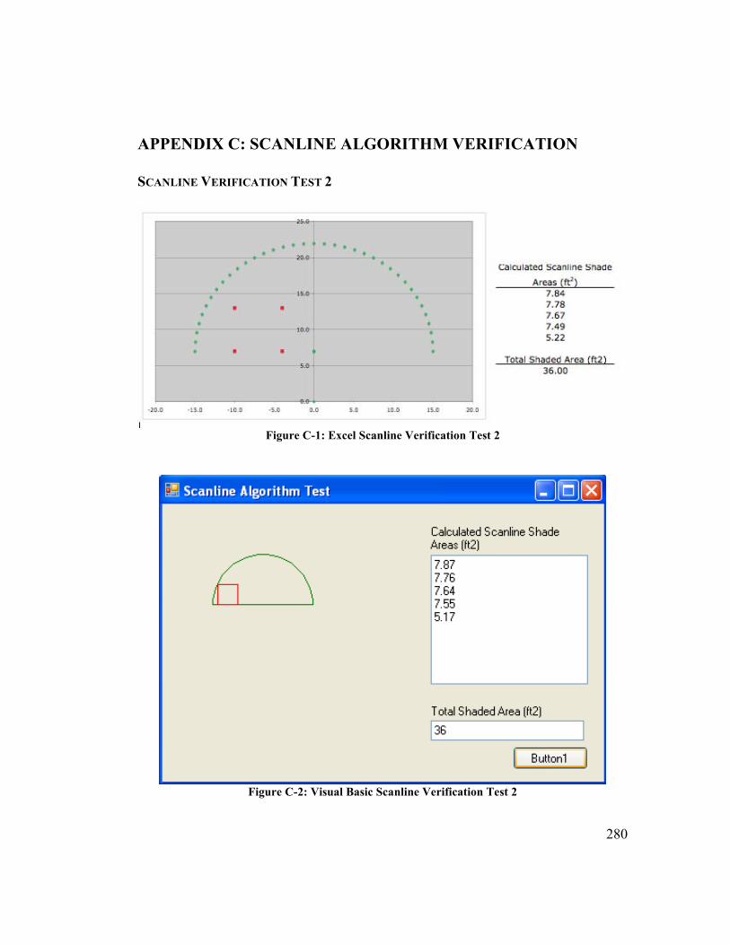
280
APPENDIX C: SCANLINE ALGORITHM VERIFICATION
SCANLINE VERIFICATION TEST 2
Figure C-1: Excel Scanline Verification Test 2
Figure C-2: Visual Basic Scanline Verification Test 2
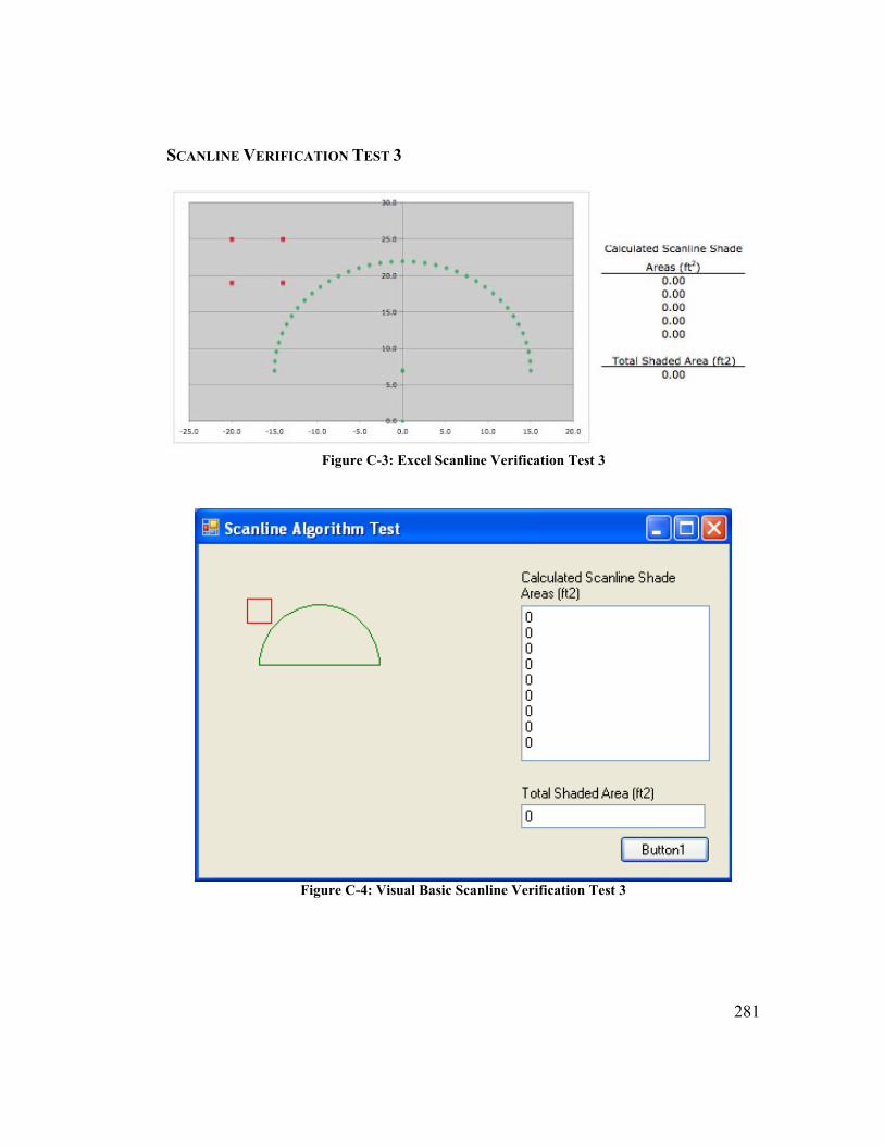
281
SCANLINE VERIFICATION TEST 3
Figure C-3: Excel Scanline Verification Test 3
Figure C-4: Visual Basic Scanline Verification Test 3
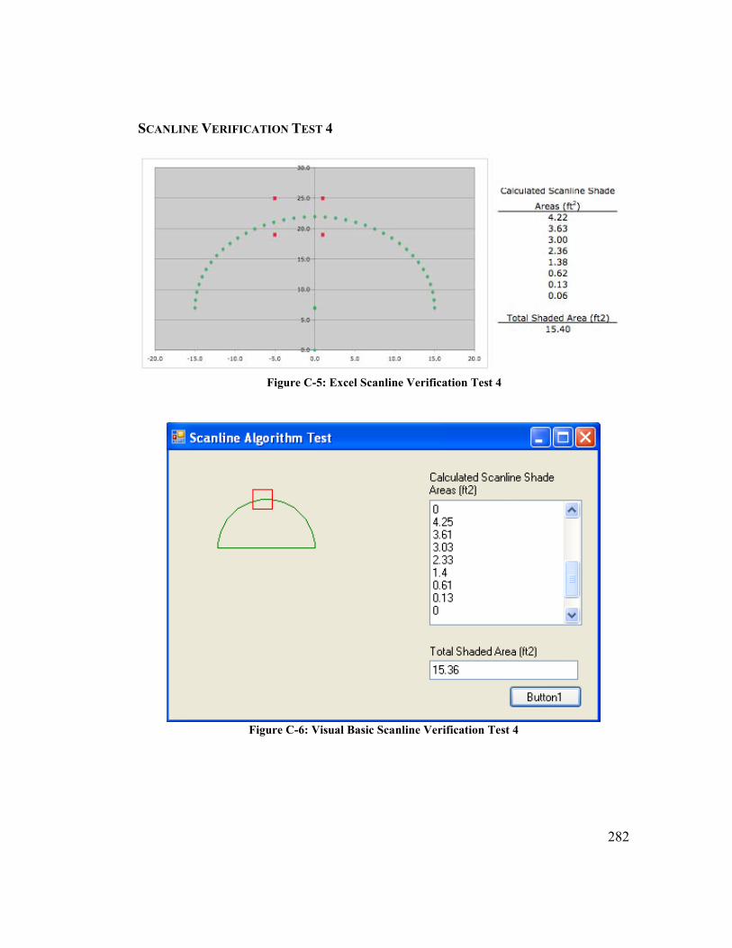
282
SCANLINE VERIFICATION TEST 4
Figure C-5: Excel Scanline Verification Test 4
Figure C-6: Visual Basic Scanline Verification Test 4

283
SCANLINE VERIFICATION TEST 5
Figure C-7: Excel Scanline Verification Test 5
Figure C-8: Visual Basic Scanline Verification Test 5
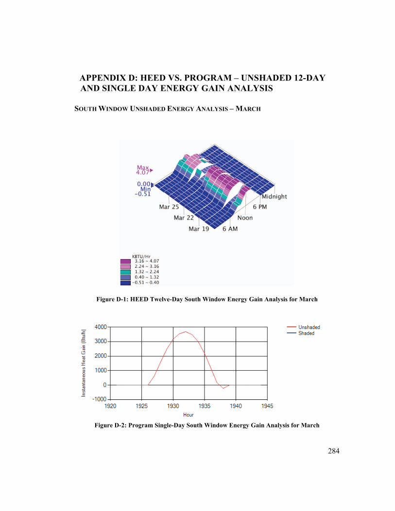
284
APPENDIX D: HEED VS. PROGRAM – UNSHADED 12-DAY
AND SINGLE DAY ENERGY GAIN ANALYSIS
SOUTH WINDOW UNSHADED ENERGY ANALYSIS – MARCH
Figure D-1: HEED Twelve-Day South Window Energy Gain Analysis for March
Figure D-2: Program Single-Day South Window Energy Gain Analysis for March
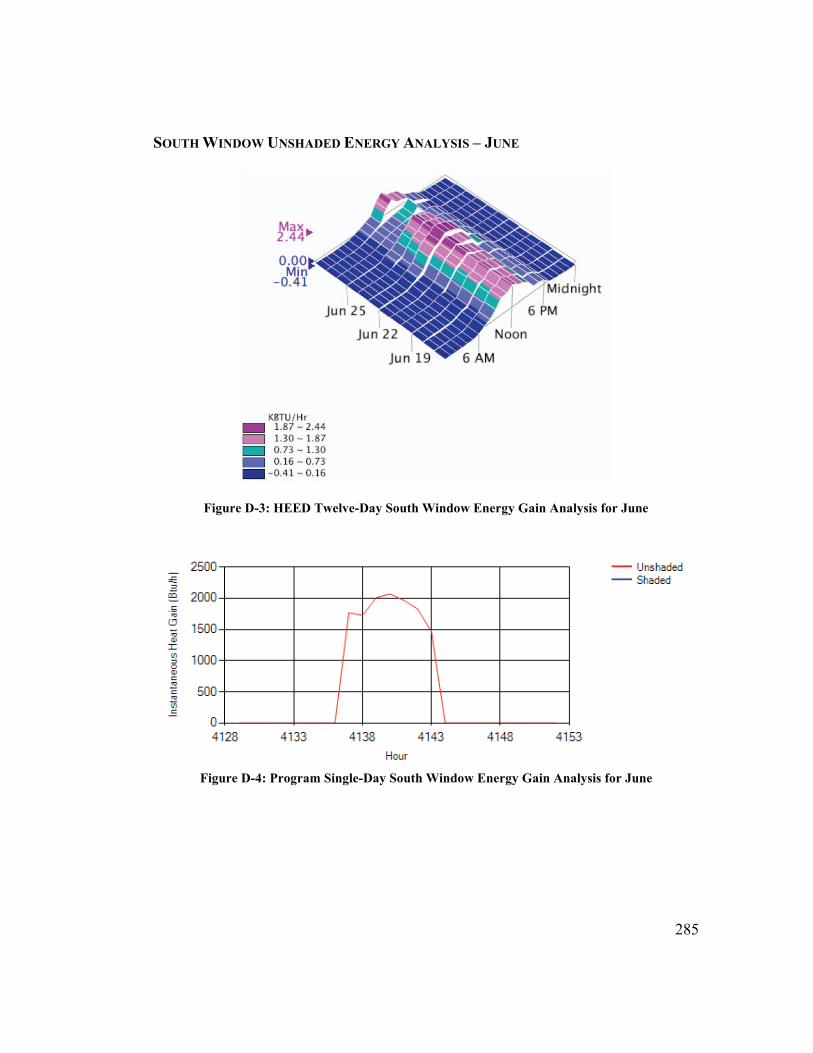
285
SOUTH WINDOW UNSHADED ENERGY ANALYSIS – JUNE
Figure D-3: HEED Twelve-Day South Window Energy Gain Analysis for June
Figure D-4: Program Single-Day South Window Energy Gain Analysis for June
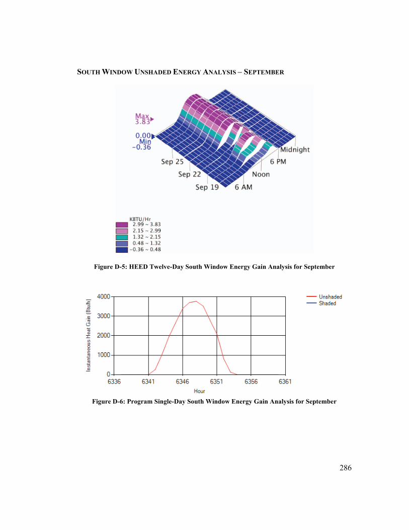
286
SOUTH WINDOW UNSHADED ENERGY ANALYSIS – SEPTEMBER
Figure D-5: HEED Twelve-Day South Window Energy Gain Analysis for September
Figure D-6: Program Single-Day South Window Energy Gain Analysis for September
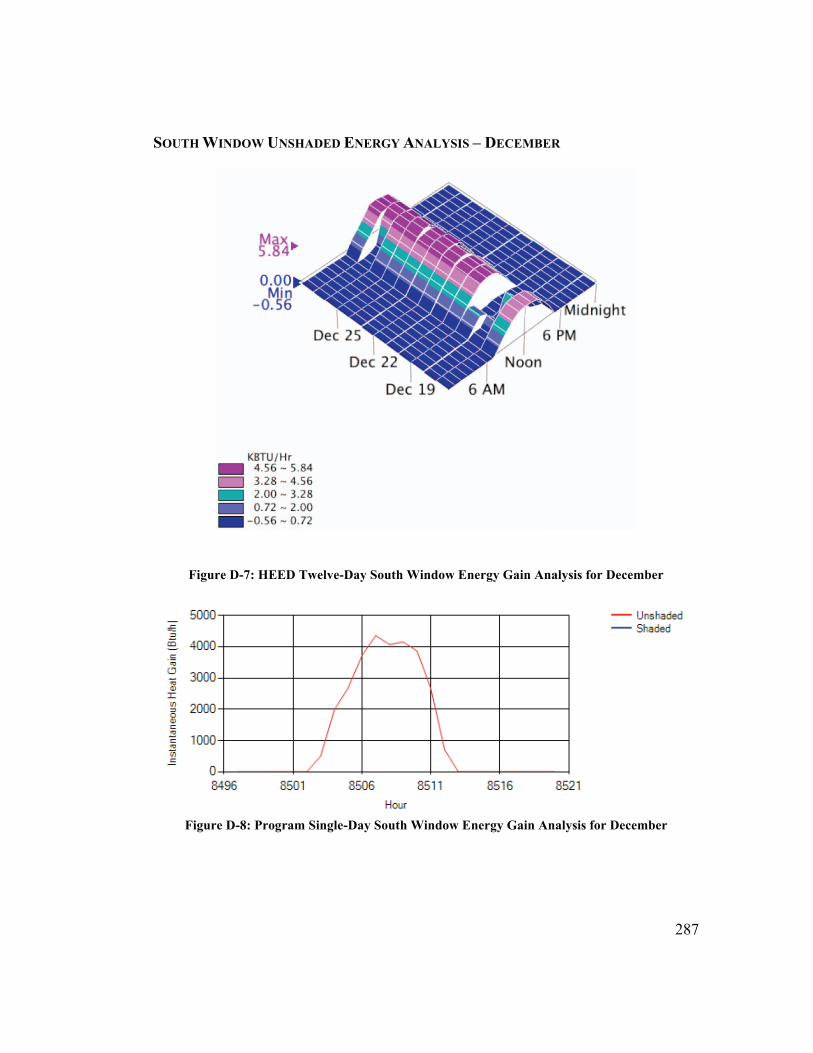
287
SOUTH WINDOW UNSHADED ENERGY ANALYSIS – DECEMBER
Figure D-7: HEED Twelve-Day South Window Energy Gain Analysis for December
Figure D-8: Program Single-Day South Window Energy Gain Analysis for December

288
WEST WINDOW UNSHADED ENERGY ANALYSIS – MARCH
Figure D-9: HEED Twelve-Day West Window Energy Gain Analysis for March
Figure D-10: Program Single-Day West Window Energy Gain Analysis for March
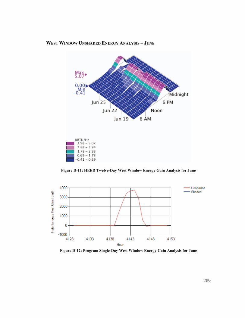
289
WEST WINDOW UNSHADED ENERGY ANALYSIS – JUNE
Figure D-11: HEED Twelve-Day West Window Energy Gain Analysis for June
Figure D-12: Program Single-Day West Window Energy Gain Analysis for June

290
WEST WINDOW UNSHADED ENERGY ANALYSIS – SEPTEMBER
Figure D-13: HEED Twelve-Day West Window Energy Gain Analysis for September
Figure D-14: Program Single-Day West Window Energy Gain Analysis for September
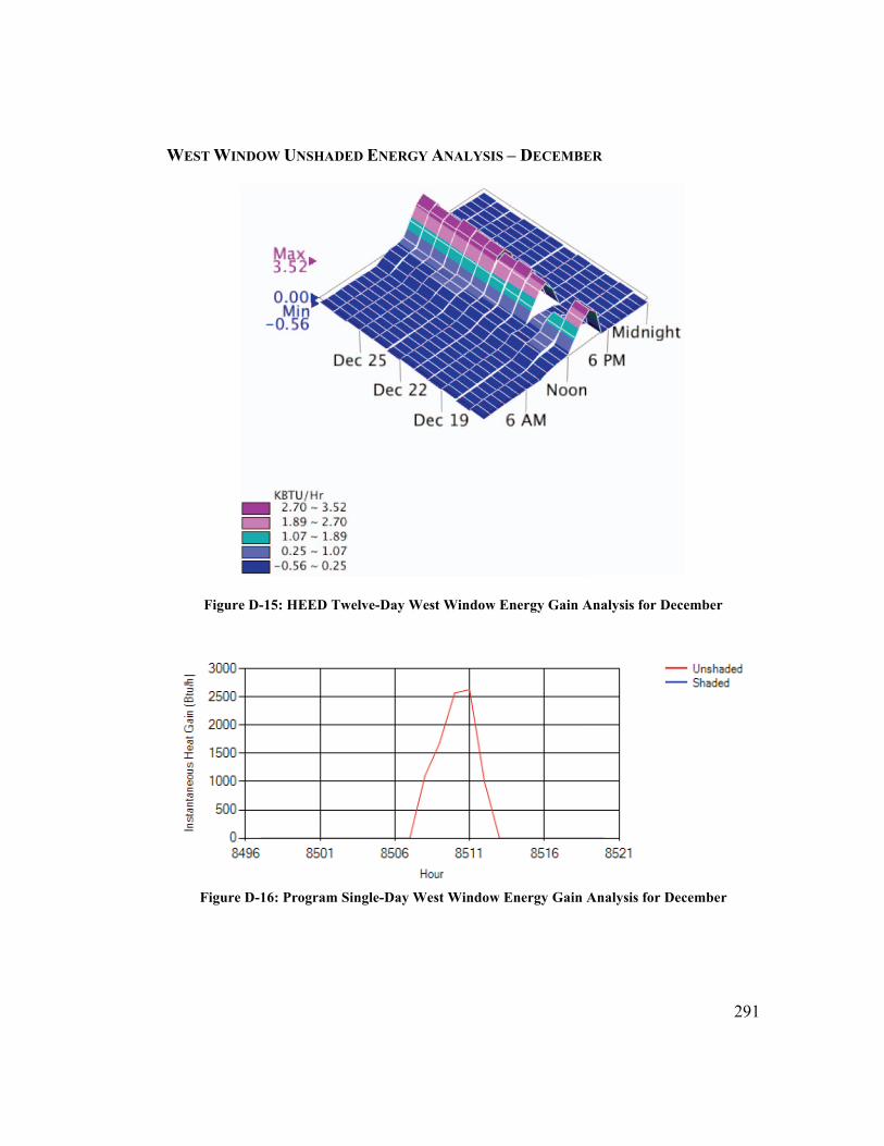
291
WEST WINDOW UNSHADED ENERGY ANALYSIS – DECEMBER
Figure D-15: HEED Twelve-Day West Window Energy Gain Analysis for December
Figure D-16: Program Single-Day West Window Energy Gain Analysis for December

![future visions: athens [2] - İTÜ...> Landscape Urbanism: A Manual for the Machinic Landscape, Mohsen Mostafavi, Ciro Najle, (AA Publications, 2004) > The Rise of the Network Society,](https://img.pdfslide.us/doc/110x75/6079769b1942191e1b21a762/future-visions-athens-2-toe-landscape-urbanism-a-manual-for-the.jpg)