Land–Ocean Warming Contrast over a Wide Range of …pog/src/byrne_land_ocean_warming_contrast_2013.pdf · Surface temperatures increase at a greater rate over land than ocean in

Land–Ocean Warming Contrast over a Wide Range of Climates: ConvectiveQuasi-Equilibrium Theory and Idealized Simulations

MICHAEL P. BYRNE AND PAUL A. O’GORMAN

Massachusetts Institute of Technology, Cambridge, Massachusetts

(Manuscript received 10 May 2012, in final form 28 November 2012)

ABSTRACT

Surface temperatures increase at a greater rate over land than ocean in simulations and observations of

global warming. It has previously been proposed that this land–ocean warming contrast is related to different

changes in lapse rates over land and ocean because of limitedmoisture availability over land. A simple theory

of the land–oceanwarming contrast is developed here inwhich lapse rates are determined by an assumption of

convective quasi-equilibrium. The theory predicts that the difference between land and ocean temperatures

increases monotonically as the climate warms or as the land becomes more arid. However, the ratio of dif-

ferential warming over land and ocean varies nonmonotonically with temperature for constant relative hu-

midities and reaches a maximum at roughly 290 K.

The theory is applied to simulations with an idealized general circulation model in which the continental

configuration and climate are varied systematically. The simulated warming contrast is confined to latitudes

below 508when climate is varied by changes in longwave optical thickness. The warming contrast depends on

land aridity and is larger for zonal land bands than for continents with finite zonal extent. A land–ocean

temperature contrast may be induced at higher latitudes by enforcing an arid land surface, but its magnitude is

relatively small. The warming contrast is generally well described by the theory, although inclusion of a land–

ocean albedo contrast causes the theory to overestimate the land temperatures. Extensions of the theory are

discussed to include the effect of large-scale eddies on the extratropical thermal stratification and to account

for warming contrasts in both surface air and surface skin temperatures.

1. Introduction

A robust feature of simulations and observations of

global warming is that land surface temperatures in-

crease to a greater extent than ocean surface tempera-

tures (e.g., Manabe et al. 1991; Sutton et al. 2007). This

land–ocean surface warming contrast is not predom-

inantly a transient effect due to the different thermal

inertias of the land and ocean regions; rather, it appears

to be a fundamental response of the climate system to

global warming that persists in the equilibrium response

of the system. In addition to the importance of the land–

ocean warming contrast for societal impacts of climate

change, it may also be expected to play a dynamical role

by influencing features of the general circulation such as

stationary waves.

Several previous studies have investigated the land–

ocean warming contrast in fully coupled general circu-

lationmodel (GCM) simulations (e.g., Sutton et al. 2007;

Lambert and Chiang 2007; Fasullo 2010; Boer 2011).

The contrast is often characterized in terms of an am-

plification factor A [ DTL/DTO, where D indicates a

change between two climates and TL and TO are the

surface air temperatures over land and ocean, re-

spectively. Using 20 models from the World Climate

Research Programme’s CoupledModel Intercomparison

Project phase 3 (WCRP CMIP3) (Meehl et al. 2007),

Sutton et al. (2007) found that the amplification factor

based on global-mean surface air temperature varies

from 1.36 to 1.84 depending on the model, with a multi-

model mean of 1.55. The amplification factor also varies

with latitude, with a localminimumof;1.2 in the tropics

and a maximum of ;1.6 in the subtropics in the multi-

model mean. The amplification factor remains approx-

imately constant as the radiative forcing increases, but it

is somewhat smaller in equilibrium simulations with

a ‘‘slab’’ ocean (multimodel mean of 1.33) compared

Corresponding author address: Michael Byrne, Massachusetts

Institute of Technology (54-1815), 77Massachusetts Ave., Cambridge,

MA 02139-4307.

E-mail: [email protected]

4000 JOURNAL OF CL IMATE VOLUME 26

DOI: 10.1175/JCLI-D-12-00262.1

� 2013 American Meteorological Society

with transient simulations with a coupled atmosphere–

ocean model (multimodel mean of 1.55).

Analysis of a variety of coupled and uncoupled GCM

simulations shows that the land–ocean warming contrast

is present in interannual variability and suggests that the

interaction between ocean and land is asymmetric,

causing the land surface temperature to be more sensi-

tive to the ocean surface temperature than the ocean

surface temperature is to the land surface temperature

(Compo and Sardeshmukh 2008; Dommenget 2009)

[although the degree of asymmetry is not generally

agreed upon (Lambert et al. 2011)]. It has been further

argued that the majority of land warming in response to

anthropogenic forcing is actually forced indirectly by the

warming ocean and not by local radiative forcing

(Dommenget 2009).

The land–ocean surface warming contrast is also evi-

dent in the observational record of recent decades

(Sutton et al. 2007; Lambert and Chiang 2007; Drost

et al. 2011). The amplification factors derived from ob-

servations andmodels have similar latitudinal structures

and comparable low-latitude (408S–408N) magnitudes

(Sutton et al. 2007). However, agreement between ob-

servations and models, and indeed between the models

themselves, is poor in the middle to high latitudes of the

Northern Hemisphere, which may be partly related to

the disparate ice and land surface parameterizations and

aerosol forcings employed by the various models.

Differences in the surface energy budget over land

and ocean have been invoked to account for the exis-

tence of an equilibrium warming contrast (e.g., Manabe

et al. 1991; Sutton et al. 2007). Assume, for example, that

a surface radiative forcing is applied with equal magni-

tude over land and ocean. Because of less surface mois-

ture availability over land, cooling by dry-sensible and

longwave-radiative fluxes represents a greater portion

of the increase in surface cooling required to balance

the energy budget, implying a land–ocean contrast in

changes in surface air temperature and air–surface

temperature disequilibrium (the difference between

surface air and surface skin temperature). This simple

argument suggests that the land–ocean warming contrast

should be larger for drier land regions, as is found to some

extent in simulations and observations, although changes

in aridity and low cloud cover are also important, even

in moist regions (Joshi et al. 2008; Doutriaux-Boucher

et al. 2009; Fasullo 2010). Lambert and Chiang (2007)

extend the energy approach by including a land–ocean

heat flux, which helps to maintain the relatively constant

amplification factor that is a feature of observations and

simulations (Huntingford and Cox 2000; Sutton et al.

2007). Although these arguments provide an intuitive

understanding of why one might expect a land–ocean

warming contrast to exist, the surface energy budget alone

is not sufficient to give a quantitative estimate of the

warming contrast: even if changes in surface relative hu-

midity, soil moisture, and downwelling radiative fluxes are

taken as given, the surface energy budget still depends on

changes in air–surface temperature disequilibrium in ad-

dition to the changes in surface temperature that we wish

to estimate.

Rather than attempting to relate land–ocean temper-

ature differences to local energy budgets, Joshi et al.

(2008) argue that atmospheric processes provide a strong

constraint on the land–ocean warming contrast. Tropo-

spheric lapse rates behave differently over land and

ocean because of limited moisture availability over land.

If a level exists in the atmosphere at which there is no

warming contrast (or no temperature contrast in our

version of the theory), then different changes in lapse

rates over land and ocean imply different changes in

surface air temperature. Furthermore, the constraint

from atmospheric processes may apply over a range of

time scales, and local radiative forcing over land is not

required to obtain an amplification factor greater than

unity. This approach is attractive in that it does not in-

volve surface energy fluxes explicitly (which depend on

several factors in addition to surface temperature), but it

does require an understanding of tropospheric lapse

rates in different regimes.

Our study differs from previous studies by inves-

tigating the land–ocean warming contrast over a wide

range of climates and by comparing theory with simu-

lations from an idealized GCM using a variety of land

configurations. The land configurations chosen provide

control, ocean-only hemispheres that facilitate a straight-

forward comparison of land and ocean temperatures

(with the exception of simulations with a meridional

land band, in which induced stationary waves make in-

terpretations more difficult). Our idealized simulations

permit a systematic evaluation of the response of land–

ocean temperature contrasts to radiative forcing; such

a systematic evaluation is more difficult to accomplish

with a full-complexity GCM in which ocean circulations,

topography, ice and snow coverage, fixed continents, and

other factors make interpretations more troublesome.

We begin by developing a simple theory to estimate

the magnitude of the warming contrast (section 2). The

theory is based on the hypothesis of Joshi et al. (2008)

that the contrast arises from different lapse rates over

land and ocean, owing to differences in moisture avail-

ability, although we make somewhat different assump-

tions from Joshi et al. (2008) regarding how the lapse

rates are set. We then explore how the warming contrast

varies with latitude and with land configuration in a

range of simulations with the idealizedGCM (section 3).

15 JUNE 2013 BYRNE AND O ’GORMAN 4001

Climate is varied in the idealized GCM by prescribing

changes in longwave absorber as a representation of

changes in greenhouse gas concentrations or by pre-

scribing different evaporative fractions to directly test the

effects of land aridity. Results from the simulations are

presented for subtropical (section 4) and higher-latitude

(section 5) land surfaces. Extensions of the theory to

account for the effect of eddies on the extratropical

stratification are discussed (section 5b). The sensitivities

of the land–ocean warming contrast to water vapor ra-

diative feedbacks and land–ocean albedo contrasts are

assessed with additional sets of simulations (section 6).

In all cases, the simulation results are compared to the

simple theory. Differences between warming contrasts

as measured by surface air temperatures and surface

skin temperatures are also described (section 7). The

paper concludes with a summary and a brief discussion

of outstanding questions (section 8).

2. Theory

We introduce a simple theory that allows for the es-

timation of the land–ocean surface air temperature dif-

ference and warming contrast based on the ocean

surface air temperature TO and the surface relative hu-

midities over ocean and land, HO and HL, respectively.

We aremotivated by the hypothesis of Joshi et al. (2008)

that the land–ocean contrast is constrained by different

changes in lapse rates over land and ocean caused by

differences in surface moisture availability.

Joshi et al. (2008) make the assumption that the land–

ocean warming contrast vanishes sufficiently high in the

atmosphere. We make the stronger assumption that the

land and ocean temperatures (rather than their changes)

are equal sufficiently high in the atmosphere. This as-

sumption simplifies the analysis and should be approx-

imately valid in the tropics because of weak temperature

gradients in the tropical free troposphere (e.g., Sobel

and Bretherton 2000). Idealized GCM simulations dis-

cussed later suggest that the assumption of equal land

and ocean temperatures aloft may also be adequate in

some cases in the extratropics.

Our second assumption is that lapse rates are moist

adiabatic in the mean over land and ocean. By moist

adiabatic lapse rates, we mean dry adiabatic lapse rates

below the lifted condensation level (LCL) and satu-

rated moist adiabatic lapse rates above it, such that

a parcel lifted from near the surface is neutrally buoyant

with respect to the mean state of the atmosphere.1 This

assumption implies that our theory is appropriate to the

tropics and falls into the class of theories based on con-

vective quasi-equilibrium (e.g., Arakawa and Schubert

1974; Emanuel 2007). In our application of convective

quasi-equilibrium, convection is assumed to be sufficiently

active so as to maintain moist adiabatic lapse rates in the

mean despite large-scale dynamical and radiative forcing.

With these two assumptions, the lapse rates over land

and ocean only differ in the vertical range between the

LCLover ocean and the LCLover land (Fig. 1). The LCL

is higher over land because of lower surface moisture

availability. In the vertical range between the LCLs,

a saturated moist adiabatic lapse rate Gm* occurs over

ocean and a dry adiabat Gd occurs over land. Warming

results in a reduction in Gm* but leaves Gd unchanged.

Combined with the assumption of equal temperatures

above the LCLs, this implies a greater surface warming

over land than ocean. Changes in surface relative hu-

midity affect the LCLs and may also modify the warm-

ing contrast. Note that the higher LCL over land implies

not only a land–ocean warming contrast, but also a

higher surface temperature over land than ocean in the

current climate, all else being equal.

Our assumptions allow for the prediction of the land

surface air temperature from the ocean surface air

temperature and the surface relative humidities over

land and ocean. For example, using the air temperature

and relative humidity at the ocean surface, we can in-

tegrate upward along themoist adiabatic lapse rate from

the surface to the level at which the temperature

FIG. 1. Schematic diagram of potential temperature vs height for

moist adiabats over land and ocean and equal temperatures at

upper levels. A land–ocean surface air temperature contrast is

implied by different LCLs over land and ocean.

1 Joshi et al. (2008) do not assume that mean lapse rates are

moist adiabatic over land and ocean in this sense, but instead give

an illustrative example in which the lower-tropospheric lapse rate

is a weighted average of dry and saturated moist adiabatic lapse

rates, with weightings depending on relative humidity.


becomes equal over land and ocean. Using this tem-

perature aloft and the surface relative humidity over

land, we can then solve iteratively for the surface air

temperature over land (again assuming moist adiabatic

lapse rates). In practice, it is simpler to use the equiva-

lent potential temperature ue, which we take to be con-

served for dry and pseudoadiabatic displacements. The

theory amounts to assuming equal surface air ue over land

and ocean:

ue(TL,HL)5 ue(TO,HO) . (1)

Figure 2a shows temperature contrasts for solutions to

Eq. (1) for a fixed ocean surface relative humidity of 80%

and a range of values of ocean surface air temperature

and land surface relative humidity.2 The temperature

contrast is an increasing function of temperature and

a decreasing function of surface relative humidity over

land; it reaches a value of 25 K for an ocean temperature

of 320 K and a land surface relative humidity of 20%.

In the limit of an infinitesimal change in climate, the

amplification factor may be written as

A5dTL

dTO

5›TL

›TO

1›TL

›HL

dHL

dTO

1›TL

›HO

dHO

dTO

5AT 1AHL 1AH

O , (2)

where AT 5 ›TL/›TO is the component of the ampli-

fication factor arising from changes in temperature

alone, while AHL 5 (›TL/›HL)(dHL/dTO) and AH

O 5(›TL/›HO)(dHO/dTO) are the contributions toA due to

changes in land and ocean surface relative humidities,

respectively. All partial derivatives are calculated as-

suming equal equivalent potential temperatures over

land and ocean according to (1). The amplification factor

at constant relative humidity,AT, increases monotonically

with decreasing relative humidity over land (Fig. 2b).

However, the amplification factor varies nonmonotoni-

cally with temperature and has a maximum at an ocean

surface air temperature of roughly 290 K for the relative

humidities considered here. This nonmonotonic behav-

ior arises because, although the saturated moist adia-

batic lapse rate is amonotonically decreasing function of

temperature, it has an inflection point with respect to

temperature at approximately 273 K (calculated at

900 hPa), which gives rise to the peak in the amplifica-

tion factor. The amplification factor depends on the

lapse rates in the layer between the LCLs over land and

ocean (cf. Fig. 1), and the temperature of this layer is

lower than that of the surface. As a result, the maximum

in Fig. 2b occurs at a surface air temperature that is

higher than the inflection-point temperature of 273 K.

Changes in surface relative humidity under global

warming must also be taken into account; decreases of up

to 2%K21 over landwere foundbyO’Gorman andMuller

(2010) for a multimodel mean of CMIP3 simulations.

FIG. 2. Theoretical values of (a) the land–ocean surface air

temperature differenceTL2 TO (contour interval 5 K) and (b) the

amplification factor AT 5 ›TL/›TO (contour interval 0.1) at con-

stant relative humidities for a range of surface relative humidities

over land and temperatures over ocean. Surface relative humidity

over ocean is fixed at 80%. The temperature differences and am-

plification factors are calculated by numerically solving the equal

equivalent potential temperature Eq. (1).

2 We calculate ue using Eq. (9.40) from Holton (2004), with the

temperature at the LCL evaluated using Eq. (22) from Bolton

(1980). It will later be important that the ue used is consistent with

the convection scheme in the idealized GCM. We tested this by

calculating the land–ocean surface air temperature contrast TL 2TO implied by (1) using two different means of calculating ue: first,

using the ue formula mentioned above, and second, by lifting

a surface air parcel pseudoadiabatically to the top pressure level of

theGCM (at which essentially all water has been removed from the

parcel) using the saturated moist adiabatic lapse rate that is in-

corporated in the GCM (Appendix D.2 of Holton 2004) and then

returning to the surface along a dry adiabat. For example, based on

a land surface relative humidity of 40%, an ocean surface relative

humidity of 80%, and an ocean surface air temperature of 290 K,

the land–ocean temperature contrast was approximately 6 K and

the difference between the two estimates described above was

0.25 K. Thus, we conclude that the formula used for ue is adequate

for our study.


The change in land surface air temperature for a given

change in land surface relative humidity at constant ocean

surface air temperature (›TL/›HL) is plotted in Fig. 3a.

For an ocean surface air temperature of 295 K and land

and ocean surface relative humidities of 50% and 80%,

respectively, ›TL/›HL ’ 20.2 K %21, and taking dHL/

dTO ’ 22% K21, we find that AHL ’ 0:4. This demon-

strates that changes in land relative humidity may con-

tribute significantly to the amplification factor according

to the theory.

Changes in ocean surface relative humidity in simula-

tions of climate change are generally smaller than changes

over land (O’Gorman and Muller 2010) and are thought

to be energetically constrained (Schneider et al. 2010).

For a typical increase in ocean surface relative humidity of

0.5% K21, and again taking an ocean surface air temper-

ature of 295 K and land and ocean surface relative hu-

midities of 50% and 80%, respectively, we find that ›TL/

›HO ’ 0.15 K %21 (Fig. 3b) and AHO ’ 0:08, which is

considerably smaller than the contribution from land rel-

ative humidity variations (calculated above as AHL ’ 0:4).

Given that the theory relies on lapse rates being close

tomoist adiabatic in themean, as follows from convective

quasi-equilibrium in the convecting regions of the tropics,

we refer to it as a convective quasi-equilibrium theory of

the surface warming contrast. In the presence of other

stabilizing influences on the stratification in addition

to convection (such as large-scale eddies in the extra-

tropics) the theory is not strictly applicable, although it

may still be a useful guide. The extension of the theory

to include the effects of large-scale eddies on the extra-

tropical thermal stratification is discussed in section 5b.

A simple generalization of the theory is possible,

also consistent with the concept of convective quasi-

equilibrium, in which lapse rates are not assumed to be

exactly moist adiabatic, but rather, the departures of

lapse rates from moist adiabatic are assumed to remain

constant as climate changes. This generalized theory may

be formulated by assuming that the surface air equivalent

potential temperatures are not necessarily equal over land

and ocean, but that their changes are. The land–ocean

warming contrast will be higher than for the standard

theory if the surface air equivalent potential temperature

is higher over ocean than land. The generalized theory

does not give more accurate predictions for the idealized

simulations presented here, but it may be useful for more

realistic simulations or observations.

3. Idealized GCM

a. Land configurations

The idealized GCM has a lower boundary consisting

of various configurations of land and a mixed-layer

ocean (Fig. 4). Simulations are performed with zonal

land bands in the subtropics (208–408N) and extratropics

(458–658N), a continent of finite zonal extent (208–408N,

08–1208E), and a meridional land band (08–608E).

b. Model and simulations

We use a moist idealized GCM similar to that of

Frierson et al. (2006) and Frierson (2007), with the spe-

cific details documented by O’Gorman and Schneider

(2008b), except for the introduction of land hydrology

(described later in this section) and an alternative radi-

ation scheme that allows for water vapor radiative

feedback (described in section 6a). The model is based

on a version of the Geophysical Fluid Dynamics Labo-

ratory (GFDL) dynamical core and solves the hydrostatic

primitive equations spectrally at T42 resolution with 30

vertical sigma levels. Moist convection is parameterized

using a simplified version of the Betts–Miller scheme

(Frierson 2007), in which temperatures are relaxed to

amoist adiabat and humidities are relaxed to a reference

FIG. 3. Theoretical values for the partial derivatives of land

surface air temperature with respect to (a) surface relative hu-

midity over land (›TL/›HL) and (b) surface relative humidity over

ocean (›TL/›HO) as a function of land relative humidity and ocean

temperature [contour interval 0.2 K %21 in (a) and 0.1 K %21 in

(b)]. Surface relative humidity over ocean is fixed at 80%. The

partial derivatives are calculated by numerically solving the equal

equivalent potential temperature Eq. (1).


profile with a relative humidity of 70%. A large-scale

condensation scheme prevents gridbox supersaturation.

Reevaporation of precipitation is not permitted, and only

the vapor–liquid phase change of water is considered. The

top-of-atmosphere insolation is a representation of an

annual-mean profile, and there is no diurnal cycle.

Longwave radiative fluxes are calculated using a two-

stream gray radiation scheme, and shortwave heating is

specified as a function of pressure and latitude. A range

of climates is simulated by varying the longwave optical

thickness as a representation of the radiative effects of

changes in water vapor and other greenhouse gases. In

the default radiation scheme, the longwave optical

thickness is specified and does not depend explicitly on

the water vapor field, excluding all radiative feedbacks

of water vapor or clouds. Both longwave and shortwave

cloud radiative effects are excluded in the model. The

longwave optical thickness is specified by t 5 atref,

where tref is a function of latitude and pressure, and the

parameter a is varied3 over the range 0.2 # a # 6. The

reference value of a 5 1 corresponds to an Earth-like

climate with a global-mean surface air temperature of

288 K for the simulation with a subtropical land band.

Land and ocean surfaces have the same albedo

(0.38) and heat capacity (corresponding to a layer of

liquid water of depth 1 m and specific heat capacity

3989 J kg21 K21). The effect of a land–ocean albedo

contrast on thewarming contrast is explored in section 6b.

Horizontal heat transport is not permitted below ei-

ther surface. Surface fluxes are calculated using bulk

aerodynamic formulae and Monin–Obukhov similar-

ity theory, with roughness lengths of 5 3 1023 m for

momentum and 1025 m for moisture and sensible heat

over both land and ocean. A k-profile scheme is used to

parameterize boundary layer turbulence (Troen and

Mahrt 1986).

The simple bucket model of Manabe (1969) is used to

simulate the land surface hydrology. The field capacity

SFC in the bucket model is the maximum amount of

water that can be held per unit area of land surface and

has dimensions of depth. Field capacity generally de-

pends on soil type, vegetation, and other factors, but we

set SFC5 0.15 m for simplicity (as inManabe 1969). Soil

moisture S also has dimensions of depth and evolves

according to

dS

dt5

�P2E if S, SFC or P#E

0 if S5 SFC and P.E ,

where P and E are the precipitation and evaporation

rates, respectively. Accordingly, soil moisture accu-

mulates when precipitation exceeds evaporation until

the field capacity is reached, at which point any sub-

sequent excess of precipitation over evaporation is

assumed to run off. Evaporation over land is given by

EL 5 bE0, where b is the evaporative fraction and E0 is

the potential evaporation rate (the evaporation rate

obtained over a saturated land surface using bulk

aerodynamic formulae). The evaporative fraction b is

specified as a linear function of soil moisture up to an

upper bound of 1:

b5

�1 if S$ gSFCS/(gSFC) if S, gSFC ,

where g 5 0.75. This definition ensures that the soil

moisture cannot become negative and that the potential

evaporation rate is reached before soil moisture rea-

ches the field capacity. Although the bucket model ig-

nores complexities such as canopy cover and stomatal

effects [see Seneviratne et al. (2010) for a review of soil

moisture–climate interactions], it is adequate for the

purposes of exploring the effect of limited surface mois-

ture availability on the response of surface air tempera-

tures and atmospheric lapse rates to changes in radiative

forcing.

Simulations are generally spun up from an isothermal

rest state over 3000 days for a, 1 and 1000 days for a$

1, with the exception of the simulations with amidlatitude

zonal land band and prescribed evaporative fractions

(1500 days) and the simulations with a meridional land

band (3000 days). Longer spin-up times are required in

colder climates because specific humidities andwater vapor

fluxes are smaller in magnitude, with the result that soil

moisture values take longer to reach statistical equilibrium.

FIG. 4. Simulations are performed using a variety of land con-

figurations: zonal bands (a) from 208 to 408N and (b) from 458 to658N, (c) continent spanning 208–408N and 08–1208E, and

(d) meridional band from 08 to 608E.

3 There are nine simulations for each of the subtropical and

midlatitude zonal land bands and the subtropical continent (a values

of 0.2, 0.4, 0.7, 1.0, 1.5, 2.0, 3.0, 4.0, and 6.0).


Time averages are taken over the 500-day period after

spinup (or over the 1000 days after spinup in the case of the

simulations with a midlatitude zonal band and prescribed

evaporative fraction and those with a meridional land

band). Similar results are generally found using a 200-day

average. For example, differences between the land–ocean

temperature contrast for the 200- and 500-day averages are

less than 0.3 K for the subtropical land band simulations.

c. Zonal-mean climatology (subtropical zonal landband)

Figure 5 shows the mean potential temperature, merid-

ional streamfunction, and relative humidity for three sim-

ulations (a 5 0.4, 1, and 6) with a subtropical zonal land

band from208 to 408N. In the cold simulation (a5 0.4), the

land does not have a strong influence on the atmospheric

state beyond a moderate decrease in the low-level relative

humidity over the land band. The reduction in relative

humidity is greater in the reference simulation (a5 1), and

it is a dominant feature in the warm simulation (a 5 6), in

which it extends upward from the surface to s’ 0.5, where

s is pressure normalizedby surface pressure. The enhanced

warming over land affects the near-surface temperature

structure by weakening the meridional temperature gra-

dient equatorward of the land band and strengthening the

gradient on the poleward side in the reference simulation;

it causes a reversed temperature gradient on the equator-

ward side of the land band in the warmest simulation.

Shallow monsoon circulations are evident in both the

reference and warmest simulations. The quasi-equilibrium

theory of monsoons associates the upward branch of direct

thermal circulations with local boundary layer maxima in

either equivalent potential temperature or potential tem-

perature (Emanuel 1995). An observational analysis of the

various regional monsoons on Earth by Nie et al. (2010)

shows that two distinct circulation types exist: one is a

deep and moist circulation (with upward branch near the

boundary layer maximum of equivalent potential tem-

perature), and the other is a mixed circulation composed

of a shallow dry cell (with upward branch near the

boundary layer maximum in potential temperature) su-

perimposed on the deep moist cell. The monsoon circu-

lations in our simulations show some similarities to the

FIG. 5. (left) The zonal- and time-mean potential temperature (contour interval 15 K), (middle) Eulerian-mean streamfunction

(contour interval 203 109 kg s21, with negative values given by dashed contours), and (right) relative humidity (contour interval 10%) for

a zonal land band from 208 to 408N in (a) a cold simulation (a5 0.4), (b) the reference simulation (a5 1), and (c) the warmest simulation

(a 5 6). The heavy black bars indicate the position of the subtropical zonal land band (208–408N).


mixed circulations observed by Nie et al. (2010); the ad-

dition of a seasonal cycle to our GCM might lead to a

closer resemblance by shifting the boundary layer maxi-

mum in equivalent potential temperature poleward in

summer. A more detailed study of the changing strength

and character of these monsoonal circulations as the cli-

mate is varied is left to future work.

4. Subtropical warming contrast

a. Subtropical zonal land band

We first consider simulations with a subtropical zonal

land band from 208 to 408N. The land surface air

temperature for a given simulation TL is defined as the

temperature of the lowest atmospheric level (s 5 0.989)

averaged in time and over all land grid points (with area

weighting). Tomakemeaningful comparisons of land and

ocean regions, we define the ocean surface air tempera-

ture to be the average of the lowest-level temperatures

over the corresponding region in the other hemisphere.

For example, in the case of the zonal land band from

208 to 408N, the ocean surface air temperature TO is

calculated by averaging over 208–408S.The land–ocean contrast in temperature is close to

zero in the coldest climate and increases in magnitude as

the climate warms, reaching 19 K in the warmest simu-

lation (Fig. 6). The land–ocean amplification factor has

a mean value of 1.4 over all simulations and varies

nonmonotonically with ocean temperature (Fig. 7). The

mean value is of similar magnitude to the Sutton et al.

(2007) low-latitude (408S–408N) estimates of 1.51 and

1.54 for climate-model simulations and observations,

respectively, although close agreement with our simu-

lations is not necessarily expected given the differences

in continental configuration, surface aridity and heat

capacity, and radiative forcing.

The estimate of TL based on theory matches the

simulated land temperatures well over the full range of

simulations, with an overestimation of TL of order 1 K

in each simulation (dashed–dotted line in Fig. 6). For the

theory, the equivalent potential temperatures in Eq. (1)

are evaluated using TO and the surface relative humid-

ities (evaluated at the lowest model level) averaged in

time and over land or the corresponding region over

ocean. The estimates of the amplification factor from

theory are also accurate (dashed line in Fig. 7). There is

a maximum in the simulated amplification factor at TO ’300 K, which is higher than the temperature at which the

theoretical maximum occurs for constant relative hu-

midities (cf. Fig. 2b), but these should not be directly

compared because of changes in the relative humidities

in the simulations. In the coldest simulation (a 5 0.2),

the surface relative humidities over land and ocean are

51% and 74%, respectively. Ocean relative humidity re-

mains approximately constant over the full range of cli-

mates, but land relative humidity decreases with warming

to 24% in the reference simulation (a 5 1) and remains

roughly unchanged over the warmer simulations (not

shown). The impact of changes in relative humidity is il-

lustrated by comparisonwith the theoretical amplification

factors assuming unchanged relative humidities (dashed–

dotted line in Fig. 7). Not accounting for changes in

FIG. 6. Surface air temperature over ocean (solid line with cir-

cles) and land (dashed line with circles) vs ocean surface air tem-

perature for a subtropical zonal land band from 208 to 408N. Filled

circles denote the reference simulation (a 5 1) here and in sub-

sequent figures. The dashed–dotted line is the estimate of surface

air temperature over land from theory.

FIG. 7. The amplification factor vs ocean surface air temperature

in simulations with a subtropical land band from 208 to 408N (solid

line with circles), from theory (dashed line), and from theory ne-

glecting changes in relative humidity (dashed–dotted line). The

amplification factor is calculated based on temperature differences

between pairs of nearest-neighbor simulations and is plotted

against the midpoint ocean temperature for each pair. The ampli-

fication factor from theory is obtained in the same way, but using

the theoretical estimates of the land temperature (dashed–dotted

line in Fig. 6). The amplification factor from theory neglecting

changes in relative humidities [corresponding to AT in (2)] is

evaluated using the surface relative humidities from the colder of

the pair of simulations when estimating the land temperature in the

warmer simulation.


relative humidity results in a substantial underestimation

of the amplification factor for all but the warmest two

simulations (between which the land relative humidity

increases slightly), indicating that the land–ocean surface

warming contrast is tightly coupled to changes in low-

level relative humidity.

We next examine the accuracy of each of the assump-

tions made in the theory. The assumption that there is

a level at which the land–ocean temperature difference

vanishes is found to hold in our simulations (Fig. 8). The

fact that this level rises as the climatewarms is not an issue

since the theory only requires that such a level exists. The

assumption of moist adiabatic lapse rates below this level

is accurate over ocean, but it is not very accurate over land

(Fig. 9), which may be related to moist convection oc-

curring less frequently over the relatively dry land. The

vertical temperature profile over land in the GCM sim-

ulations is generallymore stable thanmoist adiabatic, and

this is consistent with the slight overestimation of the

land–ocean surface air temperature contrast by the theory

(Fig. 6).

The deviation of the mean thermal stratification from

moist adiabatic over land is not as great as might be

inferred from comparison with a moist adiabat based on

mean surface relative humidity (dashed lines in Fig. 9).

Wemake a second comparison that allows for variability in

low-level relative humidity by using estimated probability

density functions (PDFs) of surface relative humidity

when calculating the moist adiabats. The PDF-weighted

moist adiabatic lapse rate Gpdfm (s) at a given level s is

computed as

Gpdfm (s)5

ð100%0

f (H)Gm(T,H,s) dH , (3)

where f(H) is the PDF of surface relative humidity and

Gm(T, H, s) is the lapse rate at s for a moist adiabat

calculated using a surface air temperature of T and

a surface relative humidity ofH. Figure 9 shows that Gpdfm

is a somewhat better approximation to the simulated

lapse rates over land compared with lapse rates based

on moist adiabats calculated using mean surface relative

humidities. We make a corresponding estimate of TL

using the PDFs of surface relative humidity over land

and ocean rather than the mean values. (We calculate

the temperature at the level at which the land–ocean

contrast vanishes by integrating Gpdfm over ocean from

the surface to that level, and we then solve iteratively

for TL using Gpdfm over land.) The resulting estimates

of TL are almost indistinguishable from the estimates

using mean surface relative humidities (not shown).

These results suggest that although variability in surface

relative humidity over land results in variability in the

LCL and effectively smooths the time-mean lapse rates

in the vertical (Fig. 9b), use of mean surface relative

humidities is still adequate when applying the equal

equivalent potential temperature Eq. (1) to estimate

land temperatures.

b. Subtropical continent

The subtropical warming contrast is further inves-

tigated using a continent that extends from 208 to 408Nand 08 to 1208E (Fig. 4c). The ocean temperatures are

averaged over 208–408S and 08–1208E. The land–ocean

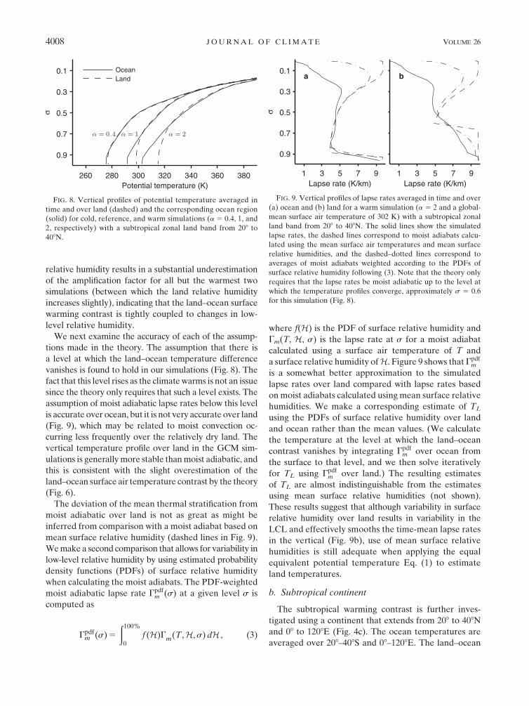
FIG. 8. Vertical profiles of potential temperature averaged in

time and over land (dashed) and the corresponding ocean region

(solid) for cold, reference, and warm simulations (a 5 0.4, 1, and

2, respectively) with a subtropical zonal land band from 208 to408N.

FIG. 9. Vertical profiles of lapse rates averaged in time and over

(a) ocean and (b) land for a warm simulation (a 5 2 and a global-

mean surface air temperature of 302 K) with a subtropical zonal

land band from 208 to 408N. The solid lines show the simulated

lapse rates, the dashed lines correspond to moist adiabats calcu-

lated using the mean surface air temperatures and mean surface

relative humidities, and the dashed–dotted lines correspond to

averages of moist adiabats weighted according to the PDFs of

surface relative humidity following (3). Note that the theory only

requires that the lapse rates be moist adiabatic up to the level at

which the temperature profiles converge, approximately s 5 0.6

for this simulation (Fig. 8).


temperature difference for the continent is smaller than

for the corresponding subtropical land band simulations

in all but the coldest climate (e.g., it is approximately

2 K smaller for a 5 1.5 and an ocean temperature of

297 K). The theoretical estimates match the continental

land–ocean temperature contrasts, although the land

temperatures are slightly overestimated, as for the sub-

tropical band simulations (Fig. 10). The reduced warming

contrast compared to the zonal land band is consistent

with higher surface relative humidity over the continent

(28% over the continent versus 23% over the subtropical

band for a 5 1.5). Higher relative humidity is to be ex-

pected over a continent of finite zonal extent because of

zonal moisture fluxes from surrounding oceanic regions.

c. The effect of aridity

The results above illustrate that limited moisture

availability can generate a land–ocean temperature

contrast and that this contrast increases as the climate

warms in response to radiative forcing. For the simula-

tions discussed so far, the soil moisture and the evapo-

rative fraction have been dynamic quantities that vary in

response to changes in the local balance of evaporation

and precipitation as the climate warms. To isolate the

effect of aridity on the land–ocean temperature contrast,

we perform a series of simulations with fixed longwave

optical thickness (a5 1) and a range of specified values

of the evaporative fraction4 b over a zonal land band

from 208 to 408N. Reducing the evaporative fraction is

a simple means of systematically drying out the land

surface; it may also be taken as an analog for decreased

soil moisture levels in a warmer climate or reduced sto-

matal conductance and evapotranspiration in elevated

CO2 environments (cf. Joshi and Gregory 2008).

For b 5 1, land and ocean are identical in the ideal-

ized GCM. Reducing b from unity inhibits evaporation

from the land surface, and the surface relative humidity

over land decreases. According to our theory (Fig. 2),

a reduction in relative humidity over land, along with

roughly constant relative humidity and temperature

over ocean, implies an increase in temperature over

land so as to maintain equal equivalent potential tem-

peratures over land and ocean. This behavior is found

in our idealized model simulations, with the land–

ocean temperature contrast increasing strongly as b is

lowered, and doing so roughly in accordance with the

theory (Fig. 11a). However, as the land surface relative

humidities decrease, the lapse rates depart to a greater

degree from moist adiabats, and surface air equivalent

potential temperatures over land and ocean diverge,

leading to less precise land temperature estimates from

the theory. The effect of varying b at midlatitudes is

discussed in the next section.

FIG. 10. Surface air temperature over ocean (solid line with

circles) and land (dashed line with circles) vs ocean surface air

temperature for a land continent spanning 208–408N and 08–1208E.The dashed–dotted line is the estimate of the land temperature

from theory.


circles) and land (dashed line with circles) vs evaporative fraction

b for (a) a subtropical zonal land band from 208 to 408N and

(b) a midlatitude zonal land band from 458 to 658N. The dashed–

dotted lines are the estimates of land temperature from theory. The

longwave absorber parameter a has its reference value of unity in

all simulations.

4 Simulations with b values of 0.1, 0.2, 0.3, 0.5, 0.7, 0.8, and 0.9

are performed for both subtropical (208–408N) and midlatitude

(458–658N) zonal land bands.


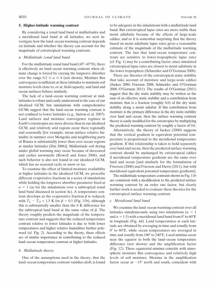
5. Higher-latitude warming contrast

By considering a zonal land band at midlatitudes and

a meridional land band at all latitudes, we next in-

vestigate how the land–ocean warming contrast depends

on latitude and whether the theory can account for the

magnitude of extratropical warming contrasts.

a. Midlatitude zonal land band

For the midlatitude zonal land band (458–658N), there

is effectively no land–ocean warming contrast when cli-

mate change is forced by varying the longwave absorber

over the range 0.2 # a # 6 (not shown). Moisture flux

convergence is sufficient at these latitudes tomaintain soil

moisture levels close to, or at, field capacity, and land and

ocean surfaces behave similarly.

The lack of a land–ocean warming contrast at mid-

latitudes is robust and easily understood in the case of our

idealized GCM, but simulations with comprehensive

GCMs suggest that the land–ocean warming contrast is

not confined to lower latitudes (e.g., Sutton et al. 2007).

Land surfaces and moisture convergence regimes in

Earth’s extratropics aremore diverse than in our idealized

GCM, and relatively arid regions occur there regionally

and seasonally [for example, mean surface relative hu-

midity in summer over Mongolia and neighboring parts

of Russia is substantially lower than over ocean regions

at similar latitudes (Dai 2006)]. Midlatitude soil drying

under global warming may occur because of decreased

and earlier snowmelts (Rowell and Jones 2006), and

such behavior is also not found in our idealized GCM,

which has no seasonal cycle or snow or ice.

To examine the effect of limited moisture availability

at higher latitudes in the idealized GCM, we prescribe

different evaporative fractions in a series of simulations

while holding the longwave absorber parameter fixed at

a 5 1 (as for the simulations over a subtropical zonal

land band discussed in section 4c). A temperature con-

trast develops as the evaporative fraction b is reduced,

with TL 2 TO ’ 1.5 K for b 5 0.1 (Fig. 11b), although

this is substantially smaller than the 6 K difference for

the subtropical land band at the same value of b. The

theory roughly predicts the magnitude of the tempera-

ture contrast and suggests that the reduced temperature

contrast relative to lower latitudes is due to both lower

temperatures and higher relative humidities further pole-

ward (cf. Fig. 2). According to the theory, these effects

are of similar importance in contributing to the reduced

land–ocean temperature contrast at higher latitudes.

b. Midlatitude theory

One of the assumptions used in the theory, that the

land–ocean temperature contrast vanishes aloft, is found

to be adequate in the simulations with amidlatitude land

band. But extratropical lapse rates are more stable than

moist adiabatic because of the effects of large-scale

eddies, and so it is somewhat surprising that the theory

based on moist adiabatic lapse rates gives a reasonable

estimate of the magnitude of the midlatitude warming

contrast. The fact that land–ocean temperature con-

trasts are sensitive to lower-tropospheric lapse rates

(cf. Fig. 1) may be a contributing factor, since simulated

extratropical lapse rates are closest to moist adiabatic in

the lower troposphere (Schneider and O’Gorman 2008).

There are theories of the extratropical static stability

that take account of moisture and large-scale eddies

(Juckes 2000; Frierson 2008; Schneider and O’Gorman

2008; O’Gorman 2011). The results of O’Gorman (2011)

suggest that the dry static stability may be written as the

sum of an effective static stability and a contribution from

moisture that is a fraction (roughly 0.6) of the dry static

stability along a moist adiabat. If this contribution from

moisture is the primary difference in the dry static stability

over land and ocean, then the surface warming contrast

theory is easilymodified for the extratropics bymultiplying

the predicted warming contrast by roughly a factor of 0.6.

Alternatively, the theory of Juckes (2000) suggests

that the vertical gradient in equivalent potential tem-

perature is proportional to the meridional temperature

gradient. If this relationship is taken to hold separately

over land and ocean, then the predicted surface warming

contrast should be unchanged by extratropical eddies

if meridional temperature gradients are the same over

land and ocean [and similarly for the formulation of

Frierson (2008) and Frierson and Davis (2011), but with

meridional equivalent potential temperature gradients].

Themidlatitude temperature contrasts shown in Fig. 11b

are consistent with a modification to the predicted surface

warming contrast by an order one factor, but clearly

further work is needed to evaluate these theories for the

extratropical surface warming contrast.

c. Meridional land band

We examine the land–ocean warming contrast over all

latitudes simultaneously using two simulations (a 5 1

and a5 1.5) with ameridional land band from 08 to 608Ein longitude (Fig. 4d). Land temperatures at each lati-

tude are obtained by averaging in time and zonally from

08 to 608E, while ocean temperatures are averaged in

time and zonally from 1808 to 2408E. Local minima occur

near the equator in both the land–ocean temperature

difference (not shown) and the amplification factor

(Fig. 12). These equatorial minima coincide with atmo-

spheric moisture flux convergence and relatively high

levels of soil moisture. Maxima in the amplification

factor occur at ;158 north and south, coincident with


the descending branches of the Hadley cells. The land–

ocean warming contrast decreases sharply in mid-

latitudes; according to the theory, this reflects both the

poleward increase in relative humidity over land and

the poleward decrease in temperature (Fig. 5). The land

and ocean temperatures are almost equal poleward of

508 latitude. By comparison, mean precipitation exceeds

mean evaporation over ocean poleward of approximately

388 latitude.The theoretical amplification factors are less accurate

for the meridional band simulations than for the sub-

tropical zonal land band or continent, particularly at

subtropical latitudes (Fig. 12). The inaccuracy in this

case is partly due to deviations from moist adiabatic

lapse rates over land, but it may also relate to stationary

waves excited by the land band and the lack of an

ocean-only Southern Hemisphere to compare with. The

amplification factor calculated from theory at constant

surface relative humidities seems to be reasonably ac-

curate at all latitudes (Fig. 12), but this results from

a compensation of errors. The results from the meridi-

onal land band simulations suggest that further work

is needed to better quantify the factors affecting the

accuracy of the theory and to determine how best to

compare land and ocean temperatures in the same

hemisphere.

d. Polar amplification

Given the abundance of land at northern high lati-

tudes, it is difficult to cleanly distinguish in observations

or comprehensive climate model simulations between

polar amplification of temperature changes and land–

ocean warming contrast. A number of processes contrib-

ute to polar amplification, including ice–albedo feedback,

changes in ocean circulation, polar cloud cover, and at-

mospheric heat transport (Holland and Bitz 2003; Hall

2004; Bony et al. 2006). Although the idealized GCM

does not include many of these processes, it still shows a

polar amplification effect under climate change (O’Gorman

and Schneider 2008a; see also Alexeev et al. 2005). The

meridional land band simulations presented here show

negligible land–ocean warming contrast beyond 508latitude (Fig. 12), which implies that the processes in-

volved in establishing a land–ocean temperature con-

trast at low to midlatitudes are distinct from those

responsible for polar amplification in this GCM. We do

note, however, that other work suggests radiative feed-

backs associated with changing water vapor concentra-

tions may be an important component of both polar

amplification and of land–ocean contrasts (Dommenget

and Fl€oter 2011), and land–ocean radiative contrasts are

discussed in the next section.

6. Land–ocean radiative contrasts

The simulations so far have included only a land–

ocean contrast in surface hydrology. Albedo contrasts or

radiative feedbacks from the contrast in humidity could

also affect the land–ocean warming contrast, potentially

in a manner that is not captured by the theory presented

earlier. For instance, decreases in the longwave optical

thickness in response to lower evaporative fraction

could tend to lower the surface temperature over land

(e.g., Molnar and Emanuel 1999) and reduce the land–

ocean temperature contrast.

a. Water vapor radiative feedbacks

To assess the effect of longwave radiative feedbacks

on the land–ocean temperature contrast, an alternative

radiation scheme is used in which the longwave optical

thickness depends on humidity according to

dt

ds5 am1bq , (4)

where t is the longwave optical thickness (set to zero at

the top of the atmosphere), a 5 0.8678 and b 5 1997.9

are nondimensional constants, and q is the specific

humidity [this formulation is similar to that of Merlis

and Schneider (2010), except that the longwave optical

thickness in their study depends on column water vapor

rather than specific humidity]. To facilitate comparison

between simulations with the different radiation schemes,

the values of a and b were chosen by fitting (4) with m51 to the longwave optical thickness averaged from 208to 408N for a reference (a 5 1) aquaplanet simulation

with the default radiation scheme. With this choice of

FIG. 12. The amplification factor vs latitude for warming between

two simulations (a 5 1 and a 5 1.5) with a meridional land band

from 08 to 608E (solid line). The dashed line is the estimate of the

amplification factor from theory, and the dashed–dotted line is the

estimate from theory neglecting changes in relative humidity. In-

terhemispheric asymmetry is indicative of sampling error.


parameters, water vapor is the dominant longwave ab-

sorber at all latitudes for the reference value of m 5 1.

Atmospheric shortwave heating is prescribed as in the

default radiation scheme. Feedbacks associated with

shortwave absorption by water vapor are not considered

here andmay also influence the land–ocean temperature

contrast.

For the subtropical zonal land band (208–408N), we

vary the radiative parameter m over the range 0.4# m#

2 as a representation of the longwave-radiative effect of

changes in greenhouse gases other than water vapor.5

We also consider simulations with specified evaporative

fraction b over the range 0.1 # b # 0.9 and with m 5 1.

The results from both sets of simulations are qualitatively

similar to those performed using the default radiation

scheme (not shown). The land–ocean temperature

contrast is slightly higher than for the default radiation

scheme (by approximately 2 K for a5 4 in the dynamic

soil moisture simulations and by approximately 0.5 K at

b 5 0.5 in the prescribed evaporative fraction simula-

tions). For the midlatitude zonal land band (458–658N),

we consider simulations with prescribed evaporative

fractions over the same parameter range as for the

subtropical land band, and the land–ocean temperature

contrasts are found to be roughly the same as in the

simulations with the default radiation scheme. For both

subtropical and midlatitude land simulations, the theo-

retical estimates are of similar or better accuracy when

compared with the estimates for the simulations with the

default radiation scheme.

There are only modest land–ocean temperature dif-

ferences associated with water vapor radiative contrasts

in our simulations. However, the study of Dommenget

and Fl€oter (2011), using a globally resolved energy bal-

ance model, suggests a greater role for water vapor ra-

diative feedbacks in setting the land–ocean warming

contrast. The idealized nature of the gray radiation scheme

used here precludes us from making any definitive con-

clusions on this issue based on our simulations.

b. Albedo contrast

The importance of land–ocean albedo contrast in

determining the land–ocean warming contrast is as-

sessed using a series of simulations in which the ocean

surface albedo is set to a smaller value of 0.20 and the

land surface albedo remains at 0.38 (the albedo is 0.38

over both land and ocean in our other simulations). Note

that cloud albedo effects are not included in the ideal-

ized GCM, and the surface albedo values used are not

intended to be realistic. The simulations are with

a subtropical zonal land band (208–408N) and use the

default radiation scheme in which the longwave ab-

sorber is varied over the range 0.2 # a # 6.

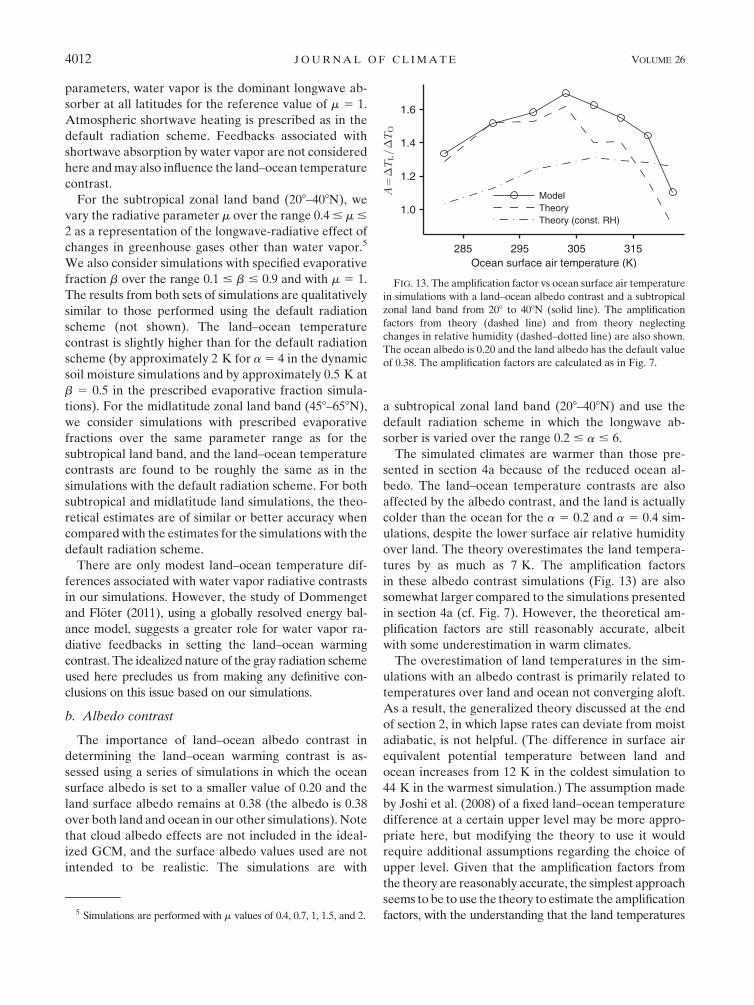
The simulated climates are warmer than those pre-

sented in section 4a because of the reduced ocean al-

bedo. The land–ocean temperature contrasts are also

affected by the albedo contrast, and the land is actually

colder than the ocean for the a 5 0.2 and a 5 0.4 sim-

ulations, despite the lower surface air relative humidity

over land. The theory overestimates the land tempera-

tures by as much as 7 K. The amplification factors

in these albedo contrast simulations (Fig. 13) are also

somewhat larger compared to the simulations presented

in section 4a (cf. Fig. 7). However, the theoretical am-

plification factors are still reasonably accurate, albeit

with some underestimation in warm climates.

The overestimation of land temperatures in the sim-

ulations with an albedo contrast is primarily related to

temperatures over land and ocean not converging aloft.

As a result, the generalized theory discussed at the end

of section 2, in which lapse rates can deviate from moist

adiabatic, is not helpful. (The difference in surface air

equivalent potential temperature between land and

ocean increases from 12 K in the coldest simulation to

44 K in the warmest simulation.) The assumption made

by Joshi et al. (2008) of a fixed land–ocean temperature

difference at a certain upper level may be more appro-

priate here, but modifying the theory to use it would

require additional assumptions regarding the choice of

upper level. Given that the amplification factors from

the theory are reasonably accurate, the simplest approach

seems to be to use the theory to estimate the amplification

factors, with the understanding that the land temperatures

FIG. 13. The amplification factor vs ocean surface air temperature

in simulations with a land–ocean albedo contrast and a subtropical

zonal land band from 208 to 408N (solid line). The amplification

factors from theory (dashed line) and from theory neglecting

changes in relative humidity (dashed–dotted line) are also shown.

The ocean albedo is 0.20 and the land albedo has the default value

of 0.38. The amplification factors are calculated as in Fig. 7.

5 Simulations are performed with m values of 0.4, 0.7, 1, 1.5, and 2.


(as opposed to their changes) may be overestimated

because of albedo contrast.

7. Surface air versus surface skin temperature

The results discussed so far are for surface air temper-

atures, but surface skin temperatures may not respond

in the same way to climate change. Figure 14 shows that

surface skin temperatures are generally larger than sur-

face air temperatures in the subtropical zonal land band

simulations (with the default radiation scheme and al-

bedo values). The amplification factors for the surface

air and surface skin temperatures are similar, but with

somewhat larger amplification factors for surface skin

temperatures below ’305 K, as may be inferred from

Fig. 14. For example, for an ocean surface air temper-

ature of 285 K, the amplification factors based on sur-

face skin and surface air temperatures are 1.67 and

1.48, respectively.

The air–surface temperature disequilibrium (the dif-

ference between the surface air and surface skin tem-

peratures) decreases as the climate warms and does

so more strongly over ocean than over land (Fig. 14).

Changes in the air–surface temperature disequilibrium

may be understood in terms of the surface energy bud-

get, since the surface energy fluxes (particularly the dry

sensible heat flux) are strongly coupled to it. As the

climate warms, evaporative cooling of the surface gen-

erally increases because of the dependence of the satu-

ration vapor pressure on temperature. The increased

evaporative cooling is partially balanced by a reduction

in dry sensible cooling, as reflected in the decrease in air–

surface temperature disequilibrium, in order to maintain

the surface energy balance. Increases in evaporative

cooling are smaller over land than ocean and are in-

hibited by the land becoming increasingly arid, ex-

plaining why the air–surface temperature disequilibrium

does not decrease to the same extent over land, and why

amplification factors are somewhat larger for surface

skin temperatures.

The air–surface temperature disequilibrium may be

large for very arid land regions in a given climate (e.g.,

Pierrehumbert 1995), but this does not mean it will nec-

essarily change greatly in these regions as the climate

changes (as compared to the land–ocean surface warming

contrast). For example, the amplification factors based

on surface air and surface skin temperatures are similar

in our warm simulations in which the land is very arid.

Rather, we may expect these amplification factors to

differ most in regions with substantial changes in aridity

of the land surface as the climate changes.

As discussed in the introduction, it is difficult to build

a theory of the surface warming contrast based solely

on the surface energy budget because changes in both

the surface temperature and air–surface temperature dis-

equilibrium may play an important role in the adjustment

of the surface energy budget over land and ocean. The

theory presented in section 2 based on convective quasi-

equilibrium gives an independent estimate of the land–

ocean warming contrast in surface air temperatures,

whichmay be combinedwith the constraint of the surface

energy budget. As a result, we argue that surface skin

warming contrasts may be best understood based on the

theory for the surface air warming contrasts and an un-

derstanding of changes in the surface energy budget.

Global observational datasets often provide skin tem-

peratures over ocean (sea surface temperatures) and

surface air temperatures over land. For our simulations,

the amplification factors using land surface air tempera-

tures and ocean surface skin temperatures are similar to

those calculated solely from surface skin temperatures

and larger than those calculated solely from surface air

temperatures. Since our theory is most appropriate for

surface air temperatures, it may underestimate amplifi-

cation factors calculated from temperature anomalies in

these mixed observational datasets.

8. Conclusions

Based on the idea that differential changes in lapse

rates over land and ocean constrain the surface warming

contrast (Joshi et al. 2008), we have developed a simple

theory that relates the land surface air temperature and

the land–ocean warming contrast to the ocean temper-

ature and the surface relative humidities over land and

ocean. The theory amounts to setting the surface air


circles) and land (dashed line with circles), as well as surface skin

temperature of the ocean (solid line) and land (dashed line) vs

ocean surface air temperature for simulations with a subtropical

zonal land band from 208 to 408N. The same spatial and temporal

averaging is used for the skin temperatures as for the surface air

temperatures.


equivalent potential temperature to be equal over land

and ocean. For constant relative humidities, the theory

implies that the amplification factor has a maximum at

roughly 290 K for typical relative humidities, a property

that follows from the temperature dependence of the

saturated moist adiabatic lapse rate. Thus, if two land

regions at different latitudes are equally arid, it will be the

region whose surface air temperature is closest to 290 K

that exhibits the largest warming contrast, according to

the theory. Changes in surface relative humidities also

play an important role in determining the magnitude of

the warming contrast; the theory yields expressions for

the additive contributions to the amplification factor from

changes in surface relative humidity over land and ocean.

We have applied the theory to simulations with a wide

range of climates and land configurations in an idealized

GCM. The warming contrast in the equilibrium response

of the GCM is primarily confined to low and middle lat-

itudes. For simulations with a subtropical zonal land band

forced by changes in longwave optical thickness, the

amplification factor is roughly 1.4, which is comparable

to low-latitude amplification factors found in observa-

tions and simulations with comprehensive GCMs. For

a subtropical continent of finite zonal extent, more anal-

ogous to what is found on Earth, the magnitude of the

land–ocean contrast is reduced compared with the zonal

land band as a result of higher relative humidities over

the continent compared with the zonal band.

For the subtropical zonal land band and the subtropical

continent, the theory closely matches the simulated tem-

perature contrasts over the full range of simulations. It

has a similar level of accuracy in an alternative set of

simulations in which land aridity is systematically varied

by specifying the evaporative fraction. It performs less

well when applied to simulations with a meridional land

band, although the latitudinal dependence of thewarming

contrast is still captured.

Atmospheric moisture convergence at middle and

high latitudes maintains the soil moisture at close to the

field capacity, and there is little warming contrast in the

simulations at these latitudes. A midlatitude warming

contrast may be induced by directly specifying a low

evaporative fraction, and the theory gives a rough esti-

mate of its magnitude. According to the theory, the

midlatitude warming contrast is relatively small because

of higher relative humidities and lower surface tem-

peratures compared to lower latitudes. The midlatitude

stratification is generally more stable than moist adia-

batic because of large-scale eddies, implying that the

theory is not strictly applicable. We have discussed the

extension of the theory to the extratropical regime based

on theories of the moist extratropical stratification. The

extended theories suggest that the magnitude of the

implied warming contrast may be changed by only an

order one factor from that given by the convective quasi-

equilibrium theory. Further work is needed to evaluate

these extended theories for the extratropical warming

contrast.

The simulated warming contrast is found to be slightly

higher for the subtropical zonal land band when a radia-

tion scheme that allows for water vapor radiative feed-

backs is used, and the theory is still adequate for these

simulations. But the theory consistently overestimates the

land temperatures when the albedo over ocean is set to be

lower than over land. The amplification factor from the

theory is still reasonably accurate in the presence of the

albedo contrast, except in very warm climates.

Overall, the simple theory is successful in capturing

the main features of the land–ocean warming contrast

resulting from changes in moisture availability and

a proxy for greenhouse gases in the idealized GCM

simulations. However, deviations of the lapse rates over

land from moist adiabatic reduce the accuracy of the

theory. This is perhaps not very surprising given that

convective quasi-equilibrium should not be expected to

hold when, for example, moist convection is infrequent

or in large-scale conditions conducive to the formation

of inversion layers. Also, the theory is not expected to

capture the effect of different changes in albedo over

land and ocean, even if it is adequate for estimating the

amplification factor for an invariant albedo contrast.

The amplification factors in the simulations are found

to be different depending on whether surface air or skin

temperatures are considered (or a mixture of the two, as

in some observational datasets). Given that the differ-

ence between surface air and surface skin temperatures

is controlled by the surface energy budget, we argue that

an understanding of surface skin warming contrasts for

a given level of land aridity follows from a combination

of the theory for surface air warming contrasts and the

additional constraints of the surface energy balances

over land and ocean.

The theory and simulations presented here are ex-

pected to be useful in analyzing the factors contributing

to land–ocean warming contrasts in observations and in

simulations with comprehensive climate models. The

theory is likely to be most useful at low latitudes where

the effects of moisture availability are strongest and the

assumptions underlying the theory are most appropriate.

Differences in roughness length, cloud cover, diurnal

cycle, and seasonal cycle between land and ocean regions

were not accounted for in our idealized simulations; the

influence of these factors on the warming contrast could

also be examined in an idealized setting. Further work is

also needed to examine the sensitivity of our results to the

choice of convective parameterization and land surface


scheme. Lastly, as discussed in the introduction, the am-

plification factor can vary depending onwhether transient

or equilibrium simulations are considered or if forcing is

applied separately over land or ocean, and it would be

interesting to examine how this relates to surface humidity

changes in light of the theory presented here.

Acknowledgments. We thank Dorian Abbot and Tim

Cronin for helpful discussions and Yohai Kaspi for pro-

viding an updated postprocessing code. This work was

supported in part by the federal, industrial, and foun-

dation sponsors of the MIT Joint Program on the Sci-

ence and Policy of Global Change and by NSF grant

AGS-1148594.

REFERENCES

Alexeev, V. A., P. L. Langen, and J. R. Bates, 2005: Polar ampli-

fication of surface warming on an aquaplanet in ‘‘ghost forc-

ing’’ experiments without sea ice feedbacks. Climate Dyn., 24,655–666.

Arakawa, A., and W. H. Schubert, 1974: Interaction of a cumulus

cloud ensemble with the large-scale environment, Part I.

J. Atmos. Sci., 31, 674–701.Boer, G., 2011: The ratio of land to ocean temperature change

under global warming. Climate Dyn., 37, 2253–2270.

Bolton, D., 1980: The computation of equivalent potential tem-

perature. Mon. Wea. Rev., 108, 1046–1053.Bony, S., and Coauthors, 2006: How well do we understand and

evaluate climate change feedback processes? J. Climate, 19,

3445–3482.

Compo,G. P., and P. D. Sardeshmukh, 2008: Oceanic influences on

recent continental warming. Climate Dyn., 32, 333–342.

Dai, A., 2006: Recent climatology, variability, and trends in global

surface humidity. J. Climate, 19, 3589–3606.Dommenget, D., 2009: The ocean’s role in continental climate

variability and change. J. Climate, 22, 4939–4952.

——, and J. Fl€oter, 2011: Conceptual understanding of climate

changewith a globally resolved energy balancemodel.Climate

Dyn., 37, 2143–2165.

Doutriaux-Boucher, M., M. J. Webb, J. M. Gregory, and

O. Boucher, 2009: Carbon dioxide induced stomatal closure

increases radiative forcing via a rapid reduction in low cloud.

Geophys. Res. Lett., 36, L02703, doi:10.1029/2008GL036273.

Drost, F., D. Karoly, and K. Braganza, 2011: Communicating

global climate change using simple indices: An update. Cli-

mate Dyn., 39, 989–999, doi:10.1007/s00382-011-1227-6.

Emanuel, K., 1995: On thermally direct circulations in moist at-

mospheres. J. Atmos. Sci., 52, 1529–1536.

——, 2007: Quasi-equilibrium dynamics of the tropical atmosphere.

The Global Circulation of the Atmosphere, T. Schneider and

A. H. Sobel, Eds., Princeton University Press, 186–218.

Fasullo, J. T., 2010: Robust land–ocean contrasts in energy and

water cycle feedbacks. J. Climate, 23, 4677–4693.Frierson, D. M. W., 2007: The dynamics of idealized convection

schemes and their effect on the zonally averaged tropical cir-

culation. J. Atmos. Sci., 64, 1959–1976.——, 2008: Midlatitude static stability in simple and compre-

hensive general circulation models. J. Atmos. Sci., 65, 1049–

1062.

——, and N. A. Davis, 2011: The seasonal cycle of midlatitude

static stability over land and ocean in global reanalyses. Geo-

phys. Res. Lett., 38, L13803, doi:10.1029/2011GL047747.

——, I. M. Held, and P. Zurita-Gotor, 2006: A gray-radiation

aquaplanet moist GCM. Part I: Static stability and eddy scale.

J. Atmos. Sci., 63, 2548–2566.Hall, A., 2004: The role of surface albedo feedback in climate.

J. Climate, 17, 1550–1568.

Holland,M.M., andC.M.Bitz, 2003: Polar amplification of climate

change in coupled models. Climate Dyn., 21, 221–232.

Holton, J. R., 2004: An Introduction to Dynamic Meteorology. 4th

ed. Elsevier Academic Press, 535 pp.

Huntingford, C., and P.M. Cox, 2000: An analoguemodel to derive

additional climate change scenarios from existing GCM sim-

ulations. Climate Dyn., 16, 575–586.

Joshi, M. M., and J. M. Gregory, 2008: Dependence of the land-

sea contrast in surface climate response on the nature of

the forcing. Geophys. Res. Lett., 35, L24802, doi:10.1029/

2008GL036234.

——, ——, M. Webb, D. Sexton, and T. Johns, 2008: Mechanisms

for the land/sea warming contrast exhibited by simulations of

climate change. Climate Dyn., 30, 455–465.

Juckes, M. N., 2000: The static stability of the midlatitude tropo-

sphere: The relevance of moisture. J. Atmos. Sci., 57, 3050–3057.Lambert, F. H., and J. C. H. Chiang, 2007: Control of land-ocean

temperature contrast by ocean heat uptake. Geophys. Res.

Lett., 34, L13704, doi:10.1029/2007GL029755.

——,M. J. Webb, andM.M. Joshi, 2011: The relationship between

land–ocean surface temperature contrast and radiative forc-

ing. J. Climate, 24, 3239–3256.Manabe, S., 1969: Climate and the ocean circulation. Mon. Wea.

Rev., 97, 739–774.

——, R. J. Stouffer, M. J. Spelman, and K. Bryan, 1991: Transient

responses of a coupled ocean–atmosphere model to gradual

changes of atmospheric CO2. Part I: Annual mean response.

J. Climate, 4, 785–818.

Meehl, G. A., C. Covey, T. Delworth, M. Latif, B. McAvaney, J. F.

B. Mitchell, R. J. Stouffer, and K. E. Taylor, 2007: TheWCRP

CMIP3 multi-model dataset: A new era in climate change

research. Bull. Amer. Meteor. Soc., 88, 1383–1394.

Merlis, T. M., and T. Schneider, 2010: Atmospheric dynamics of

earth-like tidally locked aquaplanets. J. Adv. Model. Earth

Syst., 2, 17 pp., doi:10.3894/JAMES.2010.2.13.

Molnar, P., and K. A. Emanuel, 1999: Temperature profiles in

radiative-convective equilibrium above surfaces at different

heights. J. Geophys. Res., 104, 24 265–24 271.

Nie, J., W. Boos, and Z. Kuang, 2010: Observational evaluation of

a convective quasi-equilibrium view of monsoons. J. Climate,

23, 4416–4428.

O’Gorman, P. A., 2011: The effective static stability experienced

by eddies in a moist atmosphere. J. Atmos. Sci., 68, 75–90.

——, and T. Schneider, 2008a: Energy of midlatitude transient

eddies in idealized simulations of changed climates. J. Climate,

21, 3815–3832.

——, and——, 2008b: The hydrological cycle over a wide range of

climates simulated with an idealized GCM. J. Climate, 21,

5797–5806.

——, and C. J. Muller, 2010: How closely do changes in surface and

column water vapor follow Clausius–Clapeyron scaling in

climate-change simulations? Environ. Res. Lett., 5, 025207,

doi:10.1088/1748-9326/5/2/025207.

Pierrehumbert, R. T., 1995: Thermostats, radiator fins, and the

local runaway greenhouse. J. Atmos. Sci., 52, 1784–1806.


Rowell, D. P., and R. G. Jones, 2006: Causes and uncertainty of

future summer drying over Europe. Climate Dyn., 27, 281–

299.

Schneider, T., and P.A.O’Gorman, 2008:Moist convection and the

thermal stratification of the extratropical troposphere. J. At-

mos. Sci., 65, 3571–3583.

——, ——, and X. J. Levine, 2010: Water vapor and the dynamics

of climate changes. Rev. Geophys., 48, RG3001, doi:10.1029/

2009RG000302.

Seneviratne, S. I., T. Corti, E. L. Davin, M. Hirschi, E. B. Jaeger,

I. Lehner, B. Orlowsky, and A. J. Teuling, 2010: Investigating

soil moisture–climate interactions in a changing climate: A

review. Earth Sci. Rev., 99, 125–161.

Sobel, A. H., and C. S. Bretherton, 2000: Modeling tropical pre-

cipitation in a single column. J. Climate, 13, 4378–4392.Sutton, R. T., B. Dong, and J. M. Gregory, 2007: Land/sea warming

ratio in response to climate change: IPCC AR4 model results

and comparison with observations. Geophys. Res. Lett., 34,

L02701, doi:10.1029/2006GL028164.

Troen, I. B., and L. Mahrt, 1986: A simple model of the atmo-

spheric boundary layer; Sensitivity to surface evaporation.

Bound.-Layer Meteor., 37, 129–148.


Documents

Land–Ocean Warming Contrast over a Wide Range of …pog/src/byrne_land_ocean_warming_contrast_2013.pdf · Surface temperatures increase at a greater rate over land than ocean in