Landmark based liver segmentation using localshape and local intensity models

Dieter Seghers, Pieter Slagmolen, Yves Lambelin, Jeroen Hermans, DirkLoeckx, Frederik Maes, and Paul Suetens

Medical Image Computing (ESAT/PSI), Faculties of Medicine and Engineering,University Hospital Gasthuisberg, Herestraat 49, B-3000 Leuven, Belgium.

dieter.seghers@uz.kuleuven.be

Abstract. A 3D medical image segmentation algorithm is presentedwhich models an object as a set of landmarks augmented with localappearance models similar as with Active Shape Model segmentationmethods, but instead of applying a global shape model, multiple localshape models are used. A global cost function incorporating local in-tensity and local shape is optimized iteratively. A first implementationof the method is validated for the segmentation of the liver in contrastenhanced CT images and demonstrates that the method has potential.This work participates in the MICCAI 2007 Grand Challenge on 3Dsegmentation [1].

1 Introduction

Segmentation of anatomical structures in 3D medical images is of great im-portance in clinical practice. As manual segmentation is very time-consumingand subjective it initiates the need for automated segmentation algorithms. Un-fortunately, completely automated segmentation algorithms still struggle withreliability, especially on pathological data. Moreover these methods are oftentime-consuming. This complicates the integration of segmentation algorithms inclinical computer systems.Increasing computation power and advances in medical image processing areclosing this gap. In this article, an algorithm for segmentation of the liver inclinical CT data is presented. The algorithm is a 3D extension of the minimalcost path segmentation method presented in [2]. Anatomical objects are rep-resented as triangulated surface meshes consisting of landmarks (vertices) andconnections between neighboring landmarks (edges). Statistical models are builtfor local shape and gray-level appearance based on a set of training images andcorresponding surface meshes.

The results of a first implementation of this algorithm on a clinical datasetof ten CT images [1] are reported. The model was built with a dataset of 20images and corresponding ground truth segmentations. More details about theCT scans and how the ground truth segmentations were acquired can be foundat [1].

T. Heimann, M. Styner, B. van Ginneken (Eds.): 3D Segmentation in The Clinic:A Grand Challenge, pp. 135-142, 2007.

2 Method

2.1 Model building

The algorithm presented in this article belongs to the category of supervisedlearning algorithms, i.e. it has to be trained from example segmentations beforeit can be applied on an unseen image. The input for the training phase of themethod is a set of example images together with corresponding segmentationsurfaces. A segmentation surface is described as a triangulated graph G = (V,E),with V = {p1, . . . ,pn} a set of n landmarks (vertices) and E a set of t landmarkconnections (pi,pj) (edges). Each training shape must contain the same numberof landmarks and moreover, the same landmark on two different training shapeshas to lie at corresponding locations. As the workshop provided ground truthsegmentations as binary images (1 inside liver, 0 outside liver) instead of surfacemeshes, some preprocessing steps are needed to obtain the required trainingshapes.

Training shapes

Affine registration and resampling First, one image with an average liver wasarbitrarily chosen from the training set (first image of the training set). We willrefer to this image as the reference image. All other images and their corre-sponding segmentations were affinely registered and resampled to this image.More details about the registration can be found in [3]. The resulting resampledintensity images and segmentations all have a size of 512 x 512 x 183 voxels witha voxelsize of 0.74 x 0.74 x 1.5 mm.

Morphological operations To enable a consistent surface representation of theliver, the holes and gaps present in the binary segmentation images were removedusing a morphological closing operation.

Surface meshes Next, the binary segmentation images were converted into sur-face meshes using an Amira [4] implementation of the Marching Cubes [5] algo-rithm.

Landmarks Our algorithm requires that all training shapes have correspondinglandmarks. The correspondences were obtained as follows. First, the referenceintensity image was nonrigidly registered to all other intensity images using aB-spline transformation model and mutual information as similarity measure [6].More details about the registration details and settings can be found in [3]. Theoutput of the nonrigid registration is a set of transformation fields that warpthe reference image to the other training images. These transformation fields arethen applied to the surface mesh of the reference image to align the referenceshape to the shapes of all training images. As the nonrigid registrations are notperfect, a second point-registration algorithm [7] was applied to find accuratecorrespondences.

136

Intensity model The intensity model is a straightforward 3D extension of themodel described in [8]. The local gray-level appearance around a landmark pointis described as follows. First, a set of N feature images {I [j]}N

j=1 is computedfrom the intensity image I. For more details about the feature images we referto [9, 10, 2]. Secondly, a spherical intensity profile is collected from each featureimage by sampling points on a sphere with radius r centered at the landmarkpoint p = (x, y, z). For this experiment we choose to sample the sphere at the sixlocations: (x−r, y, z), (x+r, y, z), (x, y−r, z), (x, y+r, z), (x, y, z−r), (x, y, z+r).We also added the value at (x, y, z) resulting in 7-dimensional intensity profilesg[j] with j = 1, . . . , N .For each landmark i a statistical intensity model is obtained by estimating themean µ

g[j]i

and the covariance Σg[j]i

of each feature profile g[j]i from all images

in the training images.The intensity cost of a test point p in the test image I is defined as

hi(p, I) =N∑

j=1

(g(I [j],p)− µg[j]i

)T(Σg[j]i

)−1(g(I [j],p)− µg[j]i

) (1)

This cost expresses the (dis)similarity between the gray-level appearance ob-served at p and the expected appearance at landmark i as deduced from thetraining images.

Shape model A statistical model is built for every edge vector eij = pj − pi

of the triangulation. The mean µeijand covariance Σeij

are estimated from thetraining shapes. The shape cost of an edge vector e is defined as

fij(e) = (e− µeij)T(Σeij

)−1(e− µeij) (2)

2.2 Segmentation

Preprocessing First, the image I to be segmented is affinely registered andresampled towards the reference image of the training set.

Search algorithm The segmentation algorithm consists of two steps.

Step 1 For every landmark, a set of candidate locations is extracted by scanningthe image. To do this efficiently, the intensity cost function (1) is computed ata grid with spacing r/2 (with r the profile radius) that covers a relevant part ofthe image. Subsequently, the m lowest cost locations are selected. The result isa set of m candidate points for each landmark i:

Si = {pi1,pi2, . . . ,pim}, i = 1, . . . , n (3)

137

Step 2 In a second step, one candidate ki has to be selected for each landmarktaking both intensity and shape knowledge into account. This is achieved byoptimizing the costfunction

J(k1, . . . , kn) =n∑

i=1

hi(piki) + γ

∑(i,j)∈E

fij(pjkj− piki

) (4)

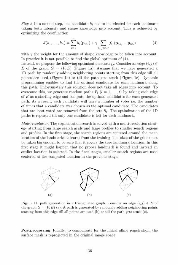
with γ the weight for the amount of shape knowledge to be taken into account.In practice it is not possible to find the global optimum of (4).Instead, we propose the following optimization strategy. Consider an edge (i, j) ∈E of the graph G = (V,E) (Figure 1a). Assume that we have generated a1D path by randomly adding neighboring points starting from this edge till allpoints are used (Figure 1b) or till the path gets stuck (Figure 1c). Dynamicprogramming enables to find the optimal candidate for each landmark alongthis path. Unfortunately this solution does not take all edges into account. Toovercome this, we generate random paths Pl (l = 1, . . . , t) by taking each edgeof E as a starting edge and compute the optimal candidates for each generatedpath. As a result, each candidate will have a number of votes i.e. the numberof times that a candidate was chosen as the optimal candidate. The candidatesthat are least voted are removed from the sets Si. The optimization of the 1Dpaths is repeated till only one candidate is left for each landmark.

Multi-resolution The segmentation search is solved with a multi-resolution strat-egy starting from large search grids and large profiles to smaller search regionsand profiles. In the first stage, the search regions are centered around the meanlocation of the landmarks as learnt from the training. The sizes of the grids mustbe taken big enough to be sure that it covers the true landmark location. In thisfirst stage it might happen that no proper landmark is found and instead anoutlier location is selected. In the finer stages, smaller search regions are usedcentered at the computed location in the previous stage.

(a) (b) (c)

Fig. 1. 1D path generation in a triangulated graph. Consider an edge (i, j) ∈ E ofthe graph G = (V, E) (a). A path is generated by randomly adding neighboring pointsstarting from this edge till all points are used (b) or till the path gets stuck (c).

Postprocessing Finally, to compensate for the initial affine registration, thesurface mesh is reprojected in the original image space.

138

3 Results

3.1 Parameter settings

For the morphological closing of the binary segmentations, a kernel of size 5 ×5 × 5 mm3 was used. The desired number of faces for the surface generationusing Amira [4] was set to 4000. The final landmark representation of the livercontained n = 2004 landmarks and t = 6000 edges.Two intensity models were built: one with profile radius r = 10 mm and one withr = 15 mm. Using the gaussian derivatives L,Lx, Ly, Lz with scales σ = 1, 2, 4voxels led to the generation of 24 feature images (see [8, 10] for more details).For the segmentation the following parameter settings were used. The numberof selected candidates per landmark was set to m = 100. This choice was led bycomputational aspects. During the optimization, the 20% least voted candidateswere removed in each iteration. Two multi-resolution stages were carried out.The first one with the profile r = 15 mm and the second with r = 10 mm.A proper choice for the weight γ was obtained by performing a leave-one-outsegmentation experiment on the training set. Table 1 shows the average distancemeasure between manual and automated segmentations for several choices of γ.The value of γ = 50 was selected to perform the segmentation of the test images.

γ = 5 γ = 10 γ = 20 γ = 50 γ = 100

Avg. Dist. [mm] 1.90 1.88 1.87 1.82 1.85Table 1. Tuning of the weight γ using a leave-one-out validation on the training set.The average distance between automated and ground truth segmentation is used ascriterium.

3.2 Testing Set

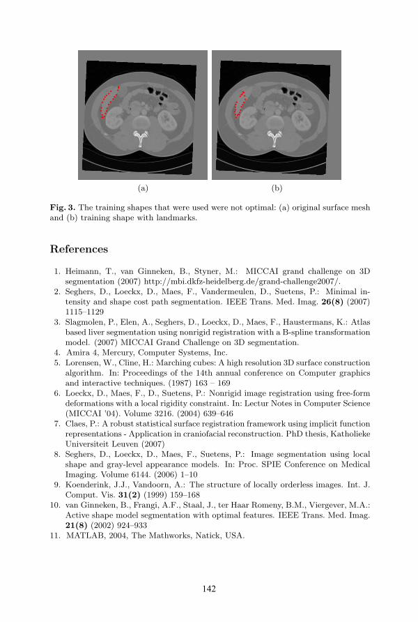
Table 2 and Figure 2 show the results of the segmentation method on the testimages. The method seems not to perform very well on most of the test images.When analyzing the results, two major problems were observed. First of all, itseemed that the wrong training meshes were used to build the model. To findcorresponding landmarks on the training shapes, two nonrigid registrations wereperformed (see section 2.1): (1) intensity registration and (2) point registration.Accidently, the shapes after only the first registration step were used to buildthe model. As a result, there was already a considerable error on the trainingshapes. An example of such an error is shown in figure 3. Obviously, this errordegenerates the intensity model.A second problem was observed when analyzing the result of case 4 (see Figure2, second row). The algorithm seemed to have missed the lower part of the liver.The reason for this error was that the search regions did not cover this part ofthe image. This kind of error did not happen for the leave-one-out experiment

139

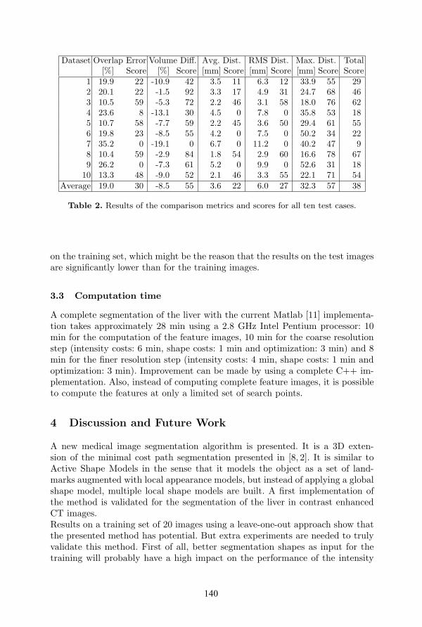
Dataset Overlap Error Volume Diff. Avg. Dist. RMS Dist. Max. Dist. Total[%] Score [%] Score [mm] Score [mm] Score [mm] Score Score

1 19.9 22 -10.9 42 3.5 11 6.3 12 33.9 55 292 20.1 22 -1.5 92 3.3 17 4.9 31 24.7 68 463 10.5 59 -5.3 72 2.2 46 3.1 58 18.0 76 624 23.6 8 -13.1 30 4.5 0 7.8 0 35.8 53 185 10.7 58 -7.7 59 2.2 45 3.6 50 29.4 61 556 19.8 23 -8.5 55 4.2 0 7.5 0 50.2 34 227 35.2 0 -19.1 0 6.7 0 11.2 0 40.2 47 98 10.4 59 -2.9 84 1.8 54 2.9 60 16.6 78 679 26.2 0 -7.3 61 5.2 0 9.9 0 52.6 31 18

10 13.3 48 -9.0 52 2.1 46 3.3 55 22.1 71 54Average 19.0 30 -8.5 55 3.6 22 6.0 27 32.3 57 38

Table 2. Results of the comparison metrics and scores for all ten test cases.

on the training set, which might be the reason that the results on the test imagesare significantly lower than for the training images.

3.3 Computation time

A complete segmentation of the liver with the current Matlab [11] implementa-tion takes approximately 28 min using a 2.8 GHz Intel Pentium processor: 10min for the computation of the feature images, 10 min for the coarse resolutionstep (intensity costs: 6 min, shape costs: 1 min and optimization: 3 min) and 8min for the finer resolution step (intensity costs: 4 min, shape costs: 1 min andoptimization: 3 min). Improvement can be made by using a complete C++ im-plementation. Also, instead of computing complete feature images, it is possibleto compute the features at only a limited set of search points.

4 Discussion and Future Work

A new medical image segmentation algorithm is presented. It is a 3D exten-sion of the minimal cost path segmentation presented in [8, 2]. It is similar toActive Shape Models in the sense that it models the object as a set of land-marks augmented with local appearance models, but instead of applying a globalshape model, multiple local shape models are built. A first implementation ofthe method is validated for the segmentation of the liver in contrast enhancedCT images.Results on a training set of 20 images using a leave-one-out approach show thatthe presented method has potential. But extra experiments are needed to trulyvalidate this method. First of all, better segmentation shapes as input for thetraining will probably have a high impact on the performance of the intensity

140

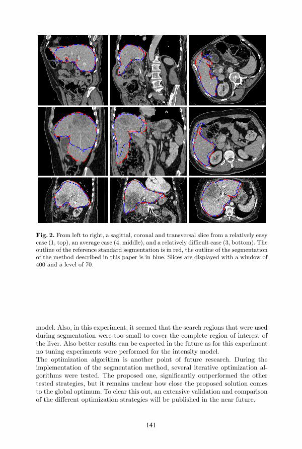
Fig. 2. From left to right, a sagittal, coronal and transversal slice from a relatively easycase (1, top), an average case (4, middle), and a relatively difficult case (3, bottom). Theoutline of the reference standard segmentation is in red, the outline of the segmentationof the method described in this paper is in blue. Slices are displayed with a window of400 and a level of 70.

model. Also, in this experiment, it seemed that the search regions that were usedduring segmentation were too small to cover the complete region of interest ofthe liver. Also better results can be expected in the future as for this experimentno tuning experiments were performed for the intensity model.The optimization algorithm is another point of future research. During theimplementation of the segmentation method, several iterative optimization al-gorithms were tested. The proposed one, significantly outperformed the othertested strategies, but it remains unclear how close the proposed solution comesto the global optimum. To clear this out, an extensive validation and comparisonof the different optimization strategies will be published in the near future.

141

(a) (b)

Fig. 3. The training shapes that were used were not optimal: (a) original surface meshand (b) training shape with landmarks.

References

1. Heimann, T., van Ginneken, B., Styner, M.: MICCAI grand challenge on 3Dsegmentation (2007) http://mbi.dkfz-heidelberg.de/grand-challenge2007/.

2. Seghers, D., Loeckx, D., Maes, F., Vandermeulen, D., Suetens, P.: Minimal in-tensity and shape cost path segmentation. IEEE Trans. Med. Imag. 26(8) (2007)1115–1129

3. Slagmolen, P., Elen, A., Seghers, D., Loeckx, D., Maes, F., Haustermans, K.: Atlasbased liver segmentation using nonrigid registration with a B-spline transformationmodel. (2007) MICCAI Grand Challenge on 3D segmentation.

4. Amira 4, Mercury, Computer Systems, Inc.5. Lorensen, W., Cline, H.: Marching cubes: A high resolution 3D surface construction

algorithm. In: Proceedings of the 14th annual conference on Computer graphicsand interactive techniques. (1987) 163 – 169

6. Loeckx, D., Maes, F., D., Suetens, P.: Nonrigid image registration using free-formdeformations with a local rigidity constraint. In: Lectur Notes in Computer Science(MICCAI ’04). Volume 3216. (2004) 639–646

7. Claes, P.: A robust statistical surface registration framework using implicit functionrepresentations - Application in craniofacial reconstruction. PhD thesis, KatholiekeUniversiteit Leuven (2007)

8. Seghers, D., Loeckx, D., Maes, F., Suetens, P.: Image segmentation using localshape and gray-level appearance models. In: Proc. SPIE Conference on MedicalImaging. Volume 6144. (2006) 1–10

9. Koenderink, J.J., Vandoorn, A.: The structure of locally orderless images. Int. J.Comput. Vis. 31(2) (1999) 159–168

10. van Ginneken, B., Frangi, A.F., Staal, J., ter Haar Romeny, B.M., Viergever, M.A.:Active shape model segmentation with optimal features. IEEE Trans. Med. Imag.21(8) (2002) 924–933

11. MATLAB, 2004, The Mathworks, Natick, USA.

142