Embed Size (px)
Citation preview
LAND USE AND VIOLENT CRIME
Thomas D. Stucky
John R. Ottensmann
School of Public and Environmental Affairs Indiana University Public Policy Institute
Indiana University–Purdue University Indianapolis Contact Information: Thomas D. Stucky, Ph.D. Associate Professor of Criminal Justice School of Public and Environmental Affairs BS/SPEA Building 4069 801 W. Michigan St. Indianapolis, IN 46202 [email protected]. 317-274-3462 (office) 317-274-7860 (fax) Keywords: land use, violent crime, spatial analysis, ecological theories
Brief biographical paragraphs John Ottensmann is a professor in the School of Public and Environmental Affairs at Indiana
University-Purdue University Indianapolis and serves as the director of urban policy research for the Center for Urban Policy and the Environment. He received his undergraduate degree from the University of Wisconsin at Madison and the Ph.D. in City and Regional Planning from the University of North Carolina at Chapel Hill. His research focuses on the spatial organization of urban areas, the spatial dimensions of public policy, and the use of analytical models to understand these issues. He has done applied public policy research for a variety of organizations and has published articles in a diverse range of scholarly and professional journals.
Thomas D. Stucky is Interim Director of Indiana University’s Center for Criminal Justice
Research and an Associate Professor of Criminal Justice. Professor Stucky earned his Ph.D. in Sociology at the University of Iowa in 2001. His scholarly interests are at the intersection of politics and criminal justice, specifically the relationship between politics and crime/policing at the city level, and state level trends in imprisonment and correctional spending. He is also interested in the continuing development of the systemic social disorganization theory, and among other things the relationship between land use, the physical environment and crime. He has authored two books, and journal articles appearing in Criminology, Journal of Quantitative Criminology, Journal of Research in Crime and Delinquency, and Justice Quarterly, among others.
This is the author's manuscript of the article published in final edited form as: Stucky, T. D., & Ottensmann, J. R. (2009). Land Use And Violent Crime*. Criminology,
47(4), 1223-1264. http://dx.doi.org/10.1111/j.1745-9125.2009.00174.x
1

LAND USE AND VIOLENT CRIME
Although research has shown specific land uses to be related to crime, systematic
investigation of land uses and violent crime has been less common. This study systematically
examines links between land uses and violent crime and whether such links are conditioned by
socioeconomic disadvantage. We employ geocoded UCR data from the Indianapolis police
department and information on 30 categories of land use, and demographic information from the
2000 census. We use land use variables to predict violent crime counts in 1000 X 1000 feet grid cells
using negative binomial regression models. Results show that, net of other variables, specific land
uses predict variation in counts for individual violent crimes and aggregate rates. Some
nonresidential land uses are associated with higher violent crime counts, whereas others are
associated with lower counts. Specific land uses also condition the effects of socioeconomic
disadvantage on violent crime. Implications for routine activities/opportunity and social
disorganization/collective efficacy theories of crime are discussed.
2
INTRODUCTION
Consideration of the relationship between land use and crime has a long history in
criminological research, dating back at least to the early studies in the Chicago school (Burgess,
1916; Shaw and McKay, 1972[1942]). Land uses are discussed in a variety of lines of research
including Jacobs’ (1961) and Newman’s (1971) early work on urban landscapes and crime,
Brantingham and Brantingham’s (1981) crime pattern theory, routine activities/opportunity theories
(Cohen and Felson, 1979; Kennedy and Forde, 1990), hot spots research (Loukaitou-Sideris, 1999;
Sherman, Gartin, and Buerger, 1989; Weisburd, Bushway, Lum, and Yang 2004), and research on
crime prevention through environmental design (CPTED) (Eck, 2002; Felson, 2002; Jeffrey, 1976,
1977; Lab, 1992; Plaster-Carter, Carter, and Dannenberg, 2003).1
Despite this longstanding, periodic attention to land use (Duffala, 1976; Fowler, 1987;
Greenberg and Rohe, 1984; Greenberg, Rohe, and Williams, 1982; Ley and Cybriwsky, 1974;
Lockwood, 2007; Smith, Frazee, and Davidson, 2000; White, 1932; Wilcox, Quisenberry, Cabrera,
and Jones 2004), until recently it has not figured prominently in research on several mainstream
ecological theories. Thus, land use is completely absent from anomie/strain research and most tests
of social disorganization/collective efficacy theories (but see Sampson and Groves 1989).2
Research also frequently focuses on a few specific land uses such as taverns (Roncek and
Maier, 1991; Roncek and Pravatanier, 1989) or schools (LaGrange, 1999; Roncek and Faggiani,
1985; Roncek and LoBosco, 1983), or combines land use information into indices (McCord,
Ratcliffe, Garcia, and Taylor 2007; Wilcox et al., 2004), or single measures of “mixed” or
nonresidential land use. For example, Sampson and Raudenbush (1999) include a measure of “mixed
land use” but find no effects of the measure on crime, whereas Cahill (2005) finds significant effects
of mixed land uses on crime. These conflicting findings may result from treating different land uses
1 See also Murray (1983), Roncek (1981), Taylor (1998), Taylor and Gottfredson (1986), Taylor and Harrell (1996) for overviews of physical environment and crime. 2 See Brantingham and Jeffrey (1981) for a discussion of this issue with respect to social disorganization theory.
3
similarly. If not all land uses produce crime, then combining such measures risks masking potentially
opposite effects on crime. For example, commercial establishments may be associated with higher
crime because they place potential offenders and targets in proximity with regularity. But do
industrial areas, which likely place fewer offenders and targets in proximity, also create similar
opportunities for crime? To date, few studies have systematically examined links between particular
land uses and violent crime.3
Many studies have assumed that land uses have direct effects on crime irrespective of social
context. Thus, the effect of “nonresidential” land uses is expected to be the same in advantaged or
disadvantaged areas. Such an assumption seems unwarranted because the potential for land uses to
create opportunities for crime likely depends on the willingness and/or capacity of occupants of an
area to exercise social control (see Merry, 1981; Smith, Frazee, and Davison, 2000; Wilcox et al.,
2004), which are also likely to vary based on the relative advantage or disadvantage of a
neighborhood. Thus, a few recent studies have argued that the effects of land uses on crime are likely
conditional on the socioeconomic characteristics of the area (Smith et al., 2000; Wilcox et al., 2004).
Yet, these studies considered a limited number of land uses, and either focused on a single crime, or
employed subjective land use measures. Therefore, additional systematic consideration of the
conditional effects of land use and socioeconomic disadvantage seems warranted. The current study
advances research on land use by systematically exploring whether and how a wide variety of
objectively-measured land uses and several violent crimes are related, and by exploring whether land
uses and socioeconomic disadvantage have independent or conditional effects on violent crime.
Following a discussion of existing research on land use and crime, we discuss the data and methods
used in the current study. Then we discuss the results of negative binomial analyses of the links
between land uses, socioeconomic and demographic factors, and geocoded UCR violent crime counts
3 Several recent studies have examined links between land uses, neighborhood deterioration, and actual or perceived disorder such as Kurtz, Koons, and Taylor (1998); McCord et al., (2007); Taylor, Koons et al., (1995); Wilcox, Quisenberry, and Jones (2003).
4
in 1000 X 1000 feet square grid cells in Indianapolis, Indiana. We close by discussing the
implications of the current study for systemic social disorganization/collective efficacy and routine
activities/opportunity theories of crime.
LAND USE AND CRIME
Although studies of land use have appeared sporadically for decades, there appears to be a
renewed attention to land use in recent years. Recent studies have focused on land use, usually from
two broad perspectives—routine activities/opportunity theories and social disorganization/collective
efficacy theories.4 Developed in 1979 by Cohen and Felson, routine activities theory suggests that the
daily activities in which citizens engage—going to work, school, and church—differentially place
potential offenders and potential targets in close proximity, which leads to variation in crime
victimization. From this perspective, a crime is more likely to the extent that motivated offenders and
suitable targets meet in the absence of a capable guardian. Thus, studies incorporating land use have
focused on how particular land uses such as bars (Roncek and Maier, 1991; Roncek and Pravatanier,
1989) or schools (LaGrange, 1999; Roncek and Faggiani, 1985; Roncek and LoBosco, 1983) can
increase crime by regularly placing offenders and victims in proximity in the absence of
guardianship. For example Roncek and Maier (1991) found that areas with bars tend to have higher
violent and property crime (UCR index offenses), net of sociodemographic factors. Similarly,
LaGrange (1999) examined the effects of malls and schools on minor crimes for a one-year period in
Alberta, Canada, from a routine activities perspective. She argued that schools and malls place many
people who don’t know each other (malls) or are at a crime prone age (schools) together. Using data
“enumeration areas” (subunits of census tracts) from Edmonton, LaGrange found that malls and
public high schools, rental units, rooming houses, and vacant lots all increase criminal mischief and
damage to parks and transit areas.
The opportunity approach suggests that different land uses are likely to create different
4 One recent study (McCord et al., 2007) focuses on Brantingham and Brantingham’s crime pattern theory.
5
opportunity structures for crime, by influencing the mix of motivated offenders, potential victims,
and the presence or absence of capable guardians. So a church is likely to create a very different set
of social interactions that seems much less likely to place offenders and victims in proximity (in the
absence of guardianship) than commercial activities. Yet, as noted above, many studies create
aggregate measures of land uses as if all nonresidential land uses can be assumed to similarly
increase opportunities for crime (Cahill, 2005; Sampson and Raudenbush, 1999) or focus on a few
specific land uses (LaGrange, 1999; Roncek and Faggiani, 1985; Roncek and LoBosco, 198l; Roncek
and Maier, 1991; Roncek and Pravatanier, 1989). Therefore, a study which allows for investigation
of the independent effects of a variety of land uses is warranted.
Other recent studies of land use and crime have employed the social disorganization/
collective efficacy perspective. Developed from the Chicago School tradition and Shaw and Mckay’s
landmark study (1972 [1942]), social disorganization theory posits that community crime rates vary
because social structural factors such as poverty, ethnic heterogeneity, and family instability, impede
the ability of residents to maintain informal social control in the neighborhood (see also Bursik,
1988; Sampson and Groves, 1989). Although most social disorganization studies focus on social
ecology, some studies also consider land uses (Lockwood, 2007; Sampson and Raudenbush, 1999;
2000; Wilcox et al., 2004). Some argue that mixed or nonresidential land uses impede the ability of
residents to maintain social control by increasing street traffic which increases the number of
strangers in an area and reducing residents’ ability to tell locals from outsiders (Gardiner, 1976;
Greenberg, Rohe, and Williams, 1982; Kurtz, Koons, and Taylor, 1998; Taylor et al., 1995; Wilcox
et al., 2004), or by increasing actual or perceived neighborhood deterioration, disorder, or incivilities
(Kurtz et al. 1998; McCord et al., 2007; Taylor et al., 1995; Wilcox, Quisenberry, and Jones 2003).5
5 Others argue that mixed land uses can be beneficial. Jacobs (1961) argued that mixed land uses are crucial because they keep people in areas throughout a day. Thus, there are constantly “eyes on the street.” Expanding on Jacobs’ work, Newman (1972) developed the concept of ‘defensible space.’ Newman suggested that territoriality (the degree to which an area appears to be “owned”) and natural surveillance are factors that would likely affect an offenders’
6
Consistent with this logic, Lockwood (2007) examines the influences of retail/commercial and
public/institutional, and recreational land uses on robbery, aggravated assault, and simple assault
rates in 145 census block groups in Savannah, Georgia. Lockwood (2007) finds that both commercial
and public land uses are significantly positively associated with simple assault, aggravated assault,
and robbery rates. 6 Additionally, the author finds that recreational land uses are significantly
positively associated with robbery rates. Yet, Lockwood’s analysis focuses only on a few very broad
categories of land uses, the study has a small sample size, and the study only considers direct effects
of land uses on crime.
Recently, theorists have begun to suggest combining social disorganization and routine
activities theories (Smith et al., 2000). Such an approach would suggest that crime rates will vary
based both on how frequently routine daily activities place offenders and targets in proximity, and
the willingness or capacity of others to intervene to maintain social control.
Consistent with this logic, two recent studies have suggested that the effect of land uses on
crime may be conditional on the socioeconomic characteristics of the neighborhood. If
socioeconomic disadvantage (a structural antecedent of social disorganization) is generally
associated with lesser levels of informal social control, ceteris paribus, then the crime generating
potential of land uses will likely vary depending on the level of disadvantage in an area. Consistent
with this, Smith et al. (2000: 516) found that “[s]ocial disorganization attributes of a face block
combine with land use factors to affect the probability that street robbery will occur.” Specifically,
the authors found that the influence of hotels/motels, and bars/restaurants/gas stations on robbery was
greater as the number of single parent households in a face-block increased, whereas the influence of
choice of whether or not to commit a crime in a given area. He argued that physical characteristics can give the impression that space will be defended and therefore reduce the likelihood of crime. In addition, if people feel they own a space, they will be more likely to exercise informal social control over it and as a result, crime will be lower. Evidence on the utility of defensible space is mixed (Mawby, 1976; Merry, 1981; Taylor, Gottfredson, and Brower, 1980, 1984). 6 The author also noted having examined homicide rates but no results were presented for these analyses.
7
multifamily structures, bars/restaurants/gas stations, and vacant/park lots on robberies decreased with
distance from the center of the city. Although promising, these findings are specific to robbery and
include primarily commercial kinds of land uses.
Similarly, Wilcox et al. (2004) suggest that the effect of land use on crime might be
conditional on the socioeconomic characteristics of the area (see also Wilcox, Quisenberry, and
Jones, 2003). Wilcox et al. (2004) examined the linkages between specific land uses and burglary,
assaults, and robberies in 100 Seattle neighborhoods. The authors argued that certain types of land
use will lead to greater difficulty in maintaining informal social control because of the greater
amount of “public” space and the larger number of strangers. Wilcox et al. (2004) also argued that
certain types of land use are more likely to be associated with physical deterioration or incivilities,
which could lead to more serious crimes (i.e., broken windows logic). The authors found that the
effects of businesses on burglary and playgrounds on robberies and assaults were conditional on the
relative level of population instability. Yet, the effects ran counter to their expectations. Wilcox et al.
(2004) had predicted that some land uses would be more likely to be associated with crime in
unstable areas. Their analyses showed just the opposite to be true. They speculate that such land uses
in unstable areas may encourage greater monitoring by parents at playgrounds and the police or
business owners for businesses in unstable areas. Yet, this study only considered a few land uses,
relied on a small number of census tracts, did not control for crime or disadvantage in surrounding
areas, and employed subjectively determined land use measures.7
In sum, although land use measures have periodically been incorporated in criminological
studies, most studies have assumed that nonresidential land uses independently increase opportunities
or decrease the potential for informal social control. Recently, authors have suggested that
opportunity and informal social control may have conditional effects on crime. Consistent with this
7 Respondents were asked a series of questions regarding the presence of nine land uses within three blocks of their homes.
8
logic, two recent studies (Smith et al., 2000; Wilcox et al., 2004) have considered conditional effects
of land uses and disadvantage on violent crime. Yet, each has limitations that suggest the need for
additional research. Therefore, a systematic study of the effect of objectively-measured land uses on
a variety of serious violent crimes that considers the conditional effects of land uses and disadvantage
seems warranted.
DATA AND METHODS
The data for this study come from three sources, the Indianapolis Police Department (IPD)
Uniform Crime Report (UCR) data for 2000-2004, land use data from the Indianapolis Department of
Metropolitan Development from 2002, and 2000 Census data.8 Crime data for the study covers the
IPD service area, which is approximately the Indianapolis city boundaries before city-county
consolidation in 1970.9
UNIT OF ANALYSIS
The units of analysis for this study are 2,142 1000-feet square grid cells overlaid on the (IPD)
service area. Grid cells only partially included within the boundaries have been excluded from the
analysis because only some crimes in them would have been reported to IPD. One advantage of this
approach is that the grid cells are much more homogeneous than larger units such as census tracts or
block groups. Although other units such as census blocks or face blocks (e.g. Smith et al., 2000)
might have been chosen, each would present significant problems for allocating the crime data (See
Appendix 1 for additional discussion of the use of grid cells rather than census-based boundaries).
Maps 1 and 2 illustrate the IPD service area relative to Marion County, Indiana, and the grid cell
approach taken in the current analysis.
Maps 1 and 2 about here
8 Although these data could be subject to concerns over causal order, it seems unlikely that in the short run changes in crime are unlikely to cause changes in land use. 9 The 2000 population of the IPD service area was 322,212. This population is comparable to that for other large central cities in the Midwest, such as Pittsburgh, PA (334,563), Cincinnati, OH (331,285), and St. Louis, MO (348,189).
9
DEPENDENT VARIABLES
In this analysis, we use geocoded UCR data for the IPD service area from 2000-2004 to
examine the violent index offenses (murder and non-negligent manslaughter, rape, robbery,
aggravated assault) individually and as a violent crime index.10 We focus on violent crimes because,
by definition, these require an offender and a target to interact. For each crime, the count of incidents
per cell was determined. The crime locations were geocoded from address information, so that
crimes could be located as accurately as the nearest street address.11
SOCIOECONOMIC VARIABLES
To determine whether land uses influence crime net of socioeconomic variables, and whether
their influence on crime is conditioned by disadvantage, it is necessary to control for relevant
socioeconomic predictors of violent crime. Therefore, we include the socioeconomic characteristics
of the areas in which each of the grid cells are located. Values of the sociodemographic variables
have been estimated for each grid from the 2000 census. To estimate the grid cell values the blocks
and census tracts were intersected with the grid cells and the values of blocks and tracts split by the
grid cells were apportioned to the cells based on the proportion of the area of the block or census
tract within the cell. Block data from Summary File 1 were used for the estimation of those
10 The homicide variable includes homicides from 1992 to 2004 to increase stability of estimates. Preliminary analyses also considered homicides from 2000 to 2004 with similar results. 11 IPD did not provide information on the geocoding success rate for the UCR data that were provided or describe the geocoding procedures used. However, the dataset included a small number of records (less than 1%) for which no geocoded coordinate information was provided. Some of these records included “UNKNOWN” in the address field, while others included addresses that apparently could not be successfully geocoded. Based upon this, one might infer that the geocoding success rate exceeded 99 percent, though we cannot definitively conclude this, which would be a very high success rate. IPD uses the street database of the Metropolitan Emergency Communications Agency, which handles 911 dispatching for geocoding. This is an extremely comprehensive and accurate database, which would contribute to a very high geocoding success rate. Further, IPD has full-time personnel devoted to “cleaning” the UCR data and puts considerable effort into the UCR dataset so that the crime locations accurately reflect the locations of the crimes as opposed to the locations to which the officers initially responded. This is evidenced by the time delays associated with the release of the UCR data. While IPD makes their officer incident report data available within 24 hours, the UCR data are not available until approximately 4-5 months later. This suggests attention to developing accurate address information that could make the high geocoding success rate plausible.
10
characteristics reported at the block level: population, Hispanic population, African-American
population (all persons reporting at least one race African-American), number of female headed
households, number of occupied housing units, and number of owner-occupied housing units.
Block group data from Summary File 3 were used for the estimation of those characteristics
obtained from the long-form (sample) questions: population change from 1990 to 2000, number of
persons foreign born, number of persons aged 16 and over in civilian labor force, number of
employed persons, number of persons for whom poverty status was determined, and number of
persons below the poverty level. It should be noted that there can be a number of grid cells in each
block group in some cases (see Map 3). Therefore, because these block group characteristics
represent an aggregation across the area within each block group, the much smaller grid cells may in
some cases depart from this average.
Previous research has shown that many social structural predictors of crime such as poverty,
unemployment, and family disruption are often highly correlated. Therefore, following previous
research (Land, McCall, and Cohen, 1990; Parker and McCall, 1999), using principal components
analyses, we created a disadvantage index which included the following indicators: percent poor,
percent unemployed, median household income, and percent female-headed households. Factor
loadings ranged from 0.68 to 0.83. Social disorganization theory and research has focused on the
difficulty of maintaining social control in unstable neighborhoods (Wilcox et al., 2004). Therefore,
we developed a stability index, consisting of the percent of housing units that were owner-occupied,
the percent that is foreign born, and the percent of the population that had not moved for five years.12
Factor loadings on this index ranged from 0.66-0.82. In addition, the percentage of the population
that is African American and the percentage Hispanic in the cell are included. To control for the
12 Alternative specifications that included only the percent of owner-occupied residents or percent of population that had not moved in the previous five years produced similar results to those reported in tables 2 and 3.
11
possibility that greater counts of violent crime will occur in a cell simply because more people live in
an area, we control for the cell population (Land et al. 1990).
LAND USE VARIABLES
Prior research has considered several land use categories. The land use data available for
Indianapolis included parcel-based data on land use in 2002 obtained from the Indianapolis
Department of Metropolitan Development. Each parcel was assigned a land use in one of the
following categories: Residential (0 – 1.75, 1.76 – 3.5, 3.6 – 5, 5.1-8, 8.1-15, over 15) units per acre,
Commercial (office, retail/ community, heavy, downtown mixed), Vacant, Agriculture,
Industrial (light, heavy), Hospitals, Schools, Cemeteries, Churches, Utilities, Parks, Water, Unknown
or under development, Village mixed use, Airport-related mixed use. Land use parcel information
was intersected with the grid cells to obtain the portions of each parcel within each grid cell and
summarized to produce the total area of the land in each grid cell devoted to each land use type. Then
for each land use type, the percentage of the land area of the grid cell in the land use type was
determined.
Preliminary analyses examined both presence of land use and the percentage of the cell
devoted to each land use. Following extensive examination of land uses empirically and through
review of previous research, the following set of land uses were included in the models described
below.13 Consistent with prior research suggesting that schools can be associated with higher crime,
we include a categorical variable to indicate the presence of a school land use in the cell. Categorical
variables were included for the presence of hospitals and cemeteries. If nonresidential land uses are
associated with higher crime, one might expect that hospitals would be associated with higher crime
because they bring many strangers together. Conversely, cemeteries could be associated with fewer
violent crimes because they are unlikely to place offenders and targets in proximity.
13 All land use percentage variables were expressed as a percentage of the total non-road land use with the exception of the residual land use variable which was expressed as a percentage of the total area of the cell.
12
Examination of prior research suggests that commercial businesses are likely to be associated
with higher crime (Smith et al., 2000) by frequently placing offenders and targets in proximity.
Likewise, vacant land has been posited to be associated with higher crime (Greenberg et al., 1982;
LaGrange, 1999; Ley and Cybriwsky, 1974), presumably through increased opportunity in the
absence of guardianship or informal control. Although some have argued that industry, as a
nonresidential land use, could be associated with higher crime (Lockwood, 2007), others suggest that
industry might be associated with lower crime (Felson, 1987). In addition, some studies have found
parks or recreational land uses to be associated with crime (Lockwood, 2007; Wilcox et al., 2004).
Although, not studied in other research that we are aware of, water is a feature of many cities,
whether in the form of rivers, lakes, or retention ponds. We anticipate that water would reduce the
opportunity for violent crimes, although the areas around water may be areas with lower
guardianship or informal social control.14 To explore these effects individually, commercial
businesses, industry, vacant land, parks, and water land uses were all included and expressed as
percentages of the total land area in each cell.15
Some studies have also shown that high density housing can create anchors for disadvantage
and crime (McNulty and Holloway, 2000). Therefore, a categorical variable was also created to
capture the presence of high density residential land use within a cell (defined as 8 or more units per
acre). Additionally, the presence of through traffic streets may increase crime by increasing street
traffic and the presence of strangers (Greenberg et al., 1982). Therefore, we include a continuous
variable that captures the sum total of the length of major roads in each grid cell. Thus, if a cell had
one major road running through the entire cell, the value of the variable would be 1000.
14 One reviewer suggested that we examine buffers around water because beaches may bring large numbers of people together and increase opportunities for crime. We agree that this would be appropriate in some areas, however, in our study there are no large bodies of water with beaches. 15 Despite the ability to examine many specific land uses, data were limited in some ways. In the dataset, there were four broad categories of commerce that provided no opportunity for further disaggregation. Thus, in this study we are unable to distinguish taverns from other commercial establishments.
13
Finally, we include a variable that captures the percentage of remaining land uses as a control
variable. This residual land use variable includes the percentage of total land area devoted to
agriculture, utilities, railroad rights-of-way, rights-of-way, village or airport mixed uses, under
development, other, and unknown.16 (See table 1 for variable means and standard deviations and
Appendix 2 for variable correlations.)
Table 1 about here
MODELING STRATEGY
Perhaps not surprisingly due to the size of the grid cells, the distribution of the dependent
variable is highly skewed. Especially for homicide and rape, many cells have zero counts. Therefore,
a Poisson distribution is more appropriate for count data (Greene, 2000; Osgood, 2000, Osgood and
Chambers, 2000). Because Poisson models assume that there is no residual dispersion left to explain
once the explanatory variables are included, we employ negative binomial models (which include a
dispersion parameter) in the analyses reported below.17 We limited the analysis to cells with a
population count greater than zero. Combined with missing information on some independent
variables for some cells, this caused a 7.7% reduction in the sample size from 2,142 to 1,956.
Because cells can be contiguous, the crime data can be expected to exhibit spatial
autocorrelation, producing spatially correlated errors in the normal negative binomial models.
Indeed, calculation of a Moran’s (1948) I statistic for all crimes discussed below confirmed
statistically significant (p <.001) spatial auto-correlation.18 To address this, we develop spatial
autoregressive models by including a spatial lag variable in the model (Fotheringham, Brunsdon and
16 We are grateful to anonymous reviewers for this suggestion. 17 The advantage of including this parameter in the model is that when there is no over-dispersion in the model, the parameter estimate is 0 and the negative binomial model reduces to the Poisson model. 18 The Moran’s I statistic was calculated using Anselin’s GeoDa version 0.9.5-i. Significance was calculated using the random permutation procedure with 999 permutations. Results were substantively similar using the Queen or Rook contiguity.
14
Charlton, 2000). For the weight matrix, we include the eight adjacent cells surrounding each grid
cell, producing a spatial lag variable that is the average of the counts for the specific crime in those
adjacent cells.19 The multivariate models reported in tables 2 and 3 were estimated using maximum
likelihood methods in SAS Proc Genmod.
RESULTS
BIVARIATE RESULTS
To determine whether land use and crime are related, it seems reasonable to examine the data
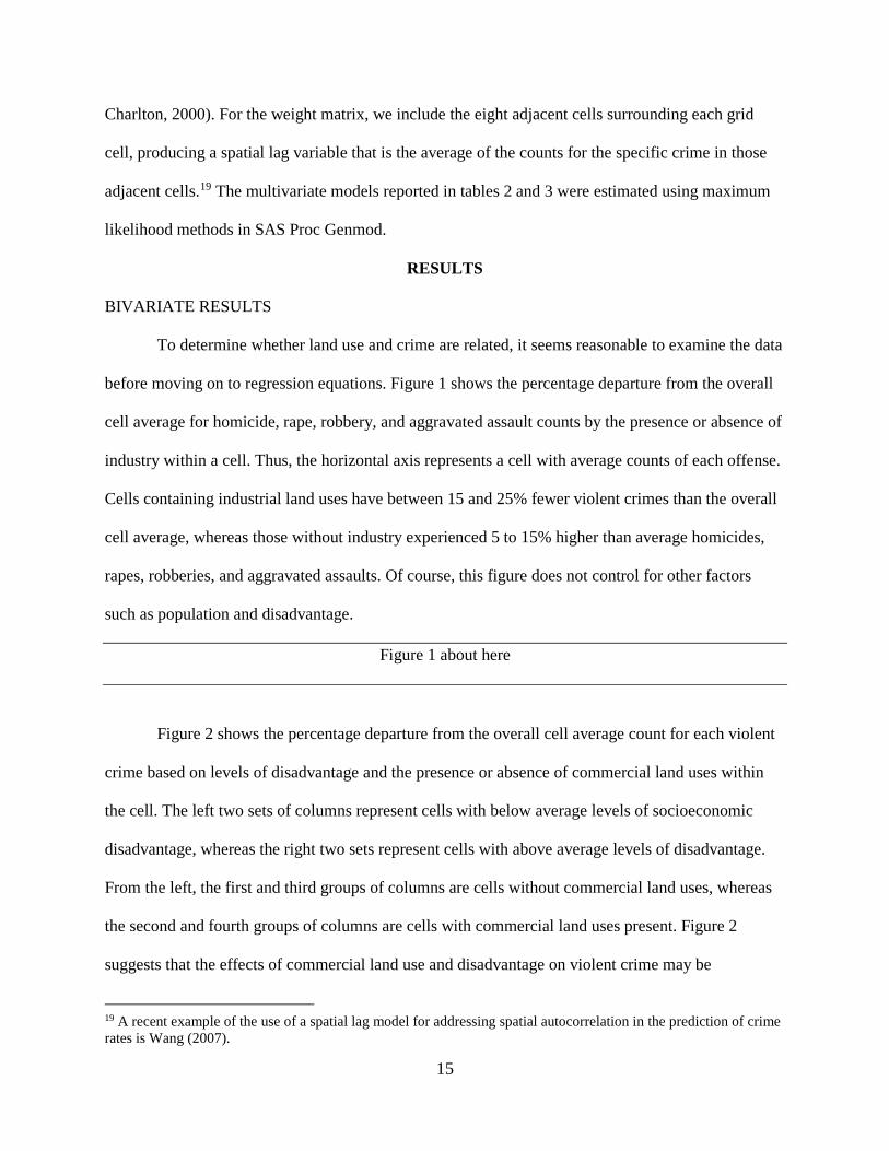
before moving on to regression equations. Figure 1 shows the percentage departure from the overall
cell average for homicide, rape, robbery, and aggravated assault counts by the presence or absence of
industry within a cell. Thus, the horizontal axis represents a cell with average counts of each offense.
Cells containing industrial land uses have between 15 and 25% fewer violent crimes than the overall
cell average, whereas those without industry experienced 5 to 15% higher than average homicides,
rapes, robberies, and aggravated assaults. Of course, this figure does not control for other factors
such as population and disadvantage.
Figure 1 about here
Figure 2 shows the percentage departure from the overall cell average count for each violent
crime based on levels of disadvantage and the presence or absence of commercial land uses within
the cell. The left two sets of columns represent cells with below average levels of socioeconomic
disadvantage, whereas the right two sets represent cells with above average levels of disadvantage.
From the left, the first and third groups of columns are cells without commercial land uses, whereas
the second and fourth groups of columns are cells with commercial land uses present. Figure 2
suggests that the effects of commercial land use and disadvantage on violent crime may be
19 A recent example of the use of a spatial lag model for addressing spatial autocorrelation in the prediction of crime rates is Wang (2007).
15
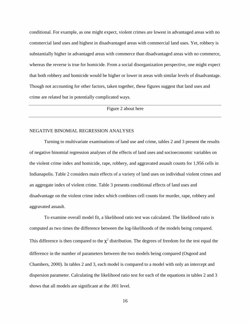
conditional. For example, as one might expect, violent crimes are lowest in advantaged areas with no
commercial land uses and highest in disadvantaged areas with commercial land uses. Yet, robbery is
substantially higher in advantaged areas with commerce than disadvantaged areas with no commerce,
whereas the reverse is true for homicide. From a social disorganization perspective, one might expect
that both robbery and homicide would be higher or lower in areas with similar levels of disadvantage.
Though not accounting for other factors, taken together, these figures suggest that land uses and
crime are related but in potentially complicated ways.
Figure 2 about here
NEGATIVE BINOMIAL REGRESSION ANALYSES
Turning to multivariate examinations of land use and crime, tables 2 and 3 present the results
of negative binomial regression analyses of the effects of land uses and socioeconomic variables on
the violent crime index and homicide, rape, robbery, and aggravated assault counts for 1,956 cells in
Indianapolis. Table 2 considers main effects of a variety of land uses on individual violent crimes and
an aggregate index of violent crime. Table 3 presents conditional effects of land uses and
disadvantage on the violent crime index which combines cell counts for murder, rape, robbery and
aggravated assault.
To examine overall model fit, a likelihood ratio test was calculated. The likelihood ratio is
computed as two times the difference between the log-likelihoods of the models being compared.
This difference is then compared to the χ2 distribution. The degrees of freedom for the test equal the
difference in the number of parameters between the two models being compared (Osgood and
Chambers, 2000). In tables 2 and 3, each model is compared to a model with only an intercept and
dispersion parameter. Calculating the likelihood ratio test for each of the equations in tables 2 and 3
shows that all models are significant at the .001 level.
16
Table 2 about here
Turning to the effects of individual variables, as one might expect, in all equations in table 2,
the spatial lag variable is significant, showing that violent crime is positively correlated with violent
crime in adjacent cells. Population size is also significantly positively related to all violent crimes for
all equations, and the percentage of the population in the cell that is African American is significantly
positively associated with all violent crimes except rape. The percentage of the population that is
Hispanic in the cell is significantly positively related to the violent crime index, aggravated assault,
and homicide, but not rape or robbery. The index of population stability is significantly negatively
related to all violent crimes except robbery (p <.10 for homicide).20 Consistent with prior research,
the socioeconomic disadvantage index is significantly positively related to all violent crimes in table
2 (p <.001). However, as we will see in table 3, the effects of socioeconomic disadvantage on violent
crime are conditioned by certain land uses.
Table 3 about here
Turning to the effects of specific land uses on violent crime, the presence of high density
residential units in the cell (8 or more units per acre) was significantly positively (p<.001) associated
with all violent crimes in table 2, even controlling for population size and socioeconomic
disadvantage. There appears to be something about such units that is associated with all types of
serious violent crime, even controlling for the other factors in the model. Apparently high density
housing units promote serious violent crime.
The percent of a cell devoted to commerce is significantly positively related to all crimes in
table 2 except homicide, even net of the other factors in the model. From a routine activities
20 We tested numerous interaction effects with land use variables and the stability index but none were significant.
17
perspective, one would expect this result because commercial activities increase the frequency of
offender and target contacts in the absence of capable guardians, ceteris paribus. The percentage of a
cell devoted to industry is significantly negatively related to the violent crime index, robberies, and
aggravated assaults, marginally negatively related to rape (p<.10), but is unrelated to homicide in
table 2. Although some would suggest that all nonresidential land uses are associated with higher
crime, these results suggest that this is not always the case. From the routine activities perspective
(Felson, 1987), these results make sense because industrial areas are not likely to attract large
numbers of potential offenders, although they are not likely to be areas where large numbers of
capable guardians are present. Although to our knowledge, no research has considered whether water
and crime are related, we included water to be systematic. The percent of water in a cell was
significantly negatively related to the violent crime index, robbery, and aggravated assault (p <.05),
but unrelated to homicide or rape. This suggests that water in an area decreases the number of violent
crimes, most likely by decreasing the opportunities for offenders and victims to interact. We also
examined whether the length of major streets in the cell influenced violent crime, net of the other
factors in the model. As expected, we found that the lengths of major streets in a cell were
significantly positively associated with violent crime overall and individually in all equations in table
2. Additional major streets likely increase the number of strangers in an area, and, ceteris paribus,
increase the number of potential offenders and victims in an area, which may also make it more
difficult to maintain informal social control. Additional major streets also increase the number of
entry and exit points, which may make areas more attractive for offenders (see White, 1990 for a
discussion of research on neighborhood permeability).21
21 We also considered a binary variable indicating the presence of major streets and a continuous variable that captured the total percentage of the land in a cell devoted to streets, highways, and interchanges. Both alternative specifications produced similar main and interaction effects to those reported in tables 2 and 3. We are grateful to anonymous reviewers for suggesting alternative specifications to probe the robustness of this relationship.
18

The presence of a cemetery in the cell was significantly negatively related to homicide and
robbery (p<.05), and marginally negatively related to the violent crime index (p<.10). Thus, it
appears that cemeteries reduce some kinds of crime, possibly by suppressing the number of potential
offender-victim interactions. School land use was significantly negatively related to homicide
(p<.05), and marginally negatively related to rape (p<.10), but unrelated to robbery, aggravated
assault, or the violent crime index. These mixed findings contradict prior studies that have shown
schools to be related to crime. Perhaps the explanation lies in a limitation of the current data. School
land use includes all types of educational institutions, including public and private elementary and
secondary schools and colleges and universities. Presumably public high schools might be more
likely to be related to serious violent crimes than private elementary schools.
The presence of a hospital in a cell was also unrelated to violent crime in all equations in
table 2. We had expected that hospitals might attract both offenders and victims and therefore
increase the potential for violent crimes. Yet, unlike commercial areas, hospitals do not appear to be
associated with violent crime. In addition, contrary to some prior studies (Lockwood, 2007; Smith et
al., 2000), the percent of a cell devoted to park related land use was significantly negatively
associated with aggravated assault (p <.01) and marginally negatively related to homicide (p < .10),
but unrelated to the other violent crimes in table 2. Such a finding is somewhat surprising because
one might expect parks to increase interactions between potential offenders and targets, in the
absence of guardians and be areas where informal social control would be lower. Finally, the percent
of vacant land in a cell was marginally positively related to robbery in table 2 (p < .10) but unrelated
to the other crimes. One explanation for this may be that in this context, vacant land means that there
is no structure on the land, which can mean very different things depending on the context
surrounding the vacant land. Thus, a vacant lot in a brand new subdivision is likely to have very
different implications for violent crime than a vacant lot surrounded by boarded up buildings.
19
Finally, the residual land use category that we included was significantly negatively associated with
the violent crime index, aggravated assault, and robbery, but not rape or homicide.22
THE CONDITIONAL EFFECTS OF LAND USE AND DISADVANTAGE ON VIOLENT CRIME
Table 3 considers whether the influences of land uses and disadvantage on violent crime are
conditional. To avoid reporting on multiple analyses, we limit these analyses to the overall violent
crime index and those results where there were consistent interactions between land uses and
disadvantage (although numerous other interaction terms were examined). In general, the main
effects of the control variables on violent crime are consistent with expectations and remarkably
stable across the five equations reported in table 3. Specifically, the spatial lag variable, cell
population, socioeconomic disadvantage, percent Black and percent Hispanic are all significantly
positively related to the violent crime index, and the stability index is significantly negatively related
to violent crime in all equations as expected (disadvantage is marginally significant in equation 1). In
addition, the main effects for several land uses including high density housing, percent commercial,
percent industrial, percent water, and the binary variable for the presence of a cemetery and the
length of major streets variable achieve significance in all equations in table 3, and are in the
expected direction. Parks, schools, hospitals, and the percentage of vacant land in a cell were
unrelated to the violent crime index in all equations in table 3.
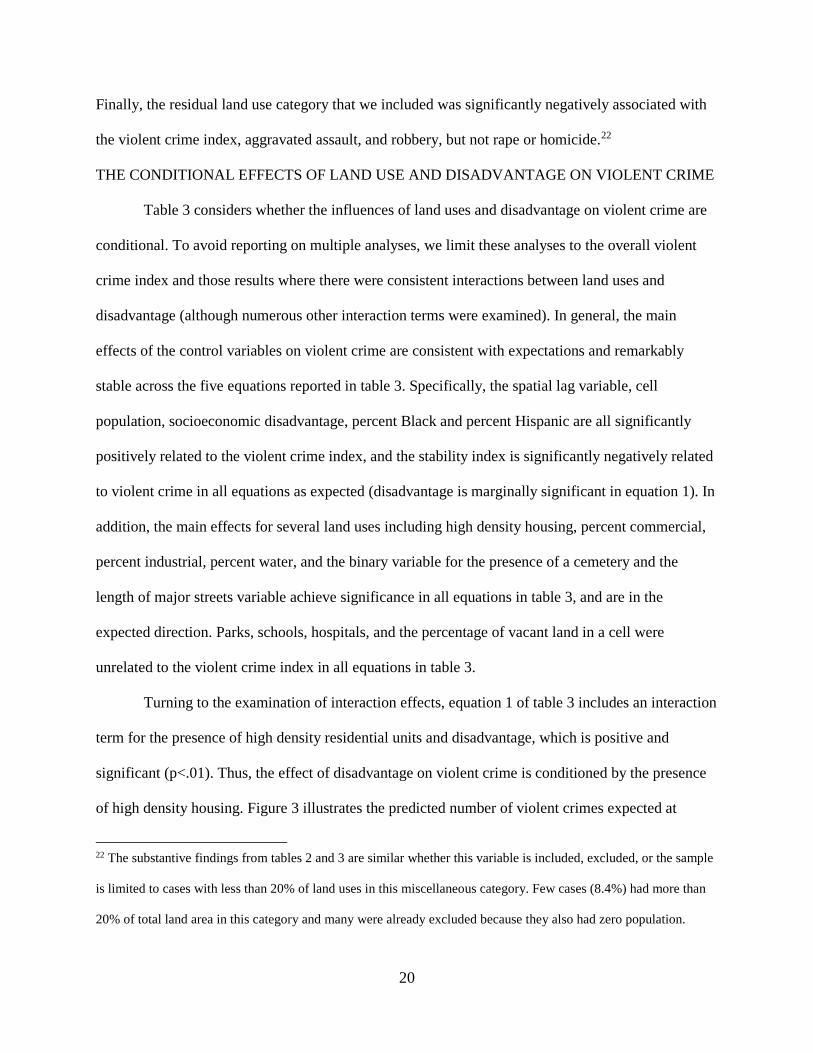
Turning to the examination of interaction effects, equation 1 of table 3 includes an interaction
term for the presence of high density residential units and disadvantage, which is positive and
significant (p<.01). Thus, the effect of disadvantage on violent crime is conditioned by the presence
of high density housing. Figure 3 illustrates the predicted number of violent crimes expected at
22 The substantive findings from tables 2 and 3 are similar whether this variable is included, excluded, or the sample
is limited to cases with less than 20% of land uses in this miscellaneous category. Few cases (8.4%) had more than
20% of total land area in this category and many were already excluded because they also had zero population.
20
various levels of the disadvantage index depending on the presence or absence of high density
residential units in the cell (assuming the cell contained no schools, cemeteries, or hospitals and other
variables were at their means). Even in highly advantaged areas (i.e., the left side of the figure), areas
with high density housing have somewhat higher expected numbers of violent crimes. However, as
the area becomes more disadvantaged, the effect of high density housing on violent crime becomes
more pronounced. Interestingly, predicted violent crime counts in highly advantaged cells with high
density housing are only slightly lower than predicted violent crime counts in extremely
disadvantaged areas with no high density housing. Thus, it appears that high density housing is
associated with higher violent crimes but especially so in disadvantaged areas.
Figure 3 about here
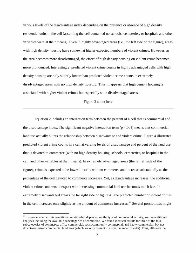
Equation 2 includes an interaction term between the percent of a cell that is commercial and
the disadvantage index. The significant negative interaction term (p <.001) means that commercial
land use actually blunts the relationship between disadvantage and violent crime. Figure 4 illustrates
predicted violent crime counts in a cell at varying levels of disadvantage and percent of the land use
that is devoted to commerce (with no high density housing, schools, cemeteries, or hospitals in the
cell, and other variables at their means). In extremely advantaged areas (the far left side of the
figure), crime is expected to be lowest in cells with no commerce and increase substantially as the
percentage of the cell devoted to commerce increases. Yet, as disadvantage increases, the additional
violent crimes one would expect with increasing commercial land use becomes much less. In
extremely disadvantaged areas (the far right side of figure 4), the predicted number of violent crimes
in the cell increases only slightly as the amount of commerce increases.23 Several possibilities might
23 To probe whether this conditional relationship depended on the type of commercial activity, we ran additional analyses including the available subcategories of commerce. We found identical results for three of the four subcategories of commerce: office commercial, retail/community commercial, and heavy commercial, but not downtown mixed commercial land uses (which are only present in a small number of cells). Thus, although the
21
explain this finding. First, it could be that commercial activities in advantaged areas bring relatively
larger numbers of motivated offenders than in disadvantaged areas where more of these offenders
might already be located. Or it could be that commercial activities in advantaged areas are associated
with much more attractive targets for offenders. Although we can only speculate without additional
data, the current results challenge the notion that commerce is invariably associated with higher
crime regardless of the socioeconomic context.
Figure 4 about here
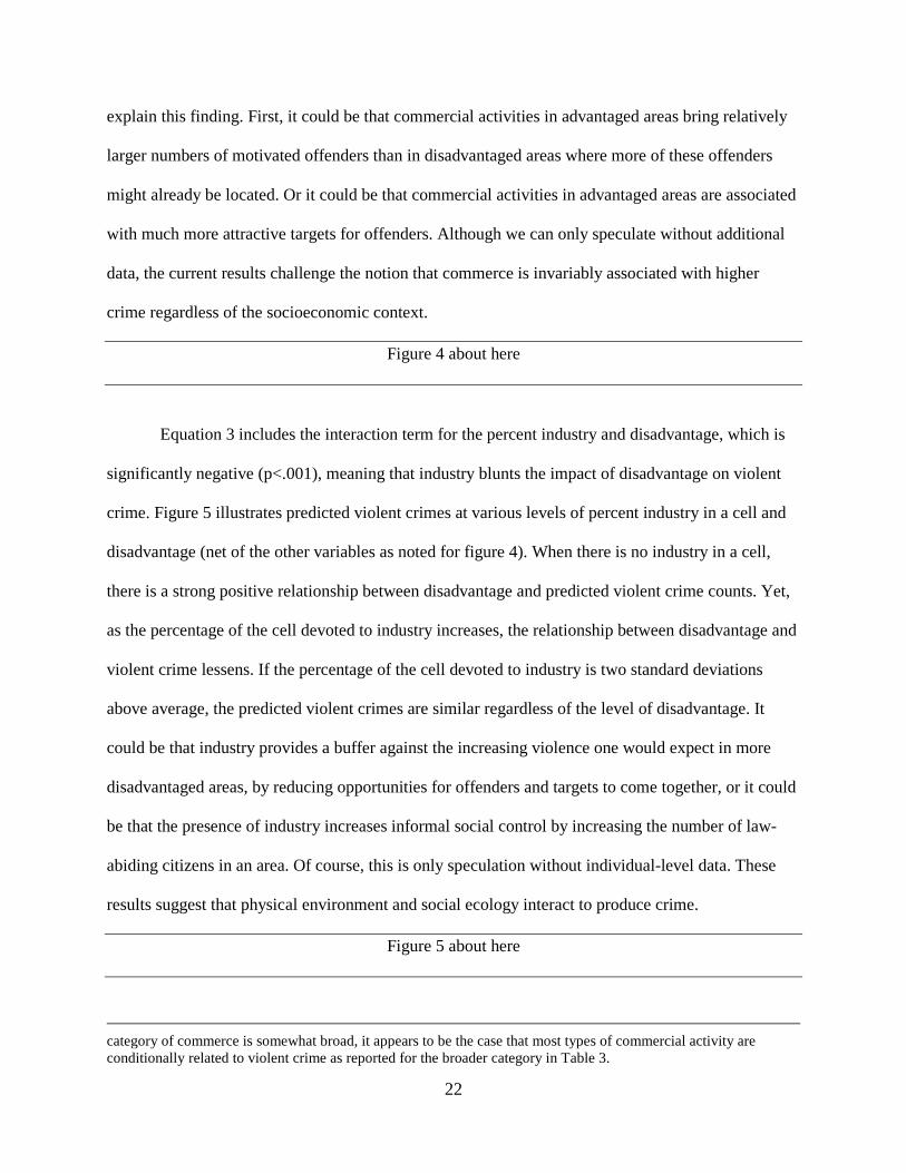
Equation 3 includes the interaction term for the percent industry and disadvantage, which is
significantly negative (p<.001), meaning that industry blunts the impact of disadvantage on violent
crime. Figure 5 illustrates predicted violent crimes at various levels of percent industry in a cell and
disadvantage (net of the other variables as noted for figure 4). When there is no industry in a cell,
there is a strong positive relationship between disadvantage and predicted violent crime counts. Yet,
as the percentage of the cell devoted to industry increases, the relationship between disadvantage and
violent crime lessens. If the percentage of the cell devoted to industry is two standard deviations
above average, the predicted violent crimes are similar regardless of the level of disadvantage. It
could be that industry provides a buffer against the increasing violence one would expect in more
disadvantaged areas, by reducing opportunities for offenders and targets to come together, or it could
be that the presence of industry increases informal social control by increasing the number of law-
abiding citizens in an area. Of course, this is only speculation without individual-level data. These
results suggest that physical environment and social ecology interact to produce crime.
Figure 5 about here
category of commerce is somewhat broad, it appears to be the case that most types of commercial activity are conditionally related to violent crime as reported for the broader category in Table 3.
22
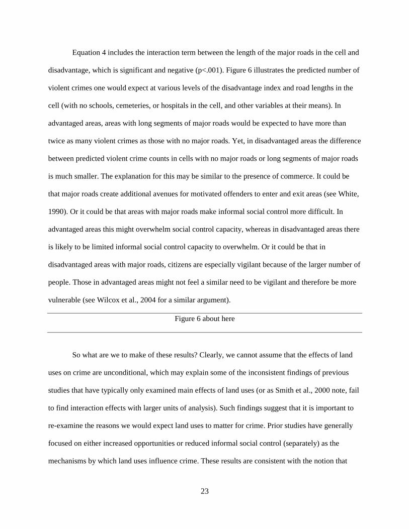
Equation 4 includes the interaction term between the length of the major roads in the cell and
disadvantage, which is significant and negative (p<.001). Figure 6 illustrates the predicted number of
violent crimes one would expect at various levels of the disadvantage index and road lengths in the
cell (with no schools, cemeteries, or hospitals in the cell, and other variables at their means). In
advantaged areas, areas with long segments of major roads would be expected to have more than
twice as many violent crimes as those with no major roads. Yet, in disadvantaged areas the difference
between predicted violent crime counts in cells with no major roads or long segments of major roads
is much smaller. The explanation for this may be similar to the presence of commerce. It could be
that major roads create additional avenues for motivated offenders to enter and exit areas (see White,
1990). Or it could be that areas with major roads make informal social control more difficult. In
advantaged areas this might overwhelm social control capacity, whereas in disadvantaged areas there
is likely to be limited informal social control capacity to overwhelm. Or it could be that in
disadvantaged areas with major roads, citizens are especially vigilant because of the larger number of
people. Those in advantaged areas might not feel a similar need to be vigilant and therefore be more
vulnerable (see Wilcox et al., 2004 for a similar argument).
Figure 6 about here
So what are we to make of these results? Clearly, we cannot assume that the effects of land
uses on crime are unconditional, which may explain some of the inconsistent findings of previous
studies that have typically only examined main effects of land uses (or as Smith et al., 2000 note, fail
to find interaction effects with larger units of analysis). Such findings suggest that it is important to
re-examine the reasons we would expect land uses to matter for crime. Prior studies have generally
focused on either increased opportunities or reduced informal social control (separately) as the
mechanisms by which land uses influence crime. These results are consistent with the notion that
23
opportunity and informal social control interact to produce variation in violent crime in urban areas.
Of course, we can only speculate on these issues without additional data that is beyond the scope of
the current study.
CHECKS FOR ROBUSTNESS
To examine the robustness of the findings reported in tables 2 and 3, we conducted a number
of additional analyses. First, equation 5 of Table 3 shows that the reported effects remain when all
interactions are included. Second, it is important to note that numerous additional interaction effects
were tested for land use and socioeconomic characteristic combinations (e.g., hospital, schools,
water, vacant land, and cell population by disadvantage interactions, as well as interactions with the
stability index), and none were consistently significant. We ran sensitivity analyses for the effects of
specific variables. For example, to explore whether the results were influenced by the inclusion of
cells with few residents, when models were restricted to cells with 20 or more residents or 50 or more
residents, substantively similar estimates were produced. We also ran models that employed mean
substitution to replace missing data and found only two differences from those reported in tables 2
and 3. In some models, parks became statistically significantly negatively associated with violent
crimes and the stability index declined to non-significance in some models. Otherwise substantive
conclusions were identical to those reported.
To investigate the potential that outliers might influence the significance of land uses, for the
1000-feet cell models we restricted the analyses to cells with less than 80 percent devoted to
industrial, water, or park uses, and found similar results. We observed no obvious outliers for any of
the dependent variables. We ran models limiting the sample to cells with less than 20 percent of
residual land uses and found similar results to those reported here.
We conducted analyses using 500 X 500 feet cells and these results showed that the effects of
specific land uses such as percent commercial and percent industrial interacted with the level of
disadvantage in an area to produce violent crime variation. Thus, substantively similar conclusions
24
about the direct and conditional impacts of land use and disadvantage were reached with smaller
units of analysis (and a much larger N).
We also conducted analyses which calculated socioeconomic variables with the 2000 census
area characteristics within a ½ mile radius of the cell rather than the cell itself. Again, substantively
similar results were produced regarding the direct and conditional effects of land uses and
disadvantage on violent crimes. Finally, we calculated a spatial lag variable of the disadvantage
index, and models which controlled for the average level of disadvantage in the 8 surrounding cells
(in a 3 X 3 grouping of cells) produced results substantively equivalent to those reported in table 3.
DISCUSSION AND CONCLUSIONS
Some prior research has suggested that land uses and crime are related, although studies have
tended to focus on specific land uses and generally investigated only main effects of land uses. The
current study moved beyond prior research by considering main and conditional effects of a variety
of land uses on several serious violent crimes. Using socioeconomic and land use information for
regular shaped 1000 X 1000 feet cells in the IPD service area we found that specific land uses are
related to a violent crime index of UCR reported crimes, and homicide, rape, robbery, and aggravated
assaults, net of the variables typically included in violent crime models. Specifically, we found that
commercial activity and high density residential land uses were associated with higher violent crime
counts, whereas cemeteries, water, and industry were associated with lower counts for some violent
crimes. Thus, it does not appear that all nonresidential land uses are associated with higher crime. In
addition, the influences of several land uses on violent crime counts were conditional on the
socioeconomic characteristics of the cell. Specifically, we found that the effects of busy roads, high
density residential units, commerce and industrial land uses on violent crime counts all depended on
the disadvantage index (and vice versa). Yet, high density residential units enhanced the impact of
disadvantage on violent crime, whereas commerce, industry, and busy roads dampened the effect of
disadvantage. Thus, both residential and nonresidential land uses can increase or decrease crime but
25
their effects depend on the socioeconomic context surrounding them.
In addition to confirming the importance of land uses for explaining violent crime, net of
socioeconomic variables, the current study has implications for both systemic social
disorganization/collective efficacy theories and routine activities/opportunity theories. As we noted
earlier, there has been exploration of land use-crime relationships at least since the early days of the
Chicago school. For example, Shaw and Mckay’s classic discussion of transition zones shows that
land uses are systematically related to social (dis)organization. They noted that the highest
delinquency areas were those that were in close proximity to industrial or commercial areas. Yet,
Shaw and Mckay (1972[1942]: 143) dismissed the notion that land uses caused delinquency:
There is, of course, little reason to postulate a direct relationship between living in proximity
to industrial developments and becoming delinquent. While railroads and industrial
properties may offer a field for delinquent behavior, they can hardly be regarded as a cause
for such activities.
Consistent with this, subsequent research and theorizing in systemic social disorganization
has primarily focused on social ecology rather than land uses and so, with few exceptions (Sampson
and Raudenbush1999, 2004; Smith et al. 2000; Taylor, 1997; Wilcox et al., 2004), mainstream
research on social disorganization/collective efficacy (Morenoff, Sampson, and Raudenbush, 2001;
Sampson and Groves, 1989; Sampson, Raudenbush, and Earls, 1997) has excluded land use
variables. Yet, the current study suggests that Shaw and Mckay may have been incorrect to presume
that land uses themselves would be unlikely to have independent effects on crime (see also
Brantingham and Jeffery, 1981). One of the key findings of the original Shaw and Mckay study was
that neighborhoods tended to have stable rates of delinquency despite changes in their racial and
ethnic composition over time. They interpreted this to mean that neighborhood social structural
characteristics created some enduring constraints on the ability of neighborhoods to generate
informal social control. It seems quite likely that they undersold the importance of how the enduring
26
physical characteristics of neighborhoods also structured social interactions in patterned ways that
created opportunities for delinquency—which is even suggested by the reference to industrial areas
as “offering a field for delinquent behavior” in the quote above. Given the relatively stable nature of
land use configurations in areas over time, it seems likely that some of the observed stability in
neighborhood delinquency rates was due to the enduring physical characteristics of the
neighborhoods. Of course, this speculation goes beyond the findings of the current cross-sectional
study but our results suggest that theorists explicitly need to bring physical structure back into social
disorganization/collective efficacy theories.
This study also suggests that the focus on the breakdown of social institutions in systemic
social disorganization theory may be overly narrow. In addition to being amorphous, difficult to
measure social constructs, social institutions such as religion, education, and the economy have
tangible physical manifestations that structure social interactions in patterned ways. Thus, the
importance of education or commerce may not only be in how it influences the capacity for informal
social control but also in how the physical land uses associated with such activities structure social
interaction and, as a result, opportunities for crime.
The current study also suggests that theories focusing on the breakdown of social institutions
only tell part of the story. Ecological theories such as social disorganization and institutional anomie
theories also need to focus on social institutions at work and the complex interplay of social
institutions that generate particular land use configurations. Students of urban politics are keenly
aware that zoning and resulting land use configurations are not natural phenomena. Therefore, the
placement of certain land uses is intimately tied to how neighborhoods can or fail to mobilize to say
“Not in My Back Yard” to some land uses perceived as undesirable. Or, conversely, how well
neighborhoods mobilize to create or maintain desirable neighborhoods through zoning or code
enforcement can have important effects on crime (see Bursik, 1989).
The findings of the current study also have implications for land use planners. For example, it
27
appears that busy roads and high density housing can produce additional violent crime but busy roads
have more of an impact in advantaged areas whereas high density housing has more of an impact in
disadvantaged areas. It also appears that industry may be a buffer against violence, especially in
disadvantaged areas.
This study also suggests new avenues of development for routine activities/opportunity
theories of crime. For example, land uses are mentioned in Sherman et al.’s (1989) seminal work on
“hot spots” (see also Kennedy and Forde, 1990). Such stability of crime hot spots was recently
confirmed in Weisburd et al.’s (2004) study of crime trajectories of street segments in Seattle. Yet,
such work is too often ad hoc. Hot spots, however, don’t simply appear at random, nor do they result
solely from the socioeconomic characteristics of the neighborhood. They are the result of how
particular land uses structure the routine activities of daily life and social interactions in patterned
ways. Therefore, small area research would benefit from additional consideration of how to
systematically include land use information and how such land uses structure social interactions and
opportunities for crime. Including land use information could help to make sense of how routine
activities and the corresponding opportunities for crime come together in a structured way to move
beyond the empirically-driven approaches often taken in such research.
The findings of the current study also provide additional evidence supporting the integration
of social disorganization and routine activities theories. For example, Smith et al. (2000) began to
empirically integrate routine activities and social disorganization theories in their study of robbery in
face blocks (see also Wilcox, Land, and Hunt, 2003; Wilcox, Quisenberry, and Jones, 2003, 2004).
Although such a study is a good beginning, more theoretical work is necessary to fully integrate
situational and ecological theories, which is likely the best way to capitalize on the strengths of both.
Despite the contributions of the current study, some limitations should be noted. One
weakness of the current study is the inability to distinguish within certain categories of land uses. For
example, the current data could not distinguish liquor establishments from other kinds of commercial
28
businesses or elementary schools from high schools. Future research needs to examine more closely
the extent to which different kinds of commercial activity increase violent crime more than others. A
second limitation of this study is that we did not have access to data on property crimes. We did,
however, find fairly consistent effects of land uses across violent crimes. Future research should
consider whether the effects of land uses found in the current study also apply for property crimes
such as burglary and theft. A third limitation of this study is that it is cross-sectional. Given the
stability of land use configurations, it seems unlikely that crime is driving land uses (at least in the
short-term). Yet, future research should examine long term dynamic models of land use and crime.
We were also unable to measure informal social control, incivilities, or opportunity directly in the
current study. Therefore, our study cannot address such issues. Fully explicating the role of land uses
in generating violent crime awaits a study that can incorporate measurements of these key
intervening variables. Finally, our study only includes land use information from one city. Although
there is little reason to believe that the kinds of land uses examined here would have different effects
in other cities, and the data analyzed here come from a fairly typical older large Midwest city, such
comparisons with other cities in future research would help clarify the generality of the findings of
the current study.
In sum, we find that specific land uses affect violent crime, and the effects of such land uses
on violent crime vary depending on the socioeconomic disadvantage in the area. We believe that
such results suggest important revisions to existing ecological and situational theories are necessary
to incorporate land uses into theoretical models. Land uses also may provide a way to integrate
ecological and situational models to develop a fuller explanation of crime.
29
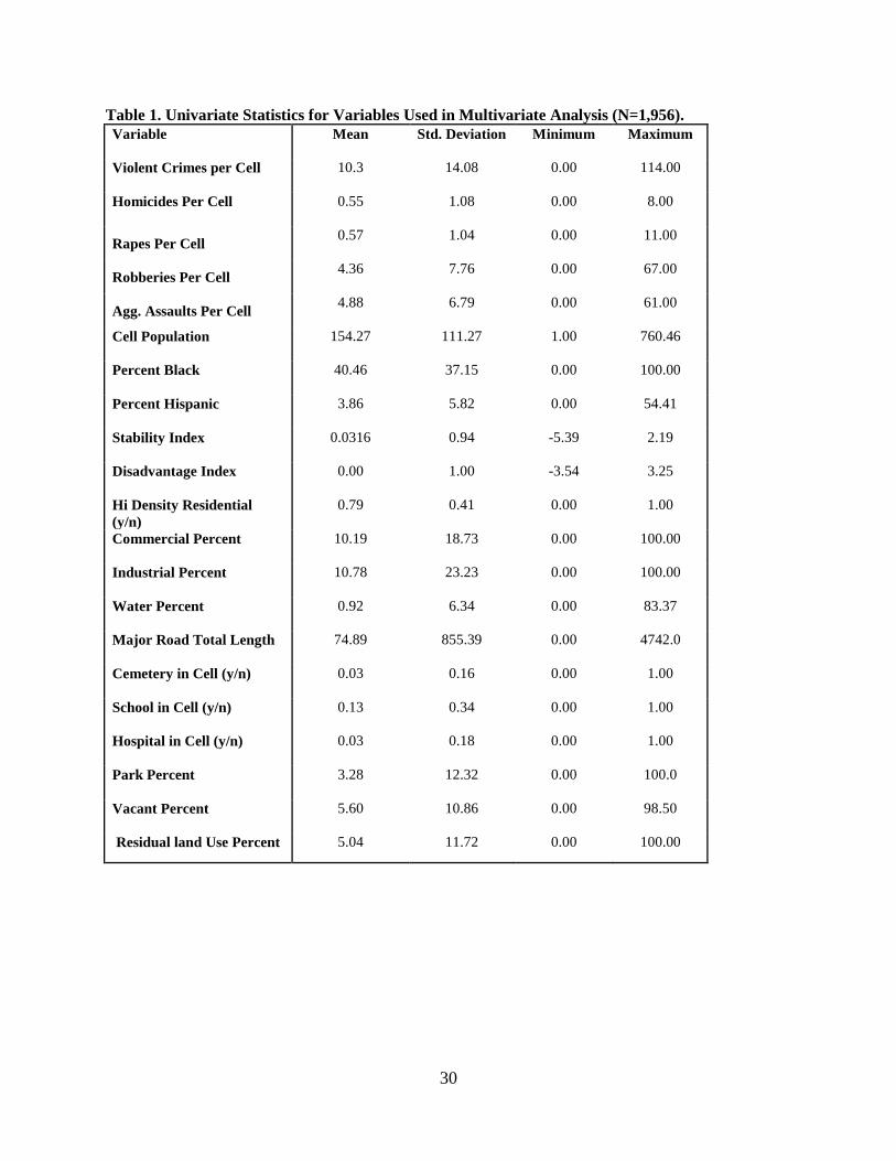
Table 1. Univariate Statistics for Variables Used in Multivariate Analysis (N=1,956). Variable
Mean
Std. Deviation
Minimum
Maximum
Violent Crimes per Cell
10.3
14.08
0.00
114.00
Homicides Per Cell
0.55
1.08
0.00
8.00
Rapes Per Cell 0.57
1.04
0.00
11.00
Robberies Per Cell 4.36
7.76
0.00
67.00
Agg. Assaults Per Cell 4.88
6.79
0.00
61.00
Cell Population
154.27
111.27
1.00
760.46
Percent Black
40.46
37.15
0.00
100.00
Percent Hispanic
3.86
5.82
0.00
54.41
Stability Index
0.0316
0.94
-5.39
2.19
Disadvantage Index
0.00
1.00
-3.54
3.25
Hi Density Residential (y/n)
0.79
0.41
0.00
1.00
Commercial Percent
10.19
18.73
0.00
100.00
Industrial Percent
10.78
23.23
0.00
100.00
Water Percent
0.92
6.34
0.00
83.37
Major Road Total Length
74.89
855.39
0.00
4742.0
Cemetery in Cell (y/n)
0.03
0.16
0.00
1.00
School in Cell (y/n)
0.13
0.34
0.00
1.00
Hospital in Cell (y/n)
0.03
0.18
0.00
1.00
Park Percent
3.28
12.32
0.00
100.0
Vacant Percent
5.60
10.86
0.00
98.50
Residual land Use Percent 5.04 11.72 0.00 100.00
30
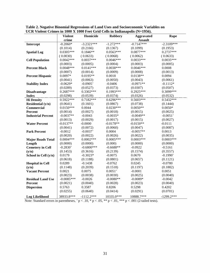
Table 2. Negative Binomial Regressions of Land Uses and Socioeconomic Variables on UCR Violent Crimes in 1000 X 1000 Feet Grid Cells in Indianapolis (N=1956).
Violent crime
Homicide
Robbery
Aggravated Assault
Rape
Intercept
-0.2060* (0.1014)
-3.2321*** (0.2166)
-1.272*** (0.1367)
-0.7147*** (0.1099)
-2.3109*** (0.1953)
Spatial Lag
0.0305*** ( 0.0030)
0.1846** ( 0.0633)
0.0563*** ( 0.0068)
0.0877*** ( 0.0062)
0.2737*** ( 0.0633)
Cell Population
0.0042*** (0.0003)
0.0037*** (0.0005)
0.0046*** (0.0004)
0.0033*** (0.0003)
0.0035*** (0.0005)
Percent Black
0.0048*** (0.0007)
0.0141*** (0.0014)
0.0038*** (0.0009)
0.0046*** (0.0008)
0.0008 (0.0013)
Percent Hispanic
0.0097* (0.0041)
0.0195** (0.0063)
0.0018 (0.0050)
0.0138** (0.0043)
0.0094 (0.0061)
Stability Index
-0.0629* (0.0289)
-0.0905+ (0.0527)
-0.0406 (0.0373)
-0.0971** (0.0307)
-0.1112* (0.0507)
Disadvantage Index
0.2687*** (0.0298)
0.3302*** (0.0539)
0.1993*** (0.0374)
0.2925*** (0.0326)
0.3099*** (0.0532)
Hi Density Residential (y/n)
0.5922*** (0.0641)
0.7182*** (0.1601)
0.6296*** (0.0867)
0.5603*** (0.0738)
0.5432*** (0.1444)
Commercial Percent
0.0150*** (0.0014)
0.0044 (0.0027)
0.0230*** (0.0018)
0.0050** (0.0015)
0.0050* (0.0025)
Industrial Percent
-0.0037** (0.0013)
-0.0043 (0.0029)
-0.0035* (0.0017)
-0.0049** (0.0015)
-0.0051+ (0.0027)
Water Percent
-0.0137** (0.0041)
-0.0000 (0.0072)
-0.0178** (0.0060)
-0.0150** (0.0047)
-0.0111 (0.0087)
Park Percent
-0.0012 (0.0020)
-0.0037+ (0.0022)
0.0004 (0.0026)
-0.0057** (0.0022)
0.0013 (0.0035)
Major Roads Total Length
0.0004*** (0.0000)
0.0002*** (0.0000)
0.0005*** (0.000)
0.0003*** (0.0000)
0.0003*** (0.0000)
Cemetery in Cell (y/n)
-0.2830+ (0.1453)
-0.6800*** (0.3616)
-0.6688** (0.2139)
-0.0922 (0.1574)
-0.5161 (0.3557)
School in Cell (y/n)
0.0179 (0.0618)
-0.3023* (0.1188)
-0.0075 (0.0801)
0.0670 (0.0657)
-0.1990+ (0.1121)
Hospital in Cell (y/n)
0.0289 (0.1148)
-0.1438 (0.2039)
-0.0762 (0.1518)
0.0245 (0.1197)
-0.0780 (0.1882)
Vacant Percent
0.0021 (0.0023)
0.0075 (0.0038)
0.0051+ (0.0030)
-0.0001 (0.0025)
0.0051 (0.0040)
Residual Land Use Percent
-0.0085*** (0.0021)
-0.0026 (0.0040)
-0.0080** (0.0028)
-0.0089* (0.0023)
-0.0042 (0.0040)
Dispersion
0.5763 (0.0255)
0.3587 (0.0640)
0.8206 (0.0414)
0.5298 (0.0291)
0.4202 (0.0701)
Log Likelihood 38933.8*** -1112.2*** 10335.0*** 10888.7*** -1299.2*** Note: Standard errors in parentheses, + p < .10, * p < .05, ** p < .01, *** p < .001 (2-tailed tests).
31
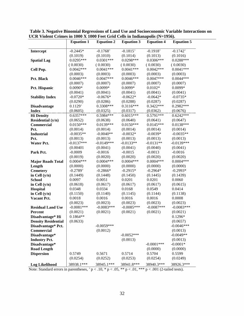
Table 3. Negative Binomial Regressions of Land Use and Socioeconomic Variable Interactions on UCR Violent Crimes in 1000 X 1000 Feet Grid Cells in Indianapolis (N=1956).
Equation 1
Equation 2
Equation 3
Equation 4
Equation 5
Intercept
-0.2445* (0.1019)
-0.1768+ (0.1010)
-0.1815+ (0.1014)
-0.1918+ (0.1013)
-0.1742+ (0.1016)
Spatial Lag
0.0295*** ( 0.0030)
0.0301*** ( 0.0030)
0.0298*** ( 0.0030)
0.0306*** ( 0.0030)
0.0288*** ( 0.0030)
Cell Pop.
0.0042*** (0.0003)
0.0041*** (0.0003)
0.0041*** (0.0003)
0.0042*** (0.0003)
0.0041*** (0.0003)
Pct. Black
0.0046*** (0.0007)
0.0047*** (0.0007)
0.0046*** (0.0007)
0.0047*** (0.0007)
0.0044*** (0.0007)
Pct. Hispanic
0.0090* (0.0041)
0.0099* (0.0041)
0.0099* (0.0041)
0.0102* (0.0041)
0.0099* (0.0041)
Stability Index
-0.0720* (0.0290)
-0.0676* (0.0286)
-0.0622* (0.0288)
-0.0642* (0.0287)
-0.0735* (0.0287)
Disadvantage Index
0.1129+ (0.0605)
0.3308*** (0.0325)
0.3116*** (0.0317)
0.3422*** (0.0362)
0.2982*** (0.0676)
Hi Density Residential (y/n)
0.6357*** (0.0652)
0.5984*** (0.0638)
0.6015*** (0.0640)
0.5791*** (0.0641)
0.6242*** (0.0647)
Commercial Pct.
0.0150*** (0.0014)
0.0139*** (0.0014)
0.0150*** (0.0014)
0.0145*** (0.0014)
0.0138*** (0.0014)
Industrial Pct.
-0.0035** (0.0013)
-0.0040** (0.0013)
-0.0032* (0.0013)
-0.0039* (0.0013)
-0.0035** (0.0013)
Water Pct.
-0.0137*** (0.00401
-0.0149*** (0.0041)
-0.0133** (0.0041)
-0.0131** (0.0040)
-0.0139*** (0.0041)
Park Pct.
-0.0009 (0.0019)
-0.0016 (0.0020)
-0.0015 (0.0020)
-0.0013 (0.0020)
-0.0016 (0.0020)
Major Roads Total Length
0.0004*** (0.0000)
0.0004*** (0.0000)
0.0004*** (0.0000)
0.0004*** (0.0000)
0.0004*** (0.0000)
Cemetery in Cell (y/n)
-0.2789+ (0.1449)
-0.2866* (0.1448)
-0.2915* (0.1450)
-0.2964* (0.1445)
-0.2993* (0.1439)
School in Cell (y/n)
0.0097 (0.0618)
0.0051 (0.0617)
0.0201 (0.0617)
0.0201 (0.0617)
0.0060 (0.0615)
Hospital in Cell (y/n)
0.0348 (0.1150)
0.0334 (0.1140)
0.0168 (0.1145)
0.0549 (0.1144)
0.0414 (0.1138)
Vacant Pct.
0.0018 (0.0023)
0.0016 (0.0023)
0.0016 (0.0023)
0.0016 (0.0023)
0.0008 (0.0023)
Residual Land Use Percent
-0.0081*** (0.0021)
-0.0083*** (0.0021)
-0.0085*** (0.0021)
-0.0087*** (0.0021)
-0.0083*** (0.0021)
Disadvantage* Hi Density Residential
0.1864** (0.0633)
0.1296* (0.0657)
Disadvantage* Pct. Commercial
-0.0059*** (0.0012)
-0.0046*** (0.0013)
Disadvantage* Industry Pct.
-0.0052*** (0.0013)
-0.0049** (0.0013)
Disadvantage* Road Length
-0.0001*** (0.0000)
-0.0001* (0.0000)
Dispersion
0.5749 (0.0254)
0.5671 (0.0252)
0.5714 (0.0253)
0.5704 (0.0254)
0.5599 (0.0249)
Log Likelihood 38938.1*** 38945.1*** 38941.8*** 38940.3*** 38926.3*** Note: Standard errors in parentheses, + p < .10, * p < .05, ** p < .01, *** p < .001 (2-tailed tests).
32
References
Brantingham, Paul J. and Patricia L. Brantingham (eds.)1981. Environmental Criminology. Beverly
Hills, CA: Sage Publications.
Brantingham, Paul J. and C. Ray Jeffery. 1981. Afterword: Crime, space, and criminological theory.
In Environmental Criminology, eds. Paul J. Brantingham and Patricia L. Brantingham. Beverly Hills,
CA: Sage Publications.
Brunson, Liesette, Frances E. Kuo, and William C. Sullivan. 2001. Resident appropriation of
defensible space in public housing. Environment and Behavior 33:626-652.
Bursik, Robert J. 1989. Political decision-making and ecological models of delinquency: Conflict and
consensus. In Theoretical Integration in the Study of Deviance and Crime, eds. Steven F. Messner,
Marvin D. Krohn, and Allen E. Liska. Albany: State University of New York Press.
Bursik, Robert J. 1988. Social disorganization and theories of crime and delinquency: Problems and
prospects. Criminology 26: 519-551.
Burgess, E. W. 1916. Juvenile delinquency in a small city. Journal of the American Institute of
Criminal Law and Criminology 6:724-728.
Cahill, Meagan Elizabeth. 2005. Geographies of Urban Crime: An Intraurban Study of Crime in
Nashville, TN; Portland, OR; and Tucson, AZ. Unpublished Dissertation Thesis available at
http://www.ncjrs.gov/pdffiles1/nij/grants/209263.pdf.
33
Duffala, Dennis C. 1976. Convenience stores, armed robbery, and physical environmental features.
American Behavioral Scientist 20:227-246.
Eck, John E. 2002. Preventing crime at places. In Evidence-based Crime Prevention, eds. Lawrence
W. Sherman, David P. Farrington, Brandon C. Welsh, and Doris Layton Mackenzie. New York, NY:
Routledge.
Felson, Marcus. 1987. Routine activities and crime prevention in the developing metropolis.
Criminology 25:911-931.
Felson, Marcus. 2002. Crime and Everyday Life. Third edition. Thousand Oaks, CA: Sage
Publications.
Fotheringham, A. Stewart, Chris Brunsdon, and Martin Charlton. 2000. Quantitative Geography:
Perspectives on Spatial Data Analysis. London: Sage Publications.
Fowler, E. P. 1987. Street management and city design. Social Forces 66:365-389.
Gardiner, Richard A. 1978. Design for Safe Neighborhoods. Washington, D.C.: National Institute of
Law Enforcement and Criminal Law Enforcement Assistance Administration.
Greenberg, Stephanie W. and William M. Rohe. 1984. Neighborhood design and crime: A test of two
perspectives. American Planning Association Journal 50:48-61.
34
Greenberg, Stephanie W., William M. Rohe, and Jay R. Williams. 1982. Safe and Secure
Neighborhoods: Physical Characteristics and Informal Territorial Control in High and Low Crime
Neighborhoods. USGPO: National Institute of Justice
Greene, William H. 2000. Econometric Analysis, 4th edition. Upper Saddle River, NJ: Prentice Hall.
Jacobs, Jane. 1961. The Death and Life of Great American Cities. New York City, NY: Random
House.
Jeffery, C. Ray. 1976. Criminal behavior and the physical environment. American Behavioral
Scientist 20:149-174.
Jeffery C. Ray. 1977. Crime Prevention through Environmental Design. Beverly Hills, CA: Sage
Publications.
Kennedy, Leslie W. and David R. Forde. 1990. Routine activities and crime: An analysis of
victimization in Canada. Criminology 28:137-152.
Kurtz, Ellen M., Barbara A. Koons, and Ralph B. Taylor. 1998. Land use, physical deterioration,
resident-based control, and calls for service on urban street blocks. Justice Quarterly 15:121-149.
Lab, Steven, P. 1992. Crime Prevention: Approaches, Practices, and Evaluations. Second edition.
Cincinnati, OH: Anderson Publishing Company.
35
LaGrange, Teresa C. 1999. The impact of neighborhoods, schools, and malls on the spatial
distribution of property damage. Journal of Research in Crime and Delinquency 36:393-422.
Land, Kenneth C., Patricia L. McCall, and Lawrence E. Cohen. 1990. Structural covariates of
homicide rates: Are there any invariances across time and social space? American Journal of
Sociology 95:922-963.
Ley, David, and Roman Cybriwsky. 1974. The spatial ecology of stripped cars. Environment and
Behavior 6:53-68.
Lockwood, Daniel. 2007. Mapping crime in Savannah: Social disadvantage, land use, and violent
crimes reported to the police. Social Science Computer Review 25:194-209.
Loukaitou-Sideris, Anastasia. 1999. Hot spots of bus stop crime: The importance of environmental
attributes. American Planning Association Journal 65:395-411.
Mawby, R. I. 1976. Defensible space: A theoretical and empirical appraisal. Urban Studies.14:169-
179.
McCord, Eric S., Jerry H. Ratcliffe, R. Marie Garcia and Ralph B. Taylor. 2007. Nonresidential
attractors and generators elevate perceived neighborhood crime and incivilities. Journal of Research
in Crime and Delinquency 44:295-320.
Merry, Sally E. 1981. Defensible space undefended: Social factors in crime control through
environmental design. Urban Affairs Quarterly 16:397-422.
36
McNulty, Thomas L. and Steven R. Holloway. 2000. Race, crime and public housing in Atlanta:
Testing a conditional effect hypothesis. Social Forces 79:707-729.
Moran, Patrick A.P. 1948. The interpretation on statistical maps. Journal of the Royal Statistical
Society B 10: 243-251.
Morenoff, Jeffrey D., Robert J. Sampson and Steven W. Raudenbush. 2001. Neighborhood
inequality, collective efficacy, and the spatial dynamics of urban violence. Criminology 39:517-559.
Murray, Charles. 1983. The physical environment and community control of crime. In Crime
Prevention, ed. James Q. Wilson.. San Francisco, CA: Institute for Contemporary Studies Press.
Newman, Oscar. 1971. Architectural Design for Crime Prevention. Washington, D.C.: Law
Enforcement Assistance Administration, National Institute of Law Enforcement and Criminal
Justice.
Newman, Oscar. 1972. Defensible Space. New York City, NY: Macmillan Company.
Osgood, D. Wayne. 2000. Poisson-based regression analysis of aggregate crime rates. Journal of
Quantitative Criminology 16:21-43.
Osgood, D. Wayne, and Jeff M. Chambers. 2000. Social disorganization outside the metropolis: An
analysis of rural youth violence. Criminology 38: 81-115.
37
Parker, Karen F. and Patricia L. McCall. 1999. Structural conditions and racial homicide patterns: A
look at the multiple disadvantages in urban areas. Criminology 37:447-477.
Plaster-Carter, Sherry, Stanley L. Carter and Andrew L. Dannenberg. 2003. Zoning out crime and
improving community health in Sarasota, Florida: Crime prevention through environmental design.
American Journal of Public Health 93:1442-1445.
Roncek, Dennis W. and Antoinette Lobosco. 1983. The effect of high schools on crime in their
neighborhoods. Social Science Quarterly 64:599-613.
Roncek, Dennis W. and Donald Faggiani. 1985. High schools and crime: A replication. The
Sociological Quarterly 26:491-505.
Roncek, Dennis W. and Pamela Maier. 1991. Bars blocks and crimes revisited: Linking the theory of
routine activities to the empiricism of ‘hot spots.’ Criminology 29:725-753.
Roncek, Dennis W. and Mitchell A. Pravatiner. 1989. Additional evidence that taverns enhance
nearby crime. Sociology and Social Research 73:185-188.
Sampson, Robert J. and W. Byron Groves. 1989. Community structure and crime: Testing social
disorganization theory. American Journal of Sociology 94: 774-802.
Sampson, Robert J. and Stephen W. Raudenbush. 1999. Systemic social observation of public
spaces: A new look at disorder in urban neighborhoods. American Journal of Sociology 105:603-651.
38
Sampson, Robert J. and Stephen W. Raudenbush. 2004. Seeing disorder: Neighborhood stigma and
the social construction of ‘broken windows.’ Social Psychology Quarterly 67:319-342.
Sampson, Robert J., Stephen W. Raudenbush, and Felton Earls. 1997. Neighborhoods and violent
crime: A multilevel study of collective efficacy. Science 277:918-924.
Shaw, Clifford R. and Henry D. McKay. 1972[1942]. Juvenile Delinquency and Urban Areas.
Revised ed. Chicago, IL: The University of Chicago Press.
Sherman, Lawrence W., Patrick R. Gartin and Michael E. Buerger. 1989. Hot spots of predatory
crime: Routine activities and the criminology of place. Criminology 27:27-55.
Smith, William R., Sharon Glave Frazee, and Elizabeth L. Davison. 2000. Furthering the integration
of routine activity and social disorganization theories: Small units of analysis and the study of street
robbery as a diffusion process. Criminology 38:489- 523.
Taylor, Ralph B. 1997. Social order and disorder of street blocks and neighborhoods: Ecology,
microecology, and the systemic model of social disorganization. Journal of Research in Crime and
Delinquency 34:113-155.
Taylor, Ralph B. 1998. Crime and small-scale places: What we know, what we can prevent, and what
else we need to know. In Crime and Place: Plenary Papers of the 1997 Conference on Criminal
Justice Research and Evaluation, NCJ 168618, eds. Ralph B. Taylor, Gordon Bazemore, Barbara
Boland, Todd R. Clear, Ronald P. Corbett Jr., John Feinblatt, Greg Berman, Michelle Sviridoff and
Christopher Stone. Rockville, MD: National Institute of Justice.
39
Taylor, Ralph B., Stephen D. Gottfredson and Sidney Brower. 1980. The defensibility of defensible
space: A critical review and a synthetic framework for future research. In Understanding Crime, eds.
Travis Hirschi and Michael R. Gottfredson. Beverly Hills, CA: Sage Publications.
Taylor, Ralph B., Stephen D. Gottfredson, and Sidney Brower. 1984. Block crime and fear:
Defensible space, local social ties, and territorial functioning. Journal of Research in Crime and
Delinquency 21:303-331.
Taylor, Ralph B. and Stephen D. Gottfredson. 1986. Environmental design, crime, and prevention:
An examination of community dynamics. In Communities and Crime, eds. Albert J. Reiss, Jr. and
Michael Tonry. Chicago, IL: The University of Chicago Press.
Taylor, Ralph B., Barbara A. Koons, Ellen M. Kurtz, Jack R. Greene, and Douglas D. Perkins. 1995.
Street blocks with more nonresidential land use have more physical deterioration: Evidence from
Baltimore and Philadelphia. Urban Affairs Review 31:20-136.
Taylor, Ralph B. and Adele V. Harrell. 1996. Physical environment and crime. National Institute of
Justice Research Report, NCJ 157311. Rockville, MD: National Institute of Justice.
Wang, Fahui. 2007. Job access in disadvantaged neighborhoods in Cleveland, 1980-2000:
Implications for spatial mismatch and association with crime patterns. Cityscape: A Journal of Policy
Development and Research 9:95-121.
40
Weisburd, David, Shawn Bushway, Cynthia Lum and Sue-Ming Yang. 2004. Trajectories of crime at
places: A longitudinal study of street segments in the city of Seattle. Criminology 42:283-321.
White, Garland. 1990. Neighborhood permeability and burglary rates. Justice Quarterly 7:57-68.
White, R. Clyde. 1932. The relation of felonies to environmental factors in Indianapolis. Social
Forces 10:498-509.
Wilcox, Pamela, Kenneth C. Land, and Scott A. Hunt. 2003. Criminal Circumstance: A Dynamic
Multicontextual Criminal Opportunity Theory. New York: Aldine De Gruyter.
Wilcox, Pamela, Neil Quisenberry, and Shayne Jones. 2003. The built environment and community
crime risk interpretation. Journal of Research in Crime and Delinquency 40: 322-345.
Wilcox, Pamela, Neil Quisenberry, Debra T. Cabrera, and Shayne Jones. 2004. Busy places and
broken windows? Toward refining the role of physical structure and process in community crime
models. The Sociological Quarterly 45:185-207.
41
APPENDIX 1. DISCUSSION OF GRID CELLS AS THE UNITS OF ANLAYSIS
We chose 1000-feet grid cells as the units of analysis because other units of analysis
presented a variety of problems. An obvious choice for this type of spatial analysis would be census
subdivisions, either census tracts or block groups, which are familiar and widely used. We felt that
these were inappropriate for the current study for several reasons. First, these units are relatively
large and would have very significant heterogeneity in terms of land uses, reducing the ability to
distinguish the relationship between land use and crime. Second, because these units are defined to
have (very roughly) equal populations, they vary significantly in terms of land area, further
confounding the analysis of the spatial relationship between crime and land use. A final issue arises
from the fact that the boundaries of these units are generally streets. The UCR data have all been
geocoded to street centerlines. The geocoded locations are not offset to the side of the street on which
the address is located. This is reasonable because incidents can literally occur in the middle of the
street, with the address being used to identify location on the street as opposed to a parcel on either
side of the street. For crimes occurring on streets that form the boundaries of these units, ambiguity
would exist as to which tract or block group the crimes should be assigned.
Because census tracts and block groups are so widely employed in spatial analysis, there is a
tendency to assume that these are somehow “natural” units. Such an assumption seems potentially
problematic. Census tracts have been defined locally to be somewhat homogeneous areas. However,
this is limited by the constraints of establishing census tracts with roughly comparable populations
meeting the census criteria and tracts were often delineated decades ago. Such tracts may have been
relatively homogeneous when created but less so now, given population changes over time. For block
groups, no claim is made that these subdivisions reflect natural areas. They are defined for
administrative convenience by the Census Bureau.
Using census blocks would provide areas more appropriate for reducing the heterogeneity of
land use. However, the use of these units is highly problematic given IPD’s assignment of the crimes
42
to the street centerlines. Nearly all of the crimes would be assigned to the boundaries between the
census blocks, creating difficulties in consistently assigning the crimes to census blocks.
Perhaps the most reasonable “natural” units for analysis, suggested by one reviewer, would
be face blocks, single street segments of blocks. For areas with regular, rectangular blocks, these are
relatively well-defined units. However, in areas with irregular street patterns, the definition of the
face blocks becomes more ambiguous. Because of the structure of the UCR crime data provided by
IPD, many crimes have been geocoded to street intersections. This raises the ambiguity of assigning
those crimes to the (typically four) face block street segments at the intersection. Our use of grid cells
largely solves the problem of assigning the geocoded crimes to the correct unit. Though it is possible
that a grid cell boundary could intersect with a crime location, the probability of an exact intersection
is extremely small.
The major argument for using the grid cells as opposed to census tracts or block groups is to
reduce the heterogeneity of land use within the units of analysis (Map 3 shows a comparison of block
groups with the grid cells for Marion County). This cannot, of course, address potential issues in the
heterogeneity of socioeconomic characteristics within the units of analysis for which the census
reports those characteristics. Socioeconomic characteristics are necessarily derived from the census
data and are estimated for the grid cells by making the assumption that the characteristics are uniform
within the census units. However, for those characteristics available from the full-count, census block
data, block data were used to estimate grid cell values. The assumption is made only of homogeneity
within the small areas of the blocks, not the larger block group areas. For those characteristics from
the sample data, reported at the block group level as the smallest unit (foreign born, lived in same
residence, unemployment, poverty, and household income), the assumption is necessarily being made
of homogeneity within the block groups for estimation for the grid cells.
Map 3 about here
43
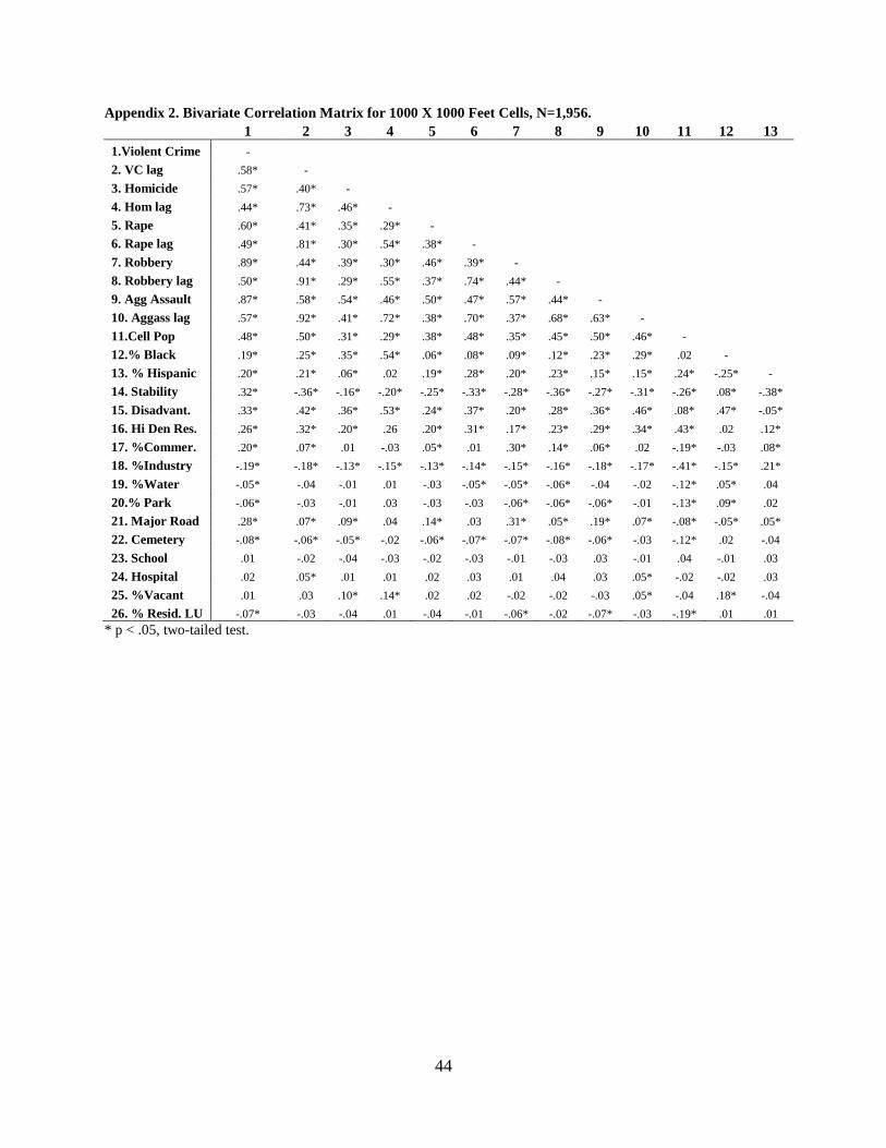
Appendix 2. Bivariate Correlation Matrix for 1000 X 1000 Feet Cells, N=1,956. 1 2 3 4 5 6 7 8 9 10 11 12 13 1.Violent Crime - 2. VC lag .58* - 3. Homicide .57* .40* - 4. Hom lag .44* .73* .46* - 5. Rape .60* .41* .35* .29* - 6. Rape lag .49* .81* .30* .54* .38* - 7. Robbery .89* .44* .39* .30* .46* .39* - 8. Robbery lag .50* .91* .29* .55* .37* .74* .44* - 9. Agg Assault .87* .58* .54* .46* .50* .47* .57* .44* - 10. Aggass lag .57* .92* .41* .72* .38* .70* .37* .68* .63* - 11.Cell Pop .48* .50* .31* .29* .38* .48* .35* .45* .50* .46* - 12.% Black .19* .25* .35* .54* .06* .08* .09* .12* .23* .29* .02 - 13. % Hispanic .20* .21* .06* .02 .19* .28* .20* .23* .15* .15* .24* -.25* - 14. Stability .32* -.36* -.16* -.20* -.25* -.33* -.28* -.36* -.27* -.31* -.26* .08* -.38* 15. Disadvant. .33* .42* .36* .53* .24* .37* .20* .28* .36* .46* .08* .47* -.05* 16. Hi Den Res. .26* .32* .20* .26 .20* .31* .17* .23* .29* .34* .43* .02 .12* 17. %Commer. .20* .07* .01 -.03 .05* .01 .30* .14* .06* .02 -.19* -.03 .08* 18. %Industry -.19* -.18* -.13* -.15* -.13* -.14* -.15* -.16* -.18* -.17* -.41* -.15* .21* 19. %Water -.05* -.04 -.01 .01 -.03 -.05* -.05* -.06* -.04 -.02 -.12* .05* .04 20.% Park -.06* -.03 -.01 .03 -.03 -.03 -.06* -.06* -.06* -.01 -.13* .09* .02 21. Major Road .28* .07* .09* .04 .14* .03 .31* .05* .19* .07* -.08* -.05* .05* 22. Cemetery -.08* -.06* -.05* -.02 -.06* -.07* -.07* -.08* -.06* -.03 -.12* .02 -.04 23. School .01 -.02 -.04 -.03 -.02 -.03 -.01 -.03 .03 -.01 .04 -.01 .03 24. Hospital .02 .05* .01 .01 .02 .03 .01 .04 .03 .05* -.02 -.02 .03 25. %Vacant .01 .03 .10* .14* .02 .02 -.02 -.02 -.03 .05* -.04 .18* -.04 26. % Resid. LU -.07* -.03 -.04 .01 -.04 -.01 -.06* -.02 -.07* -.03 -.19* .01 .01
* p < .05, two-tailed test.
44
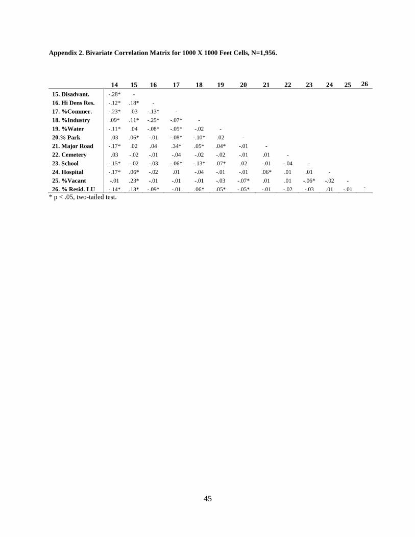
Appendix 2. Bivariate Correlation Matrix for 1000 X 1000 Feet Cells, N=1,956.
14 15 16 17 18 19 20 21 22 23 24 25 26 15. Disadvant. -.28* -
16. Hi Dens Res. -.12* .18* -
17. %Commer. -.23* .03 -.13* -
18. %Industry .09* .11* -.25* -.07* -
19. %Water -.11* .04 -.08* -.05* -.02 -
20.% Park .03 .06* -.01 -.08* -.10* .02 -
21. Major Road -.17* .02 .04 .34* .05* .04* -.01 -
22. Cemetery .03 -.02 -.01 -.04 -.02 -.02 -.01 .01 -
23. School -.15* -.02 -.03 -.06* -.13* .07* .02 -.01 -.04 -
24. Hospital -.17* .06* -.02 .01 -.04 -.01 -.01 .06* .01 .01 -
25. %Vacant -.01 .23* -.01 -.01 -.01 -.03 -.07* .01 .01 -.06* -.02 -
26. % Resid. LU -.14* .13* -.09* -.01 .06* .05* -.05* -.01 -.02 -.03 .01 -.01 -
* p < .05, two-tailed test.
45

Map 1.
46
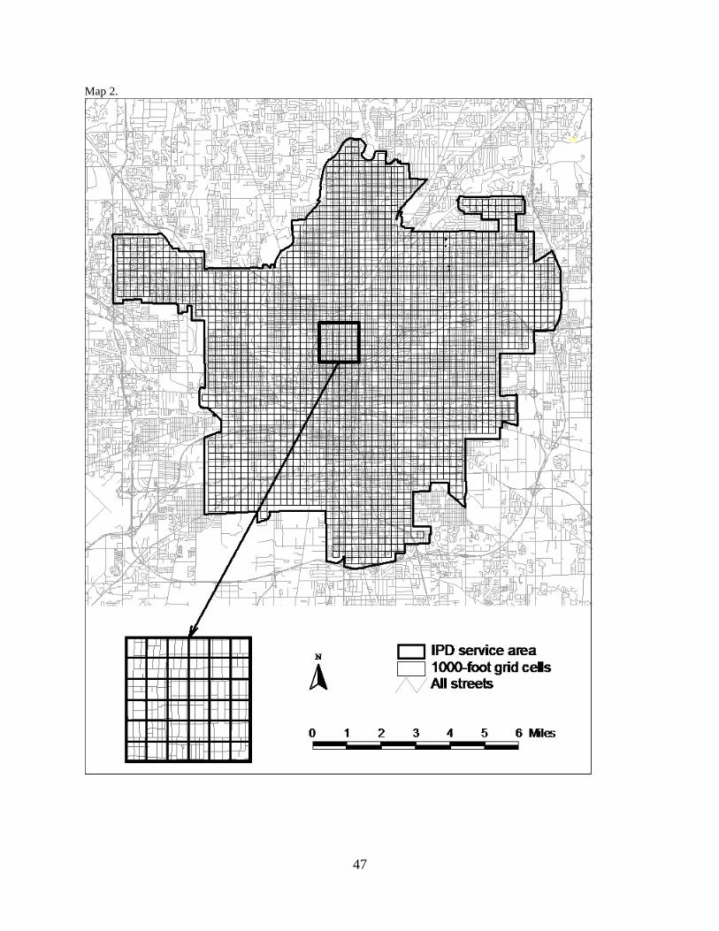
Map 2.
47
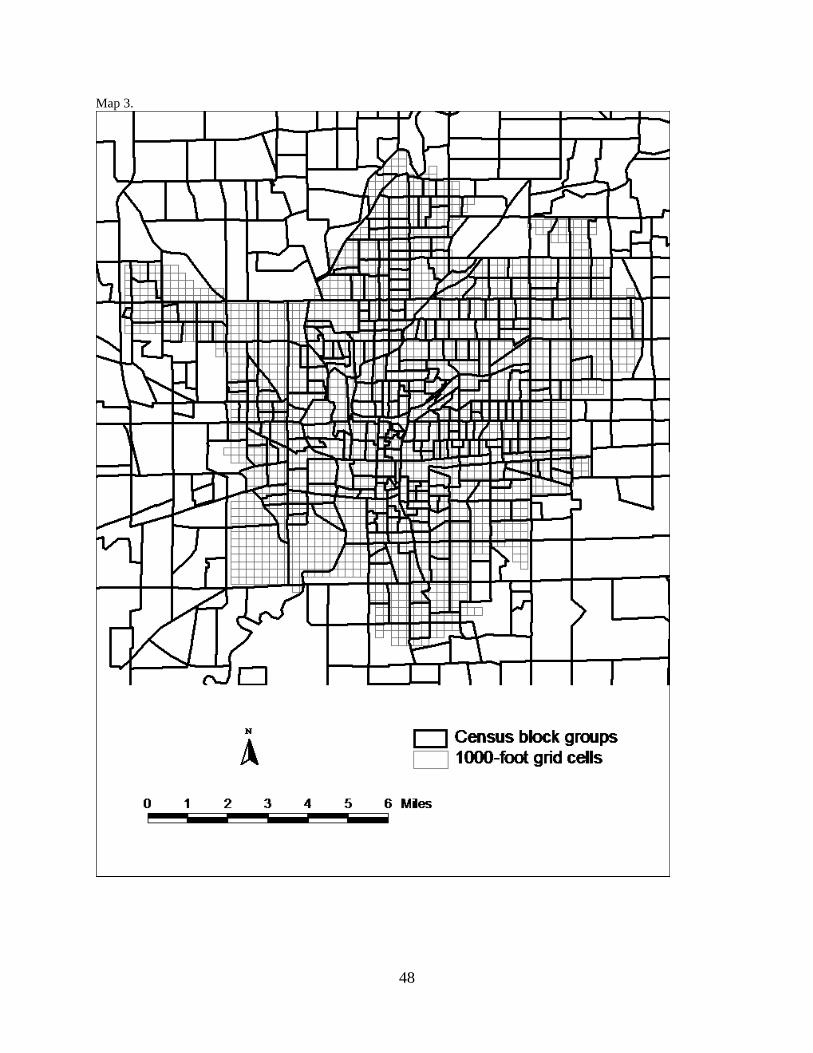
Map 3.
48