Land Use and Transportation Costs in the Brazilian … · Land Use and Transportation Costs in the Brazilian Amazon Eustaquio Reis IPEA, Rio de Janeiro Diana Weinhold♦♣ London

University of Wisconsin-Madison Department of Agricultural & Applied Economics

February 2004 Staff Paper No. 467

Land Use and Transportation Costs in the Brazilian Amazon

By

Eustaquio Reis IPEA, Rio de Janeiro

Diana Weinhold

London School of Economics Visiting Professor, Department of Agricultural & Applied Economics

University of Wisconsin-Madison

__________________________________ AGRICULTURAL &

APPLIED ECONOMICS ____________________________

STAFF PAPER SERIES

Copyright © 2004 Eustaquio Reis and Diana Weinhold. All rights reserved. Readers may make verbatim copies of this document for non-commercial purposes by any means, provided that this copyright notice appears on all such copies.

Land Use and Transportation Costs in the Brazilian Amazon

Eustaquio Reis IPEA, Rio de Janeiro

Diana Weinhold♦♣

London School of Economics

February 2004

preliminary draft, comments welcome ♦ We thank for very helpful comments and discussion Ajax Moreira, Newton de Castro, Lykke Andersen, and Brad Barham. We further thank all the seminar participants at the IX Seminário de Acompanhamento de NEMESIS in Rio de Janeiro, University of Manchester dept. of Economics, the University of Brisbane dept. of Economics, Monash University dept. of Econometrics, and the University of Wisconsin, Madison dept. of Agric.&Applied Economics. In addition we express our deep appreciation of the foundational inspiration and guidance of Clive W.J. Granger and our great joy at his recent Nobel prize. Of course all errors and omissions are our own. ♣ Correspondence to: Development Studies Institute, London School of Economics, Houghton Street, London UK WC2A 2AE Email: [email protected]

2

1. Introduction The Brazilian government’s Avança Brazil program has allocated over $3 billion for approximately 7,500 km of new Amazonian highways through 2007, prompting concerns about the effects on deforestation. In fact, the relationship between roads and land clearing is a question of intense interest to both environmentalists and policy makers in many regions of the world. Transport infrastructure improvements are considered to be one of the most effective tools for stimulating economic activity; at the same time environmentalists have largely condemned most road building as being one of the greatest threats to tropical forests. The construction of roads facilitates market access for crops, cattle and timber, opens up new areas for exploitation and decreases the costs of migration into forested areas. The degree to which this view has been integrated into the conventional wisdom is illustrated in Figure 1 below: the explanatory caption accompanying a NASA satellite photo of deforestation in Brazil reads “The pattern of deforestation spreading along roads is obvious [italics added] in the lower half of the image.”

In this paper we put forth some empirical evidence from the Brazilian Amazon that the relationship between roads and land clearing may be much more complex than the conventional wisdom implies. In particular we find that in areas that already at least partially cleared, improving the road network (i.e. decreasing transport costs) may actually decrease the rate of deforestation. We argue that our methodology of explicitly modeling the dynamics should be preferred to the more common static, contemporaneous analyses found in the literature. Furthermore, we endeavor to provide an encompassing explanation of our results. In other words, not only do we show that dynamic

modeling yields different conclusions from the conventional wisdom, but using our dynamic approach we are able to explain why so many other studies came to (possibly erroneous) conclusions using more traditional methods.

Figure 1. Satellite image of deforestation in the Amazon region, taken from the Brazilian state of Para on July 15, 1986. The dark areas are forest, the white is deforested areas, and the gray is regrowth. The pattern of deforestation spreading along roads is obvious in the lower half of the image. Scattered larger clearings can be seen near the center of the image. SOURCE: NASA

This paper proceeds as follows. In section 2 we briefly review the existing literature

on the relationship between roads and deforestation. Section 3 describes the data and the basic, dynamic functional form of the models. Section 4 outlines the basic econometric methodology used to estimate the dynamic models and discusses the results. Section 5 extends the analysis to rigorous out-of-sample causality/model evaluation exercises. In section 6 we reproduce the results of traditional contemporaneous correlation regressions and, employing insights gleaned in the previous two sections, show how these regressions may be severely miss-specified. Section 7 concludes and all results and tables are presented in the data appendix.

3

2. Brief Review of the Literature As discussed above, it is almost taken for granted in many circles these days that increased road building will increase deforestation. Indeed, the evidence for this conventional wisdom is compelling both empirically and theoretically. A number of studies have empirically documented a positive correlation between the extent of roads network and the degree of land clearing. For the Brazilian Amazon, Laurance et al. (2001) estimate that the effects of the Avança Brazil program will, in the optimistic scenario, increase deforestation by 269,000 hectares annually and release over $500 million worth of carbon emissions. Likewise Carvalho et al. (2001) also predict dramatic consequences of Amazonian highway construction. Many other studies also document a positive roads-clearing relationship; see, for example, Chomitz and Gray (1995) in Belize, Cropper, Griffiths and Mani (1996) in Thailand, Nelson and Hellerstein (1995) in Mexico, and Liu, Iverson and Brown (1993) in the Philippines, and Pfaff (1998) in Brazil. Anglesen (1999) explores four theoretical models of land use and finds that in three of them, improved roads do lead to more deforestation under a wide set of modeling assumptions. Concludes Anglesen, “…both this paper and empirical evidence suggest that lower access costs (roads) fuel deforestation” (p.211) However an emerging body of literature suggests that the relationship between roads and clearing may be somewhat more complex than the conventional wisdom implies. First, in theory at least, lower transport costs could either raise, lower, or have no effect on deforestation depending on the assumptions. Angelsen (1999), for example, shows that in a subsistence economy with no markets a decrease in transport costs will have no impact on clearing rates. Furthermore, Schneider (1994) and Chomitz and Gray (1995) both point out that (in theory at least) road intensification, as opposed to extensification, could possibly be a “win-win” strategy that both increases economic output while decreasing land clearing. According to this view, increasing the density of roads in already established market centers could raise productivity in those areas, concentrate economic activity and pull pressure away from more fragile, remote areas. Kaimowitz and Angelsen (1998) review the literature to investigate a related idea, that increased agricultural productivity could lessen pressure on the environment by allowing farmers to increase output on the same amount of land. In the end they remain highly skeptical of this possibility and point out that there are many examples where innovation has actually lead to increased land clearing. Mirroring the basic point of Schneider (1994) and Chomitz and Gray (1995), however, they refine this basic conclusion to allow for differing effects under different environments. In particular they comment,

… where the technological progress occurs is crucially important. If agricultural productivity is increased in an area not adjacent to forest and already under intensive cultivation or highly dependent on irrigation, the effect is generally good for conservation. But when farmers at forest edges have the means to increase their production cost-effectively, they generally have a greater incentive to clear more land to maximize output and income.” (Kaimowitz and Angelsen 1998)

Some recent empirical evidence has further supported the idea that the effects of roads may not be so clear-cut. In a study of land allocation decisions in the Ecuadorian Amazon, Pichon (1997) estimates that both total travel distance and total walking distance to an agricultural plot are positively related to the share of forest on the plot. Although this result by itself implies lowered transport costs would increase deforestation, he notes that the effects of walking distance were twice that of total distance; in other words, where plots were accessibly primarily by foot or canoe

4

only the forest clearing effect was much greater than more easily accessed plots. From these results he concludes that government policy could significantly reduce deforestation by improving transport infrastructure in areas that are already accessible, rather than expanding road networks into virgin areas. Muller and Zeller (2002) examine the relationship between road networks and land use in the highlands of Vietnam in both 1990 and 2000. They estimate a multinomial logit regression for each of four land use categories, lagging the exogenous variables (although not controlling for initial land use) to deal with possible endogeneity. Although their analysis is in levels only, and the distance coefficients in the forestry equations are not statistically significant, their overall conclusion from the analysis is that increased transport infrastructure actually led to increased forest cover. They explain,

“Access to all-year roads improved substantially in the last decade, thereby facilitating market integration, access to the infrastructure, agricultural inputs, and public services. The investments in irrigation and infrastructure, combined with improved access to roads, markets, and services, were successful in intensifying agricultural production. Higher agricultural productivity on existing land reduced the need for shifting cultivation, thus preserving forest cover while sustaining a much greater population on virtually the same agricultural land area.” (Muller and Zeller (2002) p. 347)

Mertens et. al. (2002) examine livestock and deforestation dynamics using Landsat satellite images from 1986, 1992 and 1999 in South Para state of the Brazilian Amazon. They examine four types of farmers: directed colonizers, small-scale spontaneous colonizers, medium-scale spontaneous colonizers and large-scale fazendas, estimating a multinomial logistic regression of the probability of deforestation for each type in each during the periods 1986 to 1992 and 1992 to 1999. Their empirical results on the role of ‘Distance from Main Road’ and ‘Distance from Secondary Road’ in predicting deforestation are highly mixed, with the majority of coefficients significant and negative (i.e. being closer to roads increases the chance of deforestation), but others (about 31%) are significant and positive, and the rest positive but not significant (12%). No obvious pattern over time or across the four categories of farmer is clear, but the authors soldier on, concluding that “the development and improvement of transportation infrastructure tends to be one of the most effective policy tools for influencing the spatial distribution of agricultural and forestry activities. But the role and impact of roads will depend on the type of road, the stage of development of the frontier area, and roads will affect the various types of producers in different ways. (authors’ own italics, p. 291) Although the theoretical arguments that increased roads might decrease deforestation under some circumstances are compelling, it would be fair to observe that the empirical evidence reviewed above is weak at best, especially compared to the seemingly overwhelming evidence of numerous other studies showing a positive relationship between roads and clearing. Furthermore, any successful challenge to a well established result bears the burden not only of demonstrating robust conclusions, but it should also be an encompassing study in that in addition it should be able to explain why previous studies obtained the results that they did. One characteristic that all the studies reviewed above share is that they are more or less static, examining the (usually) contemporaneous relationship between the levels of transport costs and the levels (i.e. extent) of cleared land (or probability of clearing). For example, Laurance et al. (2001) overlays the 1995 road network on a 1992 map of the Amazon and for each section of highway calculates the extent of clearing within certain defined zones to each side of the road. Thus they

5

causally attribute all of the cleared land to the road in question. However two more recent studies, by contrast, have estimated explicitly dynamic models of land use in the Brazilian Amazon. In Andersen et. al (2002) we and other co-authors analyzed an extensive data set of land use and economic activity in 257 municipalities of the Brazilian Amazon from 1975 to 1995. Several parts of our book relied on developing a model of the dynamics of land clearing and economic activity and one of the policy variables was roads, both paved and unpaved. Thus a key policy question was the relative importance of road building in land clearing (as well as economic development) compared to other possible causes. Given the evidence cited above, a priori we expected that paving roads (i.e. decreasing transport costs) would increase economic development, but at the cost of increased land clearing. We hoped to quantify this trade-off explicitly in a fashion that had not yet been accomplished in the literature. However to our surprise the result that fell out of this analysis was that past increases and levels of federal and state paved roads seemed to be correlated with decreased land clearing overall, but with the exact relationship depending on the extent to which a region was already settled. In particular, an interaction term between paved roads and level of cleared land showed that the strongest decreases in clearing rates occurred in areas that were already settled, while the net effect of paving roads in more pristine areas was more likely to be detrimental to the forest. However, even allowing for differential effects of roads depending on the extent of existing clearing, with our data and methodology the estimated overall net effect of the actual paved roads across the whole Amazon was still negative (i.e. lower clearing rates). Although, as we have discussed, this result is consistent with some theoretical ideas that have been proposed, the magnitude of our results was contrary to most all existing studies and flew directly in the face of conventional wisdom on the topic, leading several experts to sharply question their validity. Nevertheless ours was not the only study to produce these results. Independently, Dr. Ajax Moreira using the same DESMAT data, but different variables for transport costs and a different econometric estimation methodology (a spatial VAR model), came to much the same conclusions as we did regarding the relationship between transport costs and land use. Moreira (2003) finds that decreasing transport costs increases agricultural productivity and cattle herd density, and lowers the rate of land clearing. Dr. Moreira’s results were similarly assailed by critics, so each team was astonished to hear of the others’ results at a recent conference in Rio de Janeiro. While two studies that employ essentially similar data may not constitute a serious enough challenge to change conventional wisdom unconditionally, there are good reasons not to dismiss these results out of hand too quickly. In particular our (and Dr. Moreira’s) analyses took advantage of time series and spatial information at a level of disaggregation that is unusual for this literature. As discussed above, most of the other studies that have been done to date are based on snapshots of data at single points in time. If roads really do increase the rate of deforestation, then we should observe that roads constructed in time t are associated with increased clearing over the next time period. The advantage of our data set is that we have information across all municipalities in the Amazon over a long period of time, from 1975 to 1995. Thus we can more effectively address issues of causality by exactly asking these kinds of time-conditional, dynamic questions about the relationships between variables. 2. Data and basic dynamic functional form of the models Although we would strongly advocate our approach as superior to contemporaneous, levels-based analysis, this paper is not meant as a defense of our roads results as described above. In fact there were a number of problems with the roads that data that we discussed in the book. In particular,

6

our measure was of the extent of roads in a given municipality and as such we could not distinguish between roads that connected valuable markets and roads that simply ran in circles. Recently, however, we obtained much improved data on transport costs across the Amazon. At IPEA in Rio de Janeiro. Dr. Newton de Castro has used GIS analysis to compile an extensive data set on municipality level transport costs both to local markets and to Sao Paolo –in fact it was this data that Dr. Moreira used in his study. For each municipality in each period of time examined, Dr. Newton mapped out the most cost-effective route to each market, respectively. The remaining data available for the book and this study was extracted from a large database on economic, demographic, ecological and agricultural variables (mostly from the Brazilian agricultural census administered by the Brazilian Statistical Office (IBGE)) maintained by Dr. Reis at the Institute for Applied Economic Research (IPEA) in Rio de Janeiro. Hundreds of variables of ecological, economic and agricultural conditions have been collected for the years 1975, 1980, 1985 and 1995 for 257 consistently defined areas1 in the Brazilian Legal Amazonia (some data for 1970 is also available, but not utilized in this study). As mentioned above, Dr. Newton de Castro at IPEA provided the transport cost data that he compiled. Our endogenous (dependent) variables are growth of cleared land, rural and urban GDP growth, rural and urban population growth, cattle herd growth and cattle herd density, and growth of transport costs both to Sao Paolo and to local markets. Although these two measures of transport costs are correlated (with a correlation coefficient of .64 in levels and .22 in growth rates) they also embody very different information. For the most part, roads towards Sao Paolo run north-south, while roads to local markets are more likely to run east-west. We use growth rates for our endogenous variables for several reasons. First, the levels are highly trending in most of our variables and thus a model in levels would be highly susceptible to spurious correlation. Second, by taking growth rates we effectively eliminate the municipality-specific levels “fixed effects” from the analysis. Controlling for the fixed effects in levels also controls for the overall average level of spatial correlation in the data, thus cutting down considerably the scope for spatial correlation becoming a problem in the estimation. We condition on a once and twice lagged dependent variables and a thrice-lagged initial level of each endogenous variable in the specification. By using only lagged variables we attempt to minimise the potential of endogeneity problems. Furthermore, these lagged (log) level variables embody all the information that was important for determining the endogenous variable at that time (1975), including unobservables. Using model evaluation (discussed below) criteria we have elected to separate the model by years rather than pooling. Thus, our final specification is actually a cross section (albeit with a lot of time-series information included) rather than a panel, which has the advantage of avoiding some of these statistical problems that arise with very short dynamic panel estimation. Some time-invariant municipality-specific characteristics could still play a role if they are important determinants of the growth of our endogenous variables, not just the levels (i.e. “fixed effects” in growth rates). Thus we include a number of time-invariant variables including a full set of state dummy variables, measures of the original natural vegetation and soil type of each municipality, distance to state and federal market, length of navigable river, variables on the average monthly temperatures, and a dummy variable for high rainfall. 1 These areas are roughly equivalent to municipalities (or counties) which may contain both urban and rural populations, but while the borders of legal municipalities have changed over the time span of the study, the borders of the 257 regions have been defined so as to be constant over time.

7

Finally, in the frontier environment of the Amazon spatial location can be extremely important in determining economic activity. While controlling for levels fixed effects helps to absorb much of the levels-spatial correlation in the data, we also include additional spatial variables which measure the state of affairs along a number of dimensions in nearby municipalities. In particular we control for the (lagged) level of all of the endogenous variables, normalised by land area where appropriate. Each spatial variable is constructed by taking the weighted average value across the five closest neighbours, with the weights inversely proportional to the distance between them. 4. Basic dynamic models: econometric methodology and discussion of results 4a. econometric methodology Given this wealth of data, the task of specifying a model to estimate becomes a problem of too much, rather than too little, choice. Our list so far includes (twice) lagged growth and initial (log) levels of the endogenous variables, a set of municipality-specific characteristics, a set of spatial terms and roads and land price data for a total of 74 initial variables. With a sample size of 257 it is clearly impractical to include all the variables in a final regression; but any smaller subset of these variables chosen from theory would run the risk of omitting potentially important factors With an enormous wealth of possible variables to choose from, and a very emotionally charged topic of study, in Andersen et. al. (2002) we were particularly sensitive to the possibility of bias influencing the choice of variables and the results. In fact, even if we could manage to be completely objective any conclusions we might reach might be susceptible to accusations of author-bias unless we could document carefully our methodology and make it as objective and accessible as possible. To that end we based our approach on a series of model evaluation exercises to determine initial functional form, and then developed a new, automated “general to simple” approach to reduce the large initial number of possible explanatory variables to smaller “final” models (see discussion of random reduction below), all without any interference whatsoever from any of us. Furthermore, even without the prospect of subtle author-biases, the processes of growth and development in the Amazon are clearly complex and evolving over time as the role of government policy changes and the frontier advances. A good structural model of these processes requires a comprehensive theoretical knowledge of the possible important relationships; leaving out any one of them could significantly bias the results if the processes under study are correlated with the omitted variables. However, identifying all the dynamic and spatial interactions and feedback relationships that could be expected to play an important role in the evolution of these processes is virtually impossible. We therefore estimate a reduced form model in which we start with an initial (large) set of variables which may play a role and let the data itself decide which of those should be included in the model: the so-called `general to simple' modelling strategy (for a complete discussion see Hendry 1995, pp.344-368). In this paper we reproduce the functional form and basic set of initial control variables from Andersen et. al (2002) with the only difference being that we substitute Dr. Castro’s transport cost data instead of the original roads variables. Having chosen our preferred general to simple methodology and settled on a functional form and set of initial variables for our general model we now turn to the question of estimation. As we have discussed above, the basic estimation strategy upon which our methodology is based is a Hendry

8

model reduction procedure in which a general model is initially estimated and variables found not to be statistically significant are sequentially deleted, keeping an eye on model performance, until a final, parsimonious model is obtained. However, in general models generated in this manner face a major problem in that the actual sequence of reduction can be somewhat arbitrary, such that several different but equally “good” models could legitimately be derived from the same starting point. Furthermore at this point there is quite a bit of room for discretionary actions by the researcher both in terms of the reduction sequence as well as deletion criteria. Even with the best of intentions subtle biases can enter the process. In order to avoid these problems we utilise an approach called “random reduction” estimation (see Weinhold 2001, Andersen et. al. 2002). For each model we start with an original set of possible explanatory variables as outlined above. The model selection then proceeds as follows. 1. The model is estimated and heteroskedasticity and autocorrelation consistent standard errors are

calculated. In the case of a single time observation these are simple Huber-White standard errors. (If we were to estimate the model with multiple time periods we would also want to control for possible autocorrelation in the errors by using a HAC (heteroskedasticity and autocorrelation consistent) estimator.)

2. First we delete observations for which the error term in the unreduced model is more than three

standard deviations from the mean so that these outliers do not unduly impact the estimation. 3. Then the program finds the three lowest robust t-statistics that are under 2.0 in absolute value. It

then selects randomly between these three t-statistics and deletes the corresponding variable from the RHS of the equation. In the case that there are only two t-statistics under 2 (in absolute value), the program randomly chooses one of these. If there is only one t-statistic under 2 then the corresponding variable is deleted. The model is then re-estimated as per step 1.

4. This process continues until a specification is found which fulfils some criteria of a “good”

model. In our case the criteria we have selected is that all variables have Huber-White robust t-statistics of at least 2.0, i.e. that they are statistically significant at the 5% level of significance. One could legitimately question this criteria as the true size of the final t-statistics are unknown because they are the result of a purposeful search, not a one-off hypothesis test. An alternative approach would be to search over different model specifications and select variables not on the basis of individual t-statistics but of some overall model selection criteria such as adjusted R-squared, AIC, BIC and/or other selection criterion. However, starting from a very general specification and using this approach to reduce the number of explanatory variables is very computer-intensive as the number of possible alternative models is enormous. Given that our methodology already relies on computer-intensive iteration this approach was deemed to be computationally infeasible in the time available.

5. The whole process is repeated again from the start, resulting in another final model that,

because of the randomisation of the reduction process, may be quite different from the first one. We continue to repeat the whole process 100 times so that we have 100 “final” models.

6. We then count how many times each variable appears in a final model. In addition we can

observe the lowest and highest value that each variables' coefficient takes. This gives us a sense of how stable the coefficient value is across the different patterns of reduction that could occur.

9

4b. Random reduction results In table 1 we note that some robust determinants of the growth of cleared land are the growth of urban and rural populations, both of which increase growth of cleared land. Areas with established, relatively high rural GDP also have increased rates of land clearing. However, growth of urban GDP is associated with lower rates of clearing (remember we are controlling for population). This is consistent with the idea that as urban activity increases, agricultural land use could intensify and demand for new cleared land could thus decline. The growth of cattle herds also increases cleared land, a finding consistent with most of the literature which points to cattle ranching as the primary cause of deforestation and land clearing in the Amazon. Transport costs are also a significant determinant of the pattern of new land clearing. Contrary to conventional wisdom, we find that decreased transport costs to local markets decrease the rate of land clearing. The relationship between land clearing and transport costs to Sao Paolo is more complex. Both the level of transport costs to Sao Paolo and the interaction term associated with that variable are highly robust. Thus although lower transport costs to Sao Paolo are associated with higher growth rates of clearing for areas with low initial levels of cleared land, for those municipalities with higher shares of cleared land we find the contrary, that lower transport costs to Sao Paolo decrease the rate of clearing. If we look at the marginal effect of transport costs municipality-by-municipality we find that for some municipalities the total marginal effect of transport costs turns out to be negative, and for some it is positive (the marginal effect varies between -7.05 and +10.33). If we calculate the total marginal effect of the level transport costs to Sao Paolo on all municipalities in the data set, we get a mean (positive) value of 1.45. Thus, on average, lower transport costs to Sao Paolo lower the rate of land clearing, which is consistent with the results obtained (less robustly, not reported) when interaction terms were not included in the initial general model, and is also consistent with the results we obtained in Andersen et. al (2002) using the same methodology and data on paved roads. Given the complexity of the relationship we do not want to emphasize this average result, however; it is more important to note the heterogeneity across municipalities. It suggests that improvements in transport infrastructure could have very different consequences for the environment depending on where they are located. Results from the growth of cattle herd are reported in table 2. Very few variables are robustly correlated with growth of cattle herd, suggesting a poorly specified model with a fair amount of omitted variables. Consistent with this result, Moreira (2003) also finds that the cattle herd is unstable and thus vulnerable to exogenous stimuli. In any case, of those few variables that do regularly make it into the final models, the past growth of cleared land is robustly and positively correlated with the growth of cattle herd, suggesting that in the relationship between cattle and deforestation, causality could operate in both directions. However perhaps the most robust determinants overall of the growth of cattle herds is the evolution of transport costs, although transport costs to Sao Paolo and to local markets seem to play very different roles. Both the growth of transport costs to Sao Paolo, as well as the interaction of this variable with cleared land, are extremely robust. Overall the mean marginal effect of growth of transport costs to Sao Paolo on the growth of cattle herd is negative (with a mean value of –1.620); in other words, as transport costs decrease the growth of cattle herds increases. However, since the interaction term is positive, this suggests that in those municipalities with high levels of cleared land, decreased transport costs to Sao Paolo could lower the growth of cattle herds. Indeed, for some municipalities the marginal effect of transport cost does indeed turn out to be positive (the value of the marginal effect of transport costs on cattle herd growth varies between –8.8 and +5.9).

10

The role of transport costs to local markets is quite different. Overall, lower levels of transport costs to local markets is associated with lower growth rates of cattle herd (with an overall mean marginal effect of +2.11). However in some municipalities that are already highly cleared, lower transport costs to local markets are associated with higher rates of growth of cattle herds. Both of these results point to very different dynamic relationships between transport costs and economic activity in highly cleared areas, and less cleared areas. The impact of cattle on both economic activity and land clearing are determined not only be the extent of cattle ranching, but also by the herd density (or intensity) which we model in table 3. The model of the growth of cattle herd density also has a problem with few robust variables. Areas that are already highly cleared have higher herd density. Other than endogenous dynamics, the only other variables that are robustly correlated to herd density are transport costs. Past growth of transport costs has a negative effect; in other words as transport costs decrease, density of cattle herd increases. The interaction term of this variable with cleared land is positive, however, so that for municipalities with very high proportions of already cleared land, lowered transport costs could lead to lower herd density. However the overall mean effect is still negative (lowered transport costs lead to higher herd density). The distribution of the aggregate marginal effect of growth of transport costs to Sao Paolo, a mean of –3.36 with a standard deviation of 3.11 and a span of values from –11.733 to +5.39, suggests that the relationship is indeed negative for the larger share of municipalities, going positive in only those municipalities with the very highest levels of cleared land. The relationship between herd density and transport to local markets is again quite different. Both the level of transport costs to local markets as well as the interaction term with cleared land for this variable are robust. The overall mean marginal effect of level of local market transport costs turns out to be positive, at +1.60, implying that municipalities with lower local transport costs have lower herd densities. However, again the interaction with cleared land refines this interpretation. The interaction term is negative, suggestion that among those municipalities with high proportions of cleared land those that have lower local transport costs also tend to have higher densities of cattle herds. Table 4 presents the results of the Random Reduction procedure applied to the model of rural GDP growth. Robust positive determinants of growth of rural GDP include growth and level of cleared land, with neighbors’ cleared land proving an economic attractant and pulling economic activity away. Growth of urban population also has a strong positive effect, reflecting the emergence of endogenous market forces driving many outcomes now in the Amazon. In table 5 we observe that the model for the growth of urban GDP is remarkably stable, with almost all of the 100 final models sharing a similar set of RHS variables. The primary driving forces of urban GDP growth are (not surprisingly) urban population growth and level, including the presence of urban population in neighboring municipalities as well. Urban areas with nearby substantial cattle herds also grow faster, and past land prices also are associated with higher growth. While transport costs seemed to have little impact on growth of rural GDP, it plays an important role for growth of urban GDP. In particular, lower transport costs to local markets are associated with higher urban GDP growth. In addition lower transport costs to Sao Paolo (via neighbors) also raises urban GDP growth. However, lower transport costs to local markets in neighboring municipalities seems to exert a diverting force, pulling economic activity away.

11

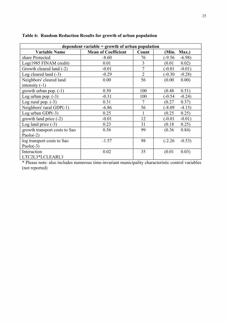
Tables 6 and 7 present the results from the random reduction of the models of growth of urban and rural population. For the growth of urban population (table 6), aside from endogenous dynamic terms the only other robust variables are transport costs. In particular, as expected we find that municipalities with relatively lower transport costs to Sao Paolo have relatively higher growth rates of urban population. However, in those areas where transport costs to Sao Paolo have been decreasing fastest, urban population growth has actually been slower. In the model of rural population growth (table 7) very few variables are extremely robust, but a few make into the final model with some regularity. The evolution of urban populations seems to have a very important effect, with rural populations growing more in municipalities with large, and growing, urban populations. However where urban GDP is relatively low, the urban attractant is not as powerful and this seems to increase rural population growth. Finally, as with urban population growth, the distribution of transport costs is crucial for the pattern of rural settlements in the Amazon. The most robust relationship between transport costs and rural population growth is for growth of transport costs to Sao Paolo. Where these transport costs have been declining the fastest, rural populations have increased the most rapidly. The interaction term with cleared land for this variable is also robust and positive, suggesting that in those municipalities that are highly cleared, decreasing transport costs to Sao Paolo has actually been associated with lower rural population growth. Although the overall mean effect is very slightly negative, the distribution of the total marginal effect of growth of transport costs to Sao Paolo on rural population growth suggests that for about half the municipalities the effect is positive, and for about half it is negative. (The overall coefficient itself has a mean of -0.003, a standard deviation of 0.303 and a min – max value span between -0.82 to +0.85.). Finally in tables 8 and 9 we examine the determinants of the growth of transport costs, both to Sao Paolo and to local markets. From table 8 we observe that the evolution of transport costs to Sao Paolo seems not to be governed my much beyond its own internal dynamics and the evolution of local market transport costs (although oddly we find lagged growth of rural population to be positively associated with growth of transport costs). Transport costs seem to be declining fastest in areas where costs were initially the lowest in any case. Where costs to local markets are low, we find that costs to Sao Paolo are declining as well. However both robust interaction terms are negative, suggesting that this relationship does not hold as much for areas that are highly cleared already. In particular among the most highly developed (i.e. cleared) municipalities we find that transport costs are providing an equalizing force, decreasing faster in those areas with initially higher costs. The evolution of transport costs to local markets, presented in table 9, are declining as growth of cleared land increases, and as urban (and to a lesser extent rural) population increases. A very robust finding is that higher levels and rates of growth of rural GDP is associated with higher transport costs to local markets, a counter-intuitive finding that probably (??) reflects the fact that urban activity is more likely to displace rural agriculture when transport costs are lower. Indeed, although not very robust we do find that urban activity is associated with lower transport costs to local markets. Again, while transport costs to local markets are decreasing faster in areas with already low transport costs, in those areas that are highly cleared this relationship reverses itself, with transport costs decreasing faster in municipalities with higher transport costs. 4c. summary of general estimation results In sum, we find broadly similar results as those we obtained in Andersen et. al (2002) using an identical methodological approach but data on paved and unpaved roads, rather than direct measure

12

of transportation costs. In particular, in areas with established populations and economic activity the reduction of transport costs can intensify cattle ranching and decrease new land clearing. On average for the whole Amazon the relationship between transport costs to Sao Paolo and new clearing is positive; the lower the transport costs the less the new clearing. However we don’t want to read too much into this aggregate result as it masks considerable variation across municipalities. In particular we find strong evidence that those municipalities with relatively low levels of initial clearing will experience increased clearing in response to decreases in transport costs, while settled areas may experience a smaller increase or even a decline in clearing rates. 5. Testing For Causality While our estimates so far have broadly confirmed the conclusions from our book’s analyses, we would like to go further and impose increased scrutiny and analysis on this question. In Andersen et. al. (2002) the roads result fell out of a more general methodology designed to accommodate multiple objectives; in this case our sole objective is to study the relationship between transport costs and land use. To that end we subject our transport cost and clearing data to a series of out-of-sample model evaluation-based causality tests. We adopt a definition of causality that revolves around the relative power of models to forecast into the future and as such entails an intrinsically time series approach. With panel data, in-sample fit and contemporaneous correlation may come from either the time-series or the cross section variability in the data. Thus to interpret the results from such an exercise as indicative of dynamic causality demands the assumption that all the cross section units are evolving along similar paths and simply represent different stages of the same basic process but at different points in time. In this exercise we adopt much stricter, more direct test of dynamic causality more closely tied to the time-series, out-of-sample forecasting properties of the model. In particular we estimate a series of models of growth between 1985 and 1995 of some key variables of interest (such as cleared land), conditioning only on time invariant municipality characteristics as controls, lagged information on the dependent variable and lagged growth and levels of other variables of interest (such as transport costs). We then compare the out-of-sample forecasting ability of this model to an analogous, sister model that includes the information on the dependent variable but omits the information on the candidate causal variable. If the former model performs statistically significantly better out-of-sample, then we find evidence of causality. It is, however, important to keep in mind that our definition of “causality” is a very specific, dynamic order concept. True underlying structural causality could actual be the reverse of that observed if forward looking agents make decisions on the basis of expectations (i.e. buying baby carriages does not cause childbirth). We consider the possible implications of this limitation in the discussion below and try to control for it as best our data allows. We have data on transport costs for 1975, 1985 and 1995. Thus when we condition growth between 1985 to 1995 on only past values, for transportation costs this implies that we have unique information only for the growth from 1975 to 1980 (technically 1985, but 1980 is interpolated in the data and embodies all the information we need, and so to keep notation consistent we adopt this), and the level of transport costs in 1975, in other words growth lagged twice and level lagged three times. For growth of cleared land and growth of urban and rural GDP we have complete data and so condition on the first and second lagged growth rates and the log-level lagged three times. We further include variables to capture spatial, neighborhood effects which are the weighted average of the lagged log-levels of neighbors’ values of a variable, suitably normalized where

13

appropriate. Finally, as we have found that the interaction between transport costs and level of cleared land potentially carries a lot of information, where appropriate we condition as well on lagged interaction terms (remember, however, that the second model must contain no information on the second variable). Consider the following two models; in this case we have written them as though variable 2 corresponds to transport costs, so there is only one growth lag (if variable 2 were cleared land or GDP, there would be two lagged growth terms).

∑ ++

+++++++++=

kiikk

iiiiii

iiiiii

C

LclearLvar2LclearGvar2Lvar2SpLvar2Gvar2Lvar1SpLvar1Gvar1Gvar1Gvar1

1

7575975808857756

80585475380285195

)*()*(__ (1)

εγ

βββββββββα

∑ +′+′+′+′+′+′=k

iikkiiiii CLvar1SpLvar1Gvar1Gvar1Gvar1 185475380285195 _ (2) εγββββα

Where Cik denotes time-invariant municipality specific control variables, which in this case include a set of state dummy variables, municipality size, distance to state and federal capital, and a CITY dummy for large urban municipalities. Models (1) and (2) are two competing models of variable 1; model (1) includes information on past growth rates and levels of both variables in question, while model (2) includes only lagged endogenous and control variables. Thus, for example, if model (1) can forecast more accurately than model (2) we can deduce that information about the past of variable 2 was important. If, on the other hand, model (2) forecasts better than model (1) or there is no difference, then we conclude that including information about variable 2 does not help to predict growth of variable 1 and therefore there is no causal relationship. We focus on out-of-sample forecasting to avoid problems with over-fitting in-sample estimation. Thus by determining which model from each pair displays superior out-of-sample forecasting performance , we can determine whether there is evidence of any causal relationships between the two variables of interest. We turn to panel model evaluation techniques suggested in Granger and Huang (1997) to determine whether the difference in forecasting ability between the models is statistically significant. In particular, following Granger and Huang (1997) we adopt a classic sum-difference test which takes the following form. Consider the forecast errors η1it and η2it from models (1) and (2) where j and t denote not-in-sample cross section municipalities and time periods. The null hypothesis is: HO: η η2

12

2it it= It then follows that if HO can be rejected then the model with the lowest forecast error variance should be accepted as being significantly superior to the competing model. To this end Granger and Huang suggest constructing the following variables: SUMDIFF

i i

i i

12 1 2

12 1 2

= += −

i

i

η ηη η

Then a test of the null hypothesis is equivalent to a test of whether δ = 0 from the regression:

14

SUM DIFFi i12 12= + + iα δ ξ The procedure is outlined in Weinhold and Reis (2001). More specifically, the sum-difference test is more fully discussed Granger and Newbold (1987), Mincer and Zarnowitz (1969), and more recently in Diebold and Mariano (1995). An important limitation of the data is the availability of only 4 time observations (1975, 1980, 1985 and 1995) on the level variables for cleared land and GDP, and only 3 time observations (1975, 1985 and 1995) of the levels variables on transport costs in each municipality. This is not quite as big a problem as it seems at first; since the observations are 5 or 10 years apart each data point embodies a lot of unique information. (In other words, the data are not as correlated as annual data would be.) When considering long-run relationships such spread-out data can be adequate. However, if the periodicity of the relationship in question is less than 5 years on average, then we will not be able to detect important aspects of the dynamics. We take logs and first-difference the data to generate either three or two observations of the growth rate of each variable for each municipality2. Of course, the fact that we have only three or four original time observations makes estimation difficult in any case but we believe that our methodology is fairly well adapted to such situations. We do not rely on precise estimates of parameters but are rather running a model competition in which all models are equally handicapped by the scarcity of time series observations. 5b. discussion of causality results In tables 10 and 11 we present a series of model evaluation exercises examining the relationships between transport costs and our key variables of interest: land clearing, urban GDP and rural GDP. If the mean squared forecast error of model 1 is smaller than that for model 2 it implies that the information from the candidate causal variable was useful. The t-statistic of the difference tells us if the difference this extra information provides is statistically significant or not. It is important to point out that these exercises do not tell us about the aggregate sign of the relationship in question, only whether the information embodied in the variables decreased the out-of-sample forecasting ability of the model. We rely on additional analysis (i.e. analyses such as that reported above) to ascertain the sign. Another important thing to note is that a model evaluation exercises is a very different, and arguably much harder test to “pass” for a variable, than standard in-sample statistical correlation. In fact, in an analogous exercise using our old roads data, none of the model evaluation comparisons in any direction were statistically significant. Thus relationships which were statistically significant in our in-sample regressions may not turn out to be here, and vice versa. In addition, our set of control variables here is considerably more limited. Table 10 presents the results that are most analogous to our random-reduction model in that we model growth from 1985 to 1995. Although including transport costs in the model of cleared land does improve out-of-sample model performance slightly, this difference is not statistically significant. The model evaluation test do soundly and significantly reject the hypothesis that rural GDP has any causal relationship to the growth of transport costs to Sao Paolo. More profoundly

2 At the same time this process eliminates the effects of time-invariant municipality-specific characteristics on the levels relationship (i.e. the so-called "fixed effects").

15

for our purposes, however, is that we find that past information on cleared land significantly improves our ability to forecast (out-of-sample) changes in transport costs. Many sceptics have rightly pointed out that road building in the 1985 to 1995 period was less than the historical norm and that this time period might not be representative. In addition, changes in cleared land between 1985 and 1995 tend to be underestimated due to differences in the census collection dates. In as much as this potential bias affects all municipalities equally (or at least all municipalities in each state equally) it would not be a problem, but we cannot be sure of this. Thus for our most important relationships in question, that between transport costs and cleared land, we re-do the analysis for the 1980-1985 period and present the results in table 11. Due to data limitations as described earlier, the lagged conditioning information for transport costs comprises just the lagged level (no growth rates). We find the results are very similar. Again, the information on transport costs improves the model of cleared land, and for this period the t-statistic on the difference is larger, but still not significant. At the same time both models explaining the evolution of transport costs are significantly improved by information on past clearing. Overall we find stronger evidence that land clearing patterns predict road improvements than the reverse. This could be because clearing causes roads to be built or improved; or it could result from settlers’ expectations of future road construction causing them to clear land in advance (or both explanations could be partially true). It is admittedly difficult to control for this latter possibility; however we do have information on (lagged) land prices (these were included as possible control variables in the random reduction regressions above). In as much as these prices embody settlers’ beliefs about future improvements, then, including them in the analysis may go some way towards controlling for expectations. Thus we re-do the model evaluation exercises for transport costs and land clearing, controlling for information on land prices in both the models including and excluding the candidate causal variables. Our results (not reported) are almost identical to those discussed above; information on road building improved the out-of-sample prediction of land clearing but not statistically significantly. On the other hand, even controlling for information on land prices, clearing patterns did significantly improve our prediction of future transport cost changes. Although our evidence suggests the story is not being driven primarily by expectations, the variable quality of the land price data and rather long time spans involved would caution against drawing too hasty a conclusion. The role of expectations and price speculation in land use choices is a complex issue and a fertile area for future research. 6. Traditional contemporaneous analyses: an encompassing explanation The results from our model evaluation exercises suggest that land clearing activity causes changes in transport costs, rather than the reverse. If this is in fact the case, then any contemporaneous regression of land clearing on transport costs will suffer from endogeneity bias. This in turn raises the startling possibility that the causal relationship underlying the commonly observed contemporaneous correlation observed between cleared land and roads has been interpreted (at least partially) incorrectly. We investigate this possibility by first reproducing the common finding that lower transport costs are associated with greater land clearing. Column (1) of table 12a presents just such a regression of contemporaneous correlation between growth of cleared land and growth of transport costs. Growth of newly cleared land is positively and significantly correlated with decreasing transport

16

costs to Sao Paolo. Thus this would seem to support the traditional idea of lower transport costs leading to increased land clearing. However, our model evaluation exercises strongly suggested that causality in fact runs in the opposite direction, in which case the regression in column (1) would be misspecified and suffer from endogeneity bias. Thus in columns (2) and (3) we instrument for transport costs using lagged information on transport costs and paved and unpaved roads. The list of instruments and first-stage R-squares are reported in table 12b. The instrument set seems quite good as the R-squares from the first stage regressions range from about 0.6 to 0.8 for the growth of transport costs, and reach 0.99 for the levels variables. Arguably past values of roads are likely not to have been caused by future growth of cleared land, and the system also passes a standard overidentification test. Once we have instrumented for growth of transport costs in column (2), not only does growth of transport costs to Sao Paolo lose all statistical significance, the coefficient estimate actually changes signs! The (uninstrumented) level of transport costs to Sao Paolo remains slightly significant, however, and is still negative. In column (3) we instrument for all transport cost variables and all these variables lose statistical significance. Our random reduction model suggested that the interaction between transport costs and levels of cleared land is potentially a very important aspect of this relationship. Thus in table 13a we present this regression again, this time including the similar interaction terms we used in the random reduction models. Column (4) presents the OLS results. In this case levels of significance for the transport cost variables are greatly reduced from those in table 12 and the pattern is similar to those detected in the random reduction model. In particular, decreased transport costs lead to increased land clearing, but in municipalities with high levels of cleared land this effect is diminished or even reversed. Again, however, if causality runs in the opposite direction then this OLS regression will be biased. Thus in column (5) we present the same regression with all terms that include transport costs have been instrumented for (first stage information presented in table 13a). Using IV estimation none of the transport variables are statistically significant anymore. 7. Conclusions and Discussion One cannot overstate the policy importance of obtaining reasonably accurate estimates of the effects of road improvements on both economic activity and land clearing in the Amazon. The Brazilian government has earmarked billions of dollars over the next decade for road construction and paving through the region under the Avanca Brasil plan and the future of the Amazon forest, and the well being of its many human inhabitants, will be significantly effected for better or for worse accordingly. A better understanding the relative trade-offs between economic growth and environmental damage will greatly enhance the ability of policy makers to design more sensible road systems that are consistent with societies’ values (which society’s values is another paper(!)). That a very strong, robust correlation exists between the level of clearing and the level (i.e. extent) of roads cannot be denied. However, on the basis of this strong levels-correlation very strong conclusions have been drawn about the causal nature of this relationship. Unfortunately, though, a strong levels-correlation accompanied with a plausible sounding theory does not prove that causality goes only from roads to land clearing (though undoubtedly this is a large part of the story). There could also be feedback between the two variables, with reverse causality playing a role in the final observed static correlation. Thus in this paper we have taken a rich data set with both time series and spatial variation at the municipio level for legal Amazonia and subjected it to battery of more rigorous tests.

17

We specify dynamic rather than static models, difference out levels fixed effects, and condition on past variables to minimize endogeneity. We further allow for municipio-specific heterogeneity in the relationship between transport costs and land clearing. In the first instance we follow Andersen et. al (2002) and use an automated “random reduction” technique for dealing with a large number of candidate explanatory variables without possibility of bias or interference from the researchers. These regressions suggest that decreasing transport costs in cleared areas will indeed increase deforestation in areas of virgin forest and natural land cover. However, our results also suggest that in areas with established settlements this relationship could be significantly modified or even reversed, with lowered transport costs lowering the future rates of land clearing. We then subject the transport cost and land clearing variables to a series of strict out-of-sample forecasting exercises to ascertain whether past information of each variable is useful in predicting the evolution of the other variable. We find consistent evidence that the evolution of land clearing patterns has greater power explaining the future evolution of transport costs than vice versa, suggesting that causality could run from land clearing to transport costs rather than the reverse. Finally, we directly address the possibility of endogeneity in the relationship by instrumenting for transport costs in a regression equation of land clearing. We find that once variation in transport costs has been rendered exogenous by instrumenting, they are either not correlated or negatively correlated with land clearing. Taking these results at face value suggests several possible, but not necessarily mutually exclusive, explanations. The first scenario is a variation on the Kaimowitz and Angelsen hypothesis: paving roads (i.e. decreasing transport costs) in areas that have established settlements raises land values and encourages agricultural intensification, which in the presence of low demand elasticity would lower the pressure on surrounding forest areas. Decreasing transport costs into relatively pristine areas, however, has the expected effect of increasing agricultural land use and the rate of deforestation. Thus intensifying road networks might indeed be a “win-win” strategy, both enhancing economic development and reducing environmental destruction. Our out of sample model evaluation exercises suggested that changes in land clearing tend to precede, rather than follow, changes in transport costs. This could be due to settlers’ responding to (rational) expectations of future road construction, although the (albeit weak) evidence did not particularly support this view. If we thus downplay the possibility of expectations driving the dynamic order and accept the causality results at face value then the story may become even more striking, flying directly counter to all received wisdom in this literature. Several scenarios could be consistent with the results, of course, but in all of them the underlying cause of road improvements are the patterns of land clearing. For example, the first incursions into the forest could be on non-paved, unofficial roads that are cut as agriculturists move into the area. They clear the land, establish local settlements and begin to garner the notice of regional governments and politicians. When a critical mass of settlers has been reached that has sufficient economic and/or political clout then the roads are improved, paved and made official. If enough roads were created in this fashion then we would observe a strong levels correlation between clearing and roads, but the direction of causality, and thus the policy implications (especially given the first scenario) are completely different from the conventional wisdom. It is prudent to point out at this point that we are not claiming here that there is no causality from roads to higher land clearing, only that there is evidence that the relationship could be bidirectional, with causality running in the opposite direction as well. If this is indeed the case, any elasticity estimates

18

based on simple levels analyses would overstate the detrimental impact of roads on forest cover. The results presented here are but a first cut at the data; we are characterizing some overall trends and raising some questions about the underlying nature of the relationship between land use and road building in the Amazon. If our conclusions hold up, the policy implications for the future of the Amazon region are wide-ranging and urgent. However other than through speculation we cannot provide any direct, structural explanation for the results without further study. Much more research at more disaggregated levels of analysis would be very helpful, as would field studies that more directly focus on the decisions of agriculturists within an environment of changing transport conditions. References Andersen, Lykke E., Clive W. J. Granger, Eustaquio J. Reis, Diana Weinhold and Sven Wunder, The Dynamics of Deforestation and Economic Growth in the Brazilian Amazon, Cambridge University Press, Cambridge UK December 2002 Angelsen, Arild, “Agricultural expansion and deforestation: modelling the impact of population, market forces and property rights” Journal of Development Economics vol. 58, pp. 185-218, 1999 Angelsen, Arild and David Kaimowitz, Economic Models of Tropical Deforestation: A Review CIFOR, 1998 Diebold, F.X. and R.S. Mariano, “Comparing Predictive Accuracy,” Journal of Business and Economic Statistics, v. 13, pp. 253-264, 1995 Carvalho, G. et al. “Sensitive development could protect Amazon instead of destroying it” Nature 2001 January 11; 409: 131 Chomitz, Kenneth M and David A. Gray, “Roads, lands, markets and deforestation: A spatial model of land use in Belize” World Bank Policy Working Paper #1444, April 1995 Cropper, Maureen, Charles Griffiths and Muthakumara Mani, “Roads, population pressures and deforestation in Thailand, 1976-1989” unpublished manuscript, World Bank Oct. 16, 1996 Schneider, Robert R. “Government and the economy on the Amazon frontier” World Bank LATAD Report # 34, 1994. Granger, C.W.J and L. Huang, “Evaluation of panel data models: some suggestions from time series” unpublished manuscript, U.C.-San Diego February 1997 Laurance, W. et al.“The Future of the Brazilian Amazon” Science 2001 January 19; 291: 438-439 Liu, Dawning S., Louis R. Iverson and Sandra Brown, “Rates and patterns of deforestation in the Philippines: application of geographic information system analysis” Forest Ecology and Management, vol. 57, pp. 1-16, 1993. Mertens, B. and R. Poccard-Chapuis, M.G. Piketty, A.E. Lacques, A. Venturieri, “Crossing spatial analyses and livestock economics to understand deforestation processes in the Brazilian Amazon: the case of Sao Fellix do Xingu in South Para” Agricultural Economics Vol. 27 pp. 269-294, 2002

19

Mincer, J. and V. Zarnowitz “The Evaluation of Economic Forecasts” in Economic Forecasts and Expectations, (J. Mincer, ed.), New York: National Bureau of Economic Research, 1969 Moreira, Ajax “The determinants of Amazon deforestation: a spatial-VAR model” paper presented at the IX Seminário de Acompanhamento de Nemesis, 10-11 February 2003, IPEA, Rio de Janeiro Brazil Muller, Daniel and Manfred Zeller, “Land use dynamics in the central highlands of Vietnam: a spatial model combining village survey data with satellite imagery interpretation” Agricultural Economics Vol. 27 pp. 333-354, 2002 NASA, “Tropical Deforestation” Nasa Facts FS-1998-11-120-GSFC, November 1998 Nelson, Gerald C. and Daniel Hellerstein, “Do roads cause deforestation? Using satellite images in econometric analysis of land use” University of Illinois, Urbana-Champaign, Department of Agricultural Economics Staff Paper 95 E-488, June 1995 Pfaff, Alexander S. P., “What Drives Deforestation in the Brazilian Amazon? Evidence from Satellite and Socioeconomic Data” Journal of Environmental Economics and Management vol. 37 pp. 26-43, 1999 Pichon, Franciso J., “Colonist land-allocation decisions, land use, and deforestation in the Ecuadorian Amazon frontier” Economic Development and Cultural Change vol. 45, no. 4 pp. 707-744 , 1997 Weinhold, Diana and Eustaquio J. Reis, “Model evaluation and causality testing in short panels: The case of infrastructure provision and population growth in the Brazilian Amazon” Journal of Regional Science, November 2001, vol. 41, no. 4, pp. 639-657(19) Weinhold, Diana, “Random reduction in a general to simple framework” Unpublished manuscript, LSE 2002

20

DATA APPENDIX RANDOM REDUCTION RESULTS * Please note: Regressions for Tables 1-9 also include numerous time-invariant municipality characteristic control variables (not reported) Table 1: Random Reduction Results for growth of cleared land

dependent variable =growth of cleared land Variable Name Mean of Coefficient Count (Min. Max.)

Share Indian reserve -2.64 7 (-3.13 -2.27) Growth cleared land (-1) -0.39 100 (-0.40 -0.36) Growth cleared land (-2) -0.19 100 (-0.20 -0.17) Log cleared land (-3) -20.78 100 (-24.83 -14.58) Neighbors' cleared land Intensity (-1)

-0.00 3 (-0.00 -0.00)

growth urban pop. (-1) 0.25 100 (0.19 0.31) growth rural pop. (-1) 0.35 96 (0.22 0.46) Log rural pop. (-3) -2.52 100 (-2.96 -1.45) growth rural GDP (-2) -0.06 2 (-0.06 -0.06) Log rural GDP (-3) 1.66 91 (1.43 2.23) Neighbors' rural GDP(-1) 22.85 74 (16.21 29.85) growth urban GDP(-1) -0.04 81 (-0.05 -0.03) growth urban GDP(-2) -0.05 81 (-0.06 -0.05) growth cattle herd (-1) 0.06 100 (0.05 0.06) growth cattle herd (-2) 0.05 93 (0.04 0.07) Neighbors' herd density (-1)

-0.00 86 (-0.00 -0.00)

growth land price (-2) 0.05 94 (0.04 0.06) Log land price (-3) 1.86 99 (1.03 2.32) Neighbors' ave. land price (-1) -1.58 96 (-1.89 -1.07) log transport costs to Sao Paolo(-3)

-21.07 100 (-24.93 -15.29)

Interaction LTC1L3*LCLEARL3

2.18 100 (1.44 2.62)

Neighbors' transport cost to Sao Paolo(-1)

-6.08 40 (-6.95 -4.65)

log transport costs to local Market(-3)

1.76 100 (1.27 2.21)

* Please note: also includes numerous time-invariant municipality characteristic control variables (not reported)

21

Table 2: Random Reduction Results for growth of cattle herd

dependent variable = growth of cattle herd Variable Name Mean of Coefficient Count (Min. Max.)

Log cleared land (-3) 18.68 100 (17.24 20.21) Neighbors' cleared land intensity (-1)

-0.00 97 (-0.00 -0.00)

Log urban pop. (-3) -0.97 18 (-1.02 -0.90) growth rural GDP (-2) -0.05 11 (-0.06 -0.05) Neighbors' rural GDP(-1) 26.81 85 (20.07 45.43) growth urban GDP(-1) 0.05 40 (0.04 0.06) growth urban GDP(-2) 0.04 2 (0.04 0.04) Neighbors' urban GDP(-1) -18.54 12 (-20.21 -15.06) Log cattle herd (-3) -1.45 100 (-1.53 -1.23) Neighbors' herd density (-1)

0.00 97 (0.00 0.00)

growth land price (-1) 0.04 21 (0.04 0.04) growth transport costs to Sao Paolo(-2)

-20.71 100 (-22.92 -17.48)

Interaction GTC1L2*LCLEARL3

1.85 100 (1.58 2.02)

log transport costs to Sao Paolo(-3)

-6.80 15 (-7.03 -6.17)

Neighbors' transport cost- Sao Paolo(-1)

6.09 15 (5.93 6.55)


20.58 100 (18.47 23.69)


-1.79 100 (-2.00 -1.60)

Neighbors' transport cost to local market(-1)

-2.57 35 (-3.21 -1.92)


22

Table 3: Random Reduction Results for growth of herd density

dependent variable = growth of density of cattle herd Variable Name Mean of Coefficient Count (Min. Max.)

share Indian reserve -4.83 60 (-6.40 -3.55) Log(1985 FINAM credit) 0.09 36 (0.06 0.10) Log cleared land (-3) 20.07 100 (10.71 24.32) Log urban pop. (-3) -1.02 1 (-1.02 -1.02) Neighbors' urban population density (-1)

-0.00 26 (-0.00 -0.00)

Log rural pop. (-3) 2.44 88 (1.59 3.25) growth rural GDP (-1) 0.08 7 (0.05 0.11) growth rural GDP (-2) 0.10 6 (0.07 0.12) Log rural GDP (-3) 2.46 10 (1.58 3.39) Log urban GDP(-3) -0.93 54 (-1.23 -0.67) Growth Herd Density(-2) -0.11 100 (-0.13 -0.08) Growth Herd Density(-2) -0.07 45 (-0.10 -0.05) Log Herd density(-3) -2.34 100 (-3.29 -1.74) Neighbors' herd density (-1) 1.34 17 (0.86 1.70) growth land price (-1) -0.09 28 (-0.10 -0.05) growth land price (-2) -0.09 23 (-0.11 -0.06) Log land price (-3) -1.31 21 (-2.08 -0.64) Neighbors' ave. land price (-1) 1.81 21 (0.96 2.16) growth transport costs to Sao Paolo(-2)

-25.55 100 (-27.99 -18.32)


2.15 100 (1.49 2.43)


-0.80 94 (-0.99 -0.50)


7.80 97 (3.67 10.47)


14.09 100 (2.91 17.21)


-1.21 98 (-1.54 -0.86)


23

Table 4: Random Reduction Results for growth of rural GDP

dependent variable = growth of rural GDP Variable Name Mean of Coefficient Count (Min. Max.) Growth cleared land (-2) 0.10 100 (0.07 0.14) Log cleared land (-3) 3.25 100 (2.51 3.96) Neighbors' cleared land Intensity (-1)

-0.00 100 (-0.00 -0.00)

Growth urban pop. (-1) 0.32 98 (0.22 0.36) Neighbors' urban population Density (-1)

0.00 1 (0.00 0.00)

Growth rural pop. (-1) 0.42 50 (0.29 0.50) Growth rural pop. (-2) 0.26 55 (0.21 0.38) Growth rural GDP (-1) -0.37 100 (-0.40 -0.35) Growth rural GDP (-2) -0.25 100 (-0.28 -0.22) Log rural GDP (-3) -6.94 100 (-7.96 -6.28) Neighbors' rural GDP(-1) 42.04 72 (29.26 54.41) Log urban GDP(-3) 1.21 52 (0.37 1.48) Neighbors' urban GDP(-1) 27.45 28 (23.59 32.68) Growth cattle herd (-1) 0.03 97 (0.03 0.06) Growth cattle herd (-2) 0.06 4 (0.06 0.07) Log cattle herd (-3) 0.83 5 (0.50 0.93) Neighbors' herd density (-1) 0.00 6 (0.00 0.00) Growth land price (-1) 0.08 50 (0.02 0.09) Growth land price (-2) 0.10 47 (0.06 0.13) Log land price (-3) 3.35 100 (2.23 4.68) Neighbors' ave. land price (-1) 1.36 2 (1.34 1.39) Neighbors' transport cost to Sao Paolo(-1)

-4.56 14 (-5.73 -3.20)


1.14 3 (1.07 1.17)


24

Table 5: Random Reduction Results for growth of urban GDP

dependent variable = growth of urban GDP Variable Name Mean of

Coefficient Count (Min. Max.)

Growth urban pop. (-1) 0.66 100 (0.65 0.75) Growth urban pop. (-2) 0.50 100 (0.43 0.55) Log urban pop. (-3) 6.01 100 (5.90 6.60) Neighbors' urban population density (-1)

0.00 100 (0.00 0.00)

Log rural pop. (-3) -1.44 4 (-1.44 -1.43) growth rural GDP (-1) -0.10 99 (-0.13 -0.10) growth urban GDP(-1) -0.22 100 (-0.25 -0.22) growth urban GDP(-2) -0.21 100 (-0.21 -0.20) Log urban GDP(-3) -4.38 100 (-4.67 -3.92) growth cattle herd (-2) -0.05 5 (-0.05 -0.05) Log cattle herd (-3) 1.06 100 (0.97 1.31) Neighbors' herd density (-1)

-0.00 100 (-0.00 -0.00)

Log land price (-3) 2.48 100 (2.25 2.63) Neighbors' ave. land price (-1) 2.45 100 (2.42 2.98) Interaction GTC1L2*LCLEARL3

0.16 3 (0.16 0.16)


-9.14 99 (-14.73 -5.43)


-5.98 100 (-6.54 -5.44)


5.47 100 (3.36 6.56)


25

Table 6: Random Reduction Results for growth of urban population

dependent variable = growth of urban population Variable Name Mean of Coefficient Count (Min. Max.)

share Protected -8.60 76 (-9.56 -6.98) Log(1985 FINAM credit) 0.01 3 (0.01 0.02) Growth cleared land (-2) -0.01 7 (-0.01 -0.01) Log cleared land (-3) -0.29 2 (-0.30 -0.28) Neighbors' cleared land intensity (-1)

0.00 56 (0.00 0.00)

growth urban pop. (-1) 0.50 100 (0.48 0.51) Log urban pop. (-3) -0.31 100 (-0.54 -0.24) Log rural pop. (-3) 0.31 7 (0.27 0.37) Neighbors' rural GDP(-1) -6.86 56 (-8.09 -4.15) Log urban GDP(-3) 0.25 1 (0.25 0.25) growth land price (-2) -0.01 12 (-0.01 -0.01) Log land price (-3) 0.23 31 (0.18 0.25) growth transport costs to Sao Paolo(-2)

0.56 99 (0.36 0.84)


-1.57 98 (-2.26 -0.53)


0.02 35 (0.01 0.03)


26

Table 7: Random Reduction Results for growth of rural population

Dependent variable = growth of rural population Variable Name Mean of Coefficient Count (Min. Max.)

share Indian reserve 1.72 84 (1.21 2.20) Log cleared land (-3) 6.74 29 (5.79 7.42) Neighbors' cleared land intensity (-1)

0.00 95 (0.00 0.00)

growth urban pop. (-2) 0.05 28 (0.04 0.07) Log urban pop. (-3) 0.57 97 (0.49 0.79) Neighbors' urban population density (-1)

0.00 97 (0.00 0.00)

growth rural pop. (-1) 0.59 100 (0.57 0.62) Log rural pop. (-3) -0.53 4 (-0.63 -0.44) Neighbors' rural population density (-1)

-0.00 1 (-0.00 -0.00)

growth rural GDP (-1) 0.02 67 (0.02 0.03) Log rural GDP (-3) 0.54 50 (0.33 0.73) Neighbors' rural GDP(-1) -8.76 88 (-11.31 -5.89) growth urban GDP(-2) -0.02 7 (-0.02 -0.02) Log urban GDP(-3) -0.52 97 (-0.73 -0.37) Neighbors' herd density (-1)

0.00 1 (0.00 0.00)

growth land price (-2) 0.01 3 (0.01 0.01) Log land price (-3) 0.25 8 (0.21 0.33) growth transport costs to Sao Paolo(-2)

-2.17 76 (-4.98 -0.73)


0.21 79 (0.02 0.47)


7.58 29 (6.44 8.20)


-0.66 29 (-0.71 -0.57)


0.05 2 (0.05 0.05)


27

Table 8: Random Reduction Results for growth of transport costs to Sao Paolo

Dependent variable = growth of transport costs to Sao Paolo Variable Name Mean of Coefficient Count (Min. Max.)

share Indian reserve 0.47 100 (0.45 0.50) Log cleared land (-3) -0.10 16 (-0.11 -0.10) growth urban pop. (-1) -0.01 35 (-0.01 -0.01) Log urban pop. (-3) -0.04 31 (-0.05 -0.04) growth rural pop. (-2) 0.01 100 (0.01 0.01) Log rural pop. (-3) -0.13 68 (-0.15 -0.11) growth rural GDP (-2) 0.00 68 (0.00 0.00) Log rural GDP (-3) 0.10 68 (0.09 0.11) Log urban GDP(-3) -0.04 2 (-0.04 -0.04) Neighbors' urban GDP(-1) 0.59 81 (0.57 0.81) growth cattle herd (-2) -0.00 5 (-0.00 -0.00) Log cattle herd (-3) -0.02 22 (-0.04 -0.01) growth land price (-2) -0.00 9 (-0.00 -0.00) growth transport costs to Sao Paolo(-2)

-0.78 100 (-1.06 -0.74)


0.03 12 (0.02 0.03)


1.57 100 (1.47 1.61)


-0.01 72 (-0.01 -0.01)

growth transport costs to local Market(-2)

0.26 100 (0.22 0.35)


-0.02 100 (-0.03 -0.02)


0.30 100 (0.26 0.32)


0.06 1 (0.06 0.06)


28

Table 9: Random Reduction Results for growth of transport costs to Local Market

Dependent variable = growth of transport costs to Local Market Variable Name Mean of Coefficient Count (Min. Max.)

share Protected -7.61 20 (-8.63 -6.92) Growth cleared land (-1) -0.01 55 (-0.02 -0.01) Growth cleared land (-2) -0.02 100 (-0.03 -0.01) growth urban pop. (-1) -0.04 31 (-0.06 -0.03) growth urban pop. (-2) -0.02 4 (-0.03 -0.02) Log urban pop. (-3) -0.20 71 (-0.32 -0.11) Neighbors' urban population density (-1)

0.00 7 (0.00 0.00)

growth rural pop. (-1) 0.04 3 (0.04 0.04) Log rural pop. (-3) -0.54 56 (-0.71 -0.33) growth rural GDP (-1) 0.02 100 (0.01 0.03) growth rural GDP (-2) 0.03 100 (0.02 0.04) Log rural GDP (-3) 0.77 100 (0.42 1.01) Neighbors' rural GDP(-1) 6.38 70 (2.13 10.87) growth urban GDP(-2) -0.01 1 (-0.01 -0.01) Neighbors' urban GDP(-1) -4.61 42 (-7.08 -3.03) growth cattle herd (-2) -0.01 70 (-0.01 -0.01) growth transport costs to Sao Paolo(-2)

-0.79 90 (-0.91 -0.58)


-0.07 10 (-0.07 -0.06)


7.14 100 (6.18 7.52)

growth transport costs to local Market(-2)

-0.22 4 (-0.23 -0.21)


-0.02 96 (-0.02 -0.02)


0.85 100 (0.64 1.30)


-0.07 100 (-0.10 -0.05)


29

MODEL EVALUATION RESULTS Table 10: Model Evaluation with interaction terms, 1985-1995 Dependent Variable Candidate Causal

Variables Mean sq. Forecast error model#1

Mean sq. Forecast error model#2

t-stat of difference

Growth of cleared land Transp. Costs to Sao Paolo & local markets

36.255 36.769 -0.262

Growth of urban GDP Transp. costs to Sao Paolo & local markets

92.862 92.334 0.145

Growth of rural GDP Transp. costs to Sao Paolo & local markets

55.824 53.412 1.306

Growth of transport costs to Sao Paolo

Urban GDP 0.149 0.151 -0.397


Rural GDP 0.158 0.151 2.147

Growth of transport costs to local markets

Urban GDP 2.019 2.024 -0.062


Rural GDP 2.084 2.024 1.281


Cleared Land 0.135 0.151 -2.461


Cleared Land 1.715 2.024 -2.818

• Note: Each regression also controls for State dummy variables, municipality size, distance to state and federal capital, and a CITY dummy for large urban municipalities.

Table 11: Model Evaluation with interaction terms, 1980-1985 (conditioning on lagged level of transport costs only) Dependent Variable Candidate Causal

Variable Mean sq . forecast error model#1

Mean sq. forecast error model#2

t-stat of difference

Growth of cleared land Transp. costs to Sao Paolo & local markets

94.633 97.871 -1.155


Cleared Land 0.107 0.116 -2.660


Cleared Land 0.100 0.165 -2.606

• Note: Each regression also controls for State dummy variables, municipality size, distance to state and federal capital, and a CITY dummy for large urban municipalities.

30

IV ESTIMATION RESULTS Table 12a: Dependent Variable: Growth of Newly Cleared Land, 1985-1995

(1) (2) (3) Variable OLS IV – Growth TC

vars instrumented IV – all 4 TC vars

instrumented Growth(tc1) -3.0067

(-2.95) 0.5671 (0.55)

1.1360 (1.07)

Growth(tc2) 0.4074 (1.23)

-0.2060 (-0.58)

-0.5291 (-1.44)

Log(tc1)_L1 -8.1706 (-2.58)

-6.5976 (-2.06)

-4.5489 (-1.41)

Log(tc2)_L1 1.7805 (2.31)

1.1562 (1.41)

0.9761 (1.16)

LCLEARL1 -1.9976 (-4.37)

-1.9115 (-4.10)

-1.8767 (-3.98)

R-squared 0.3419 0.3222 0.3196 No. Obs. 257 257 257

• Note: Huber-White robust t-statistics in parentheses • Note: Additional control variables (not reported): State dummies, municipality area, distance to

state and federal capital, CITY dummy. Table 12b: First-stage regressions

Variable 1st stage R-sq.

Instrumental Variables

Growth(tc1) 0.7916 gtc1L2 ltc1L3 gtc2L2 ltc2L3 gpavL1 lpavL2 Growth(tc2) 0.6155 gtc1L2 ltc1L3 gtc2L2 ltc2L3 gnpavL1 lnpavL2 gpavL1 lpavL2 Log(tc1)_L1 0.9987 ltc1L3 ltc2L3 lpavL3 Log(tc2)_L1 0.9927 ltc1L3 ltc2L3 lnpavL3 • All first stage regressions also additionally control for: STATE1, STATE2, STATE3, STATE4,

STATE5, STATE6, STATE7, STATE8, LAREA, LDIST1, LDIST2, and CITY. • Where gtc1L2 = Growth(tc1)_L2; ltc1L3=log(tc1)_L3;

gpavL1=Growth(paved roads)_L1; lnpavL2=Log(unpaved roads)_L2 etc. etc.

31

Table 13a: Dependent Variable: Growth of Newly Cleared Land, 1985-1995 (4) (5)

Variable OLS IV Growth_tc1 -19.6930

(-1.92) -0.7241 (-0.07)

Growth_tc1 *log(clear_L1)

1.5357 (1.69)

0.0890 (0.09)

Growth_tc2 -0.0253 (-0.01)

1.0637 (0.45)

Growth_tc2 *log(clear_L1)

0.0537 (0.24)

-0.0604 (-0.28)

Log(tc1)_L1 -24.1680 (-1.67)

-14.4790 (-0.98)

Log(tc1)_L1 *log(clear_L1)

1.5337 (1.25)

0.4714 (0.37)

Log(tc2)_L1 2.7893 (0.59)

-1.4052 (-0.28)

Log(tc2)_L1 *log(clear_l1)

-0.0279 (-0.06)

0.2877 (0.63)

LCLEARL1 -11.7206 (-1.41)

-7.7736 (-0.92)

R-squared 0.3668 0.3241 No. Obs. 257 257

• Note: Huber-White robust t-statistics in parentheses • Note: Additional control variables (not reported): State dummies, municipality area, distance to

state and federal capital, CITY dummy. Table 13b: First Stage Regressions

Variable 1st stage R-sq.

Instrumental Variables

Growth_tc1 0.7846 gtc1L2 ltc1L3 gtc2L2 ltc2L3 gpavL1 Growth_tc1

*log(clear_L1) 0.7968 iv1 iv2 iv7 gtc1L2 ltc1L3 gtc2L2 ltc2L3 gpavL1 lclearL1

Growth_tc2 0.5854 gtc1L2 ltc1L3 gtc2L2 ltc2L3 gnpavL1 Growth_tc2

*log(clear_L1) 0.6343 iv1 iv2 iv8 gtc1L2 ltc1L3 gtc2L2 ltc2L3 gnpavL1

lclearL1 Log(tc1)_L1 0.9988 ltc1L3 ltc2L3 lpavL2 Log(tc1)_L1

*log(clear_L1) 0.9998 iv4 iv5 ltc1L3 ltc2L3 lpavL2 lclearL1

Log(tc2)_L1 0.9927 ltc1L3 ltc2L3 lnpavL2 Log(tc2)_L1

*log(clear_l1) 0.9972 iv3 iv6 ltc1L3 ltc2L3 lnpavL2 lclearL1

• All first stage regressions also additionally control for: STATE1, STATE2, STATE3, STATE4, STATE5, STATE6, STATE7, STATE8, LAREA, LDIST1, LDIST2, and CITY.

• Where gtc1L2 = Growth(tc1)_L2; ltc1L3=log(tc1)_L3; gpavL1=Growth(paved roads)_L1; lnpavL2=Log(unpaved roads)_L2 etc. etc. and where: iv1=gtc1L2*lclearL1; iv2=gtc2L2*lclearL1; iv3=ltc2L3*lclearL1; iv4=ltc1L3*lclearL1; iv5=lpavL2*lclearL1; iv6=lnpavL2*lclearL1; iv7=gpavL2*lclearL1; and iv8=gnpavL2*lclearL1

Documents

Land Use and Transportation Costs in the Brazilian … · Land Use and Transportation Costs in the Brazilian Amazon Eustaquio Reis IPEA, Rio de Janeiro Diana Weinhold♦♣ London