Embed Size (px)
Citation preview

www.electricitypolicy.org.uk
EP
RG
WO
RK
ING
PA
PE
R
Abstract
Modelling the costs of energy crops: A case study of U.S. corn and Brazilian sugar cane
EPRG Working Paper 0924
Aurélie Méjean, Chris Hope
High crude oil prices, uncertainties about the consequences of climate change and the eventual decline of conventional oil production raise the prospects of alternative fuels, such as biofuels. This paper describes a simple probabilistic model of the costs of energy crops, drawing on the user's degree of belief about a series of parameters as an input. This forward-looking analysis quantifies the effects of production constraints and experience on the costs of corn and sugar cane, which can then be converted to bioethanol. Land is a limited and heterogeneous resource: the crop cost model builds on the marginal land suitability, which is assumed to decrease as more land is taken into production, driving down the marginal crop yield. Also, the maximum achievable yield is increased over time by technological change, while the yield gap between the actual yield and the maximum yield decreases through improved management practices. The results show large uncertainties in the future costs of producing corn and sugar cane, with a 90% confidence interval of 2.9 to 7.2 $/GJ in 2030 for marginal corn costs, and 1.5 to 2.5 $/GJ in 2030 for marginal sugar cane costs. The influence of each parameter on these costs is examined.
Keywords Biofuels; Uncertainty; Experience; Land suitability
JEL Classification Q42; Q47; Q55
Contact [email protected] Publication September 2009 Financial Support ESRC, TSEC 2

EPRG No 0924
1
Modelling the costs of energy crops:
A case study of U.S. corn and Brazilian sugar cane
Aurélie Méjean 1
Chris Hope
October 2009
Introduction
There are growing concerns about whether a petroleum‐based economy can be sustained in the coming decades, (Greene et al., 2005). Highly uncertain and potentially high crude oil prices, uncertainties about the consequences of climate change and the eventual depletion of conventional oil resources raise the prospects of alternative fuels, such as non‐conventional oil and biofuels, (Farrell and Brandt, 2006). In particular, sugar crops like corn and sugar cane can be converted to bioethanol, a substitute for petrol. This paper describes a simple robabilistic model for projecting the costs of supplying U.S. corn and Brazilian psugar cane. Climate change is a “serious and urgent issue” (Stern, 2006). The transport sector is the fastest growing source of CO2 emissions in Annex I countries2 and remains fundamentally dependent upon petroleum (Grubb, 2001 and UNFCCC, 2005). These anthropogenic CO2 emissions accumulate in the atmosphere, leading to enhanced greenhouse effects and climate change. There are large uncertainties associated with this issue, from the scale of the impacts of climate change to the costs of mitigation (Stern, 2007 p33), but there is a growing consensus that this is an issue that the oil industry cannot ignore (Browne, 2006). With growing concerns about climate change, its social and economic consequences and the decline of conventional oil production (starting with non‐OPEC oil supplies, see for instance IEA, 2007), the choice for solving the problem Acknowledgments The authors acknowledge the financial support of the ESRC Electricity Policy Research Group (EPRG). The authors also wish to thank the members of the Electricity Policy Research Group for their constructive comments. 1 Corresponding Author – Judge Business School, Trumpington Street, Cambridge, CB2 1AG, UK Tel: +44 (0) 7910245908. Email address: [email protected], 2 Annex I Parties include the industrialised countries that were members of the OECD in 1992, plus countries with economies in transition (the EIT Parties), including the Russian Federation, the Baltic States, and several Central and Eastern European States, (UNFCCC, 2007).

EPRG No 0924
2
of energy supply for transport could lie with lower‐carbon alternatives like biofuels, (IEA, 2004 p171, IPCC, 2007 p10‐13). The role of technological change and learning has been well studied for low‐carbon and other energy technologies (see for instance Grübler et al., 1999 and McDonald and Schrattenholzer, 2001). As is the case for most emerging technologies, the cost reduction resulting from experience or cumulative production is an argument in favour of investing in new, less carbon intensive energy technologies. Growing importance has been given to the role of learning curves in modelling as a way to “identify technologies that might become competitive with adequate investment” (Grübler et al., 1999). As stated in Grubb (2001), the study carried out by Grübler et al. (1999) shows that “innovation in renewable energy sources potentially makes them competitive compared to long‐term fossil fuel resources as the conventional cheap petroleum resources deplete”. Developing accurate experience curves for biofuels is essential for alculating their potential competitive position against other alternatives, like on‐conventional oil. cn Theoretical framework
Decision theory, uncertainty and subjective probabilities Decision theory is “designed to help a decision maker choose among a set of alternatives in light of their possible consequences”; each alternative is ssociated with one or more probability distributions (Web Dictionary of aCybernetics and Systems, 2007). One approach to measure the uncertainty of events is to use subjective probabilities that are based on reasonable assessments by experts. Those probabilities are subjective as they depend on the subject making the judgements, (Lindley, 1985 p20). Bayesian theory uses these probabilities to represent the degree of belief of a subject. According to Lindley, probabilities are assumed to express a relationship between a person and the world. In practice, two observers may assign different probabilities to the same event and Lindley uggests that this difference arises due to different levels of information savailable to the observers. The aim here is to express our uncertainty about the future costs of supplying alternative fuels. Numerical modelling is used as a tool to help decision‐making: a model is introduced that draws on the user’s degree of belief about a series of parameters as an input (for another example, see Hope, 2006). A probability distribution is assigned to these parameters and the basis of these probabilities is “up‐to‐date knowledge from science and economics”, (Stern, 2006 p33). The uncertainty associated with the input data is examined, together with the influence of each parameter on the output.

EPRG No 0924
3
Biofuel resources Biofuels are “transportation fuels derived from biological sources", (IEA, 2004 p27). They can be liquid (such as bioethanol or biodiesel) or gaseous (such as biogas or hydrogen). Biofuels can be produced from crop sources (either food crops or non‐food crops) and non‐crop sources (e.g. forestry residues, industrial waste), (IEA, 2004 p123). Bioethanol is produced by fermentation of sugars found in a variety of feedstock. There are currently three main feedstock types for ethanol production: sugarcane or sugar beet, grains such as wheat or corn, nd lignocellulosic materials such as wood and straw from agriculture and forest aresidues, (IEA, 2004 p34). First generation biofuels are made from food crops (Shell, 2007). The production of first generation bioethanol mainly occurs in Brazil where it is made from sugarcane, and the U.S. where the feedstock used is corn. A major issue concerning the use of food crops for biofuel production is land availability. The area of land required to produce biofuels depends on crop yields and conversion yields from crop input. Large‐scale biofuel production from food crops would dramatically reduce the area of land available for food production, (IEA, 2004 p124). In practice, land requirement puts an upper limit on the potential production capacity of first generation biofuels. This paper models the costs of he energy crops used to produce first generation bioethanol. The costs of roducing bioethanol will be addressed in future work. tp Learning and technological change Experience curves are a powerful tool for energy policy making, they are used to “estimate technical change as a result of innovative activities”, (Jamasb, 2007 p54). They give an indication of the investments that are needed to make a echnology competitive, (IEA, 2000). Experience curves are usually described by he following mathematical expression: tt
C = C0 ⋅XX0
⎛
⎝ ⎜
⎞
⎠ ⎟
− b
(1)
ith w C = unit costs C0 = initial unit costs X = cumulative production
X 0 = initial cumulative production b = experience curve parameter or learning coefficient, b≥0. The figure below is an illustration of decreasing costs through accumulated experience:

EPRG No 0924
4
Figure 1 Experience curve
The experience curve parameter b characterises the slope of the curve, (IEA, 2000). The learning rate (LR) is a parameter that expresses the rate at which costs decrease each time cumulative production doubles, and is given by: LR = 1 ‐ 2‐b.
Land resources Land is a limited and heterogeneous resource. In classical economics, rent is “the income derived from the ownership of land and other natural resources in fixed supply”, (Britannica, 2008). As Ricardo explains:
“If all land had the same properties, if it were unlimited in quantity, and uniform in
quality, no charge could be made for its use, unless where it possessed peculiar
advantages of situation. It is only, then, because land is not unlimited in quantity and
uniform in quality, and because in the progress of population, land of an inferior
quality, or less advantageously situated, is called into cultivation, that rent is ever
paid for the use of it. When in the progress of society, land of the second degree of
fertility is taken into cultivation, rent immediately commences on that of the first
quality, and the amount of that rent will depend on the difference in the quality of
these two portions of land”, (Ricardo, 1817).
The need to use less suitable land should therefore be taken into account when assessing the prospects for the costs of supplying biofuels. Land is heterogeneous and of limited supply, and it is economically rational to use the low cost, high quality resources first. If we assume that crop production costs are egatively correlated to the suitability of land, it follows that the most suitable nland will be first taken into production. By definition, rent is the difference between total costs and total revenue, and “competition for land ensures that the landowner gets the excess of total revenue over total cost”, (O’Sullivan, 2005 p18). If we assume that the price of crops is determined by the costs of production on marginal land (Friedman, 1998),

EPRG No 0924
5
suitable land will show higher rent than land with lower productivity, as shown below. The scarcity of suitable land, which leads to the existence of rent, will affect the costs of producing on marginal land, (Friedman, 1998).
Figure 2 Land rent
The least suitable land, also called marginal land (in orange on Figure 2 and Figure 3), earns no rent. Moreover, the rent of the most suitable land increases as more and more land is brought into production, as shown in Figure 3 below:
Figure 3 Land rent over time
The approach taken by modellers is to try to reflect how the marginal productivity of land could evolve as more land is brought into production, and under a given state of knowledge. Van Meij et al. (2006), Eickhout et al. (2008) and Bakkes et al. (2008) introduce land productivity curves into IMAGE showing crop productivity as a function of cumulative land (cf. Appendix I.1).
Our model focuses on the marginal cost of producing crops, i.e. the cost of producing crops on the marginal hectare of land at a given time. The marginal production cost is more broadly relevant as it will reflect the costs faced by land‐renting farmers on every type of land under cultivation at that time. These farmers will encounter the specific cost of production associated with the suitability of the land they cultivate, which by definition will be lower than the

EPRG No 0924
6
marginal cost on the least suitable hectare of land, plus the rent owed to the landowner, i.e. the difference between the marginal cost at that time and their specific costs of production. In total, every crop‐producing farmer will therefore face the cost of producing crops on the marginal hectare of land. With a given tate of knowledge and experience, every farmer will thus see increasing costs of sproduction (cf. Figure 3). To conclude, both technological advances and the limited supply of land are driving the supply of crops and both need to be taken into account to forecast future crop costs.
Research design
Methodology This is a forward‐looking analysis of the upstream liquid fuel industry, which describes the effects of both learning and production constraints on the costs of supplying energy crops. Achievable yield Equation (2) summarises the maximum yield model for first generation crops and builds on Equation (c) from Appendix I.1. A constant is added to the equation as the marginal yield is not necessarily zero when all agricultural land is used. The achievable marginal yield is a decreasing function of the area of land Q in cultivation, as the most suitable land is used first:
QYMAX = Ymin + (Yinitial − Ymin ) ⋅ 1−Q
⎛
T⎝ ⎜
⎠ ⎟
With
⎞ γ(2)
Q = area of land used for energy crop production (L in equation c)MAXY = m e m e
c) maximu achi vable arginal yi ld
QT = total potentially available agricultural land (a in equationinitiY al = initial value of the maximum achievable marginal yield (most suitable hectare of land) Y hectare of lmin = minimum value of the achievable yield (least suitableand)
γ = exponent of the land productivity curve (1/p in equation c)
The exponent of the land productivity curve γ defines the pace at which land use is driving down the marginal achievable yield. We also have YMAX (Q = 0) = Yinitial and YMAX (Q = QT ) = Ymin . An illustration of the land productivity curve, i.e. the maximum yield as a function of the share of land used, is shown below.

EPRG No 0924
7
Figure 4 Maximum achievable yield illustration
The maximum yield will also benefit from developments in biotechnology. We assume that the maximum value of the achievable yield (Yinitial), on the most suitable hectare of land, will benefit from technological developments. Yinitial is the value of the maximum achievable yield YMAX when the share of land used is zero, it is the starting point of the maximum yield curve. Yinitial will increase with cumulative production according to the following equation:
Yinitial = Yinitial 0 ⋅XX 0
⎛
⎝ ⎜
⎞
⎠ ⎟
− bYMAX
(3)
aximum yield with Yinitial0 = initial value of the initial m X = cumulative production X0 = initial cumulative production
g th bYMAX = learnin coefficient, associated with e learning rate LRYMAX
The minimum value of the achievable yield (Ymin), i.e. on the least suitable hectare of land, will also benefit from these developments, the difference Yinitial ‐ Ymin is therefore assumed to be constant, and equal to Yinitial0 ‐ Ymin0, with Ymin0 the initial value of the minimum achievable yield Ymin.
Actual yield The gap between the actual marginal yield and the maximum achievable marginal yield is the yield gap, which decreases with cumulative production, through improved production technologies and management practice. We define the yield gap g as follows. The yield gap comes closer to zero with experience (or cumulative production):
g = g 0 ⋅XX0
⎛
⎝ ⎜
⎞
⎠ ⎟
− bYactual
, g = 1−Yactual
YMAX
(4)
arginal yield W Yith e md
MAX = maximum achievabl Yactual = actual marginal yiel X = cumulative production

EPRG No 0924
8
X0 = initial cumulative production g = yield gap g0 = initial yield gap
e learn bYactual = learning coefficient, associated with th ing rate LRYactual
Figure 5 illustrates how the yield gap between the maximum achievable marginal yield and the actual marginal yield decreases with cumulative production.
Figure 5 Yield gap
Marginal costs Marginal costs are primarily driven by the actual marginal yield. We define the marginal costs of producing the crops as the inputs, in US$ per hectare, divided by the actual marginal yield in GJ per hectare.
C =I
Yactual
(5)
With C = marginal costs of producin I = input, i.e. the amount of ca
g crops pital and labour used per hectare of land
Yactual = actual marginal yield
While marginal yields are assumed to increased through induced technical change (cf. equations 6 and 7), the input I is assumed to be decreasing as a result of generalised (autonomous) technical progress in the economy: the level of input needed to obtain the same level of output is assumed to decrease over time, see (Grubb et al., 2002) for a description of induced vs. autonomous technical change. So, if we assume a constant marginal yield (e.g. 1 GJ/ha), the amount of capital and labour that is needed to produce that GJ will decrease with time as th
⋅
e economy performs better. Accordingly, we introduce the following form for the input I: I = I0 e−αt
ith
l input f technical progress
(6) w I0 = initia α = rate o t = time
For instance, as new fertilisers become cheaper as the economy performs better, the capital needed to produce one GJ/ha decreases. Because the mechanism

EPRG No 0924
9
allowing for the lower fertiliser costs is not directly linked to the corn and sugar cane industries, but rather to the performance of the economy as a whole, the input variable is chosen to be autonomous rather than induced for simplification purposes. The approach to include both induced (as it is the case here for the yields) and autonomous technical change is standard practice. This approach was used for instance in the MERGE model (Manne and Richels, 2004 p4,9), here both learning‐by‐doing and autonomous improvements in the w
productivity of labour and energy were incorporated. The initial input I0 is derived from the costs (C0) and actual marginal yield (Yactual0) at time t0:
000 actualYCI ⋅=
(7)
Crop production and land use The cumulative production (X) and the amount of land used (Q) are linked. The production rate (x) and the actual marginal yield (Yactual) will determine the area of land that is needed to meet demand. More precisely, the production rate is the sum of the yield over the whole spectrum of land, as described in the following equation:
x(Q) = Yactual (q)dqu= 0
u=Q
∫
(8)
The production rate is illustrated below as the shaded area shown in blue:
Figure 6 - Production rate and share of land used
This part of the model is not entirely satisfactory, as the production rate is determined exogenously:
xt+1 = xt ⋅ 1+ d( )
(9)
ith d = rate of increase in dem = production rate (GJ per year) Wx
and (no unit)

EPRG No 0924
10
In practice, the production rate will depend on ethanol and petrol prices, which in turn can be influenced by the production costs, and this feedback loop should be a matter for further research.
Illustrative use of the model The model aims at calculating the cost of energy crops, and focuses on U.S. corn and Brazilian sugar cane. In the first approximation, a triangular distribution is assigned to each parameter. Each distribution is defined by a minimum, a maximum and a most likely value. The direction of the skew of the triangular distribution is set by the size of the most likely value relative to the minimum and the maximum, (Palisade, 2007). A literature review is conducted in order to efine the ranges of estimates associated with each parameter. The following arameters are used in the model: dp
Parameters definitions
Land resources and yields
QT: Total agricultural land available Y itial0 in : Initial maximum crop yield
Q0: Initial land used Ymin0: Initial minimum crop yield
Yactual0: Marginal crop yield at Q = Q0
Learning and technic progal ress
LRYMAX: M ng rate aximum achievable yield: learni LRYactual: Marginal crop yield: learning rate
α: Generalised technical progress
Costs
C0: Initial crop costs
Production and demand
d: Rate of increase in demand X0: Initial cumulative crop production Table 1 Parameters: definitions
Land resources and yields parameters
a) a. Land areas Q0 and QT
In 2002, IIASA and the FAO produced a major report on global agro‐ecological zones (GAEZ), which described the areas of very suitable (VS), suitable (S), oderately suitable (MS) and marginally suitable (mS) land for agricultural m
production. The very suitable to marginally suitable area lies between 1.09E+08 and 2.69E+08 ha for corn production in the U.S. and 3.9E+07 and 3.9E+08 ha for sugarcane production in Brazil, depending on the levels of input and irrigation. GAEZ estimates of land suitability don’t account for competing land uses. In total, 7% of the gross potential arable land (rainfed) in North America consists of settlements and protected land, (FAO, 2000 p39). We assume that this percentage is applicable to the gross potential arable land of the USA of 3.5E+08 ha (FAO, 2009d), i.e. 0.25E+08 ha are used for settlements and protected area in

EPRG No 0924
11
the USA. The range of QT for U.S. corn is thus chosen as 1.09E+08 ‐ 2.45E+08 ha, i.e. 11 to 24% of total country area, (FAO, 2009c). In 2005, the harvested area for U.S. corn totalled 3.04E+07 ha (FAO, 2009a), which gives a share of suitable land used between 0.12 and 0.27. In the case of South and Central America, 6.5% of the gross potential arable land (rainfed) consists of settlements and protected land, (FAO, 2000 p39). We assume that this percentage is applicable to the gross potential arable land of Brazil of 5.5E+08 ha (FAO, 2009d), i.e. 0.4E+08 ha are used for settlements and protected area in Brazil. This estimate doesn’t take into account the fact that some suitable land for sugar cane production might be occupied by forest. Following Young (1999, p15), we assume that 10 to 20% of cultivable land would be occupied by forest that should be preserved, i.e. 0.4E+08 to 0.8E+08 ha, which gives 3.1E+08 as the upper bound of the range of QT for Brazilian sugar cane. The range for QT is thus chosen as 3.9E+07 ‐ 3.1E+08 ha for sugar cane production in Brazil, i.e. 5 to 36% of total country area, (FAO, 2009c). In 2005, the harvested area for Brazilian sugar cane totalled 5.8E+06 ha (FAO, 2009b), which gives a share of suitable land used between 0.02 and 0.15.
b) b. Exponent of the land productivity curve, γ In (Eickhout et al., 2006 p67), land productivities are expressed “on a relative scale between 0 and 1 on the basis of the potential crop productivity”. The exponent of the land productivity curve is calculated using the simple model described in equation (11). The simplest approach is to consider the logarithmic form of equation (5):
Ln Q(YMAX − Ymin ) = Ln(Yinitial − Ymin ) + γ ⋅ Ln 1−QT
⎛
⎝ ⎜
⎞
⎠ ⎟
(12) The value of γ is thus calculated from the following parameters:
Ymin0, Yinitial0, YMAX0, Q0 and QT.
c) Yields Initial maximum crop yield Yinitial0 at time t0
We define the maximum achievable crop yield as the yield, in metric ton per ha, that could be reached on a given plot of land with optimal climatic conditions, using the best crop variety available, and assuming the full recovery of dry matter during harvest. The terms “theoretical yield potential” (Tollenaar, 1983), “yield potential” (Evans and Fisher, 1999), “biological maximum grain yield” (Fisher and Palmer, 1983) and “potential crop productivity” (Eickhout et al., 006) are used in the literature. We assume that these all refer to the maximum 2achievable crop yield defined above and used in the model. The potential crop productivity used in (Eickhout et al., 2006) for corn in temperate areas is 24.4 ton/ha, (Stehfest, 2008). This value is obtained from the IMAGE potential crop productivity module, which was based on an earlier version of the GAEZ model developed by IIASA and FAO. Tollenaar (1983) estimates at 25 ton/ha (dry matter) the theoretical yield potential of corn in North America. The following table summarises the estimates of maximum achievable corn yield found in the literature.

EPRG No 0924
12
Grai ield
(dry weight, t/ha) n y Yield
(low, GJ/ha) Yield
(high, GJ/ha) Region Source
28 462 496 World Fisher and Palmer 1983 p162
31 512 549 World Fisher and Palmer 1983 p162
24.4 403 432 World Stehfest 2008
25 413 443 U.S. Tollenaar 1983, 2002 Table 2 Maximum achievab e yields: corn
These values are above the maximum corn yields actually occurring in very suitable land in the U.S., which are between 12.7 and 17.5 ton/ha (high inputs), (IIASA, 2002). The gross and net heating values of corn (whole crop) used in the above table are 17.7 and 16.5 GJ/ton respectively, (BIOBIB, 2008). The range for
l
Yinitial0 for U.S. corn is thus chosen as 24.4 – 31 ton/ha (dry matter), i.e. 400 – 550 GJ/ha. The following table summarises the estimates of maximum achievable sugar cane yields found in the literature for some regions with good to very high suitability for rain‐fed and irrigated sugar crops (IIASA, 2002).
Cane yield (fresh weight, t/ha)
Stalk yield (dry weight,
t/ha)
Yield (low, GJ/ha)
Yield (hig ha) h, GJ/ Region Source
250 75* 1298 1335 Australia Irvine 1983 p372
219 66* 1137 1169 Colombia Irvine 1983 p372
242 73* 1256 1292 Louisiana Irvine 1983 p372
200 60* 1038 1068 Zimbabwe Irvine 1983 p372
200 60* 1038 1068 Brazil Janick 2002
218 65** 1126 1159 World Stehfest 2008 *Experimental maximum; **Potential productivity
Table 3 Maximum achievable yields: sugar cane
The stalk yield (dry weight) is obtained by multiplying the cane yield (fresh weight) by 0.3, as presented in (Irvine, 1983 p372). The dry stalks contains from 42 to 68% of saccharose, and 32 to 58% of fibre, (CGEE and BNDES, 2008 p68). The heating values of saccharose and fibre are 16.5 GJ/ton and 19.2 GJ/ton respectively, (Vieira da Rosa, 2005), which gives a heating value for dry stalk of 17.3 ‐ 17.8 GJ/ton (which gives the low and high yield values in the above table). The range for Yinitial0 is thus chosen as 60 – 75 ton/ha (dry matter), or 1000 – 1350 GJ/ha. These values are above IIASA estimates for maximum sugar cane yields actually occurring in very suitable land in Brazil, which are between 17.2 and 23.3 ton/ha (dry matter), (IIASA, 2002), and above the maximum sugar cane yield that occurred in Brazil between 1975 and 2005: 81 – 178 ton/ha (fresh weight), i.e. 24 ‐ 54 ton/ha (dry matter), (IPEADATA, 2008).
Minimum crop yie d Yl min0 at time t0
We estimate the yield occurring in the least suitable part of the marginally suitable land by assuming that the yields in marginally suitable land have a

EPRG No 0924
13
similar variation to those occurring on very suitable land. The average values for corn yield on marginally suitable land in the U.S and the estimates of the minimum corn yield on marginal land are presented in the appendix. The range for parameter Ymin0 is chosen as: 3 – 26 GJ/ha. Following the same methodology, the range for parameter Ymin0 for Brazilian sugar cane is chosen as: 28 – 77 GJ/ha (cf. appendix). These values are consistent with CGEE (2008 p218) estimates of biomass productivity on marginal lands between 2 and 5 ton/ha (dry matter), i.e. 35 ‐ 78 GJ/ha (with a heating value of 17.5 GJ/ton). Average crop yield (Yaverage0), yield gap g0 , marginal crop yield (Yactual0) and
maximum achievable yield (YMAX0) at time t0
The average U.S. corn yield was between 133 and 145 GJ/ha (9‐10 ton/ha, 15.5% moisture) between 2004 and 2006 (FAO, 2009a). The yield gap of corn is calculated on the basis of a “biological maximum grain yield” for corn of 31 ton/ha (dry) in 1983, as estimated by Fisher and Palmer (p162), i.e. 36.7 ton/ha (wet).
Year State Av ld erag Yie
(ton/ha) e Maximum yield
(ton/ha) Yie p (no unit)
ld ga
1980 California 9 10 0.71 1985 Oregon 10 11 0.68 1990 Washington 11 13 0.65 1995 Washington 12 14 0.61 2000 Arizona 12 13 0.61 2005 Washington 13 15 0.58
Source: USDA, 2009a (wet basis) Table 4 – Corn yield gap in U.S. 1980 – 2005
These values can be compared to the yield gap between the initial maximum achievable yield, Yinitial0, and the average yield Yaverage0, obtained by using equation (7): 0.63 – 0.76. We use Yaverage0 instead of Yactual0 in the calculation of the yield gap because the range for Yactual0 is not known at this stage. This leads to slight underestimate of the yield gap, as Yactual0 should be lower than Yaverage0. aThe range for the U.S. corn yield gap is chosen as 0.6 – 0.76. The marginal crop yield is not observable, so the corresponding range of Yactual0 is obtained from Yaverage0:
Yaverage0 =1
Q0
Yactual q( )q=0
q=Q0
∫ ⋅ dq
(13)
Equation (13) is solved numerically: Yactual0 is set so that Yaverage0 calculated from the model matches the range obtained from the literature, which gives Yactual0 = 115‐135 GJ/ha. According to the amount of land used for corn production in 2005 and GAEZ data, ‘suitable’ land was the marginal land used in 2005 to grow corn in the U.S. The calculated range is compatible with corn yields in suitable land in the U.S. from (IIASA, 2002): 100 – 140 GJ/ha (with high inputs and heating value of corn 17 GJ/ton (dry)).

EPRG No 0924
14
YMAX0 is calculated from the most likely value of the yield gap g0 (0.68) and the ange assigned to the marginal crop yield Yr actual0 at time t0: YMAX0 = 359 – 422 GJ/ha. The average Brazilian sugar cane yield was between 371 and 383 GJ/ha (72‐75 ton/ha, fresh weight) between 2004 and 2006 (IPEADATA, 2009). The yield gap of Brazilian sugar cane is calculated from the initial maximum yield, Yinitial0 1000‐1350 GJ/ha) and the average yield, Y( average0 (371‐383 GJ/ha), which gives g0: 0.61 – 0.72. The corresponding range of Yactual0 is 345 ‐ 368 GJ/ha. According to the amount of land used for sugar cane production in 2005 and GAEZ data, ‘very suitable’ land was the marginal land used in 2005 to grow sugar cane in Brazil. The actual yield Yactual0 obtained is of the same order as maximum occurring sugar cane yields in very suitable land in Brazil from (IIASA, 2002), ranging from 306 to 415 GJ/ha. YMAX0 is calculated from the most likely value of the yield gap g0 (0.67) and the range assigned to the marginal crop yield Yactual0 for Brazilian sugar cane at time t0: YMAX0 = 1030 – 1099 GJ/ha. Production and demand parameters
According to the data gathered from the FAO (2009a), the cumulative production of corn in the U.S. between 1961 and 2005 totalled about 1.16E+11 GJ. The USDA (2008) gives slightly different numbers for U.S. cumulative corn production in 2005, as their data goes back to 1866. The cumulative production in year 2005 is estimated at about 1.94E+11 GJ, which is thus chosen as the upper bound of the range for X0 for U.S. corn. According to the FAO (2009b), the cumulative production of sugar cane in Brazil between 1961 and 2000 totalled 1.0E+10 tonnes, i.e. about 1.75E+11 GJ. Van den Wall Bake et al. estimate the cumulative production between 1941 and 1974 at 1.11E+9 tonnes (2009, p7), and van den Wall Bake estimates the cumulative production between 1974 and 2004 at about 7.7E+9 tonnes (2006, p72), i.e. about 1.34E+11 GJ. The range for X0 is thus chosen as 1.30E+11 – 1.75E+11 GJ for Brazilian sugar cane. The following table summarises the demand growth rates for all crops and livestock products for ndustrial countries and Latin America and Caribbean countries, in percent par nnum, as estimated by the FAO. ia
Growth rate (percent per annum) Period
Industria untries l co LA &CSource
1999‐01 to 2030 0.7 1.8 FAO 2006 p33 2015 to 2030 0.4 1.0 FAO 2006 p33
Table 5 – Demand growth rates, all crops and livestock products, industrial and Latin American & Caribbean countries
The USDA (2009b p33) projects that future corn annual production rate will
reach 5.2E+09 GJ (1.45E+10 bushels) in 2018. This corresponds to a demand

EPRG No 0924
15
growth rate of 0.074 between 2005 and 2018. The range of the demand
parameter is thus set at 0.004 – 0.074 in the U.S. corn model. Van den Wall Bake
et al. (2009) assume 8% annual growth of sugar cane production between 2005
and 2020 in their continued growth scenario. The range of the demand
parameter is thus set at 0.01 – 0.08 in the Brazilian sugar cane model.
Costs and inputs C0 is the cost of supplying energy crops at time t0. The table below summarises the values found in the literature for corn and sugar cane production costs. Unless stated otherwise, costs and prices are expressed in 2005 US$ throughout this paper.
Original data In the model
Feedstock costs Unit Source Feedstock costs Unit Corn
1.08 – 2.98 US$/bu USDA, 2006 p6 2.9 – 8.1a 2001 US$/GJ
1.94 – 3.24 US$/bu NREL, 2000 p18 5.3 – 8.8a 2001 US$/GJ
0.21 US$/litre EtOH F.O. Lichts, 2003 in (IEA, 2004 p72) 4.9 – 5.5b US$/GJ
0.23 US$/litre EtOH F.O. Lichts, 2003 in (IEA, 2004 p72) 5.4 – 6.0b US$/GJ
Sugar cane
13‐15.6* 2005 US$/ton van l., den Wall Bake et a2009 p7, 13 2.4 ‐ 3. c 2 04) 0 ( 000‐20 2005 US$/GJ
0.127 1990 US$/litre C&T Brazil (2002) in (IEA, 2004 p75) 2.2d 90) (19 2005 US$/GJ
33.16* 2005 R$/ton Unicamp in (Hourcade et al., 2008 p27) 2.56e 2005 US$/GJ
aWith an assumed moisture content of 15.5% (market standard, Hellevang, 1995): 1 U.S. bushel of corn = 25.4 kg (wet basis). Heating value of dry corn = 16.5‐17.7 MJ/kg (BIOBIB, 2008). b FIN, 2008) and conversion efficiency = 0.55‐0.56 (DFT, With ethanol energy content = 21.1‐23.4MJ/litre (B2006 p16) cWith heating value of dry stalk of 17.3 – 17.8 GJ/ton
average conversion efficiency 90 litres ethanol per tonne of cane (IEA, 2004 p60) e rate of 1US$ for 2.5 R$ in 2005, and heating value of dry stalk of 17.3 – 17.8 GJ/ton
dWith the 2002eWith exchang*Fresh weight
Table 6 – C – Corn and Sugar cane initial production costs 0
The range for the costs of producing corn at time t0 is therefore chosen as: 2.9 – 8.8 US$/GJ. The range for the costs of producing sugar cane at time t0 is therefore chosen as: 2.2 – 3.0 US$/GJ.
The initial input I0 is derived from the average costs (C0) and the average yield at time t0: I0 =C0 ⋅Yaverage0. The average corn yield in the U.S. was estimated as between 133 and 145 GJ/ha in 2005. This yield combined with the previous range for corn production costs gives I0 for U.S. corn between 389 and 1276 (2005)US$/ha. The average sugar cane yield in Brazil was estimated between

EPRG No 0924
16
3B
71 and 383 GJ/ha in 2005, which gives I0 between 816 and 1149 US$/ha for razilian sugar cane.
Learning parameters
The experience curve theory, when used for technology forecasting, assumes that the learning rate will remain constant over time, and the model implies that the rate of learning for emerging technologies will be greater than for mature technologies. According to Margolis (2002), “the process of innovation is inherently uncertain”. The potential for breakthroughs is difficult to quantify and is not fully captured in the experience curve theory. Also, the ability of a technology to continue benefiting from learning is uncertain (IEA, 2000 p92), as the learning curve theory ignores theoretical and technical limitations that may hinder further cost reductions. For these reasons, and in order to capture the ncertainty associated with the future learning pace of these technologies, a urange of estimates is assigned to the learning rate parameter. According to (Duvick, 2005), both plant breeding and improved management practices are responsible for the rise in U.S. corn yield that occurred between the 1930s and today. The following numbers for learning rates for corn, sugar cane and ethanol production are found in the literature:
Progress ratio Learning rate Source
Corn
0.55 +/‐ 0.02* 0.43 – 0.47 Hettinga et al. 2009 p6 ‐ 0.238* (starch) de Wit and Faaij 2008 p21 ‐ 0.18* (ethanol) IEA 2007 p6 Sugar cane 0.68 +/‐ 0.03* (1975‐2004) 0.29 – 0.35 van den Wall Bake et al. 2009 p7 0.71* (1985‐2002) 0.29 (ethanol) Goldemberg et al. 2004 p302 ‐ 0.20* (ethanol) IEA, 2007 p6
*Original data
Table 7 – Learning rates for corn and sugar cane production
The learning rate of 0.47 for corn production (Hettinga et al., 2009) and 0.35 for sugar cane production (van den Wall Bake et al., 2009) are at the upper end of learning rate estimates for energy technologies from (McDonald and Schrattenholzer, 2001). The IEA (2007 p6) estimates at 0.18 (corn) and 0.2 (sugar cane) the learning rates for ethanol production, and points out that feedstock production shows higher learning rates than industrial processing, The anges for the overall learning rate of crop production are thus chosen as follow: r0.24 – 0.47 for corn and 0.2 – 0.35 for sugar cane production. The introduction of genetically modified varieties and improved management practices will allow further cost reductions in cane production, but there is great uncertainty about the relative influence of improved practice, which will be reflected in LRYactual, and better varieties, which will be reflected in LRYMAX. We attempt to separate these effects when setting parameter values.
EPRG No 0924
17
a) Sugar cane
The yield gap between the actual yield and the maximum potential yield is assumed to decrease with experience, and Irvine predicts higher sugar cane yields through improved plant breeding (1983, p378). Two main sources are used to estimate LRYactual and LRYMAX. Firstly, according to Burnquist, cited in (van den Wall Bake et al., 2009, p10), the introduction of “optimal logistic systems”, the wider adoption of state‐of‐the‐art technologies and larger scale transportation systems should allow further cost reductions. Burnquist estimates that these factors alone, without the introduction of genetically modified crops, could decrease sugar cane production costs by 20 to 40% in the next fifteen years. Van den Wall Bake et al. (2009) estimate the learning rate for sugar cane production between 1974 and 2004 at 0.29 – 0.35, and expect further reduction in the costs of sugar cane production in Brazil of 32 to 49% between 2004 and 2020, assuming an 8% annual growth of the sugar cane industry. Secondly, Edmé et al. (2005) and Hogarth (1976) (quoted in Domaingue et al., no ate, p6) report cane yield improvements of 1 to 2% per year, of which about dhalf could be attributed to better plant varieties. These figures are used to estimate the relative effect of genetic manipulation and improved management and derive LRYMAX and LRYactual, assuming 1%, 5% and 8% annual growth in sugar cane production and no impact of the decreasing suitability of the marginal land, as that effect was not explicitly taken into account in the referenced sources. In order to do so, the model is extended to the period 1975 – 2005 and the average yield is calculated and fitted to historical yield data from IPEADATA. The ranges of LRYactual and LRYMAX are chosen so that he average yield increases between 1 and 2% per year over the period 2005 –
t2055, which gives LRYactual = 0.04 – 0.1 and LRYMAX = 0.04 – 0.1. Technical change reflects “improvements in the way the inputs are used”, (McKibbin et al., 2004 p12). In the farming industry, technical change has resulted in “less input per required unit output”, (Gardner, 2003). Once the ranges of LRYactual and LRYMAX have been set, the range of α is chosen so that the projected average costs coincide with the estimates from van den Wall Bake and Burnquist mentioned previously. The resulting range is α = 0.005 – 0.02. These ranges are compatible with the overall learning rate of 0.2 – 0.35 for sugar cane production costs.
b) Corn
Reilly and Fuglie estimate maize yield increase between 1.3% and 3.2% per year from 1994 to 2020, using a linear model (1998 p280). According to Cardwell (1982) cited in (Tollenaar et al., 1994 p189), changes in management practices were responsible for 43% of the total increase in corn yields from 1930 to 1980 in the U.S. The contribution of genetic improvements to historical corn yield mprovement was also measured in various regions: these results are reported n (Tollenaar et al., 1994 p189) and reproduced below: ii

EPRG No 0924
18
Region Period Portion due to genetic improvement Source U.S. 1930‐1960 57‐79% Castleberry et al., 1984 France 1950‐1985 42‐69% Derieux et al., 1987 Ontario 1959‐1980 2.6% per year Tollenaar, 1989
Table 8 – Genetic improvement in corn
Also, Long et al. (2006 p315) argue that genetic manipulations could improve the corn yield potential by 50%, potentially within 10 to 15 years. These figures are used to estimate the relative effect of genetic manipulation and improved management and calibrate LRYMAX and LRYactual, assuming no impact of the decreasing suitability of the marginal land. In order to do so, the model is extended to the period 1995 – 2005 and the average yield is calculated and fitted to historical yield data from USDA (2008). This gives ranges of LRYactual = 0.07 – 0.22 and LRYMAX = 0.1 – 0.33. Again, it should be noted that the higher estimates of the learning rates for corn and sugar cane production might not be sustained in the very long term, as was discussed earlier.
Gardner reports an average rise in multifactor productivity (i.e. output divided by inputs) of 2% p.a. between 1930 and 2000 in U.S. agriculture, which exceeded the productivity rise in manufacturing. Saunders (1992) estimates technical progress at about 1.2% per year. Once the ranges of LRYactual and LRYMAX have been set, the range of α is chosen so that the projected average costs coincide with the estimates from Hettinga (2009). The resulting range is α = 0 – 0.01. That range is of the same order as the rate of technical progress across the U.S. economy mentioned above. These ranges give results that are compatible with the overall learning rate of 0.24 – 0.47 for corn production costs.
Summary
Table 9 summarises the ranges that are assigned to each parameter in the model. The wide ranges reflect the large uncertainty on these parameters. These ranges are illustrative: they are better than guesses but they are not the result of a formal elicitation exercise.

EPRG No 0924
19
U.S. corn Brazilian sugar cane Parameters
Min Most likely Max Min Most likely Max
Land resources and yields U nit
Total agricultural land available QT ha 1. 8 1E+0 1.8E+08 2.5E+08 0.4E+08 1.7E+08 3.1E+08
Share Qof land used 0/QT no unit 0.12 0.20 0.27 0.02 0.09 0.15
Yield gap g0 n o unit 0.6 0.68 0.76 0.61 0.67 0.72
Initial maxi Ymum yield initial0 GJ/ha 400 475 550 1000 1175 1350
Minimum yield Ymin0 GJ/ha 3 15 26 28 53 77
Actual marginal yield Yactual0 GJ/ha 115 125 135 345 357 368
Average yield Yaverage0 GJ/ha 133 139 145 371 377 383
Production and demand
Rate of increase in demand d no unit 0.004 0.039 0.074 0.01 0.045 0.08
Cumulative crop production X0 GJ 1.9E+11 1.95E+11 2.0E+11 1.3E+11 1.53E+10 1.75E+11
Learning
Marginal yield: Learning rate LRYactual no unit 0.1 0.22 0.33 0.04 0.075 0.1
Maximum yield: Learning rate LRYMAX no unit 0.12 0.18 0.24 0.04 0.075 0.1
Generalised technical progress α no unit 0 0.005 0.01 0.005 0.013 0.02
Costs
Cost C0 US$/GJ 2.9 5.9 8.8 2.2 2.6 3.0
Table 9 – Parameters ranges, U.S. corn and Brazilian sugar cane
It is assumed that all these parameters are independent. These ranges are fed into the model to obtain some preliminary results. Preliminary results: U.S. corn
Yields and costs with some learning or technical progress The following results are obtained for the maximum marginal and actual marginal yields, the marginal costs and the average costs of corn production in the U.S. with different assumptions about the learning and technical progress parameters (LRYactual, LRYMAX, α). In our model, the marginal costs are defined as the costs of producing crops on the least suitable unit of land under cultivation. The first set of graphs (1) shows the results when all learning parameters are set at zero. The learning parameters are then introduced one at a time to illustrate

EPRG No 0924
20
the structure of the model and to show the relative influence of each parameter on the results.
(1) (2) (3) (4)
(0 (1) α, LRYactual and (2) α (0‐0.01), LRYactual (3) LRYactual .12‐0.24), (4) LRYMAX (0.1‐0.33), α LRYMAX set at zero and LRYMAX set at zero LRYMAX and α set at zero and LRYactual set at zero
Figure 7 – Yields and crop costs, corn
The centre lines (full) show the mean values. On the cost charts, the two lines above the mean are the 75th and 95th percentiles. The two lines below the mean are the 25th and 5th percentiles: the narrower the band, the less the uncertainty about the results. The uncertainty about future yields increases with time. The ranges coincide with the literature estimates listed in Table 9 for all the parameters except the three learning parameters (LRYactual, LRYMAX, α).
When all learning parameters are set at zero (1), the results show decreasing marginal yields, with for example mean values of the actual marginal yield dropping from about 125 GJ/ha in 2005 to 36 GJ/ha in 2060. Costs are increasing from 6.5 US$/GJ in 2005 to almost 50 US$/GJ in 2060 (mean values): with no learning and technical progress, the decreasing suitability of the marginal land drives the costs up. When the technical progress parameter, α, is set at 0‐0.01 (2), the results show decreasing yields, but costs are increasing more slowly, from 6.5 US$/GJ in 2005 to 23 US$/GJ in 2060: the amount of inputs needed to

EPRG No 0924
21
produce the same amount of crops is decreasing. When the learning parameter associated with the actual yield, LRYactual, is set at 0.12‐0.24 (3), the results still show decreasing maximum yields (LRYactual does not influence the marginal maximum yield) but the marginal actual yield is now slightly increasing in the 95th percentile: the yield gap narrows thanks to improved management practice. When the learning parameter associated with the maximum yield, LRYMAX, is set at 0.1‐0.33 (4), the results show increasing marginal actual and maximum yields t the end of the period: in 2060 the maximum marginal yield reaches 300 GJ/ha
a(mean value). These increasing yields are driving crop costs down. The steep decrease of the maximum marginal yield shown as the 5th percentile of the yield curve (in case (1) from 345 to 55 GJ/ha in 30 years) corresponds to high demand growth (the maximum of this parameter is 7.4% p.a.). In that case, he amount of land used for corn production reaches the upper bound of the total tsuitable land available for corn production before the end of the period. The absolute values mentioned above should be considered with caution, as they were obtained by excluding some of the learning and technical progress arameters that are believed to influence crop yields and costs. We consider the esults with all parameters active in the next section. pr Yields and costs with all learning and technical progress Figure 8 shows the maximum and actual marginal yields, the average yield, the average costs and the marginal costs of corn production in the U.S. with all input ranges as shown in Table 10.

EPRG No 0924
22
Figure 8 Yields and crop costs, U.S. corn, all
This model reveals the kind of uncertainties that need to be dealt with when designing policies. All three learning parameters are now included to obtain the results shown in Figure 8. The mean value for the maximum marginal yield benefits from new biotechnologies and is increasing in the second half of the period (as it was shown on exhibit 4 of Figure 7). The marginal yield is now influenced by increasing maximum achievable yield and decreasing yield gap, as both learning effects are now included (learning parameters LRYactual, LRYMAX, were taken separately in 0): the maximum achievable yield is driving up the marginal actual yield as the yield gap is decreasing with learning. Crop costs are calculated from the marginal yield, and are influenced by the generalised technical progress parameter α. The results show large uncertainties, with marginal costs falling in the range of 2.9 to 7.2 US$/GJ in 2030 (2005 US$). Costs decrease by over 40% between 2005 and 2060 (mean value). The 5th percentile line shows strictly decreasing marginal costs, while the 95th percentile line shows decreasing marginal costs in the first half of the period, increasing marginal costs between 2030 and 2045, and decreasing costs after 2045. In the first half of the period, the total amount of suitable land hasn’t been reached, and experience and technological developments are driving down the marginal costs. As more marginally suitable land is used, the decreasing productivity overtakes experience, and marginal costs increase until the total amount of suitable land is used. In 2045, all suitable land is used (in the 95th percentile). The suitability of land is thus fixed, and marginal costs will then only be influenced by experience and technological developments.
Influences The influence of each parameter on these results is examined further by using the sensitivity analysis in Palisade’s @RISK. The influences shown in Figure 9 are obtained from a simulation of 10,000 iterations.

EPRG No 0924
23
Figure 9 Regression (mapped values): corn marginal costs
The longer bars represent the most significant variables. Mapped values show he change in marginal crop costs if one parameter changes by one standard tdeviation while all other parameters are constant, (Palisade, 2008). The results show that parameters C0 and g0 have the biggest influence on the marginal costs in 2030 (light) and C0 and LRYMAX have the biggest influence on the marginal costs in 2060 (dark): the results show that an increase of one standard deviation of C0 in 2030 would increase marginal costs by 0.99 US$/GJ, or about 21% of its mean value, while an increase of C0 in 2060 would increase marginal costs by 0.76 US$/GJ, or about 20% of its mean value. In 2030, an increase of one standard deviation of g0 would increase marginal costs by 0.46 US$/GJ (10%). In 2060, it would increase marginal costs by 0.32 US$/GJ (9%), while an increase of one standard deviation in LRYMAX would decrease marginal costs by 0.5 US$/GJ (13%). Higher initial costs (C0) and a higher initial yield gap (g0) induce higher marginal costs. Although Yinitial0, the initial maximum achievable yield in 2005, is the third most influential parameter in 2030, its influence decreases towards the end of the period. LRYMAX is the learning rate associated with the maximum achievable yield. A high LRYMAX will enhance the maximum yield (as it will benefit more quickly from improved technology) and will therefore lower the costs, hence the negative sign of the sensitivity. LRYactual is the learning rate associated with the yield gap, and a higher LRYactual means

EPRG No 0924
24
higher actual yields, hence lower costs. The amount of land suitable for corn production, QT, is positively correlated with the marginal yields (YMAX and Yactual), so the costs of producing the crops will be lower if more land is available. α is the rate of technical progress across the economy, and a higher α means that more crops can be produced with less input, which translates into lower production costs. Higher demand induces higher marginal costs. Learning and the decreasing suitability of the marginal land are driven by production: costs decrease with experience and the marginal productivity of land decreases as more land is brought into production, so the regression coefficient associated with demand suggests that the dominant effect is the decreasing suitability of the marginal land over the whole period.
Two effects are driving the costs in opposite ways: technological change and the decreasing suitability of the marginal land. In order to illustrate the evolution of both effects, we examine the influences on costs over time. The learning parameters LRYMAX (technological change), α (general technical progress) and LRYactual (experience) are gaining influence on costs over time. QT affects the onset of the decreasing suitability of the marginal land: the influence of QT is positive and reaches a peak in 2040. The influence of demand growth (d) reaches a peak after 2040, following the evolution of the influence of QT. In the beginning of the period, higher demand drives the decreasing suitability of the marginal land, driving up the costs. As the maximum marginal yield comes closer to the minimum value of the achievable yield Ymin, driven by higher demand (in the 5th percentile of the yield chart on Figure 8), the potential for further cost increase linked to the decreasing suitability of the marginal land is reduced, and the influence of d decreases. To conclude, the effect of learning slowly overtakes the effect of the decreasing suitability of the marginal land on marginal costs. ooking at these influences helps us to concentrate on the most influential arameters to refine the study in the future. Lp Preliminary results: Brazilian sugar cane
The following results are obtained for the maximum marginal and actual marginal yields, the marginal costs and the average costs of sugar cane production in Brazil with various ranges assigned to learning parameters (LRYactual, LRYMAX, α). Again, the marginal costs are defined as the costs of producing crops on the least suitable unit of land under cultivation. The first set of graphs (1) shows the results when all learning parameters are set at zero. The learning parameters are then introduced one at a time to illustrate the structure of the model and to show the relative influence of each parameter on the results.

EPRG No 0924
25
(1) (2) (3) (4)
]
(1) LRYactual , LRYMA X and (2) α (0.05‐0.02), LRYMAX (3) LRYactual (0.04‐0.1), (4) LRYMAX (0.04‐0.1), α set at zero ,and LRYactual set at zero LRYMAX and α set at zero LRYactual and α set at zero
Figure 10 Yields and crop costs, sugar cane
When all learning parameters are set at zero (1), the results show decreasing marginal yields, with mean values of the actual marginal yield halving between 2005 and 2060 (from 357 GJ/ha to 155 GJ/ha). Costs are increasing sharply in the 95th percentile, and mean values of the marginal costs increase from below 3 US$/GJ in 2005 to almost 15 US$/GJ in 2060: with limited learning and technical progress, the decreasing suitability of the marginal land drives up the costs. The generalised technical progress parameter α has no effect on yields, but mean marginal costs are increasing more slowly in (2): from about 3 US$/GJ in 2005 to 7 US$/GJ in 2060, and average costs are decreasing in the first half of the period. The introduction of the learning parameter LRYactual slows down the decrease of the actual yield Ya (3): the yield gap narrows thanks to improved management practice, and the marginal actual yield is almost constant in the 95th percentile, round 415 GJ/ha. The mean value of the actual marginal yield decreases from
/haa356 GJ/ha in 2005 to 213 GJ in 2060 (‐40%). The learning parameter LRYMAX has a similar effect on the maximum yield: the maximum achievable yield is decreasing more slowly in (4) than in the previous cases, from 1064 GJ/ha in 2005 to 694 GJ/ha in 2060 (‐35%, mean values). This

EPRG No 0924
26
in turns affects mean actual marginal yields, which are decreasing more slowly, from 356 GJ/ha to 233 GJ/ha (‐35%), even with a constant range for the yield ap. Costs are increasing much more slowly in this case, from 3 GJ/ha in 2005 to gonly 5.5 GJ/ha in 2060. The steep decrease of the maximum marginal yield shown as the 5th percentile of the yield curve (in case (1) from 945 to 336 GJ/ha in 35 years) corresponds to high demand growth (the maximum of this parameter is 8.0% p.a.). In that case, the amount of land used for sugar cane production reaches the upper bound of he total suitable land available for sugar cane production in Brazil before the tend of the period. Figure 11 shows the results obtained for the maximum marginal and actual marginal yields, the average yield, the marginal costs and the average costs of sugar cane production in Brazil with the parameter ranges shown in Table 10.

EPRG No 0924
27
Figure 11 – Crop yields and costs, sugar cane, all
All three learning parameters are now included to obtain the results shown in Figure 11. The combination of the learning parameters LRYactual and LRYMAX induces slowly increasing mean marginal yields in the first half of the period, from 356 GJ/ha in 2005 to 377 GJ in 2030 (while the mean marginal yield Yactual was strictly decreasing in every configuration shown on Figure 10). Increasing marginal yields, in association with the learning parameter α, drive sugar cane costs down in the first half of the period. The results show marginal costs falling in the range of 1.5 to 2.5 US$/GJ in 2030. After 2030, marginal yields are slowly decreasing, driving the marginal costs up from 1.8 US$/GJ in 2040 to 1.9 US$/GJ in 2060 (mean values). The 5th percentile line shows strictly decreasing marginal costs, while the 95th percentile line shows decreasing marginal costs in the first half of the period, increasing marginal costs between 2035 and 2050, and decreasing costs after 2050. As in the case of corn, experience and technological developments are driving down the marginal costs in the first half of the period. As more marginally suitable land is used, the decreasing suitability of the marginal land overtakes experience, and marginal costs increase until the total amount of suitable land is used. In 2050, all suitable land is used (in the 95th percentile), and marginal costs will then only be influenced by experience and technological developments.
Influences The influence of each parameter on these results is examined further by using the regression sensitivity analysis in Palisade’s @RISK. The following influences are obtained from a simulation of 10,000 iterations.

EPRG No 0924
28
Figure 12 – Regression (mapped values): sugar cane marginal costs
The results show that the parameters QT and d have the biggest influence on the supply costs in 2030 (light) and 2060 (dark): the results show that in 2060, an increase in d would increase marginal costs by 0.62 US$/GJ, or about 32% of its mean value, while an increase of one standard deviation of QT would decrease marginal costs by 0.50 US$/GJ, or about 25% of its mean value. The amount of land suitable for sugar cane production (QT) is driving down the marginal yields (YMAX and Yactual), and crop production costs will be lower if more land is available, hence the negative influence of QT. Higher demand (d) induces higher marginal costs, weakly so in 2030, but strongly in 2060. α is the rate of technical rogress across the economy, and a higher α means that more crops can be pproduced with less input, which translates into lower production costs. Two effects are driving the costs in opposite ways: technological change and the decreasing suitability of the marginal land. In order to illustrate the evolution of both effects, we examine the correlation sensitivities of costs over time. The learning parameters LRYMAX (technological change), α (general technical progress) and LRYactual (experience) are gaining influence on costs over time. The influence of QT is also increasing and peaks around 2055. The influence of the growth rate of demand (d) is increasing over time and follows the same evolution as the influence of QT. In the case of sugar cane, the peak of the influence of the demand parameter is reached later than in the case of corn. The

EPRG No 0924
29
shift in the effect of demand growth between corn and sugar cane is explained by the fact that the initial share of suitable land used for sugar cane production in razil is lower than the initial share of suitable land used for corn production in he U.S., as shown below. Bt
Figure 13 Share of suitable land used and rent over costs for Brazilian sugar cane and U.S. corn
The share of rent in total production costs is increasing as more land is brought into production. In the case of U.S. corn, the share of rent in total production costs peaks in 2040 and slowly decreases afterwards (95th percentile). This corresponds to the time when the share of suitable land used for corn in the U.S. becomes close to one (95th percentile). When all suitable land is used, xperience is the only driver of marginal costs: marginal costs peak before 2045 e(95th percentile on Figure 8) and lower marginal costs induce lower rents. he results of the model are compared to cost estimates found in the literature in able 10. Tt
Model output Literature estimates
average costs (no rent) marginal costs crop year
5th mean 95th 5th mean 95th
National average Source
corn 2020 2.9 4.7 6.6 3.4 5.4 7.7 5.2 ‐5.3 Hettinga 2009
1.7 – 2.0 sugar cane 2020 1.7 2.0 2.5 1.8 2.2 2.7
1.5 – 1.9
van den Wall Bake 2009
Table 10 Ex ect d costs in 2020 – literature estimates an model output 2005 US$/GJ)
The estimates of average corn and sugar cane production costs from the literature fall in the range obtained for average costs in the model (5
p e d (
th and 95th ercentiles). The results from the model are compatible with these cost stimates. pe

EPRG No 0924
30
Conclusion and further work This research ultimately aims to reveal the effects of experience, technological developments and production constraints on the costs of supplying alternative fuels. In this paper, a model describing the effects of learning and decreasing suitability of the marginal land on the costs of supplying corn and sugar cane has been introduced. The learning, resources and production parameters of the odel are not known precisely, and uncertainty was introduced by assigning a m
distribution to each parameter. The results show large uncertainties in the future costs of supplying corn and sugar cane, with a 90% confidence interval of 2.9 to 7.2 $/GJ in 2030 for marginal corn costs in the U.S., and 1.5 to 2.5 $/GJ in 2030 for marginal sugar cane costs in Brazil. The sensitivity analysis shows that production is first driving costs up, as the productivity of the marginal land decreases. As the maximum marginal yield comes closer to its theoretical minimum, the potential for further cost increase linked to the decreasing suitability of the marginal land is reduced, and learning dominates in the longer term. This phenomenon occurs first in the U.S., as the total area of suitable land for corn production in the U.S. is used earlier than the total area of suitable land for sugar cane production in Brazil. The share of rent in total production costs increases as more land is brought into production. In the case of U.S. corn, the share of rent in total production costs eaches a plateau when all suitable land is used. Marginal costs then decrease rthanks to experience and induce lower rents. Bioethanol is obtained by the fermentation of sugars found in the crop feedstock. A model for conversion costs will be introduced: the costs of producing ethanol will be calculated from the costs of crop and the conversion yield, driven by accumulated experience. The environmental costs associated with the production of biofuels are not presently included in the cost estimates. In particular, the cost of carbon will be considered when assessing the cost‐competitiveness of these fuels. Carbon emissions from crop production and conversion stages will be assessed, and the social cost of carbon will be used to calculate the total carbon costs associated with ethanol production from U.S. corn and Brazilian sugar cane. High carbon prices will impact on investment into alternative fuels supplies, and will therefore influence the scale of production and trend in supply costs. The costs of supplying ethanol will be later compared to the costs of petrol from non‐conventional fossil resources, including learning, depletion and carbon costs. It is expected that the study will inform decision makers on the type of policy and the scale and timing of investments that will be needed to meet the growing demand for liquid fuels while satisfying CO2 constraints, and the model described here is a step in this direction.

EPRG No 0924
31
References
Bakkes, J.A., Bosch, P.R., Bouwman, A.F., Eerens, H.C., den Elzen, M.G.J., Isaac, M., Janssen,
P.H.M., Klein Goldewijk, K., Kram, T., de Leeuw, F.A.A.M., Olivier, J.G.J., van Oorschot, M.M.P., Stehfest, E.E., van Vuuren, D.P., Bagnoli, P., Chateau, J., Corfee‐
l Morlot, J., Kim, Y‐G., 2008. Background report to the OECD EnvironmentaOutlook to 2030 Overviews, details, and methodology of modelbased analysis
ww.rivm.nl/bibliotheek/rapporten/500113001.pdf Available from: http://w
IOBIB, 2
008. Maize/ whole crop .vt.tuwien.ac.at/Biobib/fuel123.html
B Available from: http://www
ritannic
a Encyclopedia (2008) Rent B Available from: http://www.britannica.co.uk rowne, J., ecurity and Climate Change – Speech of BP CEO to Columbia B 2006. Energy S
Business School, New York, U.S.A. Available from:
http://www.bp.com/genericarticle.do?categoryId=98&contentId=7025859 ardwell, V.B., 1982. Fifty years of Minnesota corn production: Sources of yield increase.
‐C
Agron. J., 74, 984 990. Castelberry, R.M., Crum, C.W., Krull, C.F., 1984. Genetic yield improvement of U.S.
cultivars under varying fertility and climatic environments. Crop Sci., 24, 69‐.79
CGEE an Energy for sustainable d BNDES, 2008. Sugarcanebased bioethanol –
development. First edition, Rio de Janeiro. Available from: http://www.sugarcanebioethanol.org
Department for Environment, Food and Rural Affairs (DEFRA), 2007. The Social Cost Of
Shadow Price Of Carbon: What They Are, And How To Use Carbon And TheThem In Economic Appraisal In The UK Available from: http://www.defra.gov.uk/environment/climatechange/research/carboncost/index.htm
Departme t (DfT), 2006. International resource costs of biodiesel and nt for Transpor
bioethanol Available from: http://www.dft.gov.uk/pgr/roads/environment/research/cqvcf/internationalresourcecostsof3833?page=4
Derieux, M., Darrigrand, M., Gallais, A., Barriere, Y., Bloc, D., Montalant, Y., 1987.
Estimation du progrès génétique réalisé chez les maïs grain en France entre 5 ‐119 0 et 1985. Agronomie 7, 1 1.
De Wit, M., P., Faaij, A., P., C., 2008. Biomass resources potential and related costs.
he EU‐27, Switzerland, Norway and Ukraine, REFUEL Work Assessment of tPackage 3 final report. Available from: http://www.refuel.eu/fileadmin/refuel/user/docs/REFUEL_D9.pdf

EPRG No 0924
32
omaingue, R., Hoarau, J. Y., Oriol, P., Roques, D., no date. Le progrès génétique chez la D
canne à sucre : bilan, enseignements et perspectives. Edmé, S.G., Miller, J.D., Glaz, B., Tai, P.Y.P., Comstock, J.C., 2005. Genetic Contribution to
Yield Gains in the Florida Sugarcane Industry across 33 Years. Crop Science 45, 92‐97
ickhout, B., van Meijl, H., Tabeau, A., Stehfest, E., 2008. The Impact of Environmental
. 47 E
and Climate Constraints on Global Food Supply GTAP Working Paper No Eickhout, B., van Meijl, H., Tabeau, A., 2006. Modelling agricultural trade and food
production under different trade policies. In: MNP (2006) (Edited by A.F. Bouwman, T. Kram and K. Klein Goldewijk), Integrated modeling of global environmental change. An overview of IMAGE 2.4. Netherlands Environmental Assessment Agency (MNP), Bilthoven, The Netherlands
02.pdf Available from: http://www.rivm.nl/bibliotheek/rapporten/5001100
Evans L.T., Fischer, R.A., 1999. , Yield Potential: Its Definition, Measurement, and Significance. Crop Science 39, 1544‐1551. Symposium – 1998 ASA Meeting, Baltimore.
ood and . FAOSTAT ‐ ProdSTAT ‐ USA, maize F Agriculture Organization (FAO), 2009a
Available from: http://faostat.fao.org/ Food and b. FAOSTAT ‐ ProdSTAT ‐ Brazil, sugar Agriculture Organization (FAO), 2009
cane Available from: http://faostat.fao.org/
Food and c. FAOSTAT ‐ ResourceSTAT – US and Agriculture Organization (FAO), 2009
Brazil, country area Available from: http://faostat.fao.org/
Food and South and Central Agriculture Organization (FAO), 2009d. – TERRASTAT –
America Actual and potential available arable land. Available from: http://www.fao.org/ag/agl/agll/terrastat
Food and ards 2030/2050 Agriculture Organization (FAO), 2006. World agriculture tow
Interim Report. Available from: http://www.fao.org/es/esd/AT2050web.pdf
Food and 5/2030 Agriculture Organization (FAO), 2002. World agriculture towards 201
Summary Report. Available from: ftp://ftp.fao.org/docrep/fao/004/y3557e/y3557e.pdf
Food and Agriculture Organization (FAO), 2000. World Soil Resources Report 90 – Land
Resource potential and constraints at regional and country levels, based on the o nwork of A. J. B t, F.O. Nachtergaele a d A. Young
Food and Agriculture Organization (FAO) / IIASA, 2002. Global Agro‐ecological
Assessment for Agriculture in the 21st Century: Methodology and Results, by Günther Fischer, Harrij van Velthuizen, Mahendra Shah, Freddy Nachtergaele.
EPRG No 0924
33
arrell, A.E., Brandt, A.R., 2006. Risks of the oil transition Environ. Res. Lett. 1 (2006) F
014004 isher, K.S., Palmer, A., S.E., 1983. Maize, in Symposium on Potential productivity of field F
crops under different environments. Los Baños, Philippines, IRRI, 361‐381. Friedman Summary Lecture on Ricardo, History of Economic thought. , D., 1998. Final
School of Business, Santa Clara University. Available from: http://www.daviddfriedman.com/Academic/Course_Pages/History_of_Thought_98/Ricardo_Final_Lecture.html
Gardner, B ited ., 2003. U.S. Agriculture in the twentieth century. EH.Net Encyclopedia, ed
by R. Whaples Available from: http://eh.net/encyclopedia/article/gardner.agriculture.us
Gielen, D uels: An energy technology perspective.
al Energy Agency. ., Unander, F., 2005. Alternative fIEA/ETO Working paper, InternationAvailable from: http://www.iea.org
oldemberg, J., Teixeira Coelho, S., Nastari, P.M., Lucon, O., 2004. Ethanol learning G
curve—the Brazilian experience. Biomass and Bioenergy 26, 301‐304. reene, D.L., Hopson, J.L., Li, J., 2005. Have we run out of oil yet? Oil peaking analysis G
from an optimist’s perspective. Energy Policy 34 (5), 515–531 Grubb, M., Kohler, J., Anderson, D., 2002. Induced technical change in energy and
environmental modelling: Analytic approaches and policy implications. Annual Review of Energy and the Environment, 27: 271‐308.
rubb, M., 2001. Who’s afraid of atmospheric stabilization? Making the link between G
energy resources and climate change. Energy policy 29, 837‐845 Grübler, A., Nakicenovic, N., Victor, D.G., 1999. Dynamics of energy technologies and
global change. Energy Policy 27, 247–280.
ellevangH , K.J., 1995. Grain Moisture Content Effects and Management. Available from: http://www.ag.ndsu.edu/pubs/plantsci/crops/ae905w.htm
Hettinga, W.G., Junginger, H.M., Dekker, S.C., Hoogwijk, M., McAloon, A.J., Hicks, K.B.,
009. Understanding the reductions in US corn ethanol production costs: An ), 190‐203
2experience curve approach. Energy Policy 37 (1
Hogarth, D.M., 1976. New varieties lift sugar production. Producers Rev, 66 (10):21–22. Hope, C., 2006. The marginal impact of CO2 from PAGE2002: An integrated assessment
model incorporating the IPCC's five reasons for concern. Integrated Assessment. 6 (1) 19‐56
Hourcade, J.‐C., Crassous, R., Saglio, A., Gitz, V., Cassen, C., Thery, D., Pereira, A., 2008.
Biofuels and the environment development Gordian knot: Insights on the Brazilian exception.

EPRG No 0924
34
MATISSE 9. Working PaperAvailable from: www.matisse‐
3
project.net/projectcomm/uploads/tx_article/Working_Paper_29_korr.pdf International Energy Agency (IEA), 2007. ETP 2008: Technology Learning and
orkshop in the Framework of the G8 Dialogue on Climate Deployment ‐ A WChange, Clean Energy and Sustainable Development
ork/2007/learning/Available from: http://www.iea.org/Textbase/w proceedings.pdf
nternatio els for transport, OECD/IEA, Paris.
nal Energy Agency (IEA), 2004. Biofu
rg I
Available from: http://www.iea.o nternational Energy Agency (IEA), 2000. Experience curves for energy technology policy, I
by Wene, C.O., OECD/IEA, Paris International Institute for Applied Systems Analysis (IIASA), 2002. Global Agro‐
ecological Assessment for Agriculture in the 21st Century: Methodology and izing Results. Spreadsheet C7: Suitability for rain‐fed grain maize, maxim
technology mix. Available from: http://www.iiasa.ac.at/Research/LUC/SAEZ/index.html
IPCC, 2007. Summary for Policymakers. In: Climate Change 2007: Mitigation.
Contribution of Working Group III to the Fourth Assessment Report of the Intergovernmental Panel on Climate Change [B. Metz, O.R. Davidson, P.R. Bosch, R. Dave, L.A. Meyer (eds)], Cambridge University Press, Cambridge, United Kingdom and New York, NY, USA.
PEADAT ar: 1975 – 2008. I A, 2009. Produção/Área colhida ‐ cana‐de‐açúc
www.ipeadata.gov.br/ Available from: http:// rvine, J.E., 1983. Sugarcane, in Symposium on Potential productivity of field crops under I
different environments. Los Baños, Philippines, IRRI, 361‐381. amasb, T., 2007. Technical Change Theory and Learning Curves: Patterns of Progress in
(3) 51‐71. J
Electricity Generation Technologies. The Energy Journal, 28 Janick, J., 2002. Sugarcane. Tropical Horticulture, Purdue University.
Available from: .html http://www.hort.purdue.edu/newcrop/tropical/lecture_21/sugarcane_R
ondon. Lindley, D.V., 1985. Making decisions, Second edition. John Wiley and sons, L ong, S.P. ynthesis increase crop yields? L , 2006. Can improvement in photos
m . vAvailable fro : www.ars usda.go Margolis, erience Curves and Photovoltaic technology policy, Human R.M., 2002. Exp
Dimensions of Global Change Seminar, Carnegie Mellon University. Available from: http://hdgc.epp.cmu.edu/mailinglists/hdgcctml/mail/ppt00010.ppt
Manne, A.S., Richels, R.G., 2004. MERGE: An Integrated Assessment Model for Global
Climate Change

EPRG No 0924
35
Available from: http://www.stanford.edu/group/MERGE/GERAD1.pdf cDonald, A., Schrattenholzer, L., 2001. Learning rates for energy technologies. Energy M
Policy. 29 (4) 255‐261 McKibbin, W.J., Pearce, D., Stegman, A., 2004. Long Run Projections for Climate Change
Scenarios. Prepared for the International Symposium on Forecastingconference, Sydney July 7, 2004 Available from: www.msgpl.com.au/download/presentations/isfjuly2004.ppt
National t of renewable Energy Laboratory (NREL), 2000. Determining the Cos
Producing Ethanol from Corn Starch and Lignocellulosic Feedstock ol‐gec.org/information/briefing/16.pdf Available from: http://www.ethan
O’Sullivan, 2005. Introduction to Land Rent
Available from: www.lclark.edu/~arthuro/UrbEc%206e/5e%20Chapters/UrbEc%205e%20Ch R7%20 ent.pdf
alisade, 2008. Guide to Using @RISK ‐ Risk Analysis and Simulation AddIn for
n 5.0 P
Microsoft® Excel Versio Palisade, 2007. @Risk 4.5 Help. eilly, J.M., Fuglie, K.O., 1998. Future yield growth in field crops: what evidence exists?
Research. 47, (3‐4) 275‐290 R
Soil and Tillage Ricardo, D rinciples of Political Economy and Taxation. On rent, paragraph ., 1817. On the P
2.4 Available from:
nt http://www.econlib.org/library/Ricardo/ricP1a.html#Ch.2,%20On%20Re aunders, H., 1992. The Khazzoom‐Brookes postulate and neoclassical growth, The S
Energy Journal. tehfest, E.E., 2008. Personal communication on potential crop productivity in IMAGE S
2.4. tern, N., 2007. The Economics of Climate Change The Stern Review. Cambridge S
University Press. Cambridge, U.K. ollenaar, M., Lee, E.A., 2002. Yield potential, yield stability and stress tolerance in
e ResearchT
maiz . Field Crops , 75 (2‐3), 161‐169 Tollenaar, M., McCullough, D.E., Dwyer, L.M., 1994. Physiological basis of the genetic
improvement of corn, in Genetic Improvement of Field Crops by Slafer, G.A., CRC Press.
ollenaar, M., 1989. Genetic improvement in grain yield of commercial maize hybrids
1371. T
grown in Ontario from 1959 to 1988. Crop Sci., 29, 1365‐ ollenaar, M., 1983. Potential vegetative productivity in Canada. Can. J. Plant Sci. 63 1 ‐
10. T

EPRG No 0924
36
United Na limate Change (UNFCCC), 2007. Parties and tions Framework Convention on CObservers Available from: http://unfccc.int/
United Nations Framework Convention on Climate Change (UNFCCC), 2005. Greenhouse
2003 submitted to the United Nations Change.
Gas Emissions Data for 1990 –Framework Convention on ClimateAvailable from: http://unfccc.int/
U.S. Depa al Agricultural Statistics Service y Data ‐ Crops
rtment of Agriculture (USDA), 2009a. Nation(NASS) ‐ Quick Stats, U.S. & All States CountAvailable from: http://www.nass.usda.gov
U.S. Depa ulture (USDA), 2009b. USDA Agricultural projections to 2018. rtment of Agric
Interagency Agricultural Projections Committee Available from: http://www.usda.gov/oce/commodity/archive_projections/USDAAgriculturalProjections2018.pdf
U.S. Depa rtment of Agriculture (USDA), 2008. Datasets ‐ Feed Grains Database, Custom
.S corn production 1926 – 2008. Economic research service. Queries: UAvailable from: http://www.ers.usda.gov/Data/feedgrains/ResultsTable.aspx
U.S. Depa osts of rtment of Agriculture (USDA), 2006. Characteristics and Production C
U.S.Corn Farms, 2001, by Linda Foreman Available from: http://www.ers.usda.gov/publications/EIB7/EIB7.pdf
van den Wall Bake, J.D., Junginger, M., Faaij, A., Poot, T., Walter, A., 2009. Explaining the
experience curve: Cost reductions of Brazilian ethanol from sugarcane. Biomass and Bioenergy 33 (4), 644‐658
an den Wall Bake, J.D., 2006. Cane as key in Brazilian ethanol industry ‐ Understanding
through an experience curve approach. Masv
cost reductions ters thesis.
s. Academy Press Vieira Da Rosa, A., 2005. Fundamentals of renewable energy processe Web dictionary of Cybernetics and Systems, 2007. Decision Theory
Available from: http://pespmc1.vub.ac.be/ASC/indexASC.html
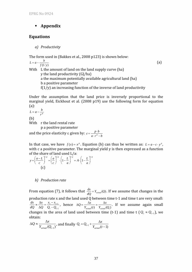
EPRG No 0924
37
Appendix Equations
a) Productivity The form used in (Bakkes et al., 2008 p123) is shown below: L = a −
bf (1 / y)
ith
(a)
W L the amount of land on the land supply curve (ha) (GJ/ha) y the land productivity
a the maximum potentially available agricultural land (ha) b a positive parameter f n n o
(1/y) an increasing fu ctio of the inverse of land pr ductivity Under the assumption that the land price is inversely proportional to the marginal(a):
−b
yield, Eickhout et al. (2008 p19) use the following form for equation
L = ar p
(b) With r the land rental rate p a positive parameter nd the price elasticity ε given by: a p ⋅bε =
a ⋅ r p − b
In that case, we have f (x) = x p . Equation (b) can thus be written as: L = a − c ⋅ y p , with c a positive parameter. The marginal yield y is then expressed as a function of the share of land used L/a:
y =a − L
c⎛ ⎝ ⎜
⎞ ⎠ ⎟
1/ p
=ac
⎛ ⎝ ⎜
⎞ ⎠ ⎟
1/ p
1−⋅La
⎛ ⎝
⎞ ⎠ ⎟ = A L
⎜ 1/ p
⋅ 1−a
⎛ ⎞ ⎝ ⎜
⎠ ⎟ 1/ p
(c)
b) Production rate From equation (7), it follows that dx
dQ= Yactual (Q) . If we assume that changes in the
production rate x and the land used Q between time t‐1 and time t are very small: dxdQ
≈ΔxΔQ
=xt − xt−1
Qt − Qt−1, hence ΔQ =
ΔxYactual (t)
=Δx
Yactual (Qt ). If we assume again small
changes in the area of land used between time (t‐1) and time t (Qt ≈ Q ), we obtain: Δ
t−1
Q ≈Δx
Yactual (Qt−1 ) , and finally Qt = Qt−1 +
ΔxYactual (t −1)

EPRG No 0924
38
Parameters Initial minimum yield
a) Corn yield occurring in U.S. marginally suitable land
Average yal lield a(margin nd)
Minimum y rage yield (very suitable land) ield divided by ave Estimated minimum yield
(marginal land) Y(mS)* Y (m **S) Ymin (VS) ( YVS) / Y(mS) *Ym )/ Y (VS) in(VS ton/1000ha GJ/ha No unit G J/hal 1350 23 0.54 12.4 i 2051 35 0.66 23.1 h 2824 48 0.53 25.4 m 1218 21 0.23 4.8 xi 2064 35 0.55 19.3 xh 2841 48 0.39 18.7 xm 1286 22 0.17 3.7 *(IIASA, 2002) ** Results obtained with heating value of corn of 17 GJ/ton
b) Sugar cane yield occurring in Brazilian marginally suitable land
Aver(marg
age yinal l
ield and)
Minimum y rage yield (very suitable land) ield divided by ave Estimated minimum yield
(marginal land) Y(mS)* Y (mS)** Ymin (VS) (VS) / Y Y(mS) *Ym )/ Y (VS) in(VS ton/1000ha GJ/ha No unit GJ/ha l 2726 47.43 0.88 41.9 i 3872 67.37 0.77 52.2 h 5101 88.76 0.86 76.5 m 2734 47.57 0.86 41.0 xi 3872 67.37 0.61 41.2 xh 5093 88.62 0.59 52.7 xm 2734 47.57 0.59 28.3 *(IIASA, 2002) ** Results obtained with heating value of sugar cane of 17.4 GJ/ton