Embed Size (px)
Citation preview

Citation: Guillevic, P., Göttsche, F., Nickeson, J., Hulley, G., Ghent, D., Yu, Y., Trigo, I., Hook, S., Sobrino, J.A., Remedios, J., Román, M. & Camacho, F. (2017). Land Surface Temperature Product Validation Best Practice Protocol. Version 1.0. In P. Guillevic, F. Göttsche, J. Nickeson & M. Román (Eds.), Best Practice for Satellite-Derived Land Product Validation (p. 60): Land Product Validation Subgroup (WGCV/CEOS), doi:10.5067/doc/ceoswgcv/lpv/lst.001
Committee on Earth Observation Satellites
Working Group on Calibration and Validation
Land Product Validation Subgroup
Land Surface Temperature Product Validation Best Practice Protocol
Version 1.0 - October, 2017
Editors: Pierre Guillevic, Frank Göttsche, Jaime Nickeson, Miguel Román
Authors: Pierre Guillevic, Frank Göttsche, Jaime Nickeson, Glynn Hulley, Darren Ghent, Yunyue Yu, Isabel Trigo, Simon Hook, José A. Sobrino, John Remedios, Miguel Román and Fernando Camacho

2
List of Revisions
Version Revision Date Author V0.0 Initial draft for internal review April 2017 Guillevic V1.0 CEOS LPV peer-reviewed version October 2017 Guillevic et al.

3
Editor’s Note
The editors of this document express the views of the land surface temperature (LST) and emissivity
focus area of the Committee on Earth Observation Satellites (CEOS) Working Group on Calibration and
Validation (WGCV) Land Product Validation (LPV) subgroup. This focus area provides those involved in
the production and validation satellite-based LST products with a forum for documenting accepted best
practices in an open and transparent manner. The LST product validation best practice protocol document
(V1.0) presented here has undergone scientific review by remote sensing experts from across the world. All
comments and suggestions have been carefully considered to formulate this consensus document, which is
freely available on the LPV subgroup web site (http://lpvs.gsfc.nasa.gov/). Furthermore, a list of
recommendations arising from the findings in this document is also provided at the LPV webpage. It is
expected that this best practice protocol will be a living document and that recommendations within will
undergo regular revisions based on community feedback and advancement in the science of LST.
We welcome all interested experts to participate in improving this document and we invite the broader
community to use it for their research and applications related to LST products derived from satellite
imagery. All contributors will be recognized as such in the document and on the CEOS WGCV LPV web
site.
Sincerely,
The Editors:
Pierre Guillevic, University of Maryland, NASA Goddard Space Flight Center
Frank Göttsche, Karlsruhe Institute of Technology (KIT)
Jaime Nickeson, SSAI, NASA Goddard Space Flight Center
Miguel Román, NASA Goddard Space Flight Center (LPV Chair)
Chairpersons of the CEOS WGCV Land Product Validation Group:
Miguel Román, NASA Goddard Space Flight Center (LPV Chair)
Fernando Camacho, EOLAB (LPV Vice-Chair)

4
Table of Contents SUMMARY 8
1 INTRODUCTION 111.1 Importance of Land Surface Temperature 111.2 The UNFCCC and the Global Climate Observing System 121.3 The Role of CEOS WGCV 121.4 LST Requirements 141.5 Rationale for Requirements for Climate Applications 141.6 Goal of this Document 15
2 DEFINITIONS 152.1 Definition of Land Surface Temperature 152.2 Definitions of Associated Physical Parameters 15
2.2.1 Black body 152.2.2 Surface emissivity 152.2.3 Brightness temperature 15
2.3 Definition of Spatial and Geometrical Aspects 162.3.1 Elementary Sampling Unit (ESU) 162.3.2 Local Horizontal Datum 162.3.3 Projected Instantaneous Field of View (PIFOV) of Measurement 162.3.4 Effective Projected Instantaneous Field of View (EPIFOV) of Measurement 162.3.5 Satellite Measurement Geolocation Uncertainty 162.3.6 Mapping Unit 17
2.4 Definition of Validation Metrics 17
3 GENERAL CONSIDERATIONS FOR SATELLITE LST PRODUCTS 183.1 Radiance components and LST retrieval 183.2 Current satellite-based LST products 18
3.2.1 MODIS 193.2.1.1 Split-window-based algorithm 193.2.1.2 Temperature Emissivity Separation (TES) algorithm 19
3.2.2 SEVIRI 203.2.3 VIIRS 203.2.4 NOAA Enterprise LST algorithm 213.2.5 SLSTR 22
3.3 GENERAL CONSIDERATIONS FOR IN SITU REFERENCES 233.3.1 Existing in situ networks of LST reference measurements 23
3.3.1.1 Fluxnet network 243.3.1.2 NASA JPL sites 253.3.1.3 SURFRAD network 253.3.1.4 NOAA USCRN network 27

5
3.3.1.5 GCU stations 283.3.1.6 KIT stations 29
3.3.2 Uncertainties Related to Input Data 313.3.2.1 Radiometric calibration 323.3.2.2 Surface emissivity 333.3.2.3 Atmospheric downwelling radiance 33
3.3.3 Geometric Considerations 343.4 Reference LST Estimates 35
3.4.1 The Elementary Sampling Unit (ESU) Mapping Unit 353.4.2 ESU LST Uncertainty 353.4.3 Upscaling of Reference LST Estimates 363.4.4 Temporal sampling 36
4 GENERAL STRATEGY FOR VALIDATION OF LST PRODUCTS 374.1 CEOS Validation Stages 374.2 Status of Current Validation Capacity and methods 37
4.2.1 Methods 374.2.1.1 Ground-based validation 384.2.1.2 Satellite product Inter-Comparison 394.2.1.3 Radiance-based Validation 404.2.1.4 Time series Inter-Comparisons 42
4.3 Validation Strategy 434.3.1 Direct validation on a global basis representative of surface types and seasonal 434.3.2 Quantify the representative LST accuracy estimate over areas or time periods without reference datasets 434.3.3 Quantify the long term (inter-annual) stability in LST products 44
4.4 Reporting Results of LST product Validation 454.4.1 Validation metrics 454.4.2 Reporting validation results 45
5 CONCLUSIONS 46
6 APPENDIX A: EXAMPLE OF UPSCALING METHOD USING HIGH RESOLUTION VEGETATION DATA TO DRIVE A LAND SURFACE MODEL 48
7 REFERENCES 51

6
List of Figures Figure 1. Location of ground observational networks currently used to validate standard LST products derived
from US and European spaceborne instruments.
Figure 2: Relative spectral response of the SLSTR, MODIS and VIIRS thermal bands around 11 µm and 12 µm. Data are from the MODIS Characterization Support Team at NASA Goddard Space Flight Center for MODIS, from NOAA National Calibration Center for VIIRS and from ESA Sentinels Scientific Data Hub for SLSTR.
Figure 3. Pictures of four different field stations: instrumented JPL’s buoys over Lake Tahoe (upper left), stations from NOAA’s SURFRAD network - Bondville, IL (upper right), Desert Rock, NV (bottom left) and Fort Peck, MT (bottom right).
Figure 4. (left) Locations of the U.S. CRN stations over the USA. (Right) Photography of the station located in Riley, OR.
Figure 5. Schematic description of a U.S. Climate reference Network station. Each station has the same design. Courtesy of the NCDC’s graphic team.
Figure 6. Test sites locations (up) and plots (down) of the fixed stations. From left to right: Doñana (Cortes, Fuente Duque and Juncabalejo), Cabo de Gata (Balsa Blanca) and Barrax (El Cruce and Las Tiesas) test sites. From Sobrino and Skokovic (2016).
Figure 7. (a) Locations of the KIT’s validation stations. African stations at (b) Dahra, Senegal, (c) Gobabeb, Namibia and (d) Farm Heimat, Namibia (Kalahari rainy season).
Figure 8. Representation of scaling and directional effects.
Figure 9. VIIRS (left) and MODIS (right) LST products versus ground-based LST measurements at the KIT stations in Gobabeb, Namibia. Due to an overestimation of surface emissivity values used in the algorithms, both VIIRS and MODIS products significantly underestimate the LST of the Namibian desert by more than 4 K on average (From Guillevic et al., 2014). The figure illustrates the critical needs for ground-based reference: two different satellite LST products can be in very good agreement since they use a similar algorithm, however they may differ considerably from the corresponding ground-based reference measurements.
Figure 10. Differences between VIIRS and MODIS (MYD11) LST products observed over the western USA on two different dates associated with different atmospheric conditions: hot and wet in August 11, 2012, cool and dry in October 14, 2012. The white areas over land are regions where good-quality retrievals were not available (clouds, etc.) (From Guillevic et al., 2014).
Figure 11. An example of the R-based validation method applied to the MODIS Aqua MOD11 and MOD21 LST products over six pseudo-invariant sand dune sites using all data during 2003-2005. Since very few in situ measurements of LST exist over arid regions, the R-based method is the only objective means to validate satellite LST products over these types of land surfaces over long time periods. In this case the R-based method exposed a 3-5 K cold bias in the MYD11 LST product due to overestimation of desert emissivity values.
Figure 12. MODIS LST uncertainty distribution derived from TEUsim plotted versus Total Column Water (TCW) and simulated LST for graybody surfaces (left) and barren surface (right).
Figure A-1. Spatial variability of land cover type and vegetation density before and after harvest around two NOAA’s stations part of the SURFRAD and US CRN network near Bondville, IL.

7
Figure A.2. VIIRS LST product vs. ground-based LST measurements at 8 validation sites (7 SURFRAD stations and JPL buoys at lake Tahoe) representative of various land surface types over the contiguous United States. Results for vegetation sites are with and without scaling (From Guillevic et al., 2014).
List of Tables Table 1. LST product requirements for climate related studies.
Table 2. In-situ LST networks.
Table 3. Examples of FLUXNET/AmeriFlux stations including site geolocation, primary surface type and available period of time for each dataset
Table 4. List of JPL inland water sites including geolocation, elevation, surface emissivity and basic description of the surface type at station location and around the station within moderate resolution satellite footprints.
Table 5. List of validation sites including geolocation, elevation, broadband emissivity and basic description of the surface type at station location and around the station within moderate resolution satellite footprints.
Table 6. List of KIT validation stations including geolocation, elevation, surface emissivity (MSG/SEVIRI
channel 10.8 µm) and basic description of the surface type at station location and around the station within moderate resolution satellite footprints.
Table 7. Example of uncertainty ranges of parameters for in ground-based LST uncertainty estimates (from Sobrino and Skokovic, 2016). Values may depend on specific experimental design.
Table 8. The CEOS WGCV Land Product Validation Stages.
Table 9. Common practice and recommended good practice.

8
SUMMARY The Global Climate Observing System (GCOS) has specified the need to systematically generate and
validate Land Surface Temperature (LST) products. This document provides recommendations on good
practices for the validation of LST products. Internationally accepted definitions of LST, emissivity and
associated quantities are provided to ensure the compatibility across products and reference data sets. A
survey of current validation capabilities indicates that progress is being made in terms of up-scaling and in
situ measurement methods, but there is insufficient standardization with respect to performing and
reporting statistically robust comparisons.
Four LST validation approaches are identified: (1) Ground-based validation, which involves
comparisons with LST obtained from ground-based radiance measurements; (2) Scene-based inter-
comparison of current satellite LST products with a heritage LST products; (3) Radiance-based validation,
which is based on radiative transfer calculations for known atmospheric profiles and land surface emissivity;
(4) Time series comparisons, which are particularly useful for detecting problems that can occur during an
instrument’s life, e.g. calibration drift or unrealistic outliers due to undetected clouds. Finally, the need for
an open access facility for performing LST product validation as well as accessing reference LST datasets is
identified.

9
List of Acronyms and Nomenclature
AATSR Advanced Along-Track Scanning Radiometer
ATBD Algorithm Theoretical Basis Document
AVHRR Advanced Very High Resolution Radiometer
BT Brightness Temperature
CEOS Committee on Earth Observation Satellites
CRN Climate Reference Network
E Surface emissivity
ECMWF European Center for Medium range Weather Forecasting
ECV Essential Climate Variable (GCOS)
EPIFOV Effective Projected Instantaneous Field of View
ESA European Space Agency
ESU Elementary Sampling Unit
FLUXNET Global network of flux tower sites
FOV Field of View
GCM General Circulation Model
GCOS Global Climate Observing System
GCU Global Change Unit (at the University of Valencia)
GMAO Global Modeling and Assimilation Office
IPCC Inter-governmental Panel on Climate Change
ISO International Organization for Standardization
KIT Karlsruhe Institute of Technology
LAI Leaf Area Index
LSA-SAF Land Surface Analysis – Satellite Application Facility
Landsat ETM+ Landsat Enhanced Thematic Mapper +
Landsat TM Landsat Thematic Mapper
LPV Land Product Validation (sub-group of CEOS WGCV)
LST Land Surface Temperature
LTER Long Term Ecological Research Network
MAD Median Absolute Deviation
ME Median Error
MODAPS MODIS Adaptive Processing System
MODIS Moderate Resolution Imaging Spectroradiometer (NASA)
NASA National Aeronautics and Space Administration (USA)
NCEP National Centers for Environmental Prediction
NEON National Environmental Observation Network (USA)
NIST National Institute of Standards and Technology (USA)
NPL National Physical Laboratory (UK)
OLIVE On-Line Validation Exercise

10
ORNL Oak Ridge National Laboratory (USA)
PIFOV Ground Projected Instantaneous Field of View
PTB Physikalisch-Technische Bundesanstalt (Germany)
QA Quality Assessment
RMSE Root Mean Square Error
SLSTR Sea and Land Surface Temperature Radiometer
STD Standard Deviation
SURFRAD Network of surface radiation measurement sites
TIR Thermal Infrared
TOA Top of Atmosphere
UNFCCC United Nations Framework Convention on Climate Change
WGCV Working Group on Calibration and Validation (CEOS)
WMO World Meteorological Organization

11
1 INTRODUCTION This section describes the international framework that has motivated this document, describes the
associated Land Surface Temperature (LST) requirements and summarizes the goals of the presented
validation protocol.
1.1 Importance of Land Surface Temperature
Energy and water exchanges at the land surface – atmosphere interface have a major influence on the
Earth's weather and environment. LST is a fundamental variable in the physics of land surface processes
from local to global scales and is closely linked to radiative, latent and sensible heat fluxes at the surface-
atmosphere interface. Thus, understanding and monitoring the dynamics of LST and its links to human
induced changes is critical for modeling and predicting environmental changes due to climate variability as
well as for many other applications such as geology, hydrology and vegetation monitoring. From a climate
perspective, LST is important for evaluating land surface and land-atmosphere exchange processes,
constraining surface energy budgets and model parameters, and providing observations of surface
temperature change both globally and in key regions. LST has been used for monitoring climate warming
trends over Greenland (Hall et al., 2012), inland water bodies (Schneider and Hook, 2010), and more
recently in urban areas (Malakar and Hulley, 2016). Numerical models ranging from local to global scales
represent and predict effects of surface fluxes. LST versatility has been previously demonstrated in a wide
variety of Earth science research over the past two decades, including reducing and understanding systematic
biases in land surface models (Zhou et al., 2003; Zheng et al., 2012; Trigo et al., 2015; Orth et al., 2017),
filling gaps where few in situ measurements of surface air temperatures exist (e.g. over Africa). Human
health studies include estimating urban heat island effects (Dousset and Gourmelon, 2003; Sobrino et al.,
2013; Luvall et al., 2015), spatial mapping of heat waves in urban and rural regions (Dousset et al., 2011;
Krehbiel and Henebry, 2016), and epidemiological studies about the exposure risk to Lyme and tick-borne
encephalitis (Randolph et al., 2000; Neteler, 2005). LST has also been used for predicting the most
favorable areas for vector-borne diseases, e.g. from Asian tiger mosquito outbreaks in Europe (Neteler et al.,
2011). In the agricultural sector, LST has been used to detect and characterize droughts, plant stress and
water consumptive use (Kogan 1995, 1997; Singh et al., 2003; Fisher et al., 2008; Rojas et al., 2011;
Anderson et al., 2011a; Hain et al., 2011; Gallego-Elvira et al., 2013; Mu et al., 2013; Anderson et al.,
2016a, 2016b and Semmens et al., 2016), surface hydrology and evapotranspiration retrieval (Sandholt et
al., 2002; Nishida et al., 2003; Cleugh et al., 2007; Kalma et al., 2008; Anderson et al., 1997, 2011b, 2012;
Allen et al., 2007). From LST daily time series, indices for mapping heat requirements for grapevine varieties
can be calculated to characterize potential growing regions for viticulture (Zorer et al., 2013), in addition to
being able to predict crop ripening (Hall and Jones, 2010; Jones et al., 2010) and insect infestations (Pasotti
et al., 2006; da Silva et al, 2015). Other direct practical applications of LST concern land-cover change
analyses (Lambin and Ehrlich, 1997; Barbosa et al., 1998), the derivation of snow cover and wetness maps
(Basist et al., 1998), the detection of fundamental changes in land-surface energy partioning (Mildrexler et
al., 2007), land cover classification (Roy 1997), thermal inertia (Sobrino and El Kharraz, 1999) and cloud

12
detection (Jedlovec et al., 2008; Stöckli, 2013). More than 30 thermal infrared applications were identified
in Sobrino et al. (2016). Furthermore, spectral emissivity, an important variable that is used to derive LST
and is often retrieved together with the LST, can be used to monitor and assess melt zones on glaciers, and
in detecting land cover change and degradation (Hulley et al., 2014).
1.2 The UNFCCC and the Global Climate Observing System
Worldwide systematic observation of the climate system is required for advancing scientific knowledge
on changes to our climate. The United Nations Framework Convention on Climate Change (UNFCCC)
calls on the Parties to promote and cooperate in this systematic observation of the climate system, including
support of existing international programs and networks, as indicated in Articles 4.1(g) and 5 of the
Convention. A key dimension for the implementation of those Articles has been the cooperation with the
Global Climate Observing System (GCOS), a joint undertaking of the World Meteorological Organization
(WMO), the Intergovernmental Oceanographic Commission (IOC) of the United Nations Educational
Scientific and Cultural Organization (UNESCO), the United Nations Environment Programme (UNEP)
and the International Council for Science (ICSU) with its secretariat hosted by the WMO, reinforced by
decisions taken at various Conferences of the Parties. The signatories of the UNFCCC have thus adopted
the GCOS as the organizing body for climate observations expressed through its Implementation Plans
(GCOS-82, GCOS-200). These Implementation Plans establish the requirements for the systematic
monitoring of a suite of Essential Climate Variables (ECV) globally. Land Surface Temperature (LST) is one
of the terrestrial ECVs recognized by GCOS (GCOS-200).
1.3 The Role of CEOS WGCV
LST can be measured in situ and from remote observations. While it is routinely measured at a
number of research sites, the measurement network is sparse in many regions of the world. Figure 1 presents
different networks or individual sites currently used to validate LST standard products derived from US and
European instruments (as of September 2017). This dataset should be maintained and ideally expanded to
become much more representative of the diversity of ecosystem and climatic conditions.

13
Figure 1. Location of ground observational networks currently used to validate standard LST products derived from
US and European spaceborne instruments.
The process of improving both space-based observations and in situ networks is embodied in the
GCOS Implementation Plans and the accompanying Satellite Supplements (GCOS-200). The Committee
on Earth Observation Satellites (CEOS) Working Group on Calibration and Validation (WGCV), and in
particular its subgroup on Land Product Validation (LPV), plays a key coordination role and lends the
expertise required to address actions related to the validation of LST measurements as follows:
- In-situ LST is usually estimated from up- and downwelling thermal infrared (TIR) radiance
measurements near the surface. The radiances are either obtained with a set of radiometers (directional
measurements) or pyrgeometers (hemispherical measurements). A number of observational sites
dedicated to surface climate, ecological, or agricultural research and applications provide in-situ LST on
a routine basis. CEOS WGCV plays a coordinating role in this work. Benchmarking and consistency
checking are required for the global archive of LST observations.
- The setting up and maintenance of reference sites to address the inadequate or missing reference
network need to be undertaken. Building on existing networks - such as the National Oceanic and
Atmospheric Administration (NOAA) Surface Radiation (SURFRAD) and US Climate Reference
Network (CRN) networks, the Land Surface Analysis – Satellite Application Facility (LSA–SAF)
permanent validation sites for EUMETSAT satellite products, NASA’s Jet Propulsion Laboratory (JPL)
validation sites - is the most promising way to improve this situation.
- Benchmarking and comparison of satellite-derived LST products is essential to resolve differences
between products and to ensure their consistency in terms of accuracy and reliability. The CEOS
WGCV is leading this activity in collaboration with GCOS and TOPC, exploiting in situ observations
from designated reference sites and building on the validation activities currently being undertaken by
the space agencies and associated research programs (GCOS-200, p. 203).
CEOS considers these roles important to achieving validated global LST products, but at the same

14
time, recognizes current limitations in both resources and knowledge within both CEOS and the
international expert community. This good practice document includes recommendations from CEOS that,
if followed, should serve to remove many of the current limitations.
1.4 LST Requirements
The user-driven baseline requirements for satellite-derived LST climate data records (Table 1) used in
climate studies have been determined by the CEOS WGCV Land Product Validation subgroup and the
International Land Surface Temperature and Emissivity Working Group (http://ilste-wg.org). The values in
Table 1 are the thresholds that represent the minimum requirements for LST data to be useful for climate
applications (GCOS-200); target values are indicated where understood (i.e. length of record requirements
are difficult to quantify). In this protocol, we will focus primarily on LST datasets generated from infrared
instruments, which only allow LST retrievals under clear sky conditions. Although LST can also be
estimated from passive micro-wave sensors under both clear and cloudy situations (e.g., Jimenez et al., 2017),
micro-wave based LST are not only beyond the spatial resolution threshold (Table 1), as their maturity has
not yet reached that of infrared based products (e.g., Ermida et al., 2017).
Table 1. LST product requirements for climate related studies
Requirement Threshold Target (breakthrough) Horizontal resolution 5 km (i.e. 0.05°) ≤ 1 km Temporal resolution ≤ day/night (12h) 3-hourly Uncertainty 1 K 0.1 K Precision 1 K 0.1 K Stability ≤ 0.3 K per decade ≤ 0.1 K per decade Length of record 20 years >30 years
It should be noted that LST product requirements strongly depend on the target application. For
example, agricultural applications such as crop condition monitoring or irrigation management, require
higher spatial resolutions (~100 m or higher).
1.5 Rationale for Requirements for Climate Applications
LST is the intrinsic quantity required by the climate user community. However, it is recommended that
emissivity values are reported as part of a climate quality LST product. Likewise, although sensor and
channel specific, it is recommended that land surface brightness temperature is also reported as part of the
LST climate quality product to allow producers and users to derive LST data sets with alternative retrieval
methods.
Although there are issues with respect to satellite radiometer stability and cloud masks reliability, the
specifications of existing (and planned) space-based instruments meet or largely exceed the spatial and
temporal sampling requirements of General Circulation Models (GCM). The higher frequency of
observations today provide us with accurate and stable products that are able to support a host of other
downstream applications. Even in the context of climate applications, high spatial resolution products
support high-resolution regional models, as well as global models, and allows for examination of the
sensitivity of land-surface parameterizations with respect to surface heterogeneity, and to capture rapid

15
changes in vegetation phenology, surface hydrology, and anthropogenic effects.
1.6 Goal of this Document
The goal of this document is to identify and promote good practices for the validation of global satellite
LST products. The document specifically addresses uncertainty assessment against reference datasets. The
latter should be traceable to in situ measurements of known accuracy, and the assessment augmented with
metrics of precision derived from ensembles of products themselves. The development of validation
protocols also addresses the GCOS Action Items.
2 DEFINITIONS This section provides the necessary definitions relevant to global LST validation.
2.1 Definition of Land Surface Temperature
LST is a kinetic quantity, independent of wavelength, that represents the thermodynamic temperature
of the skin layer of a given surface, i.e. a measure of how hot or cold the surface of the Earth would feel to
the touch. For ground-based, airborne, and spaceborne remote sensing instruments LST is the aggregated
radiometric surface temperature, i.e. based on a measure of radiance (Norman and Becker, 1995), of the
ensemble of components within the sensor field of view. LST is sometimes referred to in the literature as
(directional) radiometric temperature or skin temperature. The unit of LST is Kelvin [K]; Degree Celsius
[°C] is also commonly used. When derived from radiometric measurements of ground-based, airborne, and
space-borne remote sensing instruments, LST is the aggregated radiometric surface temperature of the
ensemble of components within the sensor field of view. This definition was adopted across various
international groups (CEOS WGCV, GCOS, ESA GlobTemperature, ILSTE-WG), and was pioneered by
the work of John Norman and François Becker (see Norman and Becker, 1995, for example).
2.2 Definitions of Associated Physical Parameters
2.2.1 Black body
A black body is an idealized physical body that absorbs all incident electromagnetic radiation in the
thermal infrared and does not reflect any. The emissivity of a black body is equal to 1.
2.2.2 Surface emissivity
“Surface emissivity of an isothermal, homogeneous body is defined as the ratio of the actual emitted
radiance to the radiance which would be emitted from a perfectly emitting surface (i.e. ‘blackbody’) at the
same thermodynamic temperature” (Norman and Becker, 1995).
2.2.3 Brightness temperature
“Brightness temperature is a directional temperature obtained by equating the measured radiance with
the integral over wavelength of the Planck's Black Body function times the sensor response. It is the
temperature of a black body that would have the same radiance as the radiance actually observed with the
radiometer. This requires specification of wavelength interval, direction and whether the observation is

16
above the atmosphere from a satellite or immediately above the surface.” (Norman and Becker, 1995)
2.3 Definition of Spatial and Geometrical Aspects
Validation of satellite LST products relies on terminology specific to satellite measurements. This
section reviews the terminology used in this context. The following definitions were adapted from the
Global Leaf Area Index validation best practice document (Fernandes et al., 2014).
2.3.1 Elementary Sampling Unit (ESU)
An Elementary Sampling Unit (ESU) is a contiguous spatial region over which the expected value of
LST can be estimated through in situ measurements. The ESU corresponds to the finest spatial scale of LST
estimates used for reference. ESU size is bounded by an instrument's sampling characteristics and may
involve a number of measurements. Maximum ESU size is determined by the level of within-ESU variability
that can be tolerated by the validation protocol. Within a reference region, the appropriate ESU size varies
with surface conditions, the instrument used, illumination conditions and spatial sampling design. ESU size
should be sufficient to allow repeat visits with negligible uncertainty contributions due to changes in
illumination or geolocation.
2.3.2 Local Horizontal Datum
The local horizontal datum is the plane containing the tangent to the local geoid corresponding to the
center of an ESU or mapping unit. Depending on the survey method over sloped terrain, corrections of LST
estimates for the dependency of observed surface area on slope may be required.
2.3.3 Projected Instantaneous Field of View (PIFOV) of Measurement
The ground projected instantaneous field of view (PIFOV) is the area on the ground corresponding to
the region over which a measurement is performed. For radiometric measurements, this area is defined as
the region where the instrument point spread function, including all processing aspects except for spatial
resampling, exceeds a specified threshold. The majority of imaging scanners including satellite imagers have
PIFOV on flat ground on the order of twice the inter pixel sampling distance. The PIFOV of an in situ
instrument will vary with the height and angular sampling of the instrument.
2.3.4 Effective Projected Instantaneous Field of View (EPIFOV) of Measurement
The effective projected instantaneous field of view (EPIFOV) corresponds to the PIFOV extended by
the impact of spatial resampling. Resampling with smoothing filters (e.g. cubic convolution) will result in an
EPIFOV with a size approximating the PIFOV convolved with the size of the filter spatial support. Non-
linear resampling, such as nearest neighbor, can result in substantial spatial aliasing. Hence, comparisons of
values recorded in different EPIFOVs should include spatial averaging using a filter with a spatial support of
several PIFOVs.
2.3.5 Satellite Measurement Geolocation Uncertainty
Geolocation uncertainty corresponds to the planimetric uncertainty of a satellite measurement located
on the same projection and datum as the ESU or study site reference LST estimates. Geolocation

17
uncertainty is often reported in nominal terms and based on a normal distribution of errors. Acquisition
specific biases are surprisingly frequent and, therefore, geolocation uncertainty should be visually compared
to reference vector layers whenever possible.
2.3.6 Mapping Unit
A mapping unit is the spatial region on the Earth’s surface corresponding to a product value for a
specified temporal extent. Satellite based LST products represent swaths or gridded digital layers in a
specified map projection rather than per nominal EPIFOV location. As such, these products include a
spatial generalization corresponding to the transformation of LST estimate over each EPIFOV to the LST
estimate for the mapping unit. Considering that GCOS requires gridded LST products at a constant spatial
resolution, the CEOS LST validation protocol assumes uncertainties due to this generalization or due to
temporal aggregation, are included in total product uncertainty.
2.4 Definition of Validation Metrics
Validation is the process of assessing, by independent means, the quality of the data products derived
from those system outputs. In general, the result of a measurement is only an approximation or estimate of
the value of the measurand and thus is complete only when accompanied by a statement of the uncertainty
of that estimate. Definitions of validation metrics (uncertainty, bias, precision and completeness) drawn
from experimental statistics that are applicable to LST are from the Joint Committee for Guides in
Metrology (JCGM) guide to the expression of uncertainty in measurement, referred to as GUM-2008
hereafter. The definitions used in this document and reported below are mainly from GUM-2008:
- Error (of measurement) is “the result of a measurement minus a true value of the measurand”. The
true value (of a quantity) is the “value consistent with the definition of a given particular quantity”.
Since a true value cannot be usually determined, in practice a conventional true value is used. The
conventional true value (of a quantity) is the “value attributed to a particular quantity and accepted,
sometimes by convention, as having an uncertainty appropriate for a given purpose”. Traditionally, an
error is viewed as having two components, namely, a random component and a systematic component.
The random error is the “result of a measurement minus the mean that would result from an infinite
number of measurements of the same measurand carried out under repeatability conditions” and the
systematic error is the “mean that would result from an infinite number of measurements of the same
measurand carried out under repeatability conditions minus a true value of the measurand”.
- Uncertainty is a “parameter, associated with the result of a measurement, that characterizes the
dispersion of the values that could reasonably be attributed to the measurand”. Uncertainty includes
bias and precision errors and can be estimated by the Root Mean Square Error (RMSE).
- Accuracy is the degree of “closeness of the agreement between the result of a measurement and a true
value of the measurand”. Commonly, accuracy is represented as a description of systematic errors and a
measure of statistical bias. Bias is the systematic error between LST products and their reference
estimates, i.e. it describes the average deviation from the reference, which is given by the average
difference between the LST product and its reference estimate.
- Precision or repeatability (of results of measurements) is the “closeness of the agreement between the

18
results of successive measurements of the same measurand carried out under the same conditions of
measurement”. Commonly, precision represents the dispersion of product retrievals around their
expected value and can be estimated by the standard deviation (STD) of the difference between
retrieved LSTs and the corresponding reference estimates.
- Completeness is the proportion of valid retrievals over an observation domain.
It should be noted that strong and/or multiple outliers affect the classical metrics described above (i.e.
mean and STD): in such cases using the median in lieu of the mean to estimate systematic error and the
median absolute deviation as a measure of precision is more suitable and should be included in the
validation effort.
3 GENERAL CONSIDERATIONS FOR SATELLITE LST PRODUCTS
3.1 Radiance components and LST retrieval
Under clear sky conditions, the top of atmosphere radiance measured by a spaceborne sensor (𝐿"#$,&)
includes contributions from the surface emission, the atmospheric upwelling radiance (𝐿"'(,&↑ ) and
atmospheric downwelling radiance (𝐿"'(,&↓ ) reflected by the Earth’s surface and attenuated by the
atmosphere (Eq. 1). Retrieval algorithms rely on one or more top-of-atmosphere spectral measurements to
account for atmospheric effects and estimate LST.
L,-.,/ = ε/B/ LST + 1 −ε/ L,9:,/↓ τ/ +L,9:,/↑ (1)
where 𝜀&is the spectral emissivity at wavelength l or representative of a specific (relatively narrow)
domain [l1, l2] centered on wavelength l, 𝐵& 𝑇 is the Planck function describing the radiance of a black
body at temperature T, and 𝜏& is the atmospheric transmittance.
3.2 Current satellite-based LST products
Operational LST products are currently available from a variety of instruments. In this document, we
mainly focused on products that can be used for climate related studies (i.e. following product requirements
described in Table 1). We have selected some of most commonly used operational and standard LST
products to present the different retrieval algorithms that can be used at moderate resolution, and present
the potential sources of uncertainty that have been already discussed in the literature. The selected products
are based on radiometric measurements by the Moderate Resolution Imaging Spectroradiometer (MODIS)
sensor aboard the Terra and Aqua satellites, the Advanced Baseline Imager (ABI) aboard Geostationary
Operational Environmental Satellite (GOES)-R, the Spinning Enhanced Visible & Infrared Imager
(SEVIRI) aboard the Meteosat satellite series, the Sea and Land Surface Temperature Radiometer (SLSTR)
on the Sentinel-3 platform and the Visible Infrared Imaging Radiometer Suite (VIIRS) onboard the S-NPP
satellite.

19
3.2.1 MODIS
3.2.1.1 Split-window-based algorithm
NASA’s operational MODIS LST product based on the split-window approach consists of Level-2
(MOD11_L2) products at the spatial resolution of MODIS, i.e. 927 m at nadir, and gridded Level-3
(MOD11A1, MOD11A2, MOD11B1, MOD11C1, MOD11C2, MOD11C3) products at 1km or 5km
spatial resolution. Satellite overpass times at the equator are around 10:30am/pm (local solar time) for Terra
and 1:30am/pm for Aqua. Along each scan, the MODIS off-nadir scan angle increases to values of up to
65°, which causes the sensor’s spatial resolution to degrade to about 6 km in the along-scan direction. The
generalized split-window algorithm (Wan and Dozier, 1996) is used to derive LST values from brightness
temperature measurements in MODIS band 31 (T31) and band 32 (T32) centered on 11.03 µm and
12.02 µm, respectively (Eq. 2).
𝐿𝑆𝑇 = 𝑏B + 𝑏C + 𝑏D1 − 𝜀𝜀 + 𝑏E
∆𝜀𝜀D
𝑇EC + 𝑇ED2 + 𝑏H + 𝑏I
1 − 𝜀𝜀 + 𝑏J
∆𝜀𝜀D
𝑇EC − 𝑇ED2 (2)
where 𝜀 and ∆𝜀 are the mean and the difference of the emissivity values in bands 31 and 32. The
algorithm coefficients bk (with k = 0 to 6) depend on viewing zenith angle, surface air temperature (Tair) and
atmospheric water vapor content. The coefficients were derived for daytime and nighttime from regression
analysis of radiative transfer simulation data for a comprehensive set of LST values varying from Tair – 16 K
to Tair + 16 K (Wan and Dozier, 1996) accounting for the MODIS spectral response function - see Figure 2.
In the standard LST product, information about surface air temperature and total column water vapor is
taken from the MODIS atmospheric profile product (MOD07) (Wan, 2008). For each surface type, the
spectral emissivity values in band 31 and 32 (Eq. 1) are defined as a combination of green and senescent
components (Snyder et al., 1998).
3.2.1.2 Temperature Emissivity Separation (TES) algorithm
Initially developed for the Advanced Spaceborne Thermal Emission and Reflection Radiometer
(ASTER) sensor on Terra, the Temperature-Emissivity Separation (TES) method (Gillespie et al. 1998) is an
alternative physics-based approach that was adapted for MODIS (Hulley and Hook, 2010) in order to
address emissivity related issues in the heritage MOD11 products resulting in underestimation of LST in
arid regions (Gottsche and Hulley 2012; Hulley and Hook 2009; Malakar and Hulley 2016). The new TES-
based product, termed MOD21 includes both LST and physically retrieved emissivity for the 3 MODIS
thermal bands (29, 31, 32) and is currently being produced as part of the MODIS Collection 6 suite of
products. The TES algorithm uses a radiative transfer model to correct at-sensor radiances to surface
radiances and a statistical emissivity model to separate contributions from surface temperature and
emissivity. The approach requires atmospheric profiles from either satellite sounding or conventional
radiosondes and an emissivity model which is typically based on laboratory and field measurements (Kealy
and Hook, 1993; Matsunaga, 1994). In the TES approach, first the range of relative spectral emissivities (i.e.
the minimum-maximum difference or MMD) is calculated. A calibration curve derived from laboratory data
(Matsunaga, 1994) allows to estimate minimum absolute spectral emissivity from the observed MMD value.
Equation 1 is then used to compute LST and emissivities for the other bands. For MODIS, the ASTER

20
spectral library (Baldridge et al., 2009) is used to derive the calibration curve for three TIR bands: 29
(8.55 µm), 31 (11 µm) and 32 (12 µm): the regression between the minimum emissivities and MMDs
obtained for MODIS is given by Equation 3.
𝜖LMN = 0.985 − 0.7503𝑀𝑀𝐷B.XEDC (3)
where, emin is the minimum emissivity of the three MODIS TIR bands (29, 31 and 32), and MMD is
the difference between the minimum and maximum emissivity values for the given bands. The TES
algorithm is combined with an improved Water Vapor Scaling (WVS; Tonooka, 2005) atmospheric
correction scheme to adjust the retrieval during very warm and humid conditions. Validation results have
shown consistent accuracies at the 1 K level over all land surface types.
3.2.2 SEVIRI
EUMETSAT’s operational LST product for SEVIRI is produced by the Satellite Applications Facility
on Land Surface Analysis (LSA SAF). It is computed every 15 minutes at a spatial resolution of 3 km
(sampling distance at nadir) within the area covered by the Meteosat Second Generation (MSG), i.e.
primarily over Europe, Africa and South America. The retrieval is based on the Generalized Split-Window
algorithm (GSW; Wan and Dozier, 1996; Eq. 2) and uses brightness temperatures measured in channels 9
and 10 centered on 10.8 µm and 12.0 µm, respectively. Emissivity is obtained with the so-called vegetation
cover method (Caselles and Sobrino, 1989; Peres and DaCamara, 2005), where effective channel emissivity
for any given pixel is estimated as a weighted average of channel emissivities of the dominant bare ground
and vegetation types within a scene. The emissivity values for these types are available from look-up tables
(Peres and DaCamara, 2005) determined for International Geosphere-Biosphere Program (IGBP) land cover
classes (Belward, 1996). Actual channel emissivities are then estimated from the fraction of vegetation cover
(FVC) also retrieved by LSA SAF (Garcia-Haro et al., 2005) as five-day composites updated on a daily basis.
Furthermore, the GSW parameters are selected based on forecasts of total column water vapour provided by
the European Centre for Medium-range Weather Forecasts (ECMWF). LSA SAF performed an in-depth
analysis of the various error sources of its GSW algorithm and utilises these to maximize the LST product’s
spatial coverage (Freitas et al., 2010). The LST values are distributed together with realistic estimations of
the respective uncertainties on a pixel-by-pixel basis, allowing users to decide if specific LST data meet their
application requirements. The target accuracy of the SEVIRI LST product is 2 K (Freitas et al., 2010), while
validation against in-situ data showed a general uncertainty of about 1.5 K (Göttsche et al., 2016). The LSA
SAF LST product is described in detail in the corresponding Algorithm Theoretical Basis Document (Trigo
et al., 2009).
3.2.3 VIIRS
Since August 11, 2012, the NOAA VIIRS Environmental Data Record (EDR) has been operationally
produced using a single split window algorithm (Yu et al., 2005). The algorithm uses brightness
temperatures measured in channel M15 (T15) and channel M16 (T16) centered on 10.76 µm and 12.01 µm,
respectively (Eq. 4).
𝐿𝑆𝑇 = 𝑎B +𝑎C𝑇CI +𝑎D 𝑇CI −𝑇CJ +𝑎E 𝑠𝑒𝑐𝜃^ − 1 +𝑎H 𝑇CI −𝑇CJ D (4)

21
where ak (with k = 0 to 4) are the algorithm coefficients and 𝜃^is the sensor zenith angle. Daytime and
nighttime sets of coefficients were derived for 17 different surface types from regression analysis of
MODTRAN radiative transfer simulations for globally representative atmospheric and surface conditions
(VIIRS LST Algorithm Theoretical Basis Document (ATBD), 2011). The International Geosphere-
Biosphere Programme (IGBP) global classification map is used to identify the surface type associated with
each pixel. The algorithm regression coefficients were generated from an ensemble of MODTRAN radiative
transfer simulations using a comprehensive set of geophysical parameters (VIIRS LST ATBD, NOAA 2011).
Surface temperatures and coherent atmospheric temperature and water vapor profiles were derived from
National Center for Environmental Prediction (NCEP) global simulations at 2.5° x 2.5° spatial resolution.
LST values were sampled from 196 K to 327 K. Distribution of band-averaged spectral emissivity values for
each surface type (Eq. 1) were derived from the MOSART database (VIIRS LST ATBD, NOAA, 2011).
These were used to produce a total of 268,128 samples representing 12 days and nights (one day and night
per month) over a global grid, and provided an ensemble of training data covering global, diurnal and
seasonal features (VIIRS LST ATBD, 2011). The spatial resolution of VIIRS raw radiometric measurements
at moderate resolution is around 750 m at nadir and around 1.5 km at the edge of the swath. VIIRS
detectors are rectangular, with the smaller dimension projecting along the scan. At nadir, three detector
footprints are aggregated to form a single VIIRS pixel. Moving along the scan away from nadir, the detector
footprints become larger both along track and along scan, due to geometric effects and the curvature of the
Earth (Wolfe et al., 2013). The pixel aggregation scheme is changed from 3 to 2 detectors at a scan angle of
around 32°, and from 2 to 1 detector at around 48°, which provides a more uniform pixel size over the
scan. The bias and precision requirements specified by NOAA’s Joint Polar Satellite System (JPSS) program
for the VIIRS LST EDR are 1.5 K and 2.5 K, respectively, for clear conditions.
In line with production of the new MOD21 LST&E product, NASA is currently in the processing of
producing an equivalent TES-based product for VIIRS, termed VNP21. The VIIRS Land Surface
Temperature and Emissivity (LST&E) algorithm and data products (VNP21) in Collection 1 (C1) are being
developed synergistically with the MODIS Collection 6 (C6) LST&E algorithms and data products
(MOD21) using the same algorithmic approach and input atmospheric products (Islam et al., 2016; Malakar
and Hulley, 2016).
3.2.4 NOAA Enterprise LST algorithm
NOAA JPSS Land EDR team is developing an enterprise LST algorithm that will be used for both the
JPSS and GOES-R satellite missions. The enterprise algorithm is based on the split-window approach, using
spectral measurements at channels centered on 11 and 12 µm, respectively, and spectral emissivity data (Eq.
5).
𝐿𝑆𝑇 = 𝐶B +𝐶C𝑇CC +𝐶D 𝑇CC −𝑇CD +𝐶Eε +𝐶Hε 𝑇CC −𝑇CD + 𝐶I∆𝜀 (5)
where Ci, i=0 to 5, are the algorithm coefficients; T11 and T12 are the brightness temperatures measured
at the split-window channels (i.e. 11 µm and 12 µm), respectively; ε and ∆𝜀 are the mean emissivity and the
spectral emissivity difference, respectively. Note that the different coefficients set {Ci} are estimated for
daytime and nighttime, and for different atmospheric water vapor conditions. Coefficients are calculated for

22
the JPSS satellite sensor (i.e. VIIRS) and for the GOES-R sensor (i.e. Advanced Baseline Imager, ABI)
accounting for differences in the sensor spectral response function. The split window channels are bands
M31 and M32 for VIIRS, and bands M15 and M16 for ABI.
3.2.5 SLSTR
ESA’s Sentinel-3A SLSTR instrument, launched in February 2016, provides MODIS/VIIRS-like data
(Fig. 2), with a 10am overpass. The SLSTR algorithm (Eq. 6) is an evolution of the LST algorithm developed
for the Advanced Along Track Radiometer (AATSR), aboard ENVISAT, by Prata (2002).
𝐿𝑆𝑇 = 𝑎`,M,a + 𝑏 ,M 𝑇CC − 𝑇CD N + 𝑏 ,M + 𝑐 ,M 𝑇CD
with 𝑛 = 1/cos ghL
, 𝑎`,M,a = 𝑑 𝑠𝑒𝑐𝜃^ − 1 𝑝𝑤 + 𝑎^,M𝑓 + 𝑎",M 1 − 𝑓 ,
𝑏 ,M = 𝑏^,M𝑓 + 𝑏",M 1 − 𝑓 and 𝑐 ,M = 𝑐^,M𝑓 + 𝑐",M 1 − 𝑓
(6)
where 𝑇CC and 𝑇CD are the brightness temperatures from the SLSTR 11 µm and 12 µm bands
respectively, 𝜃^ is the satellite view zenith angle, 𝑓 is the vegetation fraction, 𝑤 is the atmospheric water
content (in cm) and 𝑖 corresponds to the surface type or biome from the Globcover classification. 𝑎^,M, 𝑎",M, 𝑏^,M, 𝑏",M, 𝑐^,M and 𝑐",Mrepresent the algorithm regression coefficients derived for each of the 22 biomes of
Globcover (𝑖) calculated for a vegetation cover fraction of 100% (𝑣) and for a bare soil (𝑠). Two sets of
coefficients are derived for daytime and nighttime observations accounting for the SLSTR spectral response
functions (Figure 2). 𝑑 and 𝑚 are two empirical parameters. A full description of the retrieval algorithm can
be found in the SLSTR Algorithm Theoretical Basis Document (ATBD) for Land Surface Temperature
(Remedios, 2012).
Figure 2: Relative spectral response of the SLSTR, MODIS and VIIRS thermal bands around 11 µm and 12 µm. Data are from the MODIS Characterization Support Team at NASA Goddard Space Flight Center for MODIS, from NOAA National Calibration Center for VIIRS and from ESA Sentinels Scientific Data Hub for SLSTR.

23
3.3 GENERAL CONSIDERATIONS FOR IN SITU REFERENCES
From in situ narrow band measurements of surface-leaving radiance 𝐿pqrsNt,& and downwelling
radiance from the sky 𝐿"'(,&↓ ground-based LST (𝐿𝑆𝑇pqrsNt) is retrieved using Planck’s law (Guillevic et al.,
2014; Göttsche et al., 2016) (Eq. 7).
𝐿𝑆𝑇pqrsNt = 𝐵&uC 1𝜀&
𝐿pqrsNt,& − 1 − 𝜀& 𝐿"'(,&↓ (7)
where 𝜀&is the spectral emissivity at wavelength l or representative of a specific (relatively narrow)
domain [l1, l2] centered on wavelength l, 𝐵& 𝑇 is the Planck function describing the radiance of a black
body at temperature T.
In contrast, from broadband radiance measurements 𝐿pqrsNt and 𝐿"'(↓ , 𝐿𝑆𝑇pqrsNt is retrieved using
Stefan-Boltzmann’s law (Eq. 8) (Wang and Liang, 2009):
𝐿𝑆𝑇pqrsNt = 1𝜀σ 𝐿pqrsNt − (1 − 𝜀)𝐿"'(↓
C/H
(8)
where 𝜀 is the broadband emissivity and 𝜎 the Stefan-Boltzmann constant (=5.67 10-8 Wm-2K-4).
Broadband emissivity can be retrieved from ‘narrowband’ satellite emissivities (e.g. MODIS) via empirical
relationships (Wang and Liang, 2009). Furthermore, empirical relationships can be obtained to map
emissivities from one satellite sensor to another, e.g. from MODIS to SEVIRI (Peres et al., 2014).
3.3.1 Existing in situ networks of LST reference measurements
Several networks and dedicated validation stations are commonly used to validate current standard and
research LST products, e.g. NOAA’s Surface Radiation (SURFRAD) network, the US Climate Reference
Network (CRN), KIT’s permanent validations stations operated within the framework of EUMETSAT’s
Land Surface Analysis Satellite Application Facility (LSA SAF), the NASA JPL validation sites, the Fluxnet
tower network, and the sites of the Global Change Unit (GCU) of the University of Valencia in Spain.
These existing observational networks (Table 2) include appropriate tower sites with appropriate sensors and
support (e.g. human maintenance, radiometer availability, site accessibility, and power needs) required for
measuring radiation variables to derive LST. A challenge in deriving high quality in-situ LST is to estimate
critical ancillary data, such as surface emissivity and atmospheric profiles if downwelling atmospheric
radiance is not simultaneously measured. Usually, ancillary data are not routinely collected and have to be
obtained from other sources. While surface measurements are too sparse to systematically validate remote
sensing products in a global sense, they are the only means to validate LST products in a classical sense, i.e.
with independent measurements, and they complement scientific efforts aimed at comparing and
benchmarking the various existing LST products. Pursuing and expanding these measurements is essential
to ensure the quality and reliability of current and future products, to provide a step towards more accurate
and consistent LST information for the global landmass and to serve further development of associated
standards. However, the largest networks (i.e. Fluxnet, SURFRAD and US CRN) were not specifically set up
for LST product validation and the stations are frequently located in heterogeneous areas, resulting in
observations that are not representative of spatially coarser satellite observations. For such sites, validation

24
with ground-based LST should be limited to night-time when land surfaces tend to be close to isothermal
(Wang et al., 2008; Guillevic et al., 2014; Martin and Göttsche, 2016).
Table 2. In-situ LST networks.
Name Type Land Cover Citation FLUXNET Hemispherical pyrgeometers All surface types
JPL network Radiometers Water bodies, agricultural field
Hook et al., 2007
SURFRAD Hemispherical pyrgeometers Short vegetation and barren soils in the USA
Augustine et al., 2000, 2005
US CRN Radiometers Short vegetation and barren soils in the USA
Diamond et al., 2013
GCU stations Radiometers Various surface types in Spain
Sobrino and Skokovic, 2016
KIT stations Radiometers Various surface types in Africa and Portugal
Göttsche et al., 2016
Links to all ground-based LST measurement protocols can be found at the LPV sub-group Surface LST&E Focus Area webpage (https://lpvs.gsfc.nasa.gov/LST_home.html).
3.3.1.1 Fluxnet network
The Fluxnet network (Baldocchi et al., 2001) provides continuous observations of ecosystem level
exchanges of CO2, water and energy, and micrometeorological parameters at diurnal, seasonal, and
interannual time scales. The FLUXNET stations operate in climatologically diverse regions and are
representative of various land cover types (Table 3). Over the contiguous United States, the Fluxnet stations
are part of the Ameriflux network and collect measurements of radiative forcing (shortwave and longwave
downwelling and outgoing radiation), surface fluxes (soil heat and convective fluxes), and atmospheric
parameters (air temperature and wind speed). AmeriFlux instruments are meticulously maintained and a
detailed description of the network and a summary of the accuracy assessment of each instrument are
provided by Baldocchi et al. (2001). Upwelling and downwelling thermal infrared radiances measured by
two pyrgeometers (spectral range from around 3.5 to 50.0 µm) can be used to derive ground-based LST
following Equation 7. However, despite the good quality of the collected data, the FLUXNET network has
not been used for satellite-derived LST product validation in a routine manner yet. AmeriFlux data are
archived and distributed by the Oak Ridge National Laboratory (http://ameriflux.ornl.gov/). For each
selected site, the dataset represents 30-minute averages of each parameter.
Table 3. Examples of FLUXNET/AmeriFlux stations including site geolocation, primary surface type and available period of time for each dataset
Site Lat Lon Surface type Period Climate ARM Great Plains, OK 36.606 -97.489 Cropland 2003-2012 Temperate Audubon Ranch, AZ 31.591 -110.509 Grassland 2004-2008 Semi-arid Bondville, IL 40.006 -88.290 Cropland 1997-2007 Temperate Brookings, SD 44.345 -96.836 Grassland 2005-2009 Temperate Chestnut Ridge, TN 35.931 -84.332 Deciduous broadleaf 2006-2013 Temperate Fermi, IL - Agricultural 41.859 -88.223 Cropland 2006-2011 Temperate Fermi, IL - Prairie 41.841 -88.241 Grassland 2005-2011 Temperate

25
Fort Peck, MT 48.308 -105.102 Grassland 2000-2008 Temperate Freeman Ranch, TX - Mesquite 29.950 -97.996 Grassland 2005-2008 Semi-arid Freeman Ranch, TX - Woodland 29.940 -97.990 Woody savannah 2005-2012 Semi-arid Konza, KS 39.082 -96.560 Grassland 2007-2012 Temperate Loblolly Pine, NC 35.803 -76.668 Evergreen needleleaf 2005-2010 Sub-tropical Loblolly Pine Clearcut, NC 35.812 -76.712 Evergreen needleleaf 2005-2009 Sub-tropical Mead, NE - Irrigated maize 41.165 -96.477 Irrigated cropland 2002-2012 Temperate Mead, NE - Irrigated maize-soybean 41.165 -96.470 Irrigated cropland 2002-2012 Temperate Mead, NE - Rainfed maize-soybean 41.180 -96.440 Rainfed cropland 2002-2012 Temperate Missouri Ozark, MO 38.744 -92.200 Deciduous broadleaf 2005-2013 Temperate Santa Rita Mesquite, AZ 31.821 -110.866 Woody savannah 2004-2013 Semi-arid Tonzi Ranch, CA 38.432 -120.966 Woody savannah 2002-2012 Semi-arid Vaira Ranch, CA 38.413 -120.951 Grassland 2001-2012 Semi-arid Walker Branch, TN 35.959 -84.287 Deciduous broadleaf 1995-2006 Temperate
3.3.1.2 NASA JPL sites
NASA’s Jet Propulsion Laboratory (JPL) has been maintaining continuous LST monitoring stations on
Lake Tahoe, CA/NV, a 35 km long and 15 km wide lake on the California – Nevada border since 1999 and
on the Salton Sea, CA, an inland saline lake located in the Sonoran Desert, in south-eastern California
since 2006 (Table 4). Each station has a JPL-built self-calibrating thermal infrared radiometer that measures
surface brightness temperature in the 8-14 µm spectral domain from a height of 1 m and several bulk
temperature sensors, placed around 2 cm beneath the surface (Figure 3). The radiometers are typically
exchanged at 6-month intervals for maintenance. Validation at JPL’s NIST-traceable calibration facility
indicates that changes during deployments are less than 0.05 K (Hook et al., 2003). A full meteorological
station (wind speed, wind direction, air temperature, relative humidity and net radiation) is also deployed at
each station. The temporal resolution of the in-situ measurements is 2 minutes. For product validation
purposes (Guillevic et al., 2014 for example), channel-specific (8-14 µm) incoming atmospheric radiation
required for atmospheric correction (Eq. 6) are derived from MODTRAN 5.2 simulations using
atmospheric profiles obtained from local sounding balloon launches and model data generated by the
National Centers for Environmental Prediction (NCEP). NCEP produces global model values on a 1º x 1º
grid at 6 hour intervals. Lake Tahoe is on a grid point and the NCEP data are interpolated to the satellite
overpass times. More information on the measurements can be found at at https://laketahoe.jpl.nasa.gov
and https://saltonsea.jpl.nasa.gov/.
Table 4. List of JPL inland water sites including geolocation, elevation, surface emissivity and basic description of the surface type at station location and around the station within moderate resolution satellite footprints.
Site location Latitude Longitude Elevation Surface type at station
Surface type around station
Surface emissivity
Lake Tahoe, CA/NV 39.153° N 120.000° W 1897 m Inland water Inland water 0.990 Salton Sea, CA 33.225° N 115.824° W -226 m Inland water Inland water 0.990
3.3.1.3 SURFRAD network
The Surface Radiation Budget Network (SURFRAD) was established in 1993 with the primary
objective of supporting climate research with accurate, continuous, long-term measurements of the surface
radiation budget over the United States in support of the global Baseline Surface Radiation Network

26
(BSRN) (Augustine et al., 2000, 2005). Seven SURFRAD stations are operating in climatologically diverse
regions and are representative of various land cover types (Table 5; Figure 3). Quality-controlled
measurements of all relevant radiative components (upwelling and downwelling, solar and infrared, solar
direct and diffuse, photosynthetically active, UVB), and meteorological parameters are provided by
SURFRAD once per minute. SURFRAD instruments are meticulously maintained, and all instruments are
replaced on an annual basis with freshly calibrated instruments. The primary measurements needed to
derive ground-based LST are the upwelling and downwelling thermal infrared radiances, which are
measured by two pyrgeometers (Eppley Precision Infrared Radiometer, spectral range 3.5 to 50.0 µm). The
accuracy of the Eppley pyrgeometer is about 4.2 W m-2, and the precision of the instrument is less than 1
W m-2 for nighttime measurements and around 2 W m-2 for daytime measurements (Philipona et al., 2001).
The spatial representativeness of the pyrgeometer measurements is around 70 x 70 m2. The instrumental
error on its own gives rise to an uncertainty in retrieved LST of less than 1 K (Guillevic et al., 2012).
Measurements from SURFRAD have been used by Wang et al. (2008), Wang and Liang (2009) and
Guillevic et al. (2012, 2014) for evaluating ASTER, MODIS and VIIRS LST products, for example.
Figure 3. Pictures of four different field stations: instrumented JPL’s buoys over Lake Tahoe (upper left), stations from NOAA’s SURFRAD network - Bondville, IL (upper right), Desert Rock, NV (bottom left) and Fort Peck, MT (bottom right).

27
Table 5. List of validation sites including geolocation, elevation, broadband emissivity and basic description of the surface type at station location and around the station within moderate resolution satellite footprints.
Site location Latitude Longitude Elevation Surface type at station
Surface type around station
Surface emissivity
Table Mountain, CO 40.126° N 105.238° W 1692 m Sparse grassland Grassland/crop 0.973 Bondville, IL 40.051° N 88.373° W 213 m Grassland Cropland 0.976 Goodwin Creek, MS 34.255° N 89.873° W 96 m Grassland Grassland 0.975 Fort Peck, MT 48.308° N 105.102° W 636 m Grassland Grassland 0.979 Desert Rock, NV 36.623° N 116.020° W 1004 m Arid shrubland Arid shrubland 0.966 Penn State U., PA 40.720° N 77.931° W 373 m Cropland Cropland/ forest 0.972 Sioux Falls, SD 43.734° N 96.623° W 483 m Grassland Grassland/ urban 0.978
3.3.1.4 NOAA USCRN network
The U.S. Climate Reference Network (USCRN) provides weather and climate measurements from 120
stations developed, deployed, managed, and maintained by NOAA in the continental United States (Fig. 4)
for the express purpose of detecting the signal of climate change (Diamond et al., 2013). The USCRN
provides stable surface air temperature and relative humidity, precipitation, soil temperature and moisture,
solar radiation and surface radiometric temperature observations that are accurate and representative of
local environmental conditions (Fig. 5). Station locations have been carefully selected to avoid areas subject
to manmade influences (e.g. changing land use and land cover). Accurate climate representativeness and
long-term maintenance at each USCRN station location are essential requirements for a climate monitoring
network and a long-term validation process.
Figure 4. (left) Locations of the U.S. CRN stations over the USA. (Right) Photography of the station located in Riley, OR.
As 5-minute and hourly observations are collected at each USCRN station, three one-hour records of
observations are transmitted via GOES satellite telemetry to NCDC every hour. The observations are
quickly processed at NOAA’s National Centers for Environmental Information (NCEI) to ensure data
quality and for computation of official 5-minute and hourly observations from the multi-sensor
configuration. This allows the user community to perform near real time product validation.

28
Figure 5. Schematic description of a U.S. Climate reference Network station. Each station has the same design. Courtesy of the NCDC’s graphic team.
An Apogee Instruments IRTS-P infrared radiometer measures the surface leaving radiance between 6 to
14 µm, which is converted to brightness temperature. The uncertainty of the sensor is 0.2°C from 15°C to
35°C and 0.3°C from 5°C to 45°C, and the precision is 0.05°C from 15°C to 35°C. The sensor is sampled
every two seconds from which 5-minute averages are obtained. The sensor has a 3:1 field of view (FOV), i.e.,
from 3m height (1.3m), the sensor’s circular FOV has a diameter of 1m (0.4m). The IRTS-P is mounted 1.3
meters above the ground near the end of a 3-meter cross-member arm and points vertically downward.
3.3.1.5 GCU stations
In the framework of the CEOS-Spain project, the Global Change Unit (GCU) of the University of
Valencia, Spain has managed the setup and launch of experimental sites in Spain for the calibration of
thermal infrared sensors and the validation of LST products derived from those data (Sobrino and
Skokovic, 2016). Currently, three sites have been identified and equipped (Fig. 6): the agricultural area of
Barrax (39.05 N, 2.1 W), the marshland area in the National Park of Doñana (36.99 N, 6.44 W), and the
semi-arid area of the National Park of Cabo de Gata (36.83 N, 2.25 W). These stations have been involved
in the validation of LST products derived from a number of Earth Observation sensors: SEVIRI, MODIS,
and TIRS/Landsat-8.

29
Figure 6. Test sites locations (up) and plots (down) of the fixed stations. From left to right: Doñana (Cortes, Fuente Duque and Juncabalejo), Cabo de Gata (Balsa Blanca) and Barrax (El Cruce and Las Tiesas) test sites. From Sobrino and Skokovic (2016).
Thermal radiances measurements are collected over the test sites using IR120 (Campbell Scientific) and
Apogee broadband radiometers (8-14 µm). Calibration of the radiometers is performed every 6 months in
the laboratory, ensuring the accuracy of the measurements. Because minimal differences of ±0.2 K between
two consecutive calibrations were observed, a period of 6 months was considered adequate for calibration
frequency. The measurements of the radiometers are performed every 10 seconds, storing the 5-minute
average data. In order to obtain the LST from the measurements, surface leaving radiances are corrected for
emissivity and reflected down-welling irradiance. At each station emissivity values are obtained on a
bimonthly basis in order to account for annual changes. With the CIMEL CE 312-2 multiband radiometer,
spectral emissivities are obtained by applying the Temperature and Emissivity Separation (TES) method to
the thermal radiances (Jiménez-Muñoz and Sobrino, 2007). Because the CIMEL and the broadband
radiometers present slight spectral differences, a comparison between broadband emissivities and the
ASTER spectral library is performed to adjust the estimated emissivity and assess the uncertainty range. In
addition to emissivity, down-welling radiance is estimated from MODTRAN-5 radiative transfer calculations
for the MODIS MOD07 atmospheric profiles and the radiometer’s spectral response function.
Regarding the spatial representativeness of the measurements, Juncabalejo, Fuente Duque (in Doñana)
and Balsa Blanca (in Cabo de Gata) have adequate homogeneity for moderate (~1km) and high (<100m)
resolution sensors (average dispersion below 1 K) while El Cruce, Las Tiesas (in Barrax) and Cortes (in
Doñana) are suitable for moderate resolution sensors, with average dispersion of 0.5 K.
3.3.1.6 KIT stations
Karlsruhe Institute of Technology (KIT) stations were designed to allow the continuous validation of
LST products over several years (Table 6). In order to minimize complications from spatial scale mismatch

30
between ground-based and satellite sensors, the stations were set up in large, flat areas with homogenous
surface cover. Furthermore, the stations are located in different climate zones, which allow analyses of LST
products under different atmospheric conditions and over broad temperature ranges (Fig. 7).
Table 6. List of KIT validation stations including geolocation, elevation, surface emissivity (MSG/SEVIRI channel 10.8 µm) and basic description of the surface type at station location and around the station within moderate resolution satellite footprints.
Site location Latitude Longitude Elevation Surface type at station
Surface type around station
Surface emissivity
Evora, Portugal 38.540° N 8.003° W 230 m Savanna, woody savanna
Savanna, woody savanna
0.978
Dahra, Senegal 15.402° N 15.433° W 90 m Bare ground, grassland
Bare ground, grassland
0.950 - 0.980
Gobabeb wind tower, Namibia
23.551° S 15.051° E 406 m Bare ground, dry grass
Bare ground, dry grass
0.944
Farm Heimat, Kalahari, Namibia
22.933° S 17.992° E 1380 m Shrubland Shrubland 0.973 - 0.984
The core instruments of KIT’s validation stations are Heitronics KT15.85 IIP (KT15) infrared
radiometers that measure radiances between 9.6 and 11.5 µm. The temperature resolution of the KT15.85
IIP is given as 0.03 K with an uncertainty of ±0.3 K over the relevant range, and high stability with a drift of
less than 0.01 % per month (Goettsche et al., 2013). This is achieved by linking the radiance measurements
to internal reference temperature measurements. Relevant endmembers are observed under a view angle of
30°; using this view angle instead of the nadir view is justified by the fact that the angular emissivity
variation of sand, grass, and gravel is negligible up to view angles of at least 30° (Sobrino and Cuenca, 1999).
From 25 m height, the KT15’s field of view of 8.5° results in a footprint of about 14 m2. An additional
KT15 faces the sky at 53° with respect to zenith and measures the channel-specific downwelling longwave
radiance (𝐿"'(,&↓ in Eq. 6), which is used to correct for the reflected component in the down-looking
measurements. All measurements are provided at a sampling interval of 1 min.
The KT15.85 IIP radiometers are checked annually in parallel runs with freshly calibrated reference
instruments. All radiometers are initially calibrated to specifications by the manufacturer (Heitronics
GmbH, Wiesbaden, Germany). Re-calibration against a blackbody is performed by KIT about every two
years and after deployment, e.g. after an exchange of radiometers for new instruments. At Gobabeb,
Namibia – a very homogeneous site in terms of land cover, the uncertainty of situ LST measurement is
estimated at ±0.8 K and mainly due an emissivity uncertainty of ±0.015 (Goettsche et al., 2016).

31
Figure 7. (a) Locations of the KIT’s validation stations. African stations at (b) Dahra, Senegal, (c) Gobabeb, Namibia and (d) Farm Heimat, Namibia (Kalahari rainy season).
The IR radiance measurements from KIT stations have been successfully used to validate several
satellite LST products derived from MODIS (Freitas et al., 2010; Guillevic et al., 2013; Ermida et al., 2014)
and SEVIRI (Freitas et al., 2010; Goettsche et al., 2013; Ermida et al., 2014). The monitoring capability of
KIT’s validation stations was demonstrated by Göttsche et al. (2016) for LST derived from MSG/SEVIRI.
For daytime and nighttime data (outside of the rainy seasons), the authors found that the LSA SAF
operational LST product generally achieves a RMSE of about 1.5 K, which is better than its target accuracy
of 2 K. For daytime MODIS LST obtained over Evora station, which is located in a sparse oak tree
savannah, Guillevic et al. (2013) quantified the strong directional effects due to canopy structure resulting in
a bias of about 4.5 K compared to in situ LST; however, accounting for MODIS viewing configurations with
a radiative transfer model reduced it to 0.6 K. Xu et al. (2014) used SEVIRI data as proxy to develop the
Geostationary Operational Environmental Satellite (GOES)-R Advanced Baseline Imager (ABI) LST
algorithm and validated the derived LST with in situ LST from KIT’s stations and identified algorithmic
weaknesses over arid areas due to a lack of in situ emissivity datasets.
3.3.2 Uncertainties Related to Input Data
The primary uncertainties of ground-based LST retrievals depend on the accuracy of the radiometric
measurements and the emissivity estimates used in Eq. 6 and Eq. 7 (Hook et al., 2007; Guillevic et al., 2014;
Sobrino and Skokovic, 2016; Göttsche et al., 2016). Depending on the characteristics of the field sensors,
the spectral domain to consider can be relatively large, e.g. 9.6-11.5 µm for the Heitronics radiometer, 8-
14 µm for the Apogee sensor and 3.5-50.0 µm for standard pyrgeometers. The uncertainty associated with
ground-based LST products should be assessed by propagating estimated errors in ancillary information. An
example of error budget for the GCU sites (Sobrino and Skokovic, 2016) is provided in Table 7.
Table 7. Example of uncertainty ranges of parameters for in ground-based LST uncertainty estimates (from Sobrino and Skokovic, 2016). Values may depend on specific experimental design.
Quantity Uncertainty Estimated impact on in situ LST Radiometric calibration ± 0.2 to 0.5 K 0.2 K Emissivity ± 1% 0.3 K down-welling atmospheric radiance ± 10% 0.1 K
(a) (b) (c) (d)

32
3.3.2.1 Radiometric calibration
Field radiometers should be calibrated (e.g. to better than ±0.3 K) and traceable to primary reference
blackbodies, e.g. from the National Physical Laboratory (NPL), Physikalisch-Technische Bundesanstalt
(PTB), or the National Institute of Standards and Technology (NIST). For long-term observations, field
radiometers should be controlled and eventually calibrated on a regular basis (once or twice per year ideally,
depending on instrument type). Calibration should be performed in a laboratory. Portable blackbody
systems exist and may allow in situ radiometer calibration; however, such measurements are not trivial and
are difficult to do in the field due to environmental conditions, such as atmospheric radiation and radiation
from the target environment for instance (Göttsche et al., FRM4STS, 2017).
When multiple sensors are deployed at a site (aiming at the target, multiple surface end-members or the
sky for example), a radiometric adjustment or cross calibration is needed. Although limited by their natural
heterogeneity and spatial LST variability, surfaces that are approximately homogeneous on the spatial scale
of the ground-based radiometer can be used for inter-calibration. The following practical field methods for
inter-calibrating radiometers can be used (Theocharous et al., 2016):
- Inter-calibration of same-type radiometers: radiometers are aligned to a common target, which should
be as homogeneous and isothermal as possible. Deviations between individual brightness temperature
(BT) measurements (from mean BT) exceeding a certain threshold, i.e. twice the radiometer’s precision
(standard deviation), indicate instrumental problems and require re-calibration. Suitable conditions
and natural targets are water, sand, dense grass/crop under clear sky.
- Identical ‘sky’ radiometers can be inter-calibrated using a sequence of zenith angles, e.g. from 70° (and
thus avoiding the horizon) to 0°, which typically provides a range of brightness temperature values (BT)
from below surface air temperature to zenith sky BT.
- Inter-calibration of different radiometer types (e.g. different spectral response functions, directional
versus hemispherical measurements) requires targets with spectrally constant emissivity and negligible
surface anisotropy such as water bodies or dense grass/crop.
Results of calibration, inter-calibration and re-calibration performed before, during or after a field
campaign should be meticulously analyzed and reported in the validation summary. The following field
(inter-)calibration protocol for TIR radiometers is proposed (Theocharous et al., 2016):
- Ideally, radiometers are re-calibrated against a blackbody (e.g. at the high and low end of the expected
temperature range) before and after a field campaign.
- All observations should be performed at the same near-nadir view angle (<30°) and at the same azimuth
angle to minimize differences due to directional viewing effects.
- Radiometers with different field of view should be inter-calibrated over surfaces with negligible
anisotropy, e.g. dense rice fields.
- Radiometers with different spectral ranges should be inter-calibrated over surfaces with constant
emissivity (e.g. water).
- Radiometer intercalibration over natural surfaces requires that sensor footprints represent similar
homogeneous and isothermal surface areas. Spatial LST variability over homogeneous surfaces is

33
usually low for low wind speed conditions and under completely clear or cloud-covered skies; at
nighttime land surfaces are often close to isothermal and provide the most favorable inter-calibration
conditions.
3.3.2.2 Surface emissivity
Reliable information about the surface emissivity of the validation site (e.g. accurate measurement or
best estimate and associated uncertainties) must be available in order to convert measurements of brightness
temperature into in situ LST and estimate the impact of emissivity uncertainty on the retrievals (Göttsche et
al., 2016). Only few validation teams are conducting in situ emissivity measurements/estimates. At the
Gobabeb site in Namibia, Goettsche and Hulley (2013) used the ‘one-lid emissivity box’ method (Rubio et
al., 2003) to estimate the surface emissivity. The one-lid method is well suited over open, relatively flat, and
unobstructed field sites with frequent clear sky conditions. In contrast, the ‘two-lid emissivity box’ method is
more complex and provides lower signal-to-noise, but nearly independent of environmental conditions
(Sobrino and Caselles, 1993).
A second approach for emissivity validation involves gathering samples of materials in the field and
then measuring their emissivity in a controlled laboratory environment. This method assumes the samples
collected are representative of the sensor’s field of view and has been used extensively for the validation of
Advanced Spaceborne Thermal Emission and Reflection Radiometer (ASTER) emissivity retrievals (Hulley
et al., 2009; Sabol et al., 2009; Schmugge and Ogawa, 2006). The emissivity of the field samples is
determined using a Nicolet 520 FT-IR spectrometer equipped with a Labsphere integrating sphere
(Baldridge et al. 2009). Each spectrum is then convolved with the appropriate satellite response function.
The uncertainty associated with the Nicolet FT-IR emissivities is 0.002 (0.2 %) (Korb et al., 1999).
Another approach is to apply the Temperature Emissivity Separation (TES) algorithm originally
developed by Gillespie et al. (1998) to obtain satellite emissivity from ASTER data, e.g. Jiménez-Muñoz and
Sobrino (2007) used TES to derive spectral emissivity estimates from thermal radiances measured by a
multiband field radiometer. For wide band-instruments, the broadband surface emissivity used in Equation
7 can be estimated from a spectral-to-broadband relation (Ogawa et al., 2008) using the ASTER Global
Emissivity Dataset (GED v3; Hulley and Hook, 2009b) following Guillevic et al. (2012, 2014). The
emissivity integrated between 8 and 13.5 µm is commonly assumed to be the best estimate of the broadband
emissivity (Ogawa et al., 2008; Cheng et al., 2013). Whereas for spatially and temporally homogeneous
validation sites, such as Lake Tahoe, it is sufficient to provide a single value for emissivity, heterogeneous
sites require an estimation of multiple emissivity values for each of the site’s endmembers (Ermida et al.,
2014). In addition, the emissivity of certain scene endmembers changes throughout the year in response to
the phenology of the vegetation. In such cases, it is necessary to obtain representative seasonal emissivity
estimates - at least representing the major changes in emissivity. If in situ emissivity measurements are not
available then emissivity values from the ASTER spectral library (Baldridge et al., 2009) could instead be
used for each endmember.
3.3.2.3 Atmospheric downwelling radiance
The atmospheric downwelling radiance represents the hemispherical incoming radiation emitted by the

34
atmosphere. Except for a few sites such as those within Fluxnet, SURFRAD, or KIT neither spectral nor
directional measurements of downwelling thermal radiation from the atmosphere is routinely sampled in
the field. The pyrgeometers installed on the Fluxnet or SURFRAD towers directly provide a hemisphere-
integrated radiance whereas KIT stations have dedicated radiometers which measure sky brightness
temperature at the so-called ‘representative zenith angle’ of about 53° (Kondratyev, 1969; Unsworth, 1975;
Goettsche, 2013). Whether derived from models (e.g. Brutsaert, 1975; Idso, 1981; MODTRAN; RTTOV)
or in-situ radiance measurements, estimates of hemisphere-integrated downwelling radiance can have
significant uncertainties, especially for warm and humid atmospheres. Ideally, radiosondes measuring the
atmospheric profiles of air temperature and water vapor will be launched concurrently to the satellite
overpass at or in close proximity to the validation site (Wan and Li, 2008; Schneider et al., 2012).
Atmospheric profiles of air temperature and water vapor content can also be retrieved from reanalysis
datasets provided, for example, by the European Center for Medium range Weather Forecasting (ECMWF;
Uppala et al., 2005; Dee et al., 2011), NCEP (Kalnay et al., 1996) or the Global Modeling and Assimilation
Office (GMAO) (Rienecker et al, 2011). Garcia-Santos et al. (2013) compared hemispherical downwelling
irradiance obtained from in-situ measurements with that obtained from radiative transfer calculations for
atmospheric profile data: for clear-sky conditions and an unobstructed upper hemisphere the methods
produced comparable results. However, when based on reanalysis datasets, the performance of the
validation effort can be significantly reduced due to spatial and temporal matching issues between the
reanalysis data and the satellite footprint and overpass time, respectively.
3.3.3 Geometric Considerations
LST products are based on satellite measurements whose effective projected instantaneous field of view
(EPIFOV), in general, will not exactly match the mapping unit due to two main reasons:
- The change in pixel size due to across track scan-angles further from nadir, i.e. the pixel size on the
ground increases with distance from the sub-satellite point (up to five times the value at nadir for wide
swath whisk broom systems).
- Terrain effects change the shape, nominal location and to a lesser extent size of the ground projected
instantaneous field of view (PIFOV). Certain processing chains (such as the MODIS adaptive
processing system [MODAPS]) apply orthorectification to provide a precise nominal location for all
terrain. However, the majority of sensor processing chains do not include orthorectification by default.
It should be noted that no current processing chain accounts for the variable shape of the PIFOV.
Depending on canopy structure, sun illumination and viewing direction, satellites measure different
surface radiometric temperatures, particularly over sparsely vegetated regions and open canopies, e.g. due to
shadowing effects (Guillevic et al., 2013). The impact of directional effects on satellite LST products has
been described by Guillevic et al. (2003, 2013), Rasmussen et al. (2011), Lagouarde et al. (2000), Pinheiro et
al. (2006), Sobrino et al. (2005) and Trigo et al. (2008), for example. Previous multi-sensor comparison
studies (Trigo et al., 2008; Guillevic et al., 2013; Ermida et al., 2014) found differences up to 12 K between
MODIS and SEVIRI-derived LST over sparsely vegetated woodlands due to directional effects related to
combinations of view angle, sun position and associated shadowing effects. Pinheiro et al. (2006) and Trigo
et al. (2008) found similar differences in directional field radiometer measurements over woodlands in

35
Africa and Portugal, respectively.
Appropriate matchups significantly reduce the discrepancies induced by directional effects such as
shadows and variable footprint size. However, the impact of differences in spatial resolutions, spatial
weighting and spectral responses on validation results remains difficult to assess and cannot be completely
eliminated.
3.4 Reference LST Estimates
Reference LST estimates are required to evaluate the accuracy and to a lesser extent the spatial and
temporal precision of satellite-based LST products. These estimates can be obtained from in situ
measurements or heritage LST datasets. However, assuming that in situ LST are obtained from independent
measurements, the direct comparison of satellite-derived LST against in situ LST is the only ‘true’ validation
approach. Accurate in situ observations of LST from a suitable site that is representative of at least several
pixels in the satellite field of view, and measured contemporaneously with the satellite overpass, arguably
offer the highest-quality validation reference that can currently be achieved (Schneider et al., 2012).
Unfortunately, due to the high cost and complexity of operating dedicated and highly reliable in situ LST
validation stations, the number of available sites is relatively low on a global scale (<20). The following
sections survey approaches that have been used to obtain in situ reference LST estimates and identify good
practices related to their production.
3.4.1 The Elementary Sampling Unit (ESU) Mapping Unit
Most good practices for LST validation require an estimate of the spatial mapping unit corresponding
to each sampled ESU. The ESU mapping unit should correspond to the area over which the LST together
with its associated measurement error are representative. The ESU should also be large enough to be either
directly co-located with LST product mapping units or with ancillary information than can be used to
upscale one or multiple ESUs over a region. The ESU could also include a means of estimation of
measurement precision such as replicate sampling. These considerations often drive the specification of the
ESU mapping unit.
Heterogeneous sites require the use of multiple radiometers, at least one for each endmember. For
sparse woody area in semi-arid environment, this should also include sampling of shadow areas due to
vegetation canopy structure (Ermida et al., 2014). In such cases, a geometric projection model can help to
estimate the contribution of each surface endmember in the at-sensor radiometric measurement (e.g.
Guillevic et al., 2013; Trigo et al., 2008). According to results obtained for MODIS and VIIRS (Wang et al.,
2008; Guillevic et al., 2012, 2014), we strongly recommend to perform ground-based LST validation over
highly homogeneous sites only. High-resolution LST or normalized difference vegetation index (NDVI)
datasets can be used to evaluate the spatial representativeness of in situ LST measurements and to select
appropriate validation sites, but more sophisticated approaches exist, such as empirical variograms used by
Román et al. (2009), to estimate the spatial variability of surface albedo around stations of interest.
3.4.2 ESU LST Uncertainty
The performance of a validation exercise strongly depends on the uncertainty of the reference LST

36
datasets. Reference LST uncertainties should be meticulously reported, including uncertainties associated
with the upscaling or geometric models used, and to some extent, the uncertainty associated with the
representativeness of the ESU.
3.4.3 Upscaling of Reference LST Estimates
LST in situ reference needs to represent the entire satellite footprint. While one well-calibrated
radiometer (i.e. single LST ESU) can represent a good reference LST estimate for homogeneous sites,
validation efforts over heterogeneous sites in terms of land cover or canopy architecture require robust
scaling methods (Guillevic et al., 2014; Göttsche et al., 2016). On a practical basis, ESUs represent areas of
around 1ha (100 m × 100 m) or smaller. Depending on the experimental design, the footprint diameter of
ground-based TIR instruments typically range from 1 to 10 m for spectral radiometers and from 10 to 100
m for pyrgeometers (Fig. 8). The spatial representativeness of ground-based LST derived from SURFRAD
pyrgeometer measurements is around 70 m ´ 70 m for example. However, most vegetated landscapes
contain various land cover types or soils and, therefore, the LST observed by a station at one specific
location usually does not represent the surrounding area that is included in the lower resolution satellite
sensor footprint (e.g. 1 km2). Spatial scaling of ESU measurements can reduce uncertainties and increase the
spatial representativeness of in situ measurements. Spatial scaling methods are generally based on
information describing (directly or indirectly) the LST spatial variability and a model to scale in situ
measurements to satellite spatial resolution. LST spatial variability can be characterized with multiple in situ
radiometers, high resolution LST imagery or using a predictor variable such as vegetation density or NDVI.
For example, the scaling method developed by Guillevic et al. (2012, 2014) to validate LST products derived
from MODIS and VIIRS was based on the use of a land surface model to quantify differences in subpixel
temperature between classes of surface biophysical properties (i.e. different surface types or different
vegetation densities) with respect to the LST measured by the station– see appendix for additional
information about the method.
Figure 8. Representation of scaling and directional effects.
3.4.4 Temporal sampling
Ideal in situ measurements of LST need to be continuous in time with a temporal sampling rate

37
ranging from 1 to 3 minutes. Less frequent observations can still be helpful but generally result in either
significantly fewer matchups between satellite and in situ LST or in a higher validation uncertainty. For
significant time differences (but < 30 minutes) in situ LST need to be temporally interpolated to satellite
overpass time. Temporal differences exceeding 30 minutes between are unsuitable for validation purposes.
4 GENERAL STRATEGY FOR VALIDATION OF LST PRODUCTS Through the efforts of space agencies, as well as a number of research groups, the global community
now has open access to moderate resolution (750m – 1km) global LST datasets from MODIS, VIIRS and
SLSTR, and high temporal resolution data (15 minutes – 1 hour) from geostationary satellites (GOES and
SEVIRI). However, these datasets have limitations and may include variable levels of quality assessment.
4.1 CEOS Validation Stages
The CEOS WGCV Land Product Validation (LPV) subgroup has identified four validation levels
corresponding to increasing spatial and temporal representativeness of samples used to perform direct
validation (Table 8). The LST validation protocol includes these aspects and supplements them with
requirements for assessing the spatial and temporal precision of individual products.
Table 8. The CEOS WGCV Land Product Validation Stages.
Stage 0 Validation
No validation results have been reported.
Stage 1 Validation
Product accuracy is assessed from a small (typically < 30) set of locations and time periods by comparison with in situ or other suitable reference data.
Stage 2 Validation
Product accuracy is estimated over a significant set of locations and time periods by comparison with reference in situ or other suitable reference data. Spatial and temporal consistency of the product with similar products has been evaluated over globally representative locations and time periods. Results are published in the peer-reviewed literature.
Stage 3 Validation
Uncertainties in the product and its associated structure are well quantified from comparison with reference in situ or other suitable reference data. Uncertainties are characterized in a statistically robust way over multiple locations and time periods representing global conditions. Spatial and temporal consistency of the product and consistency with similar products has been evaluated over globally representative locations and periods. Results are published in the peer-reviewed literature.
Stage 4 Validation
Validation results for stage 3 are systematically updated when new product versions are released and as the time-series expands.
4.2 Status of Current Validation Capacity and methods
The objective of validation efforts is to characterize product uncertainties and evaluate the performance
of retrieval algorithms. Identified issues with a retrieval algorithm and/or ancillary datasets used by the
algorithm should be immediately reported to the algorithm development team for algorithm refinement.
4.2.1 Methods
Multiple validation methods and activities are necessary to assess LST compliance with specifications. A

38
detailed presentation of previous satellite-based LST validation efforts is available in the review by Li et al.
(2013). Four different methods have been widely used to validate and determine the uncertainties in LST
products derived from satellite measurements (Schneider et al., 2012; Guillevic et al. 2014): ground-based
validation, satellite products inter-comparison, radiance-based validation and time series inter-comparison
methods.
4.2.1.1 Ground-based validation
This approach involves comparisons with ground-based measurements of LST, and has been frequently
used to validate LST products retrieved from MODIS (Bosilovich, 2006; Coll et al., 2005, 2010; Guillevic et
al., 2012, 2013; Hook et al., 2007; Trigo et al., 2008; Wan, 2008; Wang et al., 2008; Wang and Liang, 2009),
SEVIRI (Göttsche et al., 2013, 2016; Martin and Göttsche, 2016; Guillevic et al., 2013; Kabsch et al., 2008;
Trigo et al., 2008), the Advanced Very High Resoluion Radiometer (AVHRR) (Prata, 1994), ASTER
(Sobrino et al., 2007), ATSR (Prata, 1994), VIIRS (Guillevic et al., 2014; Li et al., 2014) and AATSR
(Ouyang et al., 2017; Martin and Göttsche, 2016). The two main limitations of this approach are the spatial
representativeness of the in situ reference measurements and directional effects (Guillevic et al., 2013, 2014;
Ermida et al., 2014; Göttsche et al., 2016). For most mixed vegetated landscapes composed of various land
cover types or soils, the LST measured by a station does not represent the surrounding area that is part of
the coarser satellite sensor footprint (Guillevic et al., 2012, 2014; Göttsche et al., 2016). Moreover, most
field radiometers collect observations near nadir, whereas wide field-of-view satellite scanners like MODIS
and VIIRS collect observations from nadir to around 60° view angle. The method is particularly suited for
studies over inland water bodies which provide large spatially homogenous targets and can be used to both
evaluate and improve the performance of retrieval algorithms (Coll et al., 2009a; Guillevic et al., 2014; Hook
et al., 2007; Hulley et al., 2011). Therefore, in situ reference data are selected based on the following criteria:
networks with high quality instrumentation and maintenance, and good spatial representativeness for the
satellite sensor footprint. Comparisons with ground-based measurements represent the reference
validation method and there are critical needs for the development of denser ground-based reference
networks: two different satellite LST products can be in very good agreement since they use a similar
algorithm, however they may differ considerably from the corresponding ground-based reference
measurements (Fig. 9, Guillevic et al., 2014).

39
Figure 9. VIIRS (left) and MODIS (right) LST products versus ground-based LST measurements at the KIT stations in
Gobabeb, Namibia. Due to an overestimation of surface emissivity values used in the algorithms, both VIIRS and MODIS products significantly underestimate the LST of the Namibian desert by more than 4 K on average (From Guillevic et al., 2014). The figure illustrates the critical needs for ground-based reference: two different satellite LST products can be in very good agreement since they use a similar algorithm, however they may differ considerably from the corresponding ground-based reference measurements.
4.2.1.2 Satellite product Inter-Comparison
This approach involves comparing a new satellite LST product with a heritage LST product (Martin et
al., 2016; Guillevic et al., 2013, 2014; Hulley and Hook, 2009; Jacob et al., 2004; Trigo et al., 2008). The
method is particularly valuable for finding spatial disagreements between LST products over large areas and
for a wide range in cover types. However, the approach does not yield absolute validation results and
satellite LST inter-comparisons alone are insufficient to validate a new product, i.e. different retrieval
algorithms based on similar assumptions and formulations (e.g. split-window) can be highly consistent with
each other but biased when compared to ground reference LST (Guillevic et al., 2014). The inter-
comparison approach requires accounting for differences in spatial resolution, view angle and overpass time
between the satellite datasets. Different observations are never strictly simultaneous and the differences in
sensor footprint increase with differences in viewing geometry. In order to reduce the effect of cloud
contamination on validation results, only cloud free data should be used. Furthermore, different periods of
the year associated with dry and wet atmospheres should be considered to detect possible seasonal effects on
the observed LST differences. The spectral response of each instrument is accounted for by the retrieval
algorithms. The impact of directional effects on satellite LST products has been described by Guillevic et al.
(2003, 2013), Rasmussen et al. (2011), Pinheiro et al. (2006), Sobrino et al. (2005) and Ermida et al.
(2017a). Matchups represent coincident pairs of granules with respect to satellite overpass times and view
angles. These “near miss” time spans are usually referred to as Simultaneous Nadir Overpasses (SNOs) when
nadir view angles are considered (Cao et al., 2004). For LST product intercomparisons, we recommend to
select data with view angles lower than 45°, a satellite angular separation limit of ±10° and a satellite time
separation limit of ±10 minutes. In their study, Guillevic et al. (2014) found large differences (up to 15 K)
270 280 290 300 310 320 330 340270
280
290
300
310
320
330
340VI
IRS
LST
Ground−based LST
VIIRS vs. ground LST
Bias=−4.4, STD=3.2
270 280 290 300 310 320 330 340270
280
290
300
310
320
330
340
MO
DIS
LST
Ground−based LST
MODIS vs. ground LST
Bias=−4.2, STD=3.7

40
between MODIS and VIIRS LST products over arid and semi-arid regions under temperatures exceeding
320 K and high atmospheric water vapor content conditions (Fig. 10). These differences were caused by an
insufficient sampling of environmental conditions, i.e. atmospheric conditions and surface temperatures,
when determining the VIIRS algorithm coefficients. For very humid atmospheres, large differences between
the VIIRS brightness temperatures strongly enhanced the contribution of the quadratic term in the
algorithm formulation (Eq. 4).
Figure 10. Differences between VIIRS and MODIS (MYD11) LST products observed over the western USA on two different dates associated with different atmospheric conditions: hot and wet in August 11, 2012, cool and dry in October 14, 2012. The white areas over land are regions where good-quality retrievals were not available (e.g., clouds) (From Guillevic et al., 2014).
4.2.1.3 Radiance-based Validation
The Radiance-based (R-based) method does not require in situ measurements, but instead requires
accurate estimates of channel specific surface emissivity values, as well as atmospheric temperature and water
vapor profiles coincident with the satellite overpass (Coll et al., 2009b; Hulley and Hook, 2012; Niclòs et al.,
2011; Wan and Li, 2008; Wan, 2014). The advantage of the R-based method is that it can be applied to a
large number of global sites where the emissivity is known (e.g., from field measurements) and during night-
and daytime observations to define the diurnal temperature range. The R-based method is based on a
‘radiative closure simulation’ with input surface emissivity spectra from either lab or field measurements,
atmospheric profiles from an external source (e.g., model or radiosonde), and the retrieved LST product as
input. A radiative transfer model is used to forward model these parameters to simulate at-sensor BTs in a

41
clear window region of the atmosphere (11–12 µm). The input LST value is then adjusted in 2-Kelvin steps
until two calculated at-sensor BTs bracket the observed BT value. An estimate of the ‘true’ temperature is
then found by interpolation between the two calculated BTs, the observed BT, and the initial retrieved LST
used in the simulation. The LST error, or uncertainty in the LST retrieval is simply found by taking the
difference between the retrieved LST product and the R-based LST. This method has been successfully
applied to MODIS LST products in previous studies (Coll et al. 2009; Wan and Li 2008; Wan 2008) as well
as AIRS LST validation (Hulley and Hook 2012). For MODIS data, band 31 (10.78–11.28 µm) is typically
used for the simulation since it is the least sensitive to atmospheric absorption in the longwave region.
Wan and Li (2008) proposed a quality check to assess the suitability of the atmospheric profiles by
looking at differences between observed and calculated BTs in two nearby window regions with different
absorption features. For example, the quality check for MODIS bands 31 and 32 at 11 and 12 µm is given
by Equation 9:
𝛿 𝑇CC − 𝑇CD = 𝑇CCr{" − 𝑇CDr{" − 𝑇CC|#}| − 𝑇CD|#}| (9)
where: 𝑇CCr{" and 𝑇CDr{" are the observed brightness temperatures at 11 and 12 µm respectively, and
𝑇CC|#}| and 𝑇CD|#}| are the calculated brightness temperatures from the R-based simulation at 11 and 12 µm
respectively. If 𝛿 𝑇CC − 𝑇CD is close to zero, then the assumption is that the atmospheric temperature and
water vapor profiles are accurately representing the true atmospheric conditions at the time of the
observation, granted the emissivity is already well known. Because water vapor absorption is higher in the
12-µm region, negative residual values of 𝛿 𝑇CC − 𝑇CD imply the R-based profiles are overestimating the
atmospheric effect, while positives values imply an underestimation of atmospheric effects. A simple
threshold can be applied to filter out any unsuitable candidate profiles for validation. Although Wan and Li
(2008) proposed a threshold of ±0.3 K for MODIS data, Hulley and Hook (2012) performed a sensitivity
analysis and found that a threshold of ±0.5 K resulted in a good balance between the numbers of profiles
accepted and accuracy of the final R-based LST. An example of Radiance-based LST validation result is
presented in Figure 11.

42
Figure 11. An example of the R-based validation method applied to the MODIS Aqua MOD11 and MOD21 LST products over six pseudo-invariant sand dune sites using all data during 2003-2005. Since very few in situ measurements of LST exist over arid regions, the R-based method is the only objective means to validate satellite LST products over these types of land surfaces over long time periods. In this case the R-based method exposed a 3-5 K cold bias in the MYD11 LST product due to overestimation of desert emissivity values.
4.2.1.4 Time series Inter-Comparisons
This method is used to detect problems that can occur during an instrument’s life, e.g. calibration drift
(Hook et al., 2007), or unrealistic outliers due to undetected clouds (Merchant et al., 2013). However, the
approach requires relatively long time series of observations over temporally highly stable targets, e.g. inland
water bodies (Hook et al., 2007). The NASA JPL’s instrumented buoys have been used to monitor level-1

43
radiances or LST products of multiple satellite instruments, such as ASTER (Hook et al., 2007), MODIS
(Hook et al. 2010), Multispectral Thermal Imager (MTI) (Hook et al., 2005), Landsat (Hook et al., 2004;
Barsi, Hook, et al., 2007), and VIIRS (Guillevic et al., 2014). Recently, these measurements have been used
to quantify the radiometric problem observed on Landsat 8 (Barsi et al., 2014).
The four different validation approaches are complementary and provide different levels of
information about the quality of the retrieved LST. Due to the lack of global reference datasets, these four
methods are required to achieve Stage-3 validation status (LPV validation stage are defined in table 7). In
general, ground-based LST and state-of-the-art satellite-derived LST products are expected to agree to within
1-2K over homogeneous sites for most conditions. Direct ground-based validation is currently considered as
the reference validation method and should be used whenever possible. However, due to the relatively small
number of high quality LST validation stations, several validation methods and activities are necessary to
assess a LST product’s compliance with its specifications.
4.3 Validation Strategy
A general validation strategy should be capable of testing products for compliance with GCOS
requirements. A distinction is made between the strategy, which corresponds to the sampling design, the
definition of key reference datasets and inter-comparison methods, and the data required to use this strategy
to test if products meet either threshold or science requirements. The validation strategy has major criteria
detailed in the following sub-sections:
- Direct validation on a global basis representative of surface types and seasonal conditions;
- Quantify the representative LST accuracy estimate over areas or time periods without reference datasets
- Quantify the long term (inter-annual) stability in LST products
4.3.1 Direct validation on a global basis representative of surface types and seasonal
Direct validation (ground-based and radiance-based methods) relies on reference datasets traceable to in
situ reference measurements accompanied by an associated assessment of their uncertainty. Reference in-situ
LST should take into account the spatial variability and representativeness of the in situ measurements and
scaling if necessary. Up-scaling methods should be based on higher resolution information of the surface
spatial variability using not only LST but auxiliary variables such as vegetation density and/or albedo derived
from high-resolution satellite imagery. Matchups of spatially and temporally coincident product and
reference values should be compared using appropriate robust statistics and visualization of residuals. It is
recommended to provide validation results for each season separately (e.g. to resolve leaf-on/leaf-off
periods of deciduous forests). Results should be stratified by class for the ancillary data, e.g. according to
land cover type or total atmospheric water vapor content.
4.3.2 Quantify the representative LST accuracy estimate over areas or time periods without reference datasets
Ideally, uncertainties should be rigorously estimated for a variety of different conditions on a pixel-by-
pixel basis before they can be merged and incorporated into a time series of measurements of sufficient
length, consistency, and continuity to adequately meet science requirements. An evaluation of LST products

44
can be done at the global scales using scene-based intercomparisons, but as mentioned in section 4.2.1.2,
this method does not represent a complete and independent validation. Current LST datasets are available
with quality control information, but do not include a full set of uncertainties. To fill this gap, Hulley et al.
(2012) have developed the capability to estimate uncertainties in LST and emissivity products for a variety of
different retrieval algorithms using a Temperature Emissivity Uncertainty Simulator (TEUSim). The
simulator uses radiative transfer simulations, global radiosonde and surface emissivity spectra to quantify
and separate error contributions from the potential error sources: 1) algorithm/model error, 2) radiometric
noise, or measurement error, 3) atmospheric corrections, 4) undetected clouds, and 5) calibration error. The
uncertainties generated from TEUSim are parameterized according to view angle, total column water vapor
column, and surface type dependence using a least squares method fit to a quadratic function as follows
Equation (10.
𝛿𝐿𝑆𝑇 = 𝑎r + 𝑎C𝑇𝐶𝑊 + 𝑎DSVA + 𝑎E𝑇𝐶𝑊 ∙ 𝑆𝑉𝐴 + 𝑎H𝑇𝐶𝑊D + 𝑎I𝑆𝑉𝐴D (10)
Where 𝛿𝐿𝑆𝑇 is the LST uncertainty (difference between the simulated and retrieved LST in K), 𝑎M are
the regression coefficients that depend on the surface type being observed (vegetation, barren, or mixed
pixel), TCW is the total column water vapor (cm), and SVA is the satellite viewing angle. The NDVI values
of the pixel can be used to set thresholds to discriminate between the three surface coefficient types. Using
this parameterization, LST uncertainties can be estimated on a pixel-by-pixel basis. Figure 9 shows LST
uncertainty distributions derived from TEUsim plotted versus TCW and simulated LST for vegetated and
barren surfaces. Results illustrate classical issues with the split-window retrieval algorithm due to poor
representation of barren surface emissivity values in the algorithm.
Figure 12. MODIS LST uncertainty distribution derived from TEUsim plotted versus Total Column Water (TCW)
and simulated LST for graybody surfaces (left) and barren surface (right).
4.3.3 Quantify the long term (inter-annual) stability in LST products
Calibration of spaceborne instruments has three important aspects: prelaunch determination of
instrument calibration, validation of on-orbit performance using on-board measurements, and in-flight
vicarious calibration using ground truth. After launch, sensors are susceptible to significant temporal
changes in their performance characteristics. The infrared channels of MODIS or VIIRS, for example, form
45
a self-calibrating radiometer. By using measurements of cold space and of an on-board blackbody calibration
target, the infrared measurements are calibrated by producing radiances in the spectral intervals defined by
the system response functions of each channel. In-flight vicarious calibration can be performed using time-
series inter-comparisons. It requires very stable and homogeneous targets and is usually performed using in
situ measurements over water bodies and well-characterized barren surfaces combined with radiative transfer
modeling to simulate at-sensor radiances. For water surfaces, data from the JPL’s instrumented buoys at Lake
Tahoe/Salton Sea (see Section 3.3.1.2) and/or from NOAA moored buoys archived by the National Data
Buoy Center (NDBC) have already been used to monitor sensor temporal drift. The NASA JPL buoys were
used to monitor level-1 radiances or LST products from multiple satellite instruments, such as MODIS
(Hook et al. 2007), Landsat (Barsi et al., 2007, 2014) and VIIRS (Guillevic et al., 2014). Schott et al. (2012)
successfully used NOAA’s buoys to verify the calibration of Landsat TM5 and found very consistent results
when a large number of buoys were considered. Over land, only a few data sets are appropriate and available
for calibration purposes. For example, KIT’s validation station in Namibia is used to monitor the
performance of the MSG/SEVIRI sensor (Goettsche et al., 2016).
4.4 Reporting Results of LST product Validation
4.4.1 Validation metrics
Definitions for uncertainty, accuracy, precision and completeness applicable to LST validation drawn
from experimental statistics are provided in Section 2.4. As a good practice, validation exercises should
explicitly define these terms and identify how they relate to the definitions provided in Section 2.4 to
facilitate understanding of results across studies. It is recommended that LST product validation should be
performed across a representative sampling of LST magnitudes within a spatial and temporal
stratification. It is good practice to sample across a representative range of LST within a stratification for all
performance statistics. It is also good practice to evaluate the precision and completeness of spatial and
temporal patterns in addition to reporting statistics based on LST product estimates in a stratum without
spatial or temporal considerations. Table 9 summarizes the common practice and recommended good
practice.
Table 9. Common practice and recommended good practice.
Quantity Current practice Good practice, add: Accuracy Mean difference Median error
Median and percentiles of residuals Box-plots of residuals vs LST
Precision Standard deviation Median absolute deviation Uncertainty Root mean square error Scatter plot of match-ups
Median and percentiles of absolute residuals, RMSE Box plot of absolute residuals vs LST
Completeness Gap size distribution
4.4.2 Reporting validation results
Results of validation exercises should be reported publicly after being reviewed by the data producers

46
and after independent scientific peer review. Reporting in refereed journals is encouraged and supporting
materials corresponding to spatial or temporal accuracy statistics should be made accessible. The following
details related to reporting results are good practices:
- All participants in the exercise should be declared unless products were provided blindly.
- Links to accessible versions of the products and reference data used during the validation should be
provided and maintained.
- Match-ups of product and reference LST values used to derive aggregation statistics together with
ancillary information related to location (biome type, latitude and longitude of the site), temporal
interval and uncertainty in reference data (at least a reference to the protocol used to produce each
reference data point) should be made available publicly.
- Scatter plots and statistics results should be reported within the validation document or linked
supplementary material in addition to any other statistics.
- Planned updates or revisions to the document (e.g. in anticipation of new reference datasets that may
be available on a regular basis) should be identified.
LST validation studies have used common approaches for reporting algorithm performance although
the spatial and temporal extent of the sampling distribution used for comparisons has varied. Statistics are
reported to describe the bivariate distribution of reference and product LST, and usually include the
Pearson correlation coefficient, bias, standard deviation and root mean square error. However, most
validation studies do not test for normal or homeoscedastic distributions of residuals. Such tests should be
conducted, especially at the global scale, because it is likely residuals differ for different LST levels that are
themselves correlated with biome type or seasonal sampling. Direct comparisons of temporal trends in LST
are extremely limited and often assume a small (<1 hectare) site is representative of a larger pixel. This
assumption may be appropriate for large fields and homogenous forests but requires care with the in situ
protocol and upscaling of reference data to ensure the uncertainty due to this assumption is quantified.
Inter-comparisons are commonly conducted at a lowest common resolution to minimize differences due to
spatial mismatch. Time-series plots over selected sub-sampled regions, usually by land cover and biome type,
should be presented together with maps of inter-product differences on a monthly or seasonal basis.
5 CONCLUSIONS This document provides CEOS LPV recommendations on good practices for the validation of LST
products derived from satellite observations. Validation efforts should include a full characterization and
appropriate documentation of the validation datasets used including uncertainty estimates of reference LST
measurements (associated with the accuracy of the radiometric measurements, emissivity estimates, ground
based retrieval method for example). Because spatial representativeness and directional effects are quite
difficult to compensate for, quantitative assessment of algorithm uncertainties requires dedicated and high
quality in situ LST measurements over sites that are homogeneous at the spatial scale of the satellite
observing system. It is recommended that only sites that are representative of the satellite field of view
should be used for validation purposes. Four LST validation approaches have been identified: (1) Ground-
based validation, which involves comparisons with LST derived from ground-based radiometric

47
measurements; (2) Scene-based inter-comparison with heritage LST products; (3) Radiance-based validation,
which is based on radiative transfer calculations for known atmospheric profiles and land surface emissivity;
(4) Time series comparisons, which are particularly useful for detecting problems that can occur during an
instrument’s life, e.g. calibration drift or unrealistic outliers due to undetected clouds. LST validation
studies should include the four different methods (when applicable) to get a detailed characterization of
product accuracies. The four different approaches are complementary and provide different levels of
information about the quality of the retrieved LST.
The availability of reference LST data is fundamental for LST validation: currently, LST validation
verifies CEOS Level 1 validation stage (see Table 8 for definition) due to the limited number of available
reference datasets. The provision of harmonized in-situ and satellite-retrieved LST data sets in a common
format, e.g. as promoted and implemented by the ESA DUE GlobTemperature project
(www.globtemperature.info), enables researchers to perform (global) LST validation studies more
systematically and readily. The LPV subgroup anticipates that spatial representativeness of in situ LST
measurements will grow with less expensive in situ survey methods and increasing use of LST products in
environmental studies, and that CEOS Level 3 validation can be achieved when the number of sites become
more plentiful, distributed and all biomes are represented. However, the limited number of global standard
LST products is a fundamental challenge for inter-comparisons since any ensemble of LST products is likely
to have biases due to both, the small sample size and the fact that many products are based on very similar
algorithm.

48
6 APPENDIX A: Example of upscaling method using high resolution vegetation data to drive a land surface model The approach developed by Guillevic et al. (2012, 2014) used a physically based land surface model
driven by in situ atmospheric forcing measurements and high-resolution imagery to describe satellite LST
footprints over ground stations. To represent the spatial variability within a satellite pixel, the authors
assumed that the sub-pixel temperature variability is mainly due to land cover heterogeneity and variability
in surface biophysical parameters, such as vegetation density, emissivity or albedo (Fig. A-1). Because the
vegetation transpiration is usually greater than the bare soil evaporation between successive precipitation
events, the temperature of vegetated areas under low soil water stress conditions is typically lower than the
temperature of barren surfaces. The method estimates the temperature of each land cover class inside a
mixed pixel using a land surface model driven by the measured atmospheric forcing and observed surface
biophysical properties from a nearby tower/site. The land surface model is used to quantify differences in
subpixel temperature between classes of surface biophysical properties (i.e. different surface types or
different vegetation densities) with respect to the LST measured by the station. This reduces the impact of
model systematic errors and uncertainties in the atmospheric forcing on the assessment of the satellite pixel
LST. Guillevic et al. (2012, 2014) used a two-source energy balance model that simulates the energy and
water transfers between the surface and the atmosphere, and describes the evolution of surface state
variables such as LST and soil moisture. In addition to LST estimates, the selected ground stations also
provide accurate measurements of local environmental information, in particular the atmospheric forcing
required by the model. These measurements include air temperature, relative humidity and wind speed at
the surface, and incoming shortwave and longwave radiation. The atmospheric forcing is assumed to be
uniform over the satellite footprint, which is approximately 1 km x 1 km for MODIS and VIIRS.
Figure A-1. Spatial variability of land cover type and vegetation density before and after harvest around two NOAA’s stations part of the SURFRAD and US CRN network near Bondville, IL.
The different steps of the scaling method are:
- Calibration of the land surface model using ground observations. This task determines the optimal set

49
of internal model parameters that allows the model to describe the observed in situ LST (see Guillevic et
al. (2012) for a detailed description of the model calibration method).
- Characterization of the satellite footprint, which depends on pixel geolocation, viewing zenith angle,
satellite altitude (824 km for S-NPP, and 705 km for Terra and Aqua satellites, for example) and the
instantaneous field of view (911 µrad for VIIRS, and 1315 µrad for MODIS at moderate resolution,
for example).
- Representation of the LST of each surface end-member using the land surface model forced by the
observed biophysical properties at high-resolution. Guillevic et al. (2014) used the leaf area index (LAI)
derived from MODIS Normalized Difference Vegetation Index (NDVI) standard products at 250m
spatial resolution to describe the spatial variability of vegetation density around the station.
- Calculation of LST at satellite resolution from a weighted mean of n radiative contributions from each
land cover class (Eq. A.1).
𝐿𝑆𝑇 = 1𝜀 𝑓M𝜀M𝑇MHN
M�C
CH
𝑤𝑖𝑡ℎ𝜀 = 𝑓M𝜀M
N
M�C
𝑎𝑛𝑑 𝑓M
N
M�C
= 1 (A.1)
where fi is the cover fraction of land cover class i at temperature Ti and with broadband emissivity ei. e is the broadband surface r-emissivity as defined by Norman and Becker (1995).
The scaling methodology requires high-resolution information about vegetation density. The NDVI is
an indicator of green biomass, and an indicator of the photosynthetic efficiency of the plants. Greener areas
are usually associated with higher evapotranspiration and, consequently, characterized by lower LST. The
validation datasets accounting for scaling is significantly more representative of the satellite footprint (Fig.
A.2).
250 260 270 280 290 300 310 320 330
250
260
270
280
290
300
310
320
330
VIIR
S LS
T (K
)
Ground−based LST (K)
Bondville, IL − Day & Night
Without scaling − Bias=1, STD=3With scaling − Bias=0.41, STD=2.6
250 260 270 280 290 300 310 320250
260
270
280
290
300
310
320
VIIR
S LS
T (K
)
Ground−based LST (K)
Goodwin Creek, MS − Day & Night
Without scaling − Bias=0.31, STD=1.7With scaling − Bias=0.16, STD=1.8
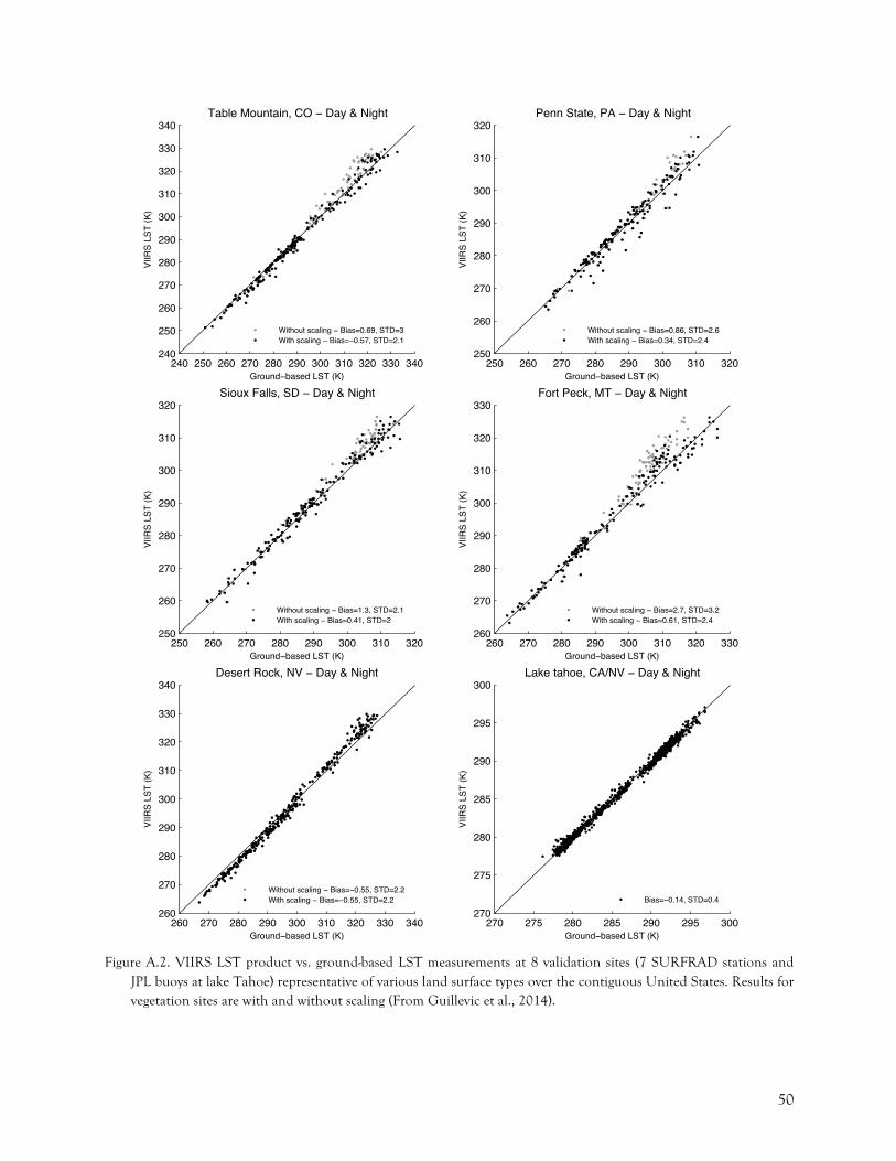
50
Figure A.2. VIIRS LST product vs. ground-based LST measurements at 8 validation sites (7 SURFRAD stations and
JPL buoys at lake Tahoe) representative of various land surface types over the contiguous United States. Results for vegetation sites are with and without scaling (From Guillevic et al., 2014).
240 250 260 270 280 290 300 310 320 330 340240
250
260
270
280
290
300
310
320
330
340
VIIR
S LS
T (K
)
Ground−based LST (K)
Table Mountain, CO − Day & Night
Without scaling − Bias=0.69, STD=3With scaling − Bias=−0.57, STD=2.1
250 260 270 280 290 300 310 320250
260
270
280
290
300
310
320
VIIR
S LS
T (K
)
Ground−based LST (K)
Penn State, PA − Day & Night
Without scaling − Bias=0.86, STD=2.6With scaling − Bias=0.34, STD=2.4
250 260 270 280 290 300 310 320250
260
270
280
290
300
310
320
VIIR
S LS
T (K
)
Ground−based LST (K)
Sioux Falls, SD − Day & Night
Without scaling − Bias=1.3, STD=2.1With scaling − Bias=0.41, STD=2
260 270 280 290 300 310 320 330260
270
280
290
300
310
320
330
VIIR
S LS
T (K
)
Ground−based LST (K)
Fort Peck, MT − Day & Night
Without scaling − Bias=2.7, STD=3.2With scaling − Bias=0.61, STD=2.4
260 270 280 290 300 310 320 330 340260
270
280
290
300
310
320
330
340
VIIR
S LS
T (K
)
Ground−based LST (K)
Desert Rock, NV − Day & Night
Without scaling − Bias=−0.55, STD=2.2With scaling − Bias=−0.55, STD=2.2
270 275 280 285 290 295 300270
275
280
285
290
295
300
VIIR
S LS
T (K
)
Ground−based LST (K)
Lake tahoe, CA/NV − Day & Night
Bias=−0.14, STD=0.4

51
7 REFERENCES Augustine, J. A., DeLuisi, J. J., and Long, C. N. (2000). SURFRAD—A national surface radiation budget
network for atmospheric research. Bulletin of the American Meteorological Society, 81, 2341–2357.
Augustine, J. A., Hodges, G. B., Cornwall, C. R., Michalsky, J. J., and Medina, C. I. (2005). An Up- date on SURFRAD—The GCOS Surface Radiation Budget Network for the Continental United States. Journal of Atmospheric and Oceanic Technology, 22, 1460–1472.
Allen, R. G., Tasumi, M., and Trezza, R. (2007). Satellite-based energy balance for mapping evapotranspiration with internalized calibration (METRIC)-model, Journal of Irrigation and Drainage Engineering, 133, 380-394.
Anderson, M.C., Norman, J.M., Diak, G.R., Kustas, W.P., & Mecikalski, J.R. (1997). A two-source time-integrated model for estimating surface fluxes using thermal infrared remote sensing. Remote Sens. Environment, 60, 195–216.
Anderson, M. C., C. R. Hain, B. D. Wardlow, A. Pimstein, J. R. Mecikalski and W. P. Kustas, (2011a). Evaluation of drought indices based on thermal remote sensing of evapotranspiration over the continental United States. Journal of Climate, 24, 2025-2044.
Anderson, M. C., Allen, R.G., Morse, A., & Kustas, W.P. (2012). Use of Landsat thermal imagery in monitoring evapotranspiration and managing water resources. Remote Sens. Environ., 122, 50-65.
Anderson, M.C., Kustas, W.P., Norman, J.M., Hain, C.R., Mecikalski, J.R., Schultz, L., Gonzalez-Dugo, M.P., Cammalleri, C., d'Urso, G., Pimstein, A., and Gao, F. (2011b). Mapping daily evapotranspiration at field to continental scales using geostationary and polar orbiting satellite imagery. Hydrology and Earth System Sciences, 15, 223-239.
Anderson, M.C., Hain, C.R., Jurecka, F., Trnka, M., Hlavinka, P., Dulaney, W., Otkin, J.A., Johnson, D., and Gao, F. (2016a). Relationships between the evaporative stress index and winter wheat and spring barley yield anomalies in the Czech Republic. Climate Research, 70, 215-230.
Anderson, M.C., Zolin, C.A., Sentelhas, P.C., Hain, C.R., Semmens, K., Yilmaz, M.T., Gao, F., Otkin, J.A., and Tetrault, R. (2016b). The Evaporative Stress Index as an indicator of agricultural drought in Brazil: An assessment based on crop yield impacts. Remote Sensing of Environment, 174, 82-99.
Baldridge, A.M., Hook, S.J., Grove, C.I., Rivera, G. (2009). The ASTER spectral library version 2.0. Remote Sensing of Environment 113, 711-715.
Barbosa, P.M., Pereira, J.M.C., and Gegoire, J.-M. (1998). Compositing Criteria for Burned Area Assessment Using Multitemporal Low Resolution Satellite Data. Remote Sensing of Environment, Vol. 65, pp. 38–49.
Barsi, J. A., Schott, J.R., Palluconi, F.D., Helder, D.L., Markham, B.L., Chander, G., and O'Donnell, E.M. (2003). Landsat TM and ETM+ Thermal Band Calibration, Canadian Journal of Remote Sensing, Vol. 29, No. 2 pp. 141-153.
Barsi, J.A., Hook, S.J., Schott, J.R., Raqueno, N.G., Markham, B.L. (2007). Landsat 5 Thematic Mapper Thermal Band Calibration Update, IEEE Geoscience and Remote Sensing Letters, Vol. 4, Number 4, pp. 552-555.
Barsi, J. A., Schott, J. R., Hook, S. J., Raqueno, N. G. Markham, B. L., and Radocinski, R. G. (2014). Landsat-8 Thermal Infrared Sensor (TIRS) vicarious Radiometric Calibration. Remote Sensing, 6, 11607-11626, doi:10.3390/rs61111607.
Basist, A., Grody, N.C., Peterson, T.C., and Williams, C.N. (1998). Using the Special Sensor Microwave/Imager to Monitor Land Surface Temperatures, Wetness, and Snow Cover. Journal of Applied Meteorology, Vol.37

52
Belward, A.S. (1996). The IGBP-DIS global 1 km land cover data set (DISCover)—Proposal and implementation plans. IGBP-DIS Office, Toulouse, France. IGBP-DIS working paper 13.
Cao, C., Weinreb, M. and Xu, H. (2004). Predicting simultaneous nadir overpasses among polar-orbiting meteorological satellites for the intersatellite calibration of radiometers. Journal of Atmospheric and Oceanic Technology, 21:4 537-542.
Caselles, V. and Sobrino, J.A. (1989). Determination of frosts in orange groves from NOAA-9 AVHRR data. Remote Sensing of Environment, vol. 29, no. 2, 135–146.
Cleugh, H.A., Leuning, R., Mu, Q., and Running, S.W. (2007). Regional evaporation estimates from flux tower and MODIS satellite data. Remote Sensing of Environment, Vol. 106, pp. 285–304.
Coll, C., Caselles, V., Galve, J. M., Valor, E., Niclo ̀s, R., Sanchez, J. M., et al. (2005). Ground measurements for the validation of land surface temperatures derived from AATSR and MODIS data. Remote Sensing of Environment, 97, 288–300.
Coll, C., Hook, S. J., and Galve, J. M. (2009a). Land surface temperature from the advanced Along-Track Scanning Radiometer: Validation over inland waters and vegetated surfaces. IEEE Transactions on Geoscience and Remote Sensing, 47, 350–360.
Coll, C., Wan, Z., and Galve, J. M. (2009b). Temperature-based and radiance-based validations of the V5 MODIS land surface temperature product. Journal of Geophysical Research, [Atmospheres], 114, D20102, http://dx.doi.org/10.1029/2009JD012038.
Coll, C., Galve, J. M., Sanchez, J. M., and Caselles, V. (2010). Validation of Landsat-7/ETM+ thermal-band calibration and atmospheric correction with ground-based measurements. IEEE Transactions on Geoscience and Remote Sensing, 48, 547–555.
Da Silva, J. R. M., Damasio, C. V., Sousa, A. M. O., Bugalho, L., Pessanha, L., Quaresma, P. (2015). Agriculture pest and disease risk maps considering MSG satellite data and land surface temperature, Int. J. App Earth Observation Geoinformation, 38, 40-50, doi: 10.1016/j.jag.2014.12.016
Dee, D.P., Uppala, S.M., Simmons, A.J., Berrisford, P., Poli, P., Kobayashi, S., Andrae, U., Balmaseda, M.A., Balsamo, G., Bauer, P., Bechtold, P., et al. (2011). The ERA-Interim reanalysis: configuration and performance of the data assimilation system. Quarterly Journal of the Royal Meteorological Society 137, 553-597.
Diamond, H. J., T. R. Karl, M. A. Palecki, C. B. Baker, J. E. Bell, R. D. Leeper, D. R. Easterling, J. H. Lawrimore, T. P. Meyers, M. R. Helfert, G. Goodge, and P. W. Thorne (2013). U.S. Climate Reference Network after one decade of operations: status and assessment. Bull. Amer. Meteor. Soc., 94, 489-498. doi: 10.1175/BAMS-D-12-00170.1
Dousset, B., and Gourmelon, F. (2003). Satellite multi-sensor data analysis of urban surface temperatures and landcover. Isprs Journal of Photogrammetry and Remote Sensing, 58, 43-54.
Dousset, B., Gourmelon, F., Laaidi, K., Zeghnoun, A., Giraudet, E., Bretin, P., Mauri, E., and Vandentorren, S. (2011). Satellite monitoring of summer heat waves in the Paris metropolitan area. International Journal of Climatology, 31, 313-323.
Ermida, S.L., Trigo, I.F., DaCamara, C.C., Go ̈ttsche, F.-M., Olesen, F.-S. and Hulley, G. (2014). Validation of remotely sensed surface temperature over an oak woodland landscape—The problem of viewing and illumination geometries. Remote Sensing of Environment, 148, 16-27.
Ermida, S.L., DaCamara, C. C., Trigo, I. F., Pires, A. C., Ghent, D., Remedios, J. (2017a). Modelling directional effects on remotely sensed land surface temperature. Remote Sens. Env., 190, 56-69. Doi: 10.1016/j.rse.2016.12.008

53
Ermida, S.L., Jimenez, C., Prigent, C., Trigo, I. F. and DaCamara, C. C. (2017). Inversion of AMSR-E observations for land surface temperature estimation - Part 2: Global comparison with infrared satellite temperature, J. Geophys. Res.,DOI: 10.1002/2016JD026148.
Fernandes, R., Plummer, S., Nightingale, J., Baret, F., Camacho, F., Fang, H., Garrigues, S., Gobron, N., Lang, M., Lacaze, R., LeBlanc, S., Meroni, M., Martinez, B., Nilson, T., Pinty, B., Pisek, J., Sonnentag, O., Verger, A., Welles, J., Weiss, M., & Widlowski, J.L. (2014). Global Leaf Area Index Product Validation Good Practices. Version 2.0. In G. Schaepman-Strub, M. Roma ́n, & J. Nickeson (Eds.), Best Practice for Satellite-Derived Land Product Validation (p. 76): Land Product Validation Subgroup (WGCV/CEOS), doi:10.5067/doc/ceoswgcv/lpv/lai.002
Fisher, J. B., K. P. Tu, and D. D. Baldocchi (2008). Global estimates of the land-atmosphere water flux based on monthly AVHRR and ISLSCP-II data, validated at 16 FLUXNET sites. Remote Sensing of Environment, 112(3), 901–919, doi:10.1016/j.rse.2007.06.025.
Freitas, S.C., Trigo, I.F., Bioucas-Dias, J.M., and Go ̈ttsche, F.-M. (2010). Quantifying the Uncertainty of Land Surface Temperature Retrievals From SEVIRI/Meteosat. IEEE Transactions on Geoscience and Remote Sensing, 48(1), 523-534.
Gallego-Elvira B., Olioso A., Mira M., Reyes- Castilloa, S., Boulet, G., et al., 2013. EVASPA (EVApotranspiration Assessment from SPAce) tool: An overview. Procedia Environmental Sciences, 19, 303–310.
Garcia-Haro, F. J., Sommer, S. and Kemper, T. (2005). Variable multiple endmember spectral mixture analysis (VMESMA). International Journal of Remote Sensing, vol. 26, no. 10, 2135–2162.
Garcia-Santos, V., Valor, E., Caselles, V., Mira, M., Galve, J.M. and Coll, C. (2013). Evaluation of Different Methods to Retrieve the Hemispherical Downwelling Irradiance in the Thermal Infrared Region for Field Measurements. IEEE Transactions on Geoscience and Remote Sensing, 51(4), 2155–2165.
GCOS-82, the Second Report on the Adequacy of the Global Observing Systems for Climate in Support of the UNFCCC, GCOS-82, April 2003 (WMO/TD No. 1143).
GCOS-200. The Global Observing System for Climate: Implementation Needs, 342PP. WMO, 2016. (available at https://library.wmo.int/opac/doc_num.php?explnum_id=3417)
Gillespie, A., Rokugawa, S., Matsunaga, T., Cothern, J. S., Hook, S. and Kahle, A. B. (1998). A temperature and emissivity separation algorithm for Advanced Spaceborne Thermal Emission and Reflection Radiometer (ASTER) images. IEEE Transactions on Geoscience and Remote Sensing, 36(4), 1113-1126, doi: 10.1109/36.700995.
Göttsche, F., Olesen, F. S., Hoyer, J. L., Wimmer, W., and Nightingale, T. (2017). Fiducial Reference Measurements for Validation of Surface Temperature from Satellites (FRM4STS) Technical Report TR-3: A framework to verify the field performance of TIR FRM. Reference OFE-D-120-V1-Iss-3-Ver-1-ISSUED, 75 pages.
Göttsche, F.-M., Olesen, F.-S., Trigo, I., Bork-Unkelbach, A., and Martin, M. (2016). Long Term Validation of Land Surface Temperature Retrieved from MSG/SEVIRI with Continuous in-Situ Measurements in Africa. Remote Sensing, 8, 410.
Goettsche, F. -M., Olesen, F. -S., and Bork-Unkelbach, A. (2013). Validation of land surface temperature derived from MSG/SEVIRI with in situ measurements at Gobabeb, Namibia. International Journal of Remote Sensing, 34(9–10), 3069–3083.
Goettsche, F. -M., and Hulley, G. C. (2012). Validation of six satellite-retrieved land surface emissivity products over two land cover types in a hyper-arid region. Remote Sensing of Environment, 124, 149–158.

54
Guillevic, P., Gastellu-Etchegorry, J. P., Demarty, J., and Prevot, L. (2003). Thermal infrared radiative transfer within three-dimensional vegetation covers. Journal of Geophysical Research, [Atmospheres], 108, 4248.
Guillevic, P. C., Privette, J. L., Coudert, B., Palecki, M.A., Demarty, J., Ottle ́, C., et al. (2012). Land Surface Temperature product validation using NOAA's surface climate observation networks - Scaling methodology for the Visible Infrared Imager Radiometer Suite (VIIRS). Remote Sensing of Environment, 124, 282–298, http://dx.doi.org/10. 1016/j.rse.2012.05.004.
Guillevic, P. C., Bork-Unkelbach, A., Go ̈ttsche, F. M., Hulley, G. C., Gastellu-Etchegorry, J. -P., Olesen, F. S., et al. (2013). Directional viewing effects on satellite Land Surface Temperature products over sparse vegetation canopies—A multisensor analysis. IEEE Geoscience and Remote Sensing Letters, 99, 1–5, http://dx.doi.org/10.1109/LGRS. 2013.2260319.
Guillevic, P. C., Biard, J., Hulley, G. C., Privette, J. L., Hook, S. J., Olioso, A., Göttsche, F.-M., Radocinski, R., Román, M. O., Yu, Y., and Csiszar I. (2014). Validation of Land Surface Temperature products derived from the Visible Infrared Imager Radiometer Suite (VIIRS) using ground-based and heritage satellite measurements. Remote Sensing of Environment, 154 (2014) 19–37, doi: 10.1016/j.rse.2014.08.013.
GUM-2008, Evaluation of measurement data — Guide to the expression of uncertainty in measurement, Joint Committee for Guides in Metrology (JCGM 100:2008, GUM 1995 with minor corrections), September 2008, http://www.bipm.org/utils/common/documents/jcgm/JCGM_100_2008_E.pdf.
Hain, C.R., Crow, W.T., Mecikalski, J.R., Anderson, M.C., and Holmes, T. (2011). An intercomparison of available soil moisture estimates from thermal infrared and passive microwave remote sensing and land surface modeling. Journal of Geophysical Research-Atmospheres, 116.
Hall, A., and Jones, G.V. (2010). Spatial analysis of climate in winegrape-growing regions in Australia. Australian Journal of Grape and Wine Research, 16, 389-404.
Hall, D.K., Comiso, J.C., DiGirolamo, N.E., Shuman, C.A., Key, J.R., and Koenig, L.S. (2012). A Satellite-Derived Climate-Quality Data Record of the Clear-Sky Surface Temperature of the Greenland Ice Sheet. Journal of Climate, 25, 4785-4798.
Hook, S. J., G. Chander, J. A. Barsi, R. E. Alley, A. Abtahi, F. D. Palluconi, B. L. Markham, R. C. Richards, S. G. Schladow, and D. L. Helder (2004). In-Flight Validation and Recovery of Water Surface Temperature with Landsat 5 Thermal Infrared Data Using an Automated High Altitude Lake Validation Site at Lake Tahoe CA/NV, USA. IEEE Transactions Geoscience and Remote Sensing, vol. 42, pp. 2767- 2776, 2004.
Hook, S. J., W. B. Clodius, L. Balick, R. E. Alley, A. Abtahi, R. C. Richards, and S. G. Schladow (2005). In-Flight Validation of Mid- and Thermal Infrared Data From the Multispectral Thermal Imager (MTI) Using an Automated High-Altitude Validation Site at Lake Tahoe CA/NV, USA. IEEE Transactions Geoscience and Remote Sensing, vol. 43, pp. 1991- 1999.
Hook, S. J., Vaughan, R. G., Tonooka, H., and Schladow, S. G. (2007). Absolute radiomet- ric in-flight validation of mid infrared and thermal infrared data from ASTER and MODIS on the Terra spacecraft using the Lake Tahoe, CA/NV, USA, automated validation site. IEEE Transactions on Geoscience and Remote Sensing, 45, 1798–1807.
Hulley, G. C., & Hook, S. J. (2009a). Intercomparison of versions 4, 4.1 and 5 of the MODIS Land Surface Temperature and emissivity products and validation with laboratory measurements of sand samples from the Namib Desert, Namibia. Remote Sensing of Environment, 133, 1313–1318.
Hulley, G. C., and Hook, S. J. (2009b). The North American ASTER Land Surface Emissivity Database (NAALSED) Version 2.0. Remote Sensing of Environment, 1967–1975.

55
Hulley, G. C., and Hook, S. J. (2010). Generating consistent Land Surface Temperature and emissivity products between ASTER and MODIS data for earth science research. IEEE Transactions on Geoscience and Remote Sensing, 1304–1315, http://dx.doi.org/ 10.1109/TGRS.2010.2063034.
Hulley, G. C., Hook, S. J., and Schneider, P. (2011). Optimized split-window coefficients for deriving surface temperatures from inland water bodies. Remote Sensing of Environment, 115, 3758–3769.
Hulley, G. C., Hughes, C. G., and Hook, S. J. (2012). Quantifying uncertainties in land surface temperature and emissivity retrievals from ASTER and MODIS thermal infrared data. Journal of Geophysical Research-Atmospheres, vol 117, pp. D23113- D23130.
Hulley, G., Veraverbeke, S., and Hook, S. (2014). Thermal-based techniques for land cover change detection using a new dynamic MODIS multispectral emissivity product (MOD21). Remote Sensing of Environment, 140, 755-765.
Islam I., Hulley, G. C., Malakar, N. K., Radocinski, R. G., Hook, S. J. and Guillevic, P. C. (2017). A physics-based algorithm for the simultaneous retrieval of land surface temperature and emissivity from VIIRS thermal infrared data, IEEE Transactions on Geoscience and Remote Sensing, 55, 1, 563-576.
Jacob, F., Petitcolin, F., Schmugge, T., Vermote, E., French, A., and Ogawa, K. (2004). Comparison of land surface emissivity and radiometric temperature derived from MODIS and ASTER sensors. Remote Sensing of Environment, 90, 137–152.
Jedlovec, G.J. Haines, S.L., and LaFontaine, F.J. (2008). Spatial and Temporal Varying Thresholds for Cloud Detection in GOES Imagery. IEEE Transactions on Geoscience and Remote Sensing, V. 46, N. 6.
Jimenez, C., Prigent, C., Ermida, S. L. and Moncet, J.-L. (2017) Inversion of AMSR-E observations for land surface temperature estimation - Part 1: Methodology and evaluation with station temperature, J. Geophys. Res. DOI: 10.1002/2016JD026144.
Jiménez-Muñoz, J.C., and Sobrino, J.A. (2007). Emissivity spectra obtained from field and laboratory measurements using the temperature and emissivity separation algorithm. Applied Optics, 45, 7104–7109.
Jones, G.V., Duff, A.A., Hall, A., and Myers, J.W. (2010). Spatial Analysis of Climate in Winegrape Growing Regions in the Western United States. American Journal of Enology and Viticulture, 61, 313-326.
Kalma, J.D., McVicar, T.R., and McCabe, M.F. (2008). Estimating Land Surface Evaporation: A Review of Methods Using Remotely Sensed Surface Temperature Data. Surv Geophys, Vol.29, pp.421–469.
Kalnay, E., Kanamitsu, M., Kistler, R., Collins, W., 1996. The NCEP/NCAR 40-year reanalysis project. Bulletin of the American Meteorological Society 77, 437-471.
Kealy, P.S., and Hook, S. (1993). Separating temperature & emissivity in thermal infrared multispectral scanner data: Implication for recovering land surface temperatures. IEEE Transactions on Geoscience and Remote Sensing, 31, 1155-1164.
Kogan, F.N. (1995). Application of vegetation index and brightness temperature for drought detection. Advances in Space Research, 15(11), 91–100.
Kogan, F.N. (1997). Global drought watch from space. Bulletin of the American Meteorological Society, 78(4), 621–636.
Kondratyev, K. Y., (1969). Radiation in the Atmosphere. International geophysics series, vol. 12, New York, NY; London: Academic Press.
Korb, A. R., Salisbury, J. W., and D'Aria, D. M. (1999). Thermal-infrared remote sensing and Kirchhoff's law 2. Field measurements. Journal of Geophysical Research-Solid Earth, 104(B7), 15339−15350.
56
Krehbiel, C., and Henebry, G.M. (2016). A Comparison of Multiple Datasets for Monitoring Thermal Time in Urban Areas over the US Upper Midwest. Remote Sensing, 8.
Lambin, E.F., and Ehrlich, D. (1997). Land-cover Changes in Sub-Saharan Africa (1982-1991): Application of a Change Index Based on Remotely Sensed Surface Temperature and Vegetation Indices at a Continental Scale. Remote Sensing of Environment, Vol.61, pp. 181–200.
Li, Z. -L., Tang, B. H., Wu, H., Ren, H. Z., Yan, G. J., Wan, Z. M., et al. (2013). Satellite-derived land surface temperature: Current status and perspectives. Remote Sensing of Environment, 131, 14–37, http://dx.doi.org/10.1016/j.rse.2012.12.008.
Li, H., Sun, D., Yu, Y., Wang, H., Liu, Y., Liu, Q., et al. (2014). Evaluation of the VIIRS and MODIS LST products in an arid area of Northwest China. Remote Sensing of Environment, 142, 111–121, http://dx.doi.org/10.1016/j.rse.2013.11.014.
Llewellyn-Jones, D., Edwards, M., Mutlow, C., Birks, A., Barton, I., Tait, H., 2001. AATSR: global-change and surface-temperature measurements from ENVISAT. ESA bulletin 105, 10–21.
Luvall, J., Quattrochi, D.A., Rickman, D., and Estes, M.G. (Eds.) (2015). Urban Heat Islands: Encyclopedia of Atmospheric Sciences.
Malakar, N., and Hulley, G. (2016). A Case Study of Warming Trends and Spatial Patterns of Land Surface Temperatures over the Greater Los Angeles Area Using a new MODIS LST product In, American Geophysical Union (AGU). San Francisco, CA.
Martin, M. A., and Göttsche, F.-M. (2016). Satellite LST Validation Report (DEL-13). ESA DUE GlobTemperature Project, reference GlobT-WP4-DEL-12, www.globtemperature.info.
Martin, M. A., Göttsche, F.-M., Ghent, D., Trent, T., Dodd, E., Pires, A., Trigo, I., Prigent, C. and Jimenez, C. (2016). Satellite LST Intercomparison Report (DEL-13). ESA DUE GlobTemperature Project, reference GlobT-WP4-DEL-13, www.globtemperature.info.
Matricardi, M. (2009). Technical Note: An assessment of the accuracy of the RTTOV fast radiative transfer model using IASI data. Atmospheric Chemistry and Physics, 9, 6899-6913.
Matsunaga, T. (1994). A temperature-emissivity separation method using an empirical relationship between the mean, the maximum, & the minimum of the thermal infrared emissivity spectrum, in Japanese with English abstract. Journal Remote Sensing Society Japan, 14, 230-241.
Merchant, C. J., Matthiesen, S., Rayner, N. A., Remedios, J. J., Jones, P. D., Olesen, F., et al. (2013). The surface temperatures of Earth: Steps towards integrated understanding of variability and change. Geoscientific Instrumentation Methods and Data Systems, 2(305–321), 2013, http://dx.doi.org/10.5194/gi-2-305-2013.
Mildrexler, D.J., Zhao, M., Heinsch, F.A., and Running, S.W. (2007). A new satellite-based methodology for continental-scale disturbance detection. Ecological Applications, V.17, pp. 235–250.
Mu, Q., Zhao, M., Kimball, J. S., McDowell, N. G., and Running, S. W. (2013). A Remotely Sensed Global Terrestrial Drought Severity Index. Bulletin of the American Meteorological Society, 01/2013, Vol. 94, Issue 1, Number 1, 83-98, DOI:10.1175/BAMS-D-11-00213.1.
Neteler, M. (2005). Time Series Processing of MODIS Satellite Data for Landscape Epidemiological Applications. International Journal of Geoinformatics, Vol.1, No.1, ISSN 1686–6576.
Neteler, M., Roiz, D., Rocchini, D., Castellani, C., and Rizzoli, A. (2011). Terra and Aqua satellites track tiger mosquito invasion: modelling the potential distribution of Aedes albopictus in north-eastern Italy. International Journal of Health Geographics, 10.
Niclòs, R., Galve, J.M., Valiente, J.A., Estrela, M.J., Coll, C., 2011. Accuracy assessment of land surface temperature retrievals from MSG2-SEVIRI data. Remote Sensing of Environment 115, 2126-2140.

57
Nishida, K., Nemani, R.R., Running, S.W., and Glassy, J.M. (2003). An operational remote sensing algorithm of land surface evaporation. Journal of Geophysical Research, Vol.108, No. D9, 4270
Norman, G., and Becker, F. (1995). Terminology in thermal infrared remote sensing of natural surfaces. Agricultural and Forest Meteorology, Volume: 77, Issue: 3-4, Pages: 153-166, DOI: 10.1016/0168-1923(95)02259-Z.
Ouyang, X., Chen, D., Duan, S.-B., Lei, Y., Dou, Y., and Hu, G. (2017). Validation and Analysis of Long-Term AATSR Land Surface Temperature Product in the Heihe River Basin, China. Remote Sensing, 9(152), 1-18, doi:10.3390/rs9020152.
Orth, R., Dutra, E., Trigo, I. F. and Balsamo, G. (2017). Advancing land surface model development with satellite-based Earth observations, Hydrol. Earth Syst. Sci., 21, 2483–2495, Doi: 10.5194/hess-21-2483-2017.
Pasotti, L., Maroli, M., Giannetto, S., and Brianti, E. (2006). Agrometeorology and models for the parasite cycle forecast. Parassitologia, 48, 81-83.
Pinheiro, A.C.T., Privette, J. L., and Guillevic, P. (2006). Modeling the observed angular anisotropy of land surface temperature in a savanna. IEEE Transactions on Geoscience and Remote Sensing, 44(4), 1036–1047 (April 2006).
Peres, L.F. and DaCamara, C.C. (2005). Emissivity maps to retrieve land-surface temperature from MSG/SEVIRI. IEEE Transactions on Geoscience and Remote Sensing, vol. 43, no. 8, 1834–1844.
Peres, L.F., Libonati, R., and DaCamara, C.C. (2014). Land-Surface Emissivity Retrieval in MSG–SEVIRI TIR Channels Using MODIS Data. IEEE Transactions on Geoscience and Remote Sensing, vol. 52, no.9, 5587–5600.
Prata, A. J. (1994). Land surface temperatures derived from the advanced very high resolution radiometer and the along-track scanning radiometer: 2. Experimental results and validation of AVHRR algorithms. Journal of Geophysical Research: Atmospheres, 99(D6), 13025–13058.
Prata, F., 2002. Land surface temperature measurement from space: AATSR algorithm theoretical basis document. CSIRO Atmospheric Research, Aspendale, Australia.
Randolph, S., Green, R., Peacey, M. and Rogers, D., (2000). Seasonal synchrony: The key to tick-borne encephalitis foci identified by satellite data. Parasitology, Vol. 121, pp. 15–23.
Rasmussen, M.O., Gottsche, F.M., Olesen, F.S., and Sandholt, I. (2011). Directional effects on land surface temperature estimation from Meteosat Second Generation for savanna landscapes IEEE Transactions on Geoscience and Remote Sensing 49 (11), 4458-4468.
Remedios, J. (2012). SLSTR ATBD Land Surface Temperature, Sentinel-3 Optical Products and Algorithm Definition, Version 2.3, ref. S3-L2-SD-03-T03-ULNILU-ATBD_L2LST, Oct. 10, 2012, https://sentinel.esa.int/documents/247904/349589/SLSTR_Level-2_LST_ATBD.pdf.
Rienecker, M. R., Suarez, M. J., Gelaro, R., Todling, R., Bacmeister, J., Liu, E., Bosilovich, M. G., Schubert, S. D. et al., (2011) MERRA: NASA's Modern-Era Retrospective Analysis for Research and Applications. Journal of Climate, 24, 3624–3648, doi:10.1175/JCLI-D-11-00015.1.
Rojas, O., Vrieling, A., and Rembold, F. (2011). Assessing drought probability for agricultural areas in Africa with coarse resolution remote sensing imagery. Remote Sensing of Environment, 115, 343–352.
Roy, D.P. (1997). Investigation of the maximum Normalized Difference Vegetation Index (NDVI ) and the maximum surface temperature (Ts ) AVHRR compositing procedures for the extraction of NDVI and Ts over forest. International Journal of Remote Sensing, Vol.18, No.11, pp.2383–2401.
Rubio, E., Caselles, V., Coll, C., Valour, E., and Sospedra, F. (2003). Thermal-infrared emissivities of natural surfaces: Improvements on the experimental set-up and new measurements. International Journal of Remote Sensing, 24(24):5379–5390.

58
Sabol, D.E., Gillespie, A.R., Abbott, E., & Yamada, G. (2009). Field validation of the ASTER Temperature-Emissivity Separation algorithm. Remote Sensing of Environment, 113, 2328-2344.
Sandholt, I., Rasmussen, K., and Andersen, J. (2002). A simple interpretation of the surface temperature / vegetation index space for assessment of surface moisture status. Remote Sensing of Environment, Vol. 79, pp. 213–224.
Schneider, P., Ghent, D., Corlett, G., Prata, F., and remedies, J. (2012). AATSR validation: LST validation protocol. Internal publication, UL-NILU-ESA-LST-LVP Issue 1 Revision 0, page 1-39. http://lst.nilu.no/Portals/73/Docs/Reports/UL-NILU-ESA-LST-LVP-Issue1-Rev0-1604212.pdf.
Schneider, P., and Hook, S.J. (2010). Space observations of inland water bodies show rapid surface warming since 1985. Geophysical Research Letters, 37.
Semmens, K.A., Anderson, M.C., Kustas, W.P., Gao, F., Alfieri, J.G., McKee, L., Prueger, J.H., Hain, C.R., Cammalleri, C., Yang, Y., Xia, T., Sanchez, L., Alsina, M.M., and Velez, M. (2016). Monitoring daily evapotranspiration over two California vineyards using Landsat 8 in a multi-sensor data fusion approach. Remote Sensing of Environment, 185, 155-170.
Schott, J. R., Hook, S. J., Barsi, J. A., Markham, B. L., Miller, J., Padula, F.P., and Raqueno, N.G. (2012). Thermal infrared radiometric calibration of the entire Landsat 4, 5, and 7 archive (1982–2010). Remote Sensing of Environment, 122, 41–49.
Schmugge, T., and Ogawa, K. (2006). Validation of emissivity estimates from ASTER and MODIS data. Proceedings of 2006 International Geoscience and Remote Sensing Symposium (pp. 260−262).
Singh, R.P., Roy, S., and Kogan, F. (2003). Vegetation and temperature condition indices from NOAA AVHRR data for drought monitoring over India. International Journal of Remote Sensing, 20(22), 4393–4402.
Sobrino, J. S. and Caselles, V., (1993). A field method for measuring the thermal infrared emissivity. ISPRS Journal of Photogrammetry and Remote Sensing 48, 24–31.
Sobrino, J.A. and Cuenca, J. (1999). Angular Variation of Thermal Infrared Emissivity for Some Natural Surfaces from Experimental Measurements. Applied Optics, 1999. 38, 3931– 36.
Sobrino, J.A. and El Kharraz, MH. (1999). Combining afternoon and morning NOAA satellites for thermal inertia estimation: 1. Algorithms and its testing with Hydrologic Atmospheric Pilot Experiment-Sahel data. Journal of Geophysical Research, 104. D8, 9445– 9453.
Sobrino, J.A., Jime ́nez-Munoz, J. C., and Verhoef, W. (2005). Canopy directional emissivity: Comparison between models. Remote Sensing of Environment, 99, 304–314.
Sobrino, J.A., Jime ́nez-Mun ̃oz, J. C., Balick, L., Gillespie, A.R., Sabol, D. A., and Gustafson, W. T. (2007). Accuracy of ASTER level-2 thermal-infrared standard products of an agricultural area in Spain. Remote Sensing of Environment, 106, 146–153.
Sobrino, J. A., Oltra-Carrió, R., Soria G., Jiménez-Muñoz, J. C., Franch, N., Hidalgo, V. et al. (2013). Evaluation of the surface urban heat island effect in the city of Madrid by thermal remote sensing. International Journal of Remote Sensing, 34, 3177-3192.
Sobrino, J. A., and Skokovic, D. (2016). Permanent Stations for Calibration/Validation of Thermal Sensors over Spain, Data, 1, 10; doi:10.3390/data1020010.
Sobrino, J. A., Del Frate, F., Drusch, M., Jiménez-Muñoz, J. C., Manunta, P., Regan, A. (2016). Review of Thermal infrared applications and requirements for future high-resolution sensors, IEEE Transactions on Geoscience and Remote Sensing, 54, 2963-2972.
Snyder, W. C., Wan, Z., Zhang, Y., and Feng, Y. -Z. (1998). Classification-based emissivity for land surface temperature measurement from space. International Journal of Remote Sensing, 19(14), 2753–2774.

59
Stöckli, R. (2013). The HelioMont Surface Solar Radiation Processing, Scientific Report MeteoSwiss, 93, ISSN: 1422–138, 122 pp.
Suarez, M., and Bacmeister, J., 2015: Development of the GEOS-5 atmospheric general circulation model: evolution from MERRA to MERRA2, Geoscientific Model Development, 8, 1339-1356.
Theocharous, E., Fox, N. Göttsche, F., Hoyer, J. L., Wimmer, W., and Nightingale, T. (2016). Fiducial Reference Measurements for Validation of Surface Temperature from Satellites (FRM4STS) Technical Report TR-1: Procedures and Protocols for the verification of TIR FRM Field Radiometers and Reference Blackbody Calibrators. Reference: OFE- D80-V1-Iss-3-Ver-1-FINAL, 104 pages.
Tonooka, H. (2005). Accurate atmospheric correction of ASTER thermal infrared imagery using the WVS method, IEEE Transactions on Geoscience and Remote Sensing, vol. 43, pp. 2778-2792.
Trigo, I.F., Boussetta, S., Viterbo, P., Balsamo, G., Beljaars, A., Sandu, I. (2015). Comparison of model land skin temperature with remotely sensed estimates and assessment of surface-atmosphere coupling, J. Geophys. Res., 120, doi: 10.1002/2015JD023812.
Trigo, I. F., Monteiro, I. T., Olesen, F., and Kabsch, E. (2008). An assessment of remotely sensed land surface temperature. Journal of Geophysical Research, [Atmospheres], 113, http://dx.doi.org/10.1029/2008JD010035 D17108.
Unsworth, M.H. (1975). Long-wave radiation at the ground. II. Geometry of interception by slopes, solids and obstructed planes. Quarterly Journal of the Royal Meteorological Society, 101, 25–34.
Uppala, S.M., Kållberg, P.W., Simmons, A.J., Andrae, U., Da Costa Bechtold, V., Fiorino, M., Gibson, J.K., Haseler, et al. (2005). The ERA-40 re-analysis. Quarterly Journal of the Royal Meteorological Society 131, 2961-3012.
Wan, Z. (2008). New refinements and validation of the MODIS land-surface temperature/ emissivity products. Remote Sensing of Environment, 112, 59–74.
Wan, Z., and Dozier, J. (1996). A generalized split-window algorithm for retrieving land surface temperature from space. IEEE Transactions on Geoscience and Remote Sensing, 34, 892–905.
Wan, Z., and Li, Z. -L. (2008). Radiance-based validation of the V5 MODIS land-surface temperature product. International Journal of Remote Sensing, 29, 5373–5393.
Wan, Z. (2014). New refinements and validation of the collection-6 MODIS land-surface temperature/emissivity product. Remote Sensing of Environment, 140, 36–45, http:// dx.doi.org/10.1016/j.rse.2013.08.027.
Wang, W., Liang, S., and Meyers, T. P. (2008). Validating MODIS land surface temperature products using long-term nighttime ground measurements. Remote Sensing of Environment, 112, 623–635.
Wang, K., and Liang, S. (2009). Evaluation of ASTER and MODIS land surface temperature and emissivity products using long-term surface longwave radiation observations at SURFRAD sites. Remote Sensing of Environment, 113(7), 1556–1565.
Wang, Z., Schaaf, C. B., Strahler, A. H., Chopping, M. J., Roma ́n, M.O., Shuai, Y., et al. (2014). Evaluation of MODIS albedo product (MCD43A) over grassland, agriculture and forest surface types during dormant and snow-covered periods. Remote Sensing of Environment, 140, 60–77.
Wolfe, R.E., Lin, G., Nishihama, M., Tewari, K.P., Tilton, J.C., and Isaacman, A.R. (2013). Suomi NPP VIIRS prelaunch and on-orbit geometric calibration and characterization. Journal of Geophysical Research: Atmospheres, 2013JD020508, 10.1002/jgrd.50873.
Xu, H., Yu, Y., Tarpley, D., Göttsche, F.-M and Olesen, F.-S. (2014), Evaluation of GOES-R Land Surface Temperature Algorithm Using SEVIRI Satellite Retrievals With In Situ Measurements. IEEE Transactions on Geoscience and Remote Sensing, Vol. 52, No. 7,Doi: 10.1109/TGRS.2013.2276426.

60
Yu, Y., Privette, J. L., and Pinheiro, A. (2005). Analysis of the NPOESS VIIRS Land Surface Temperature algorithm using MODIS data. IEEE Transactions on Geoscience and Remote Sensing, Vol. 43, No. 10, 2340-2350.
Zheng, W., Wei, H., Wang, Z., Zeng, X., Meng, J., Ek, M., Mitchell, K. and Derber, J. (2012). Improvement of daytime land surface skin temperature over arid regions in the NCEP GFS model and its impact on satellite data assimilation. J. Geophys. Res, 117, D06117, Doi: 10.1029/2011JD015901.
Zhou, L., Dickinson, R.E., Tian, Y., Jin, M., Ogawa, K., Yu, H., and Schmugge, T. (2003). A sensitivity study of climate and energy balance simulations with use of satellite-derived emissivity data over Northern Africa and the Arabian Peninsula. Journal of Geophysical Research-Atmospheres, 108, 4795.
Zorer, R., Rocchini, D., Metz, M., Delucchi, L., Zottele, F., Meggio, F., and Neteler, M. (2013). Daily MODIS Land Surface Temperature Data for the Analysis of the Heat Requirements of Grapevine Varieties. Ieee Transactions on Geoscience and Remote Sensing, 51, 2128-2135.