LAND COVER DEPENDENT DERIVATION OF DIGITAL …

LAND COVER DEPENDENT DERIVATION OF DIGITAL SURFACE MODELS FROM AIRBORNE LASER SCANNING DATA

Hollaus M.a,*,

Mandlburger G.a, Pfeifer N.a, Mücke W.a

a TU Wien - Vienna University of Technology, Institute of Photogrammetry and Remote Sensing (I.P.F.)

Gusshausstraße 27-29, 1040 Vienna, Austria (mh, gm, np, wm)@ipf.tuwien.ac.at

Commission III, WG III/2

KEY WORDS: DEM/DTM, nDSM, LiDAR, Forestry, Vegetation, Surface, Model, Building ABSTRACT In contrast to the algorithms for determining digital terrain models (DTMs) from airborne laser scanning (ALS) data, those for the generation of digital surface models (DSMs) are rather straightforward. A common way to derive DSMs is the determination of the highest point within a defined raster cell (DSMmax) or the determination of the DSM heights based on moving least squares interpolation e.g. moving planes (DSMmls). For low ALS point densities void pixels can occur in the DSMmax and for inclined smooth surfaces the DSMmax shows an artificial roughness mainly due to the irregular point distribution. These disadvantages of the DSMmax can be reduced by using an interpolated grid DSMmls. On the other hand, the DSMmls introduces smoothing effects along surface discontinuities e.g. building borders, tree tops, forest gaps, etc. In this paper a combined approach for the DSM generation is presented, which makes use of the strengths of both, the DSMmax and the DSMmls. The used algorithms are implemented in the scientific software package OPALS (Orientation and Processing of Airborne Laser Scanning data). The proposed processing chain for DSM determination is applied for four test sites in Austria with different land cover types. For these test sites ALS data with point densities between 5.5 and 60.0 echoes per m2 are available. The derived DSMs are presented and compared to traditional DSMs. Especially, for deciduous forests the difference between the single DSMs can add up to several metres.

* Corresponding author.

1. INTRODUCTION

Different topographic models derived from 3D point clouds, acquired either by airborne laser scanning (ALS) or by stereo matching of aerial images, are in use today. The most commonly used model is the digital terrain model (DTM) describing the elevation of the ground surface. In contrast to the DTM, the digital surface model (DSM) represents the topmost surface which can be seen from the acquisition platform (e.g. aeroplane, helicopter). The DSM and the DTM are equivalent in open areas like streets, agricultural fields without vegetation, grassland with “short” vegetation, or areas with bare soil. For areas, which are covered with buildings the DSM describes the roofs whereas the DTM describes the terrain without buildings. In forested areas the DTM represents the ground surface and the DSM the elevation of the top most canopy surface. A subsequent product is the normalised digital surface model (nDSM) calculated by subtracting the DTM from the DSM. Therefore, the nDSM contains object heights such as building and tree heights and is used in several applications e.g. building detection, building height estimation, forest delineation, tree height estimation, stem volume and above ground biomass assessment. For forestry applications the term digital canopy model (DCM) and the normalized canopy model (nCM) are equivalently in use instead of DSM and nDSM respectively.

For the calculation of a DTM the measured 3D points have to be classified into terrain and off-terrain echoes, a process that is commonly referred to as filtering (Pfeifer et al., 1998). In the past several filtering techniques (Sithole and Vosselman, 2004) were developed, which are commonly based on the spatial relationship of the 3D echoes. In contrast to the algorithms for determining DTMs, the algorithms for DSM generation are rather simple. The first echo points are typically used without further discrimination. Common ways for deriving DSMs with a grid structure include choosing the highest elevation within a defined raster cell or the arithmetic mean of the heights. Alternatively, the determination of grid heights can exploit a surface function, for example the triangulation of the points with linear interpolation within each triangle, as e.g. implemented in the “natural neighbour” package NN (Fan et al, 2005). Finally, the general approach of moving least squares (Lancaster and Šalkauskas, 1990), is applied in DSM computation, e.g., the moving least squares interpolation as implemented within the OPALS (2010) fits a tilted plane to the eight nearest neighbouring first-echo points by using least squares. Furthermore, the heights are weighted inversely proportional to the distance from the grid point.

In: Paparoditis N., Pierrot-Deseilligny M., Mallet C., Tournaire O. (Eds), IAPRS, Vol. XXXVIII, Part 3A – Saint-Mandé, France, September 1-3, 2010Contents Keyword index Author index

221

In order to obtain the DTM from classified ground points the interpolation techniques applied often consider the properties of the terrain, e.g. in the variogram of kriging or in the neighbourhood size of local interpolation methods. For high demands break lines and peak heights may be inserted at those locations where the global assumptions on the terrain are violated, e.g. the assumptions on smoothness. For surface models the situation is more complex as different objects, including terrain, roofs, vegetation canopy, etc., have to be considered. The surfaces of these objects have different properties, which have effect on the appropriate interpolation method. Examples include the treatment of height jumps, methods for filling data gaps, or what constitutes an outlier. Additionally, the sampling interval may become relatively low for some objects, e.g. individual trees, which suggests that no or only minimal filtering of random measurement errors shall be performed. Thus, applying one of the DSM computation methods listed above with only one set of parameters, can hardly fulfil the different interpolation demands arising from different object surfaces. The following two approaches for calculating DSMs shall demonstrate this.

• For areas with surfaces discontinuities e.g. along breaklines, step edges or forests the DSM calculation based on the highest point within a defined raster cell (DSMmax) leads to a good approximation of the real surface. As shown in Fig. 1a the DSMmax values are near to the tree tops and near to the terrain within forest gaps. Furthermore, the DSMmax represents the surface in a proper form along building edges and roof ridges (Fig. 1b). On the other hand, for inclined smooth surfaces (Fig. 1b) the derived DSMmax leads to an artificial surface roughness and to an overestimation of the modelled surface.

• In contrast to the DSMmax, the surface height calculation based on moving least squares interpolation (DSMmls) smoothes surface discontinuities as illustrated in Fig. 1a (1-3). On the other hand the DSMmls represents a good approximation of inclined smooth surfaces (Fig. 1b).

Obviously, a mixture of both models would be the best choice in the above examples, with the DSMmls used for smooth surfaces (e.g. street and roof) and the DSMmax for rough surfaces (e.g. the high vegetation areas). However, due to the missing semantic information of the acquired data, the land cover (class) of the recorded echoes is unknown in advance. The contribution of this article is a conceptual framework, its methods, and the description of a specific implementation for the computation of improved DSMs. Based on (i) land cover proxies and (ii) properties of the data coverage (e.g. gaps), different algorithms for the DSM computation are applied. The algorithms used are not new, but it is pointed out that the synthesis of methods is the key idea presented in this paper. The overall aim is to generate DSMs, which allow improving visual analysis and algorithms working on the DSM and nDSM. In section 2 the conceptual framework and its specialization addressing the above examples are presented. This section also includes the implementation within OPALS (2010).

Figure 1. Illustration of DSM calculations based on the highest point within a defined raster cell (DSMmax) and moving least

squares interpolation (DSMmls) for a forested area (a) and for a building roof (b). In (a) the DSMmls underestimates the heights

of tree tops and overestimates the heights of the terrain for forest gaps. In (b) the DSMmax overestimates the inclined roof

plane and introduce an artificial roughness.

Depending on the surface roughness either the DSMmax or the DSMmls is used for the determination of the DSM height. The supposed work flow is applied for different ALS data (e.g. discrete, full-waveform) with different point densities for Austrian test sites located in forests, agricultural land and urban areas as introduced in section 3. In section 4 the examples are presented and compared to traditional DSMs.

2. METHODS

The basic principle of the suggested approach is to first apply data analysis on the original point cloud and – depending on its outcome – chose different algorithms for DSM computation (see also Fig. 2). Each analysis step results in a layer (l1, ...) with qualitative or quantitative information, all together nl layers. A rule-based analysis of the different layers at each grid position selects the appropriate interpolation method (m1, ...), from all together nm methods. This can also be seen as selecting the elevation of a specific (primary) surface model computed for the entire area. In contrast to the layer data, the surface model values must be metric. The rules for selecting the appropriate elevation are provided by an expert. Such a rule may be to choose a specific method/model, but also the combination of different methods (e.g. the average) might be feasible.


222

Figure 2. Concept of DSM generation considering different data

properties (layers l1 to lnl) and different models (m1 to mnm).

The general case is, thus, to define the final surface model as a function f of the layers and the primary surface models. For evaluating the function at a specific (x,y) location, the arguments are the values of the layers l1(x,y), ... lnl(x,y), and the values of the models m1(x,y), ... mnm(x,y). The return value of f has to be metric, too. More specifically, to be interpretable as a surface model, f (x,y) has to be within the minimum-maximum range of m1(x,y), ... mnm(x,y). The layers and the surface models may be derived as cell information (raster data) or as grids (vector data). For the computation of DSMs, several interpolation algorithms are available. Amongst the interpolation methods considered useful for topographic point clouds are Moving Least Squares, Inverse Distance Weighting, Kriging, gridding of a triangulation, etc. In the specific approach presented in this paper, the function f shall be used to choose the DSM computed with an interpolation method suitable for the specific land cover class found at the grid post. The surface roughness was chosen, because it discriminates between street, house roofs, and open areas on the one hand, and strongly vegetated and rocky surfaces on the other hand. Thus only 2 groups, each representing a number of land cover classes, are formed, and therefore, two DSMs are computed. 2.1 Implementation within OPALS

OPALS (Orientation and Processing of Airborne Laser Scanning data) is a scientific software project developed at the Institute of Photogrammetry and Remote Sensing (I.P.F), TU Vienna (Mandlburger et al., 2009). The aim of OPALS is to provide a complete workflow for processing large ALS projects. OPALS targets the following topics: processing of raw sensor data, quality control, georeferencing, modelling of structure lines, filtering of ALS point clouds, DTM interpolation, and subsequent applications like city modelling, forestry, hydraulics etc. OPALS is a modular system consisting of small units (modules), each covering a well defined task. A software frame work is responsible for providing each module in three different implementations: (i) as command-line executable, (ii) as Python module (Phyton, 2010), and (iii) as C++-class library via DLL

linkage. Arbitrary workflows can be constructed by embedding the respective OPALS modules in a scripting environment. To handle ALS data in the order of >109 points, a central data management component (OPALS Data Manager, ODM) was developed, providing efficient spatial data access and an administration concept for storing arbitrary point attributes (e.g. echo width, amplitude, classification, normal vector, etc.). In this study, the modules opalsCell, opalsGrid and opalsAlgebra are used to derive a land cover dependent DSM. 2.2 Land cover dependent calculation of DSMs

The module opalsCell is a raster based analysis tool accumulating specific features (min, max, mean, etc.) of a selected point attribute (z, amplitude, echo width, etc.). For the work at hand, first a DSM raster containing the maximum elevation of all points within a cell (DSMmax) was derived. The aim of opalsGrid is to derive digital surface or terrain models (DSM/DTM) in regular grid structure using simple interpolation techniques like moving least squares, nearest neighbour or moving average. In our study we used the moving least squares interpolation with a plane as functional model, i.e., a tilted regression plane is fitted through the k-nearest neighbours (k). Apart from the elevation (DSMmls), the moving least squares interpolation allows for the derivation of additional features per grid post. Among these features are the standard error of the estimated grid post elevation (σz, roughness indicator) and the eccentricity (distance: grid point – centre of gravity of input points). These attributes have proven their worth in subsequent processing steps, especially to detect occluded and vegetated areas. 2.3 Land cover dependent combination of DSMs

For the land cover dependent combination of the DSMs the module opalsAlgebra is employed to derive a grid or raster model by combining multiple input grid and/or raster data sets. The cell values are calculated by applying an algebraic formula based on the values of the respective input grids. Any mathematical formula, and even an entire program code returning a scalar value, can be passed. In this study, we assume that the σz-layer can be used to classify the area in rough and smooth surfaces. Therefore, we combine the DSMmax and the DSMmls depending on the corresponding σz-layer. The heights (z) of the land cover dependent DSM are calculated by (pseudo code):

z[DSM] = z[σz] < 0.2 or not z[DSMmax] ? z[DSMmls] : z[DSMmax]

3. STUDY AREA AND DATA

The proposed work flow is applied to four test sites located in Vienna (parts of the Schönbrunn Palace), lower Austria (north of the Ötscher mountain), Burgenland (Neusiedler See) and Vorarlberg (Montafon region), Austria. For the first three test sites full-waveform ALS data sets are available. For the first two test sites the ALS data is acquired with a Riegl LMS-Q560. For the Burgenland test site a Riegl LMS-Q680 was used (Riegl, 2010). The ALS data acquisition took place under leaf-off conditions. The point density (echoes per m2) is approx. 60 and approx. 20 for the Vienna and lower Austria / Burgenland test site respectively. For the Vorarlberg test site, ALS data with a point density of approx. 5.5 echoes per m2 are available and the discrete echoes were acquired as first and last echoes. This


223

data set was acquired with an Optech ALTM 1225 and an ALTM 2050 (Optech, 2010). The Vienna test site covers parts of the Schönbrunn garden area as well as build-up areas. The investigated area in lower Austria is characterized by a varying landscape featuring steep slopes, deep valleys and basins. The densely forested area is dominated by red beech and spruce. The Burgenland test site covers parts of the national park Neusiedler See - Seewinkel, whereas the land cover is dominated by grass land, lakes and reed. The complex alpine landscape of the Vorarlberg test site is characterized by coniferous forests, shrubs, meadows, and sparsely settled areas in the valley floors.

4. RESULTS AND DISCUSSION

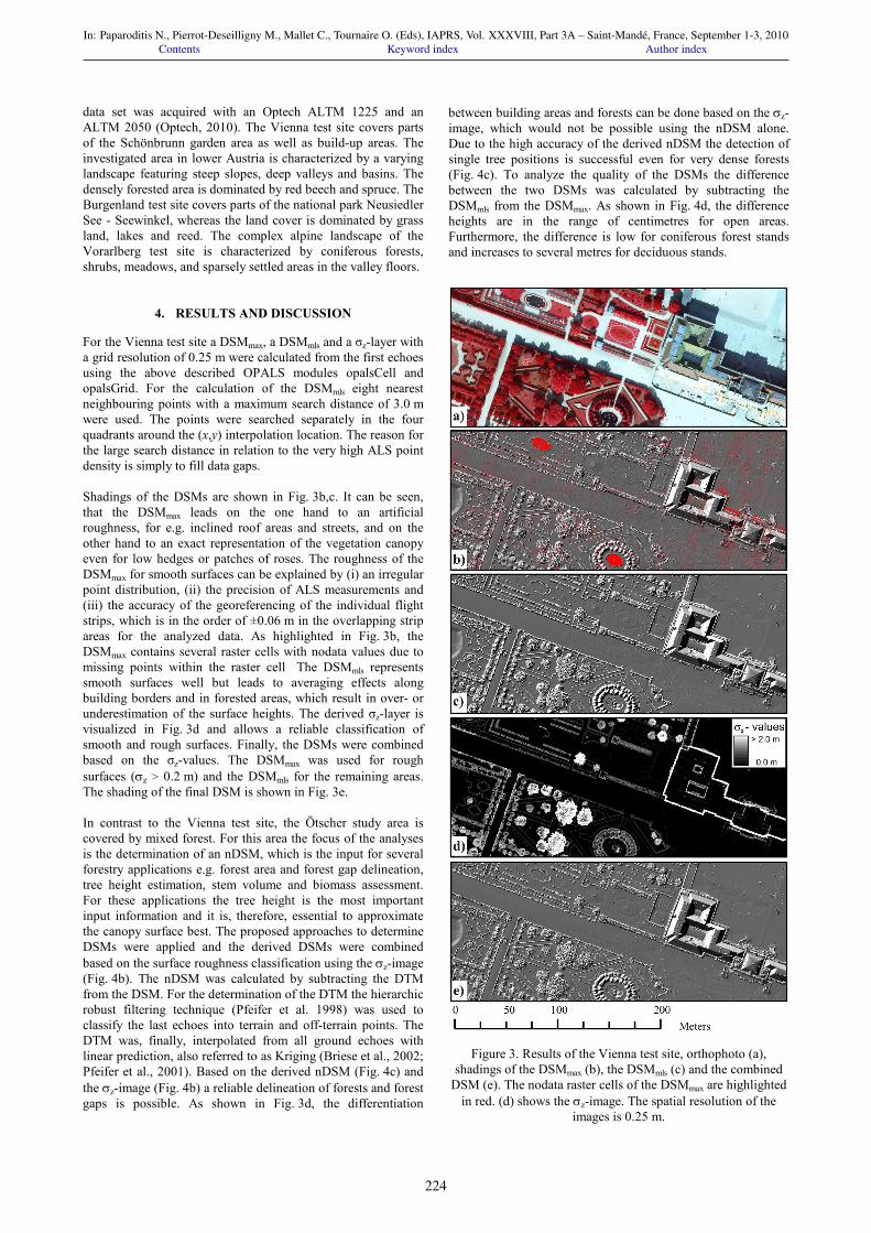
For the Vienna test site a DSMmax, a DSMmls and a σz-layer with a grid resolution of 0.25 m were calculated from the first echoes using the above described OPALS modules opalsCell and opalsGrid. For the calculation of the DSMmls eight nearest neighbouring points with a maximum search distance of 3.0 m were used. The points were searched separately in the four quadrants around the (x,y) interpolation location. The reason for the large search distance in relation to the very high ALS point density is simply to fill data gaps. Shadings of the DSMs are shown in Fig. 3b,c. It can be seen, that the DSMmax leads on the one hand to an artificial roughness, for e.g. inclined roof areas and streets, and on the other hand to an exact representation of the vegetation canopy even for low hedges or patches of roses. The roughness of the DSMmax for smooth surfaces can be explained by (i) an irregular point distribution, (ii) the precision of ALS measurements and (iii) the accuracy of the georeferencing of the individual flight strips, which is in the order of ±0.06 m in the overlapping strip areas for the analyzed data. As highlighted in Fig. 3b, the DSMmax contains several raster cells with nodata values due to missing points within the raster cell The DSMmls represents smooth surfaces well but leads to averaging effects along building borders and in forested areas, which result in over- or underestimation of the surface heights. The derived σz-layer is visualized in Fig. 3d and allows a reliable classification of smooth and rough surfaces. Finally, the DSMs were combined based on the σz-values. The DSMmax was used for rough surfaces (σz > 0.2 m) and the DSMmls for the remaining areas. The shading of the final DSM is shown in Fig. 3e. In contrast to the Vienna test site, the Ötscher study area is covered by mixed forest. For this area the focus of the analyses is the determination of an nDSM, which is the input for several forestry applications e.g. forest area and forest gap delineation, tree height estimation, stem volume and biomass assessment. For these applications the tree height is the most important input information and it is, therefore, essential to approximate the canopy surface best. The proposed approaches to determine DSMs were applied and the derived DSMs were combined based on the surface roughness classification using the σz-image (Fig. 4b). The nDSM was calculated by subtracting the DTM from the DSM. For the determination of the DTM the hierarchic robust filtering technique (Pfeifer et al. 1998) was used to classify the last echoes into terrain and off-terrain points. The DTM was, finally, interpolated from all ground echoes with linear prediction, also referred to as Kriging (Briese et al., 2002; Pfeifer et al., 2001). Based on the derived nDSM (Fig. 4c) and the σz-image (Fig. 4b) a reliable delineation of forests and forest gaps is possible. As shown in Fig. 3d, the differentiation

between building areas and forests can be done based on the σz-image, which would not be possible using the nDSM alone. Due to the high accuracy of the derived nDSM the detection of single tree positions is successful even for very dense forests (Fig. 4c). To analyze the quality of the DSMs the difference between the two DSMs was calculated by subtracting the DSMmls from the DSMmax. As shown in Fig. 4d, the difference heights are in the range of centimetres for open areas. Furthermore, the difference is low for coniferous forest stands and increases to several metres for deciduous stands.

Figure 3. Results of the Vienna test site, orthophoto (a), shadings of the DSMmax (b), the DSMmls (c) and the combined

DSM (e). The nodata raster cells of the DSMmax are highlighted in red. (d) shows the σz-image. The spatial resolution of the

images is 0.25 m.


224

Figure 4. Results of the Ötscher test site. (a) orthophoto adapted from © www.bing.com/maps; (b) σz-image; (c) nDSM derived from the combined DSM minus the DTM; (d) difference model

(DSMmax – DSMmls). The spatial resolution of the images is 0.50 m.

As the ALS data acquisition was carried out under leaf-off conditions and, consequently, several first echoes were reflected from stems or branches within the deciduous tree crowns, the moving planes interpolation leads to a significant underestimation of the surface heights. For the test site Vorarlberg the available ALS data have low point density, which increases the probability to smooth the DSMmls surface. This can clearly be seen in the shadings of the DSMmax and the DSMmls in Fig. 5b,c and in the building and vegetation profiles shown in Fig. 5e. Considerable smoothing effects of the DSMmls occur along the building border (cp. the building in the right part of the figure) and within the forest. Using the DSMmax (Fig. 5b) instead of the DSMmls (Fig. 5c) for rough surfaces improves the accuracy of the final DSM and decreases these smoothing effects. However, with decreasing point densities the amount of nodata values of the calculated DSMmax increases (cp. Fig. 5b). To fill these data gaps the DSMmls was used. Due to the irregular point distribution of the used laser scanner (saw tooth pattern), the DSMmax appears to be rather rough even for smooth and sloped open areas (see Fig. 5b,c).

Figure 5. Illustration of DSM calculations based on (b) the highest point within a defined raster cell (DSMmax) and (c)

moving planes interpolation (DSMmls). In (b) the nodata cells of the DSMmax are highlighted in red. In (d) an nDSM is shown.

The profiles in (e) illustrate the smoothing effects of the moving planes interpolation for a forest (P1) and for a building (P2).

The spatial resolution of the CIR orthophoto (a) is 0.25 m, those of the DSMs and the nDSM 1.0 m.

For such irregular point distributions it is suggested to search the k-nn points, which are used for the moving planes interpolation, separately in the four quadrants around the (x,y) interpolation location in order to avoid extrapolation effects. The combination of both DSMs depending on the σz-values minimizes this effect as far as possible. The derived nDSM is shown in Fig. 5d. For the test site Neusiedler See the difference between the DSMmax and the DSMmls is substantial for reed areas (cp. Fig. 6). Reed is one of the dominant plants in this region and it is of great importance for their ecosystems. Therefore, the underestimation of the reed surface in the order of 1.0 to 1.5 m, as shown in Fig. 6d, would constrain e.g. biodiversity analyses (i.e. determination of the horizontal and vertical distribution of reed). Based on the applied combined DSM calculation even small geometric structures in reed (i.e. linear structure) can be detected, as shown in Fig. 6b, which was not possible using the DSMmls alone.


225

Figure 6. Illustration of DSM calculations for a reed covered area. (a) orthophoto, (b) shading of the land cover dependent

DSM, (c) difference DSM (DSMmax - DSMmls) and (d) profile of both DSMs (red dots - DSMmax; blue dots - DSMmls).

5. CONCLUSIONS

The proposed methodology for deriving high precision DSMs uses surface roughness information to combine DSMs, which are calculated based (i) on the highest echo within a raster cell and (ii) on moving planes interpolation (MLS). The interpolation methods are not new, but the important aspect is that the DSM should be derived using different algorithms, based on the land cover class. The interpolation methodology is thus chosen on the basis of surface roughness, where rough areas correspond to low and high vegetation and to surface jump edges. Surface roughness was selected, because it discriminates between street, house roofs, and open areas on the one hand, and strongly vegetated surfaces on the other hand. In this way, improved DSMs are obtained, which are better for visualization on the one hand, featuring simultaneously sharp house edges and smooth roofs, and which are better applicable for forestry applications, on the other hand, featuring reduced canopy height underestimation and improved possibilities for single tree positioning. Different applications pose different demands on DSMs, and as far as possible, they should be integrated into one surface, which fulfils those different requirements. Not only the application, but also the object properties, e.g. with respect to the sampling distance, call for different surface interpolation techniques. The approach and its implementation presented here are more general than the examples presented. Nonetheless, also the straightforward choice of the model based on a roughness threshold provided improved results.

Extensions in future will analyse the effects of the assumed σz-threshold of 0.2 m on the derived DSM. The discriminatory power of surface roughness for specific land cover class groups will have to be investigated. Furthermore, more land cover classes (proxies of land cover classes) will be considered, e.g. water surfaces with their specific surface interpolation requirements (e.g. moving least squares, maximal values per cell, triangulation, etc.). Also the full waveform parameters of echo width and cross section will be exploit for land cover classification.

6. ACKNOWLEDEGEMENTS

This study was partly done within the project LASER-WOOD (822030) which is funded by the Klima- und Energiefonds in the framework of the program NEUE ENERGIEN 2020 and within the project TransEcoNet that is implemented through the CENTRAL EUROPE Program co-financed by the ERDF. The EO data are provided by the private management of Schönbrunn Palace (member of the Christian Doppler-Laboratory), the Amt der Niederösterreichischen Landesregierung, Gruppe Baudirektion, Abteilung Vermessung und Geoinformation, the Landesvermessungsamt Feldkirch, and by the company RIEGL.

7. REFERENCES

Briese C., Pfeifer N., Dorninger P., 2002. Applications of the Robust Interpolation for DTM Determination. International Archives of Photogrammetry and Remote Sensing, Graz, Austria, Vol. XXXIV, Part 3A, pp. 55-61. Fan, Q., Efrat, A., Koltun, V., Krishnan, S., Venkatasubramanian, S., 2005. Hardware-assisted Natural Neighbor Interpolation. In Proc. 7th Workshop on Algorithm Engineering and Experiments (ALENEX), Vancouver, British Columbia, Canada, pp. 13. Lancaster, P., and Šalkauskas, K., 1990. Curve and Surface Fitting: An Introduction. 3rd ed. Academic Press. Mandlburger G., Otepka J., Karel W., Wagner W., Pfeifer N., 2009. Orientation And Processing of Airborne Laser Scanning Data (opals) - Concept And First Results of a Comprehensive ALS Software. ISPRS Workshop Laserscanning `09, IAPRS, Paris, France, Vol. XXXVIII, Part 3/W8, pp. 55-60. OPALS - Orientation and Processing of Airborne Laser Scanning Data, 2010. http://www.ipf.tuwien.ac.at/opals/ opals_docu/index.html, last accessed February 2010. Optech, 2010. http://www.optech.on.ca/ Pfeifer N., Köstli A., Kraus K., 1998. Interpolation and Filtering of Laser Scanner Data-Implementation and First Results. International Archives of Photogrammetry, Remote Sensing and Spatial Information Sciences, Columbus, Ohio, USA, Vol. XXXII, Part 3/1, pp. 153-159. Pfeifer N., Stadler P., Briese C., 2001. Derivation of Digital Terrain Models in the SCOP++ Environment. OEEPE Workshop on Airborne Laserscanning and Interferometric SAR for Detailed Digital Elevation Models. Stockholm, Sweden, pp. 13. Python, 2010. Python programming language. http://www.python.org/ Riegl, 2010. Airborne Scanner data sheets. http://www.riegl.com/ Sithole G., Vosselman G., 2004. Experimental comparison of filter algorithms for bare-Earth extraction from airborne laser scanning point clouds. ISPRS Journal of Photogrammetry & Remote Sensing 59(1-2), pp. 85-101.


226

Documents

LAND COVER DEPENDENT DERIVATION OF DIGITAL …