Ladder studies of gapless quantum spin liquids: Spin-Bosemetal and SU(2)-invariant Majorana spin liquids

Thesis by

Hsin-Hua Lai

In Partial Fulfillment of the Requirements

for the Degree of

Doctor of Philosophy

California Institute of Technology

Pasadena, California

2012

(Defended May 9 2012)

c© 2012

Hsin-Hua Lai

All Rights Reserved

ii

To my family and fiancee, for unconditional support, and to all my friends.

iii

Acknowledgements

First of all, I would like to express my gratitude to the committee members: Lesik Motrunich,

Gil Refael, Michael Cross, and Nai-Chang Yeh for being willing to take the time to be my

thesis defense committee, read the thesis, and give comments. Especially I want to thank

my thesis advisor, Lesik Motrunich, who has always been very encouraging, patient, and

willing to spend lots of time discussing with me. This dissertation would not have been pos-

sible without his guidance. I also would like to thank Gil Refael for sharing his insights and

views now and then, which always brings different perspectives to thinking about physics.

I also would like to thank my officemates Tony Lee and Tiamhock Tay for sharing new

ideas and chatting about things related to the real world. To my Caltech friends—Chang-Yu

Hou, Eyal Kenig, Shankar Iyer, Shu-Ping Lee, Kun Woo Kim, Liyan Qiao, Jason Alicea,

and many others in ACT—I want to thank you for enriching my life here at Caltech.

Finally, I am most grateful to my family for their support; to my fiancee U Shan Chen

for love, patience, and always encouraging me to keep going forward.

iv

Abstract

The recent experimental realizations of spin-1/2 gapless quantum spin liquids in two-

dimensional triangular lattice organic compounds EtMe3Sb[Pd(dmit)2]2 and κ-(ET)2Cu2(CN)3

have stimulated the investigation of the gapless spin liquid theories. The models in dimen-

sions greater than one (D > 1) usually involve multispin interactions, such as ring ex-

change interactions, that are difficult to study, while effective gauge theory descriptions are

not well-controlled to give reliable physics information. Driven by the need for a systematic

and controlled analysis of such phase, such models on ladders are seriously studied. This

thesis first focuses on such ladder models. We propose that the gapless spin liquid phase

can be accessed from a two-band interacting electron model by metal-Mott insulator phase

transition. We use Bosonization analysis and weak-coupling Renormalization Group to fur-

ther study the gapless spin liquid state in the presence of Zeeman magnetic fields or orbital

magnetic fields. Several new exotic gapless spin liquids with dominant spin nematic cor-

relations are predicted. In such a ladder spin liquid, we also consider the impurity effects.

We conclude that the local energy textures and oscillating spin susceptibilities around the

impurities are nontrivial and can be observed in the experiments. We then shift our focus

to another theoretical candidate, an SU(2)-invariant spin liquid with Majorana excitations,

which can also qualitatively explain the experimental phenomenology. We construct an ex-

actly solvable Kitaev-type model realizing the long-wavelength Majorana spin liquid state

and study its properties. We find that the state has equal power-law spin and spin-nematic

correlations and behaves nontrivially in the presence of Zeeman magnetic fields. Finally,

we realize such Majorana spin liquid states on a two-leg ladder and further explore their

stability. We conclude the states can be stable against short-range interactions and gauge

field fluctuations.

v

Contents

Acknowledgements iv

Abstract v

1 Introduction 1

1.1 Gapless spin liquid material: κ-(ET)2Cu2(CN)3 . . . . . . . . . . . . . . . 4

1.1.1 Crystal and electronic structures of κ-(ET)2Cu2(CN)3 . . . . . . . . 4

1.1.2 Spin liquid in κ-(ET)2Cu2(CN)3 . . . . . . . . . . . . . . . . . . . 5

1.2 Gapless spin liquid material: EtMe3Sb[Pd(dmit)2]2 . . . . . . . . . . . . . 8

1.2.1 Crystal and electronic structures of EtMe3Sb[Pd(dmit)2]2 . . . . . . 8

1.2.2 Spin liquid in EtMe3Sb[Pd(dmit)2]2 . . . . . . . . . . . . . . . . . 9

1.3 Overview of thesis . . . . . . . . . . . . . . . . . . . . . . . . . . . . . . 13

2 Preliminaries 15

2.1 Bosonization primer . . . . . . . . . . . . . . . . . . . . . . . . . . . . . . 15

2.2 Weak-coupling renormalization group (RG) and current algebra . . . . . . 21

2.3 Spin Bose-metal theory on the zigzag strip . . . . . . . . . . . . . . . . . . 26

2.3.1 SBM via Bosonization of gauge theory . . . . . . . . . . . . . . . 28

2.3.2 SBM by Bosonizing interacting electrons . . . . . . . . . . . . . . 30

2.3.3 Fixed-point theory of the SBM phase . . . . . . . . . . . . . . . . 32

2.4 Original Kitaev model on the honeycomb lattice . . . . . . . . . . . . . . . 33

3 Two-band electronic metal and neighboring spin liquid (spin Bose-metal) on a

zigzag strip with longer-ranged repulsion 38

vi

3.1 Weak coupling analysis of t1− t2 model with extended repulsion: Stabiliz-

ing C2S2 metal . . . . . . . . . . . . . . . . . . . . . . . . . . . . . . . . 40

3.1.1 Setup for two-band electron system . . . . . . . . . . . . . . . . . 40

3.1.2 Weak coupling renormalization group . . . . . . . . . . . . . . . . 43

3.1.3 Fixed point for stable C2S2 phase . . . . . . . . . . . . . . . . . . 43

3.1.4 Numerical studies of the flows . . . . . . . . . . . . . . . . . . . . 44

3.1.5 Examples of phase diagrams with C2S2 metal stabilized by ex-

tended interactions . . . . . . . . . . . . . . . . . . . . . . . . . . 45

3.1.5.1 Weak coupling phase diagram for potential Eq. (3.31) . . 46

3.1.5.2 Weak coupling phase diagram for potential Eq. (3.31)

truncated at the 4th neighbor . . . . . . . . . . . . . . . 48

3.2 Weak-to-intermediate coupling: Phases out of C2S2 upon increasing inter-

action . . . . . . . . . . . . . . . . . . . . . . . . . . . . . . . . . . . . . 49

3.2.1 Harmonic description of the C2S2 phase . . . . . . . . . . . . . . . 49

3.2.2 Mott insulator driven by Umklapp interaction. Intermediate cou-

pling procedure out of the C2S2 . . . . . . . . . . . . . . . . . . . 52

3.2.2.1 Instability out of C1[ρ−]S2 driven by spin-charge cou-

pling W . . . . . . . . . . . . . . . . . . . . . . . . . . 53

3.2.2.2 Instability out of C1[ρ+]S0 driven by Umklapp H8 . . . 54

3.2.3 Numerical results . . . . . . . . . . . . . . . . . . . . . . . . . . . 54

3.2.3.1 Intermediate coupling phase diagram for model with po-

tential Eq. (3.31) . . . . . . . . . . . . . . . . . . . . . . 54

3.2.3.2 Intermediate coupling phase diagram for model with po-

tential Eq. (3.31) truncated at the 4th neighbor . . . . . . 59

3.3 Summary and discussion . . . . . . . . . . . . . . . . . . . . . . . . . . . 59

3.A Derivation of ∆[cos (4θρ+)] and ∆[cos (2ϕρ−)] in C2S2 phase . . . . . . . 62

4 Effects of Zeeman field on a spin Bose-metal phase 65

4.1 Electrons on a two-leg zigzag strip in a Zeeman field: Weak coupling ap-

proach . . . . . . . . . . . . . . . . . . . . . . . . . . . . . . . . . . . . . 67

vii

4.2 Transition to Mott insulator: SBM phase . . . . . . . . . . . . . . . . . . . 74

4.3 Observables in the SBM in Zeeman field . . . . . . . . . . . . . . . . . . . 77

4.4 Nearby phases out of the SBM in the field . . . . . . . . . . . . . . . . . . 81

4.4.1 Phases when w↑12 is relevant . . . . . . . . . . . . . . . . . . . . . 81

4.4.2 Phases when both w↑12 and w↓12 are relevant . . . . . . . . . . . . . 83

4.4.2.1 w↑12 > 0, w↓12 > 0 . . . . . . . . . . . . . . . . . . . . . 84

4.4.2.2 w↑12 < 0, w↓12 < 0 . . . . . . . . . . . . . . . . . . . . . 85

4.4.2.3 w↑12 > 0, w↓12 < 0 . . . . . . . . . . . . . . . . . . . . . 85

4.4.2.4 w↑12 < 0, w↓12 > 0 . . . . . . . . . . . . . . . . . . . . . 86

4.5 Discussion . . . . . . . . . . . . . . . . . . . . . . . . . . . . . . . . . . . 87

5 Insulating phases of electrons on a zigzag strip in the orbital magnetic field 90

5.1 Weak coupling approach to electrons on a zigzag strip with orbital field . . 91

5.2 Observables in the Mott-insulating phase in orbital field . . . . . . . . . . . 98

5.3 Spin-gapped phases in orbital field . . . . . . . . . . . . . . . . . . . . . . 103

5.3.1 λσ11 < 0, λσ22 > 0, λσ12 > 0 . . . . . . . . . . . . . . . . . . . . . . 104

5.3.2 λσ11 > 0, λσ22 < 0, λσ12 > 0 . . . . . . . . . . . . . . . . . . . . . . 104

5.3.3 λσ11, λσ22 > 0, λσ12 < 0 . . . . . . . . . . . . . . . . . . . . . . . . . 104

5.3.4 λσ11, λσ22 < 0, λσ12 > 0 . . . . . . . . . . . . . . . . . . . . . . . . . 105

5.3.5 λσ12 < 0 and either λσ11 < 0 or λσ22 < 0 . . . . . . . . . . . . . . . . 106

5.4 Discussion . . . . . . . . . . . . . . . . . . . . . . . . . . . . . . . . . . . 106

6 Effects of impurities in spin Bose-metal phase on a two-leg triangular strip 108

6.1 Nonmagnetic impurities in the spin Bose-metal on the ladder . . . . . . . . 109

6.1.1 Nonmagnetic defects treated as perturbations . . . . . . . . . . . . 111

6.1.2 Physical calculations of oscillating susceptibility and bond textures

in the fixed-point theory of semi-infinite chains . . . . . . . . . . . 114

6.1.3 Other situations with impurities . . . . . . . . . . . . . . . . . . . 116

6.1.3.1 Weakly coupled semi-infinite systems . . . . . . . . . . 116

6.1.3.2 Spin-12

impurity coupled to a semi-infinite system . . . . 117

viii

6.1.3.3 Two semi-infinite systems coupled symmetrically to a

spin-12

impurity . . . . . . . . . . . . . . . . . . . . . . 117

6.2 Conclusions . . . . . . . . . . . . . . . . . . . . . . . . . . . . . . . . . . 118

6.A One-mode theory on a semi-infinite chain . . . . . . . . . . . . . . . . . . 119

6.B Calculations in a fixed-point theory of a semi-infinite system with pinned

θσ+(0), ϕσ−(0), and ϕρ−(0) . . . . . . . . . . . . . . . . . . . . . . . . . . 120

7 SU(2)-invariant Majorana spin liquid with stable parton Fermi surfaces in an

exactly solvable model 123

7.1 SU(2)-invariant Majorana spin liquid with stable Fermi surfaces . . . . . . 125

7.2 Correlation functions . . . . . . . . . . . . . . . . . . . . . . . . . . . . . 129

7.2.1 Long wavelength analysis . . . . . . . . . . . . . . . . . . . . . . 131

7.2.2 Exact numerical calculation . . . . . . . . . . . . . . . . . . . . . 134

7.3 Majorana spin liquid in the Zeeman field . . . . . . . . . . . . . . . . . . . 136

7.4 Discussion . . . . . . . . . . . . . . . . . . . . . . . . . . . . . . . . . . . 140

8 Majorana spin liquids on a two-leg ladder 142

8.1 Gapless Majorana orbital liquid (MOL) on a two-leg ladder . . . . . . . . . 144

8.1.1 Fixed-point theory of Majorana orbital liquid and observables . . . 148

8.1.2 Stability of Majorana orbital liquid . . . . . . . . . . . . . . . . . 152

8.2 Gapless SU(2)-invariant Majorana spin liquid (MSL) on the two-leg ladder 155

8.3 Discussion . . . . . . . . . . . . . . . . . . . . . . . . . . . . . . . . . . . 159

8.A Stability of gapless U(1) matter against Z2 gauge field fluctuations in (1+1)D161

8.B Fixed-point theory and observables in the SU(2) Majorana spin liquid . . . 166

8.C Zeeman magnetic field effects on the SU(2) Majorana spin liquid . . . . . . 173

8.D SU(2) Majorana spin liquid with time reversal breaking (TRB) . . . . . . . 175

Bibliography 177

ix

Chapter 1

Introduction

At an early stage of introduction to interacting spin systems, students are taught that at low

temperature the spin states mostly tend to “align” or “anti-align” with each other to form

ordered states: the ferromagnet or the anti-ferromagnet. The phase transition to such states

involves breaking of symmetries and can be described by phenomenological Ginzburg-

Landau theory. However, quantum fluctuations can break the above naive classical picture

and the spin states can even remain disordered down to zero temperature. One such ex-

ample is that of the one-dimensional (1D) anti-ferromagnetic spin-1/2 Heisenberg chain,

which has no long range order and its ground state possesses power law correlations [1].

Another famous example is the 1D spin-1 antiferromagnetic chain proposed by Haldane

[2] to have a disordered ground state with a gap to excitations.

Another way to suppress magnetic long range order is “frustration” due to the geometry

of lattice. Take a simple anti-ferromagnetic Ising model on a square and on a triangle for

instance, Fig. 1.1. Due to the geometry of these two plaquettes, the ground state on the

square is the Neel anti-ferromagnet. However, in the ground state of the triangle the spins

cannot be arranged to simultaneously minimize all the interactions, which suppresses the

magnetic order. The situation in the second case is what we call the frustration. Besides,

low lattice dimension typically increases the frustration and also the quantum fluctuations.

Hence, there is a possibility of quantum spin liquids(QSL) [3, 4, 5] in a low-dimensional

highly frustrated lattice.

Focusing on the lattice dimension greater than one, we now know theoretically there

are many different kinds of spin liquids. Gapped topological spin liquids [6, 7, 8, 9, 10,

1

Figure 1.1: Schematic pictures of antiferromagnetic Ising spin model on a square and atriangle. For the spins on a square, each spin is antiparallel with its neighbor to end up withtwo exact ground states. However, all three spins on a triangle cannot be antiparallel andinstead of the two ground states mandated by the Ising symmetry (up and down), there aresix ground states. This is the simplest example of frustration. The red lines denote the axison which the spins are parallel

11, 12, 13, 14] are quite well-understood and have been theoretically shown to exist in

model systems. However, none of these theoretically well-understood gapped spin liq-

uids are realized in the experiment. On the other hand, even though “gapless” spin liquids

[3, 13, 11] are less understood theoretically, there have been series of experimental re-

ports of promising gapless spin liquid states in two-dimensional(2D) organic compounds

EtMe3Sb[Pd(dmit)2]2 and κ-(ET)2Cu2(CN)3 [15, 16, 17, 18, 19, 20, 21, 22, 23, 24, 25, 26].

The details of these two spin liquid materials will be discussed in Chapters 1.1 and 1.2. The

striking features of such compounds are the absence of long range magnetic order in the

zero temperature limit, but the presence of finite spin susceptibilities, “metal-like” linear

temperature dependent specific heat and thermal conductivity even though they are in Mott

insulating phase.

One theoretical proposal suggests the state with Gutzwiller-projected spinon Fermi sea

wave function [27, 28] in a 2D quantum spin-1/2 Heisenberg model with four-site ring

exchange terms. This proposal leads to a theory of spinons coupled to U(1) gauge fields.

However, there is no well-controlled theoretical access to such phase in 2D. From a the-

oretical point of view, it is difficult to analyze a model involving multi-spin interactions

2

(four-site ring exchange) and challenging to analyze gauge theory. From the perspective

of numerics, most of the numerical tools cannot be used or do not give reliable unbiased

information in such highly frustrated lattices. For example, the exact diagonalization (ED)

studies are restricted to very small sizes, variational Monte Carlo (VMC) results are biased

by the input wavefunctions, quantum Monte Carlo (QMC) fails due to the sign problem in

such highly frustrated lattices, and density matrix renormalization group (DMRG) is able

to give reliable unbiased information but suffers from the growth of entanglement in 2D

and can not be applied in a large 2D lattice.

Driven by the needs for further understandings of the interesting phase, the ladder ver-

sions of such theoretical model have been studied [29, 30, 31, 32, 33, 34] and the ladder

descendant of the gapless spin liquid state has been found and dubbed spin Bose-metal

(SBM). Focusing on the SBM phase, in Chapters 3–5 we explore several experimentally

motivated questions in the two-leg ladder. Since experiments suggest that the gapless spin

liquid phase sit in the insulating side near the metal-Mott insulator phase transition line, in

Chapter 3 we propose to access the SBM phase from a two-band Hubbard-type model. In

Chapters 4–5 we consider separately the effects of Zeeman magnetic field and the effects

of orbital magnetic field on the SBM. In Chapter 6 we consider the effects of impurities on

the SBM.

For a smoking gun experiment for the proposal of spinon Fermi sea state, Katsura

et al. [35] suggest that in the presence of orbital magnetic field, the flux of the spinon U(1)

gauge field couples to the orbital field and leads to the observation of a finite thermal Hall

conductance if the deconfined Fermionic spinons indeed exist and is responsible for the

observed thermal current. However, the experiment reports no observation of the thermal

Hall effect due to the deconfined spinons [23]. One theoretical possible explanation is the

U(1) gauge fluctuations are suppressed due to some partial pairing of spinons [36, 37, 32],

but it is not clear yet.

Searching for other theoretical proposals, Biswas et al. suggested a SU(2)-invariant

gapless spin liquid with spinful Majorana excitations. The striking feature of the spin liquid

state is that the external magnetic field has no orbital coupling to the SU(2) spin rotation-

invariant Fermion bilinears that can give rise to a transverse thermal conductivity. Hence,

3

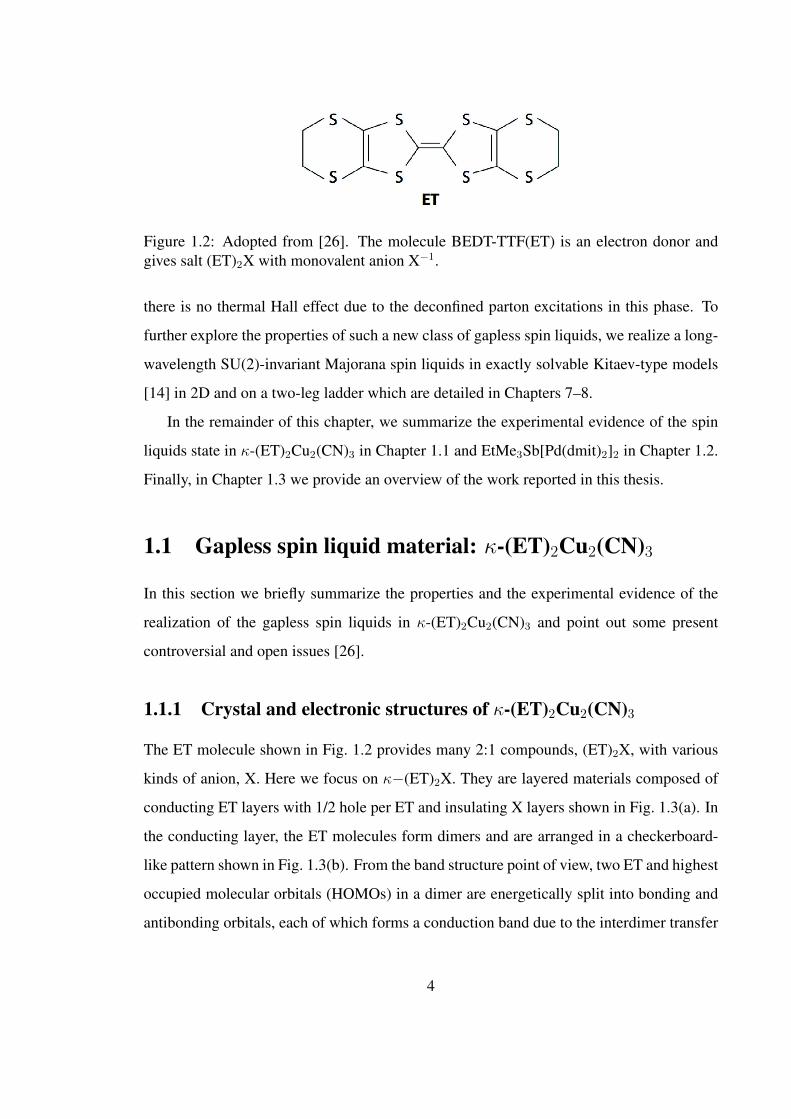
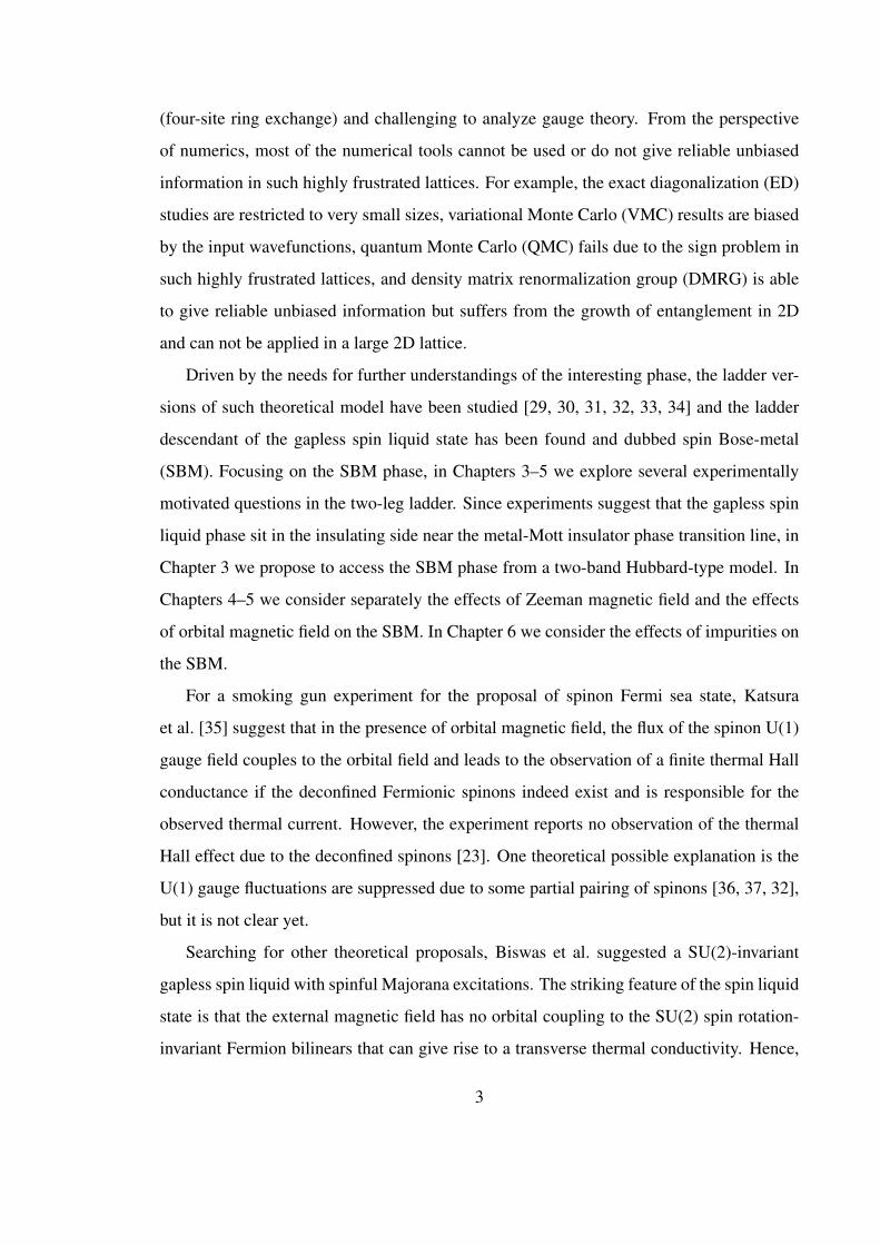
Figure 1.2: Adopted from [26]. The molecule BEDT-TTF(ET) is an electron donor andgives salt (ET)2X with monovalent anion X−1.

there is no thermal Hall effect due to the deconfined parton excitations in this phase. To

further explore the properties of such a new class of gapless spin liquids, we realize a long-

wavelength SU(2)-invariant Majorana spin liquids in exactly solvable Kitaev-type models

[14] in 2D and on a two-leg ladder which are detailed in Chapters 7–8.

In the remainder of this chapter, we summarize the experimental evidence of the spin

liquids state in κ-(ET)2Cu2(CN)3 in Chapter 1.1 and EtMe3Sb[Pd(dmit)2]2 in Chapter 1.2.

Finally, in Chapter 1.3 we provide an overview of the work reported in this thesis.

1.1 Gapless spin liquid material: κ-(ET)2Cu2(CN)3

In this section we briefly summarize the properties and the experimental evidence of the

realization of the gapless spin liquids in κ-(ET)2Cu2(CN)3 and point out some present

controversial and open issues [26].

1.1.1 Crystal and electronic structures of κ-(ET)2Cu2(CN)3

The ET molecule shown in Fig. 1.2 provides many 2:1 compounds, (ET)2X, with various

kinds of anion, X. Here we focus on κ−(ET)2X. They are layered materials composed of

conducting ET layers with 1/2 hole per ET and insulating X layers shown in Fig. 1.3(a). In

the conducting layer, the ET molecules form dimers and are arranged in a checkerboard-

like pattern shown in Fig. 1.3(b). From the band structure point of view, two ET and highest

occupied molecular orbitals (HOMOs) in a dimer are energetically split into bonding and

antibonding orbitals, each of which forms a conduction band due to the interdimer transfer

4

(a) (b) (c)

Figure 1.3: Adopted from [26]. (a) Side view of the layer structure of κ-(ET)2Cu2(CN)3.We can see the conducting ET layers are separated by the nonmagnetic cation layers, X.(b) Top view of the conducting ET layer. The ET molecules form dimers and are arrangedin a checkerboard-like pattern. (c) The intradimer couplings are much stronger than theinterdimer couplings and each dimer can be treated as a single unit. Hence, the ET dimersin (b) can be simplified to the triangular lattice model with each site occupied by exactlyone electron.

integrals. The two bands are well separated so that the relevant band to the hole filling is

the antibonding band, which is half-filled with one hole accommodated by one antibonding

orbital. The dimer arrangement is modeled to an isosceles-triangular lattice characterized

by two interdimer transfer integrals, t and t′, Fig. 1.3(c), of the order of 50 meV, whose

anisotropy, t′/t, is 1.06 or 0.80 to 0.83 according to the tight-binding calculation of molec-

ular orbital or first-principles calculation. [38, 39] The thermal transport experiment [40]

indicates that the Mott-insulating compound κ-(ET)2Cu2(CN)3 sits very close to the metal-

Mott insulator transition line with a very small Mott charge gap, about 200 K. Because of

the very small gap, we call κ-(ET)2Cu2(CN)3 a weak Mott insulator. We remark that due

to the small charge gap, the theoretical quantum spin model should include the high-order

spin interactions (i.e., 3-site or 4-site ring exchange terms) besides the usual Heisenberg

interactions.

1.1.2 Spin liquid in κ-(ET)2Cu2(CN)3

Figure 1.4(a) shows the temperature dependence of the magnetic susceptibility with the

core diamagnetism subtracted [15]. κ-(ET)2Cu2(CN)3 has no anomaly down to the low-

est temperature measured, 2 K, but does have a broad peak, which is well fitted to the

5

(a) (b)

Figure 1.4: Adopted from [26]. (a) Temperature dependences of spin susceptibilities of κ-(ET)2Cu2(CN)3 and κ-(ET)2Cu(CN)2Cl. The solid lines represent the results of the seriesexpansion of the triangular-lattice Heisenberg model. (b) 1H NMR spectra of single crystalsof κ-(ET)2Cu2(CN)3 (left) and κ-(ET)2Cu(CN)2Cl (right) under magnetic fields appliedperpendicular to the conducting layer

triangular-lattice Heisenberg model with an exchange interaction of J ∼ 250 K [15]. The

magnetism is further probed by 1H nuclear magnetic resonance (NMR) measurements.

Figure 1.4(b) shows the single-crystal 1H NMR spectra for κ-(ET)2Cu(CN)2Cl and κ-

(ET)2Cu2(CN)3 under the magnetic field applied perpendicular to the conduction layer.

The line shape at high temperatures comes from the fact that the nuclear dipole interaction

is sensitive to the field direction relative to the molecular orientation, which is different be-

tween the two systems. The material κ-(ET)2Cu(CN)2Cl shows a clear line splitting below

27 K, indicating a commensurate antiferromagnetic ordering, whose moment is estimated

at 0.45 µB per an ET dimer by separate 13C NMR studies [41, 42, 43]. On the other hand,

the spectra of κ-(ET)2Cu2(CN)3 show neither distinct broadening nor splitting, which indi-

cates the absence of long-range magnetic ordering at least down to 32 mK which is 4 orders

of magnitude lower than the exchange coupling J. The result points to the first realization of

a quantum spin liquid in κ-(ET)2Cu2(CN)3 due to the strong spin frustration on the nearly

equilateral triangular lattice.

6

(a) (b)

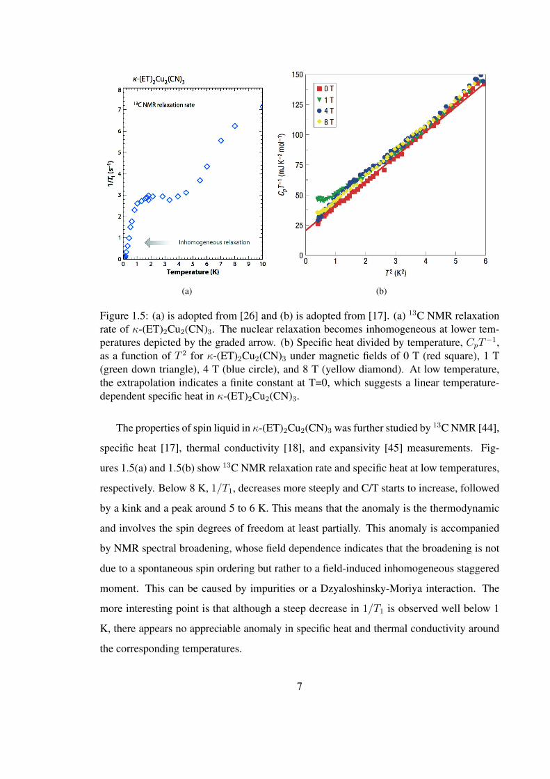
Figure 1.5: (a) is adopted from [26] and (b) is adopted from [17]. (a) 13C NMR relaxationrate of κ-(ET)2Cu2(CN)3. The nuclear relaxation becomes inhomogeneous at lower tem-peratures depicted by the graded arrow. (b) Specific heat divided by temperature, CpT−1,as a function of T 2 for κ-(ET)2Cu2(CN)3 under magnetic fields of 0 T (red square), 1 T(green down triangle), 4 T (blue circle), and 8 T (yellow diamond). At low temperature,the extrapolation indicates a finite constant at T=0, which suggests a linear temperature-dependent specific heat in κ-(ET)2Cu2(CN)3.

The properties of spin liquid in κ-(ET)2Cu2(CN)3 was further studied by 13C NMR [44],

specific heat [17], thermal conductivity [18], and expansivity [45] measurements. Fig-

ures 1.5(a) and 1.5(b) show 13C NMR relaxation rate and specific heat at low temperatures,

respectively. Below 8 K, 1/T1, decreases more steeply and C/T starts to increase, followed

by a kink and a peak around 5 to 6 K. This means that the anomaly is the thermodynamic

and involves the spin degrees of freedom at least partially. This anomaly is accompanied

by NMR spectral broadening, whose field dependence indicates that the broadening is not

due to a spontaneous spin ordering but rather to a field-induced inhomogeneous staggered

moment. This can be caused by impurities or a Dzyaloshinsky-Moriya interaction. The

more interesting point is that although a steep decrease in 1/T1 is observed well below 1

K, there appears no appreciable anomaly in specific heat and thermal conductivity around

the corresponding temperatures.

7

Final key issue on the nature of this spin liquid material is whether the spin liquid is

gapped. The experimental observations are still controversial. The specific heat points to

the presence of a finite γ value (indication of linear temperature dependent Cp) comparable

to that in the metallic phase down to at least 0.3–0.4 K, below which the nuclear Schottky

contribution becomes overwhelming [17]. The thermal conductivity measurements indi-

cate that the thermal excitation is gapped below 0.46 K [18]. The 13C NMR relaxation

rate shows a power-law temperature dependence with an exponent of 3/2; although, the nu-

clear relaxation is inhomogeneous at low temperature [44]. They are all inconsistent with

each other. More systematic experimental studies are needed to provide more significant

information of such spin liquid phase in κ-(ET)2Cu2(CN)3.

1.2 Gapless spin liquid material: EtMe3Sb[Pd(dmit)2]2

In this section we summarize the properties and the experimental evidence of the gapless

spin liquid state in EtMe3Sb[Pd(dmit)2]2 and discuss some present controversial and open

issues. [26]

1.2.1 Crystal and electronic structures of EtMe3Sb[Pd(dmit)2]2

The Pd(dmit)2 salts, (Cation) [Pd(dmit)2]2, exhibit 2D layer structures and have the follow-

ing features:

1. Pd(dmit)2 units are strongly dimerized with an eclipsed overlapping mode to form

[Pd(dmit)2]−2 with one negative charge. The degree of dimerization is stronger than

that in the κ−type ET salts.

2. In contrast to the κ−type ET salts, the dimer units show face-to-face stacking, Fig. 1.6(a).

3. Within the 2D conduction layer, the dimer units form a quasi-triangular lattice, Fig. 1.6(b).

Figure 1.6(a) shows the side view of the 3D crystal structure of EtMe3Sb[Pd(dmit)2]2.

The unit cell contains two crystallographically equivalent conduction layers interrelated by

a glide plane. They are separated from each other by the insulating cation layer.

8

(a) (b)

Figure 1.6: Adopted from [26]. (a) Side view of the layer structure ofEtMe3Sb[Pd(dmit)2]2. We can see the conducting Pd(dmit)2 molecule layers are separatedby the nonmagnetic cation layers. (b) Top view of the Pd(dmit)2 layer and the Pd(dmit)2

molecules are strongly dimerized and are arranged in a checkerboard-like pattern. The in-tradimer couplings are much stronger than the interdimer couplings and thus each dimer canbe treated as a single unit and in the end can be simplified to the triangular lattice modelwith three unequal transfer integrals, t, t′, and t′′. Since it is very close to an isosceles-triangular lattice, we treat t′ ' t′′.

The electronic structure around the Fermi level can be described by the dimer-based

tight-binding approximation. The dimers, [Pd(dmit)2]−2 form a scalene-triangular lattice

where they are connected by three unequal transfer integrals, t, t′, and t′′ in Fig. 1.6(b).

However, they are very close to an isosceles-triangular lattice and thus we treat t′ ' t′′.

From quantum chemistry calculation, t′/t ' 0.92 for EtMe3Sb[Pd(dmit)2]2 and is so frus-

trated that a spin liquid phase can be realized.

1.2.2 Spin liquid in EtMe3Sb[Pd(dmit)2]2

Figure 1.7(a) shows the temperature dependence of the magnetic susceptibility with the

core diamagnetism subtracted. EtMe3Sb[Pd(dmit)2]2 has no anomaly down to the lowest

temperature measured, 5 K, but have a broad peak, which is well fitted to the triangular-

lattice-Heisenberg model with an exchange interaction of J ∼ 250 K [21]. The magnetism

is further probed by 13C NMR measurements. Figure 1.7(b) shows the single-crystal 13C

NMR spectra for EtMe3Sb[Pd(dmit)2]2, which do not show significant broadening down

to 19.4 mK [22]. Although very slight gradual broadening is observed, the width is much

9

(a) (b)

Figure 1.7: Adopted from [26]. (a) Temperature dependence of the spin susceptibilityof randomly oriented samples of EtMe3Sb[Pd(dmit)2]2. Solid curves show the result ofthe [7/7] Pade approximants for the high-temperature expansion of the regular-triangularantiferromagnetic spin-1/2 system with J=220 and 250 K. (b) 13C NMR spectra from 272K to 19.4 mK for randomly oriented samples of EtMe3Sb[Pd(dmit)2]2. It is clear there isno further splitting of the peak, which indicates no formation of long-range magnetic order.

smaller than the scale of the hyperfine coupling constant of the 13C sites. This clearly

indicates that there is no spin ordering or freezing down to the lowest temperature. Because

this temperature is smaller than 0.01% of J, thermal fluctuations are negligible, and the

absence of spin ordering or freezing should be attributed to quantum fluctuations.

As for the issue of whether the spin liquid state in EtMe3Sb[Pd(dmit)2]2 is gapless,

the experimental observations are still controversial but it seems the gapless spin liquid

is more favored. Figure 1.8(a) shows the previous studies of the spin-lattice relaxation

rate 1/T1 curve fitted by the stretched exponential function. The stretching exponents β

indicates homogeneity of the system. The β value being smaller than unity means that the

system is inhomogeneous. The temperature dependence of β indicated that inhomogeneity

is enhanced from approximately 20 K and reaches maximum around 1 K. A sharp drop

of 1/T1 below 1 K suggest a continuous phase transition that involves symmetry breaking

10

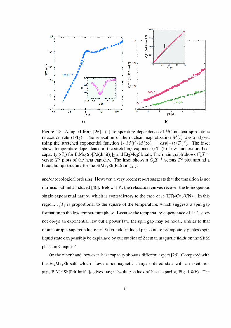
(a) (b)

Figure 1.8: Adopted from [26]. (a) Temperature dependence of 13C nuclear spin-latticerelaxation rate (1/T1). The relaxation of the nuclear magnetization M(t) was analyzedusing the stretched exponential function 1- M(t)/M(∞) = exp[−(t/T1)β]. The insetshows temperature dependence of the stretching exponent (β). (b) Low-temperature heatcapacity (Cp) for EtMe3Sb[Pd(dmit)2]2 and Et2Me2Sb salt. The main graph shows CpT−1

versus T 2 plots of the heat capacity. The inset shows a CpT−1 versus T 2 plot around abroad hump structure for the EtMe3Sb[Pd(dmit)2]2.

and/or topological ordering. However, a very recent report suggests that the transition is not

intrinsic but field-induced [46]. Below 1 K, the relaxation curves recover the homogenous

single-exponential nature, which is contradictory to the case of κ-(ET)2Cu2(CN)3. In this

region, 1/T1 is proportional to the square of the temperature, which suggests a spin gap

formation in the low temperature phase. Because the temperature dependence of 1/T1 does

not obeys an exponential law but a power law, the spin gap may be nodal, similar to that

of anisotropic superconductivity. Such field-induced phase out of completely gapless spin

liquid state can possibly be explained by our studies of Zeeman magnetic fields on the SBM

phase in Chapter 4.

On the other hand, however, heat capacity shows a different aspect [25]. Compared with

the Et2Me2Sb salt, which shows a nonmagnetic charge-ordered state with an excitation

gap, EtMe3Sb[Pd(dmit)2]2 gives large absolute values of heat capacity, Fig. 1.8(b). The

11

(a) (b)

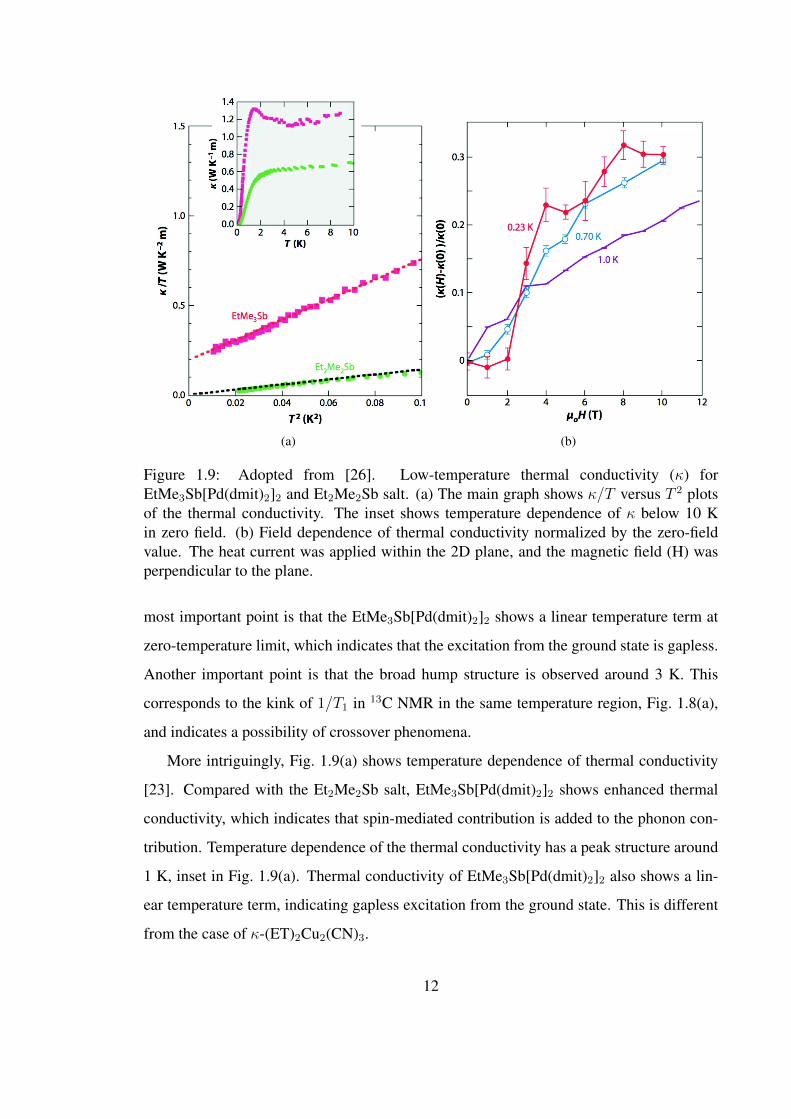
Figure 1.9: Adopted from [26]. Low-temperature thermal conductivity (κ) forEtMe3Sb[Pd(dmit)2]2 and Et2Me2Sb salt. (a) The main graph shows κ/T versus T 2 plotsof the thermal conductivity. The inset shows temperature dependence of κ below 10 Kin zero field. (b) Field dependence of thermal conductivity normalized by the zero-fieldvalue. The heat current was applied within the 2D plane, and the magnetic field (H) wasperpendicular to the plane.

most important point is that the EtMe3Sb[Pd(dmit)2]2 shows a linear temperature term at

zero-temperature limit, which indicates that the excitation from the ground state is gapless.

Another important point is that the broad hump structure is observed around 3 K. This

corresponds to the kink of 1/T1 in 13C NMR in the same temperature region, Fig. 1.8(a),

and indicates a possibility of crossover phenomena.

More intriguingly, Fig. 1.9(a) shows temperature dependence of thermal conductivity

[23]. Compared with the Et2Me2Sb salt, EtMe3Sb[Pd(dmit)2]2 shows enhanced thermal

conductivity, which indicates that spin-mediated contribution is added to the phonon con-

tribution. Temperature dependence of the thermal conductivity has a peak structure around

1 K, inset in Fig. 1.9(a). Thermal conductivity of EtMe3Sb[Pd(dmit)2]2 also shows a lin-

ear temperature term, indicating gapless excitation from the ground state. This is different

from the case of κ-(ET)2Cu2(CN)3.

12

Field dependence of thermal conductivity of EtMe3Sb[Pd(dmit)2]2, however, suggest

another kind of excitation, Fig 1.9(b). A steep increase above approximate 2 T is observed

below 1 K, which implies that some spin-gap-like excitations are present at low tempera-

tures, along with the gapless excitation indicated by the T-linear term. As mentioned earlier,

there is a field-induced phase transition in low temperature in this spin liquid material [46].

Such field dependence of thermal conductivity of EtMe3Sb[Pd(dmit)2]2 is likely to pro-

vide the excitation information of the field-induced phase but not the intrinsic properties of

the completely gapless spin liquid state. Possible explanation is that there exists an exotic

spin liquid state induced by the Zeeman magnetic field with part of the Fermi surface is

gapped out due to pairing, which is detailed in Chapter 4. The theoretical scenarios are

still debating and more experiments are required to uncover the mysterious physics in this

material.

1.3 Overview of thesis

In Chapter 2 we introduce the techniques we mainly use in this thesis such as Bosoniza-

tion and weak-coupling Renormalization Group (RG). The effective theory of SBM is also

briefly summarized, which is the foundation for the studies of SBM in Chapters 3–6. We

also provide a concise introduction to the original Kitaev model on the honeycomb lattice

and focus on the relevant properties of the model. The same idea can be directly applied to

construct other Kitaev-type models that we study in Chapters 7–8

In Chapter 3 we start from a two-band Hubbard-type model with longer-ranged repul-

sions on a two-leg triangular ladder and access to the SBM phase by metal-Mott insulator

phase transition. We propose a schematic phase diagram in this model in which the SBM

phase can be realized in the intermediate coupling regime.

In Chapter 4 we consider the Zeeman magnetic field effect on the SBM phase. We

conjecture there should be a new exotic quantum spin liquid phase out of SBM. In this

phase, only one species of spinons are paired up while the other species of spinons still have

an intact Fermi surface. In Chapter 5 we study the orbital magnetic field effect on the SBM

phase. We start from a two-band Hubbard-type model on the two-leg triangular ladder and

13

we conclude that the combination of the orbital magnetic field and interactions provides a

mechanism to drive metal-insulator transition already at weak coupling. According to RG

analysis, the SBM phase is fragile to the orbital magnetic field in this model.

For further understanding of other effects on the SBM phase, in Chapter 6 we study

the impurity effects on the SBM and find the formation of bond-energy textures around

impurities and nontrivial increasing oscillating spin susceptibility around impurities, which

can be detected in Knight shift measurements in NMR.

In Chapter 7 we realize the long-wavelength SU(2) Majorana spin liquids (MSL) in a

Kitaev-type model with broken time-reversal symmetry and lattice inversion symmetry to

avoid discussing possible instability. Unlike usual SU(2)-invariant spin liquids, there are

three species of Fermions that carry Sz = ±1 and 0. We find that SU(2) MSL possess

equal power-law spin and spin-nematic correlation functions. In the presence of Zeeman

magnetic fields, we conjecture a nontrivial half-magnetization plateau phase in which spin

excitations are gapful while there remains spinless gapless excitations that still produce

metal-like thermal properties.

Finally, in Chapter 8 we realize the Majorana liquids [including Majorana orbital liquid

(MOL) using only orbital degrees of freedom and SU(2) MSL using both spin and orbital

degrees of freedom] on a two-leg ladder in a Kitaev-type model to systematically study its

stability in a well-controlled RG analysis. We conclude such Majorana liquids are stable

against weak local perturbations and Z2 gauge fields fluctuations.

14

Chapter 2

Preliminaries

In this chapter we introduce the techniques that we use in this thesis. In Chapter 2.1 we

introduce the bosonization, a powerful tool of reformulating fermions in terms of Bosons,

in a 1D spinless free electron system [47, 48]. In Chapter 2.2 we first introduce the concepts

of weak-coupling RG and use current algebra [49] to derive the RG equations algebraically

in 1D electron systems with weak interactions. We summarize the SBM theory [29] in

Chapter 2.3 which is the foundation for the ladder studies of SBM in Chapters 3–6. In

Chapter 2.4 we introduce the original Kitaev model on the honeycomb lattice [14] concisely

whose spirits can be directly applied to construct other exactly solvable Kitaev-type models

that we study in Chapters 7–8.

2.1 Bosonization primer

In this review, we follow closely [47] to introduce the Bosonization technique. Let us

consider the Hamiltonian for non-interacting spinless electrons hopping on a 1D lattice,

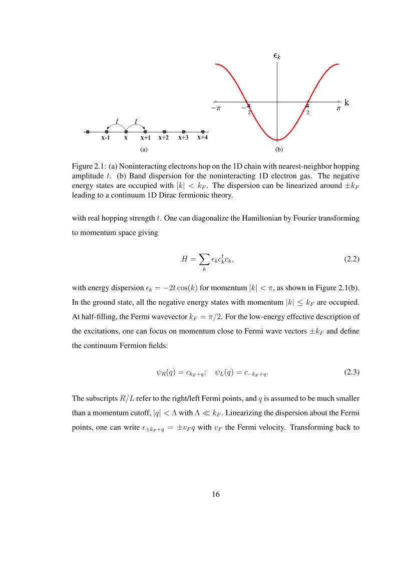
Fig. 2.1(a)

H = −t∑x

[c†(x)c(x+ 1) + H.c.

], (2.1)

15

tt

x x+1 x+2 x+3 x+4x-1

(a) (b)

Figure 2.1: (a) Noninteracting electrons hop on the 1D chain with nearest-neighbor hoppingamplitude t. (b) Band dispersion for the noninteracting 1D electron gas. The negativeenergy states are occupied with |k| < kF . The dispersion can be linearized around ±kFleading to a continuum 1D Dirac fermionic theory.

with real hopping strength t. One can diagonalize the Hamiltonian by Fourier transforming

to momentum space giving

H =∑k

εkc†kck, (2.2)

with energy dispersion εk = −2t cos(k) for momentum |k| < π, as shown in Figure 2.1(b).

In the ground state, all the negative energy states with momentum |k| ≤ kF are occupied.

At half-filling, the Fermi wavevector kF = π/2. For the low-energy effective description of

the excitations, one can focus on momentum close to Fermi wave vectors ±kF and define

the continuum Fermion fields:

ψR(q) = ckF+q; ψL(q) = c−kF+q. (2.3)

The subscriptsR/L refer to the right/left Fermi points, and q is assumed to be much smaller

than a momentum cutoff, |q| < Λ with Λ� kF . Linearizing the dispersion about the Fermi

points, one can write ε±kF+q = ±vF q with vF the Fermi velocity. Transforming back to

16

real space, one can define fields

ψP (x) =1√L

∑|q|<Λ

eiqxψP (q), (2.4)

which vary slowly on the scale of the lattice spacing with P = R/L. The above equation

is equivalent to expanding the usual lattice electron fields in terms of continuum fields,

c(x) ∼ ψR(x)eikF x + ψL(x)e−ikF x. (2.5)

In terms of the continuum fields, the effective low-energy Hamiltonian takes the form,

H =∫dxH, with Hamiltonian density,

H = vF

[ψ†R(−i∂x)ψR − ψ†L(−i∂x)ψL

], (2.6)

which describes a 1D relativistic Dirac particle.

Consider a particle/hole excitation about the right Fermi point, where an electron is

removed from an occupied state with k < kF and placed into an unoccupied state with k+

q > kF . For small momentum change q, the energy of this excitation is ωq = vF q. Together

with the negative momentum excitations about the left Fermi point, this linear dispersion

relation is identical to that for phonons in 1D. The method of bosonization exploits this

similarity by introducing a phonon displacement field θ, to describe this linearly dispersing

density wave. Let us consider a Jordan-Wigner transformation which replace the electron

operator, c(x), by a boson operator with so-called Jordan-Wigner “string” attached to the

boson operator,

c(x) = O(x)b(x) ≡ eiπ∑x′<x n(x′)b(x), (2.7)

with n(x) = c†(x)c(x), the number operator. This transformation of exchanging Fermions

for bosons is a special feature of 1D. The boson operators can be (approximately) decom-

17

posed in terms of an amplitude and a phase,

b(x)→ √ρeiϕ. (2.8)

We now imagine going to the continuum limit, focusing on scales long compared to the

lattice spacing. In this limit, we decompose the total density as, ρ(x) = ρ0 + ρ, where the

mean density, ρ0 = kF/π, and ρ is an operator measuring the fluctuations in the density.

The density and phase are canonically conjugate quantum variables satisfying

[ϕ(x), ρ(x′)] = iδ(x− x′). (2.9)

Now we introduce a phonon-like displacement field, θ(x), via ρ(x) = ∂xθ(x)/π. Then the

full density takes the form, πρ(x) = kF + ∂xθ and the above commutation relations are

satisfied if one takes

[ϕ(x), θ(x′)] = iπΘ(x− x′). (2.10)

Here Θ(x) denotes the heavyside step function. Note that ∂xϕ/π is the momentum conju-

gate to θ.

As described above, the goal of the bosonization is to replace the original low-energy

continuum Fermions by the phonon-like bosons in 1D. To this end, we can start from the

effective bosonized Hamiltonian density which describes the 1D density wave (phonon-

like) takes the form:

H =v

2π

[g(∂xϕ)2 + g−1(∂xθ)

2]. (2.11)

This Hamiltonian describes a wave propagating at velocity v. The equations of motions

can be obtained using the commutation relation above, ∂2t θ = (gv)2∂2

xθ, and similarly

for ϕ. In the “noninteracting” case, one can clearly equate v with the Fermi velocity vF .

The additional dimensionless parameter g can be determined as follows. Let us consider a

1D phonon-like system. A small variation in density ρ will lead to a change in the energy,

18

E = ρ2/2κ, where κ = ∂ρ/∂µ = ∂ρ/∂EF . Since ∂xθ = πρ, one can obtain κ = g/πv. For

a non-interacting electron system, ∂ρ/∂µ = κ = n(EF ) = 1/πv, so that g = 1. However,

in the presence of short-ranged interactions between the electrons, the Hamiltonian density

expression remains valid but the values of both g and v should be renormalized away from

the non-interacting free electron gas. Therefore, this Hamiltonian would then describe a

(spinless) Luttinger liquid.

To identify the relation between the usual electron operator c(x) and the Boson fields,

one can consider first the Bose operator, b ∼ eiϕ, which removes unit charge at x. Note that

eiϕ(x) = eiπ∫ x−∞ dx′P (x′), (2.12)

where P = ∂xϕ/π is the momentum conjugate to θ. Since the momentum operator is the

generator of translations in θ, this creates a kink in θ of height π centered at position x-

which corresponds to a localized unit of charge since the density is ρ = ∂xθ/π. Besides,

the attached Jordan-Wigner string in the bosonic language can be viewed as

O(x) = eiπ∑x′<x n(x′) ' eiπ

∫ x ρ(x′) = ei(kF x+θ), (2.13)

where in the second equality we used the fact that ρ = ρ0 + ρ. Hence, we can see the

string operator carries momentum kF and the resulting fermionic operator Oeiϕ should be

identified as the “right-moving” continuum Fermi field, ψR. Similarly, we can introduce

Boson field replacing the left-moving continuum Fermi field, ψL. The correct bosonized

form for the continuum electron operators are

ψP (x) = eiφP (x); φP = ϕ+ Pθ, (2.14)

with P = R/L = ±. According to Eqs. (2.9)–(2.10), the chiral boson field φP satisfy the

so-called Kac-Moody commutation relations:

[φP (x), φP (x′)] = iPπsign(x− x′), (2.15)

[φR(x), φL(x′)] = iπ. (2.16)

19

These commutation relations can be used to show that ψR and ψL anti-commute.

Let us now express the bosonized Hamiltonian density in terms of the chiral boson field.

First, let us consider the “noninteracting” system. We define the right- and left-moving

boson densities as

nP =P

2π∂xφP , (2.17)

which gives the total density nR + nL = ∂xθ/π = ρ. The bosonized Hamiltonian density

becomes

H = πvF[n2R + n2

L

]. (2.18)

These chiral boson density can be expressed in term of the chiral (continuum) electron

operators as,

nP =: ψ†PψP :≡ ψ†PψP − 〈ψ†PψP 〉. (2.19)

In the noninteracting limit, the bosonized Hamiltonian decouples into right and left moving

sectors as the case in usual continuum Fermi fields.

The advantage of bosonization is that we can easily take short-ranged electron interac-

tions into account. For example, the density-density interaction, V (x) = Un(x)n(x + 1),

can be added to the original Hamiltonian. Expansion in terms of continuum fermions us-

ing Eq. (2.5) gives three terms which conserve the momentum: Two chiral terms of the

form (ψ†PψP )2, and a term mixing right/left-moving fermions of the form ψ†RψRψ†LψL.

Under bosonization, the two chiral terms become of the “quadratic” form proportional to

(∂xφP )2, and can be treated to renormalize the Fermi velocity in Eq. (2.18). The other term

mixing left/right sectors also becomes a “quadratic” term proportional to (∂xφR)(∂xφL) ∼

(∂xθ)2 − (∂xϕ)2, and renormalize the Luttinger parameter g away from one. For repulsive

interaction, one finds g < 1 while g > 1 for attractive interaction. Therefore, we can see

the power of the bosonization technique is that the “quartic” fermion interactions under

bosonization can still give “quadratic” terms which can be treated analytically.

20

2.2 Weak-coupling renormalization group (RG) and cur-

rent algebra

The starting point for the weak-coupling RG analysis is writing down the effective low-

energy Hamiltonian of relativistic Dirac fermions after linearizing the spectrum around the

Fermi points similar to the discussions in Chapter 2.1. The kinetic energy takes the form,

H0 =∫dxH0, with Hamiltonian density,

H0 =∑i,α

vαi

[ψ†Riα(−i∂x)ψRiα − ψ†Liα(−i∂x)ψLiα

], (2.20)

with i labeling the different bands and α labeling different species of fermions (usually

labeling spin index, but can be more general). The Euclidean action, written as a space-

time integral of the Lagrangian density, is

S =

∫dτdxL0, (2.21)

L0 =∑Piα

i∂τψPiα +H0, (2.22)

with P = R/L, and τ denoting imaginary time. The partition function can be expressed as

a coherent state Grassmann path integral,

Z =

∫[Dψ][Dψ]e−S(ψ,ψ). (2.23)

We can follow standard RG steps as described by Shankar [50]. First integrating out field

ψ(k, ω) with momentum k lying in the interval Λ/b < |k| < Λ, with rescaling parameter

b > 1. We then perform the rescaling procedure which returns the cutoff to its original

value:

x→ bx; τ → bτ ; ψ → b−1/2ψ. (2.24)

21

The action remains invariant after the scaling, and the non-interacting theory above is at a

RG “fixed point”.

Away from the noninteracting limit, the interactions can scatter right-moving Fermions

into left-moving Fermions and vice-versa. For example, if we consider the usual on-site

density–density repulsion, a.k.a Hubbard repulsion, after expansion in terms of continuum

fermion fields, it contains terms of the quartic form as ψ†P1ψP2ψ†P3ψP4, with P1, P2, P3,

P4 = R/L. In Euclidean space-time (1+1)D, such quartic terms are again “invariant”

under rescaling procedure in RG and are marginal.

In order to know if such quartic terms are marginally relevant, strictly marginal, or

marginally irrelevant, we need to consider the one-loop contribution in RG analysis. Ref-

erence [50] already detailed the standard procedure for analyzing RG at tree level and at

one-loop corrections, which we will skip here. Instead, we will introduce the so-called

“current-algebra” to “algebraically” calculate the one-loop RG correction. Most of the pro-

cedures are listed clearly in the Appendix in [49]. Below we will use a 1D Hubbard model

at half-filling to illustrate how the current algebra works.

Let us consider a 1D spinful electron hopping system at half-filling with the Hamilto-

nian similar to Eq. (2.1) but now there is a spin index called α. The band spectrum is the

same to Fig. 2.1(b) but now there are two degenerate bands. After linearizing around the

Fermi points, the effective low-energy, noninteracting Hamiltonian density is

H0 = v∑α

[ψ†Rα(−i∂x)ψRα − ψ†Lα(−i∂x)ψLα

]. (2.25)

We can easily take interactions into account as perturbations. After expansion in terms of

continuum fermions, the allowed four-fermion interactions are highly constrained by the

symmetries of the system. In this model, these terms should be invariant under spin SU(2)

rotation, parity transformation, time-reversal, and spatial translation. A convenient way to

write down the interactions is by introducing the current operators as

JP = ψ†PαψPα; ~JP = 12ψ†Pα(~σ)αβψPβ , (2.26)

IP = ψPαεαβψPβ; ~IP = 12ψPα(ε~σ)αβψPβ, (2.27)

22

with P = R/L and repeated indices mean summation. JP and IP transform as scalars and

~JP and ~IP transform as vectors under SU(2) rotation. Note that since there is only one band

in this model, ~IP are actually zero. However, the expressions above are more general and

are readily generalized to other models with multibands.

With the current operators above, the allowed four-fermion interactions can be written

in a concise form as

−Hint = wρJRJL + wσ ~JR · ~JL + uρ

[I†RIL + H.c.

]. (2.28)

We can now algebraically calculate the one-loop RG. The fermions in Euclidean space

obey the operator product expansion (OPE) [51, 52]

ψRα(x, τ)ψ†Rβ(0, 0) ∼ δαβ2πz

+O(1), (2.29)

ψLα(x, τ)ψ†Lβ(0, 0) ∼ δαβ2πz∗

+O(1), (2.30)

where z = vτ−ix, with v the Fermi velocity. The OPE are valid when two points (x, τ) and

(0, 0) are brought close together, as replacement within correlation functions. In principle,

if we consider any product of the current operators, the operators products can be qualita-

tively considered as some generalized Wick contractions. As an example, we consider the

product J jRJkR. Performing all possible contraction gives

J jR(z)JkR(0) ∼ : ψ†Rα(z)ψRβ(z) :: ψ†Rγ(0)ψRε(0) :1

4σjαβσ

kγε

∼[−(−1

2πz

)(1

2πz

)δαεδβγ +

δβγ2πz

: ψ†RαψRε :

+δαε2πz

: ψRβψ†Rγ : + : ψ†RαψRβψ

†RγψRε :

]1

4σjαβσ

kγε

∼ 1

2(2πz)2δjk +

1

2πziεjklJ lR +O(1)

∼ 1

2πziεjklJ lR, (2.31)

where above we used σjσk = δjk + iεjklσl, and in the last line we dropped all the irrelevant

terms. Skipping the derivations for other OPE, we list all the relevant results at half-filling

23

caseJR(z)IR(0) ∼ −1

πzIR; JL(z)IL(0) ∼ −1

πz∗IL,

JR(z)I†R(0) ∼ 1πzI†R; JL(z)I†L(0) ∼ 1

πz∗I†L,

IRI†R(0) ∼ − 2

πzJR; IL(z)I†L(0) ∼ −2

2πz∗JL,

J jL(z)JkL(0) ∼ 12πz∗

iεjklJ lL.

(2.32)

The RG equations can be obtained from the equations above. In the Euclidean space,

the action is SE =∫dxdτH, withH = H0 +Hint, and the partition function is

Z =

∫[dψ][dψ]e−SE . (2.33)

To perform the RG, the exponential is expanded to quadratic order in Hint. For example,

let us examine a term which takes the form

u2ρ

2

∫z,w

⟨(I†R(z)IL(z) + H.c.)(I†L(w)IR(w) + H.c.)

⟩' u2

ρ

∫z,w

4

2π(z − w)

−4

2π(z∗ − w∗)JRJL. (2.34)

Following the steps in [49], we choose a short-distance (high-momentum) cutoff a in space,

but none in imaginary time. For a rescaling factor b, we must then perform the integral

I =

∫a<|x|<ba

dx

∫ ∞−∞

dτ1

(2π)2(v2τ 2 + x2)=

ln b

2πv(2.35)

over the relative coordinates (x, τ). Eq. (2.34) becomes

−4u2

ρ

πvln b

∫z

JRJL, (2.36)

which when re-exponentiated, for b = edl, gives the RG equation for wρ as

wρ = −8u2

ρ

πv, (2.37)

with O ≡ ∂O/∂l, and l is logarithm of the length scale.

We can follow similar steps to derive the complete RG equations for this 1D electron

24

model at half-filling,

wρ = − 8

πvu2ρ, (2.38)

wσ = − 1

2πvw2σ, (2.39)

uρ = − 2

πvwρuρ. (2.40)

As an example, we consider the on-site Hubbard model with

HU = U∑x

n↑(x)n↓(x). (2.41)

After expanding the interaction in terms of the continuum field, we find the bare values of

the couplings,

wρ(l = 0) = −U2

; wσ(l = 0) = 2U ; uρ(l = 0) = −U4. (2.42)

Once we have the RG equations, Eqs. (2.38)–(2.40), and the initial conditions (bare cou-

plings), Eq. (2.42), we can qualitatively analyze the phase diagram at weak coupling. First,

let us consider repulsive interaction, U > 0. After plugging the initial conditions, Eq. (2.42)

into Eqs. (2.38)–(2.40), qualitatively wσ keeps decreasing to become marginally irrelevant

while uρ becomes divergent ( uρ → −∞) and relevant to drive wρ to diverge eventually

(wρ → −∞). The coupling uρ corresponds to coupling strength of the (I†RIL+H.c.), which

in Fermion language is the Umklapp interaction coming from commensurability. Hence,

for U > 0, the phase with relevant uρ corresponds to a “Mott insulator”.

On the other hand, if we consider attractive interaction, U < 0, qualitatively the Umk-

lapp couplings uρ and wρ quickly become very small under RG and are marginally irrele-

vant, while wσ becomes divergent (wσ → −∞) and relevant. The wσ corresponds to the

interactions which involve the currents, ~JP , defined in Eq. (2.26). From symmetry consid-

erations, since ~JP transform as SU(2) vectors just as spins, such interactions are expected

to affect mainly the spin degrees of freedom (spin sectors). Indeed, the marginally relevant

coupling wσ opens a gap in spin sector and the corresponding phase is the Emery-Luther

25

(a) (b)

Figure 2.2: (a) 2D triangular lattice. (b) The top figure shows the two-leg triangular strip,which can be represented as 1D chain with nearest-neighbor and second-neighbor cou-plings shown in the bottom figure.

liquid. [53]

2.3 Spin Bose-metal theory on the zigzag strip

In this section we follow [29] to provide effective low energy theory for the SBM on the

zigzag chain. In the 2D triangular lattice, Fig. 2.2(a), one approach to spin liquids is to

decompose the spin operators in terms of an SU(2) spinor—the fermionic spinons:

~S =1

2f †α~σαβfβ ; f †αfα = 1 . (2.43)

In the mean field one assumes that the spinons do not interact with one another and are

hopping freely on the 2D lattice. For the present model in this thesis the mean field Hamil-

tonian would have the spinons hopping in zero magnetic field, and the ground state would

correspond to filling up a spinon Fermi sea. In doing this one has artificially enlarged the

Hilbert space, since the spinon hopping Hamiltonian allows for unoccupied and doubly

occupied sites, which have no meaning in terms of the spin model of interest. It is thus nec-

essary to project back down into the physical Hilbert space for the spin model, restricting

the spinons to single occupancy. This can be readily achieved by the Gutzwiller projection,

where one simply drops all terms in the wavefunction with unoccupied or doubly occupied

26

sites.

The alternate approach to implement the single occupancy constraint is by introducing

a gauge field, a U(1) gauge field in this instance, that is minimally coupled to the spinons

in the hopping Hamiltonian. This then becomes an intrinsically strongly-coupled lattice

gauge field theory. To proceed, it is necessary to resort to an approximation by assuming

that the gauge field fluctuations are weak. In 2D one then analyzes the problem of a Fermi

sea of spinons coupled to a weakly fluctuating gauge field. This problem has a long history

[54, 55, 56, 57, 58, 59, 60, 61, 3], but all the authors have chosen to sum the same class

of diagrams. Within this approximation one can then compute physical spin correlation

functions, which are gauge invariant. It is unclear, however, whether this is theoretically

legitimate, and even less clear whether or not the spin liquid phase thereby constructed

captures correctly the universal properties of a physical spin liquid that can occur for some

spin Hamiltonian.

Fortunately, on the zigzag chain, Fig. 2.2(b), it is possible to employ bosonization to

analyze the quasi-1D gauge theory, as we will detail below. While this still does not give

an exact solution for the ground state of any spin Hamiltonian, with regard to capturing

universal low-energy properties it is controlled. As we will see, the low-energy effective

theory for the SBM phase is a Gaussian field theory, and perturbations about this can be

analyzed in a systematic way to check for stability of the SBM and possible instabilities

into other phases.

As detailed in Chapter 3, the-low energy effective theory for the SBM can also be

obtained by starting with a model of interacting electrons hopping on the zigzag chain,

i.e., a Hubbard-type Hamiltonian. If one starts with interacting electrons, it is possible

to construct the gapped electron excitations in the SBM Mott insulator. Within the gauge

theory approach, the analogous gapped spinon excitations are unphysical, being confined

together with a linear potential. Moreover, within the electron formulation one can access

the metallic phase, and also the Mott transition to the SBM insulator.

27

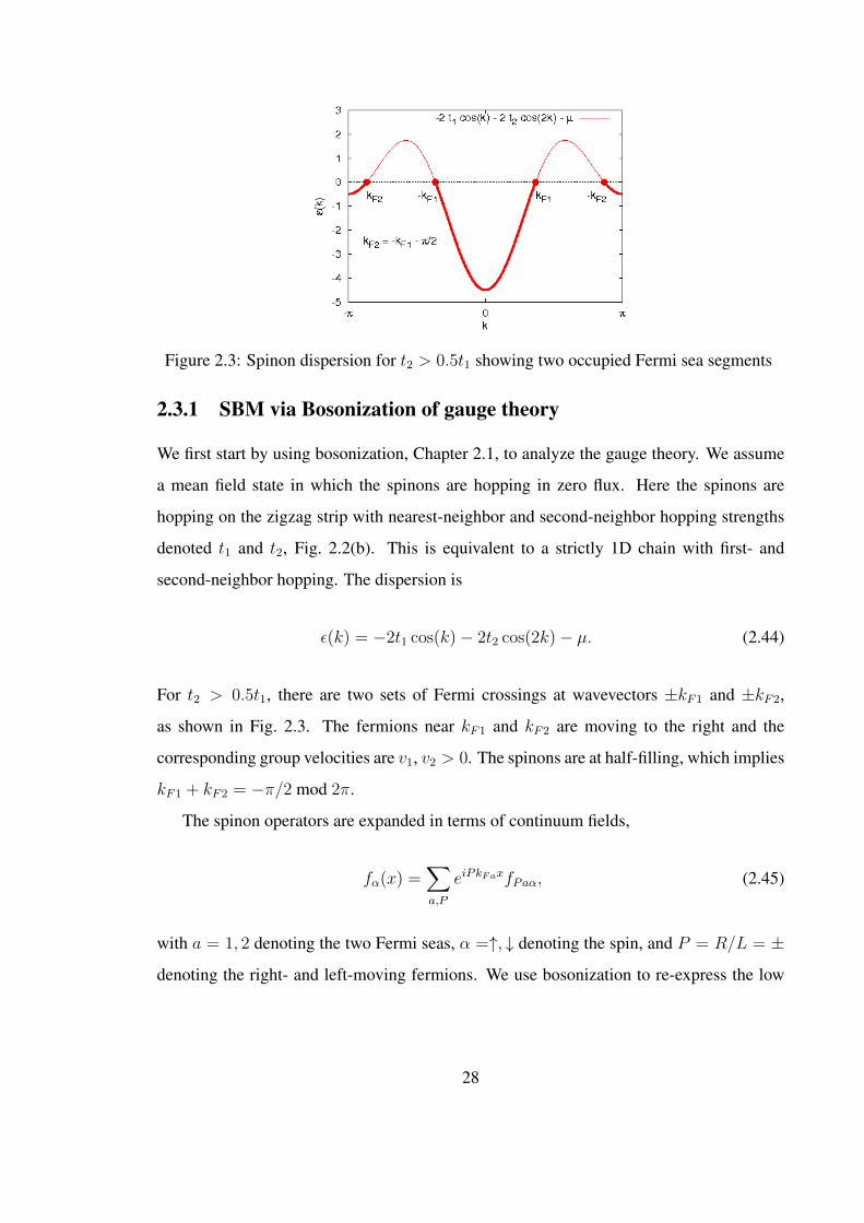
Figure 2.3: Spinon dispersion for t2 > 0.5t1 showing two occupied Fermi sea segments

2.3.1 SBM via Bosonization of gauge theory

We first start by using bosonization, Chapter 2.1, to analyze the gauge theory. We assume

a mean field state in which the spinons are hopping in zero flux. Here the spinons are

hopping on the zigzag strip with nearest-neighbor and second-neighbor hopping strengths

denoted t1 and t2, Fig. 2.2(b). This is equivalent to a strictly 1D chain with first- and

second-neighbor hopping. The dispersion is

ε(k) = −2t1 cos(k)− 2t2 cos(2k)− µ. (2.44)

For t2 > 0.5t1, there are two sets of Fermi crossings at wavevectors ±kF1 and ±kF2,

as shown in Fig. 2.3. The fermions near kF1 and kF2 are moving to the right and the

corresponding group velocities are v1, v2 > 0. The spinons are at half-filling, which implies

kF1 + kF2 = −π/2 mod 2π.

The spinon operators are expanded in terms of continuum fields,

fα(x) =∑a,P

eiPkFaxfPaα, (2.45)

with a = 1, 2 denoting the two Fermi seas, α =↑, ↓ denoting the spin, and P = R/L = ±

denoting the right- and left-moving fermions. We use bosonization to re-express the low

28

energy spinon operators with bosonic fields,

fPaα = ηaαei(ϕaα+Pθaα), (2.46)

with canonically conjugate boson fields:

[ϕaα(x), ϕbβ(x′)] = [θaα(x), θbβ(x′)] = 0, (2.47)

[ϕaα(x), θbβ(x′)] = iπδabδαβΘ(x− x′), (2.48)

where Θ(x) is the heaviside step function and we have introduced Klein factors, the Ma-

jorana fermions {ηaα, ηbβ} = 2δabδαβ , which assure that the spinon fields with different

flavors anticommute with one another.

In this (1+1)D continuum theory, we work in the gauge eliminating spatial components

of the gauge field. The imaginary-time bosonized Lagrangian density is:

L =1

2π

∑aα

[1

va(∂τθaα)2 + va(∂xθaα)2

]+ LA . (2.49)

Here LA encodes the coupling to the slowly varying 1D (scalar) potential field A(x),

LA =1

m(∂xA/π)2 + iρAA , (2.50)

where ρA denotes the total “gauge charge” density,

ρA =∑aα

∂xθaα/π . (2.51)

It is useful to define “charge” and “spin” boson fields,

θaρ/σ =1√2

(θa↑ ± θa↓) , (2.52)

29

and “even” and “odd” flavor combinations,

θµ± =1√2

(θ1µ ± θ2µ) , (2.53)

with µ = ρ, σ. Similar definitions hold for the ϕ fields. The commutation relations for the

new θ, ϕ fields are unchanged.

Integration over the gauge potential generates a mass term,

LA = m(θρ+ − θ(0)ρ+)2 , (2.54)

for the field θρ+ =∑

aα θaα/2. In the gauge theory analysis, we cannot determine the mean

value θ(0)ρ+, which is important for detailed properties of the SBM. However, if we start with

an interacting electron model, one can readily argue that the correct value in the SBM phase

satisfies

4θ(0)ρ+ = π mod 2π . (2.55)

2.3.2 SBM by Bosonizing interacting electrons

The SBM phase can be also accessed via a model of electrons hopping on the zigzag strip.

The details are presented in Chapter 3. In this subsection we briefly summarize the ap-

proach. We assume that the electron hopping Hamiltonian is identical to the spinon mean

field Hamiltonian, with first- and second-neighbor hopping strengths, t1, t2;

H = −∑x

[t1c†α(x)cα(x+ 1) + t2c

†α(x)cα(x+ 2) + H.c.] +Hint . (2.56)

The electrons are taken to be at half-filling. The interaction between the electrons could

be taken as a usual on-site Hubbard repulsion or a longer-ranged repulsive interaction as in

Chapter 3, but we do not need to specify the precise form for what follows.

For t2 < 0.5t1, the electron Fermi sea has only one segment spanning [−π/2, π/2], and

at low energy the model is essentially the same as the 1D Hubbard model. This case is the

30

same as the case we discussed in Chapter 2.2. We know that in this case even an arbitrary

weak repulsive interaction will induce an allowed four-fermion Umklapp term that will be

marginally relevant driving the system into a 1D Mott insulator. The residual spin sector

will be described in terms of the Heisenberg chain, and is expected to be in the gapless

Bethe-chain phase.

On the other hand, for t2 > 0.5t1, the electron band has two Fermi seas as shown in

Fig. 2.3. As in the one-band case, Umklapp terms are required to drive the system into

a Mott insulator. But in this two-band case there are no allowed four-fermion Umklapp

terms. We focus on the allowed eight-fermion Umklapp term which takes the form,

H8 = v8(c†R1↑c†R1↓c

†R2↑c

†R2↓cL1↑cL1↓cL2↑cL2↓ + H.c.) , (2.57)

where we have introduced slowly varying electron fields for the two bands, at the right and

left Fermi points. For repulsive electron interactions we have v8 > 0. This Umklapp term

is strongly irrelevant at weak coupling since its scaling dimension is ∆8 = 4 (each electron

field has scaling dimension 1/2), much larger than the space-time dimension D = 2.

We can bosonize the electrons, cPaα ∼ ei(ϕaα+Pθaα). The eight-fermion Umklapp term

becomes,

H8 = 2v8 cos(4θρ+) , (2.58)

where as before θρ+ =∑

aα θaα/2 and ρe(x) = 2∂xθρ+/π is now the physical slowly

varying electron density. The bosonized form of the noninteracting electron Hamiltonian

is precisely the first part of Eq. (2.49), and one can readily confirm that ∆8 = 4. But

now imagine adding a strong density–density repulsion between the electrons. The slowly

varying contributions, on scales larger than the lattice spacing, will take the simple form,

Hρ ∼ Vρρ2e(x) ∼ Vρ(∂xθρ+)2. These forward scattering interactions will “stiffen” the

θρ+ field and will reduce the scaling dimension ∆8. If ∆8 drops below 2 then the Umklapp

term becomes relevant and will grow at long scales. This destabilizes the two-band metallic

state, driving a Mott metal-insulator transition. The θρ+ field gets pinned in the minima of

the H8 potential. Expanding to quadratic order about the minimum gives a mass term of

the form Eq. (2.54). For the low-energy spin physics of primary interest this shows the

31

equivalence between the direct bosonization of the electron model and the spinon gauge

theory approach.

2.3.3 Fixed-point theory of the SBM phase

The low-energy spin physics in either formulation can be obtained by integrating out the

massive θρ+ field, as we now demonstrate. Performing this Gaussian integration leads to

the effective fixed-point (quadratic) Lagrangian for the SBM spin liquid:

LSBM0 = Lρ0 + Lσ0 , (2.59)

with the “charge” sector contribution,

Lρ0 =1

2πg0

[1

v0

(∂τθρ−)2 + v0(∂xθρ−)2

], (2.60)

and the spin sector contribution,

Lσ0 =1

2π

∑a

[1

va(∂τθaσ)2 + va(∂xθaσ)2

]. (2.61)

The velocity v0 in the “charge” sector depends on the product of the flavor velocities, v0 =√v1v2, while the dimensionless “conductance” depends on their ratio:

g0 =2√

v1/v2 +√v2/v1

. (2.62)

Finally, we note that in the above effective theory only the interactions related to the

charge sectors are considered. Of course, other interactions related to spin sectors should

also be considered for discussing the stability of the SBM phase. We here skip the dis-

cussion of the SBM stability and remark that the SBM can be indeed a stable fixed point

against all symmetry-allowed residual short-range interactions. [29]

32

(a) (b)

Figure 2.4: (a) Kitaev model on the honeycomb lattice. Note that there are three typesof links (x, y, and z links in different colors) on the honeycomb lattice. (b) Graphicalvisualization of Majorana representation on the honeycomb lattice. Here we show thefigure of a unit cell (two sublattices, j, k). Each site contains 4 Majoranas bx, by, bz, andc. The same species of bα Majoranas are connected to form static Z2 gauge fields and canbe treated as backgrounds, leaving only one species of free gapless Majorana, c-s.

2.4 Original Kitaev model on the honeycomb lattice

In this section we introduce concisely the original Kitaev model on the honeycomb lat-

tice [14]. The same idea can be directly applied to construct other Kitaev-type models that

we study in Chapters 7–8. The original Kitaev model is realized by locating spin-1/2 spins

at the vertices of a honeycomb lattice. The honeycomb lattice is formed by three types of

links called “x-links”, “y-links”, and “z-links”. The Hamiltonian is:

H = −Jx∑

x−links

σxj σxk − Jy

∑y−links

σyjσyk − Jz

∑z−links

σzjσzk, (2.63)

where Jx, Jy, and Jz are coupling strengths in different links. The nontrivial property of

such highly anisotropic quantum spin model is that it can be “exactly” solved by mapping

the quantum spin model to noninteracting Majorana fermion-hopping Hamiltonian. We

introduce the Majorana representation of spin-1/2 operators at site j

σαj = ibαj cj, (2.64)

33

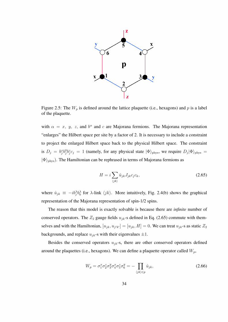
Figure 2.5: The Wp is defined around the lattice plaquette (i.e., hexagons) and p is a labelof the plaquette.

with α = x, y, z, and bα and c are Majorana fermions. The Majorana representation

“enlarges” the Hilbert space per site by a factor of 2. It is necessary to include a constraint

to project the enlarged Hilbert space back to the physical Hilbert space. The constraint

is Dj = bxj byj bzjcj = 1 (namely, for any physical state |Φ〉phys, we require Dj|Φ〉phys =

|Φ〉phys). The Hamiltonian can be rephrased in terms of Majorana fermions as

H = i∑〈jk〉

ujkJjkcjck, (2.65)

where ujk ≡ −ibλj bλk for λ-link 〈jk〉. More intuitively, Fig. 2.4(b) shows the graphical

representation of the Majorana representation of spin-1/2 spins.

The reason that this model is exactly solvable is because there are infinite number of

conserved operators. The Z2 gauge fields ujk-s defined in Eq. (2.65) commute with them-

selves and with the Hamiltonian, [ujk, uj′k′ ] = [ujk, H] = 0. We can treat ujk-s as static Z2

backgrounds, and replace ujk-s with their eigenvalues ±1.

Besides the conserved operators ujk-s, there are other conserved operators defined

around the plaquettes (i.e., hexagons). We can define a plaquette operator called Wp,

Wp = σx1σz2σ

y3σ

x4σ

z5σ

y6 = −

∏〈jk〉∈p

ujk, (2.66)

34

around a lattice plaquette p, Fig. 2.5. Since ujk-s commute with themselves and with the

Hamiltonian, so are the Wp plaquette terms. Each Wp term also has eigenvalues ±1.

Around each plaquette p, one can define the “fluxes” φp via e−iφp ≡∏〈jk〉∈p iujk. The

most interesting choice of ujk is the one that minimizes the ground state energy. The answer

is provided by Lieb [62] saying that the ground state is the “uniform-flux” state. Therefore,

we can simply assume that ujk = 1 for all link 〈jk〉, where j belongs to even sublattice,

and k belongs to the odd sublattice.

In order to diagonalize the Majorana Hamiltonian, first we note that because a Majo-

rana Fermion is its own antiparticle, there is always the “particle-hole” symmetry in any

general Majorana Hamiltonian. Due to such symmetry, only half of the degrees of freedom

in the Majorana Hamiltonian are physical. For instance, for an eigenvector-eigenenergy

pair, {~vk, εk}, there is a corresponding pair, {~vk′ , εk′} = {~v∗−k′ ,−ε−k} that is related by

the particle-hole symmetry. More mathematically, we can introduce the expansion of the

original Majoranas in terms of usual complex fermions as

c(r, a) =

√2

Nuc

∑εk>0,k∈B.Z.

[eik·rvk(a)f(k) + H.c.

], (2.67)

where for clarity, we introduce j = (r, a) with r running over the Bravais lattice of unit

cells, a = 1, 2 the sublattice labeling in a unit cell. Nuc is the number of unit cells, and the

complex Fermion f satisfies the usual anticommutation relation. The canonical form of the

Hamiltonian is

H =∑

εk>0,k∈B.Z.

2εk

[f †(k)f(k)− 1

2

]. (2.68)

In the present model on the honeycomb lattice, εk = |Jxeik·n1 + Jyeik·n2 + Jz|, with

n1/2 = (±1/2,√

3/2) in the standard xy-coordinates. An important property of the

spectrum is whether it is gapless, i.e., whether εk is zero for some k. The equation

Jxeik·n1 + Jye

ik·n2 + Jz = 0 has a solution if and only if Jx, Jy, and Jz (we assume

35

Az

Ax Ay

B

Jz = 1, Jx=Jy=0

Jx = 1,

Jy=Jz=0

Jy = 1,

Jx=Jz=0

gapless

gapped

(a) (b)

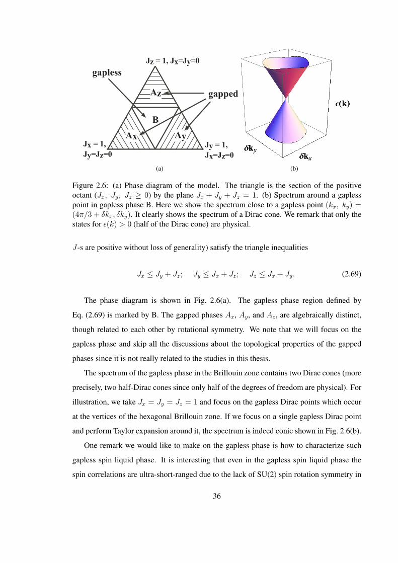
Figure 2.6: (a) Phase diagram of the model. The triangle is the section of the positiveoctant (Jx, Jy, Jz ≥ 0) by the plane Jx + Jy + Jz = 1. (b) Spectrum around a gaplesspoint in gapless phase B. Here we show the spectrum close to a gapless point (kx, ky) =(4π/3 + δkx, δky). It clearly shows the spectrum of a Dirac cone. We remark that only thestates for ε(k) > 0 (half of the Dirac cone) are physical.

J-s are positive without loss of generality) satisfy the triangle inequalities

Jx ≤ Jy + Jz; Jy ≤ Jx + Jz; Jz ≤ Jx + Jy. (2.69)

The phase diagram is shown in Fig. 2.6(a). The gapless phase region defined by

Eq. (2.69) is marked by B. The gapped phases Ax, Ay, and Az, are algebraically distinct,

though related to each other by rotational symmetry. We note that we will focus on the

gapless phase and skip all the discussions about the topological properties of the gapped

phases since it is not really related to the studies in this thesis.

The spectrum of the gapless phase in the Brillouin zone contains two Dirac cones (more

precisely, two half-Dirac cones since only half of the degrees of freedom are physical). For

illustration, we take Jx = Jy = Jz = 1 and focus on the gapless Dirac points which occur

at the vertices of the hexagonal Brillouin zone. If we focus on a single gapless Dirac point

and perform Taylor expansion around it, the spectrum is indeed conic shown in Fig. 2.6(b).

One remark we would like to make on the gapless phase is how to characterize such

gapless spin liquid phase. It is interesting that even in the gapless spin liquid phase the

spin correlations are ultra-short-ranged due to the lack of SU(2) spin rotation symmetry in

36

this model. In order to give a gauge-invariant characterization of such Kitaev-type gapless

spin liquids, we suggest that the gaplessness can be detected by the local bond-energy

correlations. The approach is detailed in our paper [63], which we do not include in this

thesis because we will focus on SU(2)-invariant spin liquids in the remaining chapters.

Finally, the Kitaev model on the honeycomb lattice has many impacts on several fields

including not only the new ways to study spin liquids, but also sheding light on the topolog-

ical quantum computations. It is impossible to cover all the topics about the Kitaev model.

For readers that are interested in all the details, please consult [14].

37

Chapter 3

Two-band electronic metal andneighboring spin liquid (spinBose-metal) on a zigzag strip withlonger-ranged repulsion

We mentioned in Chapter 2.3.1 that SBM phase can be accessed by bosonizing interacting

electrons system. In this chapter, we focus on realizing such scenario for the SBM in

explicit and realistic electronic models. Specifically, we start in the metallic phase with

two gapless charge modes and two gapless spin modes—so-called “C2S2” metal. We can

imagine gapping out just the overall charge mode to obtain a “C1S2” Mott insulator with

one gapless “charge” mode and two gapless spin modes, where the former represents local

current loop fluctuations and does not transport charge along the chain. This is precisely

the SBM phase. If one thinks of a spin-only description of this Mott insulator, the gapless

“charge” mode can be interpreted as spin singlet chirality mode.

Recently, Hubbard model on the zigzag chain (t1 − t2 − U chain) has received much

attention [64, 65, 66, 67, 68, 69]. For free electrons, the two-band metal appears for t2/t1 >

0.5. However, in the case of Hubbard interaction, weak coupling approach [65, 66] finds

that this phase is stable only over a narrow range t2/t1 ∈ [0.5, 0.57], while a spin gap opens

up for larger t2/t1. The Umklapp that can drive a transition to a Mott insulator requires

eight fermions and is strongly irrelevant at weak coupling. Prior work [49, 64, 65] focused

on the spin-gapped metal and eventual spin-gapped insulator for strong interaction, while

the C1S2 spin liquid phase was not anticipated.

38

There have also been numerical DMRG studies of the Hubbard model [67, 68, 69,

66]. The focus has been on the prominent spin-gapped phases and, in particular, on the

insulator that is continuously connected to the dimerized phase in the J1 − J2 Heisenberg

model, which is appropriate in the strong interaction limit U � t1, t2. The C2S2 metallic

phase and possibility of nearby spin liquid on the Mott insulator side in the Hubbard model

have not been explored. We hope our work will motivate more studies of this interesting

possibility in the Hubbard model with intermediate U close to the C2S2 metal.

Since the C2S2 metallic phase is quite narrow in the Hubbard model, we would like to

first widen the C2S2 region. To this end, we explore an electronic model with extended

repulsive interactions. [70] Such interactions tend to suppress instabilities in the electronic

system, similar to how long-ranged Coulomb repulsion suppresses pairing in metals. They

are also more realistic than the on-site Hubbard, particularly for materials undergoing a

metal-insulator transition where there is no conduction band screening on the insulator

side. Thus, recent ab initio model construction for the κ-(ET)2Cu2(CN)3 material found

significant extended interactions in the corresponding electronic model on the half-filled

triangular lattice [39, 38].

Applying weak coupling renormalization group (RG) approach to the zigzag ladder sys-

tem [49, 64, 71, 65], we indeed find that extended interactions open a much wider window

of the C2S2 metal phase. Building on this, we then use bosonization approach to explore

a transition to a Mott insulator upon increasing the overall repulsion strength. We find that

such longer-ranged interactions can drive the system into the C1S2 spin liquid Mott insu-

lator rather than a spin-gapped insulator. This bodes well for finding spin liquid phases in

more realistic electronic models for materials near the metal-insulator transition.

This chapter is organized as follows. In Chapter 3.1, we set up the weak coupling RG

[49, 71, 65] and open a much wider window of the metallic C2S2 phase by introducing real-

istically motivated longer-ranged repulsion. In Chapter 3.2, we use bosonization to extend

the analysis to intermediate coupling. We gradually increase the overall repulsion strength

and determine thresholds for a Mott transition driven by the eight-fermion Umklapp term

and also for spin gap instabilities, thus mapping out phases neighboring the C2S2 metal. In

Chapter 3.3, we summarize our results and conclude with some discussion.

39

3.1 Weak coupling analysis of t1− t2 model with extended

repulsion: Stabilizing C2S2 metal

3.1.1 Setup for two-band electron system

We consider half-filled electronic t1 − t2 model with extended interaction described by the

Hamiltonian H = H0 +HV , with

H0 = −∑x,α

[t1c†α(x)cα(x+ 1) + t2c

†α(x)cα(x+ 2) + H.c.

],

HV =1

2

∑x,x′

V (x− x′)n(x)n(x′) . (3.1)

Here c(c†) is fermion annihilation (creation) operator, x is a site label on the one-dimensional

(1D) chain, and α =↑, ↓ is a spin index; n(x) ≡∑

α c†α(x)cα(x) is electron number on the

site.

In weak coupling, the kinetic energy Eq. (3.1) gives free particle dispersion

ε(k) = −2t1 cos(k)− 2t2 cos(2k) . (3.2)

For t2/t1 > 0.5, there are two sets of Fermi points at wavevectors ±kF1 and ±kF2 as

shown in Fig. 3.1. We adopt the same conventions as in [29]. Fermions near kF1 and kF2

are moving to the right, and the corresponding group velocities are v1, v2 > 0. Electrons

are at half-filling, which implies kF1+kF2 = −π/2 mod 2π for the choices, as in Fig. 3.1.

The electron operators are expanded in terms of continuum fields,

cα(x) =∑P,a

eiPkFaxcPaα , (3.3)

with P = R/L = +/− denoting the right and left movers and a = 1, 2 denoting the two

Fermi seas.

Four-fermion interactions can be conveniently expressed in terms of chiral currents

40

-5

-4

-3

-2

-1

0

1

2

3

-π 0 πε(k

)k

kF1-kF1kF2 -kF2

kF2 = -kF1 - π/2

-2 t1 cos(k) - 2 t2 cos(2k) - µ

Figure 3.1: The electron band for t2 > 0.5t1 has two occupied Fermi sea segments. This isfree fermion C2S2 metal.

[49, 71, 29],

JPab =∑α

c†PaαcPbα , (3.4)

~JPab =∑α,β

c†Paα~σαβ2cPbβ . (3.5)

Most general four-fermion interactions can be written as

HρRL =

∑a,b

(wρabJRabJLab + λρabJRaaJLbb

), (3.6)

HσRL = −

∑a,b

(wσab

~JRab · ~JLab + λσab~JRaa · ~JLbb

), (3.7)

Hρchiral =

1

2

∑a

Cρaa

(JRaaJRaa + JLaaJLaa

)+Cρ

12

(JR11JR22 + JL11JL22

), (3.8)

Hσchiral = −1

2

∑a

Cσaa

(~JRaa · ~JRaa + ~JLaa · ~JLaa

)−Cσ

12

(~JR11 · ~JR22 + ~JL11 · ~JL22

). (3.9)

Here HRL are terms that connect right and left movers, while Hchiral are chiral terms with

all fermions moving in the same direction.

Consider the couplings in HRL. We have w11 = w22 = 0 (convention), w12 = w21

(from hermiticity), and λ12 = λ21 (from R ↔ L symmetry). Thus there are 8 independent

41

couplings: wρ/σ12 , λρ/σ11 , λ

ρ/σ22 , and λρ/σ12 . Note that there are no four-fermion Umklapp terms

in our two-band system.

In the specific lattice model, we expand the interactions Eq. (3.1) in terms of the con-

tinuum fields and find “bare” values of the couplings:

λρ11 = VQ=0 −V2kF1

2, (3.10)

λρ22 = VQ=0 −V2kF2

2, (3.11)

λρ12 = VQ=0 −Vπ/2

2, (3.12)

λσ11 = 2V2kF1, (3.13)

λσ22 = 2V2kF2, (3.14)

λσ12 = 2Vπ/2 , (3.15)

wρ12 = VkF1−kF2−Vπ/2

2, (3.16)

wσ12 = 2Vπ/2 , (3.17)

Cρ11 = Cρ

22 = VQ=0 −U

2, (3.18)

Cρ12 = VQ=0 −

VkF1−kF2

2, (3.19)

Cσ11 = Cσ

22 = 2U , (3.20)

Cσ12 = 2VkF1−kF2

. (3.21)

Here VQ ≡∑∞

x′=−∞ V (x − x′)eiQ(x−x′) = V−Q, since V (x − x′) = V (x′ − x). We have

also used explicitly kF1 + kF2 = −π/2.

The termsHchiral renormalize “velocities” of various modes. In the weak-coupling RG

analysis, they only generate higher-order contributions and are therefore not important.

The RG equations below contain only couplings from HRL. On the other hand, the chiral

interactions are important in the intermediate coupling analysis to be done in Chapter 3.2,

which is why we have listed their values as well. The on-site coupling U ≡ V (x− x′ = 0)

appears explicitly in Cρ/σ11 and Cρ/σ

22 because of our more careful treatment of the on-site

interaction, which we first write as Un↑(x)n↓(x) and then insert the continuum fields (and

bosonize in Chapter 3.2).

42

3.1.2 Weak coupling renormalization group

The RG equations in the two-band system are [49, 71, 65]:

λρ11 = − 1

2πv2

[(wρ12)2 +

3

16(wσ12)2

], (3.22)

λρ22 = − 1

2πv1

[(wρ12)2 +

3

16(wσ12)2

], (3.23)

λρ12 =1

π(v1 + v2)

[(wρ12)2 +

3

16(wσ12)2

], (3.24)

λσ11 = − 1

2πv1

(λσ11)2 − 1

4πv2

[(wσ12)2 + 4wρ12w

σ12

], (3.25)

λσ22 = − 1

2πv2

(λσ22)2 − 1

4πv1

[(wσ12)2 + 4wρ12w

σ12

], (3.26)

λσ12 = − 1

π(v1 + v2)

{(λσ12)2 +

(wσ12)2 − 4wρ12wσ12

2

}, (3.27)

wρ12 = −Λρwρ12 −3

16Λσwσ12 , (3.28)

wσ12 = −Λσwρ12 −(

Λρ +Λσ

2+

2λσ12

π(v1 + v2)

)wσ12 . (3.29)

Here O ≡ ∂O/∂`, where ` is logarithm of the length scale. We have also defined

Λρ/σ =λρ/σ11

2πv1

+λρ/σ22

2πv2

− 2λρ/σ12

π(v1 + v2). (3.30)

Details of our system enter through the band velocities v1, v2, and the initial conditions

Eqs. (3.10)–(3.17).

3.1.3 Fixed point for stable C2S2 phase

We are primarily interested in the stability of the two-band metallic phase with two gapless

charge and two gapless spin modes —“C2S2” in the notation of [49]. In the RG, this phase

is characterized as having no divergent couplings. Before proceeding with detailed numer-

ical studies of the flow Eqs. (3.22)–(3.29), we can describe such stable C2S2 fixed point

qualitatively: The charge sector couplings reach some fixed values, λρ∗11, λρ∗22, λ

ρ∗12, and are

strictly marginal; they also need to satisfy Λρ∗ > 0 (see below). The spin sector couplings

43

approach zero from positive values, λσ∗11 = λσ∗22 = λσ∗12 = 0+, and are marginally irrelevant.

Finally, the “charge-spin” couplings w12 go to zero, wρ∗12 = wσ∗12 = 0, and are irrelevant,

which is insured by the condition Λρ∗ > 0. Indeed, consider small deviations of compa-

rable magnitudes for all couplings and allowing only positive λσab. Since we have finite

Λρ∗ > 0, first the wρ/σ12 will renormalize quickly to zero, without significantly affecting the

other couplings. Then the λσab will renormalize to zero via slow marginal flows.

3.1.4 Numerical studies of the flows

We can solve the RG equations numerically for given initial conditions and check whether

the couplings flow into the domain of attraction of the C2S2 fixed point or not. We use

Mathematica to solve the flows up to long “time” ` when the ultimate trends become ap-

parent.

If the couplings always remain of the same order as their initial values or approach zero,

we say the couplings are marginal or irrelevant and identify this as the C2S2 phase. The

eventual trends here were discussed in Chapter 3.1.3.

On the other hand, if the magnitudes of some couplings grow significantly compared to

the initial values, we say that the couplings are relevant and the C2S2 phase is destroyed.

Thus, if either λσ11 or λσ22 coupling becomes negative while wσ12 and wρ12 remain of the same

sign, this λσ then runs away to large negative values and also induces the other couplings

to diverge. Bosonizing the four-fermion interactions [49, 71, 29] (see Chapter 3.2), we

can see that two spin modes and one charge mode become gapped and we obtain so-called

“C1S0” phase. The overall charge propagation mode remains gapless and the system is

conducting. Note that we do not distinguish which coupling diverges faster in the formal

flow Eqs. (3.22)–(3.29). As discussed in [49], in the U → 0+ limit one can separate a

so-called “C2S1” case where one of the spin couplings diverges qualitatively faster (but all

couplings still diverge at the same `). We do not make such subtle distinction and call any

runaway flow situation as C1S0—all we want to know is that the two-band metal C2S2

became unstable.

The RG flows are qualitatively similar for different points in the same phase, so we only

44

ΛabΡ

ΛabΣ

w12Ρ

w12Σ

-12

-10

-8

-6

-4

Log@CouplingD

l

Figure 3.2: (Color online) Example of RG flows in the C2S2 phase. The model potential isEq. (3.31) with κ = 1/2, γ = 2/5; the band parameter is t2/t1 = 0.9. We choose logarithmof the couplings to be the y-axis and RG “time” ` to be the x-axis. We see that wρ/σ12 flowstoward 0 rapidly (irrelevant couplings); λρab saturates very fast (strictly marginal couplings);while λσab flows to 0 slowly (marginally irrelevant). More generally, if we fix these κ and γvalues, for t2/t1 < 0.99 the flows are similar to those shown here, and the phase is C2S2.

show one representative picture for each case. Fig. 3.2 shows the flows in the C2S2 phase.

The scale parameter ` is the x-axis, while logarithm of the couplings is the y-axis. In this

way, we clearly see that the couplings separate into three groups, which is well explained

by the C2S2 fixed point in Chapter 3.1.3: the wρ/σ12 flow to 0 exponentially rapidly, the λσab

flow to 0 marginally slowly, while the λρab saturate.

Fig. 3.3 illustrates the flows in the C1S0 phase. Here we use real values of the coupling

as the y-axis and only show selected couplings, λσ11, λσ22, wρ12, and wσ12. We clearly see that

these couplings diverge (and so do the other couplings not shown in the figure).

3.1.5 Examples of phase diagrams with C2S2 metal stabilized by ex-

tended interactions

For illustration in our chapter, we consider the following interaction potential,

V (x− x′) =

U , |x− x′| = 0

κUe−γ|x−x′| , |x− x′| ≥ 1

. (3.31)

Here U is the overall energy scale and also the on-site repulsion. The relative magnitude

of the extended repulsion is set by some factor κ < 1. Beyond one lattice spacing, the

45

w12

Ρ

w12Σ

Λ11Σ Λ22

Σ

0.010

0.005

0.005

0.010

Coupling

l

Figure 3.3: (Color) Example of RG flows of selected couplings in the C1S0 phase. Themodel is the same as in Fig. 3.2, but with t2/t1 = 1.05. We see that the selected couplingsdiverge after some time. For example, once the λσ11 and λσ22 become negative while wρ12

and wσ12 remain positive, the RG equations (3.22)–(3.29) drive the λσ11 and λσ22 to -∞ and inturn wρ12 and wσ12 to +∞, and then all couplings diverge. More generally, if we fix γ = 2/5,for t2/t1 > 0.99 the flows are similar to those shown here and we call this the C1S0 phase.Varying γ, we obtain the phase diagram Fig. 3.4.

potential decreases exponentially with decay rate γ. For γ → ∞ we obtain the Hubbard

model with on-site interaction only, while for small γ the interaction extends over many

lattice sites.

We also consider the above potential but truncated at the 4th neighbor. This tests ro-

bustness of our conclusions to modifications where the interactions have finite but still

somewhat extended range, as may be preferable in numerical studies of such electronic

models.

3.1.5.1 Weak coupling phase diagram for potential Eq. (3.31)

The extended repulsion, Eq. (3.31), is in Fourier space

VQ = U

[1− κ+

κ sinh(γ)

cosh(γ)− cos(Q)

]. (3.32)

For given model parameters, we use Eqs. (3.10)–(3.17) to set initial conditions. We follow

the RG flows and identify the phases as described above, thus mapping out the “weak

coupling phase diagram”. Here and in the rest of the chapter, we take κ = 0.5. This is

loosely motivated by the recent ab initio calculation [39] for the κ-(ET)2Cu2(CN)3, which

46

0.6 0.8 1 1.2 1.4 1.60

0.2

0.4

0.6

0.8

1

1.2

1.4

1.6

1.8

C2S2 Boundary!

t2/t1

C2S2

0.57

C1S0

0.5

Figure 3.4: Stabilization of the C2S2 metal by extended interactions. The model potentialis Eq. (3.31) with κ = 0.5. The noninteracting problem has one band for t2/t1 < 0.5and two bands for t2/t1 > 0.5, see Fig. 3.1, and we focus on the latter region. The limitγ → ∞ corresponds to the Hubbard model with on-site repulsion only, and the C2S2phase is stable only over a narrow window t2/t1 ∈ [0.5 . . . 0.57] [65, 49]. The C2S2 regionbecomes progressively wider as we increase the interaction range 1/γ.

gives the ratio of the nearest-neighbor repulsion V1 ≡ V (|x − x′| = 1) to the on-site

Hubbard U as V1/U ' 0.43, while in our model V1/U = κe−γ . The corresponding phase

diagram showing stable C2S2 region is in Fig. 3.4.

We see that the C2S2 region becomes wider upon increasing the interaction range 1/γ.

We can understand this qualitatively as follows. For fixed band parameters, when γ → 0

the values of VQ for all nonzero Q approach U(1− κ), while VQ=0 ' 2κU/γ continues to

increase. The corresponding contribution to Λρ is

δΛρ =VQ=0

2π

[1

v1

+1

v2

− 4

v1 + v2

]=VQ=0

2π

[(v1 − v2)2

v1v2(v1 + v2)

], (3.33)

which is positive for any v1 6= v2 and grows with increasing VQ=0. Note also from

Eqs. (3.10)–(3.17) that the VQ=0 enters only in the λρab couplings. Large bare value of

Λρ makes the wρ/σ12 flows strongly irrelevant. Their effect on the λσab flows is rapidly de-

creasing and expires. The λσab couplings start repulsive and stay so and eventually flow to

zero via marginal flows. This argument is strictly true in the small γ limit, while for finite

γ the interplay of different flows is more complex and requires numerical study, as done in

Fig. 3.4.

47

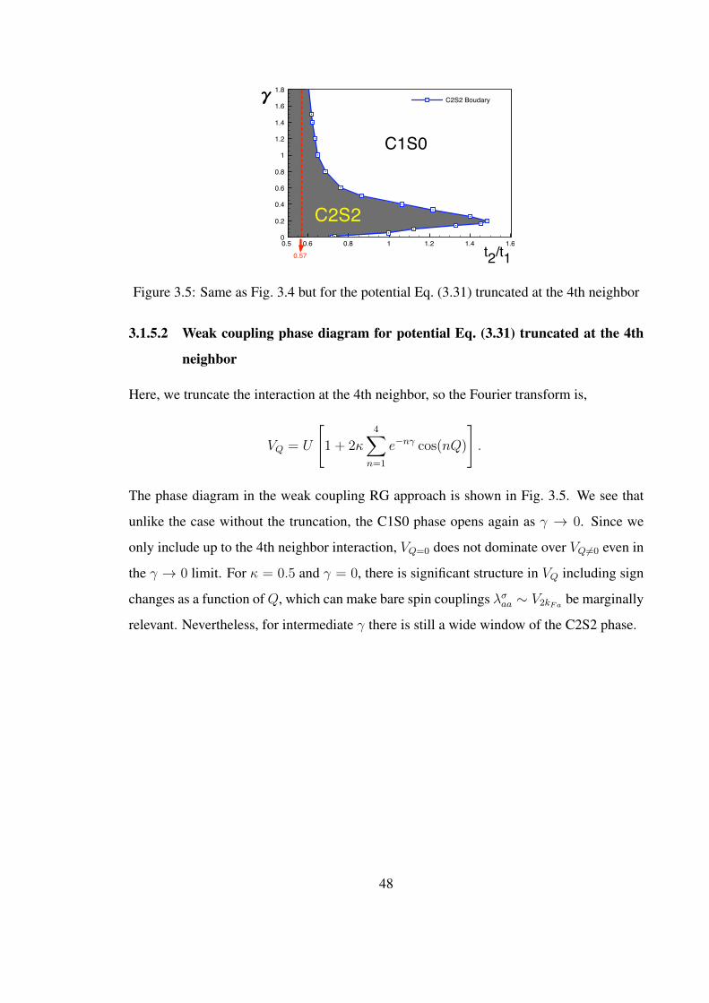
0.6 0.8 1 1.2 1.4 1.60

0.2

0.4

0.6

0.8

1

1.2

1.4

1.6

1.8

C2S2 Boudary

t2/t1

!

C2S2

0.57

C1S0

0.5

Figure 3.5: Same as Fig. 3.4 but for the potential Eq. (3.31) truncated at the 4th neighbor

3.1.5.2 Weak coupling phase diagram for potential Eq. (3.31) truncated at the 4th

neighbor

Here, we truncate the interaction at the 4th neighbor, so the Fourier transform is,

VQ = U

[1 + 2κ

4∑n=1

e−nγ cos(nQ)

].

The phase diagram in the weak coupling RG approach is shown in Fig. 3.5. We see that

unlike the case without the truncation, the C1S0 phase opens again as γ → 0. Since we

only include up to the 4th neighbor interaction, VQ=0 does not dominate over VQ 6=0 even in

the γ → 0 limit. For κ = 0.5 and γ = 0, there is significant structure in VQ including sign

changes as a function ofQ, which can make bare spin couplings λσaa ∼ V2kFa be marginally

relevant. Nevertheless, for intermediate γ there is still a wide window of the C2S2 phase.

48

3.2 Weak-to-intermediate coupling: Phases out of C2S2

upon increasing interaction

3.2.1 Harmonic description of the C2S2 phase

Let us begin with a harmonic description of the C2S2 metal. Technical steps and many

details of the bosonization essentially follow [29] and references therein. We write

cPaα = ηaαei(ϕaα+Pθaα) , (3.34)

where ϕ and θ are canonically conjugate boson fields and η are Klein factors.

We define “charge” and “spin” boson fields,

θaρ/σ =1√2

(θa↑ ± θa↓) , (3.35)

and “even” and “odd” flavor combinations,

θµ± =1√2

(θ1µ ± θ2µ) , (3.36)

with µ = ρ, σ. Similar definitions hold for the ϕ fields.

We can now bosonize all four-fermion interactions Eqs. (3.6)–(3.9). First consider the

spin sector. The Cσab terms give velocity renormalizations, while the λσab terms are written

out in Sec. IVA of [29] and are not repeated here. We assume that the λσab are marginally

irrelevant in the C2S2 phase. The fixed-point Lagrangian has effectively decoupled boson

fields θ1σ and θ2σ with Luttinger parameters g1σ = g2σ = 1, dictated by SU(2) spin rotation

invariance.

The Lagrangian in the charge sector is

Lρ =1

2π

[∂xΘ

T ·A · ∂xΘ + ∂xΦT ·B · ∂xΦ

]+i

π∂xΘ

T · ∂τΦ , (3.37)

49

where we defined ΘT = (θρ+, θρ−) and ΦT = (ϕρ+, ϕρ−). Matrix elements of A and B

are:

A11 = v +λρ11 + λρ22 + 2λρ12

2π+Cρ

11 + Cρ22 + 2Cρ

12

2π

= v +4VQ=0

π− V2kF1

4π− V2kF2

4π−Vπ/22π− VkF1−kF2

2π− U

2π, (3.38)

A22 = v +λρ11 + λρ22 − 2λρ12

2π+Cρ

11 + Cρ22 − 2Cρ

12

2π

= v − V2kF1

4π− V2kF2

4π+Vπ/22π

+VkF1−kF2

2π− U

2π, (3.39)

A12 = A21 = vr +λρ11 − λ

ρ22

2π+Cρ

11 − Cρ22

2π= vr −

V2kF1

4π+V2kF2

4π, (3.40)

B11 = v − λρ11 + λρ22 + 2λρ12

2π+Cρ

11 + Cρ22 + 2Cρ

12

2π

= v +V2kF1

4π+V2kF2

4π+Vπ/22π− VkF1−kF2

2π− U

2π, (3.41)

B22 = v − λρ11 + λρ22 − 2λρ12

2π+Cρ

11 + Cρ22 − 2Cρ

12

2π

= v +V2kF1

4π+V2kF2

4π−Vπ/22π

+VkF1−kF2

2π− U

2π, (3.42)

B12 = B21 = vr −λρ11 − λ

ρ22

2π+Cρ

11 − Cρ22

2π= vr +

V2kF1

4π− V2kF2

4π, (3.43)

where

v ≡ v1 + v2

2, vr ≡

v1 − v2

2. (3.44)

The couplings λρab of the right–left mixing interactions HρRL enter with opposite signs in

A and B and directly affect Luttinger parameters, while the couplings Cρab of Hρ

chiral enter

with the same sign and give velocity renormalizations.

From the final expressions in terms of VQ, we see that the Q = 0 component enters

only in A11. This can be understood by considering the Q = 0 part of the interaction, [70]

∑x,x′

V (x− x′)n(x)n(x′) → VQ=0

∫x

[ρ(x)]2 (3.45)

where ρ(x) = 2∂xθρ+/π is the coarse-grained electron density.

50

Note also that the −U/(2π) in the diagonal matrix elements is due to our more careful

treatment of the on-site repulsion, which we first write as Un↑(x)n↓(x) and then bosonize.

We obtain harmonic description of the C2S2 phase by combining the spin and charge

sectors. The latter two-mode system Lρ has nontrivial Luttinger parameters, which can

be determined from the matrices A and B (see Appendix 3.A). The fixed-point matrix

elements will differ somewhat from the bare values above, but we ignore this in our crude

analysis of the intermediate coupling regime.

To complete the bosonization of the four-fermion interactions, Eqs. (3.6)–(3.9), the

wρ/σ12 terms give [71, 29]

W ≡(wρ12JR12JL12 − wσ12

~JR12 · ~JL12

)+ H.c. (3.46)

= cos(2ϕρ−)

{4wρ12

[cos(2ϕσ−)− Γ cos(2θσ−)

]−wσ12

[cos(2ϕσ−) + Γ cos(2θσ−) + 2Γ cos(2θσ+)

]}, (3.47)

where Γ = η1↑η1↓η2↑η2↓. We see that W couples the charge and spin sectors. In the C2S2

theory described above, its scaling dimension is,

∆[W ] = ∆[cos(2ϕρ−)] + 1 , (3.48)

where ∆[cos(2ϕρ−)] is evaluated in the Lagrangian Lρ, while the contribution 1 comes

from the spin sector. For the C2S2 theory to be consistent, the W term must be irrelevant,

∆[W ] > 2. Once the W renormalizes to zero, the charge and spin sectors decouple.

We thus have precise parallel with the weak coupling analysis of the C2S2 fixed point in

Chapter 3.1.

On the other hand, if ∆[W ] < 2, the W term becomes relevant and the C2S2 state is

unstable. In this case, ϕρ− will get pinned and also the spin sector will become gapped.

Only the “ρ+” mode remains gapless and the system is some C1S0 conducting phase.

51

3.2.2 Mott insulator driven by Umklapp interaction. Intermediate

coupling procedure out of the C2S2

The weak coupling analysis in Chapter 3.1 misses the possibility of gapping out the overall

charge mode θρ+ since there are no four-fermion Umklapp terms allowed in the two-band

system. However, the half-filled electronic system does become a Mott insulator for suffi-

ciently strong repulsion. In the theoretical description, this is achieved by an eight-fermion

Umklapp term [29]

H8 = v8(c†R1↑c†R1↓c

†R2↑c

†R2↓cL1↑cL1↓cL2↑cL2↓ + H.c.)

= 2v8 cos(4θρ+) . (3.49)

At weak coupling, this term has scaling dimension ∆[H8] = 4 and is strongly irrelevant.

However, from Eq. (3.45) we see that overall repulsive interaction stiffens the θρ+ mode and

lowers the scaling dimension of H8. For sufficiently strong repulsion, ∆[H8] drops below

2 and the Umklapp becomes relevant; θρ+ gets pinned and we obtain a Mott insulator.

Our intermediate coupling procedure is as follows. Using the harmonic theory of

the C2S2 phase, we calculate the scaling dimensions ∆[W ], Eq. (3.48), and ∆[H8] =

∆[cos(4θρ+)] from the Lagrangian Lρ, Eq. (3.37). Details are described in Appendix 3.A

and calculations are done numerically in the end.

If both ∆[W ] and ∆[H8] are larger than 2, the C2S2 metal is stable. As interactions

increase, eventually either W or H8 becomes relevant. In general, there are two cases:

1) If H8 becomes relevant first, we pin θρ+ and enter “C1S2” Mott insulator. To be

more precise, we can further qualify the label as “C1[ρ−]S2”; the remaining “charge”

mode “ρ−” represents local current loop fluctuations and does not conduct. This is the

spin liquid phase called spin Bose-metal in [29] and described in detail there. Exploring

conditions for finding such phase in electronic models is our main goal here.

2) On the other hand, if the W term becomes relevant first, we enter C1S0 conducting

state with a spin gap (more precisely, “C1[ρ+]S0”).

Some reservations are in order. First, we use bare values of the couplings in the A

52

and B matrices, which is not accurate since the couplings experience initial flows, see

Chapter 3.1.2. Second, we consider only instabilities driven by changes in the harmonic Lρ

theory as they translate to scaling dimensions of the H8 and W terms, i.e., we effectively

treat the latter as small. We also assume that the spin sector is near the fixed point with

all λσab marginally irrelevant and small. We will address these reservations after presenting

results of the above procedure. Keeping these remarks in mind, we now describe how we

analyze phases out of the C1[ρ−]S2 and C1[ρ+]S0 in the same procedure.

3.2.2.1 Instability out of C1[ρ−]S2 driven by spin-charge coupling W

In the present analysis focusing on the “ρ+” and “ρ−” fields, we can also crudely estimate

the extent of the C1S2 or C1S0 phases once either happens out of the C2S2.

Suppose the UmklappH8 is relevant first and we are in the C1S2 phase. We still need to

remember theW term since it can become relevant if we continue increasing the interaction

strength. To estimate the scaling dimension of the W term, we assume now that the θρ+

field is massive and integrate out θρ+ and ϕρ+. Mathematically this amounts to sending

A11 →∞, and we obtain

∆ [W ; θρ+ is pinned] =

[A22B11

B11B22 −B212

] 12

+ 1 . (3.50)

This assumption is approximate but reasonable, since once the parameters are such that

the system is in the C1S2 phase, the relevant H8 will grow and quickly stiffen the A11 in

positive feedback loop.

The C1S2 phase is stable if ∆[W ] > 2, and this analysis is similar to the stability

analysis of the SBM in [29]. If ∆[W ] drops below 2, the W term becomes relevant and

the ϕρ− field will be pinned, together with gapping out the spin sector, see Eq. (3.47). The

final result is some “C0S0” phase, whose precise character depends on the details of the

couplings wρ/σ12 . This is studied in Sec. IVB of [29]. For the present repulsive electron

model, we have wρ12, wσ12 > 0, so the resulting C0S0 is likely a period-2 valence bond solid

(VBS). [29] This connects to dimerized phase in the J1 − J2 spin chain appropriate in the

strong interaction limit of the electron system.

53

3.2.2.2 Instability out of C1[ρ+]S0 driven by Umklapp H8

Suppose now the W interaction becomes relevant first. From Eq. (3.47), it is natural that

ϕρ− is pinned, the spin sector gets gapped, and we are in C1S0 phase. Here we postulate

mass for ϕρ− (essentially sending B22 →∞) and calculate the effective scaling dimension

of the Umklapp term,

∆ [H8; ϕρ− is pinned] = 4

[B11A22

A11A22 − A212

] 12

. (3.51)

If ∆[H8] > 2, the C1S0 is stable. Once ∆[H8] drops below 2, the overall charge mode

θρ+ is pinned and we obtain fully gapped Mott insulator C0S0, which is likely the same

period-2 VBS discussed earlier.

3.2.3 Numerical results

We consider the same models with extended density-density interactions as in the weak

coupling analysis in Chapter 3.1.5, parking ourselves initially in the C2S2 phase in Fig. 3.4

and Fig. 3.5. From the preceding discussion, we can obtain two phases out of the C2S2

upon increasing interaction strength—either C1[ρ+]S0 or C1[ρ−]S2. To visualize the re-

sults, we imagine adding the overall interaction strength V as the z-axis to Fig. 3.4 and

Fig. 3.5. We then project down which phase happens first for each such vertical line out of

C2S2. Calculations are done numerically and the results are shown in Fig. 3.6 and Fig. 3.9.

In Fig. 3.7 we take a cut through Fig. 3.6 at γ = 0.4 and show details of the phase diagram

in the t2/t1 − V plane.

3.2.3.1 Intermediate coupling phase diagram for model with potential Eq. (3.31)

Fig. 3.6 shows results for the model potential Eq. (3.31). We can see that in two regimes

γ ≥ 1.2 and γ ≤ 0.4 we exit from the C2S2 into the C1S2. The two limits can be

understood analytically.

In the large γ case, we can replace all VQ by simply U . The matrices A and B defined

54

0.6 0.8 1 1.2 1.4 1.60

0.2

0.4

0.6

0.8

1

1.2

1.4

1.6

1.8

!

t2/t1

C2S2 C1S2(SBM)

C2S2 C1S0

0.5

Figure 3.6: Projection of phases obtained out of the C2S2 of Fig. 3.4 as we increase overallrepulsion strength V , which we imagine to be the z-axis perpendicular to the page (Fig. 3.7gives one cut at γ = 0.4 with such V axis shown explicitly). The results are obtained inthe intermediate coupling procedure as explained in the text. White region is C1S0 at weakcoupling, see Fig. 3.4, and is not considered here.

in Eq. (3.38)–(3.43) become

A =

v + 2Uπ

vr

vr v

, B =

v vr

vr v

. (3.52)

We see that U only contributes to A11. This monotonically “stiffens” the θρ+ (lowering

∆[H8]) but “softens” the ϕρ− (increasing ∆[W ]). Therefore we only expect the C1S2

phase out of the C2S2 as found in the numerical calculations.

On the other hand, for small γ we can see from Eq. (3.32) that VQ=0 will dominate over

VQ 6=0. Keeping only VQ=0, the matrices A and B become

A '

v +4VQ=0

πvr

vr v

, B '

v vr

vr v

. (3.53)

Thus the small γ case has similar mathematical structure to the large γ case. The physical

difference is that here the transition to the C1S2 is driven by the VQ=0 instead of the on-site

Hubbard U . Note also that since VQ=0 ' 2κU/γ for γ � 1, the transition requires only

small values of U , which is why we can ignore all VQ 6=0 compared to the band velocities.

Now we consider a cut at γ = 0.4 to see more details in the t2/t1 − V plane. The

55

results are shown in Fig. 3.7. Compared with the two limits γ � 1 and γ � 1 above, all

possibilities that we discussed out of the C2S2 are realized here. The C1S0 phase appears

for t2/t1 < 0.65 for some quantitative reasons. Various VQ are all of the same order, unlike

the γ � 1 case. At the same time, they have some nontrivial Q-dependence, unlike the

γ � 1 case, which is somehow enough to make the W term become relevant and preempt

the Umklapp term. Note that for small interactions the scaling dimension of theW term can

be obtained from the weak coupling RG equations for the wρ/σ12 in Chapter 3.1.2 by setting

all λσab = 0 (since we ignore the spin sector in the present procedure). Thus, ∆[W ] = 2+Λρ,

where Λρ is defined in Eq. (3.30). Since Λρ can only decrease under the weak coupling RG

and the shaded C2S2 region in Fig. 3.4 was found to be stable, we expect ∆[W ] here to

increase with V for small V , in agreement with numerical calculations. However, we find

that ∆[W ] eventually starts to decrease with increasing V and can become relevant before

the Umklapp. This is a quantitative matter and comes from putting together all interactions

HρRL and Hρ

chiral, Eq. (3.6)–(3.8), in the intermediate coupling procedure. Such numerical

calculations give us that the C2S2 can exit into the C1S0 phase. For larger t2/t1 > 0.65 in

Fig. 3.7, we obtain the sought for C1S2 spin liquid phase.

This concludes the presentation of formal results within the particular procedure for

intermediate scale analysis. Let us now think how to combine the weak and intermediate

coupling approaches more realistically and see where our results are more robust.

First of all, in the weak coupling analysis the C2S2 phase is unstable beyond the shaded

regions in Figs. 3.4 and 3.5. However, this is lost in the specific intermediate coupling pro-

cedure, which, when applied for small coupling, would give C2S2 essentially everywhere.

For example, in Fig. 3.7 we see monotonic growth of the C2S2 phase with t2/t1 past the

point where the weak coupling analysis predicts instability. The reason for this discrepancy

is the complete neglect of the spin sector in the formal intermediate scale procedure. In-

deed, in the weak coupling analysis, the instabilities manifest dramatically once one of the

λσaa becomes negative, causing runaway flows. This can happen even when the bare λσaa are

repulsive because they are renormalized downwards and can be driven negative by the wρ/σ12

contributions in Eqs. (3.25)–(3.26), where we assume wρ12wσ12 > 0. Also, the λσ couplings

feed back into the flow of wρ/σ12 , so the RG flow behavior is even more complex. So far we

56

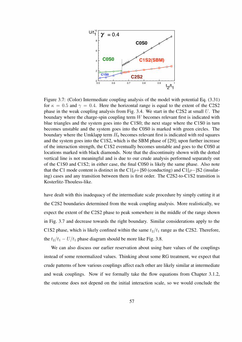
0.5 0.6 0.7 0.8 0.9 10

2

4

6

8

10

!= 0.4U/t

1

t2

/t1

C1S0

C0S0 C1S2(SBM)

C0S0

C2S2

Figure 3.7: (Color) Intermediate coupling analysis of the model with potential Eq. (3.31)for κ = 0.5 and γ = 0.4. Here the horizontal range is equal to the extent of the C2S2phase in the weak coupling analysis from Fig. 3.4. We start in the C2S2 at small U . Theboundary where the charge-spin coupling term W becomes relevant first is indicated withblue triangles and the system goes into the C1S0; the next stage where the C1S0 in turnbecomes unstable and the system goes into the C0S0 is marked with green circles. Theboundary where the Umklapp term H8 becomes relevant first is indicated with red squaresand the system goes into the C1S2, which is the SBM phase of [29]; upon further increaseof the interaction strength, the C1S2 eventually becomes unstable and goes to the C0S0 atlocations marked with black diamonds. Note that the discontinuity shown with the dottedvertical line is not meaningful and is due to our crude analysis performed separately outof the C1S0 and C1S2; in either case, the final C0S0 is likely the same phase. Also notethat the C1 mode content is distinct in the C1[ρ+]S0 (conducting) and C1[ρ−]S2 (insulat-ing) cases and any transition between them is first order. The C2S2-to-C1S2 transition isKosterlitz-Thouless-like.

have dealt with this inadequacy of the intermediate scale procedure by simply cutting it at

the C2S2 boundaries determined from the weak coupling analysis. More realistically, we

expect the extent of the C2S2 phase to peak somewhere in the middle of the range shown

in Fig. 3.7 and decrease towards the right boundary. Similar considerations apply to the

C1S2 phase, which is likely confined within the same t2/t1 range as the C2S2. Therefore,

the t2/t1 − U/t1 phase diagram should be more like Fig. 3.8.

We can also discuss our earlier reservation about using bare values of the couplings

instead of some renormalized values. Thinking about some RG treatment, we expect that

crude patterns of how various couplings affect each other are likely similar at intermediate

and weak couplings. Now if we formally take the flow equations from Chapter 3.1.2,

the outcome does not depend on the initial interaction scale, so we would conclude the

57

C2S2

C1S2

C1S0C1S0

C0S0

C0S0C0S0

???

?

0.5

U/t1

t2/t1

Figure 3.8: Schematic merging of the weak and intermediate coupling results in the modelregimes, as in Fig. 3.7, in the whole range with t2/t1 > 0.5. In weak coupling, the C2S2phase is unstable beyond the shaded region in Fig. 3.4. However, due to the crudeness ofour intermediate coupling procedure, Fig. 3.7 shows monotonic growth of the C2S2 phasewith t2/t1 past this instability. This discrepancy arises because our intermediate couplingprocedure completely ignores the spin sector. More realistically, we expect the C2S2 phaseto peak somewhere in the middle of the range shown in Fig. 3.7 and be bounded by theC1S0 for larger t2/t1. Similar considerations apply to the C1S2 phase, which is boundedby the C0S0.

C2S2 phase throughout the shaded region in Fig. 3.4. The weak coupling flow equations

miss velocity renormalizations due to chiral interactions, but these are not expected to flow

strongly and are treated reasonably in the intermediate coupling analysis. The fact that the

couplings are now finite and comparable with bare band energies is also treated reasonably

at intermediate coupling due to the power of bosonization, so the outlined forging of weak

and intermediate scales seems appropriate. Finally, the Umklapp term that is missing in

the weak coupling approach will feed into stiffening of θρ+ only, which is good for the first

instability out of the C2S2 to be into the C1S2 spin liquid.

We think that our conclusions are more robust for small γ where the extent of the C2S2

phase is larger and also the longer-ranged potential is feeding precisely into stiffening the

overall charge field θρ+, which is good for going to the C1S2 phase. On the other hand,

results at medium to large γ are likely less reliable, with different scenarios depending on

quantitative issues.

58

0.6 0.8 1 1.2 1.4 1.60

0.2

0.4

0.6

0.8

1

1.2

1.4

1.6

1.8!

t2/t1

C2S2 C1S2(SBM)

C2S2 C1S0

0.5

Figure 3.9: Same as Fig. 3.6 but for the model with interactions Eq. (3.31) truncated at the4th neighbor and starting out of the C2S2 of Fig. 3.5

3.2.3.2 Intermediate coupling phase diagram for model with potential Eq. (3.31)

truncated at the 4th neighbor

Figure 3.9 shows results of the intermediate coupling analysis for the model with interac-

tions truncated at the 4th neighbor, see Chapter 3.1.5.2. We have a rather similar story to

Fig. 3.6, except that the initial C2S2 region is bounded. Large part of the C2S2 phase exits

into the C1S2 spin liquid upon increasing interactions, and our results are probably more

robust near γ ∼ 0.2-0.3 where the C2S2 has the largest extent along the t2/t1 axis.

3.3 Summary and discussion

To summarize, in this chapter we consider electronic models for realizing spin Bose-metal

(spin liquid) phase on the two-leg triangular strip found in [29] in spin-1/2 model with ring

exchanges. We identify the SBM with the C1S2 Mott insulator of electrons.

In Chapter 3.1, we start with a two-band electron system, which is C2S2. Instead

of considering only the on-site Hubbard-type repulsion [65, 67, 68, 72, 69, 38, 73], we

study generally longer ranged density-density repulsion. This is motivated in part by the

expectation that real Coulomb interaction is not screened in Mott insulator materials, so

further neighbor repulsion can be significant, as brought up by recent ab initio work [39]

for the spin liquid material κ-(ET)2Cu2(CN)3. Using weak coupling RG analysis for the

zigzag chain problem [49, 64, 71, 65], we find that such extended interactions open much

59

wider window of the C2S2 metal compared with the Hubbard model. The main results

are shown in Fig. 3.4 and Fig. 3.5. In the first figure, we have essentially an independent

control over the Q = 0 part of the potential by allowing it to extend to far neighbors,

and we identify the dominance of VQ=0 as the main stabilizing force for the metal. In the

second figure, we truncate interactions at the 4th neighbor to check the robustness of our

conclusions, in view that such models may be easier to explore using numerical DMRG.

Our detailed quasi-1D considerations agree with the intuition that in real metals electronic

pairing instabilities are suppressed by the long-ranged piece of the Coulomb interaction.

Such widening of the C2S2 region by extending the model interaction range is warranted

if we want to bring the electronic ladder system closer to realistic situations in the 2D

candidate spin liquid materials.

In Chapter 3.2, we begin with stable C2S2 metal at weak coupling and use bosonization

to extend the analysis to intermediate coupling by gradually increasing the overall repulsion

strength. Within effective bosonic theory, we identify potential instabilities of the C2S2

phase to spin-charge interaction W(Eq. (3.47)

)and Umklapp interaction H8

(Eq. (3.49)

).

The W can drive the system into C1[ρ+]S0 phase with spin gap but still conducting along

the chain, while the Umklapp H8 can produce C1[ρ−]S2 Mott insulator with three gapless

modes, which is the desired SBM phase. We calculate the scaling dimensions of the W

and H8 terms in the harmonic theory of the C2S2 metal using bare couplings in the charge

sector and assuming stability in the spin sector—this constitutes our naive intermediate

coupling procedure. The calculation of scaling dimensions is described in Appendix 3.A

and is done numerically in the end.

We consider two cases depending on which of the termsW orH8 becomes relevant first

and apply similar intermediate coupling approach inside the resulting phase. Assuming

strong field pinning by the already relevant term, we calculate the scaling dimension of the

remaining term and estimate when it eventually drives the system into fully gapped C0S0

paramagnet (which is likely connected to the dimerized phase of the J1 − J2 Heisenberg

model at strong coupling). With the help of such admittedly crude analysis, we can map

out the phase diagram in weak to intermediate coupling regime as illustrated in schematic

Fig. 3.8 (based on more naive Fig. 3.7). Figures 3.6 and 3.9 summarize our results and

60

show where the C2S2 metal goes to the C1S2 (SBM spin liquid) upon increasing overall

repulsion strength. We conclude that the C1S2 phase is quite natural out of the wider C2S2

metallic region, in particular when driven by extended repulsive interactions. It would be

very interesting to confront our theoretical predictions with numerical DMRG studies of

such electronic models with extended repulsion.

So far, we have approached the intermediate coupling Mott insulator from the weak

coupling metallic side. One could try to attack the same problem starting from the strong

coupling limit deep in the Mott insulator where Heisenberg spin-1/2 model is appropriate.

As one nears the metallic phase, it becomes important to include multiple spin exchanges in

the effective spin Hamiltonian to better capture charge fluctuations in the underlying elec-

tron system [74, 27, 75, 76]. This is the motivation behind [29] studying J1−J2 chain with

additional four-spin ring exchanges. The concept study [29] allowed arbitrary variation

of the ring coupling compared with the Heisenberg couplings. However, coming from an

electronic model these do not vary independently and more exchange terms are also gener-

ated. It would be interesting to pursue such approach systematically studying effective spin

models with multi-spin exchanges for realistic electronic models to see if they harbor the

SBM phase. We do not make such attempts here, but only give few simple observations on

how the derivation of the spin model is modified in the presence of extended repulsion.

First of all, for the two-spin exchanges, the familiar Hubbard model expression Jrr′ =

4t2rr′/U is modified to Jrr′ = 4t2rr′/(V0 − Vr−r′). The energy denominator is not simply

the on-site U = V0 but also includes interaction potential between the two sites r and r′.

For example, [39] estimates V1/V0 ≈ 0.43 for the κ-(ET)2Cu2(CN)3 spin liquid material,

and this would significantly affect values of the exchange constants. Energy denominators

for all virtual processes are similarly affected and take a form of a charging energy for the

deviations from the background. Multispin exchange amplitudes are given by a product of

electron tunneling amplitudes for a given virtual path divided by a product of such charging

energies in intermediate states along the path. Thus, the multi-spin exchanges may in fact

be relatively more important in systems with extended interactions.

As an extreme example, imagine a very slow decrease of V (r− r′) up to some distance

R (and perhaps a faster drop thereafter). Then all exchange loops up to such radius R

61

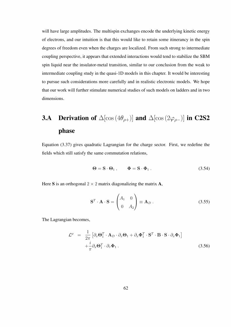
will have large amplitudes. The multispin exchanges encode the underlying kinetic energy

of electrons, and our intuition is that this would like to retain some itinerancy in the spin

degrees of freedom even when the charges are localized. From such strong to intermediate

coupling perspective, it appears that extended interactions would tend to stabilize the SBM

spin liquid near the insulator-metal transition, similar to our conclusion from the weak to

intermediate coupling study in the quasi-1D models in this chapter. It would be interesting

to pursue such considerations more carefully and in realistic electronic models. We hope

that our work will further stimulate numerical studies of such models on ladders and in two

dimensions.

3.A Derivation of ∆[cos (4θρ+)] and ∆[cos (2ϕρ−)] in C2S2

phase

Equation (3.37) gives quadratic Lagrangian for the charge sector. First, we redefine the

fields which still satisfy the same commutation relations,

Θ = S ·Θ1 , Φ = S ·Φ1 . (3.54)

Here S is an orthogonal 2× 2 matrix diagonalizing the matrix A,

ST ·A · S =

A1 0

0 A2

≡ AD . (3.55)

The Lagrangian becomes,

Lρ =1

2π

[∂xΘ

T1 ·AD · ∂xΘ1 + ∂xΦ

T1 · ST ·B · S · ∂xΦ1

]+i

π∂xΘ

T1 · ∂τΦ1 . (3.56)

62

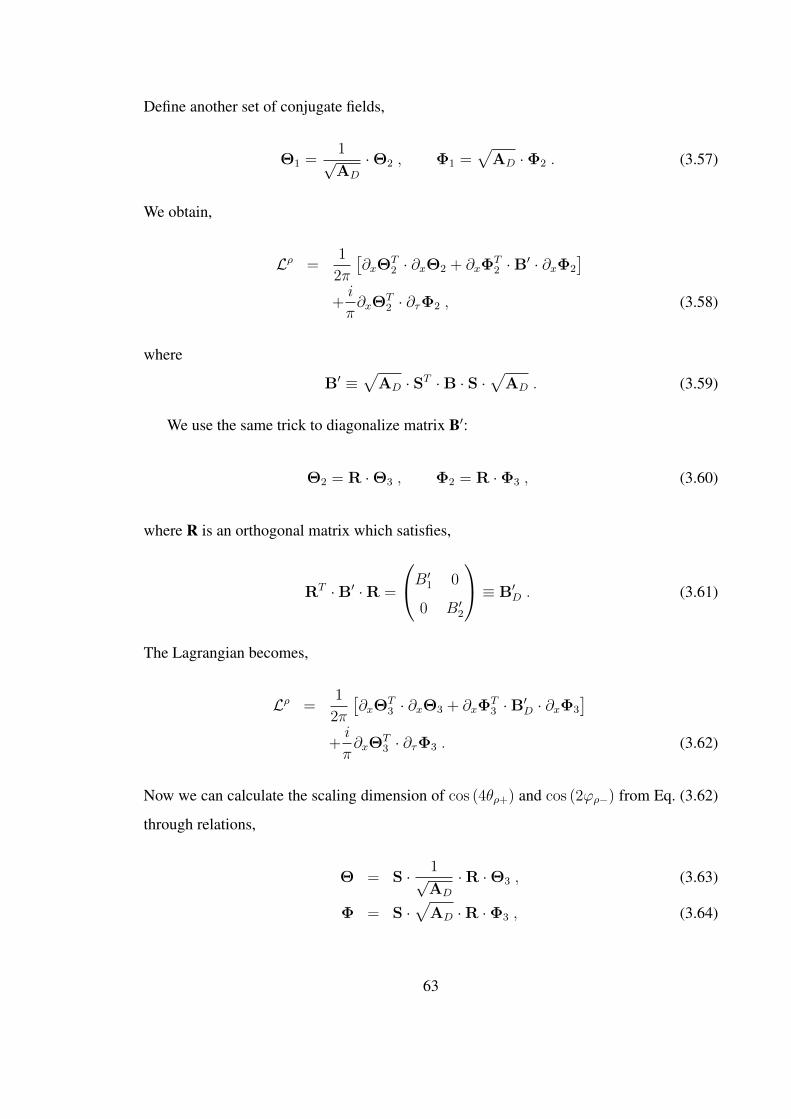
Define another set of conjugate fields,

Θ1 =1√AD

·Θ2 , Φ1 =√

AD ·Φ2 . (3.57)

We obtain,

Lρ =1

2π

[∂xΘ

T2 · ∂xΘ2 + ∂xΦ

T2 ·B′ · ∂xΦ2

]+i

π∂xΘ

T2 · ∂τΦ2 , (3.58)

where

B′ ≡√

AD · ST ·B · S ·√

AD . (3.59)

We use the same trick to diagonalize matrix B′:

Θ2 = R ·Θ3 , Φ2 = R ·Φ3 , (3.60)

where R is an orthogonal matrix which satisfies,

RT ·B′ ·R =

B′1 0

0 B′2

≡ B′D . (3.61)

The Lagrangian becomes,

Lρ =1

2π

[∂xΘ

T3 · ∂xΘ3 + ∂xΦ

T3 ·B′D · ∂xΦ3

]+i

π∂xΘ

T3 · ∂τΦ3 . (3.62)

Now we can calculate the scaling dimension of cos (4θρ+) and cos (2ϕρ−) from Eq. (3.62)

through relations,

Θ = S · 1√AD

·R ·Θ3 , (3.63)

Φ = S ·√

AD ·R ·Φ3 , (3.64)

63

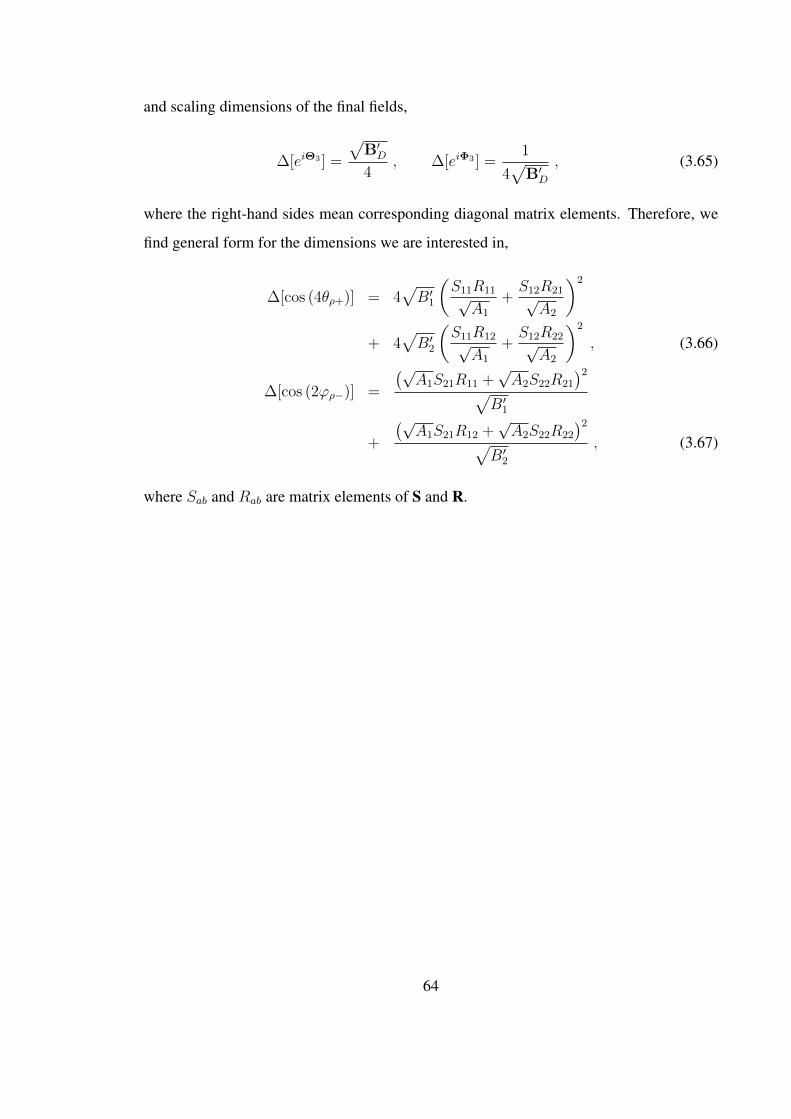
and scaling dimensions of the final fields,

∆[eiΘ3 ] =

√B′D4

, ∆[eiΦ3 ] =1

4√

B′D, (3.65)

where the right-hand sides mean corresponding diagonal matrix elements. Therefore, we

find general form for the dimensions we are interested in,

∆[cos (4θρ+)] = 4√B′1

(S11R11√

A1

+S12R21√

A2

)2

+ 4√B′2

(S11R12√

A1

+S12R22√

A2

)2

, (3.66)

∆[cos (2ϕρ−)] =

(√A1S21R11 +

√A2S22R21

)2√B′1

+

(√A1S21R12 +

√A2S22R22

)2√B′2

, (3.67)

where Sab and Rab are matrix elements of S and R.

64

Chapter 4

Effects of Zeeman field on a spinBose-metal phase

This chapter continues efforts to gain insights about the 2D spin liquid from the solvable

two-leg ladder example. Here we study the Zeeman magnetic field effects on the SBM

phase, while in a separate chapter, Chapter 5, we will study orbital field effects. One

motivation comes from experiments on the 2D spin liquid materials κ-(ET)2Cu2(CN)3 and

EtMe3Sb[Pd(dmit)2]2 measuring thermodynamic, transport, and local magnetic properties

under strong fields [15, 77, 44, 78, 17, 21]. An important question is whether the field can

induce changes in the physical state of the system.

To this end, we explore possible instabilities of the two-leg SBM state in the Zee-

man field. There have been many studies of 2D and 1D spin models under magnetic field

showing rich behaviors. For example, the phase diagram of the J1-J2 antiferromagnetic

chain with J1, J2 > 0 in the field [79, 80, 81, 82, 83] contains one-component and two-

component Luttinger liquids, a plateau, a phase with static chirality order, and a phase with

spin-nematic correlations. In the spirit of such studies, we allow a large range of fields,

which could be numerically explored in spin or electronic models realizing the SBM phase

[29, 31]. We remark that experiments on the spin liquid materials achieve only relatively

small fields—e.g., the maximum magnetization is . 0.01µB per spin. Nevertheless, some

of our two-leg ladder phases from the broader theoretical study motivate interesting 2D

states that are worth exploring.

The SBM phase on the zigzag chain can be viewed as a Gutzwiller-projected spinon

65

state where both ↑ and ↓ spinon species populate two Fermi segments (see Fig. 4.1). The

projection eliminates the overall charge mode leaving three gapless modes. We find that

this phase can in principle remain stable under the Zeeman field. We also identify all

possible instabilities out of the SBM.

Loosely speaking, the instabilities correspond to pairing of spinons separately within

each species (a kind of triplet pairing). More precisely, the relevant interactions can be

interpreted as moving a “Cooper pair” from one band to the other of the same species.

Of course, there is no long-range pairing order in the quasi-1D and in fact the dominant

correlations in our system need not be of “pair-type”—the bosonization provides the proper

treatment, while this language is only for convenience.

It can happen that the pairing is relevant for one spinon species but not the other. In

this case the system retains two gapless modes. Interestingly, spin-1 excitations become

gapped (i.e., transverse spin correlations are short-ranged), while spin-2 excitations are

gapless (i.e., nematic or two-magnon correlation functions show power law).

It can also happen that the pairing is relevant for each spinon species. In this case the

system retains only one gapless mode. Again, spin-1 excitations are gapped while spin-2

remain gapless. It further turns out that the system breaks translational symmetry and has

either period 2 valence bond solid (VBS) or period 2 static chirality order.

Such thinking about pairing within the same spinon species can be extended to 2D.

Here, if we pair only one species and not the other, we have a gap to spin-1 excitations while

at the same time we have critical spin-2 correlations and the system retains the gapless

Fermi surface for the unpaired species. On the other hand, if we have pairing within both

spinon species, the system acquires a long-range spin-nematic order. [84]

Spin-nematic phases were discovered and much discussed recently in other interest-

ing frustrated systems. For instance, such phases were found in the antiferromagnetic

zigzag ladder with easy-plane anisotropy [85] and in the ferro/antiferro zigzag ladder (J1 <

0, J2 > 0) in the Zeeman field [86, 87, 88, 89]. As for examples in 2D, spin-nematic order

was found in the frustrated square lattice with ferromagnetic J1 < 0 and antiferromagnetic

J2 > 0 and ring exchanges [90], and in the triangular lattice with ferromagnetic Heisenberg

and antiferromagnetic ring exchanges [91]. Though, many details of the nematic phases

66

proximate to the SBM studied here are of course different.

The chapter is organized as follows. In Chapter 4.1, we consider an electronic Hubbard-

type model with longer-ranged repulsion under Zeeman magnetic field and discuss the

weak coupling phase diagram in the two-band regime. We then take a leap to the Mott

insulator regime, which can be achieved from the electronic perspective by gapping out

the overall charge mode using an eight-fermion Umklapp interaction. In Chapters 4.2–4.3,

we discuss the theory and properties of the SBM under Zeeman field, and in Chapter 4.4

we consider possible instabilities and characterize the resulting phases. We conclude by

discussing generalizations of these phases to 2D.

4.1 Electrons on a two-leg zigzag strip in a Zeeman field:

Weak coupling approach

In this section, we consider half-filled electronic t1 − t2 chain with extended repulsive

interaction in the magnetic Zeeman field. The Hamiltonian is H = H0 +HZ +HV with

H0 = −∑x,α

[t1c†α(x)cα(x+ 1) + t2c

†α(x)cα(x+ 2)

+H.c.], (4.1)

HZ = −h∑x

Sz(x) , (4.2)

HV =1

2

∑x,x′

V (x− x′)n(x)n(x′) . (4.3)

Here cα(x) is a fermion annihilation operator, x is a site label on the one-dimensional (1D)

chain, and α =↑, ↓ is a spin index; n(x) ≡ c†↑(x)c↑(x) + c†↓(x)c↓(x) is electron number

on the site. Throughout, electrons are at half-filling. The Zeeman field couples to electron

spin Sz(x) ≡ 12[c†↑(x)c↑(x)− c†↓(x)c↓(x)].

In the weak coupling approach, we assume HV � H0, HZ and start with the non-

interacting band structure given by H0 +HZ and illustrated in Fig. 4.1. In this chapter, we

focus on the regime t2/t1 > 0.5 and not too large Zeeman field so that there are two occu-

67

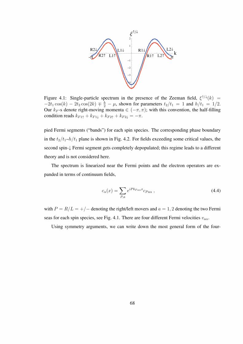
L2¯

L2­

R1¯

R1­

L1¯

L1­R2­

R2¯k

-4

-3

-2

-1

1

2

Ξ­�¯

-

Figure 4.1: Single-particle spectrum in the presence of the Zeeman field, ξ↑/↓(k) =−2t1 cos(k) − 2t2 cos(2k) ∓ h

2− µ, shown for parameters t2/t1 = 1 and h/t1 = 1/2.

Our kF -s denote right-moving momenta ∈ (−π, π); with this convention, the half-fillingcondition reads kF1↑ + kF1↓ + kF2↑ + kF2↓ = −π.

pied Fermi segments (“bands”) for each spin species. The corresponding phase boundary

in the t2/t1–h/t1 plane is shown in Fig. 4.2. For fields exceeding some critical values, the

second spin-↓ Fermi segment gets completely depopulated; this regime leads to a different

theory and is not considered here.

The spectrum is linearized near the Fermi points and the electron operators are ex-

panded in terms of continuum fields,

cα(x) =∑P,a

eiPkFaαxcPaα , (4.4)

with P = R/L = +/− denoting the right/left movers and a = 1, 2 denoting the two Fermi

seas for each spin species, see Fig. 4.1. There are four different Fermi velocities vaα.

Using symmetry arguments, we can write down the most general form of the four-

68

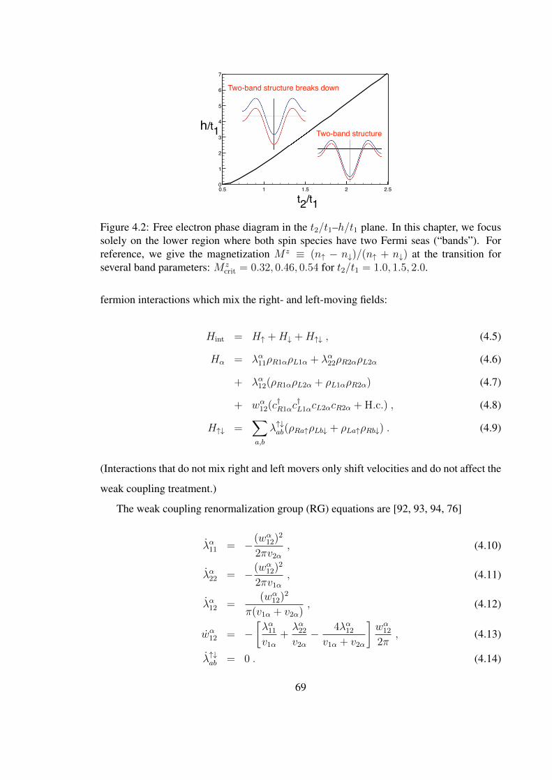
0.5 1 1.5 2 2.50

1

2

3

4

5

6

7

h/t1

t2

/t1

Two-band structure breaks down

Two-band structure

Figure 4.2: Free electron phase diagram in the t2/t1–h/t1 plane. In this chapter, we focussolely on the lower region where both spin species have two Fermi seas (“bands”). Forreference, we give the magnetization M z ≡ (n↑ − n↓)/(n↑ + n↓) at the transition forseveral band parameters: M z

crit = 0.32, 0.46, 0.54 for t2/t1 = 1.0, 1.5, 2.0.

fermion interactions which mix the right- and left-moving fields:

Hint = H↑ +H↓ +H↑↓ , (4.5)

Hα = λα11ρR1αρL1α + λα22ρR2αρL2α (4.6)

+ λα12(ρR1αρL2α + ρL1αρR2α) (4.7)

+ wα12(c†R1αc†L1αcL2αcR2α + H.c.) , (4.8)

H↑↓ =∑a,b

λ↑↓ab(ρRa↑ρLb↓ + ρLa↑ρRb↓) . (4.9)

(Interactions that do not mix right and left movers only shift velocities and do not affect the

weak coupling treatment.)

The weak coupling renormalization group (RG) equations are [92, 93, 94, 76]

λα11 = −(wα12)2

2πv2α

, (4.10)

λα22 = −(wα12)2

2πv1α

, (4.11)

λα12 =(wα12)2

π(v1α + v2α), (4.12)

wα12 = −[λα11

v1α

+λα22

v2α

− 4λα12

v1α + v2α

]wα12

2π, (4.13)

λ↑↓ab = 0 . (4.14)

69

Here O ≡ dO/d`, where ` is logarithm of the length scale; α =↑, ↓; and a, b ∈ {1, 2}. We

see that the terms λ↑↓ab do not flow and the two spin species behave independently from each

other in the weak coupling regime.

We therefore focus on one species at a time. Effectively, this is equivalent to a two-

band model of spinless fermions in one dimensions [92, 93, 94, 76] in the absence of any

Umklapps. The RG Eqs. (4.10)–(4.13) have the Kosterlitz-Thouless form and can be solved

exactly. We define

yα ≡ λα11

2πv1α

+λα22

2πv2α

− 2λα12

π(v1α + v2α). (4.15)

Eqs. (4.10)–(4.13) simplify,

yα = −(v1α + v2α)2 + 4v1αv2α

2π2v1αv2α(v1α + v2α)2(wα12)2 , (4.16)

wα12 = −yαwα12 . (4.17)

The wα12 renormalizes to zero if the bare couplings satisfy

yα(` = 0) ≥

√(v1α + v2α)2 + 4v1αv2α

2π2v1αv2α(v1α + v2α)2|wα12(` = 0)| . (4.18)

In this case, the two-band state of species α is stable and gives two gapless modes.

On the other hand, if the condition Eq. (4.18) is not satisfied, then wα12 runs to strong

coupling. In this case, only one gapless mode remains. To analyze this, we bosonize

cPaα ∼ ηaαei(ϕaα+Pθaα) , (4.19)

with canonically conjugate boson fields:

[ϕaα(x), ϕbβ(x′)] = [θaα(x), θbβ(x′)] = 0 , (4.20)

[ϕaα(x), θbβ(x′)] = iπδabδαβ Θ(x− x′) , (4.21)

where Θ(x) is the heaviside step function. Here we use Majorana fermions ({ηaα, ηbβ} =

70

2δabδαβ) as Klein factors, which assure that the fermion fields with different flavors anti-

commute with one another.

For convenience, we introduce

θ±α ≡ θ1α ± θ2α√2

, α =↑ or ↓ , (4.22)

θρ+ ≡θ+↑ + θ+

↓√2

=θ1↑ + θ2↑ + θ1↓ + θ2↓

2, (4.23)

θσ+ ≡θ+↑ − θ

+↓√

2=θ1↑ + θ2↑ − θ1↓ − θ2↓

2, (4.24)

and similarly for ϕ variables. The wα12 term becomes

wα12(c†R1αc†L1αcL2αcR2α + H.c.) ∼ wα12 cos(2

√2ϕ−α ) . (4.25)

When wα12 is relevant and flows to large values, it pins the difference field ϕ−α , while the

overall field ϕ+α remains gapless (as it should, since the α-electrons have an incommen-

surate conserved density and there are no four-fermion Umklapps). In this phase, the α-

electron operator becomes gapped. Pair-α-electron operator is gapless, and also specific

particle-hole composites are gapless, with details depending on the sign of wα12. We are

primarily interested in repulsively interacting electrons and expect the particle-hole ob-

servables to be more prominent, although not dramatically since for too strong repulsion

the conducting state of the ↑ and ↓ electrons is destroyed towards Mott insulator as de-

scribed below. We do not provide more detailed characterization of the conducting phases

of electrons here, as we are eventually interested in the Mott insulating regime where the ↑

and ↓ species become strongly coupled. (The two-band spinless electron system was con-

sidered, e.g., in [92, 93, 94, 76], and our analysis in Chapter 4.3 can be readily tailored to

the electronic phases here.)

In the model with longer-ranged density–density repulsion, Eq. (4.3), the bare couplings

71

are

λα11 = VQ=0 − V2kF1α, (4.26)

λα22 = VQ=0 − V2kF2α, (4.27)

λα12 = VQ=0 − VkF1α+kF2α, (4.28)

wα12 = VkF1α−kF2α− VkF1α+kF2α

, (4.29)

λ↑↓ab = VQ=0 . (4.30)

Here VQ ≡∑∞

x′=−∞ V (x− x′)eiQ(x−x′) = V−Q.

As an example, we consider the following potential:

V (x− x′) =

U , |x− x′| = 0

κUe−γ|x−x′| , |x− x′| ≥ 1

. (4.31)

This was used in [31] to provide stable realizations of the C2S2 metal and the SBM Mott

insulator of electrons in zero field. Here U is the overall energy scale and also the on-

site repulsion; dimensionless parameter κ controls the relative strength of further-neighbor

interactions; and γ defines the decay rate. Applying the stability condition, Eq. (4.18), we

can now determine the phase diagram in the weak coupling approach in the regime where

the kinetic energy gives four modes.

Figure 4.3 provides an illustration for γ = 0.3 and κ = 0.5. The w↑12 interaction is

relevant in the region with hash lines at roughly 45 degrees and the w↓12 is relevant in the

region with hash lines at 135 degrees with respect to the horizontal axis. There are four

distinct phases. First, when both w↑12 and w↓12 are irrelevant, we have a phase with four

gapless modes, which is connected to the C2S2 phase at h = 0. (Note, however, that we

assumed HZ � HV , so the formal h → 0 limit here is different from the weak coupling

analysis at h = 0 in [65, 31].)

Next, when w↑12 is relevant while w↓12 is irrelevant, we have a phase with three gapless

modes: one associated with the ↑-electrons and two associated with the ↓-electrons. In this

phase, inserting a single ↑-electron costs a finite gap while inserting a pair of ↑-electrons

72

0.5 1 1.5 2 2.50

1

2

3

4

5

6

7 Boundary of relevant

Boundary of relevant

Boundary of two-band structure

h/t1

t2/t1

ɤ=0.3; ϰ=0.5

Different Theory

(C2S2)

w12

w12

3 gapless

modes

2 gapless

modes

2 gapless charge modes

and 2 gapless spin modes

3 gapless

modes

Figure 4.3: An example of the weak-coupling phase diagram in the electron system underthe Zeeman field, using model interactions Eq. (4.31) with κ = 0.5 and γ = 0.3. Wefocus on the region where the kinetic energy gives four modes (see Figs. 4.1, 4.2) and findfour phases: metallic phase with four gapless modes evolving out of the C2S2 phase inzero field; phase with three gapless modes where only the w↑12-term is relevant and flowsto strong coupling; phase with three gapless modes where only the w↓12-term is relevant;and phase with two gapless modes where both the w↑12 and w↓12 are relevant. The w↑12-termis relevant in the region with hash lines at roughly 45 degrees and the w↓12-term is relevantin the region with hash lines at 135 degrees with respect to the horizontal axis. Note thatthe w↓12-term always becomes relevant upon approaching the boundary of the two-bandstructure [76].

or a particle-hole combination of ↑-electrons is gapless. The ↓ electrons are completely

gapless.

When w↓12 is relevant while w↑12 is irrelevant, we have another phase with three gapless

modes, which is similar to the preceding paragraph but with ↑ and ↓ interchanged. As can

be seen in Fig. 4.3, w↓12 is always relevant when h approaches the critical value, [76] and

the instability arises because the v2↓ approaches zero.

Finally, for large t2/t1, bothw↑12 andw↓12 are relevant and we have a phase with only two

gapless modes: one associated with spin-↑ and the other with spin-↓ species. In this case,

inserting a single electron of either spin is gapped, while inserting a pair or a particle-hole

combination of same-spin electrons is gapless.

73

4.2 Transition to Mott insulator: SBM phase

Note that all phases accessed from the weak coupling analysis are conducting along the

zigzag chain. Mott insulating states do not appear since there is no four-fermion Umklapp.

The half-filled system does become insulating for sufficiently strong repulsion. This can be

achieved by including a valid eight-fermion Umklapp, which is irrelevant at weak coupling

but can become relevant at intermediate to strong coupling [29, 31]:

H8 = v8(c†R1↑c†R1↓c

†R2↑c

†R2↓cL1↑cL1↓cL2↑cL2↓ + H.c.)

∼ 2v8 cos(4θρ+) , (4.32)

where θρ+ is defined in Eq. (4.23) and describes slowly varying electron density, ρe(x) =

2∂xθρ+/π. The density–density repulsion gives coarse-grained interactionHint ∼ VQ=0(∂xθρ+)2.

This will stiffen the θρ+ field and will reduce the scaling dimension of the Umklapp term.

For sufficiently strong repulsion the Umklapp becomes relevant and will grow at long

scales, pinning the θρ+ and driving a metal-insulator transition. As discussed in [29, 31],

we expect that Mott insulator corresponding to a spin model with spins residing on sites is

described by v8 > 0 and the pinning condition

4θ(0)ρ+ = π (mod 2π) . (4.33)

Such gapping out of the overall charge mode can occur out of any of the four conducting

phases discussed in Fig. 4.3. When this happens out of the four-mode metal, we obtain

spin liquid Mott insulator with three gapless modes—the spin Bose-metal. In principle,

one could perform an intermediate coupling analysis similar to that in [31] to estimate the

strength of the repulsion needed to drive the metal-insulator transition, but we will not try

this here. Below we discuss qualitatively the stability and physical observables in the SBM

phase under the Zeeman field. We will then consider instabilities of the SBM similar to the

wα12-driven transitions out of the four-mode metal above, but now with the ↑ and ↓ systems

strongly coupled to form the Mott insulator.

Reference [29] also presented another route to describe the SBM in a spin-only model

74

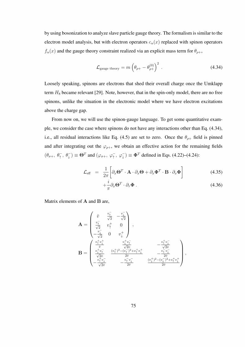
by using bosonization to analyze slave particle gauge theory. The formalism is similar to the

electron model analysis, but with electron operators cα(x) replaced with spinon operators

fα(x) and the gauge theory constraint realized via an explicit mass term for θρ+,

Lgauge theory = m(θρ+ − θ(0)

ρ+

)2

. (4.34)

Loosely speaking, spinons are electrons that shed their overall charge once the Umklapp

termH8 became relevant [29]. Note, however, that in the spin-only model, there are no free

spinons, unlike the situation in the electronic model where we have electron excitations

above the charge gap.

From now on, we will use the spinon-gauge language. To get some quantitative exam-

ple, we consider the case where spinons do not have any interactions other than Eq. (4.34),

i.e., all residual interactions like Eq. (4.5) are set to zero. Once the θρ+ field is pinned

and after integrating out the ϕρ+, we obtain an effective action for the remaining fields

(θσ+, θ−↑ , θ

−↓ ) ≡ ΘT and (ϕσ+, ϕ

−↑ , ϕ

−↓ ) ≡ ΦT defined in Eqs. (4.22)–(4.24):

Leff =1

2π

[∂xΘ

T ·A · ∂xΘ + ∂xΦT ·B · ∂xΦ

](4.35)

+i

π∂xΘ

T · ∂τΦ . (4.36)

Matrix elements of A and B are,

A =

v

v−↑√2− v−↓√

2v−↑√

2v+↑ 0

− v−↓√2

0 v+↓

,

B =

v+↑ v

+↓

v

v+↓ v−↑√

2v−v+↑ v

−↓√

2vv+↓ v

−↑√

2v

(v+↑ )2−(v−↑ )2+v+↑ v+↓

2v−v−↑ v

−↓

2v

−v+↑ v−↓√

2v−v−↑ v

−↓

2v

(v+↓ )2−(v−↓ )2+v+↑ v+↓

2v

,

75

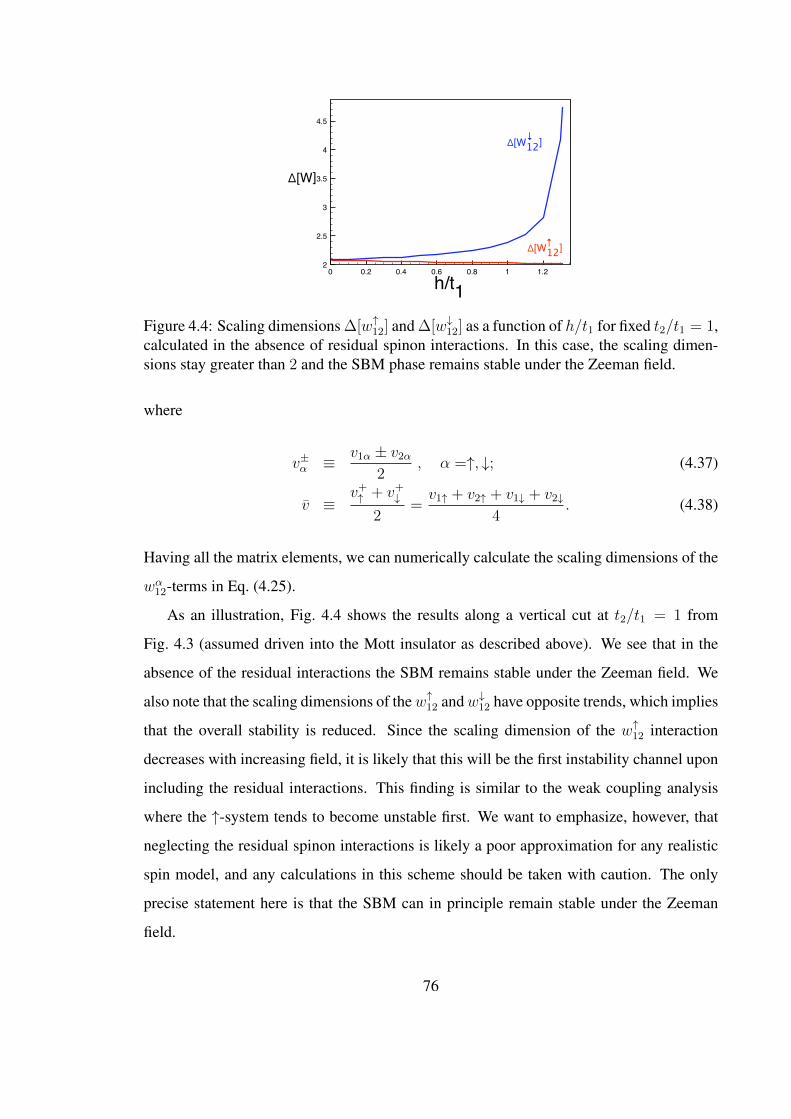
0 0.2 0.4 0.6 0.8 1 1.22

2.5

3

3.5

4

4.5

Δ[W12]

Δ[W12]

h/t1

Δ[W]

↑

↓

Figure 4.4: Scaling dimensions ∆[w↑12] and ∆[w↓12] as a function of h/t1 for fixed t2/t1 = 1,calculated in the absence of residual spinon interactions. In this case, the scaling dimen-sions stay greater than 2 and the SBM phase remains stable under the Zeeman field.

where

v±α ≡ v1α ± v2α

2, α =↑, ↓; (4.37)

v ≡v+↑ + v+

↓

2=v1↑ + v2↑ + v1↓ + v2↓

4. (4.38)

Having all the matrix elements, we can numerically calculate the scaling dimensions of the

wα12-terms in Eq. (4.25).

As an illustration, Fig. 4.4 shows the results along a vertical cut at t2/t1 = 1 from

Fig. 4.3 (assumed driven into the Mott insulator as described above). We see that in the

absence of the residual interactions the SBM remains stable under the Zeeman field. We

also note that the scaling dimensions of thew↑12 andw↓12 have opposite trends, which implies

that the overall stability is reduced. Since the scaling dimension of the w↑12 interaction

decreases with increasing field, it is likely that this will be the first instability channel upon

including the residual interactions. This finding is similar to the weak coupling analysis

where the ↑-system tends to become unstable first. We want to emphasize, however, that

neglecting the residual spinon interactions is likely a poor approximation for any realistic

spin model, and any calculations in this scheme should be taken with caution. The only

precise statement here is that the SBM can in principle remain stable under the Zeeman

field.

76

In Chapter 4.4 we discuss phases proximate to the SBM. Motivated by the above ob-

servations, we will consider first the case where only the w↑12 term becomes relevant; we

will also consider the situation where both w↑12 and w↓12 are relevant. Before this, we need

to describe main physical observables in the SBM under the Zeeman field, which we will

then use to analyze the instabilities and the properties of the resulting phases.

4.3 Observables in the SBM in Zeeman field

In the presence of the Zeeman field, the system has Sztot spin conservation symmetry and

complex conjugation symmetry (C : i → −i) in the Sz basis. The system also has lattice

translation and inversion (I : x → −x) symmetries. The internal symmetries are suffi-

ciently reduced compared with the SU(2)-invariant case of [29] that we need to revisit the

physical observables in the SBM.

We first consider Sz-conserving bilinears, which we will also call “spin-0” objects,

ε2kFaα ≡ f †LaαfRaα , (4.39)

εkF1α+kF2α≡ 1

2

(f †L1αfR2α + f †L2αfR1α

), (4.40)

χkF1α+kF2α≡ 1

2

(f †L1αfR2α − f †L2αfR1α

), (4.41)

εkF1α−kF2α≡ 1

2

(f †L1αfL2α + f †R2αfR1α

), (4.42)

χkF1α−kF2α≡ 1

2

(f †L1αfL2α − f †R2αfR1α

), (4.43)

(no summation over a or α). We define ε−Q = ε†Q and χ−Q = χ†Q so that ε(x) and χ(x) are

Hermitian operators.

The ε bilinears appear, e.g., when expressing spinon hopping energies, while the χ

bilinears appear in currents. Specifically, consider a bond [x, x+ n],

B(n)(x) ∼ f †α(x)fα(x+ n) + H.c. , (4.44)

J (n)(x) ∼ i[f †α(x)fα(x+ n)− H.c.

], (4.45)

77

where α =↑ or ↓ species can come with independent amplitudes. Expansion in terms of

the continuum fields gives, up to real factors,

B(n)Q ∼ einQ/2εQ , (4.46)

J (n)Q ∼ einQ/2χQ . (4.47)

Note that we can view ε(x) as a site-centered energy operator, e.g., ε(x) ∼ B(1)(x−1)+

B(1)(x) ∼ B(2)(x − 1), in the sense of having the same symmetry properties. We can also

view ε(x) ∼ Sz(x) in the same sense because of the presence of the Zeeman energy. [More

generally, the symmetry properties of any operator are not changed upon multiplying by

Sz(x).] On the other hand, the bond operator B(n)(x) has the same symmetry properties as

a bond energy such as ~S(x) · ~S(x+ n) and can be used to characterize VBS correlations in

the spin system.

Similarly, we can view χ(x) as a site-centered current, χ(x) ∼ J (1)(x−1)+J (1)(x) ∼

J (2)(x−1), and also as a scalar chirality, χ(x) ∼ ~S(x−1) · ~S(x)× ~S(x+1), while J (n)(x)

has the same symmetry properties as a spin current, J (n)(x) ∼ i[S+(x)S−(x+ n)−H.c.].

Symmetry analysis shows that εQ transforms to ε−Q under either lattice inversion I or

complex conjugation C, while χQ transforms to −χ−Q under either I or C. We can then

give an independent argument for the relations Eqs. (4.46) and (4.47) for Q 6= 0, π, and can

show generally that, up to complex phase factors, such εQ and χQ cover all independent

spin-0 observables for the system in the Zeeman field.

Special care is needed for Q = π. In this case, Eqs. (4.46) and (4.47) hold only for

n = even. On the other hand, B(n=odd)π is odd under inversion I and even under complex

conjugation C, while J (n=odd)π is even under I and odd under C. In particular, the nearest-

neighbor bond B(1)π and J (1)

π are independent observables from επ ∼ B(2)π and χπ ∼ J (2)

π .

In the present SBM problem, such Q = π observables do not appear as bilinears but appear

as four-fermion terms below.

78

The bosonized expressions for the spin-0 bilinears are:

ε2kFaα = iei(θρ++αθσ++a√

2θ−α ) , (4.48)

εkF1α+kF2α= −iη1αη2αe

i(θρ++αθσ+) sin(√

2ϕ−α ) , (4.49)

χkF1α+kF2α= η1αη2αe

i(θρ++αθσ+) cos(√

2ϕ−α ) , (4.50)

εkF1α−kF2α= −iη1αη2αe

i√

2θ−α sin(√

2ϕ−α ) , (4.51)

χkF1α−kF2α= η1αη2αe

i√

2θ−α cos(√

2ϕ−α ) , (4.52)

where we used definitions Eqs. (4.22)–(4.24) and α = +/− for spin ↑ or ↓ and a = +/−

for band 1 or 2.

To bring out the wavevector Q = π that will play an important role in the analysis of

phases near the SBM, we need to consider four-fermion terms. We find,

B(1)π : i(εkF1↑+kF2↑εkF1↓+kF2↓ − H.c.) ∼ (4.53)

∼ Γ sin(√

2ϕ−↑ ) sin(√

2ϕ−↓ ) sin(2θρ+); (4.54)

i(χkF1↑+kF2↑χkF1↓+kF2↓ − H.c.) ∼ (4.55)

∼ Γ cos(√

2ϕ−↑ ) cos(√

2ϕ−↓ ) sin(2θρ+); (4.56)

and also

χπ : εkF1↑+kF2↑χkF1↓+kF2↓ + H.c. ∼ (4.57)

∼ Γ sin(√

2ϕ−↑ ) cos(√

2ϕ−↓ ) sin(2θρ+); (4.58)

χkF1↑+kF2↑εkF1↓+kF2↓ + H.c. ∼ (4.59)

∼ Γ cos(√

2ϕ−↑ ) sin(√

2ϕ−↓ ) sin(2θρ+) . (4.60)

Here Γ ≡ η1↑η1↓η2↑η2↓. Note that we have only listed observables containing sin(2θρ+).

The other independent spin-0 objects επ and J (1)π contain cos(2θρ+) and vanish because of

the pinning condition Eq. (4.33).

Having discussed Sz-conserving observables, we can similarly consider Sz-raising ob-

79

servables. We will call objects corresponding to δSz = 1 or 2 as “spin-1” or “spin-2”,

respectively. We have spin-1 bilinears,

S+−PkFa↑+P ′kFb↓ ≡ f †Pa↑fP ′b↓ . (4.61)

Generically, these all carry different momenta. We can readily write bosonized expressions.

For reference, we give the main ones that contain oppositely moving fields:

S+kFa↑+kFb↓

= ηa↑ηb↓ e−i[ϕσ++ 1√

2(aϕ−↑ −bϕ

−↓ )]

× ei[θρ++ 1√

2(aθ−↑ +bθ−↓ )]

, (4.62)

where we used convention a, b = +/− for band 1 or 2. We can generally argue that at

Q 6= 0, π, objects S+Q that transform like Fourier modes of the S+(x) operator cover, up to

complex phases, all distinct spin-1 observables. In the present SBM system, we do not find

any interesting spin-1 observables at Q = 0, π.

Since we will encounter phases where S+ is gapped, we also need to consider δSz = 2

observables, i.e., some kind of “magnon pair” creation operators. Because of the hard spin

condition, we define them on bonds [x, x+ n],

P+,(n)(x) ≡ S+(x)S+(x+ n) (4.63)

∼ f †↑(x)f †↑(x+ n)f↓(x+ n)f↓(x) . (4.64)

The last line can be expanded in terms of the continuum fields and organized as follows.

For α-species, a “pair” operator f †α(x)f †α(x + n) contains zero momentum contributions

f †Raαf†Laα, a = 1 or 2; ±(kF1α + kF2α) momentum contributions f †P1αf

†P2α, P = L/R;

and ±(kF1α − kF2α) contributions f †P1αf†−P2α. Multiplying the pair creation operator for ↑

species and pair destruction operator for ↓ species, we obtain contributions to P+ carrying

combinations of the above momenta.

We can argue on general symmetry grounds that, up to complex phases, there is a

single independent spin-2 object at Q 6= 0, π. On the other hand, at Q = π there are two

80

independent objects that transform differently under lattice inversion; they can be realized

by P+,(n=even)π and P+,(n=odd)

π respectively. At Q = 0, we consider only objects P+,(n)Q=0

which have the same symmetry properties for any n.

In the present SBM problem, the main spin-2 observables occur precisely at Q = 0, π,

and we give bosonized expressions only for these. ForQ = 0, there are four possible terms:

P+,(n)Q=0 : f †Ra↑f

†La↑fLb↓fRb↓ ∼ e−i[2ϕσ++

√2(aϕ−↑ −bϕ

−↓ )] (4.65)

with independent a, b = +/− corresponding to bands 1 or 2. For Q = π we find

P+,(n)Q=π ∼ f †R1↑f

†R2↑fL2↓fL1↓e

iπn2 +f †L1↑f

†L2↑fR2↓fR1↓e

−iπn2

∼ Γ e−i2ϕσ+ sin[2θρ+ +

π

2(n− 1)

]. (4.66)

Because of the pinning condition on the θρ+, only the P+,(n=odd)Q=π are nonzero, and we can

use the nearest-neighbor magnon-pair operator P+,(1) as the main representative.

4.4 Nearby phases out of the SBM in the field

We now consider what happens when either w↑12 or w↓12 from Eq. (4.25) or both become

relevant.

4.4.1 Phases when w↑12 is relevant

Let us start with the case when the w↑12 term is relevant while w↓12 is irrelevant. The field ϕ−↑

is pinned, while fields ϕ−↓ and ϕσ+ remain gapless, so we have two gapless modes. There

is no static order. We summarize characteristic power law observables in Table 4.1 and

discuss them in turn.

First, all observables εQ and χQ in Eqs. (4.48)–(4.52) constructed out of the f↓ fields

show power law. On the other hand, such observables constructed out of the f↑ fields that

contain θ−↑ become short-ranged once we pin the conjugate ϕ−↑ ; thus, onlyQ = kF1↑+kF2↑

81

can remain power law. There are two cases depending on the sign of w↑12:

w↑12 > 0 : ϕ−↑ =(2n+ 1)π

2√

2, n ∈ Z , (4.67)

εkF1↑+kF2↑ ∼ eiθσ+ , χkF1↑+kF2↑ = 0; (4.68)

w↑12 < 0 : ϕ−↑ =2nπ

2√

2, n ∈ Z , (4.69)

χkF1↑+kF2↑ ∼ eiθσ+ , εkF1↑+kF2↑ = 0 . (4.70)

Next, note that all spin-1 observables S+Q become short-ranged since they all contain

the wildly fluctuating field θ−↑ . Schematically, the individual f↑ become gapped because of

their “pairing”. On the other hand, spin-2 observables contain pairs of f↑ and can remain

gapless. Explicitly, after pinning the ϕ−↑ , we have for the dominant correlations at Q = 0

and π

P+Q=0 ∼ e−i2ϕσ+e±i

√2ϕ−↓ , (4.71)

P+,(1)Q=π ∼ e−i2ϕσ+ . (4.72)

The gaplessness of the ϕσ+ is required since Sztot is conserved and incommensurate with

the lattice. We can map the spin system to hard-core bosons, [88] and in the present case

single boson excitations are gapped, while pair boson excitations are gapless and created by

ei2ϕσ+ . . . . In the “particle-hole” sector, we have strong “density” or “current” correlations,

Eq. (4.68) or (4.70), at wavelengths that can be related to typical separations between boson

pairs, and such eiθσ+ contribution is generally expected in a Luttinger liquid of pairs. Thus,

the resulting state has spin-nematic power law correlations as well as density or current

power law correlations. Which one is dominant depends on the scaling dimensions of

ei2ϕσ+ versus eiθσ+ . The scaling dimensions would need to be calculated numerically since

the ϕσ+ and ϕ−↓ mix in general; we do not attempt such quantitative estimates here.

Having discussed observables controlled by the gapless σ+ part, let us finally mention

that B(1)π and χπ directly detect the gapless ϕ−↓ field, cf. Eqs. (4.53)–(4.60). In the phase

discussed in this section they have the same power law decays.

We have considered the case when only w↑12 becomes relevant. The case when only w↓12

82

Pinned ϕ−↑ : Common power-law order for either sign of w↑12

ε±2kFa↓

ε±(kF1↓+kF2↓); ε±(kF1↓−kF2↓); B(1)π ; P+

{Q}χ±(kF1↓+kF2↓) χ±(kF1↓−kF2↓) χπ

Distinct power law correlationsw↑12 > 0 : ε±(kF1↑+kF2↑)

w↑12 < 0 : χ±(kF1↑+kF2↑)

Table 4.1: Summary of the main observables when w↑12 term is relevant and pins ϕ−↑ . Crit-ical wavevectors Q for the magnon-pair creation operator are obtained by combining anyof q↑ = {0, ± (kF1↑ + kF2↑)} with any of q↓ = {0, ± (kF1↓ + kF2↓), ± (kF1↓ − kF2↓)},Q = q↑ + q↓; the most important ones are Q = 0 and π.

becomes relevant can be treated similarly by interchanging ↑ and ↓.

4.4.2 Phases when both w↑12 and w↓12 are relevant

Let us now discuss the phases out of the SBM when both w↑12 and w↓12 terms get relevant.

Once the couplings flow to large values, both variables ϕ−↑ and ϕ−↓ will be pinned so as to

minimize the energy. There are four possible situations depending on the signs of the w↑12

and w↓12.

In all cases, we find that the translational symmetry is broken by either a static order in

Bπ (corresponding to period-2 valence bond solid) or χπ (corresponding to period-2 chiral-

ity order). Coexisting with this, we have one gapless mode, namely the overall spin mode

“σ+”, which must remain gapless as long as the magnetization density is incommensurate

with the lattice. Similarly to the case with one relevant coupling, spin-1 observables are

gapped. Spin-2 observables are gapless, with the dominant contributions

P+Q=0 ∼ P

+Q=π ∼ e−i2ϕσ+ . (4.73)

(Note that the original wavevectors Q = 0 and π are not distinguishable once we have the

period-2 static orders.) Together with such spin-nematic observables, we also have spin-

0 observables of the ε- or χ-type depending on the pinning details, with the wavevectors

±(kF1α + kF2α) which satisfy kF1↑ + kF2↑ = −(kF1↓ + kF2↓)− π.

Below, we consider four different pinning situations in more details. The main features

83

w↑12 w↓12 Static Order Power-Law Correlations+ + B(1)

π ε±(kF1α+kF2α) P+{Q}

- - B(1)π χ±(kF1α+kF2α) P+

{Q}

+ - χπε±(kF1↑+kF2↑); P+

{Q}χ±(kF1↓+kF2↓)

- + χπε±(kF1↓+kF2↓); P+

{Q}χ±(kF1↑+kF2↑)

Table 4.2: Summary of the cases when bothw↑12 andw↓12 terms are relevant. Forw↑12w↓12 > 0

we have period-2 VBS order, while for w↑12w↓12 < 0 we have period-2 chirality order. In

all cases, coexisting with such static order, we have power law correlations in the spin-2(magnon pair) observable P+ and in the specific ε/χ observables.

in each case are summarized in Table 4.2.

4.4.2.1 w↑12 > 0, w↓12 > 0

The pinning conditions for fields ϕ−↑ and ϕ−↓ are

ϕ−↑ =(2n+ 1)π

2√

2, ϕ−↓ =

(2m+ 1)π

2√

2, n,m ∈ Z . (4.74)

In this case, B(1)π obtains an expectation value while χπ = 0. Thus we expect to see period-2

VBS order as illustrated in Fig. 4.5. We also have power law correlations in

εkF1↑+kF2↑ ∼ ε−kF1↓−kF2↓ ∼ eiθσ+ , (4.75)

while χkF1α+kF2α= 0. Note that because of the relation Eq. (4.53) [in the sense that

i(εkF1↑+kF2↑εkF1↓+kF2↓ − H.c.) has the same symmetry properties as B(1)π ], once the system

develops static order in B(1)π , the εkF1↑+kF2↑ and ε−kF1↓−kF2↓ = ε†kF1↓+kF2↓

are no longer

independent. Appropriately, the wavevectors kF1↑+kF2↑ and−kF1↓−kF2↓ differ by π and

also become connected.

84

Figure 4.5: Picture of the valence bond solid order when B(1)π gains an expectation value.

Top: 1D chain view. Bottom: the same in two-leg ladder view. Coexisting with the staticorder, we also have spin-nematic power law correlations and power law in either ε or χchannels (these properties are not depicted in any way).

4.4.2.2 w↑12 < 0, w↓12 < 0

Here, the pinning conditions are

ϕ−↑ =2nπ

2√

2, ϕ−↓ =

2mπ

2√

2, n,m ∈ Z . (4.76)

Again, B(1)π obtains an expectation value while χπ = 0. However, here we have power law

correlations in

χkF1↑+kF2↑ ∼ χ−kF1↓−kF2↓ ∼ eiθσ+ (4.77)

while εkF1α+kF2α= 0. Similar to the discussion in the preceding case and using relation

Eq. (4.55), χkF1↑+kF2↑ and χ−kF1↓−kF2↓ are not independent observables in the presence of

the static order in B(1)π .

4.4.2.3 w↑12 > 0, w↓12 < 0

In this case, the pinning conditions are

ϕ−↑ =(2n+ 1)π

2√

2, ϕ−↓ =

2mπ

2√

2, n,m ∈ Z . (4.78)

In this phase, χπ obtains an expectation value while B(1)π = 0. Thus we expect to see

period-2 chirality order as illustrated in Fig. 4.6. We also have power law correlations in

εkF1↑+kF2↑ ∼ χ−kF1↓−kF2↓ ∼ eiθσ+ , (4.79)

85

+ - + + + + + ++ - - - - - -

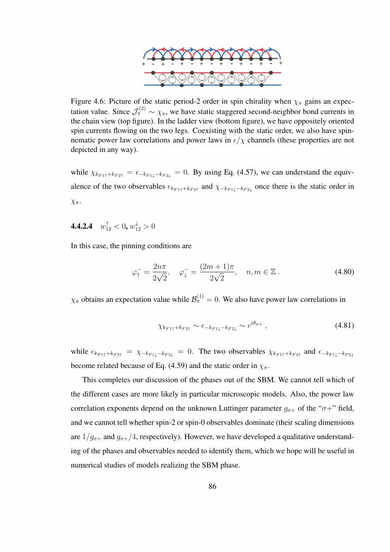
Figure 4.6: Picture of the static period-2 order in spin chirality when χπ gains an expec-tation value. Since J (2)

π ∼ χπ, we have static staggered second-neighbor bond currents inthe chain view (top figure). In the ladder view (bottom figure), we have oppositely orientedspin currents flowing on the two legs. Coexisting with the static order, we also have spin-nematic power law correlations and power laws in ε/χ channels (these properties are notdepicted in any way).

while χkF1↑+kF2↑ = ε−kF1↓−kF2↓ = 0. By using Eq. (4.57), we can understand the equiv-

alence of the two observables εkF1↑+kF2↑ and χ−kF1↓−kF2↓ once there is the static order in

χπ.

4.4.2.4 w↑12 < 0, w↓12 > 0

In this case, the pinning conditions are

ϕ−↑ =2nπ

2√

2, ϕ−↓ =

(2m+ 1)π

2√

2, n,m ∈ Z . (4.80)

χπ obtains an expectation value while B(1)π = 0. We also have power law correlations in

χkF1↑+kF2↑ ∼ ε−kF1↓−kF2↓ ∼ eiθσ+ , (4.81)

while εkF1↑+kF2↑ = χ−kF1↓−kF2↓ = 0. The two observables χkF1↑+kF2↑ and ε−kF1↓−kF2↓

become related because of Eq. (4.59) and the static order in χπ.

This completes our discussion of the phases out of the SBM. We cannot tell which of

the different cases are more likely in particular microscopic models. Also, the power law

correlation exponents depend on the unknown Luttinger parameter gσ+ of the “σ+” field,

and we cannot tell whether spin-2 or spin-0 observables dominate (their scaling dimensions

are 1/gσ+ and gσ+/4, respectively). However, we have developed a qualitative understand-

ing of the phases and observables needed to identify them, which we hope will be useful in

numerical studies of models realizing the SBM phase.

86

4.5 Discussion

In this chapter, we studied instabilities of the two-leg SBM under the Zeeman magnetic

field. The instabilities are driven by the wα12 interactions, Eq. (4.8), and we analyzed pos-

sible outcomes using Bosonization. In all cases, we found a gap to spin-1 excitations,

while spin-nematic (two-magnon) correlations are power law. Loosely speaking, this ap-

pears because of some pairing of spinons, while the precise characterization is obtained by

analyzing all physical observables.

Here we want to discuss consequences if such spinon pairing were to occur in a 2D

spin liquid under the Zeeman field. At present, we do not have any energetics justification

under which circumstances this may happen and whether this applies to the candidate spin

liquid materials. However, the resulting states are quite interesting on their own and per-

haps such phases may occur in some other 2D systems (several papers [37, 95] considered

mechanisms for spinon pairing in zero field).

First of all, the analog of the stable SBM phase in Chapter 4.2 has gapless Fermi sur-

faces for both ↑ and ↓ spinon species, with somewhat different kF↑ and kF↓. In the organic

κ-(ET)2Cu2(CN)3 and EtMe3Sb[Pd(dmit)2]2 materials, we estimate (n↑−n↓)/(n↑+n↓) <

0.02 under laboratory fields, so the difference between the two Fermi surfaces is small. In

mean field, the spin correlations are

⟨S+(r)S−(0)

⟩mf∼ −

cos[(kF↑ + kF↓) · r + π2]

|r|3(4.82)

−cos[(kF↑ − kF↓) · r]

|r|3, (4.83)

〈δSz(r)δSz(0)〉mf ∼ −∑α=↑,↓

1 + cos[2kFα · r + π2]

|r|3, (4.84)

while gauge fluctuations are expected to enhance the kF↑ + kF↓ and 2kFα parts [60], simi-

larly to the ladder case [29].

Next, we want to discuss the analog of the situation in Chapter 4.4.1, where there is

pairing in one spinon species (say, f↑) and no pairing in the other species. Note that the

pairing must be odd-wave since it is within one fermion type. We will not consider any

87

energetics selection of the pairing and just mention possibilities like p-wave (px + ipy) or

f -wave that can be nicely placed on the triangular lattice.

The properties of the resulting phase are as follows. The f↓ species are gapless with

Fermi surface, so we expect metal-like specific heat C = γT ; note that this is the full

result since the gauge field is Higgsed out by the f↑ pairing. We also expect constant spin

susceptibility at T → 0 since both f↑ and f↓ systems are compressible, the former due to

the pair-condensate and the latter by virtue of finite density of states at the Fermi level.

Because of the f↓ Fermi surface, we expect 〈Sz(r)Sz(0)〉 to show 2kF↓ oscillations with

1/r3 power law. On the other hand, 〈S+(r)S−(0)〉 will show either a full gap if the f↑

pairing is fully gapped as in the case of px + ipy pairing, or a pseudogap if the f↑ pairing

has gapless parts as in the case of f -wave pairing. Note that this does not contradict the

finite susceptibility since the f↑-pair condensate can readily accommodate ∆N↑ = ±2

changes. Related to this, spin-nematic correlations are gapless and show 1/r3 power law

at zero wavevector (in the mean field calculation). Interestingly, the gap or pseudo-gap

to spin-1 operators would have consequences for NMR experiments done with 1H or 13C

that are both spin-12

nuclei and relax only by spin-1 excitations. From such measurements,

this phase might appear gapped, but it actually has a gapless Fermi surface of one species.

(In the context of 1D models exhibiting spin-nematic phases, consequences for the NMR

relaxation rate were discussed in detail, e.g., in [89].)

Finally, let us consider the analog of the situation in Chapter 4.4.2, where both f↑ and

f↓ become paired, with possibly different pairing ∆↑rr′ , ∆↓rr′ . In this case, Sz and S+

correlations are both gapped (or pseudo-gapped), while spin-nematic correlation shows

long-range order. Specifically, in the mean field,

⟨S+(r)S+(r′)

⟩mf

= ∆↑∗rr′∆↓rr′ . (4.85)

Note that this nematic order resides on the bonds of the lattice and details depend on the

∆↑ and ∆↓. For example, if we take ∆↑ and ∆↓ to have the same pattern, this will give

ferro-nematic state. Curiously, if we take ∆↑ ∼ px + ipy and ∆↓ ∼ px − ipy, we get

q = 0 antiferromagnetic nematic order on the Kagome lattice formed by the bonds of the

88

triangular lattice. We emphasize that we have not discussed any energetics that may be

selecting among such states. Whether something like this can appear in realistic models on

the triangular lattice is an interesting open question.

89

Chapter 5

Insulating phases of electrons on azigzag strip in the orbital magnetic field

This chapter complements our earlier discussing in chapter 4 on the effects of Zeeman field

on a SBM phase [29]. Here we consider the orbital magnetic field on the electronic two-leg

triangular ladder.

Previous studies of ladders with orbital field were done on a square two-leg case and

mainly focused on generic density (see [96, 97, 98, 99] and citations therein), while the

triangular two-leg case has not been considered so far. In the context of Mott insulators at

half-filling, microscopic orbital fields were shown to give rise to interesting scalar chirality

terms operating on triangles in the effective spin Hamiltonian [100, 101, 102, 35]. On the

other hand, it was also argued [103, 104, 105] that if a Mott insulator develops a noncopla-

nar magnetic order with nontrivial chiralities, this can imply spontaneous orbital electronic

currents.

In this chapter, we focus on the simplest ladder model with triangles, the zigzag strip,

and discuss instabilities due to existence of orbital magnetic field and properties of the

resulting phases. Our main findings are presented as follows. In Chapter 5.1, we deter-

mine the electron dispersion in the orbital field and perform weak coupling renormalization

group (RG) analysis in a two-band regime [29, 31, 65, 64]. Unlike the case with no field,

we find that there is a four-fermion Umklapp interaction which is always relevant for re-

pulsively interacting electrons and provides a mechanism to drive the metal-insulator tran-

sition. This Umklapp gaps out all charge modes and produces a C0S2 state. In Chapter 5.2

90

A B A A A A AB B B B B

Figure 5.1: Top: Zigzag strip with uniform flux Φ penetrating each triangular plaquette.Bottom: Convenient representation of the model as a 1D chain with first- and second-neighbor hoppings. We choose a gauge such that tx,x+1 = t1 and tx,x+2 = t2e

iΦ cos (πx). Theunit cell consists of two sites labelled A and B.

we describe physical observables in this phase, and in Chapter 5.3 we analyze possible

further instabilities in the spin sector and properties of the resulting phases. We conclude

with discussion of the orbital field effects in the context of the spin Bose-metal phase of

[29] where the Mott insulator is first produced by an eight-fermion Umklapp and the new

four-fermion Umklapp appears as a residual interaction.

5.1 Weak coupling approach to electrons on a zigzag strip

with orbital field

Let us apply weak coupling renormalization group (RG) to study effects of electronic inter-

actions in the presence of the orbital magnetic field. We start with free electrons hopping on

the triangular strip with uniform flux Φ passing through each triangle. Figure 5.1 illustrates

our gauge choice,

tx,x+1 = t1 , (5.1)

tx,x+2 = t2 eiΦ cos (πx) . (5.2)

Here and throughout, we refer to sites by their 1D chain coordinate x. Since the second-

neighbor hopping depends on whether x is even or odd, the unit cell has two sites which we

label A and B. The Hamiltonian for such an interacting electron system is H = H0 +HV ,

91

with

H0 = −∑x;α

[t1c†α(x)cα(x+ 1) + H.c.

](5.3)

−∑x∈A;α

[t2e−iΦc†Aα(x) cAα(x+ 2) + H.c.

](5.4)

−∑x∈B;α

[t2e

iΦc†Bα(x) cBα(x+ 2) + H.c.], (5.5)

HV =1

2

∑x,x′

V (x− x′)n(x)n(x′) . (5.6)

In the first and last lines, we suppressed the sublattice labels, and n(x) ≡∑

α c†α(x)cα(x).

We assume thatHV is small and treat it as a perturbation toH0. The free electron dispersion

is

ξ(k) = ±2√

[t1 cos (k)]2 + [t2 sin (Φ) sin (2k)]2

−2t2 cos (Φ) cos (2k)− µ . (5.7)

We are focusing on the regime with two partially filled bands as shown in Fig. 5.2. For

small flux, this regime appears when t2/t1 > 0.5. We denote Fermi wavevectors for the

right-moving electrons as kF1 and kF2 and the corresponding Fermi velocities as v1 and v2.

The half-filling condition reads kF1 + kF2 = π/2.

The electron operators are expanded in terms of continuum fields,

cMα(x) =∑P,a

eiPkFaxUMPacPaα , (5.8)

where P = R/L = +/− denotes the right and left movers, a = 1, 2 denotes the two Fermi

seas, and M = A or B denotes the sublattices. In the specific gauge, the wavefunctions

92

R1 R2L1L2

Π

2-Π

2

k

-3

-2

-1

1

2

ΞHkL

Figure 5.2: Free electron spectrum in the presence of the orbital field, see Fig. 5.1. Hereξ(k) is given by Eq. (5.7) with two branches and we focus on the regime when both bandsare partially populated; we take t1 = 1, t2 = 1, and Φ = π/100 for illustration. Thehalf-filling condition requires kF1 + kF2 = π/2.

UMPa are

UAR1 = cos

(θkF1

2

), UA

L1 = sin(θkF1

2

),

UAR2 = − sin

(θkF2

2

), UA

L2 = cos(θkF2

2

),

UBR1 = sin

(θkF1

2

), UB

L1 = cos(θkF1

2

),

UBR2 = cos

(θkF2

2

), UB

L2 = − sin(θkF2

2

),

(5.9)

with

{sin(θk), cos(θk)} ∝ {t1 cos(k), t2 sin(Φ) sin(2k)}. (5.10)

Note that k belongs to the reduced Brillouin zone [−π/2, π/2].

Few words about physical symmetries. The present problem has SU(2) spin rotation

symmetry (R) but lacks time reversal because of the orbital field. It also lacks inver-

sion symmetry and translation by one lattice spacing. However, the system is invari-

ant under combined transformations such as inversion plus complex conjugation (I∗ :

x → −x, i → −i) and translation by one lattice spacing plus complex conjugation

(T ∗1 : x → x + 1, i → −i). Table 5.1 lists transformation properties of the continuum

fields under these two discrete transformations and under the SU(2) spin rotation. Since

the symmetries are reduced compared to the case without the orbital field [31, 65, 64], we

need to scrutinize interactions allowed in the continuum field theory.

93

Table 5.1: Transformation properties of the continuum fields under I∗ (inversion plus com-plex conjugation), T ∗1 (translation by one lattice spacing plus complex conjugation), andR(SU(2) spin rotation about arbitrary axis ~n by an angle φ). We also show transformationproperties of bilinears E1,2 defined in Eqs. (5.41)–(5.42).

R I∗ T ∗1

cPaα →(e−i

φ2~n·~σ)αβcPaβ cPaα eiPkFac−P,aα

Ej → Ej Ej −iE†jE†j → E†j E†j iEj

Using symmetry considerations, we can write down the general form of the four-

fermion interactions which mix the right- and left-moving fields:

Hρ =∑a,b

(wρabJRabJLab + λρabJRaaJLbb

), (5.11)

Hσ = −∑a,b

(wσab

~JRab · ~JLab + λσab~JRaa · ~JLbb

), (5.12)

Hu = u4

(c†R2↑c

†R2↓cL1↑cL1↓ − c†L2↑c

†L2↓cR1↑cR1↓

+ H.c.), (5.13)

where we defined

JPab ≡ c†PaαcPbα , (5.14)

~JPab ≡1

2c†Paα~σαβcPbβ . (5.15)

Note that besides the familiar momentum-conserving four-fermion interactionsHρ andHσ,

there is also an Umklapp-type interactionHu.

Using the symmetries of the problem, we can check that all couplings are real and

satisfy w12 = w21 and λ12 = λ21, and we also use convention w11 = w22 = 0. Thus there

are 9 independent couplings: wρ/σ12 , λρ/σ11 , λ

ρ/σ22 , λρ/σ12 , and u4.

94

With all terms defined above, we can derive weak-coupling RG equations:

λρ11 = − 1

2πv2

[(wρ12)2 +

3

16(wσ12)2

], (5.16)

λρ22 = − 1

2πv1

[(wρ12)2 +

3

16(wσ12)2

], (5.17)

λρ12 =1

π(v1 + v2)

[(wρ12)2 +

3

16(wσ12)2 + (u4)2

], (5.18)

λσ11 = − 1

2πv1

(λσ11)2 − 1

4πv2

[(wσ12)2 + 4wρ12w

σ12

], (5.19)

λσ22 = − 1

2πv2

(λσ22)2 − 1

4πv1

[(wσ12)2 + 4wρ12w

σ12

], (5.20)

λσ12 = − 1

π(v1 + v2)

{(λσ12)2 +

(wσ12)2 − 4wρ12wσ12

2

}, (5.21)

wρ12 = −Λρwρ12 −3

16Λσwσ12 , (5.22)

wσ12 = −Λσwρ12 −(

Λρ +Λσ

2+

2λσ12

π(v1 + v2)

)wσ12 , (5.23)

u4 =4λρ12u4

π(v1 + v2). (5.24)

Here O ≡ ∂O/∂`, where ` is logarithm of the length scale. We have also defined

Λρ/σ =λρ/σ11

2πv1

+λρ/σ22

2πv2

− 2λρ/σ12

π(v1 + v2). (5.25)

We can obtain bare values of the couplings for any electronic interactions by expanding

in terms of the continuum fields. In the case of small flux, the couplings λρ/σ and wρ/σ

in Eqs. (5.11) and (5.12) are only modified slightly and can be treated as the same as in

[31] with extended repulsion. For the coupling u4 in Eq. (5.13), the bare value of u4 in the

small flux limit is∑

x′ V (x − x′)eiπ2 (x−x′) × t2t1

[sin(kF1) + sin(kF2)]Φ ∝ Φ, where x and

x′ belong to the same sublattice (A or B). Therefore, we can see that the parameter u4

which measures the strength of the umklapp process is linearly proportional to the flux and

goes to zero if we gradually switch off the flux. For repulsive interactions, we generally

expect positive λρ (see, e.g., [31] with extended repulsion). Then according to the RG

Eq. (5.24), positive initial λρ12 will drive u4 to increase exponentially. Thus we conclude

95

that the starting two-band metallic phase is unstable due to the new Umklapp term.

To analyze the resulting phase(s), we use bosonization to rewrite fermionic fields in

terms of bosonic fields,

cPaα ∼ ηaαei(ϕaα+Pθaα) , (5.26)

with canonically conjugate boson fields:

[ϕaα(x), ϕbβ(x′)] = [θaα(x), θbβ(x′)] = 0 , (5.27)

[ϕaα(x), θbβ(x′)] = iπδabδαβ Θ(x− x′) , (5.28)

where Θ(x) is the heaviside step function. Here we use Majorana fermions {ηaα, ηbβ} =

2δabδαβ as Klein factors, which assure that the fermion fields with different flavors anti-

commute.

It is convenient to introduce new variables

θρ± ≡1

2[θ1↑ + θ1↓ ± (θ2↑ + θ2↓)] , (5.29)

θaσ ≡1√2

(θa↑ − θa↓) , a = 1 or 2 , (5.30)

θσ± ≡1√2

(θ1σ ± θ2σ) , (5.31)

and similarly for ϕ variables. We can then write compactly all nonlinear potentials obtained

96

upon bosonization of the four-fermion interactions:

Hu = 4u4Γ sin(2ϕρ−) sin(2θρ+) , (5.32)

W ≡ (wρ12JR12JL12 − wσ12~JR12 · ~JL12) + H.c. = (5.33)

= cos(2ϕρ−)

{4wρ12

[cos(2ϕσ−)− Γ cos(2θσ−)

]−wσ12

[cos(2ϕσ−) + Γ cos(2θσ−) + 2Γ cos(2θσ+)

]}, (5.34)

V⊥ ≡ −∑a

λσaa2

(J+RaaJ

−Laa + J−RaaJ

+Laa

)(5.35)

−λσ12

2

[J+R11J

−L22 + J−R11J

+L22 + (R↔ L)

](5.36)

=∑a

λσaa cos (2√

2θaσ) (5.37)

+2λσ12Γ cos (2θσ+) cos (2ϕσ−) , (5.38)

where

Γ ≡ η1↑η1↓η2↑η2↓ . (5.39)

We will not analyze the RG flows in all cases. Our main interest is in exploring the

orbital magnetic field effects on the C2S2 metallic phase and nearby C1[ρ−]S2 spin liquid.

Therefore we consider the situation where in the absence of the u4 term we have the stable

C2S2 phase described by RG flows such that λρab reach some fixed point values, wρ/σ12

are irrelevant, and λσab are marginally irrelevant—this is realized, for example, in [31] for

sufficiently long-ranged repulsion.

As we have already discussed, for repulsive interactions we expect λρ12 > 0 and hence

any nonzero u4 will increase quickly. In this setting it is then natural to focus on the effects

of theHu first. From the bosonized form Eq. (5.32), we see that it pins

sin(2θρ+) = −sign(u4) sin(2ϕρ−) = ±1 . (5.40)

Thus, both “ρ−” and “ρ+” modes become gapped and the system is an insulator. This

insulator arises because of the combined localizing effects of the orbital field and repulsive

97

interactions.

Having concluded that u4 becomes large, if we were to continue using the weak cou-

pling RG Eqs. (5.16)–(5.24), we would find that u4 drives λρ12 to large positive value, which

in turn drives Λρ to negative values and destabilizes couplingswρ/σ12 , and all couplings even-

tually diverge. If we do not make finer distinctions as to which couplings diverge faster,

we would conclude that the ultimate outcome is a fully gapped C0S0. We will analyze

different C0S0 phases arising from the combined effects of u4 and λσ later. Here we only

note that the bosonized theory suggests that a C0S2 phase can in principle be stable. In-

deed, once we pin ϕρ− to satisfy Eq. (5.40), the W interaction vanishes leaving only the

effective λσ couplings in the spin sector. The stability in the spin sector is then determined

by the signs of the λσ couplings. If λσab > 0, the spin sector is stable and we have the C0S2

phase. In what follows, we will identify all interesting physical observables in this phase

and will use it as a starting point for analysis of possible further instabilities and features

of the resulting phases.

5.2 Observables in the Mott-insulating phase in orbital

field

To characterize the induced insulating phase(s), we consider observables constructed out

of the fermion fields. The only important bilinear operators are

E1 =1

2c†R1αcL2α +

1

2c†R2αcL1α , (5.41)

E2 =1

2c†L2αcR1α −

1

2c†L1αcR2α , (5.42)

~V1 =1

2c†R1α~σαβcL2β +

1

2c†R2α~σαβcL1β , (5.43)

~V2 =1

2c†L2α~σαβcR1β −

1

2c†L1α~σαβcR2β , (5.44)

and their Hermitian conjugates. All other bilinears contain field θρ− and hence have expo-

nentially decaying correlations once ϕρ− is pinned. Here and below, repeated spin indices

imply summation. Operators E1, E2 are scalars and ~V1, ~V2 are vectors under spin SU(2).

98

One can check that E1 and E2 have identical transformation properties under all symme-

tries and therefore are not independent observables, and the same holds for ~V1 and ~V2.

The scalar bilinears E1 and E2 appear, e.g., when expressing fermion-hopping energies

and currents. Specifically, consider a bond [x, x′ = x+ n] (we will focus on n = 1 or 2),

B(n)(x) ∼ tx,x+nc†α(x)cα(x+ n) + H.c. , (5.45)

J (n)(x) ∼ i[tx,x+nc†α(x)cα(x+ n)− H.c.] , (5.46)

where we have suppressed “sublattice” site labels A or B and tx,x+n is defined in Eqs. (5.1)–

(5.2). In general, we need to consider separately cases [x ∈ A, x′ ∈ A], [x ∈ B, x′ ∈ B],

[x ∈ A, x′ ∈ B], [x ∈ B, x′ ∈ A]. After expansion in terms of the continuum fields in

each case, we find that all cases can be summarized by a single form that requires only the

physical coordinate x but not the sublattice labels:

B(n)(x) : eiπ2xei

n2·π2

(A

(n)1 E†1 + A

(n)2 E†2

)+ H.c., (5.47)

J (n)(x) : eiπ2xei

n2·π2

(A

(n)3 E1 + A

(n)4 E2

)+ H.c., (5.48)

where A(n)1,2,3,4 are some real numbers. The above concise form is possible because of the

T ∗1 symmetry involving translation by one lattice spacing.

In our analysis below, we will also use a scalar spin chirality defined as

χ(x) = ~S(x) · [~S(x− 1)× ~S(x+ 1)] . (5.49)

From the perspective of symmetry transformation properties, the scalar spin chirality and

the so-called “site-centered” currents

χ(x), J (2)(x− 1), J (1)(x− 1) + J (1)(x) (5.50)

have the same transformation properties. (Note that the above currents are named site-

centered because they get inverted under inversion about site x. Similarly, we can also call

J (1)(x) to be “bond-centered” since it is inverted under inversion about x+ 1/2, the center

99

of the bond between x and x+ 1.)

Thus, up to some real factors, we can deduce that the scalar spin chirality in Eq. (5.49)

contains the following contributions (focusing on terms that have power law correlations):

χ(x) : eiπ2x (A′3E1 + A′4E2) + H.c. (5.51)

The vector bilinears ~V1 and ~V2 appear when expressing spin operator,

~S(x) =1

2c†α(x)~σαβcβ(x) . (5.52)

We consider separately two cases x ∈ A and x ∈ B. After expanding in terms of the

continuum fields, we find that both cases can be summarized by a single form that requires

only the physical coordinate x,

~S(x) ∼ eiπ2x(A′1~V †1 + A′2

~V †2

)+ H.c. , (5.53)

where A′1,2 are some real factors.

The bosonized expressions for E1,2 are:

E1 = e−iθρ+[− iη1↑η2↑e

−iθσ+ sin(ϕρ− + ϕσ−)

−iη1↓η2↓eiθσ+ sin(ϕρ− − ϕσ−)

], (5.54)

E2 = eiθρ+[η1↑η2↑e

iθσ+ cos(ϕρ− + ϕσ−)

+η1↓η2↓e−iθσ+ cos(ϕρ− − ϕσ−)

]. (5.55)

The bosonized expressions for ~V1 and ~V2 are similarly straightforward. Since we have

100

SU(2) spin invariance, for simplicity, we only write out V z:

V z1 = e−iθρ+

[− iη1↑η2↑e

−iθσ+ sin(ϕρ− + ϕσ−)

+ iη1↓η2↓eiθσ+ sin(ϕρ− − ϕσ−)

], (5.56)

V z2 = eiθρ+

[η1↑η2↑e

iθσ+ cos(ϕρ− + ϕσ−)

− η1↓η2↓e−iθσ+ cos(ϕρ− − ϕσ−)

]. (5.57)

Besides the bilinears considered above, we have also identified important four-fermion

operators,

B(1)stagg,I = i(c†R1σ

0cL1)(c†R2σ0cL2) + H.c.

∼[

cos(2θσ+) + cos(2θσ−)]

sin(2θρ+) , (5.58)

B(1)stagg,II = i(c†R1~σcL1) · (c†R2~σcL2) + H.c.

∼[

cos(2θσ+)− cos(2θσ−) + 2Γ cos(2ϕσ−)]×

× sin(2θρ+) ; (5.59)

Szstagg,I = (c†R1σzcL1)(c†R2σ

0cL2) + H.c.

∼[

sin(2θσ+) + sin(2θσ−)]

sin(2θρ+) , (5.60)

Szstagg,II = (c†R1σ0cL1)(c†R2σ

zcL2) + H.c.

∼[

sin(2θσ+)− sin(2θσ−)]

sin(2θρ+) . (5.61)

σ0 above is the 2 × 2 identity matrix and ~σ are the usual Pauli matrices. The label “stag-

gered” informs how they contribute to the spin and bond energy observables,

B(1)(x) : eiπx(AIB(1)stagg,I + AIIB(1)

stagg,II) , (5.62)

Sz(x) : eiπx(A′ISzstagg,I + A′IIS

zstagg,II) . (5.63)

As an example, the above contributions to the bond energy arise from expanding nearest-

neighbor energies n(x)n(x + 1) and ~S(x) · ~S(x + 1) in terms of the continuum fields.

Again, we need to consider separately cases x ∈ A or x ∈ B, but we find that both can be

101

summarized by the form that requires only the physical coordinate x.

Note that we have only listed observables containing sin (2θρ+). Expressions that con-

tain cos (2θρ+) vanish because of the pinning condition Eq. (5.40); in particular, there is no

B(n=even)stagg . Also, for brevity we have only listed the bosonized form of the z-component of

the spin observable.

There are several other non-vanishing four-fermion terms. Thus, there is a term which

can be interpreted as a staggered scalar spin chirality; however, it is identical to Hu,

Eq. (5.13), and is always present as a static background in our system. In addition, there

is a spin-1 observable which can be interpreted as a spin current, and a spin-2 (i.e., spin-

nematic) observable. In the C0S2 phase, these will have the same power laws as B(1)stagg and

~Sstagg. However, in our model, they become short-ranged if any spin mode gets gapped,

and we do not list them explicitly as the main observables.

Let us briefly describe treatment of the Klein factors (see, e.g., [106] for more details).

We need this in the next section when determining “order parameters” of various phases

obtained as instabilities of the C0S2 phase. The operator Γ = η1↑η1↓η2↑η2↓ has eigenvalues

±1. For concreteness, we work with the eigenstate corresponding to +1: Γ|+〉 = |+〉. We

then find the following relation

〈+|η1↑η2↑|+〉 = 〈+|η1↓η2↓|+〉 = pure imaginary, (5.64)

and the scalar bilinears are expressed as

E1 = −e−iθρ+〈+|η1↑η2↑|+〉[

cos(ϕρ−) sin(θσ+) sin(ϕσ−)

+ i sin(ϕρ−) cos(θσ+) cos(ϕσ−)], (5.65)

E2 = eiθρ+〈+|η1↑η2↑|+〉[

cos(ϕρ−) cos(θσ+) cos(ϕσ−)

− i sin(ϕρ−) sin(θσ+) sin(ϕσ−)]. (5.66)

For repulsively interacting electrons, the Umklapp term Hu appearing in the presence

of the orbital field is always relevant and pins θρ+ and ϕρ− as in Eq. (5.40). As already

discussed, for such pinning the W -term Eq. (5.33) vanishes. Therefore, as far as further

102

λσ11 λσ22 λσ12 Static Order Power-Law Correlations

+ + + NoneE1, E2;~V1, ~V2;

~Sstagg, B(1)stagg

- + + None ~Sstagg, B(1)stagg

+ - + None ~Sstagg, B(1)stagg

+ + -E1, E2;

NoneB(1)

stagg

- - + B(1)stagg None

± ∓ - ? ?- - - ? ?

Table 5.2: Summary of the properties of the phases from different instabilities in the spinsector

instabilities of this C0S2 Mott insulator are concerned, we need to discuss the V⊥-terms

Eq. (5.38) that can gap out fields in the spin sector.

The instabilities depend on the signs of the couplings λσ11, λσ22, and λσ12, so there are

eight cases. The simplest case is when all three λσab > 0 and are all marginally irrelevant.

In this case, the phase is C0S2[1σ, 2σ] with two gapless modes in the spin sector. SU(2)

spin invariance fixes the Luttinger parameters in the spin sector, g1σ = g2σ = 1. After

pinning the θρ+ and ϕρ−, the scaling dimensions for the observables are

∆[E1,2] = ∆[~V1,2] = 1/2 , (5.67)

∆[B(1)stagg] = ∆[~Sstagg] = 1 . (5.68)

Thus we have spin and bond energy correlations oscillating with period 4 and decaying

with power law 1/x.

5.3 Spin-gapped phases in orbital field

Besides the spin-gapless phase, C0S2, there are other cases in which the spin sector is

partially or fully gapped. Below we discuss each case in detail and summarize the main

properties in Table 5.2.

103

5.3.1 λσ11 < 0, λσ22 > 0, λσ12 > 0

In this case, only λσ11 is relevant and flows to strong coupling. We pin θ1σ such that

cos (2√

2θ1σ) = 1 and the phase is C0S1[2σ]. We have Szstagg ∼ sin(√

2θ2σ) and B(1)stagg ∼

cos(√

2θ2σ), so both show 1/x power law correlations.

5.3.2 λσ11 > 0, λσ22 < 0, λσ12 > 0

In this case, we pin θ2σ such that cos (2√

2θ2σ) = 1. The phase is C0S1[1σ] and is qualita-

tively similar to the previous case.

5.3.3 λσ11, λσ22 > 0, λσ12 < 0

In this case, λσ11 and λσ22 are marginally irrelevant while λσ12 is marginally relevant and flows

to strong coupling. To minimize the energy associated with λσ12, see Eq. (5.38), we pin θσ+

and ϕσ− to satisfy,

cos (2θσ+) cos (2ϕσ−) = 1 . (5.69)

To characterize the resulting C0S0 fully gapped phase, we note that Ej and B(1)stagg gain

expectation values. We calculate the first- and second-neighbor bond energies,

δB(1)(x) ∼ eiπ2xei

π4

(A

(1)1 E†1 + A

(1)2 E†2

)+ H.c.

+ eiπxB(1)stagg

' A cos(π

2x+

π

4+ α

)+ C cos (πx) , (5.70)

δB(2)(x) ∼ eiπ2xei

π2

(A

(2)1 E†1 + A

(2)2 E†2

)+ H.c.

' A′ cos(π

2x+

π

2+ α

), (5.71)

where A, C, and A′ are some non-universal real numbers, while α is fixed to one of the

values {±π4, ± 3π

4}. We see that this phase has translation symmetry breaking with period

4 as illustrated in Fig. 5.3. The four independent values of α correspond to four translations

of the bond pattern along x.

104

+ + + +- - - -

Figure 5.3: Top: Period-4 translational symmetry breaking when λσ11, λσ22 > 0, λσ12 < 0,

drawn in the 1D chain picture. The bond energy pattern is given by Eqs. (5.70)–(5.71)and the chirality pattern by Eq. (5.72). Thicker lines represent stronger bond; “+” and“-” symbols of varying boldness schematize the scalar chirality associated with sites (orequivalently with site-centered loops); and arrows on the links show the bond currents.Bottom: The same pattern in the two-leg triangular ladder drawing

To further characterize the state, we also calculate the scalar chirality,

χ(x) ∼ A′′ cos(π

2x− π

2+ α

)+ C ′′ cos (πx) , (5.72)

where A′′ and C ′′ are some non-universal real amplitudes, while α is the same as in

Eqs. (5.70)–(5.71). The period-4 pattern induced in the chirality is also shown in Fig. 5.3

and is consistent with the spontaneous period-4 bond order on top of the staggered chirality

background present from the outset.

5.3.4 λσ11, λσ22 < 0, λσ12 > 0

In this case, λσ11 and λσ22 are marginally relevant and flow to strong coupling while λσ12 is

marginally irrelevant. To minimize the relevant interactions, we pin

cos (2√

2θ1σ) = cos (2√

2θ2σ) = 1 . (5.73)

This is a different C0S0 fully gapped phase where only B(n=odd)stagg gain expectation values.

The nearest-neighbor bond energy is

δB(1)(x) ' eiπxB(1)stagg = C cos(πx) . (5.74)

The physical picture of this phase is shown in Fig. 5.4.

105

+ - + + + + + ++ - - - - - -

Figure 5.4: Top: Static period-2 VBS when λσ11, λσ22 < 0, λσ12 > 0, drawn in the 1D chain

picture. Note that the background staggered chirality is present from the outset due to theorbital field. Bottom: The same pattern in the two-leg triangular ladder drawing

5.3.5 λσ12 < 0 and either λσ11 < 0 or λσ22 < 0

Here, we do not know how to minimize the relevant interactions due to the competition of

the pinning conditions in V⊥, Eq. (5.38). However, we expect that, depending which terms

grow faster under the RG and win, the final outcome reduces to one of the phases discussed

above.

5.4 Discussion

In this chapter, we considered the effects of orbital field on the half-filled electronic two-

leg triangular ladder. In weak coupling, the Umklapp Hu(Eqs. (5.13) and (5.32)

)always

makes the system Mott-insulating, and we described in detail possible phases.

We would like to conclude by indicating a connection with the spin Bose-metal (SBM)

theory in [29] and discussing effects of the orbital field on the SBM. It turns out that our

present electronic results translate readily to this case. The SBM can be viewed as an inter-

mediate coupling C1[ρ−]S2 phase and is obtained in the absence of the field by gapping

out the overall charge mode using an eight-fermion Umklapp term, whose bosonized form

is [29]

H8 = 2v8 cos(4θρ+) . (5.75)

Reference [29] argued that v8 > 0 is appropriate for the electronic case that corresponds to

a spin-1/2 system with ring exchanges on the zigzag ladder. This gives pinning condition

for the overall charge mode,

4θρ+ = π (mod 2π) . (5.76)

106

Note that this pinning condition is compatible with the pinning Eq. (5.40) due to the new

four-fermion UmklappHu arising in the presence of the orbital field, so the two Umklapps

lead to similar Mott insulators.

We can consider situations where the main driving force to produce Mott insulator is

the eight-fermion Umklapp while the orbital field is a small perturbation onto the SBM

phase. Formulated entirely in the spin language, the underlying electronic orbital fields

give rise to new terms in the Hamiltonian of a form ~S1 · [~S2 × ~S3] on each triangle circled

in the same direction. [100, 101, 102] In the 1D chain language, this becomes a staggered

spin chirality term (−1)x~S(x−1) · [~S(x)× ~S(x+ 1)]. Starting from the SBM theory in the

absence of the field, this gives a new residual interaction of the same form as Hu (similar

to χπ in [29]). In principle, thisHu can be irrelevant in the SBM phase if the one Luttinger

parameter gρ− in the SBM theory [29] is less than 1/2, and in this case the orbital effects

will renormalize down on long length scales. On the other hand, if this terms is relevant

and pins ϕρ−, then the resulting phases are precisely as already considered in the electronic

language. In this simple-minded approach, all the phases we discussed in the chapter are

proximate to the SBM phase. It would be interesting to explore spin models realizing the

SBM in the presence of such additional chirality terms [29, 107].

The presented physics appears to be rather special to the two-leg ladder case, but is quite

interesting in the context of such models. Perhaps the most intriguing finding is the C0S2

phase with two gapless spin modes. Note that the relevant chirality interaction involves

both chains and the system is far from the regime of decoupled chains. Our characterization

of this state comes from the formal bosonization treatment, but it would be interesting to

develop a simpler intuitive picture.

107

Chapter 6

Effects of impurities in spin Bose-metalphase on a two-leg triangular strip

To further explore other effects on the SBM phase and motivated by 13C NMR experiments

[77, 44, 78, 21] in the organic spin liquid material that observed strong inhomogeneous line

broadening at low temperatures. Theoretical [108] studied effects of nonmagnetic impu-

rities in the candidate spin liquid with spinon Fermi surface and calculated the local spin

susceptibility using mean field approach. The susceptibility has an oscillating 2kF compo-

nent decaying with a 1/x power law envelope. A more complete gauge theory treatment is

expected to modify this power law [109, 110, 108], but one cannot calculate the exponent

quantitatively.

For comparison, the 1D Heisenberg chain can be loosely viewed as a 1D version of

the spinon Fermi sea state [111], and in this case the staggered component of the local

susceptibility grows away from an impurity as x1/2 in the limit of zero temperature and

zero field. This was discovered by Eggert and Affleck [112, 113] and is responsible for

strong inhomogeneous line broadening observed in several 1D spin-1/2 chain materials

[114, 115].

In this chapter we calculate effects of nonmagnetic impurities in SBM phase, in the

hope of obtaining some interpolation between the 1D chain and 2D spin liquid. In short

summary, we find strong enhancement of the 2kF components of the local susceptibility

compared with the mean field. The susceptibility increases away from an impurity as ∼

x1/2−g/4 ≥ x1/4, where g is one Luttinger parameter describing the phase, see Chapter 2.3,

108

and can take values g < 1. This is a slower increase than in the 1D chain, but is still a

dramatic effect. We also calculate bond textures around the defect.

6.1 Nonmagnetic impurities in the spin Bose-metal on the

ladder

The spin system resides on the two-leg triangular ladder shown in Fig. 6.1, which we can

also view as a zigzag chain. Throughout we assume that the model is in the described

descendant phase, which we will refer to as “spin Bose-metal” (SBM) following [29].

Examples of nonmagnetic defects are shown in Fig. 6.1 and are discussed in detail later.

Generally speaking, even though there are different types of defects, we find that they even-

tually (at low energies) cut the system into finite sections with essentially open boundary

conditions [116, 112, 113]. We can then perform analytical calculations in a semi-infinite

system studying physical properties as a function of the distance from the boundary. In the

following, we focus on induced textures in two measurable quantities—the bond energy

and local spin susceptibility. The physics is that an impurity perturbation has components

on all wavevectors and can directly “nucleate” the dominant bond energy correlations. The

impurity also allows the uniform external magnetic field to couple to the dominant spin

correlations, producing textures in the local susceptibility.

Following the description in Chapter 2.3, there are three gapless modes with the fixed-

point Lagrangian density

LSBM =1

2πg

[1

v(∂τθρ−)2 + v (∂xθρ−)2

](6.1)

+∑a=1,2

1

2π

[1

va(∂τθaσ)2 + va (∂xθaσ)2

].

Schematically, one route to this theory is via a bosonization treatment of electrons at half-

filling on the ladder, where we start with two bands, a = 1, 2, and assume that the umklapp

gaps out only the overall charge mode θρ+ while the other three modes θρ−, θ1σ, and θ2σ

remain gapless. In addition, g1σ and g2σ are equal to 1 because of SU(2) spin invariance.

109

Reference [29] describes various observables in the SBM. For the magnetic suscepti-

bility calculations, we will need the spin operator. The Sz component under bosonization

is

Sz(x) ' ∂x(θ1σ + θ2σ)√2π

+∑Q

SzQ(x)eiQx . (6.2)

The most important wavevectors are Q = ±2kF1, ±2kF2, ∓(kF1 + kF2) = ±π/2, and π.

Each term can be expressed as in [29]:

Sz2kFa = −eiθρ+e±iθρ− sin(√

2θaσ) , (6.3)

Szπ/2 = e−iθρ+[− iη1↑η2↑e

−iθσ+ sin(ϕρ− + ϕσ−) (6.4)

+ iη1↓η2↓eiθσ+ sin(ϕρ− − ϕσ−)

],

Szπ = [α sin(2θσ+) + α′ sin(2θσ−)] sin(2θρ+) . (6.5)

Throughout, we keep θρ+ general, but it is understood to be pinned; details about the

pinning value as well as the Klein factors ηaσ can be found in [29]. In the first line,

the upper or lower sign corresponds to a = 1 or 2. We also introduce combinations

θσ± = (θ1σ ± θ2σ)/√

2 and similarly for the conjugate fields ϕσ±. In the last line, α

and α′ are independent numerical constants.

When discussing nonmagnetic defects and also in the bond energy texture calculations,

we need an nth neighbor bond energy operator like

B(n)(x) ≡ ~Sx · ~Sx+n . (6.6)

The bosonized form can be obtained from [29]:

B(n) '∑a=1,2

B(n)2kFa

+B(n)4kF1

+B(n)π/2 , (6.7)

110

where we keep only the most important wavevectors and

B(n)2kFa

(x) ∼ cos (√

2θaσ) (6.8)

× cos (2kFax+ γ(n)2kFa

+π

2+ θρ+ ± θρ−) ,

B(n)4kF1

(x) ∼ cos (4kF1x+ γ(n)4kF1

+ 2θρ+ + 2θρ−) , (6.9)

B(n)π/2(x) ∼ (6.10)

−iη1↑η2↑ cos (π

2x+ γ

(n)π2− θρ+ − θσ+) sin (ϕρ− + ϕσ−)

−iη1↓η2↓ cos (π

2x+ γ

(n)π2− θρ+ + θσ+) sin (ϕρ− − ϕσ−).

We do not show real factors in front of all terms. Here γ(n)Q are phases that depend on Q

and the bond type:

γ(n)Q = nQ/2 , (6.11)

valid for Q 6= π. Note also that since 4kF2 = −4kF1 mod 2π, there is only one indepen-

dent term B4kF1.

6.1.1 Nonmagnetic defects treated as perturbations

When a nonmagnetic defect is introduced at x0, we can treat it as a local perturbation in

the Hamiltonian [112, 116]. Figure 6.1 shows some possible defects; the corresponding

perturbations are

δH(1) ∼ ~S(x0) · ~S(x0 + 1) ∼ B(1)(x0) , (6.12)

δH(2) ∼ ~S(x0 − 1) · ~S(x0 + 1) ∼ B(2)(x0 − 1) , (6.13)

δH(3) ∼ ~S(x0) ·[~S(x0 − 1) + ~S(x0 + 1)

](6.14)

∼ B(1)(x0 − 1) +B(1)(x0) , (6.15)

δH(4) ∼ ~S(x0) ·[~S(x0 − 2) + ~S(x0 + 2)

](6.16)

∼ B(2)(x0 − 2) +B(2)(x0) . (6.17)

111

Equivalent

X0+1

Equivalent

X0+1X0 -1 X0

X0

Equivalent

X0+1X0 -1 X0

Equivalent

X0 X0+X0 -2

: Nonmagnetic impurity

: Defect with bond-symmetry

: Defect with site-symmetry

Figure 6.1: The top figure represents the original 2-leg triangular ladder model with ringexchanges, and the thick lines represent the defects due to the impurities. The bottom fig-ures represent the corresponding defects in the equivalent 1D model [29]. 1 represents thedefect symmetric with respect to a bond center, while 2, 3, and 4 represent defects symmet-ric about a site of the 1D chain. In general, different impurities will lead to different fixedpoints. Impurity 1 will likely lead to a fixed point with decoupled semi-infinite systemsand a nonmagnetic cluster containing an even number of sites, while impurities 2, 3, and 4will likely lead to a fixed point with decoupled semi-infinite systems and an effective spinformed by a cluster with an odd number of sites.

Here B(1) and B(2) are given by Eq. (6.7). We can characterize the defects by symmetry.

In the 1D chain picture, δH(1) represents defects symmetric under inversion in a bond

center, while δH(2,3,4) are defects symmetric under inversion in a site. One can readily

check that δH(2,3,4) give equivalent expressions up to constant factors and, importantly,

contain all Q modes in general. We see that although the defects can be characterized as

two distinct symmetry types δH(1) and δH(2), the perturbations to the Hamiltonian have

the same dynamical field content and differ only by constant phases. This is unlike the

Bethe phase of the 1D Heisenberg chain where a bond-symmetric perturbation contains a

relevant contribution from aQ = π bond operator while a site-symmetric perturbation does

not [112].

112

The scaling dimensions of the different contributions are

∆[B2kFa ] =1

2+g

4, (6.18)

∆[B4kF1] = g , (6.19)

∆[Bπ/2] =1

2+

1

4g. (6.20)

In the spin Bose-metal phase we have g ≤ 1, so the 2kFa and 4kF1 terms are always relevant

0+1D perturbations, while the π/2 term is relevant if g > 1/2. The relevant perturbations

grow and one scenario is that they eventually pin the fields at the origin. Physically this

leads to breaking the chain into two decoupled semi-infinite systems, which we can then

study separately. The pinning conditions on the fields at the defect can be guessed by

considering the most relevant perturbation and minimizing the corresponding energy. We

expect the B2kFa and B4kF1terms to be the dominant, which would

Pin θ1σ(x0), θ2σ(x0), θρ−(x0) . (6.21)

This is the case that we focus on. In Appendix 6.B we will consider pinning conditions

preferred by the Bπ/2 term, which may be of interest in the borderline case g = 1.

A comment is in order. On physical grounds, the symmetry of the defect perturbation is

important. For the case with no site inversion symmetry like the impurity 1 in Fig. 6.1, we

can envision a possible outcome of the RG growth of the perturbation by considering a situ-

ation where the defect bond is strong. The two spins will form a singlet, and if we integrate

it out, we get two semi-infinite chains weakly coupled to each other, which under further

RG will eventually flow to decoupled semi-infinite systems with pinned values of the fields

at the boundary. We can envision more general situations where an even number of spins

will form a strongly coupled cluster with a singlet ground state, and upon integrating this

out we again have two weakly coupled semi-infinite systems. Below, we will consider a

fixed point of a semi-infinite system and give physical calculations of the bond textures and

the oscillating susceptibility near the boundary (impurity). Turning to the case with impu-

rities with site inversion symmetry like 2, 3, 4 in Fig. 6.1, such reasoning would give us a

113

half-integer spin (formed by some effective strongly coupled cluster with an odd number of

sites) weakly coupled to two semi-infinite systems. This would need to be analyzed further,

which we briefly discuss in Chapter 6.1.3.

6.1.2 Physical calculations of oscillating susceptibility and bond tex-

tures in the fixed-point theory of semi-infinite chains

From now on, we set the location of the defect to be the origin. We work with a semi-

infinite system with specified boundary conditions at the origin and calculate the bond

energy texture

〈B(x)〉 =∑a=1,2

〈B2kFa(x)〉+ 〈B4kF1(x)〉+ 〈Bπ

2(x)〉 . (6.22)

We also calculate the local spin susceptibility, which can be measured in Knight shift ex-

periments. We will see that there are contributions that oscillate as a function of distance

from the boundary: χ(x) = χuni(x) + χosc(x); in fact, χosc(x) dominates over χuni(x)

and can produce strong inhomogeneous broadening of the NMR lineshapes. The local spin

susceptibility χ(i) at a lattice site i measured in a small uniform magnetic field h is

χ(i) ≡ ∂〈Szi 〉∂h

∣∣∣h=0

= β〈Szi Sztot〉 , (6.23)

where Sztot ≡∑

j Szj is the total spin and β is the inverse temperature. Rewriting the spin

operators in terms of bosonic fields introduced above,

χosc(x) = β

⟨Szosc(x)

∫ ∞0

dySzuni(y)

⟩, (6.24)

where Szosc =∑

Q eiQxSzQ and we are interested in Q = 2kF1, 2kF2, π/2, and π; while

Szuni(y) =∑

a=1,2∂yθaσ(y)√

2π. Hence we define

χoscQ ≡ β〈eiQxSzQ(x)

∫ ∞0

dySzuni(y) + c.c.〉 . (6.25)

114

We consider the pinning Eq. (6.21) driven by the relevant local terms B2kFa , B4kF1; in

order to minimize these energies, the natural pinning values of θ1σ(0) and θ2σ(0) are

cos[√

2θaσ(0)] = ±1⇒√

2θaσ(0) = integer× π . (6.26)

The pinning value of the field θρ− depends on the details such as the amplitudes and phases

γ in Eqs. (6.8)–(6.10). As discussed in Appendix 6.A, the pinning of a θ at the origin

implies stronger fluctuation of the dual field ϕ and consequently 〈eiϕ(x)〉 = 0.

Bond energy texture is given by Eq. (6.22). The 〈Bπ/2(x)〉 term vanishes and the other

contributions can be easily derived by applying the formulas in Appendix 6.A:

〈B2kFa(x)〉 ' A2kFa cos(2kFax+ δ2kFa)[vaβπ

sinh(2πxvaβ

)] 1

2[vβπ

sinh(2πxvβ

)] g

4

, (6.27)

〈B4kF1(x)〉 ' A4kF1

cos(4kF1x+ δ4kF1)[

vβπ

sinh(2πxvβ

)]g , (6.28)

where a = 1, 2; AQ are some amplitudes; and δQ are phases that depend on the pinned

θ values at the origin and are ultimately determined by the details of the defect. At low

temperature T → 0, we have the following behavior as a function of the distance x from

the open boundary (defect):

〈B2kFa(x)〉 ∼ cos(2kFax+ δ2kFa)

x12

+ g4

, (6.29)

〈B4kF1(x)〉 ∼ cos(4kF1x+ δ4kF1

)

xg. (6.30)

Thus, at low temperature the bond energy texture around the impurity reveals the correla-

tions present in the system, and the physics can be viewed as a “nucleation” of the dominant

“bond orders” near the defect. If we can tune the Luttinger parameter g, we see that there

are two regimes: for 2/3 < g < 1 the 2kFa terms dominate, while for g < 2/3 the 4kF1

dominates.

Turning to the oscillating susceptibility, the χoscπ/2 term vanishes and only the χosc2kFaand

115

χoscπ contribute to the final result. Applying the formulas from Appendix 6.A gives

χosc2kFa'

C2kFa · x · cos(2kFax+ δ′2kFa)[vaβπ

sinh(

2πxvaβ

)] 12[vβπ

sinh(

2πxvβ

)] g4

, (6.31)

χoscπ ' Cπ · x · (−1)x[v1βπ

sinh(

2πxv1β

)] 12[v2βπ

sinh(

2πxv2β

)] 12

, (6.32)

where a = 1, 2; CQ are some constant amplitudes; and δ′Q some phases absorbing all pinned

field values and eventually determined by the details of the defect. At low temperatures

T → 0, the oscillating susceptibilities at 2kFa and π become

χosc2kFa(x) ∼ x

12− g

4 cos (2kFax+ δ′2kFa) , (6.33)

χoscπ (x) ∼ x0(−1)x . (6.34)

The envelope function in the first line satisfies x12− g

4 ≥ x14 , which comes from the condi-

tion g < 1. Therefore, at low temperatures the oscillating susceptibility at 2kFa actually

increases with the distance from the open end. On the other hand, the oscillating suscepti-

bility at π reaches a constant amplitude.

To conclude the discussion of the semi-infinite system with the boundary conditions

Eq. (6.21), we note that this fixed point is stable [e.g., the scaling dimension of Bπ/2(0)

becomes 1/2 + 1/(2g) > 1, so it is irrelevant]. The boundary spin operator has scaling

dimension 1: e.g., Szbound. ∼ ∂x(θ1σ + θ2σ) at the boundary. Knowing the fixed-point

theory of the semi-infinite chain, we can briefly discuss other situations with impurities

[112, 117, 118, 119]. (For a recent review of impurity problems, see [120].)

6.1.3 Other situations with impurities

6.1.3.1 Weakly coupled semi-infinite systems

In this case, we imagine two semi-infinite chains coupled to each other at the origin. Since

in each semi-infinite system the scaling dimension of the boundary spin operator is 1, the

spin-spin coupling between the two systems is irrelevant and they will decouple at low

116

energies. This is the reason why a nonmagnetic impurity like 1 in Fig. 6.1 breaks the

system into two halves at low energies and the physical calculations in Chapter 6.1.2 apply

generically.

6.1.3.2 Spin-12

impurity coupled to a semi-infinite system

In this case, the spin-1/2 impurity is coupled to the boundary spin operator which contains

contributions from both “1σ” and “2σ” channels, δH = λ~Simp · (~Sbound.,1 + ~Sbound.,2) →

λ1~Simp · ~Sbound.,1 + λ2

~Simp · ~Sbound.,2. (The “ρ−” sector does not enter in the important

terms.) The couplings λ1 and λ2 are both marginal. If they are marginally irrelevant,

the impurity spin will decouple. If one of the couplings is marginally relevant while the

other is marginally irrelevant, the relevant coupling will grow and the impurity spin will

be absorbed into the corresponding channel. Finally, if both of the couplings are relevant,

since the two channels are not equivalent, one coupling will grow faster; a likely scenario

is that the impurity spin will be absorbed into the dominating channel and eventually the

two channels will decouple.

6.1.3.3 Two semi-infinite systems coupled symmetrically to a spin-12

impurity

Now let us take two semi-infinite chains and couple them together through a spin-1/2 impu-

rity symmetrically. This case is also relevant for the site-symmetric nonmagnetic impurities

like impurity 2, 3, and 4 in Fig. 6.1: The reason is that, because of the site inversion sym-

metry, the non-magnetic impurity affects an even number of bonds which couple an odd

number of spins; then we can imagine a strongly-coupled cluster with the odd number of

spins, which will effectively behave as a half-integer spin weakly coupled to the left and

right semi-infinite systems.

The situation is more complex than in the previous subsection because we now have

symmetry between the two semi-infinite systems, reminiscent of the 2-channel Kondo

problem. We can imagine the following possibilities. When all couplings are marginally

irrelevant, the impurity spin and the two semi-infinite systems will decouple at low energies

(and the physical calculations of textures in Chapter 6.1.2 are valid in this case). Suppose

117

now we have marginally relevant couplings and the dominant growth is for the channels

1σ in the two semi-infinite systems. One is tempted to speculate about the possibility of

“healing” the channels 1σ across the impurity, while the channels 2σ remain open. How-

ever, it is likely that this is not a stable fixed point in the presence of the allowed terms in

the Hamiltonian coming from the microscopic ladder system. While the eventual outcome

is not clear and depends on details, on physical grounds we again expect arriving at some

stage at a fixed point with some odd number of spins forming a half-integer spin that is

decoupled from two semi-infinite systems.

6.2 Conclusions

To summarize, following the theoretical description of the spin Bose-metal phase in the

triangular strip spin-1/2 model with ring exchanges, we discussed the effects due to differ-

ent types of impurities. The defects can have additional bond or site symmetry in the 1D

zigzag chain language. We first treated the defects as local perturbations in the Hamilto-

nian and saw that all types produce relevant perturbations, eventually breaking the system

into two halves and a separate decoupled cluster of spins. In the bond-symmetric case (or

more general cases with no symmetries) the decoupled cluster is likely to be non-magnetic,

while in the site-symmetric case it has half-integer spin, and the details of such fixed points

depend on the microscopic details [112, 118, 119]. This analysis also motivated appropri-

ate boundary conditions for pinning the fields in the fixed point theory for the semi-infinite

systems.

For such a semi-infinite chain, we calculated the bond energy texture near the boundary

and found power law decays Eqs. (6.27, 6.28) of the oscillating components at wavevec-

tors 2kFa, 4kF1. The dominant power law switches from the 2kFa to the 4kF1 when the

Luttinger parameter g drops below 2/3. We suggest that characterizing such bond tex-

tures in numerical studies, e.g., DMRG [29], could be useful for determining the Luttinger

parameter g of the SBM theory.

We also calculated the oscillating susceptibilities at 2kFa and π, Eqs. (6.31, 6.32), which

behave differently at low temperatures. The susceptibilities at 2kFa actually increase with

118

the distance from the boundary in the limit of zero temperature (and zero field), while the

susceptibility at π becomes distance independent. Transfer-matrix density-matrix renor-

malization group (TMRG) [117, 118, 121, 122, 123] technique can measure local suscep-

tibility at finite temperature and can be useful for exploring the susceptibility near defects

in numerical studies. The rate of increase at 2kFa is slower than in the 1D chain [113], but

would still produce strong NMR line broadening at low temperatures. Of course, this is

the result for the long-distance behavior along the 1D direction. If we are thinking about

the 2D spin liquid, we would likely expect a power-law decay away from an impurity

[109, 110, 108]. Nevertheless, the persistence of the oscillating susceptibilities on the quas-

1D ladders suggests that in the 2D case the decay may be slow and also produce significant

inhomogeneous line broadening. Finally, in this chapter, we focused on non-magnetic im-

purities and the simplest “fixed-point” model with open boundary. We have not touched

interesting and experimentally relevant crossovers present for a magnetic impurity weakly

coupled to the system [117, 118]. Here again theoretical and numerical studies similar to

[117, 118] could be very helpful, for example, in estimating the size of the Kondo screening

cloud, which is an additional and potentially large effect near the magnetic impurity.

6.A One-mode theory on a semi-infinite chain

For the simplest case [112, 113, 118, 124] consider a one-mode theory on a semi-infinite

chain with pinned value at the origin, θ(0, τ) = pinned = θ0. The action is

S =

∫ ∞0

dx

∫ β

0

dτ1

2πg

[v(∂xθ)

2 +1

v(∂τθ)

2

]. (6.35)

119

The correlation functions needed in this chapter are

⟨eiuθ(x,τ)

⟩' Aeiuθ0

[vβπ

sinh (2πxvβ

)]u2g4

, (6.36)

⟨eiuθ(x,τ)

∫ ∞0

dy∂yθ(y, τ

′)

π

⟩=iugx

βv×⟨eiuθ(x,τ)

⟩(6.37)

' iugx

βv

Aeiuθ0

[vβπ

sinh (2πxvβ

)]u2g4

, (6.38)

⟨eiuϕ(x,τ)

⟩= 0 . (6.39)

Here u is a parameter depending on which quantity is being measured and A is some real

constant. The 〈eiuθ〉 is non-zero because of the pinning at x = 0 and decays as a power-law

away from the origin at T = 0. On the other hand, the conjugate field ϕ fluctuates more

strongly than in the bulk and 〈eiuϕ〉 = 0 everywhere.

We can similarly consider a one mode theory with the dual field pinned at the origin,

ϕ(0, τ) = pinned = ϕ0. It is convenient to work with the action

S =

∫ ∞0

dx

∫ β

0

dτg

2π

[v(∂xϕ)2 +

1

v(∂τϕ)2

]. (6.40)

The correlation function needed is

⟨eiuϕ(x,τ)

⟩' Aeiuϕ0

[vβπ

sinh (2πxvβ

)]u2

4g

, (6.41)

where A is some constant.

6.B Calculations in a fixed-point theory of a semi-infinite

system with pinned θσ+(0), ϕσ−(0), and ϕρ−(0)

Here we consider the theory Eq. (6.1) on a semi-infinite chain with boundary conditions

Pin θσ+(0), ϕσ−(0), ϕρ−(0) . (6.42)

120

This can arise if we minimize theBπ/2(0) perturbation instead of theB2kFa(0) andB4kF1(0),

see Eqs. (6.8)–(6.10). Coming from the microscopic ladder spin system in the SBM phase

with g < 1, this fixed point is unstable to the allowed B2kFa(0) terms. Nevertheless, it

can be of interest in the special case with g = 1, which is realized, e.g., by the Gutzwiller

wavefunctions or at phase transitions out of the SBM [29]. The calculations of the physical

textures are simple and we summarize these below.

Because of the pinning Eq. (6.42), the dual fields ϕσ+, θσ−, and θρ− fluctuate more

strongly. The only non-vanishing term in the bond energy texture is

〈B(x)〉 = 〈Bπ/2(x)〉 . (6.43)

If v1 = v2, then “σ+” and “σ−” variables decouple and we can apply the formulas in

Appendix 6.A. In the general case v1 6= v2, the calculations are more demanding but the

result is simple:

〈Bπ/2(x)〉 'Aπ/2 cos (π

2x+ δπ/2)[

vrβπ

sinh (2πxvrβ

)] 1

2[vβπ

sinh (2πxvβ

)] 1

4g

, (6.44)

where 1vr

= 12

(1v1

+ 1v2

), Aπ/2 is some amplitude and δπ/2 is a constant phase. The pinned

values at the origin as well as the Klein numbers enter in the same way as they enter

the assumed minimization of Bπ/2(0), Eq. (6.10), so the final result depends only on the

physical details of this term at the origin. In the limit T → 0,

〈Bπ/2(x)〉 ∼cos (π

2x+ δπ/2)

x12

+ 14g

. (6.45)

As for the oscillating susceptibility, similarly to the bond energy texture, only the Q =

π/2 term contributes to the final result. Again, for v1 = v2 we can apply the formulas in

Appendix 6.A, while in the general case we get

χoscπ/2 'C · x · cos(π

2x+ δ′π/2)[

vrβπ

sinh(2πxvrβ

)] 1

2[vβπ

sinh(2πxvβ

)] 1

4g

, (6.46)

121

where Cπ/2 is some amplitude and δ′π/2 is a constant phase absorbing all pinned values and

eventually determined by the details of the defining energyBπ/2(0). In the low temperature

limit T → 0,

χoscπ/2 ∼ x12− 1

4g cos(π

2x+ δ′π/2) . (6.47)

122

Chapter 7

SU(2)-invariant Majorana spin liquidwith stable parton Fermi surfaces in anexactly solvable model

In this chapter we want to explore the properties of the new class of gapless spin liq-

uids with Majorana excitations–SU(2)-invariant Majorana spin liquids (MSL). Much in-

terest in this theoretical studies is motivated by recent experimental realizations in 2D

organic compounds EtMe3Sb[Pd(dmit)2]2 and κ-(ET)2Cu2(CN)3 [15, 16, 17, 18, 19, 20,

21, 22, 23, 24, 25, 26]. One proposal with Gutzwiller-projected Fermi sea wave func-

tion [27, 125] is an appealing candidate but does not appear to be able to capture all

experimental phenomenology. Searching for alternatives, many possible proposals have

been presented [95, 126, 127, 128]. Very recently, Biswas et al. [128] proposed an SU(2)-

invariant MSL, which we find fascinating and in need of more attention. Motivated by this

proposal, here we realize such long-wavelength quantum spin lqiuids in an exactly solv-

able microscopic model. Following the route discovered by Kitaev [14] and generalized

to produce many other exactly solvable models [129, 130, 131, 132, 133, 134, 135, 136,

137, 138, 139, 140, 141, 142, 143, 144, 145, 146, 147, 148], in particular with SU(2) spin

invariance [145, 147] or with parton Fermi surfaces [140, 142, 146], we find a Kitaev-type

model with both SU(2)-invariance and parton Fermi surfaces.

Our model is realized using both spin-1/2 and orbital degrees of freedom [149, 147] at

each site of a decorated square lattice [140]. The system can be reduced to three species

of free Majorana fermions coupled to background Z2 gauge fields such that it is exactly

123

solvable and parton Fermi surfaces are realized. We formulate long wavelength description

in terms of an occupied Fermi pocket of three complex fermions (fx, f y, f z) that transform

as a vector under spin rotation. For general illustration (and also for preventing possible

pairing instabilities away from the exactly solvable limit), we consider a model that lacks

time-reversal and lattice inversion symmetries. Because of the exact solvability, we can

learn much reliable physics information about such MSL.

Specifically, we study spin correlations and spin-nematic correlations in our model.

The main result is that these correlations have the same dominant power-law behaviors

with 1/|r|3 envelope in real space and oscillations at incommensurate wavevectors which

form what we call singular surfaces [3, 60, 150] in the momentum space. Because of the Z2

nature of the QSL and the absence of the time-reversal and inversion symmetries, there are

additional non-trivial ±(kFR + kFL) and ±2kF critical surfaces besides the more familiar

kFR − kFL surface in the correlations.

The model is still exactly solvable in the presence of Zeeman magnetic field. An inter-

esting property is that the Zeeman field only couples to the fx and f y fermions while the

f z fermion remains unaltered and therefore the f z Fermi surface remains and always gives

gapless excitations. We calculate the magnetization as a function of magnetic field. Inter-

estingly, there is a plateau phase in which the spins are half-polarized with short-ranged

spin correlations while the Fermi surface of f z still exists and gives gapless excitations,

which can be detected using local energy operator like bond energy. [63]

The chapter is organized as follows. In Chapter 7.1, we define the model on the deco-

rated square lattice and solve it and discuss qualitative properties of the spin liquid phase.

In Chapter 7.2, we define the spin correlation functions and spin-nematic correlation func-

tions. In Chapter 7.2.1 we provide a theoretical approach to describe the long-distance

behavior of the correlations. In Chapter 7.2.2, we present exact numerical calculations of

the spin correlations and spin-nematic correlations. In Chapter 7.3, we consider our model

in the presence of the Zeeman magnetic field and specifically calculate the magnetization

curve as a function of the field. We conclude with some discussion.

124

7.1 SU(2)-invariant Majorana spin liquid with stable Fermi

surfaces

Motivated by the ideas from Baskaran et al. [140], Yao et al. [147], and Wang [145], we

construct an exactly solvable Kitaev-type model including both orbital and spin degrees of

freedom with spin-rotation invariance. The Hamiltonian is

H = H0 +HTRB +K3

∑3

W3 +K8∑8

W8 , (7.1)

where,

H0 =∑

λ−link 〈jk〉

Jλjk(τλj τ

λk

)(~σj · ~σk) , (7.2)

HTRB =h

2

∑3

[(τx3 τ

z4 τ

y1 − τx1 τ z2 τ

y3 ) (~σ3 · ~σ1)

+ (τ y4 τz1 τ

x2 − τ

y2 τ

z3 τ

x4 ) (~σ4 · ~σ2)

], (7.3)

W3 = τ z1 τz2 τ

z3 τ

z4 , (7.4)

W8 = τx3 τx2 τ

y5 τ

y6 τ

x7 τ

x8 τ

y9 τ

y10. (7.5)

The graphical representation of the model is shown in Fig. 7.1. At each site of the decorated

square lattice, there are spin and orbital degrees of freedom. H0 is a Kugel-Khomskii-like

Hamiltonian with ~σ being the spin-1/2 Pauli matrices and ~τ being the Pauli matrices acting

on the orbital states [149, 147]. The site labels in Eqs. (7.3)–(7.5) are shown in Fig. 7.1.

HTRB represents an additional time-reversal-breaking (TRB) interaction in the small di-

amonds [147] (in principle, all four terms in the square brackets can have independent

couplings). The reason for introducing the TRB and allowing different Jλ couplings in

H0 that break the lattice point group symmetries is to avoid worrying about Cooper pair

instabilities of the parton Fermi surface away from the exactly solvable limit.

In addition, there are two types of elementary plaquettes (square and octagon) in the

decorated square lattice (Fig. 7.1), and two types of local conserved operators, W3 for the

125

1

2

3

4 xyzz

9 8

5

7

6

10

Figure 7.1: Graphical representation of the exactly solvable Kitaev-type model and its so-lution in the zero flux sector. The cx,y,z Majoranas propagate with pure imaginary hoppingamplitudes specified by the couplings Jx, Jy, Jz, Jx′ , Jy′ , and Jz′; the signs in our chosengauge are indicated by the arrows.

squares and W8 for the octagons in Eq. (7.4) and Eq. (7.5). The plaquette operators Wp

commute among themselves and with all other terms in the Hamiltonian and the Kp terms

are added to stabilize particular flux sector (see Fig. 7.1).

Introducing Majorana representation of spin-1/2 [151, 152, 153], we write the spin and

orbital operators as

σαj = − i2

∑β,γ

εαβγcβj cγj , (7.6)

ταj = − i2

∑β,γ

εαβγdβj dγj . (7.7)

On each site j of the decorated square lattice, we realize the physical four-dimensional

Hilbert space using six Majorana fermions cxj , cyj , czj , d

xj , dyj , and dzj , with the constraint

Dj ≡ −icxj cyj czjdxj d

yjdzj = 1 (namely, for any physical state |Φ〉phys, we require Dj|Φ〉phys =

|Φ〉phys). Therefore, σαj τβj |Φ〉phys = icαj d

βj |Φ〉phys.

126

In terms of the Majoranas, the Hamiltonian can be rephrased as

H0 = i∑〈jk〉

ujkJjk∑

α=x,y,z

cαj cαk , (7.8)

HTRB = ih

2

∑3

[(u34u41 + u12u23)

∑α=x,y,z

cα3 cα1 (7.9)

− (u41u12 + u23u34)∑

α=x,y,z

cα4 cα2

], (7.10)

Wp={3,8} = −

∏〈jk〉∈p

ujk, (7.11)

where ujk ≡ −idλj dλk for λ-link 〈jk〉. Following familiar analysis in Kitaev-type models,

we observe that in the enlarged Hilbert space, ujk commute among themselves and with the

Hamiltonian, and we can proceed by replacing them by their eigenvalues ±1 and interpret-

ing as static Z2 gauge fields. The Wp terms, with Kp > 0 and assumed to be sufficiently

large, can be used to stabilize the sector with zero fluxes through all elementary plackets,

and this can produce parton Fermi surfaces [140]. In our work, we fix the gauge by taking

ujk = 1 for bonds j → k as shown by the arrows in Fig. 7.1. There are four physical sites

per unit cell, so for each species cα, α = x, y, z, there are four Majoranas per unit cell.

From now on, we replace the site labeling j with j = {r, a}, where r runs over the Bravais

lattice of unit cells of the decorated square network and a runs over the four sites in the unit

cell. The Hamiltonian can be written in a concise form,

H =∑α

∑〈jk〉

cαjAjkcαk

=∑α

∑〈(r,a),(r′,a′)〉

cαr,aAr,a;r′,a′cαr′,a′ . (7.12)

There is translational symmetry between different unit cells, and Ar,a;r′,a′ = Aaa′(r− r′).

In order to give a concise long-wavelength description, it will be convenient to use

familiar complex fermion fields. To this end, we can proceed as follows. For a general

Majorana problem specified by an antisymmetric pure imaginary matrix Ajk, we diago-

nalize Ajk for spectra, but only half of the bands are needed, while the rest of the bands

127

can be obtained by a specific relation and are redundant. Explicitly, for a system with

2m bands, we can divide them into two groups. The first group contains bands from 1

to m with eigenvector-eigenenergy pairs {~vb,k, εb,k}, where b = 1, 2, . . . ,m are band in-

dices, and the second group contains bands from m + 1 to 2m related to the first group,

{~vb′=m+b,k, εb′=m+b,k} = {~v∗b,−k,−εb,−k}. Using only the bands with b = 1 to m, we can

write the original Majoranas in terms of usual complex fermions as

cα(r, a) =

√2

Nuc

m∑b=1

∑k∈B.Z.

[eik·rvb,k(a)fαb (k) + H.c.

], (7.13)

whereNuc is the number of unit cells, and the complex fermion field f satisfies the usual an-

ticommutation relation, {fα†b (k), fα′

b′ (k′)} = δαα′δbb′δkk′ . Note that in this SU(2)-invariant

model, the eigenvectors for each spin species are the same, vαb,k = vb,k. In terms of the

complex fermion fields, the Hamiltonian becomes

H =m∑b=1

∑k∈B.Z.

2εb(k)

[fα†b (k)fαb (k)− 1

2

]. (7.14)

In the present case, 2m = 4 and therefore two bands are sufficient to give us the full

solution of the Majorana problem. Depending on the parameters, the model can realize

different gapped and gapless phases. The latter generally have Fermi surfaces, and here we

are focusing on such gapless phases and their qualitative properties. For all illustrations be-

low, we use parameters {Jx, Jy, Jz, J ′x, J ′y, J ′z, h} = {1.7, 1.4, 0.4, 1.0, 1.3, 0.2, 0.95}

with x, y, z, x′, y′, and z′ defined in Fig. 7.1. Gapless phases with Fermi surfaces appear

in wide parameter regimes, and we remark that there is no fine tuning of parameters to

find such phases. The reason we choose to present the specific parameters is that in this

case, the Fermi surfaces are sufficiently small, so when we analyze the singularities in the

structure factors in Chapter 7.2.2, it is easier to clearly see the locations of the singularities.

For an illustration of how these two bands of usual complex fermion fields vary with

momentum k, we show them in Fig. 7.2(a) along a cut with ky = −3π/4. We label the

bands from top to bottom as 1 to 2. We can see that only the band 2 crosses the zero energy,

which is true also when we scan the whole ky axis, and the populated Fermi pocket in the

128

Band-1

Band-2

-Π -Π

20 Π

2Π

-0.5

0

1

2

3

3.5

kx

E

(a) Bands of complex fermions, fx,y,zb (k), along acut at ky = −3π/4

0

0.1

0.1

0.2

0.2

0.2

0.3

0.3

0.4

0.4

0.5 0.5

-Π -Π

20 Π

2Π

-Π

-Π

2

0

Π

2

Π

kx

ky

(b) Contour plot of band 2 of complex fermions,fx,y,z2 (k)

Figure 7.2: (a) Illustration of energy spectra of the two bands of the complex fermionfields along a cut with ky = −3π/4. Here we take parameters {Jx, Jy, Jz, J ′x, J ′y, J ′z, h} ={1.7, 1.4, 0.4, 1.0, 1.3, 0.2, 0.95}. Diagonalizing the Aij matrix in Eq. (7.12) gives fourbands, but only the two bands shown are needed for solving the Majorana problem (seetext). Because only band 2 crosses zero energy, we simply focus on it for long wavelengthanalysis. (b) Contour plot of band 2, with the occupied Fermi pocket shaded

B.Z. is shown shaded in Fig. 7.2(b) [154].

It is interesting to discuss qualitatively the thermodynamic properties in this phase.

Because of the presence of the gapless Fermi surface, such spin liquid is expected to show

metal-like specific heat and spin susceptibility at low temperature, although the Wilson

ratio is different from that of spin-1/2 fermions [128]. Furthermore, magnetic impurities

coupled to this model would possibly show an unusual Kondo effect and Ruderman-Kittel-

Kasuya-Yosida interaction [148].

7.2 Correlation functions

We mainly focus on the spin correlations and spin-nematic correlations, and since there are

four sites per unit cell, there are many correlation functions one can define. However, since

all the spin correlations show similar behaviors among themselves and so do spin-nematic

129

correlations, we consider specific examples defined as

F1(r) ≡ 〈S+(r, 2)S−(0, 2)〉, (7.15)

F2(r) ≡ 〈P+(r)P−(0)〉, (7.16)

with

S+/− ≡ Sx ± iSy = (σx ± iσy)/2, (7.17)

and magnon-pair creation operator

P+(r) ≡ S+(r, 2) S+(r + x, 4)

= S+(rc −ξ

2, 2) S+(rc +

ξ

2, 4), (7.18)

associated with the bond 〈r, 2; r + x, 4〉. In the last line, rc ≡ r + x/2 is the center of

mass coordinate, and ξ is the vector joining the two sites of the nematic operator, which is

simply ξ = x here. The magnon-pair operator, P+jk ≡ S+

j S+k for a local pair of sites {j, k},

describes spin-nematic properties [86, 90, 84] and can be connected to the usual traceless

rank two quadrupolar tensor defined as

Qαβjk =1

2

(Sαj S

βk + Sβj S

αk

)− 1

3δαβ〈Sj · Sk〉, (7.19)

through P+jk = Qxxjk −Q

yyjk + 2iQxyjk .

Furthermore, power-law correlations in real space correspond to singularities in mo-

mentum space, which we can study by considering the corresponding structure factors

D1/2(q) ≡∑

r

F1/2(r)e−iq·r. (7.20)

130

7.2.1 Long wavelength analysis

We focus on the long-distance behavior and therefore retain only the contribution from

band-2. The spin operator can be compactly written as

Sα(r, a) '∑

k,k′∈B.Z.

∑β,γ

{Nkk′(a)εαβγfβ†2 (k)fγ2 (k′)e−i(k−k′)·r

+

[Mkk′(a)

2εαβγfβ2 (k)fγ2 (k′)ei(k+k′)·r + H.c.

]},

where Mkk′ = −iv2,k(a)v2,k′(a)/Nuc and Nkk′ = −iv∗2,k(a)v2,k′(a)/Nuc = −N∗k′k.

In order to determine long-distance behavior at separation r, we focus on patches near

the Fermi surface of band 2 where the group velocity is parallel or antiparallel to the obser-

vation direction n = r/|r|, because at large separation |r| � k−1F , the main contributions

to the correlations come precisely from such patches. Specifically, we introduce right (R)

and left (L) Fermi patch fields and the corresponding energies

fα,(n)P (δk) = fα2 (k

(n)FP + δk) , (7.21)

ε(n)P (δk) = |v(n)

FP |

(Pδk‖ +

C(n)P

2δk2⊥

), (7.22)

where the superscript (n) refers to the observation direction and P = R/L = +/−; v(n)FP

is the corresponding group velocity (parallel to n for the right patch and anti-parallel for

the left patch); CP=R/L is the curvature of the Fermi surface at the right/left patch; δk‖ and

δk⊥ are respectively components of δk parallel and perpendicular to n. It is convenient to

define fields in real space

fα,(n)P (r) ∼

∑δk∈Fermi Patch

fα,(n)P (δk)eiδk·r , (7.23)

which vary slowly on the scale of the lattice spacing [and from now on we will drop the

superscript (n)]. In this long-wavelength analysis, the relevant terms in the spin operator

131

are

Sα(r, a) ∼∑P,P ′

∑β,γ

{NPP ′(a)εαβγfβ†P (r)fγP ′(r)e−i(kFP−kFP ′ )·r +

+

[MPP ′(a)

2εαβγfβP (r)fγP ′(r)ei(kFP+kFP ′ )·r + H.c.

]}, (7.24)

The above long-wavelength expression for the Sα operator implies that the correspond-

ing correlation function defined in Eq. (7.15) contains contributions with q = 0, kFR−kFL,

±2kF , and±(kFR +kFL). More explicitly, for a patch specified by εP (δk) in Eqs. (7.21)–

(7.22), we can derive the Green’s function for the continuum complex fermion fields as

〈fα†R/L(0)fαR/L(r)〉 =exp[∓i3π

4]

23/2π3/2C1/2R/L|r|3/2

. (7.25)

Using this and Eq. (7.24), we can obtain the spin correlation

F1(r) ∼ −|NRR|2

CR|r|3− |NLL|2

CL|r|3(7.26)

+2|NRL|2 sin[(kFR − kFL) · r]

C1/2R C

1/2L |r|3

(7.27)

− |MRR|2 sin(2kFR · r)

CR|r|3+|MLL|2 sin(2kFL · r)

CL|r|3(7.28)

+2|MRL|2 cos[(kFR + kFL) · r]

C1/2R C

1/2L |r|3

, (7.29)

where we used NLR = −N∗RL and MLR = MRL.

For the long-wavelength description of the spin-nematic correlations, we can in princi-

ple plug the expression of spin operator, Eq. (7.24), into either Eq. (7.18) or Eq. (7.19). We

remark that even though the microscopic spin-nematic operators contain four local Majo-

rana fermions expressed in general as cαj cβkcγj cδk, when calculating the correlation functions,

there are cases when pairs of Majorana fermions Wick-contract locally and produce a con-

stant factor. Take Qxy as an example, Qxyjk ∼ −(cxj cyk + cyj c

xk)c

zjczk, and observe that the last

two Majoranas czjczk can Wick-contract when calculating the correlation functions. For this

reason, the spin-nematic correlations show the same dominant power-law behavior as spin

132

correlations, and effectively we have fermion bilinear contributions to the spin-nematic.

From now on, we focus on the dominant contributions to the spin-nematic correlations.

The diagonal and off-diagonal elements of the quadrupolar tensor can be written concisely

using center of mass and relative coordinates, where we define (j, k) = ({r, a}, {r′, a′}) =

({rc − ξ/2, a}, {rc + ξ/2, a′}),

Qαα ∼∑PP ′

∑β 6=α

{[Aaa

′

PP ′ei(kFP+kFP ′ )·rcfβPf

βP ′

+Baa′

PP ′e−i(kFP−kFP ′ )·rcfβ†P f

βP ′

]+ H.c.

}, (7.30)

Qαβ ∼ 1

2

∑PP ′

{[Aaa

′

PP ′ei(kFP+kFP ′ )·rc

(fαP f

βP ′ + α↔β

)+Baa′

PP ′e−i(kFP−kFP ′ )·rc

(fα†P fβP ′ + α↔β

)]+ H.c.

}. (7.31)

Above we define the matrices Aaa′PP ′ ≡ −iv2,P (a)v2,P ′(a′)e−i(kFP−kFP ′ )·ξ/2/Nuc and

Baa′

PP ′ ≡ −iv∗2,P (a)v2,P ′(a′)ei(kFP+kFP ′ )·ξ/2/Nuc; the slowly varying fermion fields are eval-

uated at rc. The above implies that the spin-nematic correlations contain dominant contri-

butions at wavevectors q = 0, kFR−kFL,±(kFR+kFL). Note that the contributions with

q = ±2kF vanish by Fermi statistics.

The long-wavelength expression for the dominant contributions to the spin-nematic

correlations, Eq. (7.16), is

F2(r) ∼ −[

(BRR +B∗RR)2

2CR|rc|3+R→ L

](7.32)

+|BRL +B∗LR|

2

C1/2R C

1/2L |rc|3

sin[(kFR − kFL) · rc] (7.33)

+|ARL − ALR|2

C1/2R C

1/2L |rc|3

cos[(kFR + kFL) · rc] , (7.34)

where we abbreviateAa=2;a′=4PP ′ = APP ′ andBa=2;a′=4

PP ′ = BPP ′ . The above long-wavelength

descriptions can be used to analyze the data obtained by exact numerical calculations. Here

we also note that the model does not have time-reversal and inversion symmetries, so the

location of the corresponding R-L patches which are parallel or antiparallel to the observa-

133

tion direction can not be determined easily and need to be found numerically.

Before leaving this subsection, we remark that we can similarly analyze local energy

operators such as bond energy, [63] Bjk ≡ iujk∑

β cβj cβk ; the long wavelength descrip-

tion contains terms∑

β fβPf

βP ′ and

∑β f

β†P f

βP ′ that are spin-singlet variants of terms in

Eq. (7.30). We can therefore see that the spin, spin-nematic, and local energy observables

cover all fermionic bilinears. Below, we focus on the spin and spin-nematic operators.

7.2.2 Exact numerical calculation

We calculate the spin correlations, Eq. (7.15), and the spin-nematic correlations, Eq. (7.16),

for any real-space separations r and confirm that they have the same dominant power law

envelope 1/|r|3. For an illustration, we show the spin correlations and spin-nematic corre-

lations for r along a specific direction, e.g., x-axis, calculated on a 300×300 lattice. In

Fig. 7.3, the log-log plot of |F1(r)| and |F2(r)| clearly shows the same 1/|r|3 envelope. In

addition, the irregular behavior of the data is due to oscillating components. The wavevec-

tors of the real-space oscillations form some singular surfaces in the momentum space,

which we analyze next.

Focusing on the structure factors D1/2(q) defined in Eq. (7.20), we calculate the spin

correlation and spin-nematic correlation at each site within a 100×100 lattice and numeri-

cally take Fourier transform. Figure 7.4(a) gives a three-dimensional (3D) view of the spin

structure factor. We can clearly see cone-shaped singularity at q = 0, which is expected

from Eq. (7.26):

D1(q ∼ 0) ∼ |q|. (7.35)

A closer look at the spin structure factor also reveals singular surfaces at kFR − kFL,

±2kF , and ±(kFR + kFL), as expected from Eqs. (7.27)–(7.29). In order to see the loca-

tions of the singular surfaces more clearly and compare with our long-wavelength analysis,

we show top view of D1(q) in Fig. 7.4(b). We numerically calculate the wavectors 2kFP

and Q± = kFR ± kFL for all observation directions (by first finding corresponding Right

and Left Fermi points with anti-parallel group velocities) and superpose the traced lines

134

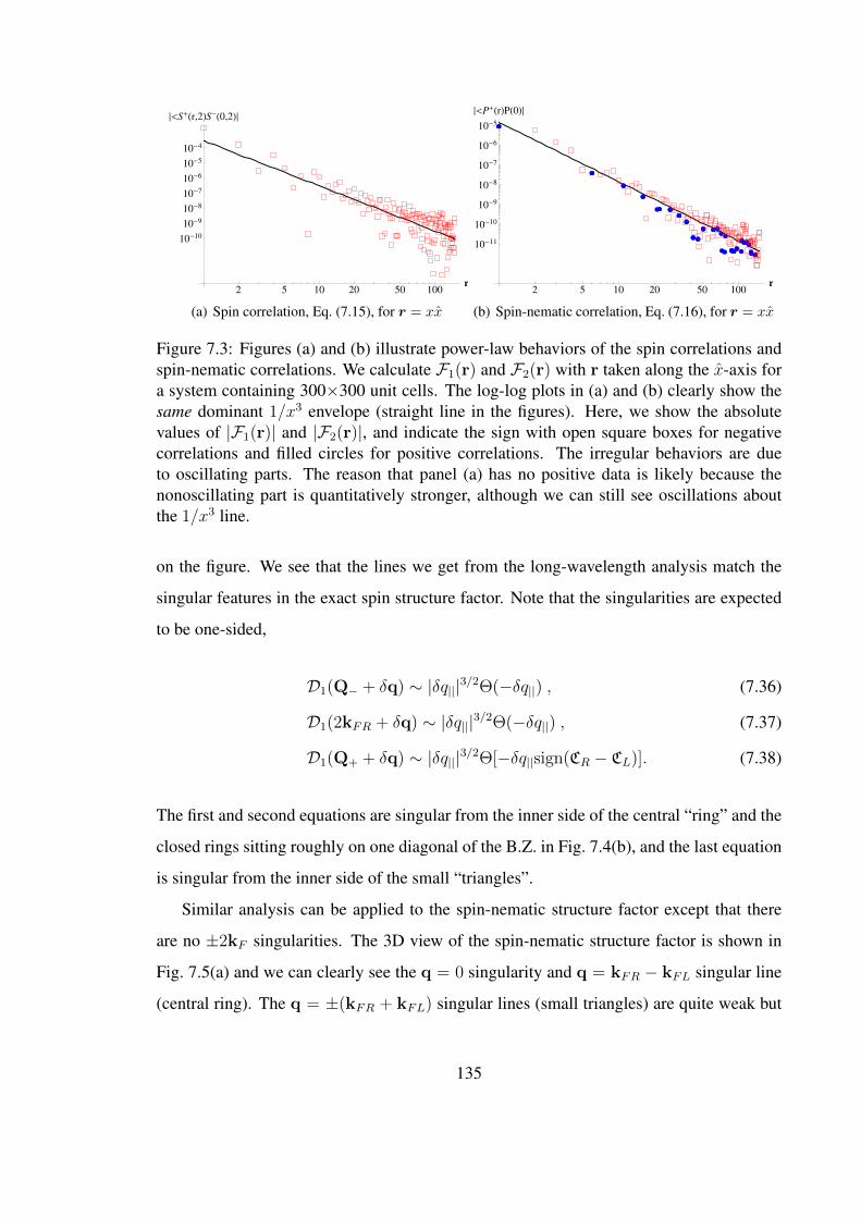
2 5 10 20 50 100r

10-10

10-9

10-8

10-7

10-6

10-5

10-4

È<S+Hr,2LS-H0,2LÈ

(a) Spin correlation, Eq. (7.15), for r = xx

2 5 10 20 50 100r

10-11

10-10

10-9

10-8

10-7

10-6

10-5

È<P+HrLPH0LÈ

(b) Spin-nematic correlation, Eq. (7.16), for r = xx

Figure 7.3: Figures (a) and (b) illustrate power-law behaviors of the spin correlations andspin-nematic correlations. We calculate F1(r) and F2(r) with r taken along the x-axis fora system containing 300×300 unit cells. The log-log plots in (a) and (b) clearly show thesame dominant 1/x3 envelope (straight line in the figures). Here, we show the absolutevalues of |F1(r)| and |F2(r)|, and indicate the sign with open square boxes for negativecorrelations and filled circles for positive correlations. The irregular behaviors are dueto oscillating parts. The reason that panel (a) has no positive data is likely because thenonoscillating part is quantitatively stronger, although we can still see oscillations aboutthe 1/x3 line.

on the figure. We see that the lines we get from the long-wavelength analysis match the

singular features in the exact spin structure factor. Note that the singularities are expected

to be one-sided,

D1(Q− + δq) ∼ |δq|||3/2Θ(−δq||) , (7.36)

D1(2kFR + δq) ∼ |δq|||3/2Θ(−δq||) , (7.37)

D1(Q+ + δq) ∼ |δq|||3/2Θ[−δq||sign(CR − CL)]. (7.38)

The first and second equations are singular from the inner side of the central “ring” and the

closed rings sitting roughly on one diagonal of the B.Z. in Fig. 7.4(b), and the last equation

is singular from the inner side of the small “triangles”.

Similar analysis can be applied to the spin-nematic structure factor except that there

are no ±2kF singularities. The 3D view of the spin-nematic structure factor is shown in

Fig. 7.5(a) and we can clearly see the q = 0 singularity and q = kFR − kFL singular line

(central ring). The q = ±(kFR + kFL) singular lines (small triangles) are quite weak but

135

(a) Three-dimensional view of the spin structure factor (b) Top view of the spin structure factor

Figure 7.4: (a) 3D view of the spin structure factor, D1(q), defined in Eq. (7.20). Wecan clearly see the singularity D1(q) ∼ |q| at q = 0 and we also see weak singularlines: forming central closed ring, two closed rings sitting roughly on one diagonal of theB.Z.; and additional weak singular features near the centers of the latter rings. (b) Thesesingular lines are brought out more clearly when the structure factor is viewed from top. Wesuperposed the locations of the singularities calculated using the Fermi surface information:The inner blue ring specifies the line at kFR − kFL; the red closed rings specify the linesat ±2kF ; the small green triangles specify the lines at ±(kFR + kFL).

still visible, and their locations can be seen more clearly in the view from top shown in

Fig. 7.5(b).

7.3 Majorana spin liquid in the Zeeman field

In the presence of the Zeeman magnetic field, we need to consider the additional term in

the Hamiltonian

HZ = −Bz

∑i

σzi = Bz

∑r,a

icx(r, a)cy(r, a), (7.39)

where we used explicitly the rewriting of spin in terms of Majoranas, Eq. (7.6). We remark

that the Zeeman magnetic field only couples to the spin degrees of freedom (cα Majo-

ranas) and not to the orbital degrees of freedom (dα Majoranas that produce the Z2 gauge

fields). Therefore, the model is exactly solvable even in the presence of the magnetic field.

136

(a) Three-dimensional view of the spin-nematic structurefactor

(b) Top view of the spin-nematic structurefactor

Figure 7.5: (a) 3D view of the spin-nematic structure factor, D2(q), defined in Eq. (7.20).Like the spin structure factor, there is a clear singularity D2(q) ∼ |q| at q = 0 and thereare weak singular lines, one forming a central closed ring and the other forming smalltriangles sitting roughly on one diagonal of the B.Z. (b) The view from the top shows moreclearly the location of the singular lines. We superposed the locations of the singularitiescalculated using the Fermi surface information: The inner blue ring specifies the line atkFR − kFL, and the small green triangles specify the lines at ±(kFR + kFL). Note that,unlike the spin structure factor, there are no ±2kF singularities.

Throughout, we assume the Kp terms, Eq. (7.1), are large enough so that the ground state

remains in the zero Z2 flux sector.

It is interesting to note that the Zeeman term only affects the cx and cy Majoranas while

leaving the cz Majorana unaltered [147, 128]. We can diagonalize the Hamiltonian by

starting with the zero-field solution, Eqs. (7.13)–(7.14). We define two complex fermion

fields,

f †b,+/−(k) ≡ [fx†b (k)± if y†b (k)]/√

2 . (7.40)

137

The Hamiltonian in the Zeeman magnetic field becomes

H =2∑b=1

∑k∈B.Z.

(2εb(k) + 2Bz)

[f †b,−(k)fb,−(k)− 1

2

](7.41)

+2∑b=1

∑k∈B.Z.

(2εb(k)− 2Bz)

[f †b,+(k)fb,+(k)− 1

2

](7.42)

+2∑b=1

∑k∈B.Z.

2εb(k)

[f z†b (k)f zb (k)− 1

2

]. (7.43)

This form implies that f †b,+ carries Sz quantum number +1 and f †b,− carries Sz = −1, while

f z† carries Sz = 0.

An interesting property in this model is that the f z Fermi surface (associated with the

cz Majorana) remains no matter how large the magnetic field is; [128] therefore, there are

always gapless excitations in this system.

For an illustration of several different phases that can occur under the magnetic field,

we take the same parameters as in Fig. 7.2 and examine the effective Zeeman shifting of the

band-1 and band-2 for each complex fermion species. Figure 7.6 shows the magnetization

as a function of magnetic fieldBz. There are quite rich features in this model. When we turn

on the magnetic field, the fb,+ bands move downwards while the fb,− bands move upwards.

First, the field increases up to a threshold value, roughly Bz = 0.024, where the Fermi

surface of the f2,− vanishes and there is a discontinuity in the slope of the magnetization

curve shown in the inset in Fig. 7.6. The f2,+ band is pushed down and the f2,+ Fermi

sea keeps growing until it completely covers the B.Z. at Bz ' 0.5. For the field between

0.5 and 2.8, the f1,+ band remains above the zero energy, and we have the half-polarized

magnetization plateau phase. The f1,+ band reaches zero energy at Bz ' 2.8, we leave

the first plateau phase and the magnetization starts to increase. When the magnetic field

is large enough to completely push the f1,+ band below zero, Bz ' 3.3, the f1,+ Fermi

surface also vanishes and we enter the fully-polarized phase, the second plateau phase. We

also see some weak features in the regimes of increasing magnetization that are due to the

van Hove singularities when the energy passes the saddle points of bands 1 or 2(

see the

contour plot of band 2 in Fig. 7.2(b)), but these van Hove singularities are rather weak in

138

0.02 0.04 0.06Bz

0.01

0.02

0.03

0.04

M z

0.5 1 1.5 2 2.5 3 3.5 4Bz

0.2

0.4

0.5

0.6

0.8

1

M z

Figure 7.6: The magnetization per site, M z ≡ 〈∑

j σzj 〉/Nsites, can be calculated as (ρ1,+ +

ρ2,+ − ρ1,− − ρ2,−)/2, where ρb,± is the population of the fb,± fermions per unit cell.The magnetization curve for our model in the Zeeman field shows rich features (see text)including half- and fully polarized plateaus. The inset shows a blow-up of the small Bz

region where the Fermi surface f2,− disappears and there is a slope discontinuity. We notethat the magnetization inside the unit cell is not completely uniform (because of the reducedlattice symmetries) but is quantitatively similar at each site.

2D.

We remark that in all regimes, the Fermi surface of the f z2 remains the same and gives

gapless excitations. The fully polarized phase is actually the original Kitaev-type model

proposed by Baskaran et al.. [140] This can be seen either directly by examining the phys-

ical Hamiltonian Eq. (7.1), or in the Majorana representation where σzj = 1 = −icxj cyj , so

the constraint becomes Dj = −icxj cyj czjdxj d

yjdzj = czjd

xj d

yjdzj = 1, and the model in terms of

the orbital degrees of freedom reduces to that in [140].

It is interesting that in the half-polarized plateau phase, even though the spin excitations

are gapped, the spin degrees of freedom are entangled in the ground state. The spinless

gapless excitations can be in principle detected by measuring bond-energy correlations or

by entanglement entropy calculations. Finally, the regimes of increasing magnetization

can be viewed as generic compressible Bose-metals [150] in the model with global U(1)

symmetry.

139

7.4 Discussion

We proposed SU(2)-invariant Kitaev-type model on the decorated square lattice that re-

alizes quantum spin liquids with parton Fermi surfaces. Having the benefit of the exact

solutions, we can make robust general observations about such SU(2)-invariant MSL. One

of the distinguishing characteristics of this state is that it has strong spin and spin-nematic

fluctuations as manifested by the same power-law behavior in the correlations considered

in our work. Because of the finite density of states at the Fermi surface, properties such

as the specific heat, spin susceptibility, and NMR relaxation rates are essentially similar to

a metal. Note that the volume/shape of the Fermi sea can be arbitrary, and we can easily

tune the model to have larger or smaller Fermi pockets. In this way, the phase is quite

distinct from the conventional spinon Fermi sea quantum spin liquids, [3] where half of the

Brilloin zone is populated by spin-1/2 spinons before the Gutzwiller projection. Given the

variability of the Fermi surface, the properties of the SU(2) MSL can be very sensitive to

parameters, which we can also easily tune to produce gapped phases.

Let us briefly discuss stability of the exactly solvable model to general perturbations.

First, we note that our complex fermions fα are not conserved microscopically. In principle,

allowed four-fermion interactions would contain terms such as f †αf†βf†γf†δ and f †αf

†βf†γfδ, in

addition to the more familiar terms f †αf†βfγfδ. The origin of the non-conservation of the

complex fermions is because the microscopic fields are Majorana fermions, while we used

the complex fermions as a convenient tool to reduce the problem to more familiar calcula-

tions. However, if the symmetries of the model are sufficiently low, there can be an “emer-

gent” conservation of f -s. For example, if in our treatment we have a very small Fermi

pocket of f -s centered at some momentum K = (Kx, Ky), then the four-fermion terms

f †f †f †f † carry approximate momentum 4K while f †f †f †f carry≈2K, so these terms are

not allowed by momentum conservation if K is some generic non-special wavevector. In

this case, only the familiar terms f †f †ff conserving the fermion number are left and we

have the emergent fermion number conservation law in the long-wavelength theory. The

above is also true in this chapter in which the nonsymmetric small Fermi pockets are real-

ized. Furthermore, only benign forward-scattering four-fermion terms survive in our model

140

since the Cooper-pair interactions carry nonzero momentum. We do not need to consider

six- and eight-fermion terms as they are irrelevant in the renormalization group (RG) sense.

We have chosen a model that lacks time-reversal and lattice point group symmetries so

as not to worry about possible residual pairing instabilities away from the exactly solvable

limit. Such instabilities can be relatively weak also in more symmetric models and the

discussed phenomenology can apply in these cases as well. In Chapter 8 we explore the

stability and the nearby phases by studying such models on ladders [155] using weak-

coupling RG technique and Bosonization analysis [49, 71, 156, 50].

In the presence of the Zeeman magnetic field, there are more interesting phases with

distinct stable Fermi pockets of fb,+, fb,−, and f zb . The Zeeman field breaks the global

SU(2) down to U(1), and the compressible phases in the field are Bose-metal-like phases

[150, 29].

We also found an interesting plateau phase at half-magnetization. Due to the gap for

spin excitations, it is a spin insulator, but since the f z remains gapless, we expect to still

have metal-like specific heat and thermal conductivity.

This behavior in the plateau phase arises because some of the parton constitutents of the

spin operator acquire a gap (band gap in the present case). Some such physics perhaps can

be relevant for the explanation of very recent NMR experiments [22] in EtMe3Sb[Pd(dmit)2]2

showing a drastic reduction in the spin relaxation below temperature of the order 1K as if

a spin gap opens up, while the thermal conductivity measurements and thermodynamic

measurements [23, 25] are consistent with the presence of a Fermi surface of fermionic ex-

citations down to the lowest temperatures. This phenomenology is also qualitatively similar

to Chapter 4 [32] working in a setting closer to the EtMe3Sb[Pd(dmit)2]2 experiments. We

considered a scenario in which, upon writing the spin operator as S+ = f+↑ f↓, there could

be a phase in which one spinon species becomes gapped due to pairing, while the other

species retains the Fermi surface. It is fascinating to further explore such idea where some

partons are gapped and some are gapless in more realistic settings.

141

Chapter 8

Majorana spin liquids on a two-legladder

In Chapter 7 we constructed an exactly solvable microscopic model in Kitaev’s spirit to

study the properties of such SU(2)-invariant Majorana spin liquids (MSL) with Fermi sur-

faces of partons [157]. However, we allowed very low symmetries—lack of parity, in-

version, and time reversal symmetry (TRS)—to sidestep discussing possible perturbations

such as Cooper pairing instability, which can destabilize the gapless quantum spin liquids

(QSL) phases away from the exactly solvable limit. In order to study the stability of such

new class of gapless QSL and further explore their properties, we realize such states on a

two-leg square ladder and show that they represent new quasi-1D phases.

We first consider a gapless Majorana orbital liquid (MOL) realized in a Kitaev-type

model on the two-leg ladder using orbital degrees of freedom. The system can be reduced

to one species of Majorana fermions coupled to background Z2 gauge fields such that it

is exactly solvable and has gapless partons with incommensurate Fermi wave vectors. We

formulate a long-wavelength description in terms of right-moving and left-moving com-

plex fermions fR/L and show that local energy observable has power law correlations at

incommensurate “2kF ” wavevectors. Going away from the exactly solvable point, we first

consider allowed residual parton interactions and find that there is only one valid four-

fermion term and it is strictly marginal; hence, the MOL is stable to such perturbations.

An important question is the stability of the MOL to allowing Z2 gauge field fluctua-

tions, as these lead to confinement of partons in gapped phases in so-called even Z2 gauge

142

theories in (1+1)D [11, 158]. We argue that because of the nontrivial momenta carried by

the gapless partons, there is a destructive interference for Z2 vortices (instantons) in space-

time, and hence these are suppressed and do not affect the count of gapless modes. The

local energy observables obtain new contributions beyond the mean field, and in this sense

the partons become “less free”, but their bosonized fields still remain very convenient for

characterizing the MOL phase.

We next realize an SU(2)-invariant MSL using both spin-1/2 and orbital degrees of

freedom [149, 147] at each site of the two-leg ladder [130]. The system can be reduced to

three species of Majorana fermions coupled to background Z2 gauge fields such that it is

exactly solvable and has gapless partons with incommensurate wave vectors. We formu-

late long-wavelength description in terms of three right-moving and left-moving complex

fermions (fxR/L, fyR/L, f

zR/L) that transform as a vector under spin rotation. Because there

is no global U(1) symmetry, in addition to familiar four-fermion residual interactions ex-

pressed as fα†R fβ†L fγRf

δL, there are other allowed terms such as fα†R fβ†L f

γ†R f

δ†L . Despite of

having more allowed interactions, a weak coupling renormalization group (RG) analysis

gives a large regime of a stable phase. Similarly to the MOL case, we argue that such MSL

with gapless matter can be also stable against Z2 gauge field fluctuations even in (1+1)D

[159, 160, 158].

The chapter is organized as follows. In Chapter 8.1, we realize the MOL with one

fermion species in a Kitaev-type model [14] on the two-leg ladder and consider its long-

wavelength properties and stability against perturbations. In Chapter 8.2, we realize the

SU(2) MSL and use weak coupling RG analysis to study the stability of such phase against

residual parton interactions and also discuss the stability against gauge field fluctuations.

We conclude in Chapter 8.3 with some discussions. In Appendix 8.A, we consider more

abstractly the stability of gapless U(1) matter against Z2 gauge field fluctuations in (1+1)D.

In Appendix 8.B, we give long-wavelength description of the SU(2) MSL and discuss ob-

servable properties. In Appendix 8.C, we consider Zeeman magnetic fields on the SU(2)

MSL. In Appendix 8.D, we realize the SU(2) MSL in a model with explicitly broken time

reversal symmetry and show that this case has a larger window of stability to weak pertur-

bations.

143

8.1 Gapless Majorana orbital liquid (MOL) on a two-leg

ladder

We begin with a “spinless” (one species) MOL realized in a Kitaev-type model on a two-leg

ladder shown in Fig. 8.1(a). The Hamiltonian is

H = H0 +K�xz∑�xz

W�xz +K�yz∑�yz

W�yz , (8.1)

where

H0 =∑

λ−link,〈jk〉

Jjkτλj τ

λk , (8.2)

W�xz = τ y1 τy2 τ

y3 τ

y4 , (8.3)

W�yz = τx2 τx1 τ

x4 τ

x3 . (8.4)

The ~τ Pauli matrices can be thought of as acting on two-level orbital states. The Wp terms,

with p = �xz or �yz formed by x and z or y and z links, respectively, are plaquette oper-

ators which commute among themselves and with all other terms in the Hamiltonian and

are added to stabilize particular flux sector, see Fig. 8.1(a). Following Kitaev’s approach,

we introduce Majorana representation as

ταj = ibαj cj, (8.5)

with the constraint Dj ≡ bxj byj bzjcj = 1. The Hamiltonian can be rephrased as

H0 = i∑〈jk〉

ujkJjkcjck , (8.6)

Wp={�xz ,�yz} = −∏〈jk〉∈p

ujk , (8.7)

where ujk ≡ −ibλj bλk for λ-link 〈jk〉 and the product in the last line is circling the plaquette.

Following familiar analysis in Kitaev-type models, we observe that in the enlarged

144

x

x

z

1 2

34 y

y

y

y

x

x

z

1 2

34

unit cell

y

y

(a)

Band-1

Band-2

RL-Π -Π

2

Π

2Π

k

-1

1

2

3

Εk

(b)

Figure 8.1: (a) Graphical representation of the exactly solvable Kitaev-type model on thetwo-leg ladder and its solution in the zero flux sector. The c Majoranas propagate with pureimaginary hopping amplitudes specified by the couplings Jx, Jy, Jz, and J ′z; the signsin our chosen gauge are indicated by the arrows and the four-site unit cell is also indi-cated. (b) Dispersion of complex fermions that solve the Majorana problem for parameters{Jx, Jy, Jz, J ′z} = {1.2, 0.8, 1.0, 1.1}

Hilbert space, ujk commute among themselves and with the Hamiltonian, and we can pro-

ceed by replacing them by their eigenvalues ±1 and interpreting as static Z2 gauge fields.

The Wp terms, with Kp > 0 assumed to be sufficiently large, can be used to stabilize the

sector with zero fluxes through all elementary plackets, and this can give a gapless phase.

In our work, we fix the gauge by taking ujk = 1 for bonds j → k as shown by the arrows

in Fig. 8.1(a).

There are four physical sites per unit cell, so there are four Majoranas per unit cell.

From now on, we replace the site labeling j with j = {X, a}, where X runs over the one-

dimensional lattice of unit cells of the ladder and a runs over the four sites in the unit cell,

see Fig. 8.1(a). The Hamiltonian can be written as,

H =∑〈jk〉

cjAjkck =∑

〈(X,a),(X′,a′)〉

cX,aAX,a;X′,a′cX′,a′ .

There is translational symmetry between different unit cells, and AX,a;X′,a′ = Aaa′(X −

X ′).

In order to give a concise long-wavelength description, it will be convenient to use

familiar complex fermion fields. To this end, we can proceed as follows. For a general

145

Majorana problem specified by an anti-symmetric pure imaginary matrix Ajk, we diago-

nalize Ajk for spectra, but only half of the bands are needed while the rest of the bands

can be obtained by a specific relation and are redundant. Explicitly, for a system with

2m bands, we can divide them into two groups. The first group contains bands from 1

to m with eigenvector-eigenenergy pairs {~vb,k, εb,k}, where b = 1, 2, . . . ,m are band in-

dices, and the second group contains bands from m + 1 to 2m related to the first group,

{~vb′=m+b,k, εb′=m+b,k} = {~v∗b,−k,−εb,−k}. Using only the bands with b = 1 to m, we can

write the original Majoranas in terms of usual complex fermions as

c(X, a) =

√2

Nuc

m∑b=1

∑k∈B.Z.

[eikXvb,k(a)fb(k) + H.c.

],

where Nuc is the number of unit cells, B.Z. stands for the Brillouin zone, and the complex

fermion field f satisfies the usual anticommutation relation, {f †b (k), fb′(k′)} = δbb′δkk′ . In

terms of the complex fermion fields, the Hamiltonian becomes

H =m∑b=1

∑k∈B.Z.

2εb(k)

[f †b (k)fb(k)− 1

2

]. (8.8)

In the present case, 2m = 4 and therefore two bands are sufficient to give us the full

solution of the Majorana problem.

The above approach can be applied to any general Majorana problem and is needed

when we consider a model lacking any symmetries in Appendix 8.D. In the present case,

we require the model to respect time reversal symmetry [14] and leg interchange symmetry,

which allows us to introduce convenient complex fermion fields already on the lattice scale

as follows

fI(X) =c(X, 1) + ic(X, 4)

2, (8.9)

fII(X) =−ic(X, 2) + c(X, 3)

2. (8.10)

146

The Hamiltonian becomes

H = 2∑X

{Jzf

†I (X)fI(X) + J ′zf

†II(X)fII(X)−

−[Jxf

†I (X)fII(X) + Jyf

†II(X)fI(X + 1) + H.c.

]},

where we ignored constant contribution. It is easy to calculate the band dispersions,

ε(k) = J+z ±

√(J−z )2 + J2

x + J2y + 2JxJy cos(k), (8.11)

with J±z = (Jz ± J ′z)/2. The spectrum is gapless for |Jx− Jy| ≤√JzJ ′z ≤ Jx + Jy, where

without loss of generality we assumed all couplings to be positive. For an illustration of

the energy spectrum, we take {Jx, Jy, Jz, J ′z} = {1.2, 0.8, 1.0, 1.1} and show the two

bands of the complex fermions in Fig. 8.1(b) labeled from top to bottom as band-1 and

band-2. We note that the gapless phase occur in a large parameter regime and there is no

fine tuning here. The specific parameters are chosen to emphasize that we do not require

any symmetries other than time reversal and leg interchange.

The band-2 crosses zero at kFR and kFL = −kFR from time reversal. For long wave-

length physics, we can focus on this band and introduce continuum complex fermion fields

fR/L; for the lattice Majoranas, we obtain the expansion,

c(X, a) ∼∑

P=R/L

[eikFPXv2,P (a)fP (X) + H.c.

]. (8.12)

From the detailed band calculation, at the right Fermi point

~v2,R =

√J ′z

4J+z

1

iξ

ξ

−i

, (8.13)

where ξ = (Jx + JyeikFR)/J ′z. Using time reversal invariance, for the left Fermi point we

147

get v2,L(a) = (−1)a+1v∗2,R(a). The effective low-energy Hamiltonian density is

H = vF

[f †R(−i∂x)fR − f †L(−i∂x)fL

], (8.14)

describing a one-dimensional Dirac particle with Fermi velocity vF = JxJy sin(kFR)/J+z .

We list the symmetry transformations of the continuum fields in Table 8.1 (ignoring the

“spin” indices there). In particular, the leg interchange symmetry prohibits terms of the

form fRfL from the continnum Hamiltonian that would gap out the spectrum.

8.1.1 Fixed-point theory of Majorana orbital liquid and observables

In this subsection, we first give the fixed-point theory of the MOL and then we will con-

sider bond energy operators to characterize such gapless phase. We use bosonization, re-

expressing the low-energy fermion operators with bosonic fields [156, 71, 106],

fP = ei(ϕ+Pθ) , (8.15)

with canonical conjugate boson fields:

[ϕ(x), ϕ(x′)] = [θ(x), θ(x′)] = 0 , (8.16)

[ϕ(x), θ(x′)] = iπΘ(x− x′) , (8.17)

where Θ(x) is the heaviside step function.

The fixed-point bosonized Lagrangian of such gapless MOL is

LMOL =1

2πg

[1

v(∂τθ)

2 + v(∂xθ)2

]. (8.18)

For free fermions, g = 1 and v = vF , the bare Fermi velocity. Later when we discuss

the stability of such a phase in Chapter 8.1.2, we will see that there is only one strictly

marginal interaction which introduces one Luttinger parameter g. To detect the gaplessness

of the phase using physical (gauge-invariant) observables, here we consider bond-energy

operators [63], Bs/a(X), which we further categorize into symmetric or antisymmetric with

148

respect to the leg interchange symmetry. The specific microscopic operators are

Bs/a(X) = τx(X, 1)τx(X, 2)± τx(X, 4)τx(X, 3)

= iu12c(X, 1)c(X, 2)± iu43c(X, 4)c(X, 3), (8.19)

where we used Majorana representation, Eq. (8.5). In our gauge, after expansion in terms

of the continuum complex fermions using Eq. (8.12), the Fourier components are organized

as follows

BsQ=0 ∼ f †RfR + f †LfL =∂xθ

π, (8.20)

BskFR−kFL ∼ f †LfR = iei2θ, (8.21)

BakFR+kFL∼ fLfR = −iei2ϕ. (8.22)

(Note that with TRS, the wave vector kFR + kFL is the same as Q = 0; to be more

precise, we should write a Hermitian and time reversal symmetric combination, BaQ=0 =

ifLfR+H.c.)

Thus, the symmetric bond-energy correlations are expected to decay with os-

cillations at incommensurate wave vectors ±2kFR, while the anti-symmetric bond-energy

correlations decay without oscillations. Such a sharp difference can be confirmed in exact

numerical calculations.

In the bosonized form, the scaling dimension of each term is apparent,

∆[BsQ=0] = 1, (8.23)

∆[Bs2kFR ] = g, (8.24)

∆[BaQ=0] =1

g. (8.25)

In the non-interacting parton limit, g → 1, we expect to see all components of bond-energy

correlations decay as X−2.

For illustration, we calculate correlations in the exactly solvable model, taking the same

parameters as in Fig. 8.1. Figure 8.2(a) shows log-log plot of symmetric bond-energy cor-

relations in a finite system with 500 unit cells, while Figure 8.2(b) shows antisymmetric

149

2 5 10 20 50 100 200X

10-6

10-5

10-4

0.001

0.01

È<BsH0LBsHXL>È

(a) Leg-symmetric energy correlation

2 5 10 20 50 100 200X

10-5

10-4

0.001

0.01

È<BaH0LBaHXL>È

(b) Leg-antisymmetric energy correlation

Figure 8.2: Figures (a) and (b) illustrate power law behaviors of the symmetric and anti-symmetric bond energy correlations, withBs/a defined in Eq. (8.19), in the exactly solvablemodel with noninteracting partons. The system has 500 unit cells and we use the sameparameters as in Fig. 8.1. We plot absolute values and indicate the sign with filled circles(blue) for positive correlations and open square boxes (red) for negative correlations. Thelog-log plots clearly show X−2 decay (straight lines) with incommensurate oscillationsin the symmetric case and no oscillations in the antisymmetric case. The characteristicwavevectors can be determined from the structure factor study shown in Fig. 8.3.

bond-energy correlations [161]. We can see the overall X−2 envelope in both figures and

also incommensurate oscillations in the symmetric bond-energy correlations, which con-

firm the theoretical analysis above.

Power-law correlations in real space correspond to singularities in momentum space,

which we can study by considering the corresponding structure factors. Figure 8.3(a) shows

the symmetric bond-energy structure factor and Fig. 8.3(b) shows the anti-symmetric bond-

energy structure factor. It is clear that the singularities in the symmetric case occur exactly

at Q = 0 and Q = ±(kFR − kFL) = ±2kFR ≡ ±2kF (which we also mark using values

obtained by extracting the Fermi points of band 2), while there is only Q = 0 singularity

for the anti-symmetric case.

Let us now consider some other operators similar to generic XYZ energy terms but not

present in the exactly solvable model; this will be also useful for the subsequent discussion

of the MOL stability. First, operators like τ y(X, 1)τ y(X, 2) and τ z(X, 1)τ z(X, 2) have

ultra-short-ranged correlations as they contain unpaired localized b-fermions. It is more

interesting to consider operators like τx(X, 1)τx(X, 4) defined on the z-type (vertical) links

in Fig. 8.1. In this case, even though the local operator contains unpaired b-Majoranas, in

the physical Hilbert space these can actually be paired at the expense of introducing a string

150

2 kF-2 Π -2 kF +2 Π

-Π -Π

2

Π

2Π

q

0.6

0.8

1.0

1.2

1.4

(a) Leg-symmetric energy structure factor

-Π -Π

2

Π

2Π

q

1.4

1.5

1.6

1.7

1.8

(b) Leg-antisymmetric energy structure factor

Figure 8.3: Figures (a) and (b) illustrate the symmetric bond-energy and antisymmetricbond-energy structure factors corresponding to Figs. 8.2(a) and 8.2(b), respectively. Bothcases clearly show a singularity atQ = 0, while the symmetric case also shows singularitiesat ±2kF .

product of the gapless c-Majoranas. For example, consider calculating correlation between

rungs at X and X ′:

F(X,X ′) ≡ τx(X, 1)τx(X, 4) τx(X ′, 1)τx(X ′, 4) =

=∏

X≤X′′<X′(−1)c(X ′′, 1)c(X ′′, 4)c(X ′′, 2)c(X ′′, 3)×

×∏

〈(X,1),(X,4)〉 < λ−link 〈ij〉 ≤ 〈(X′,1),(X′,4)〉

uλij (8.26)

where the last product contains all links on the ladder located between the two vertical

links excluding 〈(X, 1), (X, 4)〉 and including 〈(X ′, 1), (X ′, 4)〉 and oriented as shown in

Fig. 8.1. The second line is 1 in our chosen gauge, and we then have a factor of

(−1)c(X ′′, 1)c(X ′′, 4)c(X ′′, 2)c(X ′′, 3) = eiπ[f†I (X′′)fI(X′′)+f†II(X

′′)fII(X′′)] (8.27)

for each unit cell, where we used Eqs. (8.9)–(8.10). In the present gauge, we can write

schematically τx(X, 1)τx(X, 4) ∼∏

X′′<X(−1)c(X ′′, 1)c(X ′′, 4)c(X ′′, 2)c(X ′′, 3), and see

that this contains non-local Jordan-Wigner-like string operator in terms of the gapless par-

151

2 5 10 20 50X

0.10

0.20

0.30

0.15

ÈFHXLÈ

Figure 8.4: Figure illustrates power-law behavior of the correlation F(X − X ′) =〈F(X,X ′)〉, defined in Eq. (8.26). The system has 100 unit cells in chain length andthe same parameters as in Fig. 8.1. We show the absolute values of |F(X)| and indicatethe sign with filled circles (blue) for positive correlations and open square boxes (red) fornegative correlations. The log-log plot clearly shows X−1/2 envelope (straight line in thefigure). The irregular behavior is due to incommensurate oscillations.

tons. In the bosonization language, the string operator becomes

∏X′′<X

eiπ[f†I (X′′)fI(X′′)+f†II(X

′′)fII(X′′)] ∼ e±i[θ(X)+πnX]. (8.28)

This has scaling dimension 1/4 in the free-fermion case and hence the above correlation

decays as X−1/2 power law and oscillates at wavevector πn = kF from Fig. 8.1(b). It

may seem unusual that this appears to contain the specific gauge-dependent quantity kF ;

note, however, that in the full calculation we used the specific gauge to set the last line in

Eq. (8.26) to unity, and the final result is independent of the gauge.

Evaluating expectation value of the string operator in the free fermion ground state leads

to a Pfaffian of a matrix formed by the Majorana contractions and can be easily computed

numerically for reasonable sizes [162]. The results are shown in Fig. 8.4 for a system

with 100-unit cells [161]. The corresponding structure factor is shown in Fig. 8.5. We can

clearly see the singularities at ±kF and confirm our theoretical analysis.

8.1.2 Stability of Majorana orbital liquid

Let us now consider going away from the exactly solvable point. First, we consider pertur-

bations that are local in the continuum fermion fields. This ignores fluctuations in the Z2

152

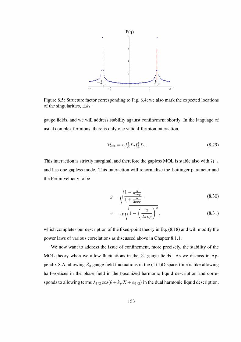
kF

-kF

-Π -Π

2

Π

2Π

q

2

4

6

8

FHqL

Figure 8.5: Structure factor corresponding to Fig. 8.4; we also mark the expected locationsof the singularities, ±kF .

gauge fields, and we will address stability against confinement shortly. In the language of

usual complex fermions, there is only one valid 4-fermion interaction,

Hint = uf †RfRf†LfL . (8.29)

This interaction is strictly marginal, and therefore the gapless MOL is stable also withHint

and has one gapless mode. This interaction will renormalize the Luttinger parameter and

the Fermi velocity to be

g =

√1− u

2πvF

1 + u2πvF

, (8.30)

v = vF

√1−

(u

2πvF

)2

, (8.31)

which completes our description of the fixed-point theory in Eq. (8.18) and will modify the

power laws of various correlations as discussed above in Chapter 8.1.1.

We now want to address the issue of confinement, more precisely, the stability of the

MOL theory when we allow fluctuations in the Z2 gauge fields. As we discuss in Ap-

pendix 8.A, allowing Z2 gauge field fluctuations in the (1+1)D space-time is like allowing

half-vortices in the phase field in the bosonized harmonic liquid description and corre-

sponds to allowing terms λ1/2 cos(θ+kFX+α1/2) in the dual harmonic liquid description,

153

Eq. (8.18). The key point is that this term is oscillating for generic kF and hence averages

out to zero (the underlying physics is destructive interference due to Berry phases). Thus,

our gapless MOL with incommensurate momenta carried by the fermion fields persists also

in the presence of Z2 gauge field dynamics even in (1+1)D, in the sense that we retain the

gapless mode.

One may worry about the precise connection between the present system and the schematic

Z2 gauge theory plus U(1) matter at incommensurate density considered in Appendix 8.A.

Indeed, the connection is only crude, and we do not have one-to-one correspondences.

Nevertheless, we can bolster our argument by considering explicitly some allowed pertur-

bations to the exactly solvable model. Consider, e.g., adding small general XYZ interac-

tions∑〈ij〉∑

µ=x,y,z δJµijτ

µi τ

µj on all bonds in a manner respecting the underlying lattice

symmetries. As we have discussed earlier, δJy,z terms on the x-type bonds and δJx,z terms

on the y-type bonds have short-range correlations and hence constitute irrelevant perturba-

tions (of course, they can renormalize the Luttinger parameter). On the other hand, δJx,y

terms on the z-type bonds have power law correlations. However, these correlations oscil-

late at the incommensurate wavevector, see Fig. 8.4 and Fig. 8.5. Hence such terms, whose

structure is similar to λ1/2 cos(θ + kFX + α1/2), see Eq. (8.28), are washed out from the

low-energy Hamiltonian. Thus, the fixed point description is the same as described ear-

lier, but with the additional remark that now generic energy correlations that are symmetric

under the leg interchange will also obtain a contribution oscillating at wavevector kF with

scaling dimension g/4.

Finally, we remark that the Z2 gauge fluctuations do lead to confinement in our two-leg

model in gapped regimes, e.g., when the Jz terms dominate over the Jx, Jy terms in the

original Hamiltonian Eq. (8.1). In this regime, we can start with effective (super)-spins on

the rungs formed by the large Jz terms (e.g., after conveniently making the Jz coupling

ferromagnetic). We perturbatively derive effective Hamiltonian governing these effective

spins, which works out to be an Ising-like chain and has two degenerate ground states.

Adding the δJx,y perturbations on the z-type bonds gives local longitudinal fields in this

Ising chain and immediately lifts the degeneracy. Hence, there is a unique ground state.

Furthermore, creating a single domain-wall-like excitation, which behaves as a free

154

particle in the exactly solvable model, requires infinite energy in the presence of the longi-

tudinal field. On the other hand, a pair of domain walls, kink and anti-kink, are allowed, but

to separate one from the other requires energy linearly proportional to the distance between

them. Therefore, such δJx,y perturbations on the z-type bonds give linear confinement of

particles that were free at the exactly solvable point, and this applies to all particles that

carry gauge charge with respect to the Z2 gauge field in the exactly solvable model.

8.2 Gapless SU(2)-invariant Majorana spin liquid (MSL)

on the two-leg ladder

We now want to consider Majorana spin liquids with more degrees of freedom, in particular

with physical spin degrees of freedom, and see what new issues and features arise in this

case. In order to construct spin SU(2)-invariant Kitaev-type model, we follow [149, 147,

157] to take a system with both spin and orbital degrees of freedom on each site. The

complete Hamiltonian is

HSU(2) = H′0 +K�xz∑�xz

W�xz +K�yz∑�yz

W�yz , (8.32)

where

H′0 =∑

λ−link,〈jk〉

Jjk(τλj τ

λk

)(~σj · ~σk) . (8.33)

H′0 is a Kugel-Khomskii-like Hamiltonian with ~σ being the spin-1/2 Pauli matrices and ~τ

being the Pauli matrices acting on the orbital states, while the W�xz and W�yz terms are

given in Eqs. (8.3)–(8.4).

Introducing Majorana representation of spin-1/2, we write the spin and orbital operators

155

as

σαj = − i2

∑β,γ

εαβγcβj cγj , (8.34)

ταj = − i2

∑β,γ

εαβγdβj dγj . (8.35)

On each site j of the two-leg ladder, we realize the physical four-dimensional Hilbert

space using six Majorana fermions cxj , cyj , czj , d

xj , dyj , and dzj , with the constraint Dj ≡

−icxj cyj czjdxj d

yjdzj = 1 (namely, for any physical state |Φ〉phys, we require Dj|Φ〉phys =

|Φ〉phys). Therefore, σαj τβj |Φ〉phys = icαj d

βj |Φ〉phys. In terms of the Majoranas, the Hamilto-

nian can be rephrased as

H′0 = i∑〈jk〉

ujkJjk∑

α=x,y,z

cαj cαk , (8.36)

and the Wp terms are the same as in Eq. (8.7) with ujk ≡ −idλj dλk for λ-link 〈jk〉.

For long-wavelength description, much of the development in Chapter 8.1 can be di-

rectly applied here with the replacement, c→ cα, f → fα, α = x, y, z. We now have three

fermion species with identical dispersion taken to be similar to that in Fig. 8.1(b), and we

introduce right and left moving complex fermion fields fαR/L as in the spinless case. Under

SU(2) spin rotations, the triple fx,y,z transforms in the same way as the physical spin σx,y,z.

Just as in the MOL case in Chapter 8.1, we first establish the fixed point structure

ignoring the gauge field fluctuations. In order to study the stability of such gapless SU(2)-

invariant Majorana spin liquid under weak perturbations, we write down most general four-

fermion interactions and perform renormalization group (RG) studies. The allowed four-

fermion interactions are highly constrained by symmetry. In addition to the SU(2) spin ro-

tation invariance, these terms must be preserved by projective symmetry group (PSG) [13]

of spatial translational symmetry, time reversal symmetry, and leg interchange symmetry.

We list the symmetry transformations in Table 8.1 and write the allowed nonchiral interac-

156

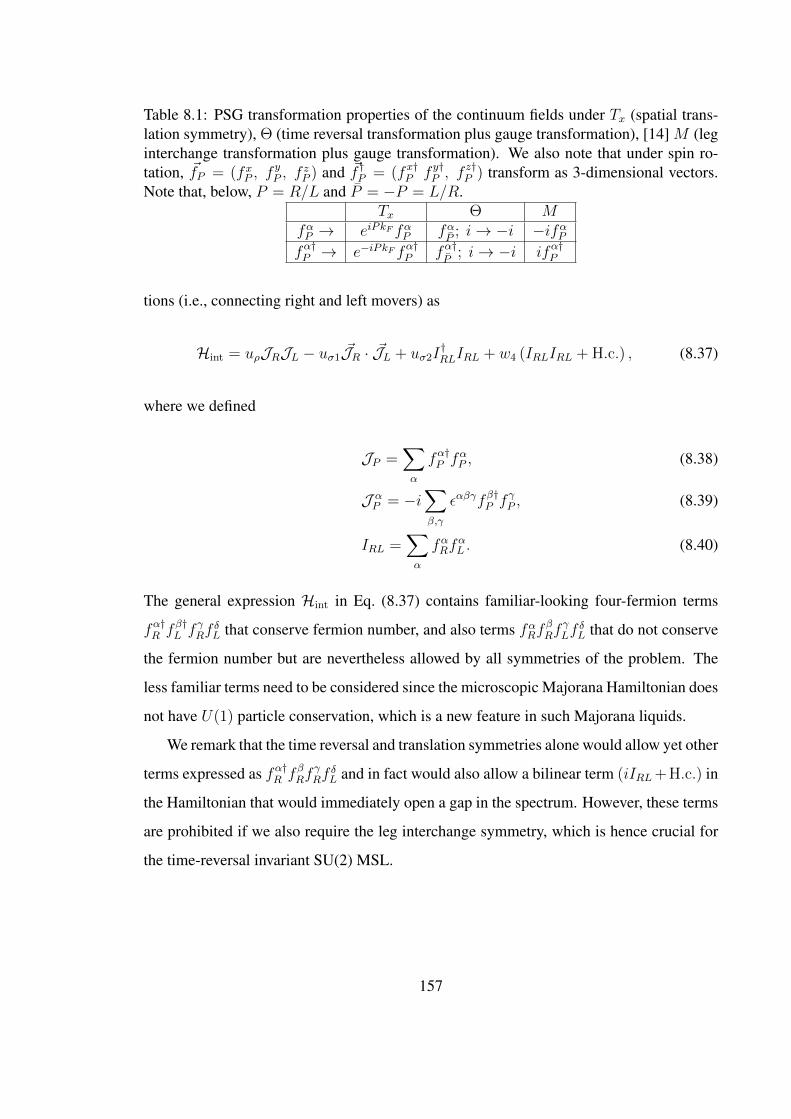
Table 8.1: PSG transformation properties of the continuum fields under Tx (spatial trans-lation symmetry), Θ (time reversal transformation plus gauge transformation), [14] M (leginterchange transformation plus gauge transformation). We also note that under spin ro-tation, ~fP = (fxP , f

yP , f

zP ) and ~f †P = (fx†P f y†P , f

z†P ) transform as 3-dimensional vectors.

Note that, below, P = R/L and P = −P = L/R.Tx Θ M

fαP → eiPkF fαP fαP

; i→ −i −ifαPfα†P → e−iPkF fα†P fα†

P; i→ −i ifα†P

tions (i.e., connecting right and left movers) as

Hint = uρJRJL − uσ1~JR · ~JL + uσ2I

†RLIRL + w4 (IRLIRL + H.c.) , (8.37)

where we defined

JP =∑α

fα†P fαP , (8.38)

J αP = −i

∑β,γ

εαβγfβ†P fγP , (8.39)

IRL =∑α

fαRfαL . (8.40)

The general expression Hint in Eq. (8.37) contains familiar-looking four-fermion terms

fα†R fβ†L fγRf

δL that conserve fermion number, and also terms fαRf

βRf

γLf

δL that do not conserve

the fermion number but are nevertheless allowed by all symmetries of the problem. The

less familiar terms need to be considered since the microscopic Majorana Hamiltonian does

not have U(1) particle conservation, which is a new feature in such Majorana liquids.

We remark that the time reversal and translation symmetries alone would allow yet other

terms expressed as fα†R fβRfγRf

δL and in fact would also allow a bilinear term (iIRL+H.c.) in

the Hamiltonian that would immediately open a gap in the spectrum. However, these terms

are prohibited if we also require the leg interchange symmetry, which is hence crucial for

the time-reversal invariant SU(2) MSL.

157

The weak-coupling differential RG equations are

uρ =1

2πv

(u2σ2 + 2uσ1uσ2 − 4w2

4

), (8.41)

uσ1 =1

2πv

(−u2

σ1 + 2uσ1uσ2

), (8.42)

uσ2 =1

2πv

(−3u2

σ2 − 6uσ1uσ2 − 4w24

), (8.43)

w4 =1

2πv(−2uσ1 − 4uσ2 − 4uρ)w4, (8.44)

where v is the Fermi velocity of right and left movers and O ≡ dO/d` with ` being log-

arithm of the length scale. The only fixed points have u∗σ1 = u∗σ2 = w∗4 = 0. Stability

to small deviations in w4 requires u∗ρ > 0. If we consider small deviations in uσ1 and uσ2

setting w∗4 = 0, the RG equations can be written as

gρ ≡ 3uρ + uσ2 = 0, (8.45)

uσ1 =1

2πv(−u2

σ1 + 2uσ1uσ2), (8.46)

uσ2 =1

2πv(−3u2

σ2 − 6uσ1uσ2), (8.47)

and the last two equations are essentially identical to the RG equations in a level-one SU(3)

Wess-Zumino-Witten (WZW) model discussed by Itoi and Kato. [163] Translated from

their analysis, the stability to small deviation in uσ1 and uσ2 requires uσ1 > 0, uσ1 +uσ2 >

0. In a stable flow, uρ reaches some fixed value, u∗ρ > 0, and is strictly marginal; uσ1 and

uσ2 approach zero from the specific region described above and are marginally irrelevant;

finally, w4 flows to zero as long as u∗ρ > 0 and is irrelevant. Thus, we have one Luttinger

parameter in the “charge” sector. In Appendix 8.B, we give the fixed-point theory of the

SU(2) MSL and list observables that can be obtained as fermion bilinears. We find that

spin operator, Eq. (8.64), spin-nematic operator, Eq. (8.66), and bond-energy operator,

Eq. (8.65), have correlations that decay in a power law with oscillations at incommensurate

wave vectors, which is one of the hallmarks of such Majorana spin liquids as we discussed

in [157] in a 2d example.

The inclusion of the Z2 gauge field fluctuations in this quasi-1d gapless MSL can be

158

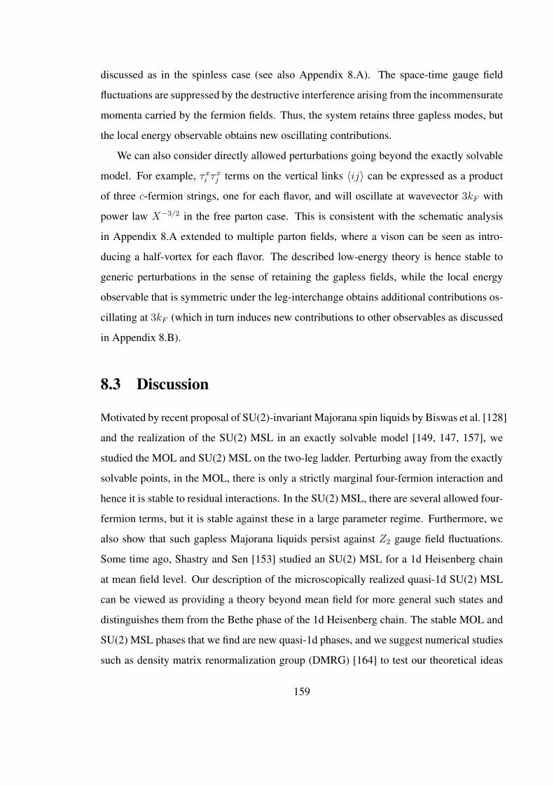
discussed as in the spinless case (see also Appendix 8.A). The space-time gauge field

fluctuations are suppressed by the destructive interference arising from the incommensurate

momenta carried by the fermion fields. Thus, the system retains three gapless modes, but

the local energy observable obtains new oscillating contributions.

We can also consider directly allowed perturbations going beyond the exactly solvable

model. For example, τxi τxj terms on the vertical links 〈ij〉 can be expressed as a product

of three c-fermion strings, one for each flavor, and will oscillate at wavevector 3kF with

power law X−3/2 in the free parton case. This is consistent with the schematic analysis

in Appendix 8.A extended to multiple parton fields, where a vison can be seen as intro-

ducing a half-vortex for each flavor. The described low-energy theory is hence stable to

generic perturbations in the sense of retaining the gapless fields, while the local energy

observable that is symmetric under the leg-interchange obtains additional contributions os-

cillating at 3kF (which in turn induces new contributions to other observables as discussed

in Appendix 8.B).

8.3 Discussion

Motivated by recent proposal of SU(2)-invariant Majorana spin liquids by Biswas et al. [128]

and the realization of the SU(2) MSL in an exactly solvable model [149, 147, 157], we

studied the MOL and SU(2) MSL on the two-leg ladder. Perturbing away from the exactly

solvable points, in the MOL, there is only a strictly marginal four-fermion interaction and

hence it is stable to residual interactions. In the SU(2) MSL, there are several allowed four-

fermion terms, but it is stable against these in a large parameter regime. Furthermore, we

also show that such gapless Majorana liquids persist against Z2 gauge field fluctuations.

Some time ago, Shastry and Sen [153] studied an SU(2) MSL for a 1d Heisenberg chain

at mean field level. Our description of the microscopically realized quasi-1d SU(2) MSL

can be viewed as providing a theory beyond mean field for more general such states and

distinguishes them from the Bethe phase of the 1d Heisenberg chain. The stable MOL and

SU(2) MSL phases that we find are new quasi-1d phases, and we suggest numerical studies

such as density matrix renormalization group (DMRG) [164] to test our theoretical ideas

159

of their stability. The DMRG studies can also determine the Luttinger parameters of the

fixed-point MOL and SU(2) MSL theories.

The presence of gapless matter fields is the key against confining effects of Z2 gauge

field fluctuations in (1+1)D, see Appendix 8.A. Without such gapless matter, the gapped

phases realized in Kitaev-type models on two-leg ladders in our model are likely unstable to

general generic perturbations, and this prediction can be checked by DMRG studies. This

is reminiscent of a picture where gapless matter fields can suppress monopoles in a (2+1)D

compact electrodynamics and thus make gapless U(1) spin liquids with sufficiently many

Dirac points or with Fermi surfaces stable [3, 165, 166], while gapped U(1) spin liquids

would be unstable to confinement in (2+1)D. An interesting finding is that allowing Z2

gauge fluctuations in our quasi-1d Majorana liquids leads to new contributions to various

observables, with different characteristic wavevectors and potentially slower power laws

compared to the mean field, see Appendix 8.B.

Let us discuss possible extensions of this work. Throughout, we focused on the MSL

phase in which all couplings of the residual interactions, Eq. (8.37), converge to finite

fixed point values in RG thinking. In principle, one can analyze situations where some of

the residual interactions are relevant and explore possible nearby phases and characterize

their properties using the observables listed in Appendix 8.B. Such theoretical analysis

combined with DMRG studies [29] can give a complete phase diagram.

As discussed in Biswas et al. [128] and in our earlier work [157], the effects of Zeeman

field on the SU(2) MSL are interesting. The Zeeman magnetic field only couples to fx

and f y fermions, and we can define f †± = (fx† ± if y†)/√

2 which carry Sz = ±1, while

f z† carries Sz = 0 and remains unaltered. In the presence of the Zeeman field, the spin

SU(2) rotation symmetry is broken and only Sz is conserved. In Appendix 8.C we write

down general four-fermion interactions based on symmetry arguments and perform weak

coupling RG analysis. Our RG Eqs. (8.125)–(8.129) interestingly show that instabilities

only occur in the f± channel but not in the f z channel. Hence, the f z partons are always

gapless no matter how large the field is and can give metal-like contribution to specific heat

and thermal conductivity, which is qualitatively similar to what we found previously in our

2D MSL model [157].

160

Last but not least, it is intriguing to understand how the ladder descendants of the MOL

and SU(2) MSL relate to the mother 2d phases. A systematic way to access these could be

via increasing the number of legs. It seems difficult to increase the number of legs in our

toy two-leg square ladder model while maintaining the spin SU(2) symmetry of the MSL,

but actually it can be achieved if we consider decorated square ladder [140, 157]. One more

interesting direction is to consider new types of SU(2)-invariant spin liquid wave functions

motivated by the Kitaev-like SU(2) MSL writing of the spin operators and search for more

realistic models in 1d and 2d that may harbor such states.

8.A Stability of gapless U(1) matter against Z2 gauge field

fluctuations in (1+1)D

We need to address the issue whether the gapless parton field picture is stable against allow-

ing Z2 gauge field fluctuations. It is well-known that the simplest so-called even Z2 gauge

theory is confining in (1+1)D; this persists also in the presence of gapped matter fields,

and quasi-1d Kitaev-type models with gapped partons would suffer from this instability.

We will argue, however, that gapless parton fields can eliminate this instability, particularly

when they carry incommensurate momenta.

We first give a heuristic argument. Let us consider the simplest model of a Z2 gauge

field coupled to a U(1) matter field, with (1+1)D action

S = −β∑〈jk〉

σjk cos (φj − φk)−K∑�

σ12σ23σ34σ41. (8.48)

For K → ∞, we choose the gauge σjk = 1 and obtain an XY model in the φ variables.

There is a Kosterlitz-Thouless transition at some critical βc and gapless phase for β >

βc. Now, let us consider large K and large β limit. Starting with no Z2 fluxes and no

vortices, since both σ and φ are almost fixed, the insertion of a Z2 flux (“vison”) can be

treated as creating a π-vortex in the φ. Explicitly, we can rewrite σjk cos (φj − φk) =

cos [φj − φk − π(1− σjk)/2]. The vison insertion can be carried out by changing σjk from

161

1 to−1 on a cut from infinity to the vison location. This is a π-phase cut for the φ variables

and can be best accomodated by a gradual winding by π as we go around the vison from

one side of the cut to the other; hence, we get a half-vortex in the φ. We expect that for

sufficiently large β, the half-vortex insertions are irrelevant because of their high energy

cost, which means we have a phase without proliferation of half-vortices, and then we do

not need to worry about the dynamics of the Z2 gauge field which could potentially produce

confinement.

Thus, it is possible to avoid confinement of (1+1)D Z2 gauge fields if we have gapless

matter field. For several gapless matter fields, there is a proportional increase in the energy

cost of the vison insertion and hence its irrelevance. The above argument is valid for matter

fields at integer filling. It is well known that vortices in (1+1)D U(1) systems can be further

suppressed if the matter field is at noninteger filling due to Berry phase effects, and such

a suppression is complete for incommensurate matter density. Heuristically, we expect the

vison insertions to obtain similar Berry phases as half-vortices and hence to also experience

complete suppression at incommensurate density. We present a more formal derivation [11]

tailored to our needs below.

We consider a general Z2 gauge theory plus U(1) matter field (represented by quantum

rotors) on a d-dimensional cubic lattice with a Hamiltonian [11]

H = −t∑〈rr′〉

σzrr′ cos (φr − φr′) +U

2

∑r

(nr − n)2

−K∑�

σz12σz23σ

z34σ

z41 − Γ

∑〈rr′〉

σxrr′ , (8.49)

where nr is the number operator conjugate to the phase φr at site r and n is the average

density. The Hilbert space constraint is

eiπnr∏r′∈r

σxrr′ = 1 . (8.50)

We proceed to treat the system using standard Euclidean path integral formalism in the

σz-φ basis. We implement the constraint at each site r and temporal coordinate τ by using

162

the identity

δeiπnr ·∏r′∈r σ

xrr′=1 =

1

2

∑λ(r,τ)=±1

eiπ1−λ2

(nr+∑r′∈r

1−σxrr′

2) .

After standard development of the path integral for the Ising gauge fields, we can write the

partition function as

Z =∑

{Szrr′ (τ);λ(r,τ)}

∫ 2π

0

Dφr(τ)∑{nr(τ)}

e∑P KPS

z12S

z23S

z34S

z41etδτ

∑τ,〈rr′〉 S

zrr′ (τ) cos [φr(τ)−φr′ (τ)] ×

×e−Uδτ2

∑τ,r[nr(τ)−n]2+i

∑τ,r nr(τ)[φr(τ+δτ)−φr(τ)+π

1−λ(r,τ)2

] . (8.51)

Here we used Szrr′ to denote eigenvalues of σzrr′ on the spatial links and elevated the aux-

iliary fields λ(r, τ) to become Ising gauge fields on the temporal links, Sz(r,τ);(r,τ+δτ) ≡

λ(r, τ) (we use either field notation where more convenient);∑

P is over all spatial and

temporal plackets, KP = {Kspat, Kτ}, with Kspat = Kδτ and tanhKτ = e−2Γδτ .

Now we can use a variant of XY duality transformation [167, 168, 169] to go from

the φ and n variables to real-valued “currents” ~jspat = {jr,r+e1 , jr,r+e2 , . . . , jr,r+ed} (where

ek=1...d represent unit lattice vectors) and jτ appearing as follows:

etδτSzrr′ (τ) cos[φr(τ)−φr′ (τ)] '

+∞∑prr′ (τ)=−∞

e− tδτ

2

[φr′ (τ)−φr(τ)+π

1−Szrr′ (τ)2

−2πprr′ (τ)

]2

=+∞∑

prr′ (τ)=−∞

∫ +∞

−∞djrr′(τ)e

−j2rr′ (τ)2tδτ

+ijrr′ (τ)

[φr′ (τ)−φr(τ)+π

1−Szrr′ (τ)2

−2πprr′ (τ)

], (8.52)

+∞∑nr(τ)=−∞

F [nr(τ)] =

∫ +∞

−∞djτ (r, τ)

+∞∑pτ (r,τ)=−∞

e−ijτ (r,τ)·2πpτ (r,τ)F [jτ (r, τ)] .(8.53)

In the first line, we approximated the left hand side by a standard Villain form; we also

dropped constant numerical factors throughout. For short-hand, we write space-time points

as i = (r, τ) and define space-time vector pi,µ=1...d+1 = {~pspat, pτ}, with

~pspat = {pr,r+e1 , pr,r+e2 , . . . , pr,r+ed}. Then we can divide configurations {piµ} into classes

Cp equivalent under integer-valued gauge transformations piµ → piµ +∇µNi and perform

163

the configuration summation as

+∞∑{piµ}=−∞

F [{piµ}] =∑CP

∞∑Ni=−∞

F [{piµ = p(0)iµ +∇µNi}] ,

where p(0)iµ is one representative of a class; the results do not depend on the specific choices

of p(0) but only on the “vorticities” qµν = ∇µpν −∇νpµ characterizing the classes. Using

the Ni variables, we can extend the φi integrations to (−∞,+∞) and obtain

Z =∑

{Szrr′ (τ);λ(r,τ)}

∑CP

∫ ∞−∞D~jspatDjτ δ(~∇ ·~jspat +∇τjτ = 0)× e

∑P KPS

z12S

z23S

z34S

z41 ×

×e−∑τ,〈rr′〉

jrr′ (τ)2

2tδτ+i∑τ,〈rr′〉 jrr′ (τ)

[π

1−Szrr′ (τ)2

−2πp(0)

rr′ (τ)

]×

×e−∑τ,r

Uδτ2

[jτ (r,τ)−n]2+i∑τ,r jτ (r,τ)

[π

1−λ(r,τ)2

−2πp(0)τ (r,τ)

]. (8.54)

The above result holds in general (d+1)D, [11] and from now on we specialize to (1+1)D

system. We solve the current conservation condition by writing jτ = n + ∇xθπ

= ∇x(θ+θ)π

,

with θ(x, τ) ≡ πnx, x being the spatial coordinate on the dual lattice, and jx = −∇τ θπ

=

−∇τ (θ+θ)π

. The dual field θ encodes coarse-grained fluctuations in the particle number.

We have only temporal plackets, on which we define “vorticity” q = ~∇× ~p = ∇xpτ −

∇τpx and “vison number” nvison = ~∇ × (1 − ~Sz)/2 mod 2 = 0 or 1 corresponding to

Sz12Sz23S

z34S

z41 = 1 or −1. We can absorb any modulo 2 shifts from nvison by redefining q

and write the partition function as

Z =∑~Sz ,q

∫ ∞−∞Dθe

∑P KP (1−2nvison

P )e−∑ Uδτ

2(∇xθ)2

π2−∑ 1

2tδτ(∇τ θ)2

π2+i∑

2(θ+πnx)×(q− 12nvison).(8.55)

This is the main result, which we can now analyze in a number of standard ways. We

can integrate out the field θ and obtain a Coulomb gas representation. In the absence of

the Z2 gauge field (e.g., K → ∞ and nvison = 0), we get familiar integer-valued charges

q representing vortices of the U(1) matter system. On the other hand, for any finite K

we get effectively half-integer charges m = q − 12nvison ∈ 1

2× Z with only short-scale

energetics difference between integer and half-integer charges. We also see Berry phases

164

ei2πnx for a vortex insertion in the presence of non-zero background density and halving of

the Berry phase for a vison insertion. Alternatively, we can consider postulating some local

energetics penalty for large values of m and perfom the summation over m to obtain terms

like

λ1/2 cos(θ + πnx) + λ1 cos(2θ + 2πnx) + . . . , (8.56)

where we ommitted possible phase shifts in the cosines for brevity. The λ1 term is the

familiar term in the dual sine-Gordon theory for a Luttinger liquid of bosons that represents

allowing vortices, while the λ1/2 term can be now interpreted as effectively allowing half-

vortices if the matter is coupled to Z2 gauge fields. Crucially, both vortices and visons

experience destructive interference effects for incommensurate n. On the other hand, for

commensurate n the vison insertions can still be rendered irrelevant by going deep enough

into the Luttinger phase or increasing the number of gapless fields as discussed below.

We can generalize the above result to the case with several matter fields φα coupled

to the same Z2 gauge field by replacing the Berry phase 2(θ + πnx) × (q − 12nvison) with∑

α 2(θα + πnαx) × (qα − 12nvison). Here the summation over vison numbers leads ef-

fectively to terms like λ1/2 cos(∑

α θα + π∑

α nαx). We can see that for three identical

flavors with incommensurate n as happens in the SU(2)-invariant MSL, the destructive

interference effects will wash out any vison insertions (including any combinations with

nonvison terms).

Looking back at the one-component case, we could rationalize the above structure more

quickly by thinking about the theory Eq. (8.49) as coming from a formal splitting of some

physical boson field eiφphys into two halves [11]: schematically, eiφphys = ei2φ. Then the

described gapless phase can be thought of as a (1+1)D analogue of the “Higgs phase” that is

expected [11] to reproduce the conventional “superfluid” (here, quasi-long-range ordered)

phase of the physical bosons. Indeed, in the derived harmonic liquid description in terms

of the dual field θ, we can change to new variable θphys = θ/2 canonically dual to φphys and

note that the identified vison insertion operator eiθ = ei2θphys is the same as the conventional

vortex insertion in φphys. We still like to show the above more formal derivation as it is not

tied to the specific origin of the parton field φ. For example, in Chapter 8.1.1 the conjugate

165

pair {φ, θ} arose from bosonizing the long-wavelength fermionic parton Hamiltonian, and

we can continue using these fields in calculations but remember to include the Z2 gauge

fluctuation effects by allowing local energy terms like λ1/2 cos(θ+πnx). The same formal

treatment also holds transparently for the multi-flavor generalization where the parton fields

provide a very convenient description of the unconventional gapless phase, which has the

same number of gapless modes as in the parton mean-field, but with the identified new

contributions to the local energy once we go beyond the mean field and include Z2 gauge

field fluctuations.

8.B Fixed-point theory and observables in the SU(2) Ma-

jorana spin liquid

We use Bosonization to re-express the low energy fermion operators,

fαP = ηαei(ϕα+Pθα), (8.57)

with canonical conjugate boson fields:

[ϕα(x), ϕβ(x′)] = [θα(x), θβ(x′)] = 0, (8.58)

[ϕα(x), θβ(x′)] = iπδαβΘ(x− x′), (8.59)

where Θ(x) is the heaviside step function and we have introduced Klein factors, the Ma-

jorana fermions with {ηα, ηβ} = 2δαβ , which assure that the fermion fields with different

flavors anticommute with one another.

According to the RG analysis in Chapter 8.2, at the fixed point of the stable SU(2)

MSL phase, only the coupling uρ is strictly marginal and will renormalize the Luttinger

parameter g in the “charge” sector. The effective bosonized Lagrangian is

LSU(2)MSL =

1

2πg

[1

vρ(∂τθρ)

2 + vρ(∂xθρ)2

]+∑µ=1,2

1

2π

[1

v(∂τθµ)2 + v(∂xθµ)2

], (8.60)

166

where we defined

θρ =1√3

(θx + θy + θz) , (8.61)

θ1 =1√2

(θx − θy) , (8.62)

θ2 =1√6

(θx + θy − 2θz) , (8.63)

and similarly for the ϕ-s, which preserves the commutation relations, Eqs. (8.58)–(8.59).

Stability against the w4 term in Eq. (8.37) requires g ≤ 1.

For the observables characterizing the SU(2) MSL phase, as discussed in [157], we can

use spin operators,

~Sj =~σj2, (8.64)

bond energy operators,

Bjk = iujkJjk∑α

cαj cαk , (8.65)

and spin-nematic operators

P+jk = S+

j S+k . (8.66)

The latter can be related to the usual traceless rank two quadrupolar tensor defined as

Qαβjk =1

2

(Sαj S

βk + Sβj S

αk

)− 1

3δαβ〈~Sj · ~Sk〉, (8.67)

through P+jk = Qxxjk −Q

yyjk + 2iQxyjk .

We expand the observables in terms of the continuum complex fermion fields and or-

ganize according to the momentum and the leg interchange symmetry, i.e., symmetric (s)

167

or antisymmetric (a) under the leg interchange:

Sα,sQ=0 = −i∑β,γ

εαβγ(fβ†R fγR + fβ†L f

γL), (8.68)

BsQ=0 =∑β

(fβ†R fβR + fβ†L f

βL), (8.69)

Qαα,sQ=0 =∑β 6=α

(fβ†R fβR + fβ†L f

βL), (8.70)

Qα 6=β,sQ=0 =∑

P=R/L

(fα†P fβP + fβ†P fαP ), (8.71)

Sα,akFR+kFL= −i

∑β,γ

εαβγfβRfγL, (8.72)

BakFR+kFL= −i

∑β

fβRfβL , (8.73)

Qαα,akFR+kFL= −i

∑β 6=α

fβRfβL , (8.74)

Qα 6=β,akFR+kFL= −i

(fαRf

βL + fβRf

αL

), (8.75)

Sα,skFR−kFL = −i∑β,γ

εαβγfβ†L fγR, (8.76)

BskFR−kFL =∑β

fβ†L fβR, (8.77)

Qαα,skFR−kFL =∑β 6=α

fβ†L fβR, (8.78)

Qα 6=β,skFR−kFL = fα†L fβR + fβ†L fαR, (8.79)

Sα,a2kFP= −i

∑β,γ

εαβγfβPfγP , (8.80)

with Sα−Q = Sα†Q , etc., and Os/a observables mean symmetric or antisymmetric under the

leg interchange. If the TRS is broken explicitly as in Appendix 8.D, all the above momenta

are distinct. With TRS, kFL = −kFR, we have coincident momenta kFR + kFL = 0

and kFR − kFL = 2kFR = −2kFL. Strictly speaking, with TRS, we should define

OaQ=0 = Oa

kFR+kFL+ H.c., instead of Eqs. (8.72)–(8.75); similarly, instead of Eq. (8.80),

we should define Sα,a2kF= Sα,a2kFR

+ Sα,a−2kFL. In the present case, the listed terms with such

equal momenta transform differently under leg interchange, which is encoded in the above

definitions.

168

The bosonized forms at Q = 0 are:

Sx,sQ=0 = 4iηzηy cos

(√3ϕ2 − ϕ1√

2

)cos

(√3θ2 − θ1√

2

), (8.81)

Sy,sQ=0 = 4iηxηz cos

(√3ϕ2 + ϕ1√

2

)cos

(√3θ2 + θ1√

2

), (8.82)

Sz,sQ=0 = 4iηyηx cos(√

2ϕ1

)cos

(√2θ1

), (8.83)

BsQ=0 =

√3

π∂xθρ, (8.84)

Qxx,sQ=0 = −∂xθ1√2π− ∂xθ2√

6π, (8.85)

Qyy,sQ=0 =∂xθ1√

2π− ∂xθ2√

6π, (8.86)

Qzz,sQ=0 =1

π

√2

3∂xθ2, (8.87)

Qxy,sQ=0 = 4iηyηx cos(√

2θ1

)sin(√

2ϕ1

), (8.88)

Qyz,sQ=0 = 4iηzηy cos

(√3θ2 − θ1√

2

)sin

(√3ϕ2 − ϕ1√

2

), (8.89)

Qxz,sQ=0 = 4iηzηx cos

(√3θ2 + θ1√

2

)sin

(√3ϕ2 + ϕ1√

2

). (8.90)

The corresponding scaling dimension in the fixed-point theory Eq. (8.60) is

∆[~SsQ=0] = ∆[BsQ=0] = ∆[Qαβ,sQ=0] = 1, (8.91)

which is not modified by the strictly marginal interactions.

169

The bosonized forms at Q+ ≡ kFR + kFL are:

Sx,aQ+= 2iηzηye

i( 2√3ϕρ− ϕ2√

6− ϕ1√

2)cos

(√3θ2 − θ1√

2

), (8.92)

Sy,aQ+= 2iηxηze

i( 2√3ϕρ− ϕ2√

6+ϕ1√2

)cos

(√3θ2 + θ1√

2

), (8.93)

Sz,aQ+= 2iηyηxe

i( 2√3ϕρ+√

23ϕ2)

cos(√

2θ1), (8.94)

BaQ+= e

i 2√3ϕρ

[2ei√

23ϕ2 cos(

√2ϕ1) + e−i2

√23ϕ2

], (8.95)

Qxx,aQ+= e

i 2√3ϕρ

[ei(√

23ϕ2−√

2ϕ1) + e−i2√

23ϕ2

], (8.96)

Qyy,aQ+= e

i 2√3ϕρ

[ei(√

23ϕ2−√

2ϕ1) + e−i2√

23ϕ2

], (8.97)

Qzz,aQ+= 2e

i( 2√3ϕρ+√

23ϕ2)

cos(√

2ϕ1), (8.98)

Qxy,aQ+= 2ηxηye

i( 2√3ϕρ+√

23ϕ2)

sin(√

2θ1), (8.99)

Qyz,aQ+= 2ηyηze

i( 2√3ϕρ− ϕ2√

6− ϕ1√

2)sin

(√3θ2 − θ1√

2

), (8.100)

Qxz,aQ+= 2ηxηze

i( 2√3ϕρ− ϕ2√

6+ϕ1√2

)sin

(√3θ2 + θ1√

2

). (8.101)

The corresponding scaling dimension is:

∆[~SaQ+] = ∆[BaQ+

] = ∆[Qαβ,aQ+] =

2

3+

1

3g. (8.102)

170

The bosonized forms at Q− ≡ kFR − kFL are:

Sx,sQ− = 2iηzηyei( 2√

3θρ− θ2√

6− θ1√

2)cos

(√3ϕ2 − ϕ1√

2

), (8.103)

Sy,sQ− = 2iηxηzei( 2√

3θρ− θ2√

6+θ1√2

)cos

(√3ϕ2 + ϕ1√

2

), (8.104)

Sz,sQ− = 2iηyηxei( 2√

3θρ+√

23θ2)

cos(√

2ϕ1), (8.105)

BsQ− = iei 2√

3θρ

[2ei√

23θ2 cos(

√2θ1) + e−i2

√23θ2

], (8.106)

Qxx,sQ−= ie

i 2√3θρ

[ei(√

23θ2−√

2θ1) + e−i2√

23θ2

], (8.107)

Qyy,sQ−= ie

i 2√3θρ

[ei(√

23θ2+√

2θ1) + e−i2√

23θ2

], (8.108)

Qzz,sQ−= 2ie

i( 2√3θρ+√

23θ2)

cos(√

2θ1), (8.109)

Qxy,sQ−= 2iηyηxe

i( 2√3θρ+√

23θ2)

sin(√

2ϕ1), (8.110)

Qyz,sQ−= 2iηzηye

i( 2√3θρ− θ2√

6− θ1√

2)sin

(√3ϕ2 − ϕ1√

2

), (8.111)

Qxz,sQ−= 2iηzηxe

i( 2√3θρ− θ2√

6+θ1√2

)sin

(√3ϕ2 + ϕ1√

2

). (8.112)

The corresponding scaling dimension is:

∆[~SsQ− ] = ∆[BsQ− ] = ∆[Qαβ,sQ−] =

2

3+g

3. (8.113)

The bosonized forms at the 2kFP are:

Sx,a2kFP= 2iηzηye

i( 2√3ϕρ− ϕ2√

6− ϕ1√

2)eiP ( 2√

3θρ− θ2√

6− θ1√

2), (8.114)

Sy,a2kFP= 2iηxηze

i( 2√3ϕρ− ϕ2√

6+ϕ1√2

)eiP ( 2√

3θρ− θ2√

6+θ1√2

), (8.115)

Sz,a2kFP= 2iηyηxe

i( 2√3ϕρ+√

23ϕ2)eiP ( 2√

3θρ+√

23θ2), (8.116)

where P = R/L = ±,

∆[~Sa2kFP ] =1

3+g

3+

1

3g. (8.117)

171

We can see that when g = 1, each scaling dimension is 1, the value in the exactly solvable

models with non-interacting partons. In the stable SU(2) MSL, we require g ≤ 1 and hence

∆[OQ− ] ≤ ∆[OQ=0] ≤ ∆[O2kFP ] ≤ ∆[OQ+ ]. (8.118)

Besides the observables constructed out of local fermion fields discussed above, there are

local physical observables that require non-local expressions in terms of fermion fields

similar to the string operator defined in Eq. (8.28). In this SU(2) case, we can consider the

“rung energy” operator which is symmetric under leg interchange,

ε(X) ≡ τx(X, 1)τx(X, 4). (8.119)

Considering correlation function of such an operator similar to Eq. (8.26) in the spinless

case, we can write schematically in our gauge

τx(X, 1)τx(X, 4) ∼∏X′<X

∏α

(−1)cα(X ′, 1)cα(X ′, 4)cα(X ′, 2)cα(X ′, 3). (8.120)

Such nonlocal operator in fermionic language seems very intractable but the expression can

be greatly simplified under bosonization,

∏X′<X

∏α

cα(X ′, 1)cα(X ′, 4)cα(X ′, 2)cα(X ′, 3)

∼ e±i∑α[θ(X)+πnαX] = e±i[

√3θρ+3kFX], (8.121)

where we used the definition of θρ in Eq. (8.61), kFR ≡ kF and nα = kF/π is the aver-

age density of α-species fermion. Thus, we can write a contribution to the leg-symmetric

energy observable as

ε3kFR ∼ ei√

3θρ , (8.122)

with scaling dimension ∆[ε3kFR ] = 3g4

and ε3kFL = ε†3kFR . We can also consider other rung

energy operator such as τ y(X, 1)τ y(X, 4), but the long-wavelength description of such an

172

operator is qualitatively the same as the above τx(X, 1)τx(X, 4). Finally, these local energy

observables can be combined with any observables listed earlier to produce further critical

operators with potentially enhanced scaling dimension, e.g., OskFR+2kFL

∼ ε3kFLOsQ− with

∆[OskFR+2kFL

] = 23

+ g12

and ~Sa2kFR+3kFL∼ ε3kFL

~Sa2kFR with ∆[~Sa2kFR+3kFL] = 1

3+ g

12+ 1

3g.

8.C Zeeman magnetic field effects on the SU(2) Majorana

spin liquid

In the SU(2) MSL phase, Zeeman magnetic field only couples to fx and f y fermions, and

we can define f †± = (fx† ± if y†)/√

2 which carry Sz = ±1 and get Zeeman-shifted, while

f z† carries Sz = 0 that remains unaltered. The spin SU(2) rotation symmetry is broken

and only Sz is conserved. Using symmetry arguments, we can write general four-fermion

perturbations in terms of long-wavelength right-moving and left-moving complex fermions

as

Hint =1

2

∑µ,ν

λµν (ρµ,Rρν,L + ρµ,Lρν,R) (8.123)

+w+−(f+,Rf+,Lf−,Rf−,L + H.c.) , (8.124)

with ρµ,P ≡ fµ†P fµP , µ = +, −, z, and P = R/L. The differential RG equations are

λ++ = −(w+−)2

2πv−, (8.125)

λ−− = −(w+−)2

2πv+

, (8.126)

λ+− = − (w+−)2

π(v+ + v−), (8.127)

w+− = −w+−

2π

[λ++

v+

+λ−−

v−+

4λ+−

v+ + v−

], (8.128)

λzz = λ+z = λ−z = 0. (8.129)

173

x

x

z

1 2

34 y

y

y

y

x

x

z

1 2

34

unit cell

y

y

h h hh

(a)

Band-1

Band-2

RL-Π -Π

2

Π

2Π

k

-1

1

2

3

Εk

(b)

Figure 8.6: (a) Graphical representation of the exactly solvable Kitaev-type model, withtime reversal breaking (TRB) introduced by hand, and its solution in the zero flux sector.(b) Complex fermion spectrum, Eq. (8.8), for the Majorana spin liquid with TRB with{Jx, Jy, Jz, J ′z, h} = {1.2, 0.8, 1.0, 1.1, 0.5}.

Here O ≡ dO/d`, where ` is logarithm of the length scale and v± represent Fermi velocities

of the f± bands. We see that the MSL is stable if

λ++

v+

+λ−−

v−+

4λ+−

v+ + v−> 0. (8.130)

Comparing the RG equations (8.125)–(8.129) in the presence of the Zeeman magnetic field

with those Eqs. (8.41)–(8.44) without the Zeeman field, we see that the instabilities in

the “spin” sector, uσ1 and uσ2, are removed by the magnetic field, and the couplings that

contain both f± and f z do not flow (the reason is that interactions that could cause these

to flow do not conserve Sz and thus are not allowed). An interesting fact about these RG

equations is that the instabilities only occur in the f± fermion but not in the f z channel.

Hence, the gapless f z partons are always gapless no matter how large the Zeeman magnetic

field is and always give metal-like contribution to specific heat and thermal conductivity.

174

8.D SU(2) Majorana spin liquid with time reversal break-

ing (TRB)

In this appendix, we will break the time reversal symmetry explicitly by including a term,

HTRB =h

2

∑�xz

[(τx1 τ

y2 τ

z3 − τx3 τ

y4 τ

z1 ) (~σ3 · ~σ1) (8.131)

+ (τ z2 τy3 τ

x4 − τ z4 τ

y1 τ

x2 ) (~σ4 · ~σ2)

]. (8.132)

Later we will see that such terms reduce the number of four-fermion interactions due to

momentum conservation. Using the Majorana representation, this term can be rephrased as

HTRB = ih

2

∑�xz

[(u34u41 + u12u23)

∑α=x,y,z

cα3 cα1 (8.133)

− (u41u12 + u23u34)∑

α=x,y,z

cα4 cα2

]. (8.134)

The graphical representation is shown in Fig. 8.6(a). Before we proceed, we remark that in

this case with TRB, we do not need any symmetry to protect the gaplessness, unlike the time

reversal invariant case. The bilinear term IRL that could open a gap is not allowed in the

Hamiltonian due to momentum conservation, see below. For illustration and simplicity, we

proceed to take the same parameters as in Chapter 8.2 and include h, {Jx, Jy, Jz, J ′z, h} =

{1.2, 0.8, 1.0, 1.1, 0.5}. The complex fermion spectrum is shown in Fig. 8.6(b), and

we can clearly see that due to the presence of the time-reversal breaking term, there is

no right–left symmetry anymore (i.e., kFL 6= −kFR). In the weak-coupling regime, the

general four-fermion interactions can be written as

HTRBint = uρJRJL − uσ1

~JR · ~JL + uσ2I†RLIRL, (8.135)

where JP , ~JP , and IRL are defined in Eqs. (8.38)–(8.40). We can see that the number of

allowed interactions is reduced because there is no special relation between kFR and kFL

and additional terms are forbidden by momentum conservation.

175

The weak-coupling differential RG equations in this case are

˙uρ =1

π(vR + vL)

[u2σ2 + 2uσ1uσ2

], (8.136)

˙uσ1 =1

π(vR + vL)

[−u2

σ1 + 2uσ1uσ2

], (8.137)

˙uσ2 =1

π(vR + vL)

[−3u2

σ2 − 6uσ1uσ2

]. (8.138)

We can give a qualitative description of the stable flows [163]. If uσ1 > 0 and uσ1 + uσ2 >

0, the couplings uσ1,2 are marginally irrelevant and flow to zero, u∗σ1 = u∗σ2 = 0. The

coupling uρ approaches a fixed value, u∗ρ, and is strictly marginal; unlike the time reversal

symmetric case in Chapter 8.2, there is no condition on the sign of u∗ρ. We conclude that the

SU(2) MSL with explicit time reversal breaking is stable in a wide regime of parameters.

We also note that, even though initially there is no conservation of the f -fermions in this

model, breaking TRS leads to kFL 6= −kFR and prohibits four-fermion interactions such

as fαfβfγf δ and fα†fβfγf δ, so the fermion conservation emerges at low energy. We note

that if we rewrite the couplings as

uσ1 = −π(vR + vL)

2√

2g1, (8.139)

uσ2 =π(vR + vL)

2√

2(g1 + g2), (8.140)

the RG equations can be rephrased as

˙gρ = 3 ˙uρ + ˙uσ2 = 0, (8.141)

g1 =1

2√

2

(3g2

1 + 2g1g2

), (8.142)

g2 =1

2√

2

(−3g2

2 − 2g1g2

). (8.143)

The last two equations are exactly the same as one-loop RG equations in an SU(3) WZW

model in [163]. Note that in the SU(2) MSL the “charge” (ρ) sector also remains gapless,

see Appendix 8.B.

176

Bibliography

[1] J. des Cloizeaux and J. J. Pearson, Phys. Rev. 128, 2131 (1962).

[2] F. D. M. Haldane, Phys. Rev. Lett. 50, 1153 (1983).

[3] P. A. Lee, N. Nagaosa, and X.-G. Wen, Rev. Mod. Phys. 78, 17 (2006).

[4] P. A. Lee, Science 321, 1306 (2008).

[5] L. Balents, Nature 464, 199 (2010).

[6] V. Kalmeyer and R. B. Laughlin, Phys. Rev. Lett. 59, 2095 (1987).

[7] S. A. Kivelson, D. S. Rokhsar, and J. P. Sethna, Phys. Rev. B 35, 8865 (1987).

[8] N. Read and B. Chakraborty, Phys. Rev. B 40, 7133 (1989).

[9] N. Read and S. Sachdev, Phys. Rev. Lett. 66, 1773 (1991).

[10] X. G. Wen, Phys. Rev. B 44, 2664 (1991).

[11] T. Senthil and M. P. A. Fisher, Phys. Rev. B 62, 7850 (2000).

[12] R. Moessner and S. L. Sondhi, Phys. Rev. Lett. 86, 1881 (2001).

[13] X.-G. Wen, Phys. Rev. B 65, 165113 (2002).

[14] A. Kitaev, Ann. Phys. 321, 2 (2006).

[15] Y. Shimizu, K. Miyagawa, K. Kanoda, M. Maesato, and G. Saito, Phys. Rev. Lett.

91, 107001 (2003).

177

[16] Y. Kurosaki, Y. Shimizu, K. Miyagawa, K. Kanoda, and G. Saito, Phys. Rev. Lett.

95, 177001 (2005).

[17] S. Yamashita et al., Nature Physics 4, 459 (2008).

[18] M. Yamashita et al., Nature Physics 5, 44 (2009).

[19] R. H. McKenzie, Comments Condens. Matter Phys. 18, 309 (1998), cond-

mat/9802198.

[20] T. Itou, A. Oyamada, S. Maegawa, M. Tamura, and R. Kato, J. Phys. Cond. Mat. 19,

145247 (2007).

[21] T. Itou, A. Oyamada, S. Maegawa, M. Tamura, and R. Kato, Phys. Rev. B 77,

104413 (2008).

[22] T. Itou, A. Oyamada, S. Maegawa, and R. Kato, Nature Physics 6, 673 (2010).

[23] M. Yamashita et al., Science 328, 1246 (2010).

[24] B. J. Powell and R. H. McKenzie, Reports on Progress in Physics 74, 056501 (2011).

[25] S. Yamashita, T. Yamamoto, Y. Nakazawa, M. Tamura, and R. Kato, Nature Com-

munnications 2, 275 (2011).

[26] K. Kanoda and R. Kato, Annual Review of Condensed Matter Physics 2, 167 (2011).

[27] O. I. Motrunich, Phys. Rev. B 72, 045105 (2005).

[28] S.-S. Lee and P. A. Lee, Phys. Rev. Lett. 95, 036403 (2005).

[29] D. N. Sheng, O. I. Motrunich, and M. P. A. Fisher, Phys. Rev. B 79, 205112 (2009).

[30] H.-H. Lai and O. I. Motrunich, Phys. Rev. B 79, 235120 (2009).

[31] H.-H. Lai and O. I. Motrunich, Phys. Rev. B 81, 045105 (2010).

[32] H.-H. Lai and O. I. Motrunich, Phys. Rev. B 82, 125116 (2010).

178

[33] H.-H. Lai and O. I. Motrunich, Phys. Rev. B 82, 195119 (2010).

[34] M. S. Block, D. N. Sheng, O. I. Motrunich, and M. P. A. Fisher, Phys. Rev. Lett.

106, 157202 (2011).

[35] H. Katsura, N. Nagaosa, and P. A. Lee, Phys. Rev. Lett. 104, 066403 (2010).

[36] S.-S. Lee, P. A. Lee, and T. Senthil, Phys. Rev. Lett. 98, 067006 (2007).

[37] V. Galitski and Y. B. Kim, Phys. Rev. Lett. 99, 266403 (2007).

[38] H. C. Kandpal, I. Opahle, Y.-Z. Zhang, H. O. Jeschke, and R. Valenti, Phy. Rev.

Lett. 103, 067004 (2009).

[39] K. Nakamura, Y. Yoshimoto, T. Kosugi, R. Arita, and M. Imada, J. Phys. Soc. Jpn.

78, 083710 (2009).

[40] I. Kezsmarki et al., Phys. Rev. B 74, 201101 (2006).

[41] K. Miyagawa, A. Kawamoto, Y. Nakazawa, and K. Kanoda, Phys. Rev. Lett. 75,

1174 (1995).

[42] K. Miyagawa, A. Kawamoto, K. Uchida, and K. Kanoda, Physica B: Condensed

Matter 284-288, Part 2, 1589 (2000).

[43] D. F. Smith et al., Phys. Rev. B 68, 024512 (2003).

[44] Y. Shimizu, K. Miyagawa, K. Kanoda, M. Maesato, and G. Saito, Phys. Rev. B 73,

140407 (2006).

[45] R. S. Manna, M. de Souza, A. Bruhl, J. A. Schlueter, and M. Lang, Phys. Rev. Lett.

104, 016403 (2010).

[46] G. Koutroulakis, T. Zhou, S. E. Brown, J. D. Thompson, and R. Kato, APS March

meeting (2012), http://meetings.aps.org/link/BAPS.2012.MAR.Q8.5 .

179

[47] M. P. A. Fisher, Course 7: Mott Insulators, Spin Liquids and Quantum Disordered

Superconductivity, in Topological Aspects of Low Dimensional Systems, edited by

A. Comtet, T. Jolicoeur, S. Ouvry, and F. David, page 575, (1999).

[48] C. L. Kane, Univeristy of Colorado, Boulder, summer school (2005).

[49] L. Balents and M. P. A. Fisher, Phys. Rev. B 53, 12133 (1996).

[50] R. Shankar, Rev. Mod. Phys. 66, 129 (1994).

[51] J. Cardy, Scaling and Renormalization in Statistical Physics, Cambridge University

Press (1996).

[52] J. von Delft and H. Schoeller, Annalen der Physik 7, 225 (1998).

[53] A. Luther and V. J. Emery, Phys. Rev. Lett. 33, 589 (1974).

[54] L. B. Ioffe and A. I. Larkin, Phys. Rev. B 39, 8988 (1989).

[55] T. Holstein, R. E. Norton, and P. Pincus, Phys. Rev. B 8, 2649 (1973).

[56] M. Reizer, Phys. Rev. B 40, 11571 (1989).

[57] P. A. Lee, Phys. Rev. Lett. 63, 680 (1989).

[58] P. A. Lee and N. Nagaosa, Phys. Rev. B 46, 5621 (1992).

[59] J. Polchinski, Nucl. Phys. B 422, 617 (1994).

[60] B. L. Altshuler, L. B. Ioffe, and A. J. Millis, Phys. Rev. B 50, 14048 (1994).

[61] Y. B. Kim, A. Furusaki, X. G. Wen, and P. A. Lee, Phys. Rev. B 50, 17917 (1994).

[62] E. H. Lieb, Phys. Rev. Lett. 73, 2158 (1994).

[63] H.-H. Lai and O. I. Motrunich, Phys. Rev. B 83, 155104 (2011).

[64] M. Fabrizio, Phys. Rev. B 54, 10054 (1996).

[65] K. Louis, J. V. Alvarez, and C. Gros, Phys. Rev. B 64, 113106 (2001).

180

[66] C. Gros, K. Hamacher, and W. Wenzel, Europhysics Letters (EPL) 69, 616 (2005).

[67] S. Daul and R. M. Noack, Phys. Rev. B 61, 1646 (2000).

[68] R. Arita, K. Kuroki, H. Aoki, and M. Fabrizio, Phys. Rev. B 57, 10324 (1998).

[69] G. I. Japaridze, R. M. Noack, D. Baeriswyl, and L. Tincani, Phys. Rev. B 76, 115118

(2007).

[70] C. Kane, L. Balents, and M. P. A. Fisher, Phys. Rev. Lett. 79, 5086 (1997).

[71] H.-H. Lin, L. Balents, and M. P. A. Fisher, Phys. Rev. B 56, 6569 (1997).

[72] M. Capello, F. Becca, M. Fabrizio, S. Sorella, and E. Tosatti, Phys. Rev. Lett. 94,

026406 (2005).

[73] L. F. Tocchio, A. Parola, C. Gros, and F. Becca, Phys. Rev. B 80, 064419 (2009).

[74] A. H. MacDonald, S. M. Girvin, and D. Yoshioka, Phys. Rev. B 37, 9753 (1988).

[75] A. D. Klironomos, J. S. Meyer, T. Hikihara, and K. A. Matveev, Phys. Rev. B 76,

075302 (2007).

[76] J. S. Meyer and K. A. Matveev, J. Phys. Cond. Matt. 21, 023203 (2009).

[77] A. Kawamoto, Y. Honma, and K. Kumagai, Phys. Rev. B 70, 060510(R) (2004).

[78] A. Kawamoto, Y. Honma, K. Kumagai, N. Matsunaga, and K. Nomura, Phys. Rev.

B 74, 212508 (2006).

[79] K. Okunishi, Y. Hieida, and Y. Akutsu, Phys. Rev. B 60, R6953 (1999).

[80] K. Okunishi and T. Tonegawa, J. Phys. Soc. Jpn. 72, 479 (2003).

[81] I. P. McCulloch et al., Phys. Rev. B 77, 094404 (2008).

[82] K. Okunishi, J. Phys. Soc. Jpn. 77, 114004 (2008).

[83] T. Hikihara, T. Momoi, A. Furusaki, and H. Kawamura, Phys. Rev. B 81, 224433

(2010).

181

[84] R. Shindou and T. Momoi, Phys. Rev. B 80, 064410 (2009).

[85] A. A. Nersesyan, A. O. Gogolin, and F. H. L. Essler, Phys. Rev. Lett. 81, 910 (1998).

[86] A. V. Chubukov, Phys. Rev. B 44, 4693 (1991).

[87] T. Vekua, A. Honecker, H.-J. Mikeska, and F. Heidrich-Meisner, Phys. Rev. B 76,

174420 (2007).

[88] T. Hikihara, L. Kecke, T. Momoi, and A. Furusaki, Phys. Rev. B 78, 144404 (2008).

[89] M. Sato, T. Momoi, and A. Furusaki, Phys. Rev. B 79, 060406 (2009).

[90] N. Shannon, T. Momoi, and P. Sindzingre, Phys. Rev. Lett. 96, 027213 (2006).

[91] T. Momoi, P. Sindzingre, and N. Shannon, Phys. Rev. Lett. 97, 257204 (2006).

[92] K. A. Muttalib and V. J. Emery, Phys. Rev. Lett. 57, 1370 (1986).

[93] M. Fabrizio, Phys. Rev. B 48, 15838 (1993).

[94] U. Ledermann and K. Le Hur, Phys. Rev. B 61, 2497 (2000).

[95] T. Grover, N. Trivedi, T. Senthil, and P. A. Lee, Phys. Rev. B 81, 245121 (2010).

[96] G. Roux, E. Orignac, S. R. White, and D. Poilblanc, Phys. Rev. B 76, 195105 (2007).

[97] B. N. Narozhny, S. T. Carr, and A. A. Nersesyan, Phys. Rev. B 71, 161101 (2005).

[98] S. T. Carr, B. N. Narozhny, and A. A. Nersesyan, Phys. Rev. B 73, 195114 (2006).

[99] E. Orignac and T. Giamarchi, Phys. Rev. B 64, 144515 (2001).

[100] D. S. Rokhsar, Phys. Rev. Lett. 65, 1506 (1990).

[101] D. Sen and R. Chitra, Phys. Rev. B 51, 1922 (1995).

[102] O. I. Motrunich, Phys. Rev. B 73, 155115 (2006).

[103] L. N. Bulaevskii, C. D. Batista, M. V. Mostovoy, and D. I. Khomskii, Phys. Rev. B

78, 024402 (2008).

182

[104] K. A. Al-Hassanieh, C. D. Batista, G. Ortiz, and L. N. Bulaevskii, Phys. Rev. Lett.

103, 216402 (2009).

[105] D. I. Khomskii, Journal of Physics: Condensed Matter 22, 164209 (2010).

[106] J. O. Fjaerestad and J. B. Marston, Phys. Rev. B 65, 125106 (2002).

[107] Y.-F. Wand and C.-D. Gong, arXiv:0909.1622v1 (unpublished).

[108] K. Gregor and O. I. Motrunich, Phys. Rev. B 79, 024421 (2009).

[109] Y. B. Kim and A. J. Millis, Phys. Rev. B 67, 085102 (2003).

[110] A. Kolezhuk, S. Sachdev, R. R. Biswas, and P. Chen, Phys. Rev. B 74, 165114

(2006).

[111] D. H. Kim and P. A. Lee, Annals of Physics 272, 130 (1999).

[112] S. Eggert and I. Affleck, Phys. Rev. B 46, 10866 (1992).

[113] S. Eggert and I. Affleck, Phys. Rev. Lett. 75, 934 (1995).

[114] M. Takigawa, N. Motoyama, H. Eisaki, and S. Uchida, Phys. Rev. B 55, 14129

(1997).

[115] N. Fujiwara, H. Yasuoka, Y. Fujishiro, M. Azuma, and M. Takano, Phys. Rev. Lett.

80, 604 (1998).

[116] C. L. Kane and M. P. A. Fisher, Phys. Rev. Lett. 68, 1220 (1992).

[117] S. Eggert and S. Rommer, Phys. Rev. Lett. 81, 1690 (1998).

[118] S. Rommer and S. Eggert, Phys. Rev. B 62, 4370 (2000).

[119] S. Eggert, D. P. Gustafsson, and S. Rommer, Phys. Rev. Lett. 86, 516 (2001).

[120] I. Affleck, arXiv:0809.3474 (unpublished).

[121] R. J. Bursill, T. Xiang, and G. A. Gehring, Journal of Physics: Condensed Matter 8,

L583 (1996).

183

[122] X. Wang and T. Xiang, Phys. Rev. B 56, 5061 (1997).

[123] N. Shibata, Journal of the Physical Society of Japan 66, 2221 (1997).

[124] M. Bortz and J. Sirker, J. Phys. A 38, 5957 (2005).

[125] S.-S. Lee and P. A. Lee, Phys. Rev. Lett. 95, 036403 (2005).

[126] Y. Qi, C. Xu, and S. Sachdev, Phys. Rev. Lett. 102, 176401 (2009).

[127] C. Xu and S. Sachdev, Phys. Rev. B 79, 064405 (2009).

[128] R. R. Biswas, L. Fu, C. R. Laumann, and S. Sachdev, Phys. Rev. B 83, 245131

(2011).

[129] X.-G. Wen, Phys. Rev. D 68, 065003 (2003).

[130] X.-Y. Feng, G.-M. Zhang, and T. Xiang, Phys. Rev. Lett. 98, 087204 (2007).

[131] G. Baskaran, S. Mandal, and R. Shankar, Phys. Rev. Lett. 98, 247201 (2007).

[132] D.-H. Lee, G.-M. Zhang, and T. Xiang, Phys. Rev. Lett. 99, 196805 (2007).

[133] H. Yao and S. A. Kivelson, Phys. Rev. Lett. 99, 247203 (2007).

[134] H.-D. Chen and J. Hu, Phys. Rev. B 76, 193101 (2007).

[135] J. Vidal, K. P. Schmidt, and S. Dusuel, Phys. Rev. B 78, 245121 (2008).

[136] H. Yao, S.-C. Zhang, and S. A. Kivelson, Phys. Rev. Lett. 102, 217202 (2009).

[137] S. Mandal and N. Surendran, Phys. Rev. B 79, 024426 (2009).

[138] C. Wu, D. Arovas, and H.-H. Hung, Phys. Rev. B 79, 134427 (2009).

[139] Z. Nussinov and G. Ortiz, Phys. Rev. B 79, 214440 (2009).

[140] G. Baskaran, G. Santhosh, and R. Shankar, arXiv:0908.1614v3 (unpublished).

[141] A. J. Willans, J. T. Chalker, and R. Moessner, Phys. Rev. Lett. 104, 237203 (2010).

184

[142] K. S. Tikhonov and M. V. Feigel’man, Phys. Rev. Lett. 105, 067207 (2010).

[143] K. S. Tikhonov, M. V. Feigel’man, and A. Y. Kitaev, Phys. Rev. Lett. 106, 067203

(2011).

[144] G.-W. Chern, Phys. Rev. B 81, 125134 (2010).

[145] F. Wang, Phys. Rev. B 81, 184416 (2010).

[146] V. Chua, H. Yao, and G. A. Fiete, Phys. Rev. B 83, 180412 (2011).

[147] H. Yao and D.-H. Lee, Phys. Rev. Lett. 107, 087205 (2011).

[148] K. Dhochak, R. Shankar, and V. Tripathi, Phys. Rev. Lett. 105, 117201 (2010).

[149] F. Wang and A. Vishwanath, Phys. Rev. B 80, 064413 (2009).

[150] O. I. Motrunich and M. P. A. Fisher, Phys. Rev. B 75, 235116 (2007).

[151] A. M. Tsvelik, Phys. Rev. Lett. 69, 2142 (1992).

[152] P. Coleman, E. Miranda, and A. Tsvelik, Phys. Rev. B 49, 8955 (1994).

[153] B. S. Shastry and D. Sen, Phys. Rev. B 55, 2988 (1997).

[154] Furthermore, we also calculated the energy spectrum in a cylindrical geometry with

one open boundary and confirmed that there are no gapless edge modes in this sys-

tem.

[155] M. P. A. Fisher, O. I. Motrunich, and D. N. Sheng, arXiv:0812.2955 (unpublished).

[156] R. Shankar, Acta Phys. Pol. B 26, 1835 (1995).

[157] H.-H. Lai and O. I. Motrunich, Phys. Rev. B 84, 085141 (2011).

[158] R. Moessner, S. L. Sondhi, and E. Fradkin, Phys. Rev. B 65, 024504 (2001).

[159] E. Fradkin and S. H. Shenker, Phys. Rev. D 19, 3682 (1979).

[160] T. Senthil and M. P. A. Fisher, Phys. Rev. B 62, 7850 (2000).

185

[161] In the calculations, we used antiperiodic boundary conditions in the horizontal direc-

tion, which gives exact solution in the sector with∏

j∈leg−1 τzj =

∏j∈leg−2 τ

zj = 1.

[162] M. Wimmer, arXiv:1102.3440 (unpublished).

[163] C. Itoi and M.-H. Kato, Phys. Rev. B 55, 8295 (1997).

[164] H.-C. Jiang, Z.-C. Gu, X.-L. Qi, and S. Trebst, Phys. Rev. B 83, 245104 (2011).

[165] W. Rantner and X.-G. Wen, Phys. Rev. B 66, 144501 (2002).

[166] M. Hermele et al., Phys. Rev. B 70, 214437 (2004).

[167] A. M. Polyakov, Gauge Fields and Strings, Harwood Academic, London (1987).

[168] M. E. Peskin, Annals of Physics 113, 122 (1978).

[169] R. Savit, Rev. Mod. Phys. 52, 453 (1980).

186