Lack of Fit (LOF) Test

A formal F test for checking whether a specific type of regression function

adequately fits the data

504030

200

150

100

Latitude

Mo

rtal

ityS = 19.1150 R-Sq = 68.0 % R-Sq(adj) = 67.3 %

Mortality = 389.189 - 5.97764 Latitude

Regression Plot

Example 1

Do the data suggest that a linear function is adequate in describing the relationship between skin cancer mortality and latitude?

Example 2

Do the data suggest that a linear function is adequate in describing the relationship between the length and weight of an alligator?

150140130120110100 90 80 70 60

700

600

500

400

300

200

100

0

Length

Wei

ght

S = 54.0115 R-Sq = 83.6 % R-Sq(adj) = 82.9 %

Weight = -393.264 + 5.90235 Length

Regression Plot

Example 3

Do the data suggest that a linear function is adequate in describing the relationship between iron content and weight loss due to corrosion?

210

130

120

110

100

90

80

iron

wgt

loss

S = 3.05778 R-Sq = 97.0 % R-Sq(adj) = 96.7 %

wgtloss = 129.787 - 24.0199 iron

Regression Plot

Lack of fit test for a linear function … the basic idea

• Use general linear test approach.• Full model is most general model with no

restrictions on the means μj at each Xj level.• Reduced model assumes that the μj are a linear

function of the Xj, i.e., μj = β0+ β1Xj.• Determine SSE(F), SSE(R), and F statistic.• If the P-value is small, reject the reduced model

(H0: No lack of fit (linear)) in favor of the full model (HA: Lack of fit (not linear)).

Assumptions and requirements

• The Y observations for a given X level are independent.

• The Y observations for a given X level are normally distributed.

• The distribution of Y for each level of X has the same variance.

• LOF test requires repeat observations, called replications (or replicates), for at least one of the X values.

Notationiron wgtloss0.01 127.60.01 130.10.01 128.00.48 124.00.48 122.00.71 110.80.71 113.10.95 103.91.19 101.51.44 92.31.44 91.41.96 83.71.96 86.2

• c different levels of X (c=7 with X1=0.01, X2=0.48, …, X7=1.96)

• nj = number of replicates for jth level of X (Xj) (n1=3, n2=2, …, n7=2) for a total of n = n1 + … + nc observations.

• Yij = observed value of the response variable for the ith replicate of Xj

(Y11=127.6, Y21=130.1, …, Y27=86.2)

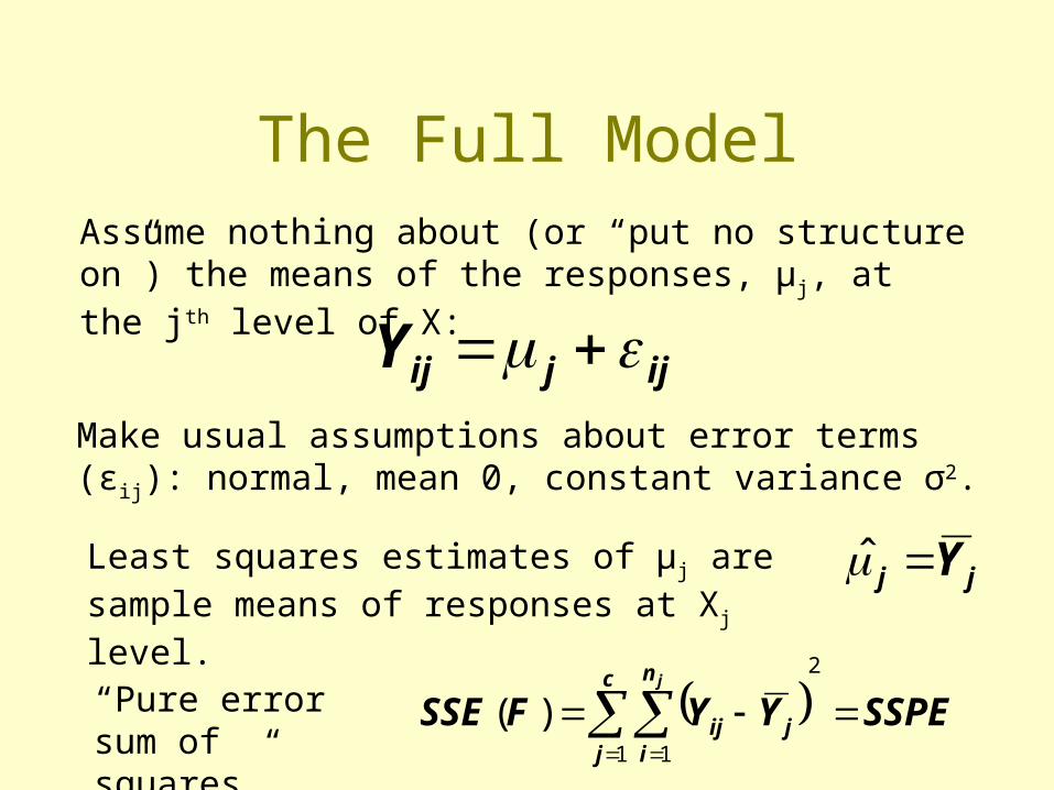
The Full ModelAssume nothing about (or “put no structure on”) the means of the responses, μj, at the jth level of X:

ijjijY Make usual assumptions about error terms (εij): normal, mean 0, constant variance σ2.

Least squares estimates of μj are sample means of responses at Xj level.

jj Y

“Pure error sum of squares”

SSPEYYFSSEc

j

n

ijij

j

2

1 1

)(

The Reduced ModelAssume the means of the responses, μj, are linearly related to the jth level of X (same model as before, just modified subscripts):

ijjij XY 10

Make usual assumptions about error terms (εij): normal, mean 0, constant variance σ2.

Least squares estimates of μj are as usual. jij XbbY 10ˆ

“Error sum of squares” SSEYYRSSEc

j

n

iijij

j

2

1 1

ˆ)(

Error sum of squares decomposition

ijjjijijij YYYYYY ˆˆ error deviation pure error deviation lack of fit deviation

j i

ijjj i

jijj i

ijij YYYYYY222 ˆˆ

SSLFSSPESSE

The F test

FFR df

FSSE

dfdf

FSSERSSEF

)()()(*

2ndfRcndfF

SSERSSE )(

SSPEFSSE )(

MSPE

MSLF

n

SSPE

c

SSLF

n

SSPE

cnn

SSPESSEF

2222*

The Decision (Intuitively)

• If the largest portion of the error sum of squares is due to lack of fit, the F test should be large.

• A large F* statistic leads to a small P-value (determined by F(c-2, n-2) distribution).

• If P-value is small, reject null and conclude significant lack of (linear) fit.

LOF Test summarized in an ANOVA Table

LOF Test in Minitab

• Stat >> Regression >> Regression …

• Specify predictor and response.

• Under Options…, under Lack of Fit Tests, select box labeled “Pure error.”

• Select OK. Select OK. ANOVA table appears in session window.

504030

200

150

100

Latitude

Mo

rtal

ityS = 19.1150 R-Sq = 68.0 % R-Sq(adj) = 67.3 %

Mortality = 389.189 - 5.97764 Latitude

Regression Plot

Example 1

Do the data suggest that a linear function is adequate in describing the relationship between skin cancer mortality and latitude?

Example 1: Mortality and Latitude

Analysis of Variance

Source DF SS MS F PRegression 1 36464 36464 99.80 0.000Residual Error 47 17173 365 Lack of Fit 30 12863 429 1.69 0.128 Pure Error 17 4310 254Total 48 53637

19 rows with no replicates

Example 2

Do the data suggest that a linear function is adequate in describing the relationship between the length and weight of an alligator?

150140130120110100 90 80 70 60

700

600

500

400

300

200

100

0

Length

Wei

ght

S = 54.0115 R-Sq = 83.6 % R-Sq(adj) = 82.9 %

Weight = -393.264 + 5.90235 Length

Regression Plot

Example 2: Alligator length and weight

Analysis of Variance

Source DF SS MS F PRegression 1 342350 342350 117.35 0.000Residual Error 23 67096 2917 Lack of Fit 17 66567 3916 44.36 0.000 Pure Error 6 530 88Total 24 409446

14 rows with no replicates

Example 3

Do the data suggest that a linear function is adequate in describing the relationship between iron content and weight loss due to corrosion?

210

130

120

110

100

90

80

iron

wgt

loss

S = 3.05778 R-Sq = 97.0 % R-Sq(adj) = 96.7 %

wgtloss = 129.787 - 24.0199 iron

Regression Plot

Example 3: Iron and corrosion

Analysis of Variance

Source DF SS MS F PRegression 1 3293.8 3293.8 352.27 0.000Residual Error 11 102.9 9.4 Lack of Fit 5 91.1 18.2 9.28 0.009 Pure Error 6 11.8 2.0Total 12 3396.6

2 rows with no replicates

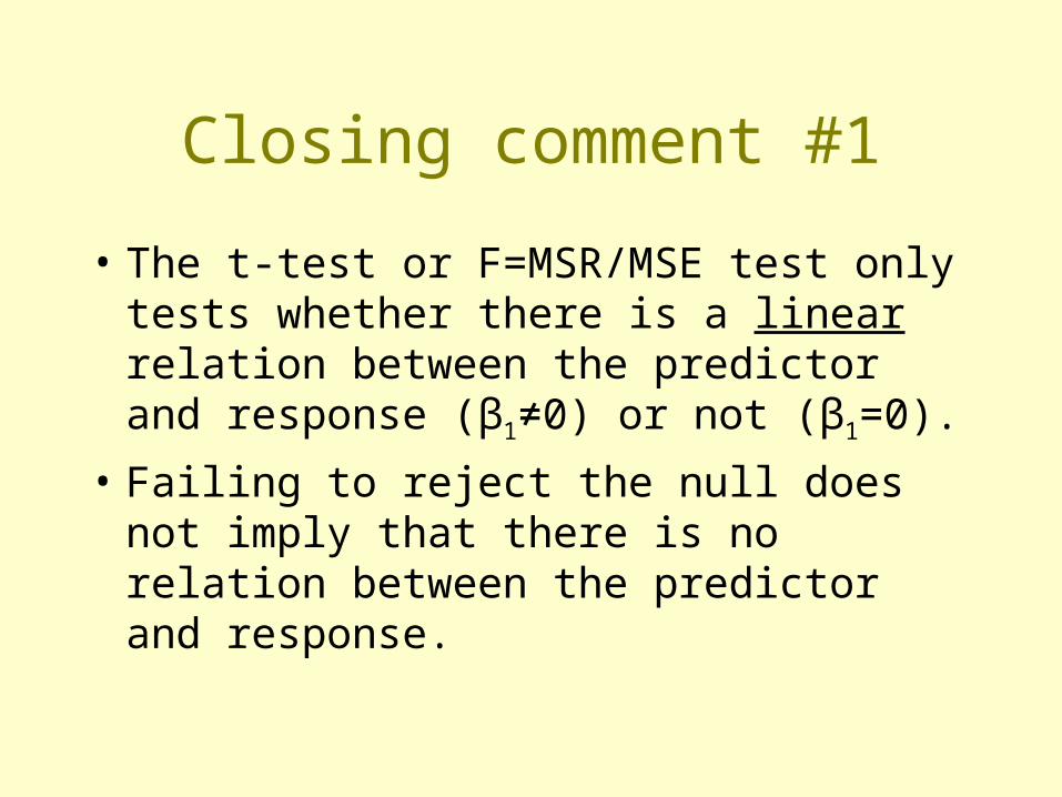
Closing comment #1

• The t-test or F=MSR/MSE test only tests whether there is a linear relation between the predictor and response (β1≠0) or not (β1=0).

• Failing to reject the null does not imply that there is no relation between the predictor and response.

50-5

40

30

20

10

0

X

Y*

Example: Closing comment #1

Example: Closing comment #1The regression equation isY* = 14.1 - 0.100 X

Predictor Coef SE Coef T PConstant 14.118 2.598 5.44 0.000X -0.0998 0.6942 -0.14 0.887

S = 13.25 R-Sq = 0.1% R-Sq(adj) = 0.0%

Analysis of VarianceSource DF SS MS F PRegression 1 3.6 3.6 0.02 0.887Residual Error 24 4210.4 175.4 Lack of Fit 11 4188.3 380.8 223.87 0.000 Pure Error 13 22.1 1.7Total 25 4214.0

Closing comments #2, #3

• We used general linear test approach to test appropriateness of a linear function. It can just as easily be used to test for appropriateness of other functions (quadratic, cubic).

• The alternative HA: Lack of fit (not linear) includes all possible regression functions other than a linear one. Use residuals to help identify what type of function is appropriate.