Embed Size (px)
Citation preview
University of TrentoFaculty of Mathematical, Physical and Natural Sciences
Master of Science in Computer Science
Department of Engineering and Computer ScienceDISI
NOTES FOR THE COURSE
Laboratory of Embedded Control Systems
Luigi Palopoli and Daniele Fontanelli
Abstract
The aim of this notes is to mainly cover all the theoretical aspects of the course of Laboratory ofEmbedded Control Systems. Practical insight on the relevant aspects of the project development willalso be covered. However, most of the practical issues related to the use of the robotic platform (i.e.,the Lego Mindstorm), on the real–time embedded kernel to be adopted (i.e., NXT Osek) and on thechosen simulation and design software (i.e., Scicos Lab) will be referenced throughout these notes.
2
Contents
1 Introduction and Background Material 5
1.1 The Course . . . . . . . . . . . . . . . . . . . . . . . . . . . . . . . . . . . . . . . . . 5
1.2 Brief Introduction to Scicoslab . . . . . . . . . . . . . . . . . . . . . . . . . . . . . . . 6
1.2.1 Command Window . . . . . . . . . . . . . . . . . . . . . . . . . . . . . . . . . 6
1.2.2 Vectors and Matrices . . . . . . . . . . . . . . . . . . . . . . . . . . . . . . . . 7
1.2.3 Strings . . . . . . . . . . . . . . . . . . . . . . . . . . . . . . . . . . . . . . . . 8
1.2.4 Scicoslab Programming . . . . . . . . . . . . . . . . . . . . . . . . . . . . . . . 8
1.2.5 Scicos . . . . . . . . . . . . . . . . . . . . . . . . . . . . . . . . . . . . . . . . 13
1.2.6 Scicoslab references . . . . . . . . . . . . . . . . . . . . . . . . . . . . . . . . . 18
1.3 The Lego Mindstorm . . . . . . . . . . . . . . . . . . . . . . . . . . . . . . . . . . . . 18
1.4 Bibliography . . . . . . . . . . . . . . . . . . . . . . . . . . . . . . . . . . . . . . . . . 19
2 The Laplace Transform 21
2.1 Bilateral L-transform . . . . . . . . . . . . . . . . . . . . . . . . . . . . . . . . . . . . 21
2.2 Unilateral L-transform and ROC . . . . . . . . . . . . . . . . . . . . . . . . . . . . . 25
2.3 Inverse L-transform . . . . . . . . . . . . . . . . . . . . . . . . . . . . . . . . . . . . . 26
2.4 Properties of a Signal given the L-transform . . . . . . . . . . . . . . . . . . . . . . . 26
2.5 Bibliography . . . . . . . . . . . . . . . . . . . . . . . . . . . . . . . . . . . . . . . . . 28
3 Modeling and Identification 29
3.1 Dynamic Systems . . . . . . . . . . . . . . . . . . . . . . . . . . . . . . . . . . . . . . 29
3.1.1 Fundamental Properties of Dynamic Systems . . . . . . . . . . . . . . . . . . . 32
3.1.2 Impulse Response . . . . . . . . . . . . . . . . . . . . . . . . . . . . . . . . . . 34
3.2 Analysis of a Linear System . . . . . . . . . . . . . . . . . . . . . . . . . . . . . . . . 34
3.2.1 System with Divergent Behaviors . . . . . . . . . . . . . . . . . . . . . . . . . 35
3.2.2 First Order Systems . . . . . . . . . . . . . . . . . . . . . . . . . . . . . . . . 37
3.2.3 Second Order Systems . . . . . . . . . . . . . . . . . . . . . . . . . . . . . . . 41
3.3 Motor model . . . . . . . . . . . . . . . . . . . . . . . . . . . . . . . . . . . . . . . . 46
3.4 Identification . . . . . . . . . . . . . . . . . . . . . . . . . . . . . . . . . . . . . . . . 47
3.4.1 Time Domain Approach . . . . . . . . . . . . . . . . . . . . . . . . . . . . . . 47
3.4.2 Frequency Domain Approach . . . . . . . . . . . . . . . . . . . . . . . . . . . 49
3.5 Bibliography . . . . . . . . . . . . . . . . . . . . . . . . . . . . . . . . . . . . . . . . . 50
3
4 CONTENTS
4 Control Design 514.1 Feedback Paradigm . . . . . . . . . . . . . . . . . . . . . . . . . . . . . . . . . . . . . 51
4.1.1 The Example of the Electric Heater . . . . . . . . . . . . . . . . . . . . . . . . 524.1.2 The Example of the DC Brushless Motor . . . . . . . . . . . . . . . . . . . . . 554.1.3 The Closed Loop . . . . . . . . . . . . . . . . . . . . . . . . . . . . . . . . . . 55
4.2 Basic Concept of Stability . . . . . . . . . . . . . . . . . . . . . . . . . . . . . . . . . 564.2.1 Linear Time–Invariant System Stability . . . . . . . . . . . . . . . . . . . . . . 58
4.3 Feedback Design for Linear Systems . . . . . . . . . . . . . . . . . . . . . . . . . . . . 604.4 Root Locus . . . . . . . . . . . . . . . . . . . . . . . . . . . . . . . . . . . . . . . . . 65
4.4.1 Root locus construction . . . . . . . . . . . . . . . . . . . . . . . . . . . . . . 674.4.2 Analysis of a Second Order System in the Root Locus . . . . . . . . . . . . . . 72
4.5 Bibliography . . . . . . . . . . . . . . . . . . . . . . . . . . . . . . . . . . . . . . . . . 73
5 Digital Control 745.1 Discretization of Linear Continuous Time Controllers . . . . . . . . . . . . . . . . . . 74
5.1.1 Approximation of the Integral . . . . . . . . . . . . . . . . . . . . . . . . . . . 755.1.2 Hints . . . . . . . . . . . . . . . . . . . . . . . . . . . . . . . . . . . . . . . . . 78
5.2 Multitask Implementation . . . . . . . . . . . . . . . . . . . . . . . . . . . . . . . . . 785.3 Bibliography . . . . . . . . . . . . . . . . . . . . . . . . . . . . . . . . . . . . . . . . . 79
6 Simulation and Control of a Wheeled Robot 836.1 Kinematic Model of the Robot . . . . . . . . . . . . . . . . . . . . . . . . . . . . . . . 83
6.1.1 Wagon Constrained on a Linear Track . . . . . . . . . . . . . . . . . . . . . . 856.1.2 Wagon Constrained on a Circular Track . . . . . . . . . . . . . . . . . . . . . 866.1.3 The Unicycle Vehicle . . . . . . . . . . . . . . . . . . . . . . . . . . . . . . . . 87
6.2 Kinematic Linear Control . . . . . . . . . . . . . . . . . . . . . . . . . . . . . . . . . 896.2.1 Estimation Algorithms and Observers . . . . . . . . . . . . . . . . . . . . . . . 90
6.3 Bibliography . . . . . . . . . . . . . . . . . . . . . . . . . . . . . . . . . . . . . . . . . 90
Chapter 1
Introduction and Background Material
This Chapter describes the structure of the course and summarizes the fundamental concepts assumedto be already known by the students.
1.1 The Course
The course of Laboratory of Embedded Control Systems is not a course on Automatic Control, nora course on Real–Time control and definitely not a course on Digital Control. However, the basicknowledge of all the previously mentioned Engineering areas are needed to successfully complete theassigned project.
In fact, this course is a project course in which the development of a practical real systemand the way to achieve it constitute the basis of the exam test. More precisely, starting from theknowledge gained during the course of Signals and Systems, the students will be guided throughthe so called Model Based Design paradigm. In practice, given a mathematical model of a genericsystem (or plant), with the Model Based Design it is possible to synthesize a control law that is ableto modify the behavior of the plant according to some predefined performance indices. The systemconsidered in this course is a wheeled mobile robot to be assembled with the Lego Mindstorm kitsthat are available. Basically, the students have to: 1) derive a mathematical model the robot (andits components, i.e., actuators, sensors, motion constraints); 2) identify the physical parameters ofthe model; 3) formulate design specifications and performance targets for the modelled system; 4)design proper control laws in order to fullfil the pre-specified goals; 5) simulate the system subjectedto the control law to assess its performance, limits and adherence to the specifications; 6) generate asoftware implementation of the controller implementing the control law and finally 7) test the overallsystem on the field.
Therefore, in order to fullfil the stimulating challenges of this course, the students will be guidedthrough the following scheduled steps:
1. Understanding the use of Scicoslab. We will give first a brief description of the adopted tool(Section 1.2), then it will be used throughout these notes to show how the theory can be appliedin practice;
2. Approaching the mechanical platform (Section 1.3);
3. Recap on Laplace Transform (Chapter 2);
5

6 CHAPTER 1. INTRODUCTION AND BACKGROUND MATERIAL
4. Modeling systems, such as actuators and sensors, and learn how to identifies their physicalparameters (Chapter 3);
5. Control law design techniques for Single Input Single Output (SISO) systems (Chapter 4);
6. Digital control design (Chapter 5);
7. Simulation and control design for a complex system like a wheeled mobile robot (Chapter 6);
8. Practical digital implementation (Section 5.2) and test on the field.
Throughout these notes, a list of reference books and materials will be given on purpose. In thisintroductory section, we simply list some books that explains the basic concepts compounding theModel Based Design paradigm that can be used as reference. For linear systems and control, wecan suggest [PPR03] and [Kai80]. Two books are mainly related to the joint world of control designand digital implementation, which are [Oga95] and [AW96]. For what concern robot modeling andcontrol, a useful book is [SSVO08].
1.2 Brief Introduction to Scicoslab
Scicoslab is a free scientific software package for numerical computations, modeling and simulation ofdynamical systems, data processing and statistics providing a powerful open computing environmentfor engineering and scientific applications (see [Groc] and [Grob]). Scicoslab is an open sourcesoftware. Since 1994 it has been distributed freely along with the source code via the Internet. Itis currently used in educational and industrial environments around the world. It includes hundredsof mathematical functions with the possibility to add interactively programs from various languages(C, C++, Fortran...). It has sophisticated data structures (including lists, polynomials, rationalfunctions, linear systems...), an interpreter and a high level programming language.
Scicoslab is quite similar to Matlab, and the range of functions are comparable. The largestbenefit of Scicoslab is of course that it is free. Additional similarities are with Octave, which is alsofree, but Scicoslab comes with Scicos, which is automatically installed with Scicoslab. Scicos is ablock-diagram based simulation tool similar to Simulink and LabVIEW Simulation Module, and it isable to easily implement Hardware In the Loop simulations as well as interface with external devices.
1.2.1 Command Window
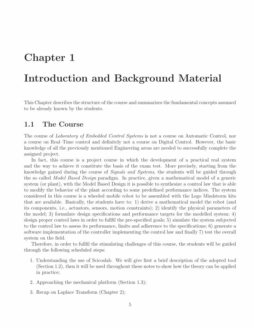
Starting Scicoslab, it opens a command window (Fig. 1.1). Scicoslab commands are executed at thecommand line by entering the command, and then clicking the Enter button on the keyboard.
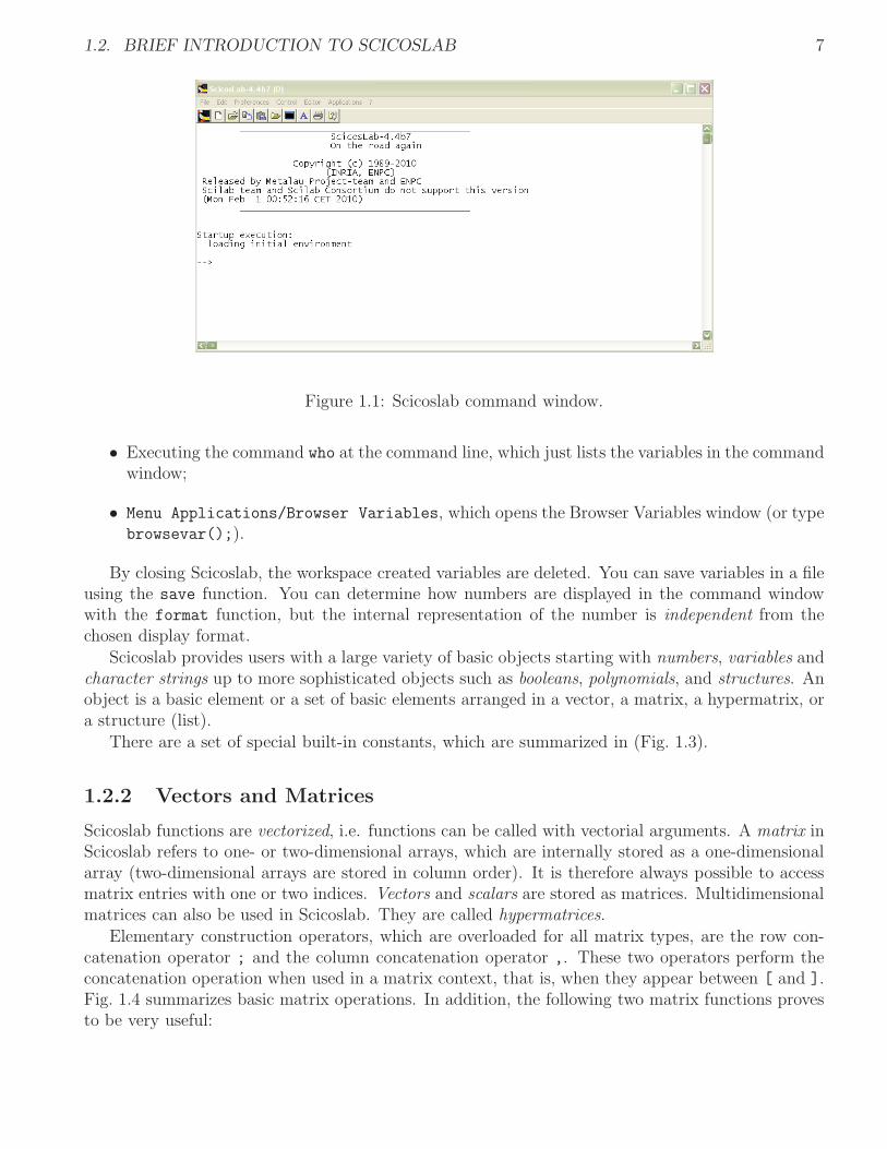
Typing help the help browser appears (Fig. 1.2). You can type help and the name of a command(or apropos and the name of a command) to get directly to the help of the desired command.
Variables are defined by simply assigning them the result of an operation. Using ; at the end ofan operation avoid the output to be shown. Using , in the command line allow the execution of morethan one command sequentially. Scicoslab is case sensitive, i.e., a and A are two different variables.Typing the name of a variable in the command window, the variable exists in the workspace.
There are two ways to see the contents of the workspace:
1.2. BRIEF INTRODUCTION TO SCICOSLAB 7
Figure 1.1: Scicoslab command window.
• Executing the command who at the command line, which just lists the variables in the commandwindow;
• Menu Applications/Browser Variables, which opens the Browser Variables window (or typebrowsevar();).
By closing Scicoslab, the workspace created variables are deleted. You can save variables in a fileusing the save function. You can determine how numbers are displayed in the command windowwith the format function, but the internal representation of the number is independent from thechosen display format.
Scicoslab provides users with a large variety of basic objects starting with numbers, variables andcharacter strings up to more sophisticated objects such as booleans, polynomials, and structures. Anobject is a basic element or a set of basic elements arranged in a vector, a matrix, a hypermatrix, ora structure (list).
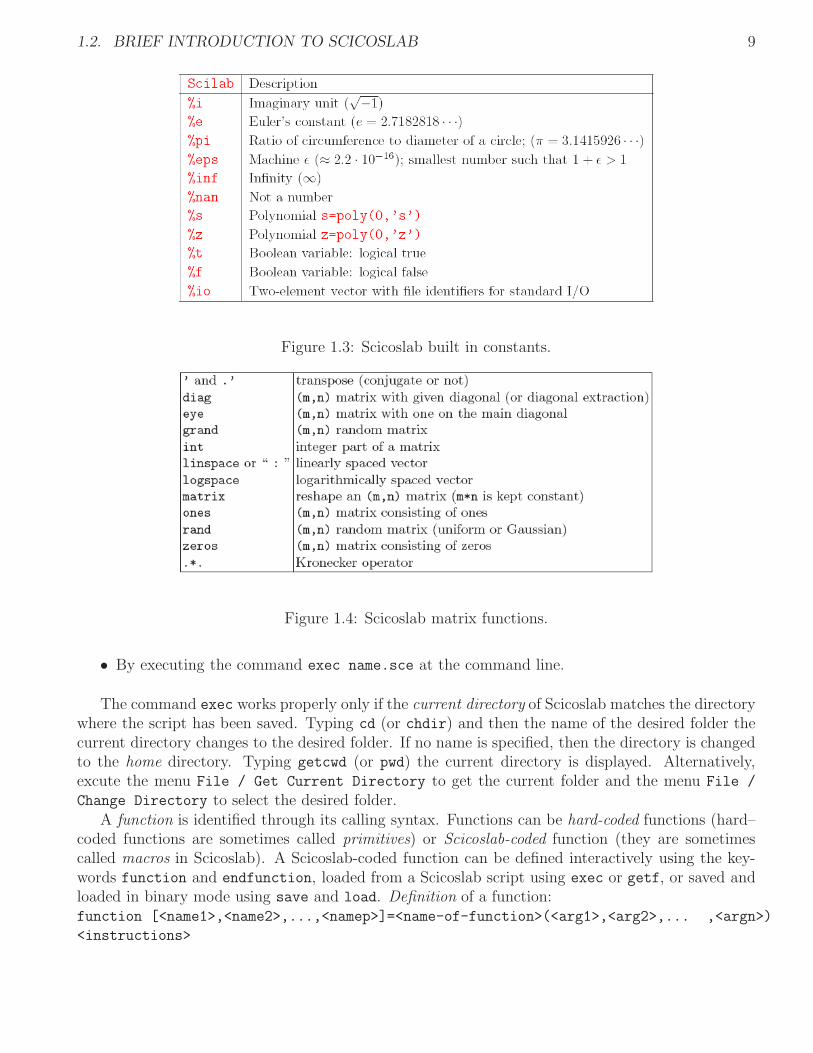
There are a set of special built-in constants, which are summarized in (Fig. 1.3).
1.2.2 Vectors and Matrices
Scicoslab functions are vectorized, i.e. functions can be called with vectorial arguments. A matrix inScicoslab refers to one- or two-dimensional arrays, which are internally stored as a one-dimensionalarray (two-dimensional arrays are stored in column order). It is therefore always possible to accessmatrix entries with one or two indices. Vectors and scalars are stored as matrices. Multidimensionalmatrices can also be used in Scicoslab. They are called hypermatrices.
Elementary construction operators, which are overloaded for all matrix types, are the row con-catenation operator ; and the column concatenation operator ,. These two operators perform theconcatenation operation when used in a matrix context, that is, when they appear between [ and ].Fig. 1.4 summarizes basic matrix operations. In addition, the following two matrix functions provesto be very useful:
8 CHAPTER 1. INTRODUCTION AND BACKGROUND MATERIAL
Figure 1.2: Scicoslab help window.
• The function size returns the dimension of a matrix;
• The function length returns the length of a matrix (i.e., the overall number of entries).
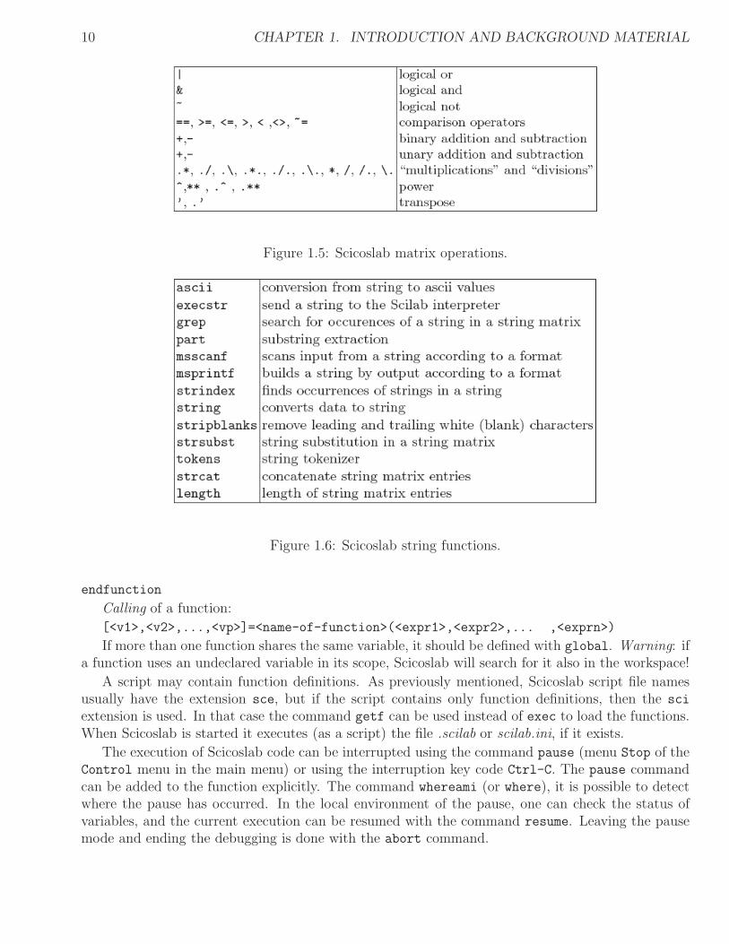
Moreover, a set of matrix operators is reported in Fig. 1.5. Furthermore, the operator $ returnsthe index of the last element of a matrix.
1.2.3 Strings
Strings in Scicoslab are delimited by either single ’ or double quotes ", which are equivalent. If oneof these two characters is to be inserted in a string, it has to be preceded by a delimiter, which isagain a single or double quote. Basic operations on strings are the concatenation (operator “+”)and the function length. A string is just a 1x1 string matrix whose type is denoted by “string” (asreturned by typeof). A brief list of string functions is offered in Fig. 1.6.
1.2.4 Scicoslab Programming
A Scicoslab script is a text file of name *.sce containing commands. Editing of scripts can becarried out using the Scipad editor (type Scipad or use the menu). Scripts can also have extensionsci, however the default extension when saving a script file in Scipad is sce. It is very useful touse scripts even for small set of operations because the project is saved in files which is good fordocumentation and very convenient for debug and repeated executions. Line starting with \\ areconsidered as comments.
There are two ways to execute the name.sce script:
• With the Execute / Load into Scicoslab menu in Scipad;
1.2. BRIEF INTRODUCTION TO SCICOSLAB 9
Figure 1.3: Scicoslab built in constants.
Figure 1.4: Scicoslab matrix functions.
• By executing the command exec name.sce at the command line.
The command exec works properly only if the current directory of Scicoslab matches the directorywhere the script has been saved. Typing cd (or chdir) and then the name of the desired folder thecurrent directory changes to the desired folder. If no name is specified, then the directory is changedto the home directory. Typing getcwd (or pwd) the current directory is displayed. Alternatively,excute the menu File / Get Current Directory to get the current folder and the menu File /
Change Directory to select the desired folder.A function is identified through its calling syntax. Functions can be hard-coded functions (hard–
coded functions are sometimes called primitives) or Scicoslab-coded function (they are sometimescalled macros in Scicoslab). A Scicoslab-coded function can be defined interactively using the key-words function and endfunction, loaded from a Scicoslab script using exec or getf, or saved andloaded in binary mode using save and load. Definition of a function:function [<name1>,<name2>,...,<namep>]=<name-of-function>(<arg1>,<arg2>,... ,<argn>)
<instructions>
10 CHAPTER 1. INTRODUCTION AND BACKGROUND MATERIAL
Figure 1.5: Scicoslab matrix operations.
Figure 1.6: Scicoslab string functions.
endfunction
Calling of a function:
[<v1>,<v2>,...,<vp>]=<name-of-function>(<expr1>,<expr2>,... ,<exprn>)
If more than one function shares the same variable, it should be defined with global. Warning: ifa function uses an undeclared variable in its scope, Scicoslab will search for it also in the workspace!
A script may contain function definitions. As previously mentioned, Scicoslab script file namesusually have the extension sce, but if the script contains only function definitions, then the sci
extension is used. In that case the command getf can be used instead of exec to load the functions.When Scicoslab is started it executes (as a script) the file .scilab or scilab.ini, if it exists.
The execution of Scicoslab code can be interrupted using the command pause (menu Stop of theControl menu in the main menu) or using the interruption key code Ctrl-C. The pause commandcan be added to the function explicitly. The command whereami (or where), it is possible to detectwhere the pause has occurred. In the local environment of the pause, one can check the status ofvariables, and the current execution can be resumed with the command resume. Leaving the pausemode and ending the debugging is done with the abort command.
1.2. BRIEF INTRODUCTION TO SCICOSLAB 11
In the following, a list of basic programming instructions:
Branching :
• if <condition> then
<instructions>
else
<instructions>
end
• select <expr> ,
case <expr1> then
<instructions>
case <expr2> then
<instructions>
...
else
<instructions>
end
Iterations :
• for <name>=<expr>
<instructions>
end
• while <condition>
<instructions>
end
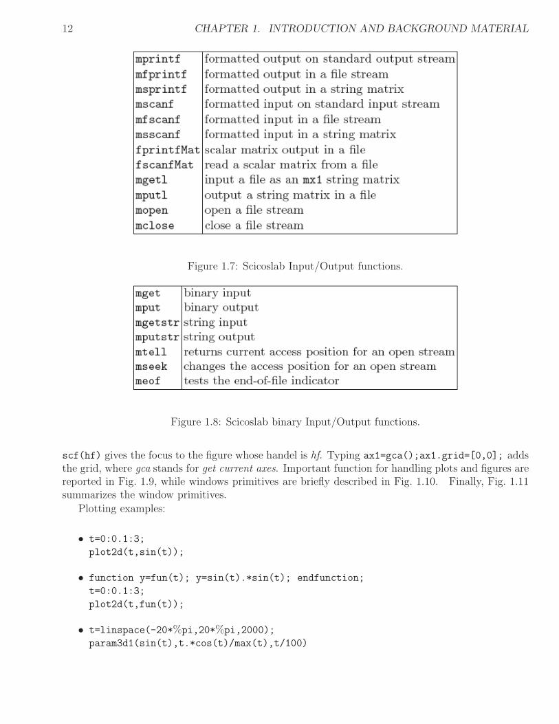
The presence of a break statement in the <instructions> ends the loop.For basic data input/output, follows the functions in Fig. 1.7). Several Scicoslab functions can
used to perform formatted input-output. The functions write and read are based on Fortranformatted input and output. They redirect input and output to streams, which are obtained throughthe use of the function file.
Scicoslab has its own binary internal format for saving Scicoslab objects and Scicoslab graphicsin a machine-independent way. It is possible to save variables in a binary file from the currentenvironment using the command save. A set of saved variables can be loaded in a running Scicoslabenvironment with the load command. A list of binary input/output functions is given in Fig. 1.8.
Plotting
The basic command for plotting data in a figure is plot2d. The properties of the graph (as well asof each entity in Scicoslab) can be obtained using the get command. Then, each property is madeaccessible and can be modified by the user. In the Graphics window menu it is possible to click onthe GED button, which opens the Graphics Editor.
To create a figure type hf = scf(n), where n is the identifier and hf is the figure handle. Thelatter specify the plot to be modified. For example, clf(hf) clears the figure whose handel is hf, while
12 CHAPTER 1. INTRODUCTION AND BACKGROUND MATERIAL
Figure 1.7: Scicoslab Input/Output functions.
Figure 1.8: Scicoslab binary Input/Output functions.
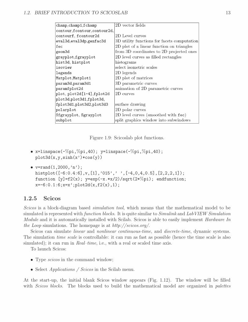
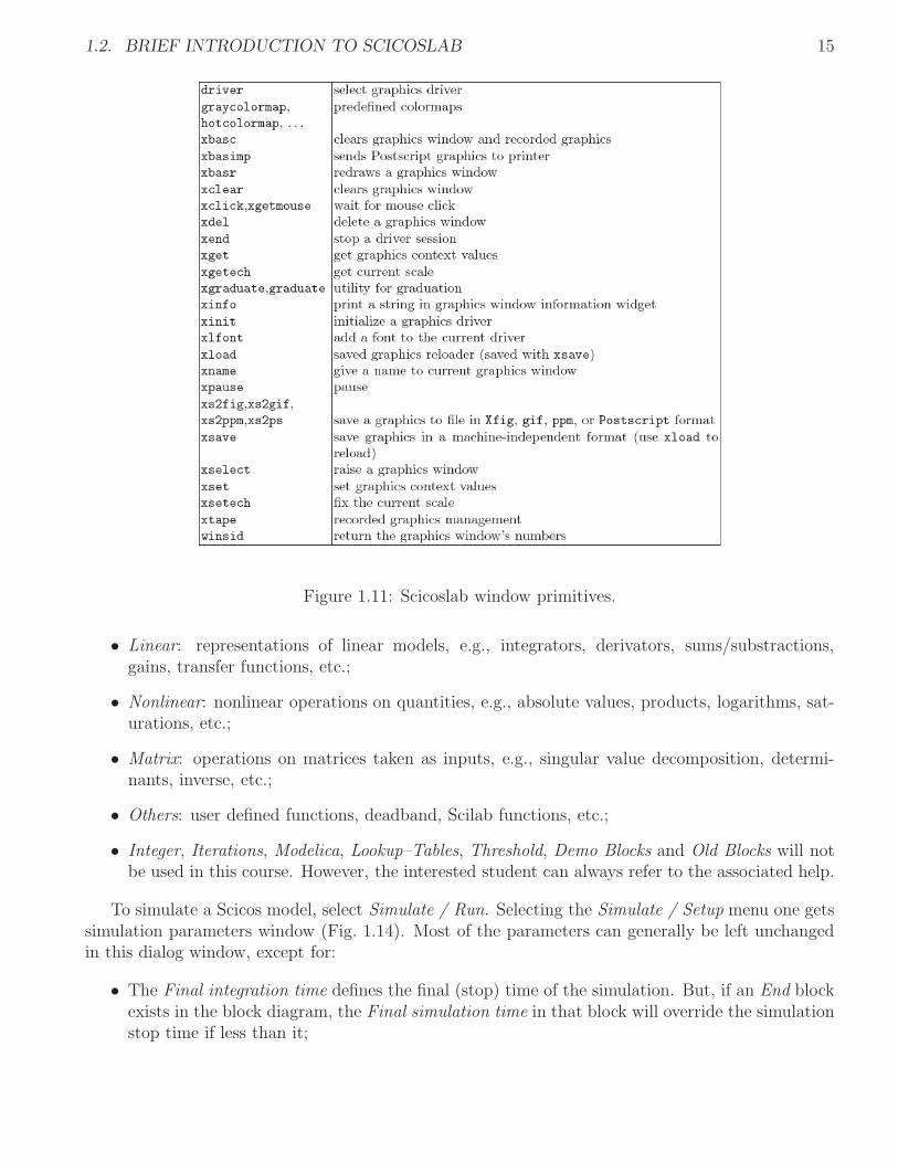
scf(hf) gives the focus to the figure whose handel is hf. Typing ax1=gca();ax1.grid=[0,0]; addsthe grid, where gca stands for get current axes. Important function for handling plots and figures arereported in Fig. 1.9, while windows primitives are briefly described in Fig. 1.10. Finally, Fig. 1.11summarizes the window primitives.
Plotting examples:
• t=0:0.1:3;
plot2d(t,sin(t));
• function y=fun(t); y=sin(t).*sin(t); endfunction;
t=0:0.1:3;
plot2d(t,fun(t));
• t=linspace(-20*%pi,20*%pi,2000);
param3d1(sin(t),t.*cos(t)/max(t),t/100)
1.2. BRIEF INTRODUCTION TO SCICOSLAB 13
Figure 1.9: Scicoslab plot functions.
• x=linspace(-%pi,%pi,40); y=linspace(-%pi,%pi,40);
plot3d(x,y,sinh(x’)*cos(y))
• v=rand(1,2000,’n’);
histplot([-6:0.4:6],v,[1],’015’,’ ’,[-4,0,4,0.5],[2,2,2,1]);
function [y]=f2(x); y=exp(-x.*x/2)/sqrt(2*%pi); endfunction;
x=-6:0.1:6;x=x’;plot2d(x,f2(x),1);
1.2.5 Scicos
Scicos is a block-diagram based simulation tool, which means that the mathematical model to besimulated is represented with function blocks. It is quite similar to Simulink and LabVIEW SimulationModule and it is automatically installed with Scilab. Scicos is able to easily implement Hardware Inthe Loop simulations. The homepage is at http://scicos.org/.
Scicos can simulate linear and nonlinear continuous-time, and discrete-time, dynamic systems.The simulation time scale is controllable: it can run as fast as possible (hence the time scale is alsosimulated); it can run in Real–time, i.e., with a real or scaled time axis.
To launch Scicos:
• Type scicos in the command window;
• Select Applications / Scicos in the Scilab menu.
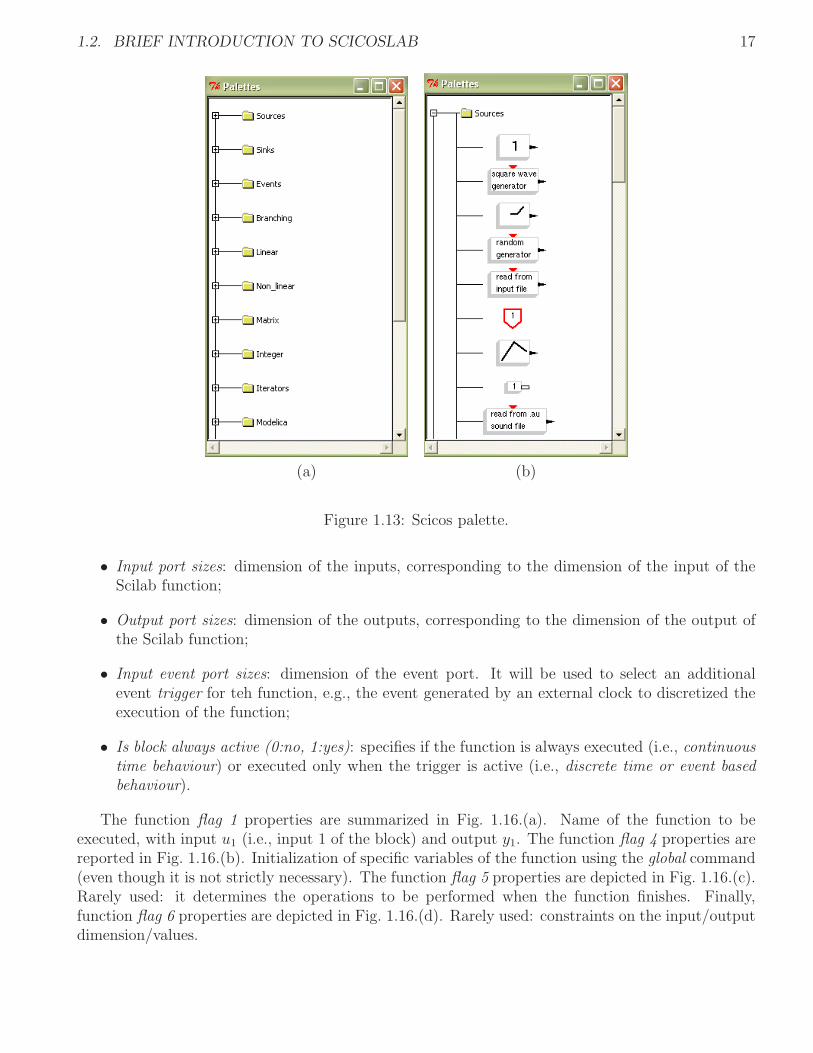
At the start-up, the initial blank Scicos window appears (Fig. 1.12). The window will be filledwith Scicos blocks. The blocks used to build the mathematical model are organized in palettes

14 CHAPTER 1. INTRODUCTION AND BACKGROUND MATERIAL
Figure 1.10: Scicoslab graphics primitives.
(Fig. 1.13.(a)). To display the palettes in a tree structure, select Palettes / Pal tree in the Scicosmenu. To see the individual blocks on a specific palette, click the plus sign in front of the palette(Fig. 1.13.(b)). Alternatively, select the desired palette via the Palette / Palettes menu. Right–clicking on each element of the palette, i.e., on each Scicos block, a pop–up menu opens, with threedifferent choices:
• Place in Diagram: places the block in the Scicos window, where it can be moved freely. Alter-natively, you can drag–and–drop the element in the Scicos window directly;
• Help: gets the Scilab help for the specified block;
• Details: shows the details of the block, e.g., number of inputs, number of outputs, etc..
• Sources: various signals generators that are the inputs to the model;
• Sinks: various visualizations of signals, that are the output variables of interest;
• Events: event generators for the model;
• Branching: blocks performing the routing of the signals in the model,e.g., multiplexers, demul-tiplexers, switch, buses, etc.;
1.2. BRIEF INTRODUCTION TO SCICOSLAB 15
Figure 1.11: Scicoslab window primitives.
• Linear: representations of linear models, e.g., integrators, derivators, sums/substractions,gains, transfer functions, etc.;
• Nonlinear: nonlinear operations on quantities, e.g., absolute values, products, logarithms, sat-urations, etc.;
• Matrix: operations on matrices taken as inputs, e.g., singular value decomposition, determi-nants, inverse, etc.;
• Others: user defined functions, deadband, Scilab functions, etc.;
• Integer, Iterations, Modelica, Lookup–Tables, Threshold, Demo Blocks and Old Blocks will notbe used in this course. However, the interested student can always refer to the associated help.
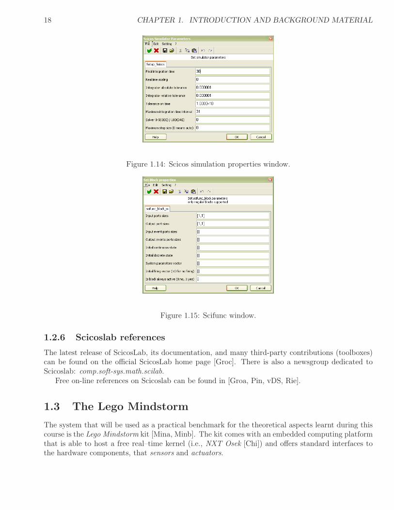
To simulate a Scicos model, select Simulate / Run. Selecting the Simulate / Setup menu one getssimulation parameters window (Fig. 1.14). Most of the parameters can generally be left unchangedin this dialog window, except for:
• The Final integration time defines the final (stop) time of the simulation. But, if an End blockexists in the block diagram, the Final simulation time in that block will override the simulationstop time if less than it;

16 CHAPTER 1. INTRODUCTION AND BACKGROUND MATERIAL
Figure 1.12: Scicos initial window (blank sheet).
• The Realtime scaling parameter defines the relative speed of the real time compared to thesimulated time. For example, if Realtime scaling is 0.2, the real time runs 0.2 times as fast asthe simulated time. In other words, the simulator runs 1/0.2 = 5 times faster than real time.You can use this parameter to speed up or slow down the simulator;
• The maximum step size can be set to a proper value. As a rule of thumb, one tenth of thequickest time-constant (or apparent time-constant) of the system to be simulated;
• The solvermethod (i.e. the numerical method that Scicos uses to solve the underlying algebraicand differential equations making up the model) can be selected via the solver parameter, butin most cases the default solver can be accepted;
• The time scale fo the simulation is defined by the user and the particular application to simulate(e.g., a mass flow parameter can be given in kg/s or kg/min). However the choice of the secondsis suggested.
Model parameters and simulation parameters can be set in the Context of the simulator. For,select Diagram / Context from the Scicos menu bar. The Context is simply represented by a numberof Scilab expressions defining the parameters (or variables) and assigning them values (the use ofthe command global is appreciated). These parameters are used throughout the Scicos diagram, e.g.,blocks, user defined functions, etc.
The Scifunc
Scilab coded functions can be executed as Scicos blocks, i.e., Scifunc. When the Scifunc is placedin the Scicos window, it is possible to visualize its properties. Double–clicking on the Scifunc block,the first property window is visualized (Fig. 1.15).
1.2. BRIEF INTRODUCTION TO SCICOSLAB 17
(a) (b)
Figure 1.13: Scicos palette.
• Input port sizes: dimension of the inputs, corresponding to the dimension of the input of theScilab function;
• Output port sizes: dimension of the outputs, corresponding to the dimension of the output ofthe Scilab function;
• Input event port sizes: dimension of the event port. It will be used to select an additionalevent trigger for teh function, e.g., the event generated by an external clock to discretized theexecution of the function;
• Is block always active (0:no, 1:yes): specifies if the function is always executed (i.e., continuoustime behaviour) or executed only when the trigger is active (i.e., discrete time or event basedbehaviour).
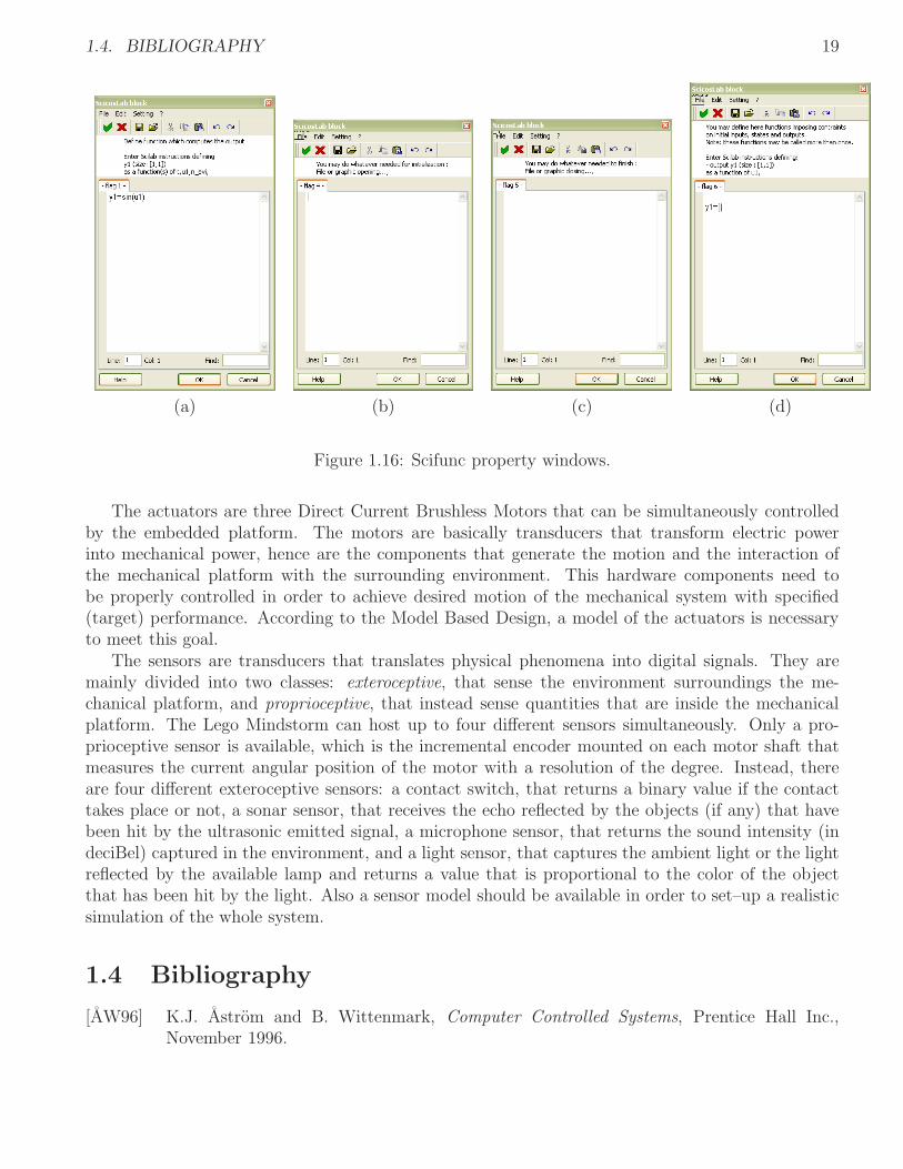
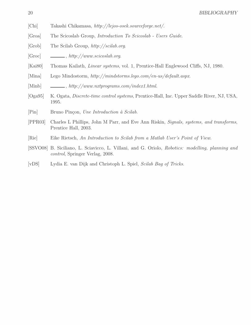
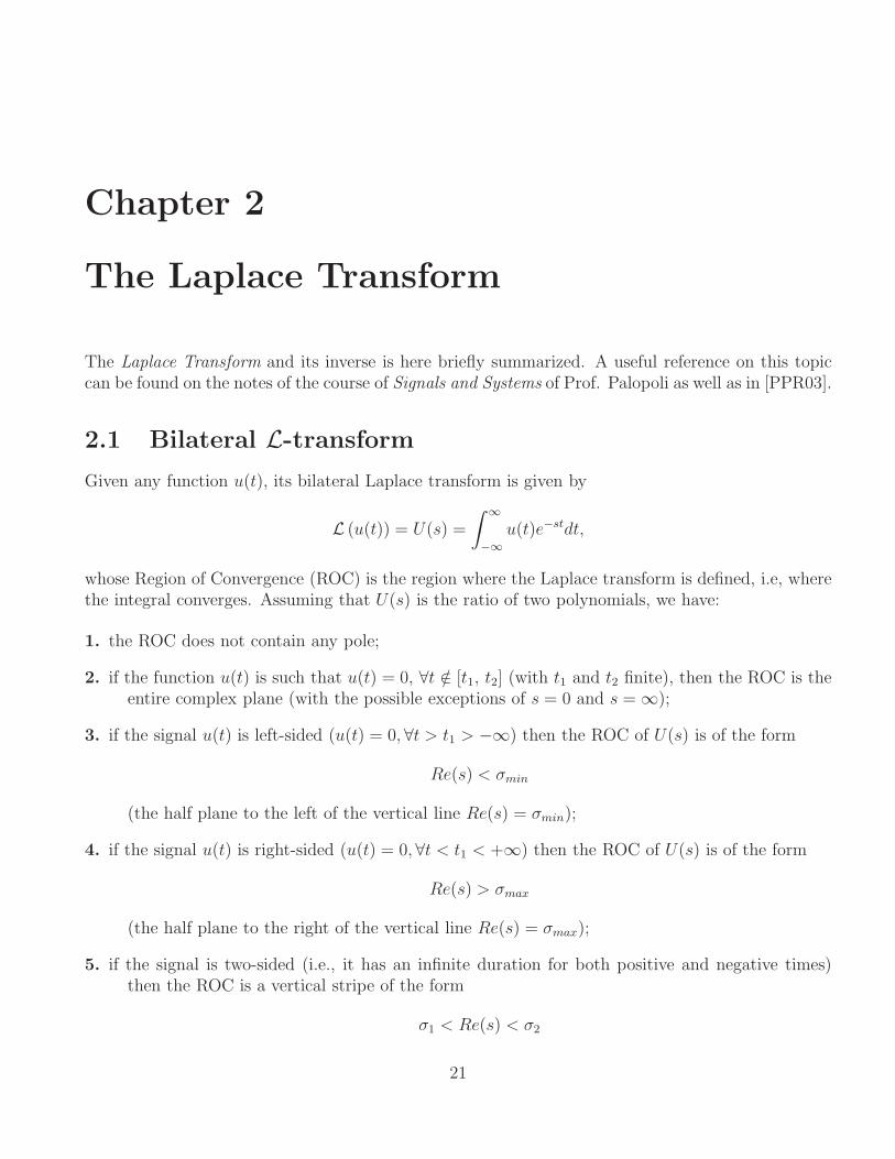
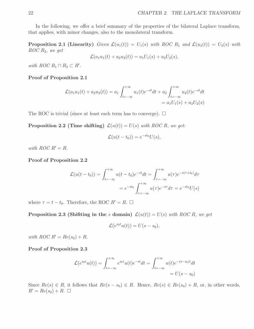
The function flag 1 properties are summarized in Fig. 1.16.(a). Name of the function to beexecuted, with input u1 (i.e., input 1 of the block) and output y1. The function flag 4 properties arereported in Fig. 1.16.(b). Initialization of specific variables of the function using the global command(even though it is not strictly necessary). The function flag 5 properties are depicted in Fig. 1.16.(c).Rarely used: it determines the operations to be performed when the function finishes. Finally,function flag 6 properties are depicted in Fig. 1.16.(d). Rarely used: constraints on the input/outputdimension/values.
18 CHAPTER 1. INTRODUCTION AND BACKGROUND MATERIAL
Figure 1.14: Scicos simulation properties window.
Figure 1.15: Scifunc window.
1.2.6 Scicoslab references
The latest release of ScicosLab, its documentation, and many third-party contributions (toolboxes)can be found on the official ScicosLab home page [Groc]. There is also a newsgroup dedicated toScicoslab: comp.soft-sys.math.scilab.
Free on-line references on Scicoslab can be found in [Groa, Pin, vDS, Rie].
1.3 The Lego Mindstorm
The system that will be used as a practical benchmark for the theoretical aspects learnt during thiscourse is the Lego Mindstorm kit [Mina, Minb]. The kit comes with an embedded computing platformthat is able to host a free real–time kernel (i.e., NXT Osek [Chi]) and offers standard interfaces tothe hardware components, that sensors and actuators.
1.4. BIBLIOGRAPHY 19
(a) (b) (c) (d)
Figure 1.16: Scifunc property windows.
The actuators are three Direct Current Brushless Motors that can be simultaneously controlledby the embedded platform. The motors are basically transducers that transform electric powerinto mechanical power, hence are the components that generate the motion and the interaction ofthe mechanical platform with the surrounding environment. This hardware components need tobe properly controlled in order to achieve desired motion of the mechanical system with specified(target) performance. According to the Model Based Design, a model of the actuators is necessaryto meet this goal.
The sensors are transducers that translates physical phenomena into digital signals. They aremainly divided into two classes: exteroceptive, that sense the environment surroundings the me-chanical platform, and proprioceptive, that instead sense quantities that are inside the mechanicalplatform. The Lego Mindstorm can host up to four different sensors simultaneously. Only a pro-prioceptive sensor is available, which is the incremental encoder mounted on each motor shaft thatmeasures the current angular position of the motor with a resolution of the degree. Instead, thereare four different exteroceptive sensors: a contact switch, that returns a binary value if the contacttakes place or not, a sonar sensor, that receives the echo reflected by the objects (if any) that havebeen hit by the ultrasonic emitted signal, a microphone sensor, that returns the sound intensity (indeciBel) captured in the environment, and a light sensor, that captures the ambient light or the lightreflected by the available lamp and returns a value that is proportional to the color of the objectthat has been hit by the light. Also a sensor model should be available in order to set–up a realisticsimulation of the whole system.
1.4 Bibliography
[AW96] K.J. Astrom and B. Wittenmark, Computer Controlled Systems, Prentice Hall Inc.,November 1996.
20 BIBLIOGRAPHY
[Chi] Takashi Chikamasa, http://lejos-osek.sourceforge.net/.
[Groa] The Scicoslab Group, Introduction To Scicoslab - Users Guide.
[Grob] The Scilab Group, http://scilab.org.
[Groc] , http://www.scicoslab.org.
[Kai80] Thomas Kailath, Linear systems, vol. 1, Prentice-Hall Englewood Cliffs, NJ, 1980.
[Mina] Lego Mindostorm, http://mindstorms.lego.com/en-us/default.aspx.
[Minb] , http://www.nxtprograms.com/index1.html.
[Oga95] K. Ogata, Discrete-time control systems, Prentice-Hall, Inc. Upper Saddle River, NJ, USA,1995.
[Pin] Bruno Pincon, Une Introduction a Scilab.
[PPR03] Charles L Phillips, John M Parr, and Eve Ann Riskin, Signals, systems, and transforms,Prentice Hall, 2003.
[Rie] Eike Rietsch, An Introduction to Scilab from a Matlab User’s Point of View.
[SSVO08] B. Siciliano, L. Sciavicco, L. Villani, and G. Oriolo, Robotics: modelling, planning andcontrol, Springer Verlag, 2008.
[vDS] Lydia E. van Dijk and Christoph L. Spiel, Scilab Bag of Tricks.
Chapter 2
The Laplace Transform
The Laplace Transform and its inverse is here briefly summarized. A useful reference on this topiccan be found on the notes of the course of Signals and Systems of Prof. Palopoli as well as in [PPR03].
2.1 Bilateral L-transformGiven any function u(t), its bilateral Laplace transform is given by
L (u(t)) = U(s) =
∫ ∞
−∞u(t)e−stdt,
whose Region of Convergence (ROC) is the region where the Laplace transform is defined, i.e, wherethe integral converges. Assuming that U(s) is the ratio of two polynomials, we have:
1. the ROC does not contain any pole;
2. if the function u(t) is such that u(t) = 0, ∀t /∈ [t1, t2] (with t1 and t2 finite), then the ROC is theentire complex plane (with the possible exceptions of s = 0 and s =∞);
3. if the signal u(t) is left-sided (u(t) = 0, ∀t > t1 > −∞) then the ROC of U(s) is of the form
Re(s) < σmin
(the half plane to the left of the vertical line Re(s) = σmin);
4. if the signal u(t) is right-sided (u(t) = 0, ∀t < t1 < +∞) then the ROC of U(s) is of the form
Re(s) > σmax
(the half plane to the right of the vertical line Re(s) = σmax);
5. if the signal is two-sided (i.e., it has an infinite duration for both positive and negative times)then the ROC is a vertical stripe of the form
σ1 < Re(s) < σ2
21
22 CHAPTER 2. THE LAPLACE TRANSFORM
In the following, we offer a brief summary of the properties of the bilateral Laplace transform,that applies, with minor changes, also to the monolateral transform.
Proposition 2.1 (Linearity) Given L(u1(t)) = U1(s) with ROC R1 and L(u2(t)) = U2(s) withROC R2, we get
L(a1u1(t) + a2u2(t)) = a1U1(s) + a2U2(s),
with ROC R1 ∩ R2 ⊂ R′.
Proof of Proposition 2.1
L(a1u1(t) + a2u2(t)) = a1
∫ +∞
t=−∞u1(t)e
−stdt+ a2
∫ +∞
t=−∞u2(t)e
−stdt
= a1U1(s) + a2U2(s)
The ROC is trivial (since at least each term has to converge).
Proposition 2.2 (Time shifting) L(u(t)) = U(s) with ROC R, we get:
L(u(t− t0)) = e−st0U(s),
with ROC R′ = R.
Proof of Proposition 2.2
L(u(t− t0)) =
∫ +∞
t=−∞u(t− t0)e
−stdt =
∫ +∞
τ=−∞u(τ)e−s(τ+t0)dτ
= e−st0
∫ +∞
τ=−∞u(τ)e−sτdτ = e−st0U(s)
where τ = t− t0. Therefore, the ROC R′ = R.
Proposition 2.3 (Shifiting in the s domain) L(u(t)) = U(s) with ROC R, we get
L(es0tu(t)) = U(s− s0),
with ROC R′ = Re(s0) +R.
Proof of Proposition 2.3
L(es0tu(t)) =∫ +∞
t=−∞es0tu(t)e−stdt =
∫ +∞
t=−∞u(t)e−(s−s0)tdt
= U(s− s0)
Since Re(s) ∈ R, it follows that Re(s − s0) ∈ R. Hence, Re(s) ∈ Re(s0) + R, or, in other words,R′ = Re(s0) +R.
2.1. BILATERAL L-TRANSFORM 23
Proposition 2.4 (Time scaling) L(u(t)) = U(s) with ROC R and a 6= 0 (a ∈ R), we get:
L(u(at)) = 1
|a|U(s
a
)
,
with ROC R′ = aR.
Proof of Proposition 2.4 considering a > 0 we have:
L(u(at)) =∫ +∞
t=−∞u(at)e−stdt =
1
a
∫ +∞
τ=−∞u(τ)e−s τ
adτ =1
aU(s
a
)
where τ = at. Since Re(s) ∈ R, it follows that Re( sa) ∈ R. Hence, Re(s) ∈ aR, or, in other words,
R′ = aR. For a < 0, the same results hold with the only difference that τ = at changes the integralterms (hence, the sign).
Proposition 2.5 (Differentiation in the time domain) L(u(t)) = U(s) with ROC R, we get
L(
du(t)
dt
)
= sU(s),
with ROC R′ such that R ⊂ R′;
Proof of Proposition 2.5
L(
du(t)
dt
)
=
∫ +∞
t=−∞
du(t)
dte−stdt =
[
u(t)e−st]+∞t=−∞−
∫ +∞
t=−∞u(t)
de−st
dtdt = s
∫ +∞
t=−∞u(t)e−st = sU(s)
(integration by parts). The ROC R′ is at least equals to R.
Proposition 2.6 (Differentiation in the s domain) L(u(t)) = U(s) with ROC R, we get
L(−tu(t)) = dU(s)
ds,
with ROC R′ = R.
Proof of Proposition 2.6
L(−tu(t)) =∫ +∞
t=−∞−tu(t)e−stdt =
∫ +∞
t=−∞u(t)
de−st
dsdt
=d∫ +∞t=−∞ u(t)e−stdt
ds=
dU(s)
ds
The ROC R′ is trivially equals to R.
24 CHAPTER 2. THE LAPLACE TRANSFORM
Proposition 2.7 (Convolution) L(u1(t)) = U1(s) with ROC R1 and L(u2(t)) = U2(s) with ROCR2, we get
L(u1(t) ∗ u2(t)) = U1(s)U2(s),
with ROC R′ such that R1 ∩R2 ⊆ R′.
Proof of Proposition 2.7
L(u1(t) ∗ u2(t)) =
∫ +∞
t=−∞(u1(t) ∗ u2(t))e
−stdt =
∫ +∞
t=−∞
(∫ +∞
τ=−∞u1(τ)u2(t− τ)dτ
)
e−stdt =
∫ +∞
τ=−∞
(∫ +∞
t=−∞u1(τ)u2(t− τ)e−stdt
)
dτ
=
∫ +∞
τ=−∞u1(τ)
(∫ +∞
t=−∞u2(t− τ)e−stdt
)
dτ =
∫ +∞
τ=−∞u1(τ)(e
−sτU2(s))dτ
=
(∫ +∞
τ=−∞u1(τ)e
−sτdτ
)
U2(s) = U1(s)U2(s)
The region of convergence R′ is at least equals to R1 ∩R2.
Proposition 2.8 (Integration) L(u(t)) = U(s) with ROC R, we get
L(∫ t
−∞u(τ)dτ
)
=1
sU(s),
with ROC R′ such that R′ = R ∩ Re(s) > 0;Proof of Proposition 2.8
∫ t
τ=−∞u(τ)dτ =
∫ +∞
τ=−∞u(τ)1(t− τ) = u(t) ∗ 1(t),
and
L(1(t)) =∫ +∞
t=−∞1(t)e−stdt =
∫ +∞
t=0
e−stdt =
[
e−st
−s
]+∞
t=0
=1
s
with ROC R1 = Re(s) > 0, the thesis follows from the convolution property.
Proposition 2.9 (Integration over s) L(u(t)) = U(s) with ROC R, we get
L(
u(t)
t
)
=
∫ +∞
s
U(σ)dσ,
with ROC R′ = R.
Proof of Proposition 2.9
L(
u(t)
t
)
=
∫ +∞
t=−∞
u(t)
te−stdt
=
∫ +∞
t=−∞u(t)
(∫ +∞
σ=s
e−σtdσ
)
dt =
∫ +∞
σ=s
(∫ +∞
t=−∞u(t)e−σtdt
)
dσ
=
∫ +∞
σ=s
U(σ)dσ
The ROC R′ is trivially equals to R.

2.2. UNILATERAL L-TRANSFORM AND ROC 25
In what follows a set of basic bilateral Laplace transforms is derived by the direct application ofthe previously enumerated properties.
• L (δ(t)) = 1 (by definition); ROC: all s.
• L (δ(t− t0)) = e−t0s (time shifting); ROC: all s.
• L (1(t)) = 1s(by definition); ROC: Re(s) > 0.
• n!sn+1 (by differentiation in the s domain); ROC: Re(s) > 0.
• 1(s+a)n+1 (by shifting in the s domain and differentiation in the s domain mutiplication by t);
ROC: Re(s) > −Re(a).
• as(s+a)
(by linearity and shifting in the s domain); ROC: Re(s) > 0.
• 1s(by definition); ROC: Re(s) < 0.
• 1(s+a)
(by shifting in the s domain); ROC: Re(s) < −Re(a).
• −2as2−a2
(by linearity and shifting in the s domain); ROC: −Re(a) < Re(s) < Re(a).
• ωs2+ω2 (by linearity and shifting in the s domain); ROC: Re(s) > 0.
• ss2+ω2 (by linearity and shifting in the s domain); ROC: Re(s) > 0.
• ω(s−a)2+ω2 (by linearity and shifting in the s domain); ROC: Re(s) > a.
2.2 Unilateral L-transform and ROC
The unilateral Laplace transform is defined as
U(s) =
∫ +∞
0−u(t)e−stdt,
where the integration from 0− allows to embrace the dirac δ. The unilateral L-tranform is equivalentto the Laplace tranform of 1(t) u(t). Therefore, the ROC is always of the form Re(s) > σmax. Mostof the properties of the bilateral transform also apply to monolateral laplace transform, with littledifferences. For example, the differentiation property is modified as follows:
L(u(t)) = U(s)↔ L(dnu(t)
dtn) = snU(s)− sn−1u(0−)− sn−2u′(0−)− . . .− u(n−1)(0−),
with u(n−1) defined as dnu(t)dtn
. Indeed, the differentiation property for bilateral transforms is changedin the integration by parts, evaluating the integral in the interval (0−,+∞) rather than (−∞,+∞).
26 CHAPTER 2. THE LAPLACE TRANSFORM
2.3 Inverse L-transformLet us consider a generic L-transform
X(s) =N(s)
D(s)= k
(s− z1) . . . (s− zm)
(s− p1) . . . (s− pn),
in which n ≥ m and all poles pk are simple. Hence the partial fractal expansion gives:
X(s) =c1
s− p1+ . . .+
cns− pn
,
wherec1 = (s− p1)X(s)|s=p1,
. . .
cn = (s− pn)X(s)|s=pn.
In the case of multiple roots,
X(s) = k(s− z1) . . . (s− zm)
(s− p1)(s− pi)h . . . (s− pn),
where
X(s) = c(0)1
1
s− p1+ . . .+ c
(1)i
1
s− pi+ c
(2)i
1
(s− pi)2+ . . .+ c
(h)i
1
(s− pi)h+ . . .+ cn
1
s− pn,
and for c(h−r)i (where r = 0, 1, . . . , h), we have
c(h−r)i =
1
r!
dr
dsr[
(s− pi)hX(s)
]
|s=pi.
Finally, for each component of the partial fractal expansion, the monolateral L we have:
Lepit = 1
s− pi,
and
Ltnepit = n!
(s− pi)n+1.
2.4 Properties of a Signal given the L-transformFrom the Laplace transform and its inverse, we can easily infer the following properties of y(t)analyzing Y (s) = L(y(t)):
• If all poles of Y (s) are strictly in the left half plane (∀i, Re(pi) < 0), then y(t) goes to 0 fort→∞;
• If at least one of the poles of Y (s) is in the right half plane (∃i such that Re(pi) > 0), theny(t) becomes unbounded as t→∞;
2.4. PROPERTIES OF A SIGNAL GIVEN THE L-TRANSFORM 27
• If all poles of Y (s) are such that Re(pi) ≤ 0, then if all poles with real part equal to zero aresimple then y(t) remains bounded (although it does not necessarily go to 0), otherwise it isunbounded.
• Initial value theorem: y(0) = lims→∞ sY (s);
• Final value theorem: limt→∞ y(t) = lims→0 sY (s) (if the limit exists and is finite).
Example 2.10 The objective is to compute y(t) for the system
y(t) + αy(t) = u(t)− 3u(t),
assuming that u(t) = 1(t), i.e., the unitary step function, with u(0) = 1 and y(0) = −1. Tothis end, the property on the time differentiation is applied twice, i.e., L(y) = sY (s) − y(0−) andL(u) = sU(s)− u(0−). Hence
sY (s)− y(0) + αY (s) = U(s)− 3sU(s) + 3u(0−).
Therefore,
Y (s)(s+ α) = U(s)(−3s + 1) + (y(0−) + 3u(0−))⇒ Y (s) =−3s + 1
s+ αU(s) +
2
s+ α,
that substituting U(s) = 1syields to
Y (s) =−3s+ 1
(s+ α)s+
2
s+ α.
For the first component, the partial fractal expansion is applied
Yf(s) =−3s+ 1
s(s+ α)=
1
αs− 3α+ 1
α(s+ α),
and hence
yf(t) =
(
1
α− 3α+ 1
αe−αt
)
1(t).
For the second component,
yu(t) = L−1(2
s+ α) = 21(t)e−αt.
Finally
y(t) = 21(t)e−αt +
(
1
α− 3α+ 1
αe−αt
)
1(t)
Notice how this inverse Laplace transform has been applied applying the superposition principle,which is only valid for linear systems.
Given y(t) it is possible to determine its steady state value for α > 0 by computing directly
limt→+∞
y(t) =1
α.
28 BIBLIOGRAPHY
However, using the analysis tools previously summarized, it is possible to determine what will be thesteady state value of y(t), since it is possible to apply the final value theorem (i.e., the limit existsbecause α > 0). In fact,
limt→+∞
y(t) = lims→0
sY (s) =1
α.
Notice how α < 0 makes the limit undefined.As an exercise, compute the output to the step signal of the system
y(t) + y(t) = u(t)
with y(0) = y(0) = 0.Hint: for complex roots α±βj, we have an oscillating behavior for the time response of the system
whose frequency is related to β and it’s damping factor is related to α.
2.5 Bibliography
[PPR03] Charles L Phillips, John M Parr, and Eve Ann Riskin, Signals, systems, and transforms,Prentice Hall, 2003.
Chapter 3
Modeling and Identification
This chapter presents a brief introduction to dynamical systems and a way to model them consideringthe interacting phenomena that relates the physical variables and the parameters involved. Then,linear systems, which will be the subject of this course, will also be considered. The modeling issuesfinally ends with a description of the actuators and sensors involved in this course.
The final section of this chapter is devoted to the identification technique to be adopted forsystem’s parameters estimation, with particular emphasis on the Lego Mindstorm motor model.
The reference books throughout this section are [PPR03, Kai80].
3.1 Dynamic Systems
A discrete time signal can be represented by a function
f : N 7→ V,
that maps time instants (e.g., 1→ a ms, 2→ 2a ms, 3→ 3a ms, . . . ) onto a n–dimensional state.A discrete time system can be roughly defined as a relation between a n–dimensional signal
describing the input of the system with and a m–dimensional signal describing the output variablesof a system, i.e., the variables that can be directly measured by the available sensors, hence
S : [N 7→ V] 7→ [N 7→W],
where V ⊂ Rn is the space representing the system inputs and W ⊂ R
m is the output space.
Example 3.1 Consider a bank account. The amount of money in the account is given by y, whichis updated on a monthly basis. Initially the amount is zero, i.e., y[0] = 0. The interest is equal to α.Hence:
y[n] = αy[n− 1] + u[n− 1],
where u[n] represents the input, that is the overall withdraws (u[n] < 0) or deposits (u[n] ≥ 0) doneat month n. If α > 1 then the amount of money will grow in time, if 0 < α < 1 it will decrease. Forα = 1 there is no interest.
A continuous time signal can be represented by a function
f : R 7→ V,
29
30 CHAPTER 3. MODELING AND IDENTIFICATION
Figure 3.1: Mass and spring dynamic system.
Figure 3.2: Truck and trailer dynamic system.
where t ∈ R is the continuous time. As before, a continuous time system can be roughly defined as arelation between a n–dimensional signal describing the input of the system with and am–dimensionalsignal describing the output variables of a system, i.e.,
S : [N 7→ V] 7→ [N 7→W], (3.1)
where t ∈ R is the time, V ⊂ Rn is the space representing the system inputs and W ⊂ R
m is theoutput space.
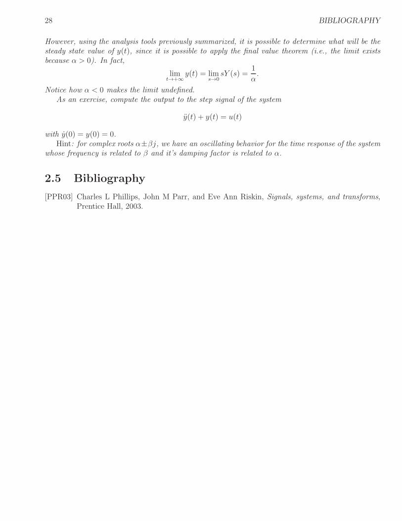
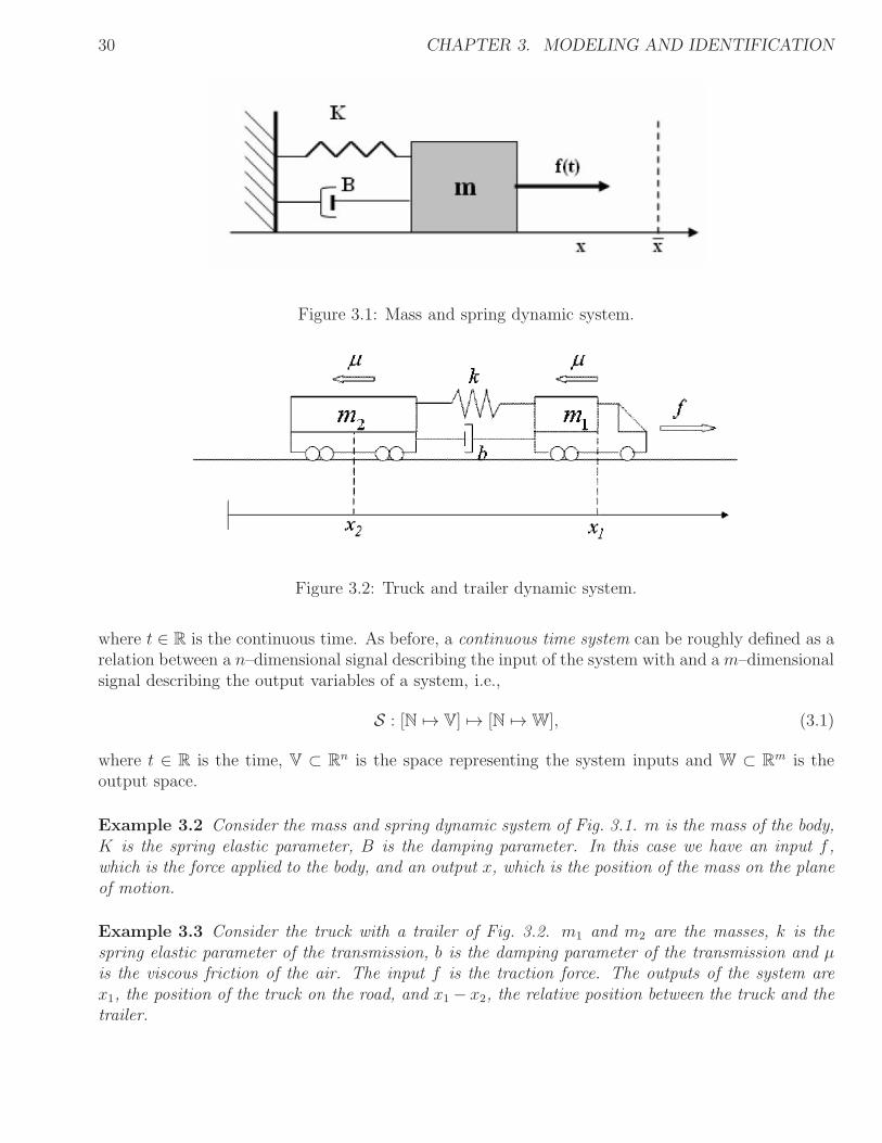
Example 3.2 Consider the mass and spring dynamic system of Fig. 3.1. m is the mass of the body,K is the spring elastic parameter, B is the damping parameter. In this case we have an input f ,which is the force applied to the body, and an output x, which is the position of the mass on the planeof motion.
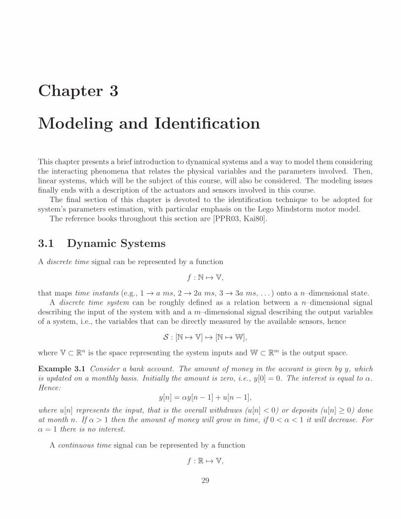
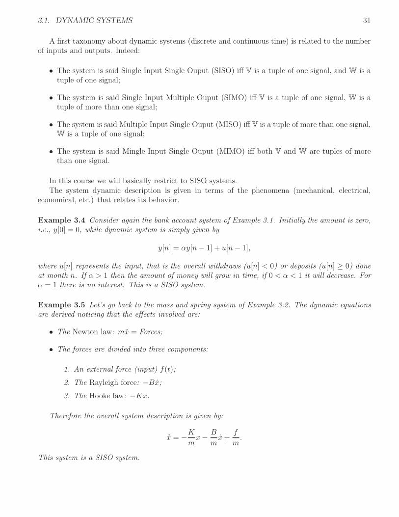
Example 3.3 Consider the truck with a trailer of Fig. 3.2. m1 and m2 are the masses, k is thespring elastic parameter of the transmission, b is the damping parameter of the transmission and µis the viscous friction of the air. The input f is the traction force. The outputs of the system arex1, the position of the truck on the road, and x1 − x2, the relative position between the truck and thetrailer.
3.1. DYNAMIC SYSTEMS 31
A first taxonomy about dynamic systems (discrete and continuous time) is related to the numberof inputs and outputs. Indeed:
• The system is said Single Input Single Ouput (SISO) iff V is a tuple of one signal, and W is atuple of one signal;
• The system is said Single Input Multiple Ouput (SIMO) iff V is a tuple of one signal, W is atuple of more than one signal;
• The system is said Multiple Input Single Ouput (MISO) iff V is a tuple of more than one signal,W is a tuple of one signal;
• The system is said Mingle Input Single Ouput (MIMO) iff both V and W are tuples of morethan one signal.
In this course we will basically restrict to SISO systems.The system dynamic description is given in terms of the phenomena (mechanical, electrical,
economical, etc.) that relates its behavior.
Example 3.4 Consider again the bank account system of Example 3.1. Initially the amount is zero,i.e., y[0] = 0, while dynamic system is simply given by
y[n] = αy[n− 1] + u[n− 1],
where u[n] represents the input, that is the overall withdraws (u[n] < 0) or deposits (u[n] ≥ 0) doneat month n. If α > 1 then the amount of money will grow in time, if 0 < α < 1 it will decrease. Forα = 1 there is no interest. This is a SISO system.
Example 3.5 Let’s go back to the mass and spring system of Example 3.2. The dynamic equationsare derived noticing that the effects involved are:
• The Newton law: mx = Forces;
• The forces are divided into three components:
1. An external force (input) f(t);
2. The Rayleigh force: −Bx;
3. The Hooke law: −Kx.
Therefore the overall system description is given by:
x = −Kmx− B
mx+
f
m.
This system is a SISO system.
32 CHAPTER 3. MODELING AND IDENTIFICATION
Example 3.6 For the truck and trailer system of Example 3.3. The dynamic equations are derivedfrom the Newton’s, Rayleigh’s and Hook’s laws, plus the aerodynamical drag force −µx2
i , with i = 1, 2.Therefore the overall system description is given by:
m1x1 = f − k(x1 − x2)− b(x1 − x2)− µx21
m2x2 = k(x1 − x2) + b(x1 − x2)− µx22
This system is a SIMO system.
In the rest of these notes, we will consider only one modeling technique, that is the I/O description.More in depth, we describe the possible behaviors of the system by showing how the output iscomputed directly from the input.
Continuous time systems are generically expressed by Ordinary Differential Equations (ODEs),while discrete time systems by difference equations. From the previous examples and by defining
D(k)x(t) =
x(t+ k)x(t) shifted forward by k time steps for difference equations,
dkx(t)
dtkthe k–th derivative of x(t) for continuous time,
,
we can infer that the I/O relation for a SISO system is in general given by
F(
y(t), D(1)y(t), . . . , D(n)y(t), u(t), D(1)u(t), . . . , D(p)u(t), t)
= 0,
where t ∈ R, y(t) : R 7→ R and u(t) : R 7→ R. If the system is well posed then it can be describedwith the normal form
D(n)y(t) = F(
y(t), D(1)y(t), . . . , D(n−1)y(t), u(t), D(1)u(t), . . . , D(p)u(t), t)
. (3.2)
A well posed system of difference or differential equations describes the whole time evolution ofthe involved physical quantities whenever the initial conditions are properly given. For a system innormal form (3.2), the initial conditions are specified by the values of y(t0) at time t0 (referred to asinitial time) and the corresponding values of all the n− 1 shift operators or time derivatives of y(t)at the same instant, together with u(t0) and the first p− 1 shift operators or time derivatives of u(t)at the same time instant.
Example 3.7 The discrete time equation in the Examples 3.4 and 3.5 are already in their normalform.
3.1.1 Fundamental Properties of Dynamic Systems
Dynamic systems may or may not satisfy a set of properties that can simplify their analysis andcontrol. Here in the following, the most important are presented and discussed.
Definition 3.8 (Causality) A system is causal if the output y(t) at time t is only related to theinitial conditions and from the inputs u(τ), for τ ≤ t. It is strictly causal if this relation is true forτ < t.
3.1. DYNAMIC SYSTEMS 33
In plain words, the “causal” adjective refers to the existence of a cause/effect relation betweeninputs and outputs. Therefore, a causal system cannot predict the future to produce its output, soall physical systems are causal. Examples of algorithmic exceptions: CD drive, media players andideal filters. In such cases, the output depends on the future inputs since the output is delayed.
Given a system expressed in normal form (3.2) is causal if p = n and strictly causal if p < n.
Definition 3.9 (Stationarity) If the system does not changes its behavior in time, it is time in-variant or stationary.
A system is stationary in its normal form (3.2) if dF (·)dt
= 0. The solution of a time invariantsystem does not changes if the initial time changes.
Definition 3.10 (Linearity) According to definition in (3.1), a system is linear if:
• Superposition principle: For any two inputs f(t) and g(t), the output of the system is
S(f + g)(t) = S(f)(t) + S(g)(t);
• Scaling: for any input f(t) and for any scalar α, the output of the system is
S(αf)(t) = αS(f)(t).
If the normal form (3.2) is given, a system is linear if it can be rewritten with
D(n)y(t) =n−1∑
i=0
ai(t)D(i)y(t) +
p∑
j=0
bj(t)D(j)u(t)
If it is also stationary, the terms ai and bj are constant. It comes out that for a linear systemthe analysis is rather simplified, since it is possible to apply the superposition principle and tocompute the trajectory in the state space by summation of a homogeneous solution and a genericsolution. This two solutions are referred to as the unforced system response (for u ≡ 0 and giveninitial conditions) and the forced response (for zero initial conditions and generic input). The forcedresponse is sometimes called the zero-state response to highlight the fact that the initial conditionsare zeroed.
Example 3.11 The bank account in Example 3.4 is a discrete-time causal, stationary and linearsystem. However, if the Examples 3.4 bank interest is supposed to change in time, the system be-comes non-stationary. The mass and spring system in Example 3.5 is a continuous time causal,stationary and linear system, while the truck and trailer of Example 3.6 is a continuous time causaland stationary system, however it is not linear.
34 CHAPTER 3. MODELING AND IDENTIFICATION
3.1.2 Impulse Response
The output response of a linear system subjected of a certain input is given by the convolutionbetween the impulse response (either h[n] for discrete time systems or h(t) for continuous time) ofthe system and the input, i.e.,
y[n] = h[n] ∗ u[n] or y(t) = h(t) ∗ u(t).
In the domain of the complex variable s, the previous convolution operation for continuous timesystems (which are the systems we will face during this course) turns to an algebraic operation forthe L-transform, i.e.,
Y (s) = H(s)U(s) +H0(s),
where H(s) is the transfer function of the system, that is by definition the L-transform of the impulseresponse of the system assuming zero–state initial condition, and H0(s) is the transfer function giventhe initial conditions. It turns then out that the inverse Laplace transform of H(s)U(s) is the forcedresponse of the system, while the inverse Laplace transform H0(s) is the unforced response. Forexample, these two components are clearly reported in Example 2.10.
3.2 Analysis of a Linear System
The analysis of the transfer function H(s) of a system dives a lot of information to the controlengineering on both the foreseen behavior of the system when it is subjected to nominal inputs, e.g.,impulse, unitary step, ramp, and the best way to control it and to modify its behavior. Usually, theanalysis is conducted by imposing as input the unitary step. This is mainly due by the simplicity ofthe input signal and, on the other hand, by the fact that a generic signal can be approximated witha piecewise constant signal.
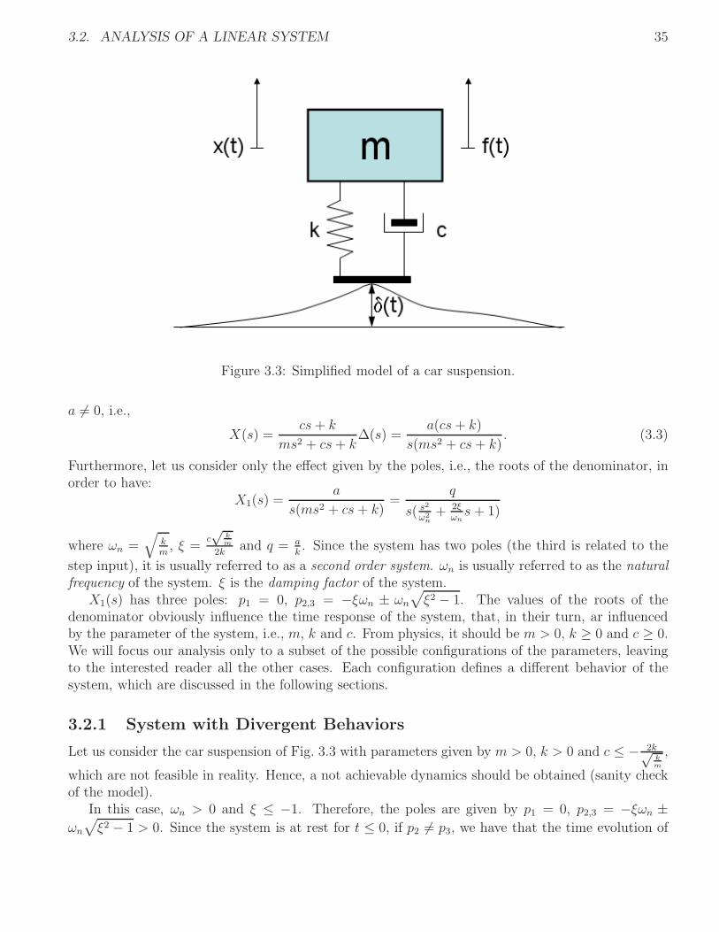
The analysis of a linear system is here proposed by using the practical example of a simplified carsuspension, reported in Fig. 3.3, which assumes the validity of the so–called quarter model of the car.m is one fourth of the total mass of the car, k is the spring elastic parameter of the suspension, whilec is the damping parameter of the suspension. δ(t) is the shape of the road (exogenous disturbanceinput) while f(t) is an external force applied to the car (the input to the model). x(t) is the positionof the vehicle, measure w.r.t. the vertical axis (system output).
Following the modeling procedure used in Examples 3.2 and 3.3, the dynamic model of the systemis
mx(t) + k(x(t)− δ(t)) + c(x(t)− δ(t)) = f(t)
where f(t) comprises also the force due to the gravity acceleration. Assuming that the system is atrest for t < 0, i.e., x(t) = x(t) = δ(t) = 0, ∀t < 0, the monolateral L trasform is given by
X(s)(ms2 + cs+ k) = F (s) + (cs+ k)∆(s).
Hence:
X(s) =1
ms2 + cs+ kF (s) +
cs + k
ms2 + cs+ k∆(s).
Recalling that the overall time evolution is obtained using the superposition principle, let us firstconsider only the effect of the road (F (s) = 0), assuming the wheel is climbing a step of amplitude
3.2. ANALYSIS OF A LINEAR SYSTEM 35
Figure 3.3: Simplified model of a car suspension.
a 6= 0, i.e.,
X(s) =cs+ k
ms2 + cs+ k∆(s) =
a(cs+ k)
s(ms2 + cs+ k). (3.3)
Furthermore, let us consider only the effect given by the poles, i.e., the roots of the denominator, inorder to have:
X1(s) =a
s(ms2 + cs+ k)=
q
s( s2
ω2n+ 2ξ
ωns + 1)
where ωn =√
km, ξ =
c√
km
2kand q = a
k. Since the system has two poles (the third is related to the
step input), it is usually referred to as a second order system. ωn is usually referred to as the naturalfrequency of the system. ξ is the damping factor of the system.
X1(s) has three poles: p1 = 0, p2,3 = −ξωn ± ωn
√
ξ2 − 1. The values of the roots of thedenominator obviously influence the time response of the system, that, in their turn, ar influencedby the parameter of the system, i.e., m, k and c. From physics, it should be m > 0, k ≥ 0 and c ≥ 0.We will focus our analysis only to a subset of the possible configurations of the parameters, leavingto the interested reader all the other cases. Each configuration defines a different behavior of thesystem, which are discussed in the following sections.
3.2.1 System with Divergent Behaviors
Let us consider the car suspension of Fig. 3.3 with parameters given by m > 0, k > 0 and c ≤ − 2k√km
,
which are not feasible in reality. Hence, a not achievable dynamics should be obtained (sanity checkof the model).
In this case, ωn > 0 and ξ ≤ −1. Therefore, the poles are given by p1 = 0, p2,3 = −ξωn ±ωn
√
ξ2 − 1 > 0. Since the system is at rest for t ≤ 0, if p2 6= p3, we have that the time evolution of
36 CHAPTER 3. MODELING AND IDENTIFICATION
the system is only given by the forced response
X1(s) =q
s( s2
ω2n+ 2ξ
ωns+ 1)
=c1s+
c2s− p2
+c3
s− p3,
whose inverse Laplace transform has the coefficients
c1 = sX1(s)|s=0 = q,
c2 = (s− p2)X1(s)|s=p2 =qω2
n
p2(p2 − p3),
c3 = (s− p3)X1(s)|s=p3 = −qω2
n
p3(p2 − p3),
and hence the time dynamic
x1(t) =
[
q +qω2
n
p2 − p3
(
ep2t
p2− ep3t
p3
)]
1(t).
On the other hand, if p2 = p3 = ωn (with ξ = −1), we have
X1(s) =q
s( s2
ω2n+ 2ξ
ωns+ 1)
=c1s+
c(1)2
s− ωn
+c(2)2
(s− ωn)2,
with coefficients
c1 = sX1(s)|s=0 = q,
c(1)2 =
1
1!
d
ds
[
(s− ωn)2X1(s)
]
|s=ωn= −q,
c(2)2 = (s− ωn)
2X1(s)|s=ωn= qωn,
that yields to
x1(t) =[
q − q(1− ωnt)eωnt
]
1(t).
Regardless of the amplitude of the step a, the final value of x1(t) in both cases for ξ ≤ −1 is
limt→+∞
x1(t) = sign(a)∞,
In other words, once the car climbs an unitary step, the car explodes! A realistic behavior would notbe the one here described, as it was supposed to be using a damping parameter c < 0 that, instead,generates energy! Notice that this is true even if −1 < ξ < 0 (that corresponds again to c < 0, butwith complex conjugated poles with positive real parts). In this case the limit is not defined, due tothe persistent and divergent oscillations.
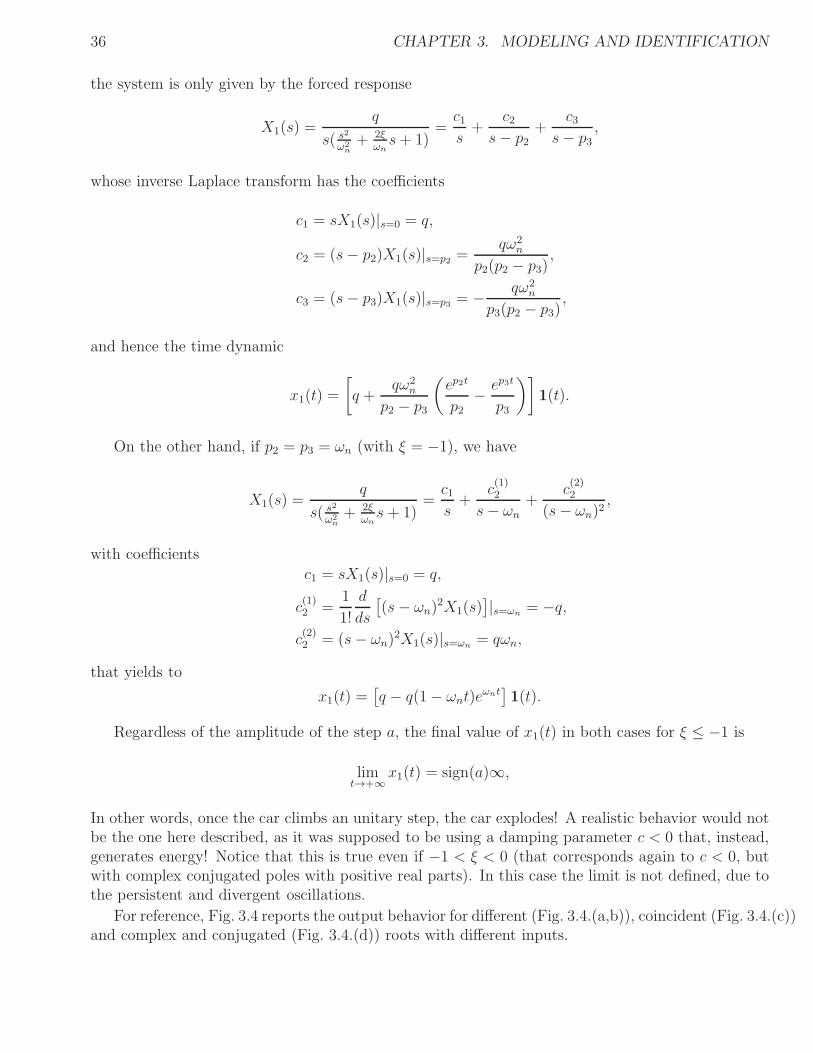
For reference, Fig. 3.4 reports the output behavior for different (Fig. 3.4.(a,b)), coincident (Fig. 3.4.(c))and complex and conjugated (Fig. 3.4.(d)) roots with different inputs.
3.2. ANALYSIS OF A LINEAR SYSTEM 37
0 1 2 3 4 5 6 7 8 9 100
10
20
30
40
50
60
70
80
90a = 0.1; k = 100; m = 400; c = −600
Time (sec)
Am
plit
ude
0 1 2 3 4 5 6 7 8 9 10−90
−80
−70
−60
−50
−40
−30
−20
−10
0a = −0.1; k = 100; m = 400; c = −600
Time (sec)
Am
plit
ude
(a) (b)
0 1 2 3 4 5 6 7 8 9 100
0.1
0.2
0.3
0.4
0.5
0.6
0.7a = 0.1; k = 100; m = 400; c = −400
Time (sec)
Am
plit
ude
0 5 10 15 20 25 30−1.6
−1.4
−1.2
−1
−0.8
−0.6
−0.4
−0.2
0
0.2
0.4a = 0.1; k = 100; m = 400; c = −200
Time (sec)
Am
plit
ude
(c) (d)
Figure 3.4: Divergent outputs due to: (a) Positive step a = 0.1, positive roots (ξ < −1), (b) Negativestep a = −0.1, positive roots (ξ < −1), (c) Positive step a = 0.1, positive coincident roots (ξ = −1),(d) Positive step a = 0.1, complex roots with positive real part (−1 < ξ < 0).
3.2.2 First Order Systems
Let us consider the car suspension of Fig. 3.3 with parameters given by m > 0, k > 0 and c ≥ 2k√km
,
a feasible dynamic. In this case, ωn > 0 and ξ ≥ 1. The poles are real and given by p1 = 0,p2,3 = −ξωn ± ωn
√
ξ2 − 1 < 0. Since the system is at rest for t ≤ 0, if p2 6= p3, we have that thetime evolution of the system is only given by the forced response
X1(s) =q
s( s2
ω2n+ 2ξ
ωns + 1)
=c1s+
c2s− p2
+c3
s− p3,
that, as done in Section 3.2.1, the time evolution is given by
x1(t) =
[
q +qω2
n
p2 − p3
(
ep2t
p2− ep3t
p3
)]
1(t).
In the case of coincident roots p2 = p3 = ωn (with ξ = 1), we have
x1(t) =[
q − q(1 + ωnt)e−ωnt
]
1(t).
38 CHAPTER 3. MODELING AND IDENTIFICATION
0 5 10 15 20 25 300
0.1
0.2
0.3
0.4
0.5
0.6
0.7
0.8
0.9
1x 10
−3
a = 0.25; k = 100; m = 400; c = 600
Time (sec)
Am
plit
ude
0 5 10 15 20 25 30−8
−7
−6
−5
−4
−3
−2
−1
0x 10
−4
a = −0.1; k = 100; m = 400; c = 2400
Time (sec)
Am
plit
ude
(a) (b)
0 5 10 15 20 25 300
0.1
0.2
0.3
0.4
0.5
0.6
0.7
0.8
0.9
1x 10
−3
a = 0.1; k = 100; m = 400; c = 400
Time (sec)
Am
plit
ude
(c)
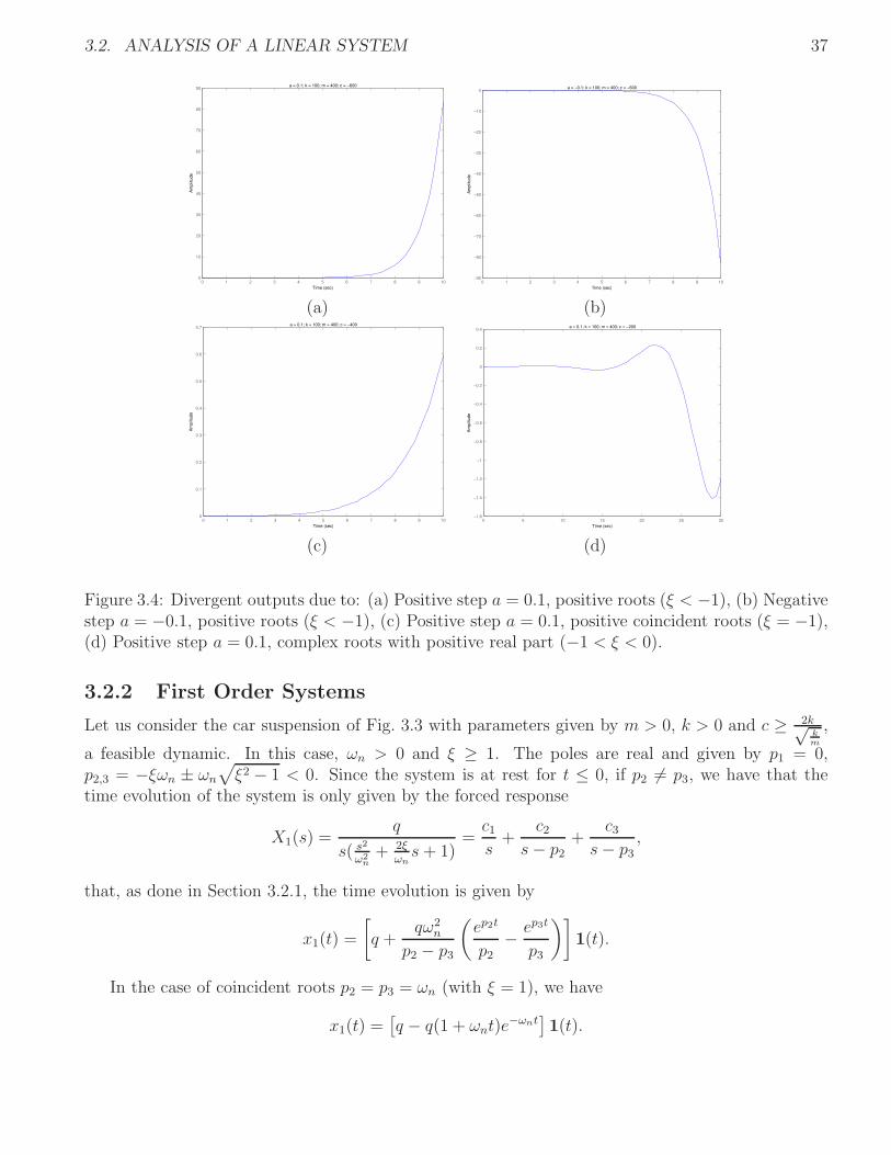
Figure 3.5: Convergent outputs due to: (a) Positive step a = 0.1, negative roots (ξ ≥ 1), (b) Negativestep a = −0.1, negative roots (ξ ≥ 1), (c) Positive step a = 0.1, negative coincident roots (ξ = 1).
The final value of x1(t) for ξ > 1 is
limt→+∞
x1(t) = q =a
k
or, equivalently (since the system has negative poles)
lims→0
sX1(s) =qω2
n
p2p3= q =
a
k.
The final value of x1(t) for ξ = 1 is
limt→+∞
x1(t) = q =a
kor lim
s→0sX1(s) =
qω2n
p22= q =
a
k
Again, Fig. 3.5 reports the output behavior for different (Fig. 3.5.(a,b)) and coincident (Fig. 3.5.(c))roots with different inputs.
An important characteristic of the output of a (stable) linear system, in addition to the steadystate value, is the time in which the system reaches that value. For this reason, this time is referred
3.2. ANALYSIS OF A LINEAR SYSTEM 39
to as the settling time Ts of the system. For engineers, it is not relevant when the system effectivelyreaches the steady state value (in fact, by the inverse Laplace transform, it is reached for t→ +∞),but it is more important the time in which the system reaches the α% of the steady state value andremains, for t → +∞, within that bound. This quantity is a function of the parameters ωn and ξof the system. Such a function is described by means of the time evolution of the system response.More precisely:
|q − x1(t)| ≤(
100− α
100
)
q = βq, ∀t ≥ Ts
Therefore, for ξ ≥ 1, p2 6= p3 and p2, p3 ∈ R−,
x1(t) =
[
q +qω2
n
p2 − p3
(
ep2t
p2− ep3t
p3
)]
1(t),
and, for a > 0 (q > 0) and t > 0,
|q − x1(t)| ≤ βq ⇒∣
∣
∣
∣
− qω2n
p2 − p3
(
ep2t
p2− ep3t
p3
)∣
∣
∣
∣
≤ βq.
Using the superposition principle, we have
epit ≤ β|pi(p2 − p3)|
ω2n
, for i = 2, 3,
that, using the logarithms we have
pit ≤ log(β|pi(p2 − p3)|)− log(ω2n),
and, finally
Ts =log(β|pi(p2 − p3)|)− log(ω2
n)
pi.
Hence for each root, we have two possible values for the time Ts. Of course, the root that issmaller in modulus will govern the rate of convergence of the system towards its steady state value.This idea is quite effective from a practical view–point and it can be generalized to any numberof roots, even if the roots are complex. This approximation is usually referred to as the systemapproximation of the dominant pole. Fig. 3.6.(a) depicts the approximation to the dominant polethus introduced for this system. For the described system, assuming that p2 = −ξωn + ωn
√
ξ2 − 1
and p3 = −ξωn − ωn
√
ξ2 − 1, p2 is the dominant pole. Hence, the greater (in modulus) is p2, the
faster is the rate of convergence. This result is accomplished by increasing ωn =√
km
and making
ξ =c√
km
2k→ 1. Fig. 3.6.(b) reports the output for two different choices of the spring constant with
a mass m = 400 kg.If p2 = p3 = ωn (with ξ = 1), we have
x1(t) =[
q − q(1 + ωnt)e−ωnt
]
1(t),
hence|q − x1(t)| ≤ βq ⇒ |q(1 + ωnt)e
−ωnt| ≤ βq.
40 CHAPTER 3. MODELING AND IDENTIFICATION
0 5 10 15 20 25 300
0.001
0.002
0.003
0.004
0.005
0.006
0.007
0.008
0.009
0.01G2
Time (sec)
Am
plit
ud
e
x1(t)
only p2
only p3
0 5 10 15 20 25 300
0.1
0.2
0.3
0.4
0.5
0.6
0.7
0.8
0.9
1x 10
−3
Comparison
Time (sec)
Am
plit
ud
e
Choice 1
Choice 2
(a) (b)
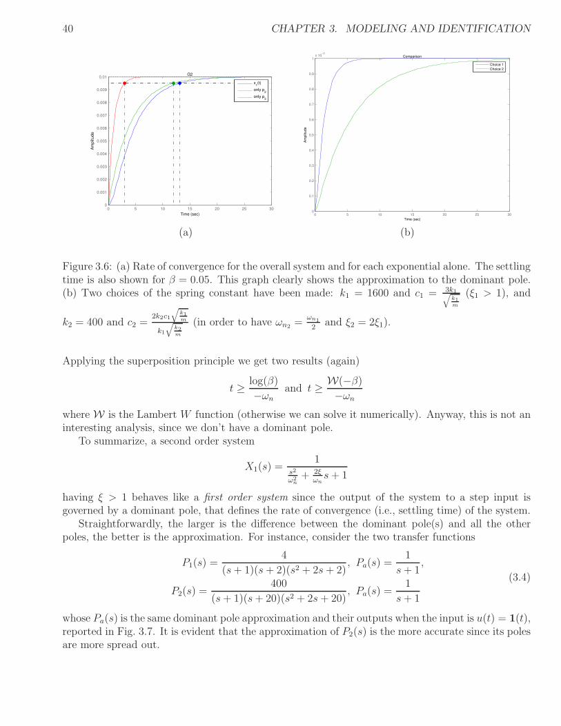
Figure 3.6: (a) Rate of convergence for the overall system and for each exponential alone. The settlingtime is also shown for β = 0.05. This graph clearly shows the approximation to the dominant pole.(b) Two choices of the spring constant have been made: k1 = 1600 and c1 = 3k1
√
k1m
(ξ1 > 1), and
k2 = 400 and c2 =2k2c1
√
k1m
k1
√
k2m
(in order to have ωn2=
ωn1
2and ξ2 = 2ξ1).
Applying the superposition principle we get two results (again)
t ≥ log(β)
−ωn
and t ≥ W(−β)−ωn
where W is the Lambert W function (otherwise we can solve it numerically). Anyway, this is not aninteresting analysis, since we don’t have a dominant pole.
To summarize, a second order system
X1(s) =1
s2
ω2n+ 2ξ
ωns+ 1
having ξ > 1 behaves like a first order system since the output of the system to a step input isgoverned by a dominant pole, that defines the rate of convergence (i.e., settling time) of the system.
Straightforwardly, the larger is the difference between the dominant pole(s) and all the otherpoles, the better is the approximation. For instance, consider the two transfer functions
P1(s) =4
(s+ 1)(s+ 2)(s2 + 2s+ 2), Pa(s) =
1
s+ 1,
P2(s) =400
(s+ 1)(s+ 20)(s2 + 2s+ 20), Pa(s) =
1
s+ 1
(3.4)
whose Pa(s) is the same dominant pole approximation and their outputs when the input is u(t) = 1(t),reported in Fig. 3.7. It is evident that the approximation of P2(s) is the more accurate since its polesare more spread out.

3.2. ANALYSIS OF A LINEAR SYSTEM 41
0 1 2 3 4 5 6 7 8
0.0
0.1
0.2
0.3
0.4
0.5
0.6
0.7
0.8
0.9
1.0
P_1
P_2
P_a
P_1
P_2
P_a
Figure 3.7: Response to a unitary input for the plants reported in eqrefeq:AnalysisDomPoles whosedominant pole approximation is given by the same Pa(s).
3.2.3 Second Order Systems
Let us consider the car suspension of Fig. 3.3 with parameters given bym > 0, k > 0 and 0 < c ≤ 2k√km
.
In this case, ωn > 0 and 0 < ξ < 1. The poles are then complex and conjugated and given by p1 = 0,p2,3 = −ξωn ± jωn
√
1− ξ2, with negative real part. xSince the system is at rest for t ≤ 0, we havethat the time evolution of the system is only given by the forced response is
X1(s) =q
s( s2
ω2n+ 2ξ
ωns + 1)
=c1s+
c2s− p2
+c3
s− p3,
with coefficients given by
c1 = sX1(s)|s=0 = q,
c2 = (s− p2)X1(s)|s=p2 =qω2
n
p2(p2 − p3)=−√
1− ξ2 − ξj
2√
1− ξ2,
c3 = (s− p3)X1(s)|s=p3 = −qω2
n
p3(p2 − p3)=−√
1− ξ2 + ξj
2√
1− ξ2,
which yields to the time response
x1(t) =[
q + 2Ne−ξωnt cos(ωn
√
1− ξ2t+ φ)]
1(t)

42 CHAPTER 3. MODELING AND IDENTIFICATION
with N = q
2√
1−ξ2and φ = arctan
(
ξ
−√
1−ξ2
)
.
Noticing that:
1. cos(θ) = − sin(
θ − π2
)
;
2. arctan(
sin(θ)cos(θ)
)
− π2= arctan
(
− cos(θ)sin(θ)
)
;
It follows thatx1(t) =
[
q − qNe−ξωnt sin(ωn
√
1− ξ2t+ φ)]
1(t),
with N = 1√1−ξ2
and φ = arctan
(√1−ξ2
ξ
)
. The final value of x1(t) for 0 < ξ < 1 is again
limt→+∞
x1(t) = q =a
k
Let us now consider the settling time in this particular case. Again
|q − x1(t)| ≤ βq, ∀t ≥ Ts,
or, equivalently,|Ne−ξωnt sin(ωn
√
1− ξ2t+ φ)| ≤ β.
Due to the sinusoidal function, this equation is quite difficult to evaluate. An effective upper boundto Ts is derived using a worst case approach, i.e., by considering | sin(ωn
√
1− ξ2t + φ)| = 1, andrecalling that N > 0 for 0 < ξ < 1, i.e.,
e−ξωnt ≤ β
N,
and finally get
Ts ≈log(β)− log(N)
−ξωn
.
Notice that the real part of the complex roots −ξωn plays a fundamental role in rate of convergencetowards the steady state value.
Another important parameter for a second order system is given by the overshoot, that is themaximum value reached by the time evolution of the output with respect to the steady state value.More precisely, the overshoot O is defined as the difference between the maximum value reached bythe system response xmax and the steady state value x(∞), normalized by the difference between theinitial value x(0) and the steady state value
O =|xmax − x(∞)||x(0)− x(∞)| .
An exact relation between the damping parameter ξ and the overshoot O is derived computing thetime derivative
dx1(t)
dt= −qNe−ξωntωn
√
1− ξ2 cos(ωn
√
1− ξ2t+ φ)
+ qξωnNe−ξωnt sin(ωn
√
1− ξ2t+ φ) =
− ωn
√
1− ξ2 cos(ωn
√
1− ξ2t+ φ) + ξωn sin(ωn
√
1− ξ2t + φ),
3.2. ANALYSIS OF A LINEAR SYSTEM 43
and imposing it to be equal to 0, which yields to
tan(
ωn
√
1− ξ2t+ φ)
=
√
1− ξ2
ξ.
Recalling that tan(φ) =
√1−ξ2
ξ, it follows that ωn
√
1− ξ2t = hπ, with h = 0, 1, . . . . Hence the
maximum and minimum values for x1(t) are given by the time instants
th =hπ
ωn
√
1− ξ2,
relation that highlights the dependence of the step response to the imaginary part of the complexroot. Rewriting the time evolution of the system response using these derived relations
x1(t) = q
1− e− hπξ√
1−ξ2
√
1− ξ2sin(hπ + φ)
,
and noticing thatsin(hπ + φ) = sin(φ) cos(hπ) = sin(φ)(−1)h,
and
tan(φ) =
√
1− ξ2
ξ⇒ sin(φ) =
√
1− ξ2,
we finally get to
x1(t) = q
[
1− (−1)he−hπξ√1−ξ2
]
.
It is now evident that for h = 1 we have a maximum. Hence, the time in which the system reachesits maximum value is
To =π
ωn
√
1− ξ2.
Increasing ωn, the overshoot will happen earlier. On the other hand, it will happen later if ξincreases. The corresponding overshoot value is obtained noticing that x(0) = 0, x(∞) = q and
xmax = q
[
1 + e− πξ√
1−ξ2
]
.
Therefore
O =|xmax − x(∞)||x(0)− x(∞)| = e
− πξ√1−ξ2 ,
i.e., the maximum overshoot depends only on the damping parameter ξ of the complex roots. Forexample, if a maximum overshoot is desired, ξ should be greater than a ξmin.
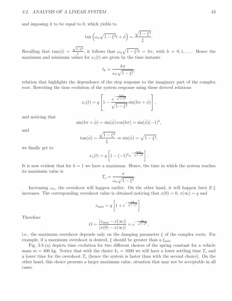
Fig. 3.8.(a) depicts time evolution for two different choices of the spring constant for a vehiclemass m = 400 kg. Notice that with the choice k1 = 1600 we will have a lower settling time Ts anda lower time for the overshoot To (hence the system is faster than with the second choice). On theother hand, this choice presents a larger maximum value, situation that may not be acceptable in allcases.

44 CHAPTER 3. MODELING AND IDENTIFICATION
0 5 10 150
0.5
1
1.5x 10
−3
Comparison
Time (sec)
Am
plit
ud
e
Choice 1
Choice 2
0 5 10 15 20 25 300
0.2
0.4
0.6
0.8
1
1.2
1.4
1.6
1.8
2x 10
−3
a = 0.1; k = 100; m = 400; c = 0
Time (sec)
Am
plit
ud
e
(a) (b)
Figure 3.8: (a) Two choices of the spring constant have been made: k1 = 1600 and c1 = k1
2√
k1m
(0 < ξ1 < 1), and k2 = 400 and c2 =2k2c1
√
k1m
k1
√
k2m
(in order to have ωn2=
ωn1
2and ξ2 = 2ξ1 < 1). The
settling time is referred to a threshold of β = 0.02. (b) Imaginary roots.
With a different choice of the parameters, the output can be completely different (Fig. 3.8.(b)).Indeed, in the case of m > 0, k > 0 and c = 0, the oscillations are not dumped since the transferfunction has p1 = 0 and p2,3 that are complex and conjugated with Re(p2,3) = 0. In this case, it isnot possible to define the Ts, but it is possible to define the overshoot (left as exercise).
Let us now recall the overall transfer function (3.3) given by the effect of the road (F (s) = 0)and the road, i.e.,
X(s) = (cs+ k)X1(s),
In this case, the real system response is given by the previously obtained time evolution (multipliedby k) with added the time derivative of the time response x1(t), scaled by the factor c, i.e.,
x(t) = cdx1(t)
dt+ kx1(t).
Notice how a zero pops up in this case. To analyze how this zero modifies the output of the system,let us consider a generic second order system with stable, complex and conjugated roots (0 < ξ < 1,ωn > 0)
Y (s) =τs+ 1
s( s2
ω2n+ 2ξ
ωns+ 1)
= (τs+ 1)G(s),
excited by an unitary step signal. Define y1(t) = L−1[G(s)]. Therefore, y(t) = τ y1(t)dt
+ y1(t). Hence:
y(t) =− τβNe−ξωnt cos(βt+ φ) + τNξωne−ξωnt sin(βt+ φ)
+ 1− Ne−ξωnt sin(βt+ φ),
3.2. ANALYSIS OF A LINEAR SYSTEM 45
0 2 4 6 8 10−4
−2
0
2
4
6
8Comparison
sec
y(t
)
τ = 0
τ = 1
τ = 1.2
τ = −1
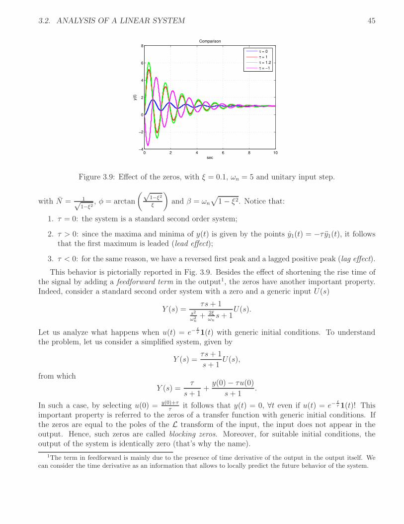
Figure 3.9: Effect of the zeros, with ξ = 0.1, ωn = 5 and unitary input step.
with N = 1√1−ξ2
, φ = arctan
(√1−ξ2
ξ
)
and β = ωn
√
1− ξ2. Notice that:
1. τ = 0: the system is a standard second order system;
2. τ > 0: since the maxima and minima of y(t) is given by the points y1(t) = −τ y1(t), it followsthat the first maximum is leaded (lead effect);
3. τ < 0: for the same reason, we have a reversed first peak and a lagged positive peak (lag effect).
This behavior is pictorially reported in Fig. 3.9. Besides the effect of shortening the rise time ofthe signal by adding a feedforward term in the output1, the zeros have another important property.Indeed, consider a standard second order system with a zero and a generic input U(s)
Y (s) =τs+ 1
s2
ω2n+ 2ξ
ωns+ 1
U(s).
Let us analyze what happens when u(t) = e−tτ 1(t) with generic initial conditions. To understand
the problem, let us consider a simplified system, given by
Y (s) =τs+ 1
s+ 1U(s),
from which
Y (s) =τ
s+ 1+
y(0)− τu(0)
s+ 1.
In such a case, by selecting u(0) = y(0)+τ
τit follows that y(t) = 0, ∀t even if u(t) = e−
tτ 1(t)! This
important property is referred to the zeros of a transfer function with generic initial conditions. Ifthe zeros are equal to the poles of the L transform of the input, the input does not appear in theoutput. Hence, such zeros are called blocking zeros. Moreover, for suitable initial conditions, theoutput of the system is identically zero (that’s why the name).
1The term in feedforward is mainly due to the presence of time derivative of the output in the output itself. We
can consider the time derivative as an information that allows to locally predict the future behavior of the system.
46 CHAPTER 3. MODELING AND IDENTIFICATION
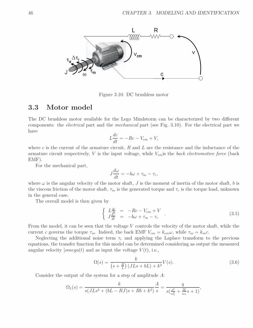
Figure 3.10: DC brushless motor
3.3 Motor model
The DC brushless motor available for the Lego Mindstorm can be characterized by two differentcomponents: the electrical part and the mechanical part (see Fig. 3.10). For the electrical part wehave
Ldc
dt= −Rc− Vcm + V,
where c is the current of the armature circuit, R and L are the resistance and the inductance of thearmature circuit respectively, V is the input voltage, while Vcmis the back electromotive force (backEMF).
For the mechanical part,
Jdω
dt= −bω + τm − τr,
where ω is the angular velocity of the motor shaft, J is the moment of inertia of the motor shaft, b isthe viscous friction of the motor shaft, τm is the generated torque and τr is the torque load, unknownin the general case.
The overall model is then given by
Ldcdt
= −Rc− Vcm + VJ dω
dt= −bω + τm − τr
. (3.5)
From the model, it can be seen that the voltage V controls the velocity of the motor shaft, while thecurrent c governs the torque τm. Indeed, the back EMF Vcm = kcmω, while τm = kmc.
Neglecting the additional noise term τr and applying the Laplace transform to the previousequations, the transfer function for this model can be determined considering as output the measuredangular velocity ]omega(t) and as input the voltage V (t), i.e.,
Ω(s) =k
(
s+ RL
)
(JLs + bL) + k2V (s). (3.6)
Consider the output of the system for a step of amplitude A:
Ω1(s) =k
s(JLs2 + (bL− RJ)s+Rb+ k2)
A
s=
q
s( s2
ω2n+ 2ξ
ωns+ 1)
,
3.4. IDENTIFICATION 47
where ωn =√
Rb+k2
JL, ξ =
√
Rb+k2
JL(bL−RJ)
2(Rb+k2)and q = kA
Rb+k2. Since the system has two poles (the third is
related to the step input), it is a second order system. Therefore, its output can be analyzed withthe tools introduced in Section 3.2.3.
3.4 Identification
System identification is a general term to describe mathematical tools and algorithms that builddynamical models from measured data. Measured data are used to calculate a transfer function ofthe system. Two different approaches are usually adopted for linear systems:
1. Time–domain approach: A measure of the time response of a system can be derived using acontrolled input.
2. Frequency–domain approach: A measure of the frequency response of a stable system can bederived using a sinusoidal input. Those measurements can be used to produce a Bode’ plot ofthe frequency response.
3.4.1 Time Domain Approach
A common approach is to start from the behavior of the system (known by the measured outputsof the system) and the known external influences (inputs to the system) and try to determine amathematical relation between them without going into the details of what is actually happeninginside the system. This approach is called system identification. Two types of models are commonin the field of system identification:
1. black box model: no prior model is available. Most system identification algorithms are of thistype;
2. grey box model: a certain model based on both insight into the system and experimental data isconstructed. This model does however still have a number of unknown free parameters whichcan be estimated using system identification.
In these notes the objective of system identification are the Lego motor parameters. We alreadyknow that a system like that acts as a second order system. As a consequence, we adopt the greybox model.
All the identification procedures need some measured data to extrapolate the model and someother to validate the identified model. In plain words, to identify the parameters of a model we needto check if a model fits experimental measurements or other empirical data. A common approach totest this fit is to split the data into two disjoint subsets:
1. Training data: are used to estimate the model parameters;
2. Verification data: are used to test the model. An accurate model will closely match theverification data even though this data was not used to set the model’s parameters (cross-validation).

48 CHAPTER 3. MODELING AND IDENTIFICATION
The second procedure is called model verification. A metric is needed to measure distancesbetween observed ym(t) and predicted data y(t) and, hence, to assess model fit. As a metric, we canadopt some standard indices used as performance indices for control systems:
• Integral squared error (ISE) =∫ T
0(ym(t)− y(t))2dt;
• Integral absolute error (IAE) =∫ T
0|ym(t)− y(t)|dt;
• Integral time squared error (ITSE) =∫ T
0t(ym(t)− y(t))2dt;
• Integral time absolute error (ITAE) =∫ T
0t|ym(t)− y(t)|dt.
A rigorous approach to system identification implies the adoption of the chosen metric as anobjective function to minimize in the procedure. For example, a technique usually adopted is the(linear) regression to gain the minimum mean squared error (MMSE). For our purposes and due tothe simplicity of the identification problem, we adopt a simpler trial–and–error procedure:
1. We collect output measurements and then we try to estimate second order system parameters(for instance, using a least square approach);
2. Next, we verify the estimated model against measurements, computing the fitting error usingthe chosen metric;
3. If the estimated values are satisfactory, then the procedure terminates, otherwise a differentchoice is made at point 1.
Example 3.12 Let us consider the motor model (3.6), shown in Fig. 3.10. Its time response is givenby:
ω1(t) =[
q + 2Ne−ξωnt cos(ωn
√
1− ξ2t+ φ)]
1(t)
with N = q
2√
1−ξ2and φ = arctan
(
ξ
−√
1−ξ2
)
. The final value of ω1(t) for 0 < ξ < 1 is
limt→+∞
ω1(t) = q,
the settling time (α is the percentage used to evaluate the settling time, while N = 1√1−ξ2
) is
Ts ≈log
(
α100
)
− log(N)
−ξωn
,
and finally the overshoot is given by
O =|ω
max− ω(∞)|
|ω(0)− ω(∞)| = e− πξ√
1−ξ2
The relation involving the settling time is approximated. As a consequence, the estimates of ωn
derived from that equation can be very inaccurate. In combination with the settling time, we can use
3.4. IDENTIFICATION 49
the real part of the complex and conjugated poles, that is −ξωn. In particular, the decay rate of theoscillations are given by e−ξωnt. Therefore,
loge−ξωn(t0+T )
e−ξωnt0= log
ω(t0 + T )− ω(∞)
ω(t0)− ω(∞),
where t0 is a certain time instant, while T is the period of the oscillations. For example, t0 can befixed as the time of one maximum of the oscillations (for instance, the overshoot), and t0 + T is thetime of the next maximum. However, the minima can also be chosen. It has to be noted that it ispossible to have more than one pair of measurements from the output signal. On the other hand, forhighly damped outputs it can be difficult to detect the output peaks, even though they exists.
Additionally, in order to have an estimate of ωn, we can exploit the relation of the oscillationfrequency, that is the imaginary part of the complex and conjugated roots, i.e.,
ωd = ωn
√
1− ξ2.
Therefore, by measuring the time between two consecutive peaks, the period T of the oscillations canbe derived. Hence,
ωn =2π
T√
1− ξ2.
Again, multiple estimates of the period are available.
3.4.2 Frequency Domain Approach
The rationale underlying the frequency domain approach is related to the harmonic response of alinear, open–loop asymptotically stable system described by G(jω). In such a case we already knowthat after the transient
u(t) = a sin(ωt)→ y(t) = |G(jω)|a sin(ωt+ ∠G(jω)),
and, using as inputs some sinusoids with different frequencies ω, we can get the frequency responseof the system approximated by points. From the frequency response, we get the transfer functiondescription. However, since we are using sampled data signals, attention must be payed to therelation of the frequency ω and the sampling time used for the output sampling, since aliasing effectsmay rise.
The gain is easily estimated by taking the ratio between the peaks of the input and those of theoutputs (that will happen, in general, at different times due to the presence of the phase ∠G(jω)).Therefore:
|G(jω)| = ymaxumax
,
while the phase is again estimated using the peak times ty and tu of the output and input signals,respectively. In particular, we have:
ωty + ∠G(jω) =π
2+ ky2π, and ωtu =
π
2+ ku2π.
where ku, ky ∈ Z. It has to be noted that in general ku 6= ky if the number of peaks for the outputand the input is not correctly taken into account. However this is not a problem as soon as we exploitthe grey–box approach to system identification, since the system is second order. Therefore:
∠G(jω) = ω(tu − ty) + (ky − ku)2π,

50 BIBLIOGRAPHY
but, since the phase is at most −π, we can simply limit the estimated ∠G(jω) ∈ [−2π, 0].
3.5 Bibliography
[Kai80] Thomas Kailath, Linear systems, vol. 1, Prentice-Hall Englewood Cliffs, NJ, 1980.
[PPR03] Charles L Phillips, John M Parr, and Eve Ann Riskin, Signals, systems, and transforms,Prentice Hall, 2003.
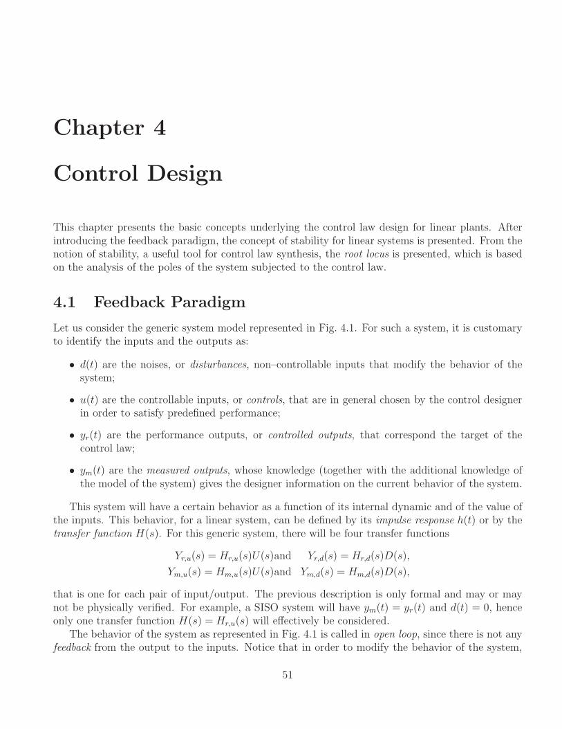
Chapter 4
Control Design
This chapter presents the basic concepts underlying the control law design for linear plants. Afterintroducing the feedback paradigm, the concept of stability for linear systems is presented. From thenotion of stability, a useful tool for control law synthesis, the root locus is presented, which is basedon the analysis of the poles of the system subjected to the control law.
4.1 Feedback Paradigm
Let us consider the generic system model represented in Fig. 4.1. For such a system, it is customaryto identify the inputs and the outputs as:
• d(t) are the noises, or disturbances, non–controllable inputs that modify the behavior of thesystem;
• u(t) are the controllable inputs, or controls, that are in general chosen by the control designerin order to satisfy predefined performance;
• yr(t) are the performance outputs, or controlled outputs, that correspond the target of thecontrol law;
• ym(t) are the measured outputs, whose knowledge (together with the additional knowledge ofthe model of the system) gives the designer information on the current behavior of the system.
This system will have a certain behavior as a function of its internal dynamic and of the value ofthe inputs. This behavior, for a linear system, can be defined by its impulse response h(t) or by thetransfer function H(s). For this generic system, there will be four transfer functions
Yr,u(s) = Hr,u(s)U(s)and Yr,d(s) = Hr,d(s)D(s),
Ym,u(s) = Hm,u(s)U(s)and Ym,d(s) = Hm,d(s)D(s),
that is one for each pair of input/output. The previous description is only formal and may or maynot be physically verified. For example, a SISO system will have ym(t) = yr(t) and d(t) = 0, henceonly one transfer function H(s) = Hr,u(s) will effectively be considered.
The behavior of the system as represented in Fig. 4.1 is called in open loop, since there is not anyfeedback from the output to the inputs. Notice that in order to modify the behavior of the system,
51
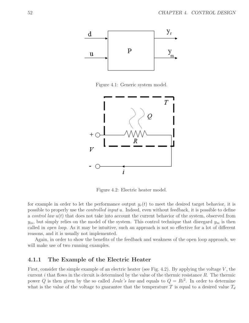
52 CHAPTER 4. CONTROL DESIGN
Figure 4.1: Generic system model.
Figure 4.2: Electric heater model.
for example in order to let the performance output yr(t) to meet the desired target behavior, it ispossible to properly use the controlled input u. Indeed, even without feedback, it is possible to definea control law u(t) that does not take into account the current behavior of the system, observed fromym, but simply relies on the model of the system. This control technique that disregard ym is thencalled in open loop. As it may be intuitive, such an approach is not so effective for a lot of differentreasons, and it is usually not implemented.
Again, in order to show the benefits of the feedback and weakness of the open loop approach, wewill make use of two running examples.
4.1.1 The Example of the Electric Heater
First, consider the simple example of an electric heater (see Fig. 4.2). By applying the voltage V , thecurrent i that flows in the circuit is determined by the value of the thermic resistance R. The thermicpower Q is then given by the so called Joule’s law and equals to Q = Ri2. In order to determinewhat is the value of the voltage to guarantee that the temperature T is equal to a desired value Td
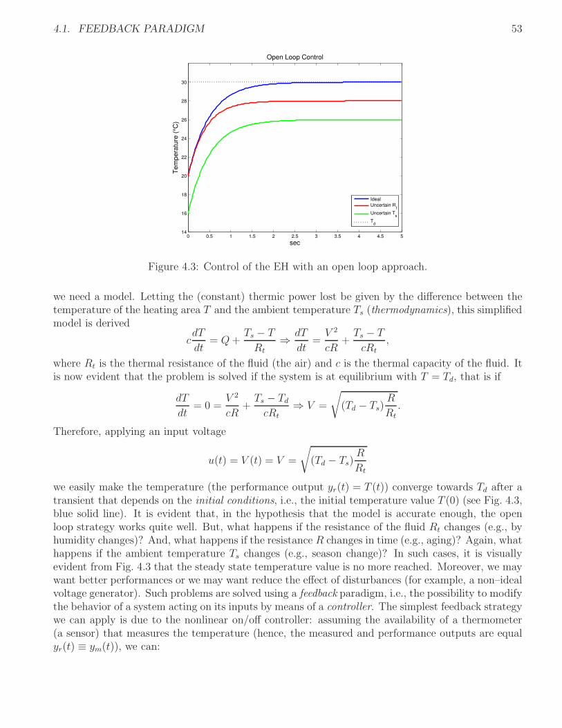
4.1. FEEDBACK PARADIGM 53
0 0.5 1 1.5 2 2.5 3 3.5 4 4.5 514
16
18
20
22
24
26
28
30
sec
Te
mp
era
ture
(°C
)
Open Loop Control
Ideal
Uncertain Rt
Uncertain Ts
Td
Figure 4.3: Control of the EH with an open loop approach.
we need a model. Letting the (constant) thermic power lost be given by the difference between thetemperature of the heating area T and the ambient temperature Ts (thermodynamics), this simplifiedmodel is derived
cdT
dt= Q+
Ts − T
Rt
⇒ dT
dt=
V 2
cR+
Ts − T
cRt
,
where Rt is the thermal resistance of the fluid (the air) and c is the thermal capacity of the fluid. Itis now evident that the problem is solved if the system is at equilibrium with T = Td, that is if
dT
dt= 0 =
V 2
cR+
Ts − Td
cRt
⇒ V =
√
(Td − Ts)R
Rt
.
Therefore, applying an input voltage
u(t) = V (t) = V =
√
(Td − Ts)R
Rt
we easily make the temperature (the performance output yr(t) = T (t)) converge towards Td after atransient that depends on the initial conditions, i.e., the initial temperature value T (0) (see Fig. 4.3,blue solid line). It is evident that, in the hypothesis that the model is accurate enough, the openloop strategy works quite well. But, what happens if the resistance of the fluid Rt changes (e.g., byhumidity changes)? And, what happens if the resistance R changes in time (e.g., aging)? Again, whathappens if the ambient temperature Ts changes (e.g., season change)? In such cases, it is visuallyevident from Fig. 4.3 that the steady state temperature value is no more reached. Moreover, we maywant better performances or we may want reduce the effect of disturbances (for example, a non–idealvoltage generator). Such problems are solved using a feedback paradigm, i.e., the possibility to modifythe behavior of a system acting on its inputs by means of a controller. The simplest feedback strategywe can apply is due to the nonlinear on/off controller: assuming the availability of a thermometer(a sensor) that measures the temperature (hence, the measured and performance outputs are equalyr(t) ≡ ym(t)), we can:
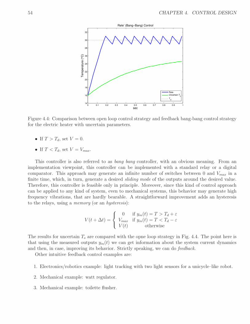
54 CHAPTER 4. CONTROL DESIGN
0 0.1 0.2 0.3 0.4 0.5 0.6 0.7 0.8 0.9 114
16
18
20
22
24
26
28
30
32
sec
Te
mp
era
ture
(°C
)
Rele’ (Bang−Bang) Control
Rele
Uncertain Ts
Td
Figure 4.4: Comparison between open loop control strategy and feedback bang-bang control strategyfor the electric heater with uncertain parameters.
• If T > Td, set V = 0.
• If T < Td, set V = Vmax.
This controller is also referred to as bang bang controller, with an obvious meaning. From animplementation viewpoint, this controller can be implemented with a standard relay or a digitalcomparator. This approach may generate an infinite number of switches between 0 and Vmax in afinite time, which, in turn, generate a desired sliding mode of the outputs around the desired value.Therefore, this controller is feasible only in principle. Moreover, since this kind of control approachcan be applied to any kind of system, even to mechanical systems, this behavior may generate highfrequency vibrations, that are hardly bearable. A straightforward improvement adds an hysteresisto the relays, using a memory (or an hysteresis):
V (t+∆t) =
0 if ym(t) = T > Td + εVmax if ym(t) = T < Td − εV (t) otherwise
The results for uncertain Ts are compared with the opne loop strategy in Fig. 4.4. The point here isthat using the measured outputs ym(t) we can get information about the system current dynamicsand then, in case, improving its behavior. Strictly speaking, we can do feedback.
Other intuitive feedback control examples are:
1. Electronics/robotics example: light tracking with two light sensors for a unicycle–like robot.
2. Mechanical example: watt regulator.
3. Mechanical example: toilette flusher.
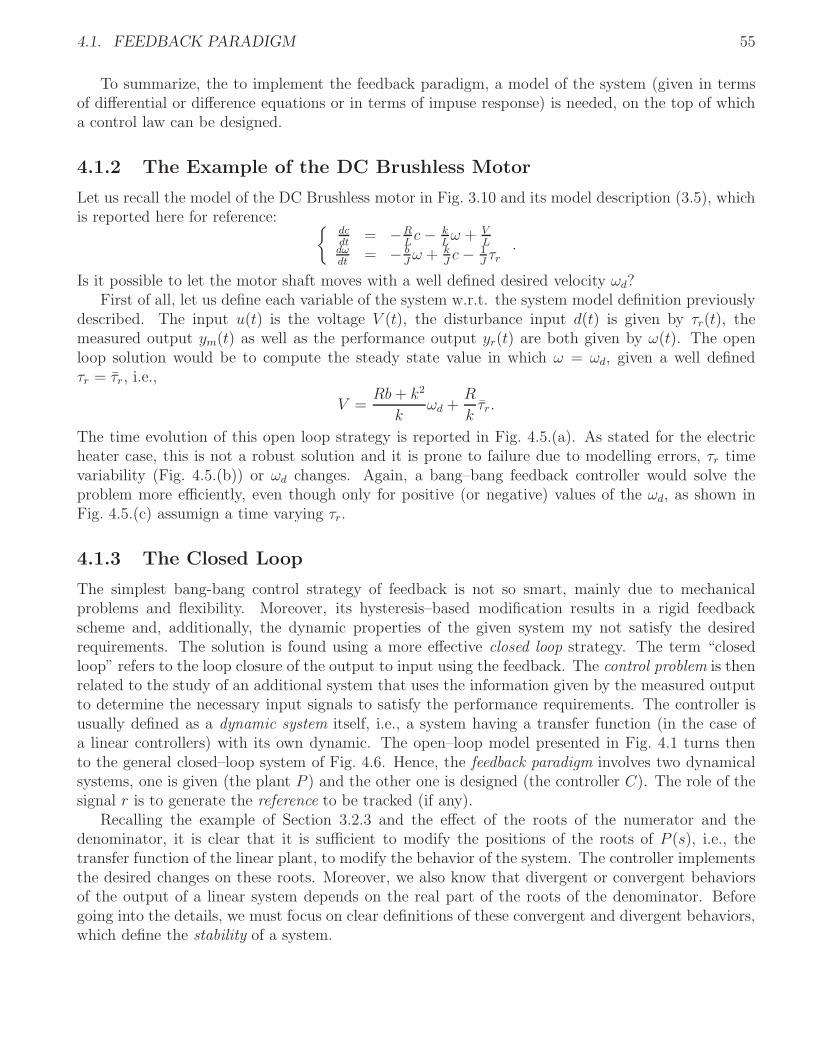
4.1. FEEDBACK PARADIGM 55
To summarize, the to implement the feedback paradigm, a model of the system (given in termsof differential or difference equations or in terms of impuse response) is needed, on the top of whicha control law can be designed.
4.1.2 The Example of the DC Brushless Motor
Let us recall the model of the DC Brushless motor in Fig. 3.10 and its model description (3.5), whichis reported here for reference:
dcdt
= −RLc− k
Lω + V
Ldωdt
= − bJω + k
Jc− 1
Jτr
.
Is it possible to let the motor shaft moves with a well defined desired velocity ωd?First of all, let us define each variable of the system w.r.t. the system model definition previously
described. The input u(t) is the voltage V (t), the disturbance input d(t) is given by τr(t), themeasured output ym(t) as well as the performance output yr(t) are both given by ω(t). The openloop solution would be to compute the steady state value in which ω = ωd, given a well definedτr = τr, i.e.,
V =Rb+ k2
kωd +
R
kτr.
The time evolution of this open loop strategy is reported in Fig. 4.5.(a). As stated for the electricheater case, this is not a robust solution and it is prone to failure due to modelling errors, τr timevariability (Fig. 4.5.(b)) or ωd changes. Again, a bang–bang feedback controller would solve theproblem more efficiently, even though only for positive (or negative) values of the ωd, as shown inFig. 4.5.(c) assumign a time varying τr.
4.1.3 The Closed Loop
The simplest bang-bang control strategy of feedback is not so smart, mainly due to mechanicalproblems and flexibility. Moreover, its hysteresis–based modification results in a rigid feedbackscheme and, additionally, the dynamic properties of the given system my not satisfy the desiredrequirements. The solution is found using a more effective closed loop strategy. The term “closedloop” refers to the loop closure of the output to input using the feedback. The control problem is thenrelated to the study of an additional system that uses the information given by the measured outputto determine the necessary input signals to satisfy the performance requirements. The controller isusually defined as a dynamic system itself, i.e., a system having a transfer function (in the case ofa linear controllers) with its own dynamic. The open–loop model presented in Fig. 4.1 turns thento the general closed–loop system of Fig. 4.6. Hence, the feedback paradigm involves two dynamicalsystems, one is given (the plant P ) and the other one is designed (the controller C). The role of thesignal r is to generate the reference to be tracked (if any).
Recalling the example of Section 3.2.3 and the effect of the roots of the numerator and thedenominator, it is clear that it is sufficient to modify the positions of the roots of P (s), i.e., thetransfer function of the linear plant, to modify the behavior of the system. The controller implementsthe desired changes on these roots. Moreover, we also know that divergent or convergent behaviorsof the output of a linear system depends on the real part of the roots of the denominator. Beforegoing into the details, we must focus on clear definitions of these convergent and divergent behaviors,which define the stability of a system.
56 CHAPTER 4. CONTROL DESIGN
0 0.001 0.002 0.003 0.004 0.005 0.006 0.007 0.008 0.009 0.01
0
10
20
30
40
50
60
70
secω
(ra
d/s
)
Rele’ (Bang−Bang) Control
Rele
Uncertain R
ωd
(a)
0 0.5 1 1.5 2 2.5 3 3.5 4 4.5 50
0.001
0.002
0.003
0.004
0.005
0.006
0.007
0.008
0.009
0.01
τr (
N/m
)
sec
Variable Torque
0 0.5 1 1.5 2 2.5 3 3.5 4 4.5 5
0
10
20
30
40
50
60
70
80
sec
ω (
rad/s
)
Rele’ (Bang−Bang) Control
Rele
Uncertain R
ωd
(b) (c)
Figure 4.5: Open loop (a) and relay control (c) in the case of time–varying load torque (b) for theDC Motor.
4.2 Basic Concept of Stability
Consider a generic system described by the normal form (3.2), here reported for reference
D(n)y(t) = F(
y(t), D(1)y(t), . . . , D(n−1)y(t), u(t), D(1)u(t), . . . , D(p)u(t), t)
,
whose initial conditions are well defined. The solution of the differential equation yields to n signalsy(t), D(1)y(t), . . . , D(n−1)y(t), one for each initial condition. Therefore, by stacking all this signals ina vector
x(t) =
y(t)D(1)y(t)
...D(n−1)y(t)
,
the initial condition can be given by x(t0) = x0 (t0 being the initial time), while the solution of thedifferential equation (the trajectory of the system) is given by x(t) = Φx(x0, u, t). Among all the
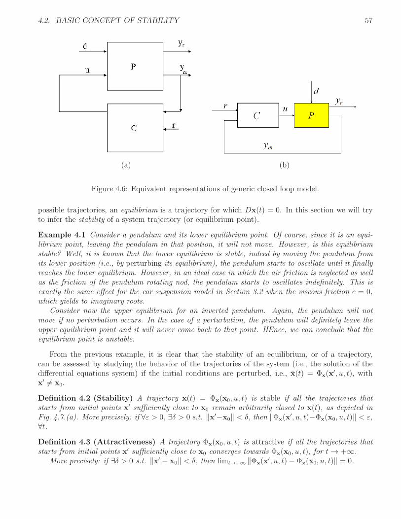
4.2. BASIC CONCEPT OF STABILITY 57
(a) (b)
Figure 4.6: Equivalent representations of generic closed loop model.
possible trajectories, an equilibrium is a trajectory for which Dx(t) = 0. In this section we will tryto infer the stability of a system trajectory (or equilibrium point).
Example 4.1 Consider a pendulum and its lower equilibrium point. Of course, since it is an equi-librium point, leaving the pendulum in that position, it will not move. However, is this equilibriumstable? Well, it is known that the lower equilibrium is stable, indeed by moving the pendulum fromits lower position (i.e., by perturbing its equilibrium), the pendulum starts to oscillate until it finallyreaches the lower equilibrium. However, in an ideal case in which the air friction is neglected as wellas the friction of the pendulum rotating nod, the pendulum starts to oscillates indefinitely. This isexactly the same effect for the car suspension model in Section 3.2 when the viscous friction c = 0,which yields to imaginary roots.
Consider now the upper equilibrium for an inverted pendulum. Again, the pendulum will notmove if no perturbation occurs. In the case of a perturbation, the pendulum will definitely leave theupper equilibrium point and it will never come back to that point. HEnce, we can conclude that theequilibrium point is unstable.
From the previous example, it is clear that the stability of an equilibrium, or of a trajectory,can be assessed by studying the behavior of the trajectories of the system (i.e., the solution of thedifferential equations system) if the initial conditions are perturbed, i.e., x(t) = Φx(x
′, u, t), withx′ 6= x0.
Definition 4.2 (Stability) A trajectory x(t) = Φx(x0, u, t) is stable if all the trajectories thatstarts from initial points x′ sufficiently close to x0 remain arbitrarily closed to x(t), as depicted inFig. 4.7.(a). More precisely: if ∀ε > 0, ∃δ > 0 s.t. ‖x′−x0‖ < δ, then ‖Φx(x
′, u, t)−Φx(x0, u, t)‖ < ε,∀t.
Definition 4.3 (Attractiveness) A trajectory Φx(x0, u, t) is attractive if all the trajectories thatstarts from initial points x′ sufficiently close to x0 converges towards Φx(x0, u, t), for t→ +∞.
More precisely: if ∃δ > 0 s.t. ‖x′ − x0‖ < δ, then limt→+∞ ‖Φx(x′, u, t)− Φx(x0, u, t)‖ = 0.
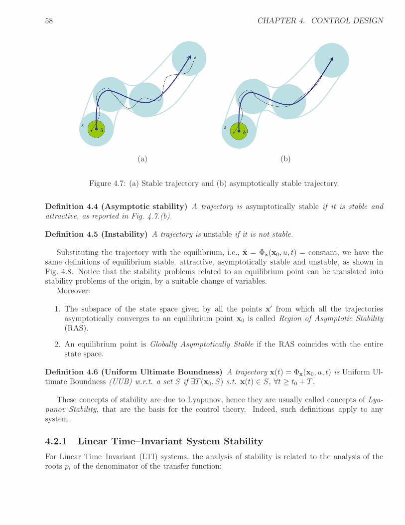
58 CHAPTER 4. CONTROL DESIGN
(a) (b)
Figure 4.7: (a) Stable trajectory and (b) asymptotically stable trajectory.
Definition 4.4 (Asymptotic stability) A trajectory is asymptotically stable if it is stable andattractive, as reported in Fig. 4.7.(b).
Definition 4.5 (Instability) A trajectory is unstable if it is not stable.
Substituting the trajectory with the equilibrium, i.e., x = Φx(x0, u, t) = constant, we have thesame definitions of equilibrium stable, attractive, asymptotically stable and unstable, as shown inFig. 4.8. Notice that the stability problems related to an equilibrium point can be translated intostability problems of the origin, by a suitable change of variables.
Moreover:
1. The subspace of the state space given by all the points x′ from which all the trajectoriesasymptotically converges to an equilibrium point x0 is called Region of Asymptotic Stability(RAS).
2. An equilibrium point is Globally Asymptotically Stable if the RAS coincides with the entirestate space.
Definition 4.6 (Uniform Ultimate Boundness) A trajectory x(t) = Φx(x0, u, t) is Uniform Ul-timate Boundness (UUB) w.r.t. a set S if ∃T (x0, S) s.t. x(t) ∈ S, ∀t ≥ t0 + T .
These concepts of stability are due to Lyapunov, hence they are usually called concepts of Lya-punov Stability, that are the basis for the control theory. Indeed, such definitions apply to anysystem.
4.2.1 Linear Time–Invariant System Stability
For Linear Time–Invariant (LTI) systems, the analysis of stability is related to the analysis of theroots pi of the denominator of the transfer function:
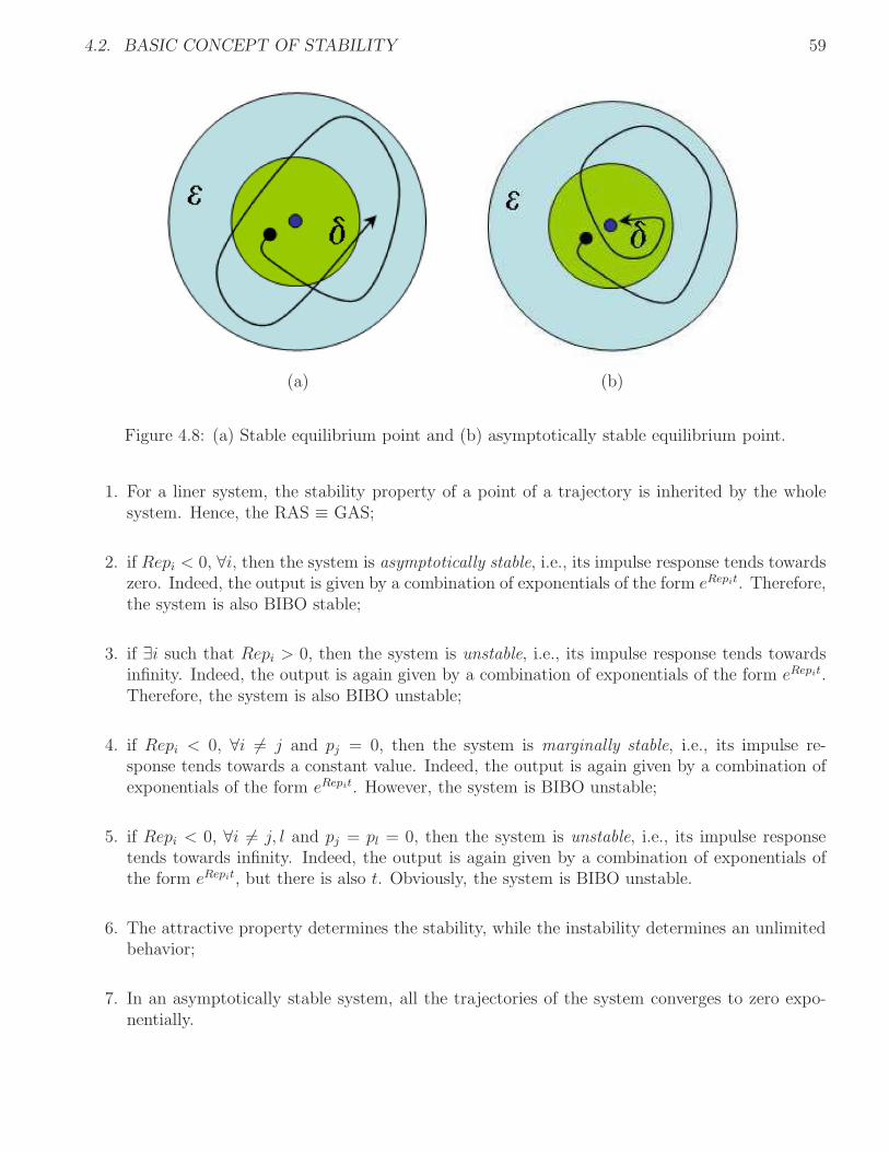
4.2. BASIC CONCEPT OF STABILITY 59
(a) (b)
Figure 4.8: (a) Stable equilibrium point and (b) asymptotically stable equilibrium point.
1. For a liner system, the stability property of a point of a trajectory is inherited by the wholesystem. Hence, the RAS ≡ GAS;
2. if Repi < 0, ∀i, then the system is asymptotically stable, i.e., its impulse response tends towardszero. Indeed, the output is given by a combination of exponentials of the form eRepit. Therefore,the system is also BIBO stable;
3. if ∃i such that Repi > 0, then the system is unstable, i.e., its impulse response tends towardsinfinity. Indeed, the output is again given by a combination of exponentials of the form eRepit.Therefore, the system is also BIBO unstable;
4. if Repi < 0, ∀i 6= j and pj = 0, then the system is marginally stable, i.e., its impulse re-sponse tends towards a constant value. Indeed, the output is again given by a combination ofexponentials of the form eRepit. However, the system is BIBO unstable;
5. if Repi < 0, ∀i 6= j, l and pj = pl = 0, then the system is unstable, i.e., its impulse responsetends towards infinity. Indeed, the output is again given by a combination of exponentials ofthe form eRepit, but there is also t. Obviously, the system is BIBO unstable.
6. The attractive property determines the stability, while the instability determines an unlimitedbehavior;
7. In an asymptotically stable system, all the trajectories of the system converges to zero expo-nentially.
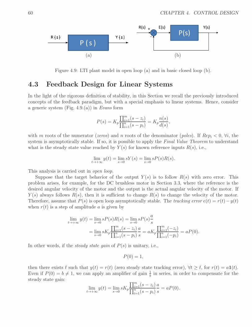
60 CHAPTER 4. CONTROL DESIGN
P ( s )
P(s)E(s) Y(s)R(s) +
-
(a) (b)
Figure 4.9: LTI plant model in open loop (a) and in basic closed loop (b).
4.3 Feedback Design for Linear Systems
In the light of the rigorous definition of stability, in this Section we recall the previously introducedconcepts of the feedback paradigm, but with a special emphasis to linear systems. Hence, considera generic system (Fig. 4.9.(a)) in Evans form
P (s) = Kp
∏m
i=1(s− zi)∏n
i=1(s− pi)= Kp
n(s)
d(s),
with m roots of the numerator (zeros) and n roots of the denominator (poles). If Repi < 0, ∀i, thesystem is asymptotically stable. If so, it is possible to apply the Final Value Theorem to understandwhat is the steady state value reached by Y (s) for known reference inputs R(s), i.e.,
limt→+∞
y(t) = lims→0
sY (s) = lims→0
sP (s)R(s).
This analysis is carried out in open loop.Suppose that the target behavior of the output Y (s) is to follow R(s) with zero error. This
problem arises, for example, for the DC brushless motor in Section 3.3, where the reference is thedesired angular velocity of the motor and the output is the actual angular velocity of the motor. IfY (s) always follows R(s), then it is sufficient to change R(s) to change the velocity of the motor.Therefore, assume that P (s) is open loop asymptotically stable. The tracking error e(t) = r(t)−y(t)when r(t) is a step of amplitude a is given by
limt→+∞
y(t) = lims→0
sP (s)R(s) = lims→0
sP (s)a
s
= lims→0
sKp
∏m
i=1(s− zi)∏n
i=1(s− pi)
a
s= aKp
∏m
i=1(−zi)∏n
i=1(−pi)= aP (0).
In other words, if the steady state gain of P (s) is unitary, i.e.,
P (0) = 1,
then there exists t such that y(t) = r(t) (zero steady state tracking error), ∀t ≥ t, for r(t) = a1(t).Even if P (0) = b 6= 1, we can apply an amplifier of gain 1
bin series, in order to compensate for the
steady state gain:
limt→+∞
y(t) = lims→0
sKp
∏m
i=1(s− zi)∏n
i=1(s− pi)
a
s= aP (0).
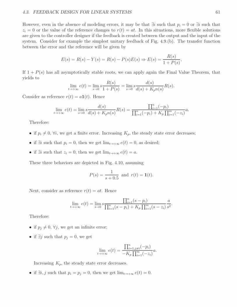
4.3. FEEDBACK DESIGN FOR LINEAR SYSTEMS 61
However, even in the absence of modeling errors, it may be that ∃i such that pi = 0 or ∃i such thatzi = 0 or the value of the reference changes to r(t) = at. In this situations, more flexible solutionsare given to the controller designer if the feedback is created between the output and the input of thesystem. Consider for example the simplest unitary feedback of Fig. 4.9.(b). The transfer functionbetween the error and the reference will be given by
E(s) = R(s)− Y (s) = R(s)− P (s)E(s)⇒ E(s) =R(s)
1 + P (s),
If 1 + P (s) has all asymptotically stable roots, we can apply again the Final Value Theorem, thatyields to
limt→+∞
e(t) = lims→0
sR(s)
1 + P (s)= lim
s→0s
d(s)
d(s) +Kpn(s)R(s).
Consider as reference r(t) = a1(t). Hence
limt→+∞
e(t) = lims→0
sd(s)
d(s) +Kpn(s)R(s) =
∏n
i=1(−pi)∏n
i=1(−pi) +Kp
∏m
i=1(−zi)a.
Therefore:
• if pi 6= 0, ∀i, we get a finite error. Increasing Kp, the steady state error decreases;
• if ∃i such that pi = 0, then we get limt→+∞ e(t) = 0, as desired;
• if ∃i such that zi = 0, then we get limt→+∞ e(t) = a.
These three behaviors are depicted in Fig. 4.10, assuming
P (s) =1
s+ 0.5and r(t) = 1(t).
Next, consider as reference r(t) = at. Hence
limt→+∞
e(t) = lims→0
s
∏n
i=1(s− pi)∏n
i=1(s− pi) +Kp
∏m
i=1(s− zi)
a
s2.
Therefore:
• if pj 6= 0, ∀j, we get an infinite error;
• if ∃j such that pj = 0, we get
limt→+∞
e(t) =
∏n
i=1,j 6=i(−pi)−Kp
∏m
i=1(−zi)a.
Increasing Kp, the steady state error decreases.
• if ∃i, j such that pi = pj = 0, then we get limt→+∞ e(t) = 0.
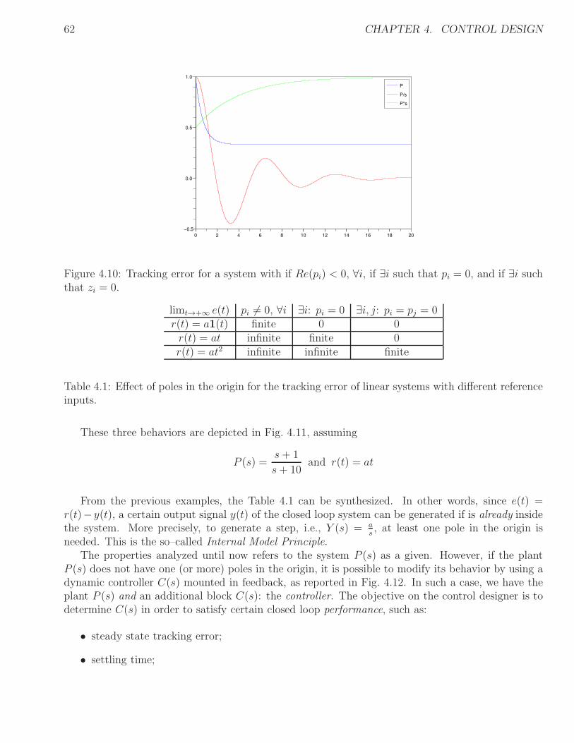
62 CHAPTER 4. CONTROL DESIGN
0 2 4 6 8 10 12 14 16 18 20
−0.5
0.0
0.5
1.0
P
P/s
P*s
Figure 4.10: Tracking error for a system with if Re(pi) < 0, ∀i, if ∃i such that pi = 0, and if ∃i suchthat zi = 0.
limt→+∞ e(t) pi 6= 0, ∀i ∃i: pi = 0 ∃i, j: pi = pj = 0r(t) = a1(t) finite 0 0r(t) = at infinite finite 0r(t) = at2 infinite infinite finite
Table 4.1: Effect of poles in the origin for the tracking error of linear systems with different referenceinputs.
These three behaviors are depicted in Fig. 4.11, assuming
P (s) =s+ 1
s+ 10and r(t) = at
From the previous examples, the Table 4.1 can be synthesized. In other words, since e(t) =r(t)− y(t), a certain output signal y(t) of the closed loop system can be generated if is already insidethe system. More precisely, to generate a step, i.e., Y (s) = a
s, at least one pole in the origin is
needed. This is the so–called Internal Model Principle.The properties analyzed until now refers to the system P (s) as a given. However, if the plant
P (s) does not have one (or more) poles in the origin, it is possible to modify its behavior by using adynamic controller C(s) mounted in feedback, as reported in Fig. 4.12. In such a case, we have theplant P (s) and an additional block C(s): the controller. The objective on the control designer is todetermine C(s) in order to satisfy certain closed loop performance, such as:
• steady state tracking error;
• settling time;
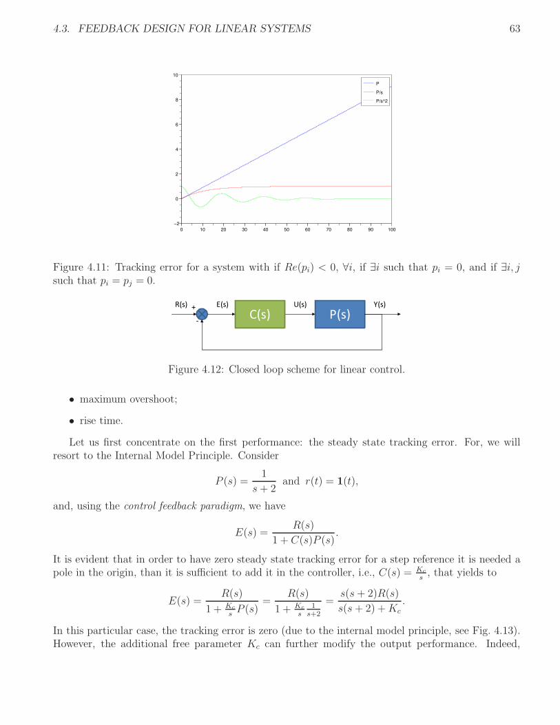
4.3. FEEDBACK DESIGN FOR LINEAR SYSTEMS 63
0 10 20 30 40 50 60 70 80 90 100
−2
0
2
4
6
8
10
P
P/s
P/s^2
Figure 4.11: Tracking error for a system with if Re(pi) < 0, ∀i, if ∃i such that pi = 0, and if ∃i, jsuch that pi = pj = 0.
P(s)U(s) Y(s)R(s) +
-C(s)
E(s)
Figure 4.12: Closed loop scheme for linear control.
• maximum overshoot;
• rise time.
Let us first concentrate on the first performance: the steady state tracking error. For, we willresort to the Internal Model Principle. Consider
P (s) =1
s+ 2and r(t) = 1(t),
and, using the control feedback paradigm, we have
E(s) =R(s)
1 + C(s)P (s).
It is evident that in order to have zero steady state tracking error for a step reference it is needed apole in the origin, than it is sufficient to add it in the controller, i.e., C(s) = Kc
s, that yields to
E(s) =R(s)
1 + Kc
sP (s)
=R(s)
1 + Kc
s1
s+2
=s(s+ 2)R(s)
s(s+ 2) +Kc
.
In this particular case, the tracking error is zero (due to the internal model principle, see Fig. 4.13).However, the additional free parameter Kc can further modify the output performance. Indeed,
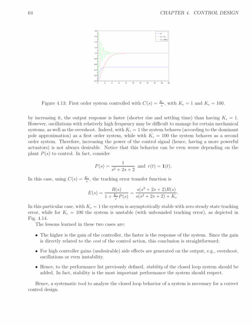
64 CHAPTER 4. CONTROL DESIGN
0 2 4 6 8 10 12 14 16 18 20
0.0
0.2
0.4
0.6
0.8
1.0
1.2
1.4
1.6
1.8
P
C = 1/s
C = 100/s
Figure 4.13: First order system controlled with C(s) = Kc
s, with Kc = 1 and Kc = 100.
by increasing it, the output response is faster (shorter rise and settling time) than having Kc = 1.However, oscillations with relatively high frequency may be difficult to manage for certain mechanicalsystems, as well as the overshoot. Indeed, withKc = 1 the system behaves (according to the dominantpole approximation) as a first order system, while with Kc = 100 the system behaves as a secondorder system. Therefore, increasing the power of the control signal (hence, having a more powerfulactuators) is not always desirable. Notice that this behavior can be even worse depending on theplant P (s) to control. In fact, consider
P (s) =1
s2 + 2s+ 2and r(t) = 1(t).
In this case, using C(s) = Kc
s, the tracking error transfer function is
E(s) =R(s)
1 + Kc
sP (s)
=s(s2 + 2s+ 2)R(s)
s(s2 + 2s+ 2) +Kc
.
In this particular case, withKc = 1 the system is asymptotically stable with zero steady state trackingerror, while for Kc = 100 the system is unstable (with unbounded tracking error), as depicted inFig. 4.14.
The lessons learned in these two cases are:
• The higher is the gain of the controller, the faster is the response of the system. Since the gainis directly related to the cost of the control action, this conclusion is straightforward;
• For high controller gains (undesirable) side effects are generated on the output, e.g., overshoot,oscillations or even instability.
• Hence, to the performance list previously defined, stability of the closed loop system should beadded. In fact, stability is the most important performance the system should respect.
Hence, a systematic tool to analyze the closed loop behavior of a system is necessary for a correctcontrol design.
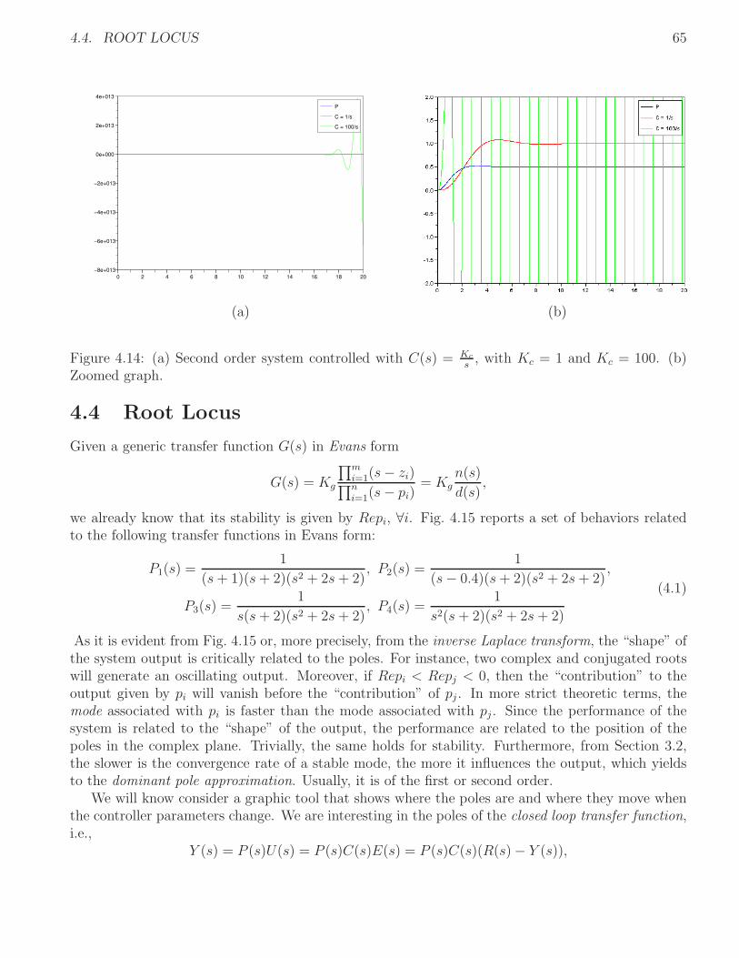
4.4. ROOT LOCUS 65
0 2 4 6 8 10 12 14 16 18 20
−8e+013
−6e+013
−4e+013
−2e+013
0e+000
2e+013
4e+013
P
C = 1/s
C = 100/s
(a) (b)
Figure 4.14: (a) Second order system controlled with C(s) = Kc
s, with Kc = 1 and Kc = 100. (b)
Zoomed graph.
4.4 Root Locus
Given a generic transfer function G(s) in Evans form
G(s) = Kg
∏m
i=1(s− zi)∏n
i=1(s− pi)= Kg
n(s)
d(s),
we already know that its stability is given by Repi, ∀i. Fig. 4.15 reports a set of behaviors relatedto the following transfer functions in Evans form:
P1(s) =1
(s+ 1)(s+ 2)(s2 + 2s+ 2), P2(s) =
1
(s− 0.4)(s+ 2)(s2 + 2s+ 2),
P3(s) =1
s(s+ 2)(s2 + 2s+ 2), P4(s) =
1
s2(s+ 2)(s2 + 2s+ 2)
(4.1)
As it is evident from Fig. 4.15 or, more precisely, from the inverse Laplace transform, the “shape” ofthe system output is critically related to the poles. For instance, two complex and conjugated rootswill generate an oscillating output. Moreover, if Repi < Repj < 0, then the “contribution” to theoutput given by pi will vanish before the “contribution” of pj . In more strict theoretic terms, themode associated with pi is faster than the mode associated with pj . Since the performance of thesystem is related to the “shape” of the output, the performance are related to the position of thepoles in the complex plane. Trivially, the same holds for stability. Furthermore, from Section 3.2,the slower is the convergence rate of a stable mode, the more it influences the output, which yieldsto the dominant pole approximation. Usually, it is of the first or second order.
We will know consider a graphic tool that shows where the poles are and where they move whenthe controller parameters change. We are interesting in the poles of the closed loop transfer function,i.e.,
Y (s) = P (s)U(s) = P (s)C(s)E(s) = P (s)C(s)(R(s)− Y (s)),
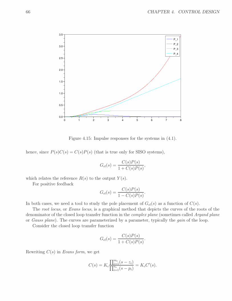
66 CHAPTER 4. CONTROL DESIGN
0 1 2 3 4 5 6 7 8
0.0
0.5
1.0
1.5
2.0
2.5
3.0
3.5
P_1
P_2
P_3
P_4
Figure 4.15: Impulse responses for the systems in (4.1).
hence, since P (s)C(s) = C(s)P (s) (that is true only for SISO systems),
Gcl(s) =C(s)P (s)
1 + C(s)P (s),
which relates the reference R(s) to the output Y (s).
For positive feedback
Gcl(s) =C(s)P (s)
1− C(s)P (s).
In both cases, we need a tool to study the pole placement of Gcl(s) as a function of C(s).
The root locus, or Evans locus, is a graphical method that depicts the curves of the roots of thedenominator of the closed loop transfer function in the complex plane (sometimes called Argand planeor Gauss plane). The curves are parameterized by a parameter, typically the gain of the loop.
Consider the closed loop transfer function
Gcl(s) =C(s)P (s)
1 + C(s)P (s).
Rewriting C(s) in Evans form, we get
C(s) = Kc
∏mc
i=1(s− zi)∏nc
i=1(s− pi)= KcC
′(s).

4.4. ROOT LOCUS 67
Similarly, for P (s)
P (s) = Kp
∏mp
i=1(s− zi)∏np
i=1(s− pi)= KpP
′(s).
The closed loop poles will be given by the solution of
1 + C(s)P (s) = 1 +KcC′(s)KpP
′(s) = 1 +KcKpG(s) = 0, (4.2)
where Kp is given by the plant model, Kc is the gain parameter of the controller and
G(s) = C ′(s)P ′(s) =n(s)
d(s). (4.3)
Since G(s) is a complex function, the equation (4.2) is satisfied for any value of 0 ≤ Kc ≤ +∞ if:
• Modulus constraint:∣
∣
∣
∣
Kp
n(s)
d(s)
∣
∣
∣
∣
=1
Kc
,
which yields to∣
∣
∣
∣
KcKp
n(s)
d(s)
∣
∣
∣
∣
= 1.
• Phase constraint:
∠n(s)
d(s)= ∠
1
−Kp
or, equivalently
m∑
i=1
∠(s− zi)−n
∑
i=1
∠(s− pi) =
π mod 2π, if Kp > 0
0 mod 2π, if Kp < 0,
where m = mc +mp and n = nc + np. This way, the sign of KcKpG(s) is negative.
Strictly speaking, a point s in the Gauss plane belongs to the root locus if the sum of thephases of the vectors starting from the singularities (poles or zeros) and ending on the point sis equal to π (or 0 if Kp < 0), as depicted in Fig. 4.16.
Remark 4.7 The constraint on the phase is sufficient to draw the entire locus. The correspondencebetween the position of the roots and the value of Kc is determined by the constraint on the modulus.
4.4.1 Root locus construction
Consider the subsequent equationd(s) +KcKpn(s) = 0,
that has the same roots of the previous equation. Hence:
• for Kc = 0, the roots are given by the n roots of d(s);
• for Kc → +∞, the roots are given by the m roots of n(s).
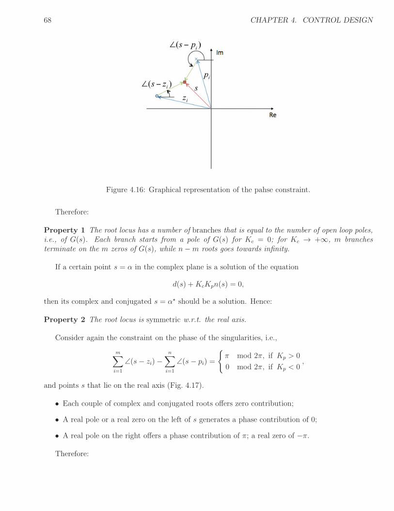
68 CHAPTER 4. CONTROL DESIGN
Figure 4.16: Graphical representation of the pahse constraint.
Therefore:
Property 1 The root locus has a number of branches that is equal to the number of open loop poles,i.e., of G(s). Each branch starts from a pole of G(s) for Kc = 0; for Kc → +∞, m branchesterminate on the m zeros of G(s), while n−m roots goes towards infinity.
If a certain point s = α in the complex plane is a solution of the equation
d(s) +KcKpn(s) = 0,
then its complex and conjugated s = α⋆ should be a solution. Hence:
Property 2 The root locus is symmetric w.r.t. the real axis.
Consider again the constraint on the phase of the singularities, i.e.,
m∑
i=1
∠(s− zi)−n
∑
i=1
∠(s− pi) =
π mod 2π, if Kp > 0
0 mod 2π, if Kp < 0,
and points s that lie on the real axis (Fig. 4.17).
• Each couple of complex and conjugated roots offers zero contribution;
• A real pole or a real zero on the left of s generates a phase contribution of 0;
• A real pole on the right offers a phase contribution of π; a real zero of −π.
Therefore:
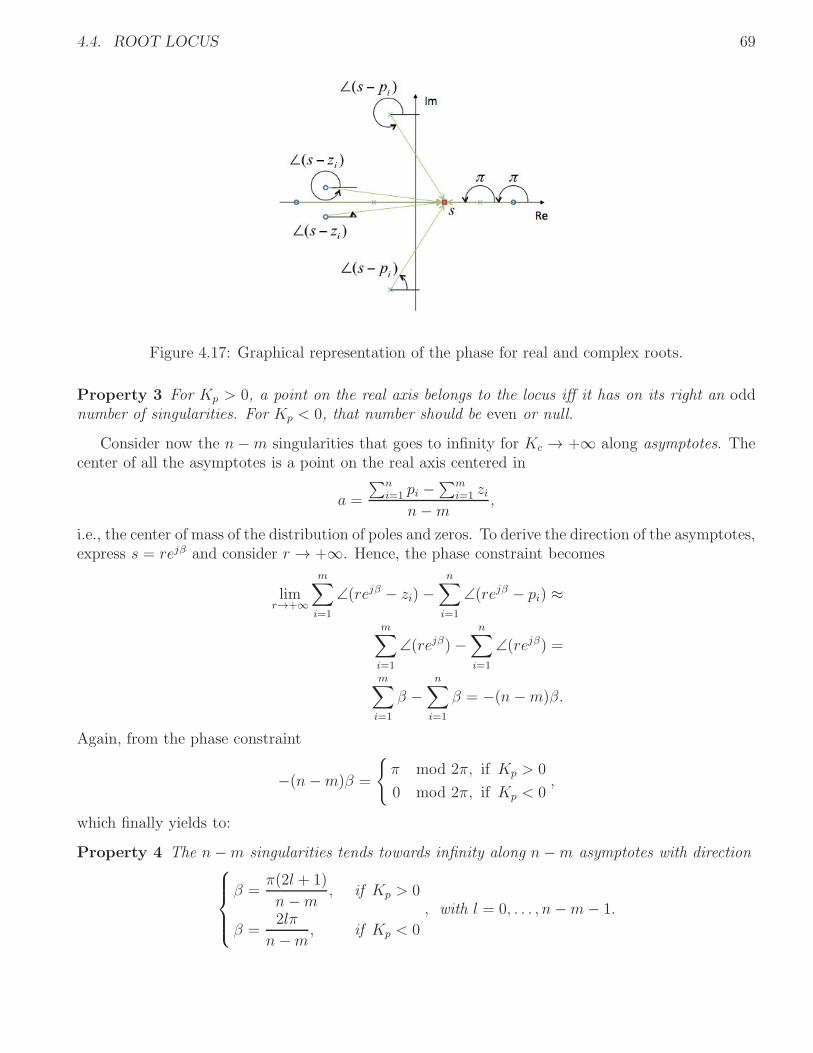
4.4. ROOT LOCUS 69
Figure 4.17: Graphical representation of the phase for real and complex roots.
Property 3 For Kp > 0, a point on the real axis belongs to the locus iff it has on its right an oddnumber of singularities. For Kp < 0, that number should be even or null.
Consider now the n−m singularities that goes to infinity for Kc → +∞ along asymptotes. Thecenter of all the asymptotes is a point on the real axis centered in
a =
∑n
i=1 pi −∑m
i=1 zin−m
,
i.e., the center of mass of the distribution of poles and zeros. To derive the direction of the asymptotes,express s = rejβ and consider r → +∞. Hence, the phase constraint becomes
limr→+∞
m∑
i=1
∠(rejβ − zi)−n
∑
i=1
∠(rejβ − pi) ≈
m∑
i=1
∠(rejβ)−n
∑
i=1
∠(rejβ) =
m∑
i=1
β −n
∑
i=1
β = −(n−m)β.
Again, from the phase constraint
−(n−m)β =
π mod 2π, if Kp > 0
0 mod 2π, if Kp < 0,
which finally yields to:
Property 4 The n−m singularities tends towards infinity along n−m asymptotes with direction
β =π(2l + 1)
n−m, if Kp > 0
β =2lπ
n−m, if Kp < 0
, with l = 0, . . . , n−m− 1.
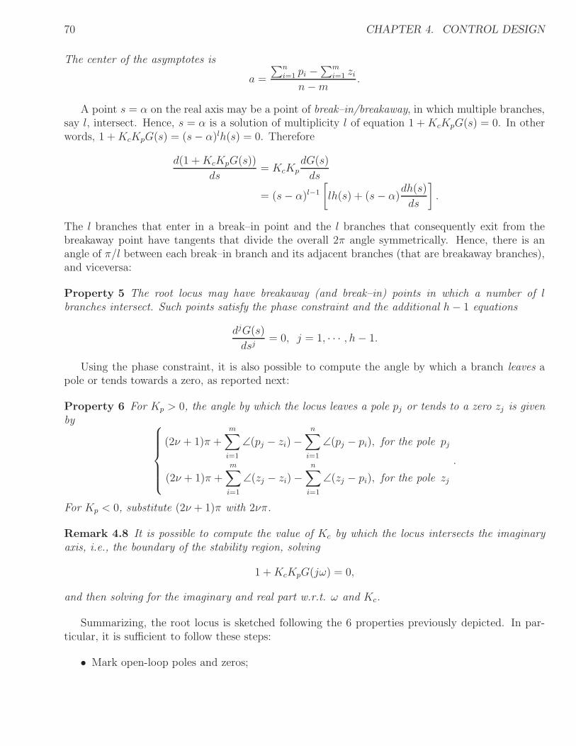
70 CHAPTER 4. CONTROL DESIGN
The center of the asymptotes is
a =
∑n
i=1 pi −∑m
i=1 zin−m
.
A point s = α on the real axis may be a point of break–in/breakaway, in which multiple branches,say l, intersect. Hence, s = α is a solution of multiplicity l of equation 1 +KcKpG(s) = 0. In otherwords, 1 +KcKpG(s) = (s− α)lh(s) = 0. Therefore
d(1 +KcKpG(s))
ds= KcKp
dG(s)
ds
= (s− α)l−1
[
lh(s) + (s− α)dh(s)
ds
]
.
The l branches that enter in a break–in point and the l branches that consequently exit from thebreakaway point have tangents that divide the overall 2π angle symmetrically. Hence, there is anangle of π/l between each break–in branch and its adjacent branches (that are breakaway branches),and viceversa:
Property 5 The root locus may have breakaway (and break–in) points in which a number of lbranches intersect. Such points satisfy the phase constraint and the additional h− 1 equations
djG(s)
dsj= 0, j = 1, · · · , h− 1.
Using the phase constraint, it is also possible to compute the angle by which a branch leaves apole or tends towards a zero, as reported next:
Property 6 For Kp > 0, the angle by which the locus leaves a pole pj or tends to a zero zj is givenby
(2ν + 1)π +
m∑
i=1
∠(pj − zi)−n
∑
i=1
∠(pj − pi), for the pole pj
(2ν + 1)π +m∑
i=1
∠(zj − zi)−n
∑
i=1
∠(zj − pi), for the pole zj
.
For Kp < 0, substitute (2ν + 1)π with 2νπ.
Remark 4.8 It is possible to compute the value of Kc by which the locus intersects the imaginaryaxis, i.e., the boundary of the stability region, solving
1 +KcKpG(jω) = 0,
and then solving for the imaginary and real part w.r.t. ω and Kc.
Summarizing, the root locus is sketched following the 6 properties previously depicted. In par-ticular, it is sufficient to follow these steps:
• Mark open-loop poles and zeros;
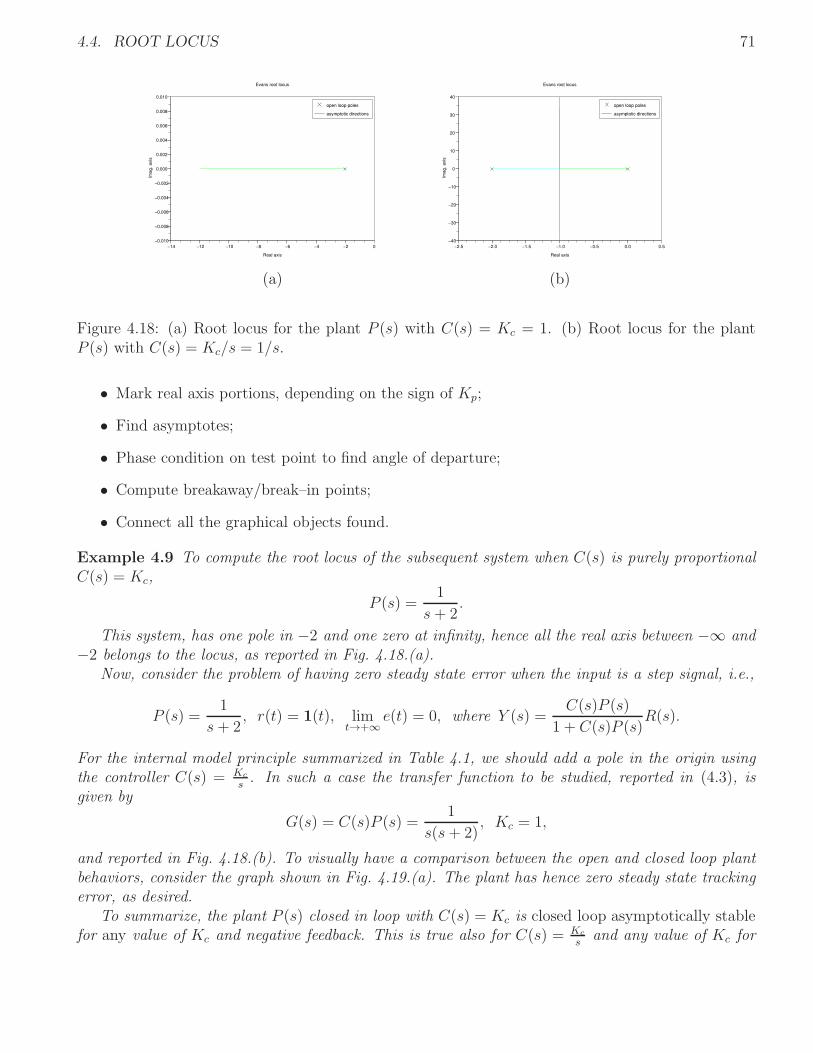
4.4. ROOT LOCUS 71
−14 −12 −10 −8 −6 −4 −2 0
−0.010
−0.008
−0.006
−0.004
−0.002
0.000
0.002
0.004
0.006
0.008
0.010
Evans root locus
Real axis
Ima
g.
axis
open loop poles
asymptotic directions
−2.5 −2.0 −1.5 −1.0 −0.5 0.0 0.5
−40
−30
−20
−10
0
10
20
30
40
Evans root locus
Real axis
Ima
g.
axis
open loop poles
asymptotic directions
(a) (b)
Figure 4.18: (a) Root locus for the plant P (s) with C(s) = Kc = 1. (b) Root locus for the plantP (s) with C(s) = Kc/s = 1/s.
• Mark real axis portions, depending on the sign of Kp;
• Find asymptotes;
• Phase condition on test point to find angle of departure;
• Compute breakaway/break–in points;
• Connect all the graphical objects found.
Example 4.9 To compute the root locus of the subsequent system when C(s) is purely proportionalC(s) = Kc,
P (s) =1
s+ 2.
This system, has one pole in −2 and one zero at infinity, hence all the real axis between −∞ and−2 belongs to the locus, as reported in Fig. 4.18.(a).
Now, consider the problem of having zero steady state error when the input is a step signal, i.e.,
P (s) =1
s+ 2, r(t) = 1(t), lim
t→+∞e(t) = 0, where Y (s) =
C(s)P (s)
1 + C(s)P (s)R(s).
For the internal model principle summarized in Table 4.1, we should add a pole in the origin usingthe controller C(s) = Kc
s. In such a case the transfer function to be studied, reported in (4.3), is
given by
G(s) = C(s)P (s) =1
s(s+ 2), Kc = 1,
and reported in Fig. 4.18.(b). To visually have a comparison between the open and closed loop plantbehaviors, consider the graph shown in Fig. 4.19.(a). The plant has hence zero steady state trackingerror, as desired.
To summarize, the plant P (s) closed in loop with C(s) = Kc is closed loop asymptotically stablefor any value of Kc and negative feedback. This is true also for C(s) = Kc
sand any value of Kc for
72 CHAPTER 4. CONTROL DESIGN
0 2 4 6 8 10 12 14 16 18 20
0.0
0.1
0.2
0.3
0.4
0.5
0.6
0.7
0.8
0.9
1.0
P
P_cl
−1 −0.8 −0.6 −0.4 −0.2 0 0.2 0.4 0.6 0.8 1−1
−0.8
−0.6
−0.4
−0.2
0
0.2
0.4
0.6
0.8
10.160.340.50.64
0.76
0.86
0.94
0.985
0.160.340.50.64
0.76
0.86
0.94
0.985
0.2
0.4
0.6
0.8
1
0.2
0.4
0.6
0.8
1
Root Locus
Real Axis
Imagin
ary
Axis
(a) (b)
Figure 4.19: (a) Open and closed loop responses to a unitary step reference. (b) Grid showing thedamping factor ξ and the natural frequency ωn on the root locus.
negative feedback. However, changing the value of the gain the overall output behavior changes. Asdepicted in Fig. 4.13, the output changes from a typical output of a first order to a second order one.This is due by the position of the closed loop poles, that univocally determine the response. Using theapproximation by the dominant pole, the closest to the imaginary axis is the slower pole, hence thedominant (since it has the smaller real part). Analytically, for Kc = 1 we have two coincident realroots in s1,2 = −1. For Kc = 100, we have two complex and conjugated roots in s1,2 = −1± 10j.
4.4.2 Analysis of a Second Order System in the Root Locus
The characteristic of a second order system are given by the values of the damping ξ factor and ofthe natural frequency ωn (see Section 3.2.3). Considering only two complex and conjugated roots,the closed loop plant can be described as
G(s) =1
s2
ω2n+ 2 ξ
ωns+ 1
.
For example, this is the case of Example 4.9, where forKc = 100 we have two complex and conjugatedroots in s1,2 = −1 ± 10j, with unitary steady state gain by the presence of a pole in the origin forthe controller C(s). Recalling Section 3.2.3, the roots of G(s) are of the form:
s1,2 = −ξωn ± ωn
√
1− ξ2,
therefore
ξ = cos(π − arctan 2(Im(s1), Re(s1)) and ωn = 1/|Re(s1)|.The values of ξ and ωn are depicted using a grid superimposed to the root locus in Fig. 4.19.(b).
To summarize, it is evident that we can model the performance of the system, i.e., rise time,settling time, overshoot, rather then simple stability, using the root locus and the first or secondorder dominant pole approximation.

4.5. BIBLIOGRAPHY 73
4.5 Bibliography
Chapter 5
Digital Control
The control law for the motor control synthesized using the root locus method is continuous time,i.e., it continuously measures the angular velocity of the motor and computes the control input.However, the control law should be implemented in a digital embedded platform. Therefore, thecontrol law has to be properly sampled in order to obtain a discrete time controller. This chapterpresents a methodology to discretize a continuous time system and then implement it on a digitalembedded platform. The references on this subject are [Oga95] and [AW96]. For the details aboutthe particular Operating System used on the Lego Mindstorm, the reader is referred to [Chi].
5.1 Discretization of Linear Continuous Time Controllers
Linear continuous time controllers need to be discretized in order to be implemented in a digital em-bedded system, i.e., to be implemented by an algorithm. Discretization is the process of transferringcontinuous models into discrete models. In the case of a dynamic system, the models are transferredfrom continuous time to discrete time, hence obtaining a discrete time controller. Therefore, thesystem is sampled using a well defined sampling time. In embedded-control systems, the samplingtime is usually lower bounded by feasibility reasons.
In practice, discretizing a continuous time system comprises the following steps:
• The plant measurements, e.g., the angular velocity of a motor shaft, are discretized using asampler, i.e., a A/D converter. The most common sampler is the zero–order hold, aka sample& hold.
• The sampled measurements are passed to the algorithm implementing the digital controller.
• The result of the computation is then given to a data reconstructor, i.e., a D/A converter,which reconstruct the continuous signal to be fed to the plant in a continuous piecewise signal.
There exist different solutions to discretize a system. A trivial solution may be to use a samplingtime that is the smaller possible, while keeping the controller continuous and using numeric toolsfor differential equations. Alternatively, there are different solutions that tries to minimize the dis-cretization approximations, which can be applied to transfer functions G(s) or to state space models.In this case, the approximation introduced are strictly related to the discrete time approximation ofthe integral of a continuous function.
74
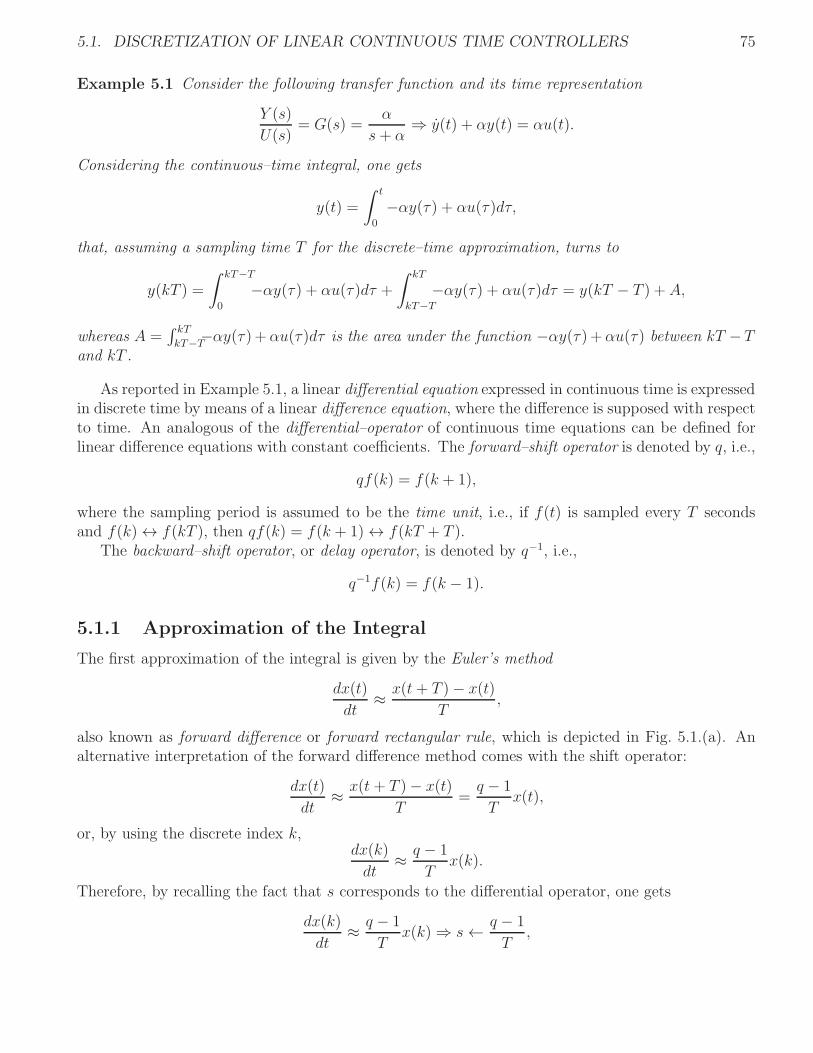
5.1. DISCRETIZATION OF LINEAR CONTINUOUS TIME CONTROLLERS 75
Example 5.1 Consider the following transfer function and its time representation
Y (s)
U(s)= G(s) =
α
s+ α⇒ y(t) + αy(t) = αu(t).
Considering the continuous–time integral, one gets
y(t) =
∫ t
0
−αy(τ) + αu(τ)dτ,
that, assuming a sampling time T for the discrete–time approximation, turns to
y(kT ) =
∫ kT−T
0
−αy(τ) + αu(τ)dτ +
∫ kT
kT−T
−αy(τ) + αu(τ)dτ = y(kT − T ) + A,
whereas A =∫ kT
kT−T−αy(τ) +αu(τ)dτ is the area under the function −αy(τ) +αu(τ) between kT − T
and kT .
As reported in Example 5.1, a linear differential equation expressed in continuous time is expressedin discrete time by means of a linear difference equation, where the difference is supposed with respectto time. An analogous of the differential–operator of continuous time equations can be defined forlinear difference equations with constant coefficients. The forward–shift operator is denoted by q, i.e.,
qf(k) = f(k + 1),
where the sampling period is assumed to be the time unit, i.e., if f(t) is sampled every T secondsand f(k)↔ f(kT ), then qf(k) = f(k + 1)↔ f(kT + T ).
The backward–shift operator, or delay operator, is denoted by q−1, i.e.,
q−1f(k) = f(k − 1).
5.1.1 Approximation of the Integral
The first approximation of the integral is given by the Euler’s method
dx(t)
dt≈ x(t + T )− x(t)
T,
also known as forward difference or forward rectangular rule, which is depicted in Fig. 5.1.(a). Analternative interpretation of the forward difference method comes with the shift operator:
dx(t)
dt≈ x(t + T )− x(t)
T=
q − 1
Tx(t),
or, by using the discrete index k,dx(k)
dt≈ q − 1
Tx(k).
Therefore, by recalling the fact that s corresponds to the differential operator, one gets
dx(k)
dt≈ q − 1
Tx(k)⇒ s← q − 1
T,
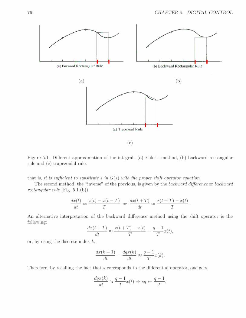
76 CHAPTER 5. DIGITAL CONTROL
(a) (b)
(c)
Figure 5.1: Different approximation of the integral: (a) Euler’s method, (b) backward rectangularrule and (c) trapezoidal rule.
that is, it is sufficient to substitute s in G(s) with the proper shift operator equation.
The second method, the “inverse” of the previous, is given by the backward difference or backwardrectangular rule (Fig. 5.1.(b))
dx(t)
dt≈ x(t)− x(t− T )
Tor
dx(t+ T )
dt≈ x(t+ T )− x(t)
T.
An alternative interpretation of the backward difference method using the shift operator is thefollowing:
dx(t+ T )
dt≈ x(t + T )− x(t)
T=
q − 1
Tx(t),
or, by using the discrete index k,
dx(k + 1)
dt=
dqx(k)
dt≈ q − 1
Tx(k).
Therefore, by recalling the fact that s corresponds to the differential operator, one gets
dqx(k)
dt≈ q − 1
Tx(t)⇒ sq ← q − 1
T,

5.1. DISCRETIZATION OF LINEAR CONTINUOUS TIME CONTROLLERS 77
and, more easily,
s← q − 1
qT,
that is again sufficient to substitute s in G(s) with the proper shift operator equation.Finally, the third and more accurate approximation of the integral is represented in Fig. 5.1.(c),
which is the trapezoidal rule, i.e.,∫ t2
t1
x(t)dt = (t2 − t1)x(t2)− x(t1)
2.
The trapezoidal rule can be interpreted as the integral of the time derivatives
1
2
(
dx(t+ T )
dt+
dx(t)
dt
)
≈ q − 1
Tx(t),
or, using the discrete index k,
1
2
(
dqx(k)
dt+
dx(k)
dt
)
≈ q − 1
Tx(k).
Therefore, by recalling the fact that s corresponds to the differential operator, one gets
1
2
(
dqx(k)
dt+
dx(k)
dt
)
≈ q − 1
Tx(k)⇒ qs+ s
2← q − 1
T
and, more easily,
s← 2
T
q − 1
q + 1.
Example 5.2 Consider the same system of Example 5.1. Using the forward rectangular rule, onegets
q − 1
Ty(k) + αy(k) = αu(k)⇒ y(k + 1) = (1− αT ) y(k) + αTu(k),
that is the difference equation that expresses the discrete–time approximation of Y (s) = G(s)U(s).Notice that the initial condition for y(k) is needed. The same result can be obtained by simply writethe equation in s and than substituting Y (s) with y(k), U(s) with u(k) and s with q−1
T. This is very
useful as soon as the transfer function has terms of the type sn.Instead, using the backward rectangular rule, one gets
q − 1
qTy(k) + αy(k) = αu(k)⇒ y(k + 1) =
y(k)
1 + αT+
αTu(k + 1)
1 + αT.
Notice that this time both the initial conditions for y(k) and for u(k) are needed. As before, it ssufficient to write the equation in s and than substituting Y (s) with y(k), U(s) with u(k) and s withq−1qT
.Finally, using the trapezoidal rule, one gets
2
T
q − 1
q + 1y(k) + αy(k) = αu(k)⇒ y(k + 1) =
2− αT
2 + αTy(k) +
αT
2 + αTu(k) +
αT
2 + αTu(k + 1).
Again, the initial conditions for y(k) and for u(k) are needed. AS in the previous cases, the sameresult can be obtained by simply write the equation in s and than substituting Y (s) with y(k), U(s)with u(k) and s with 2
T
q−1q+1
.
78 CHAPTER 5. DIGITAL CONTROL
5.1.2 Hints
A quite simple way to automatically discretize the system is to:
1. Substitute to the variable s in G(s) the function of the variable q;
2. Simplify the expressions of the numerator and the denominator;
3. The denominator will be multiplied by y(k), the numerator by u(k);
4. The coefficients of the two polynomials in q are the coefficients of y(k), i.e., (anqn + an−1q
n−1 + · · ·+ a1qturns to any(k + n) + an−1y(k + n− 1) + · · ·+ a1y(k + 1) + a0y(k). The same for u(k).
The most accurate discretization algorithm among the previous is the one given by the trapezoidalrule. Indeed, it gives the best approximation of the integral operator. More precisely:
• The forward difference may generate an unstable discrete–time system starting from a stablecontinuous–time system;
• The backward difference may generate stable discrete–time systems starting from unstablecontinuous–time systems;
• The trapezoidal rule maps continuous–time stable systems into discrete–time stable systemsand unstable into unstable systems.
Remark 5.3 Usually, the shift operator is a convenient way to express the complex variable z, thevariable of the Z–transform, that is the discrete time counterpart of the Laplace transform. As longas the Z–transform is considered, the approximation of the trapezoidal rule is also called Tustin’sapproximation or bilinear transformation. The Tustin approximation is derived by the approximationof the continuous time delay of the sampling time T , i.e.,
z = esT ≈ 1 + sT/2
1− sT/2,
which is the Pade approximant of the first order.
5.2 Multitask Implementation
Osek [Chi] is an open standard for embedded system architectures. NXTOsek Comprises NXT devicedrivers, a kernel and an operating system. It provides C and C++ programming environment (withGCC tool chain) and API for NXT sensors, actuators and other devices.
To use efficiently the NXTOsek, the following components are needed:
• GNU ARM compiler;
• Updated NXT Firmware to John Hansen’s Enhanced NXT firmware;
• NXTOsek set up.

5.3. BIBLIOGRAPHY 79
Figure 5.2: OIL file for the Hello world example.
An NXTOsek program consists of two parts: an OIL (Osek Implementation Language) and aC/C++ source code. The OIL is basically a file describing the architectures of the scheduler, thetasks (e.g., priority, activation, autostart), etc.. Once the OIL and the C/C++ coded files arecompiled, an RXE file is generated, which has to be downloaded (via USB) on the Lego NXT brickusing the rxeflash.sh.
Fig. 5.2 reports an OIL file for the Hello world example, which is coded in Fig. 5.3.
Fig. 5.4 reports an example code for a program that reads the light sensor and displays it on theLego brick.
Finally, Fig. 5.5 shows the code for a periodic task.
5.3 Bibliography
[AW96] K.J. Astrom and B. Wittenmark, Computer Controlled Systems, Prentice Hall Inc., Novem-ber 1996.
[Chi] Takashi Chikamasa, http://lejos-osek.sourceforge.net/.
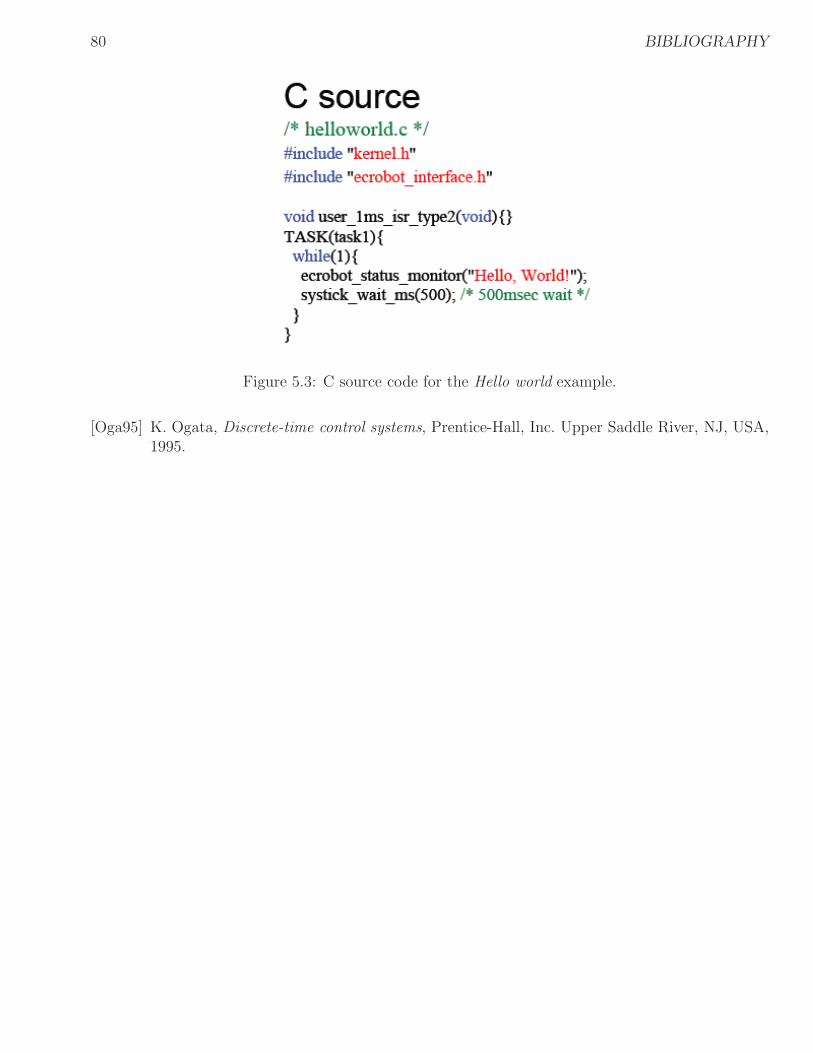
80 BIBLIOGRAPHY
Figure 5.3: C source code for the Hello world example.
[Oga95] K. Ogata, Discrete-time control systems, Prentice-Hall, Inc. Upper Saddle River, NJ, USA,1995.
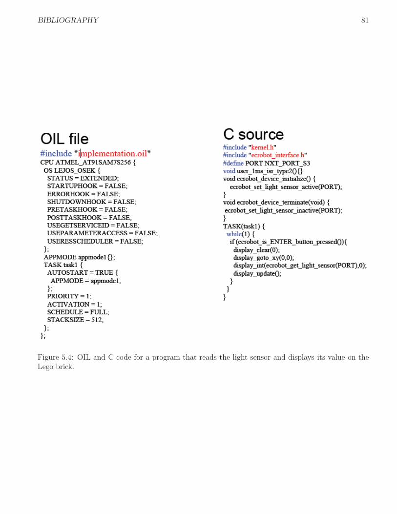
BIBLIOGRAPHY 81
Figure 5.4: OIL and C code for a program that reads the light sensor and displays its value on theLego brick.

82 BIBLIOGRAPHY
Figure 5.5: OIL and C code for a task with periodic activation.
Chapter 6
Simulation and Control of a WheeledRobot
The robotic system adopted for the project is a unicycle–like vehicle, which is a wheeled mobile robot(WMR) with differential drive [SSVO08]. First, a rigorous methodology to derive the kinematicmodel of a vehicle (and in particular of a unicycle) is presented. Since the model is non-linear, it willbe linearized using first order Taylor approximation. It is then possible to derive a controller for thelinearized system using the root locus.
6.1 Kinematic Model of the Robot
Consider a mechanical system whose configuration q ∈ Rn is described by a vector of generalized
coordinates, where the space of all possible robot configurations coincides with Rn. The motion of the
system, that is represented by the evolution of q over time, may be subject to constraints that canbe classified under various criteria. For example, they may be expressed as equalities or inequalities(respectively, bilateral or unilateral constraints). For simplicity’s sake, only bilateral constraints willbe considered in what follows.
Assume that a subset of coordinates qii, with i = 1, . . . , r ≤ n, is subjected to some bilateralconstraints. Such constraints can be related to positions q or velocity q. Constraints that are onlyfunction of the positions can be expressed as
h(q, t) = 0.
In this case, since the constraint depends explicitly from time, it is called rheonomic. In the subse-quent, only scleronomic constraints will be considered (time invariant), i.e.,
h(q) = 0,
where h(q) is a vector function with r entries, i.e., h(q) = [h1(q), . . . ,hr(q)]T , one for each constraint.
Such constraints, are called holonomic (or integrable). The effect of holonomic constraints is to reducethe space of accessible configurations to a subset of Rn with dimension R
n−r. A mechanical systemfor which all the constraints can be expressed in the form is called holonomic.
In the presence of holonomic constraints, the implicit function theorem, or Dini theorem, canbe used to express r generalized coordinates as a function of the remaining n− r, so as to actually
83
84 CHAPTER 6. SIMULATION AND CONTROL OF A WHEELED ROBOT
eliminate them from the formulation of the problem. However, due to singularities this proceduremay introduce, it is more convenient to replace the original generalized coordinates with a reducedset of n − r new coordinates that are directly defined on the accessible subspace. Noticing that,holonomic constraints are generally the result of mechanical interconnections between the variousbodies of the system, prismatic and revolute joints used in robot manipulators are a typical sourceof holonomic constraints, and joint variables are an example of reduced sets of coordinates.
Constraints that involve generalized coordinates and velocities
c(q,q) = 0,
where c(q,q) is a vector function with r entries, i.e., c(q,q) = [c1(q,q), . . . , cr(q,q)]T , are called
kinematic constraints. Such constrains limit the instantaneous admissible motion of the mechanicalsystem by reducing the set of generalized velocities that can be attained at each configuration. Kine-matic constraints are generally linear in the generalized velocities and hence they can be expressedas
ci(q)q = 0,
and, hence, can be expressed in a more compact Pfaffian form
A(q)q = 0.
ci(q)q, i = 1, . . . , r, are assumed to be smooth as well as linearly independent, i.e., A(q) is offull rank. Clearly, the kinematic constraints of the Pfaffian form can be obtained from direct timederivation of holonomic constraints, i.e.,
dhi(q)
dt=
∂hi(q)
∂qq = 0⇒ ∂hi(q)
∂q= ci(q).
It is trivial that for a holonomic mechanical system, r kinematic constraints correspond to r holonomicconstraints, obtained by integration of the kinematic constraints. Unfortunately, this is not alwaysthe case, since there may be kinematic constraints that are not integrable. In this case, the constraintis called nonholonomic and the system it belongs is called in its turn nonholonomic.
Beyond the mechanical aspects that may generate a holonomic system rather than a nonholonomicone, the main difference between such systems is related to their mobility. Indeed, consider anintegrable kinematic constraint ci(q)q = 0. Its integral can be written as hi(q) = hi(q0), where q0 isthe initial robot configuration. Hence, since we have imposed a constraint, the motion of the systemwill be constrained to a level surface of the scalar function hi(q), defined by hi(q0) and of dimensionn− 1.
For nonholonomic systems, instead, only the velocities are constrained on a subspace of dimensionn− 1 given by the kinematic constraint. Nevertheless, the fact that the constraint is non-integrablemeans that there is no loss of accessibility to Rn. In other words, while the number of DOFs decreasesto n− 1 due to the constraint, the number of generalized coordinates q cannot be reduced, not evenlocally. This important property is extended to any number of nonholonomic constraints r < n.
Summarizing, holonomic constraints limit the accessibility of the mechanical structure (e.g., thejoints of a manipulator) while nonholonomic constraints impose a limit in the velocity space butpreserve the accessibility of the mechanical structure. In other words, nonholonomy constrained thesystem velocities q. In the kinematic model of the constrained nonholonomic system, the feasible
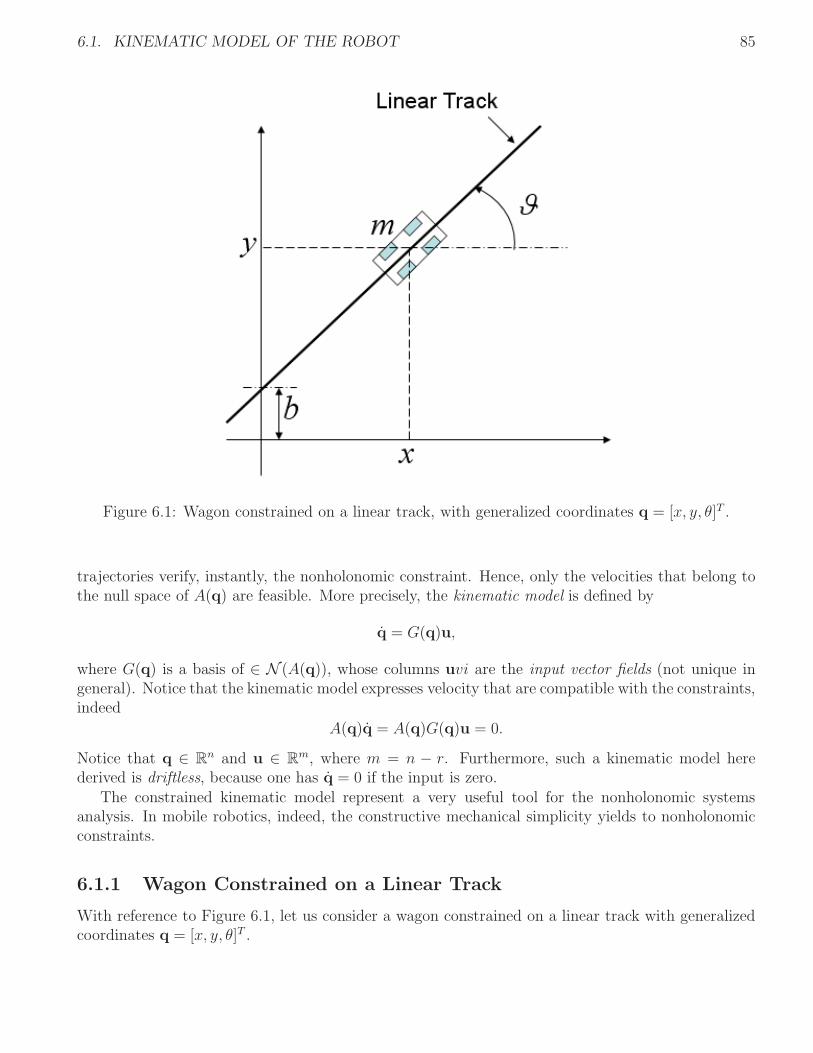
6.1. KINEMATIC MODEL OF THE ROBOT 85
Figure 6.1: Wagon constrained on a linear track, with generalized coordinates q = [x, y, θ]T .
trajectories verify, instantly, the nonholonomic constraint. Hence, only the velocities that belong tothe null space of A(q) are feasible. More precisely, the kinematic model is defined by
q = G(q)u,
where G(q) is a basis of ∈ N (A(q)), whose columns uvi are the input vector fields (not unique ingeneral). Notice that the kinematic model expresses velocity that are compatible with the constraints,indeed
A(q)q = A(q)G(q)u = 0.
Notice that q ∈ Rn and u ∈ R
m, where m = n − r. Furthermore, such a kinematic model herederived is driftless, because one has q = 0 if the input is zero.
The constrained kinematic model represent a very useful tool for the nonholonomic systemsanalysis. In mobile robotics, indeed, the constructive mechanical simplicity yields to nonholonomicconstraints.
6.1.1 Wagon Constrained on a Linear Track
With reference to Figure 6.1, let us consider a wagon constrained on a linear track with generalizedcoordinates q = [x, y, θ]T .
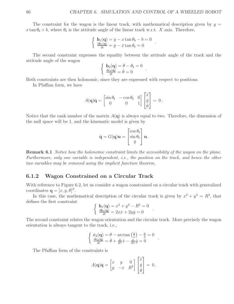
86 CHAPTER 6. SIMULATION AND CONTROL OF A WHEELED ROBOT
The constraint for the wagon is the linear track, with mathematical description given by y =x tan θb + b, where θb is the attitude angle of the linear track w.r.t. X axis. Therefore,
h1(q) = y − x tan θb − b = 0dh1(q)
dt= y − x tan θb = 0
.
The second constraint expresses the equality between the attitude angle of the track and theattitude angle of the wagon
h2(q) = θ − θb = 0dc2(q)
dt= θ = 0
.
Both constraints are then holonomic, since they are expressed with respect to positions.In Pfaffian form, we have
A(q)q =
[
sin θb − cos θb 00 0 1
]
xy
θ
= 0 .
Notice that the rank number of the matrix A(q) is always equal to two. Therefore, the dimension ofthe null space will be 1, and the kinematic model is given by
q = G(q)u =
cos θbsin θb0
u.
Remark 6.1 Notice how the holonomic constraint limits the accessibility of the wagon on the plane.Furthermore, only one variable is independent, i.e., the position on the track, and hence the othertwo variables may be removed using the implicit function theorem.
6.1.2 Wagon Constrained on a Circular Track
With reference to Figure 6.2, let us consider a wagon constrained on a circular track with generalizedcoordinates q = [x, y, θ]T .
In this case, the mathematical description of the circular track is given by x2 + y2 = R2, thatdefines the first constraint
h1(q) = x2 + y2 − R2 = 0dh1(q)
dt= 2xx+ 2yy = 0
.
The second constraint relates the wagon orientation and the circular track. More precisely the wagonorientation is always tangent to the track, i.e.,
c2(q) = θ − arctan(
y
x
)
− π2= 0
dc2(q)dt
= θ + y
R2 x− xR2 y = 0
.
The Pfaffian form of the constraints is
A(q)q =
[
x y 0y −x R2
]
xy
θ
= 0 .
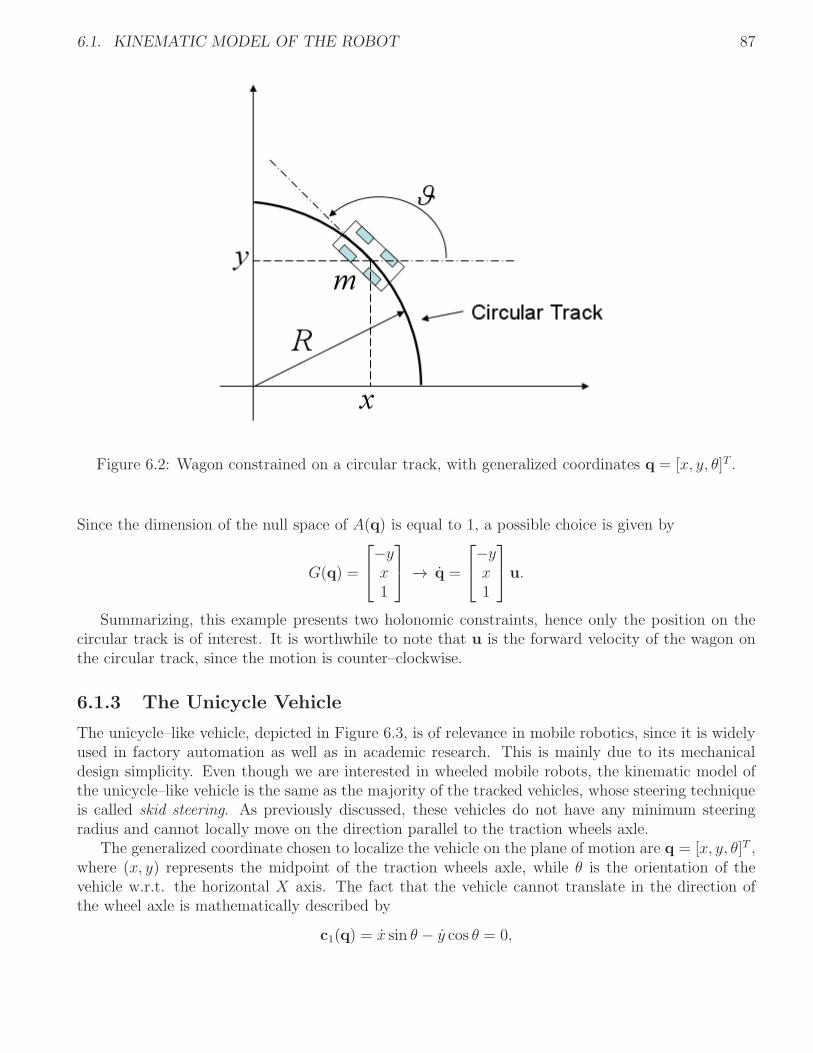
6.1. KINEMATIC MODEL OF THE ROBOT 87
Figure 6.2: Wagon constrained on a circular track, with generalized coordinates q = [x, y, θ]T .
Since the dimension of the null space of A(q) is equal to 1, a possible choice is given by
G(q) =
−yx1
→ q =
−yx1
u.
Summarizing, this example presents two holonomic constraints, hence only the position on thecircular track is of interest. It is worthwhile to note that u is the forward velocity of the wagon onthe circular track, since the motion is counter–clockwise.
6.1.3 The Unicycle Vehicle
The unicycle–like vehicle, depicted in Figure 6.3, is of relevance in mobile robotics, since it is widelyused in factory automation as well as in academic research. This is mainly due to its mechanicaldesign simplicity. Even though we are interested in wheeled mobile robots, the kinematic model ofthe unicycle–like vehicle is the same as the majority of the tracked vehicles, whose steering techniqueis called skid steering. As previously discussed, these vehicles do not have any minimum steeringradius and cannot locally move on the direction parallel to the traction wheels axle.
The generalized coordinate chosen to localize the vehicle on the plane of motion are q = [x, y, θ]T ,where (x, y) represents the midpoint of the traction wheels axle, while θ is the orientation of thevehicle w.r.t. the horizontal X axis. The fact that the vehicle cannot translate in the direction ofthe wheel axle is mathematically described by
c1(q) = x sin θ − y cos θ = 0,
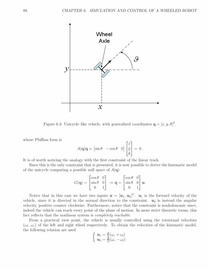
88 CHAPTER 6. SIMULATION AND CONTROL OF A WHEELED ROBOT
Figure 6.3: Unicycle–like vehicle, with generalized coordinates q = [x, y, θ]T .
whose Pfaffian form is
A(q)q =[
sin θ − cos θ 0]
xy
θ
= 0 .
It is of worth noticing the analogy with the first constraint of the linear track.Since this is the only constraint that is presented, it is now possible to derive the kinematic model
of the unicycle computing a possible null space of A(q)
G(q) =
cos θ 0sin θ 00 1
→ q =
cos θ 0sin θ 00 1
u.
Notice that in this case we have two inputs u = [u1, u2]T . u1 is the forward velocity of the
vehicle, since it is directed in the normal direction to the constraint. u2 is instead the angularvelocity, positive counter–clockwise. Furthermore, notice that the constraint is nonholonomic since,indeed the vehicle can reach every point of the plane of motion. In more strict theoretic terms, thisfact reflects that the nonlinear system is completely reachable.
From a practical view–point, the vehicle is usually controlled using the rotational velocities(ωl, ωr) of the left and right wheel respectively. To obtain the velocities of the kinematic model,the following relation are used
u1 =R2(ωr + ωl)
u2 =RD(ωr − ωl)
6.2. KINEMATIC LINEAR CONTROL 89
where R is the wheels radius and D is the length of the wheel axle.For space limitations, kinematic models of more complicated vehicles are not considered in these
notes (e.g., cooperative unicycles, bicycle, car–like). However, it is possible, using the presentedmathematic tools, to derive the kinematic model of any vehicle.
The dynamic models of the vehicles are not considered in these notes, since from a practicalviewpoint, most of the vehicles are controlled using the kinematic model. Indeed, it is possible todesign a low level controller that compensate for all the dynamic effects of the platform. This isexactly the linear controller implemented for the vehicle’s motors. In practice, the most popular andwidely used linear low level controller is the Proportional Integral Derivative (PID).
6.2 Kinematic Linear Control
In order to design a liner controller for the kinematic model of the unicycle, we need first to linearizeit using the Taylor approximation up to the first order. To this end, the equilibrium point aroundwhich the linearization operates is given by the problem at hand. Let us assume that the robot hasto be controlled around a desired path (path following problem, [SSVO08]), which is a straight line.Hence, assume that the straight line coincides with the X axis of the reference frame (this is notstrictly necessary, albeit this choice simplifies the equations). Furthermore, assume that the straightline is identified by a wall and that two sonars are used to measure the distance and the orientationof the vehicle from the wall. In such a situation, the kinematic model becomes:
qe =
xe
yeθe
=
cos θe 0sin θe 00 1
u,
where ye is the distance from the path and θe is the relative orientation between the robot andthe path. Since the path coincides with the X axis, the variable xe corresponds to the distancetravelled along the path, which cannot be measured by any available sensor (unless open loop deadreckoning is used, i.e., by integrating the value of the motor encoders, which generates a divergentestimate). Moreover, quantifying xe is not necessary if the target is to follow the path, indeed weare not interested in determine for “how long” the path is travelled along the X axis. Since xe doesnot influence the dynamic of the robot (which only depends on θe and u(t)), it can be neglected.Furthermore, we can assume that the forward velocity u1(t) is given and fixed to a constant u1(t) = v.With this choices, the nonlinear model turns to
qe =
[
yeθe
]
=
[
sin θev0
]
+
[
01
]
u2.
It is now possible to derive the linearized system using as linearization point the desired equilib-rium, i.e., qe = [0, 0]T and u2(t) = 0, which yields to the linear system
qe =
[
yeθe
]
=
[
θev0
]
+
[
01
]
u2.
The monolateral Laplace transform (assuming zero initial condition for both ye and θe) of thelinearized system yields to
[
sYe(s)sΘe(s)
]
=
[
Θe(s)v0
]
+
[
01
]
U2(s),
90 BIBLIOGRAPHY
that, solving the second equation for Θe(s) and then plugging it into the first equation give
Ye(s) =v
s2U2(s),
which is the transfer function of the problem. It is now possible to use the root locus approach inSection 4.4 to design a suitable controller satisfying the desired target performance and successivelydiscretize and implement it following the steps reported in Chapter 5 to finally have the robotfollowing the desired path.
6.2.1 Estimation Algorithms and Observers
In the design of the controller we have hypothesized that the output of the system ye(t) is availableby on-board sensors. However, this is not always possible. In the particular problem of measuringthe distance from a wall, for example, using the measurement coming from a single sonar on therobot is not sufficient. Indeed, the quantity ye(t) is the distance of the midpoint of the wheel axleto the wall, which is, by definition of distance, the line joining the midpoint of the wheel axle tothe wall and perpendicular to it. Therefore, to define this quantity it is necessary to determine theorientation of the vehicle with respect to the wall. The orientation can be derived by two measuresof the distance hence, either, using only one sonar in two successive positions or two sonars at thesame time.
The algorithm used to combine available sensorial data to infer the quantities of interest is calledan estimation algorithm, since every measure is affected by an error and, hence, only an estimate ofthe desired quantity can be reconstructed. In this class we can recognize image or signal processingalgorithms, digital filters, sensor fusion algorithms, etc.. It is important to note that each time thequantities of interest are the quantities that also define the dynamic of the system, e.g., ye and θe,then the estimator is called an observer. The observer is a dynamic system whose dynamic is givenby the model of the system to estimate. The interested reader can find a detailed description on thesubjet in [Kai80, AW96].
6.3 Bibliography
[AW96] K.J. Astrom and B. Wittenmark, Computer Controlled Systems, Prentice Hall Inc.,November 1996.
[Kai80] Thomas Kailath, Linear systems, vol. 1, Prentice-Hall Englewood Cliffs, NJ, 1980.
[SSVO08] B. Siciliano, L. Sciavicco, L. Villani, and G. Oriolo, Robotics: modelling, planning andcontrol, Springer Verlag, 2008.