Laboratory for Computational Proteomics

www.FenyoLab.org

E-mail: Info@FenyoLab.org

Facebook: NYUMC Computational Proteomics Laboratory

Twitter: @CompProteomics

computational proteomics

223

Chapter 14

Modeling Experimental Design for Proteomics

Jan Eriksson and David Fenyö

Abstract

The complexity of proteomes makes good experimental design essential for their successful investigation. Here, we describe how proteomics experiments can be modeled and how computer simulations of these models can be used to improve experimental designs.

Key words: Proteomics, Mass spectrometry, Experimental design, Simulations, Modeling

The proteomics researcher that aims at comprehensive proteome analysis using mass spectrometry (MS)-based methods will face experimental challenges. These challenges are due to the many different proteins encoded by a genome, the rich variation of protein posttranslational modifications, and the large concentra-tion differences between different proteins. The range of protein concentrations have been measured to be six orders of magni-tude in Saccharomyces cerevisiae (1) and estimated to be larger than ten orders of magnitude in body fluids (2). In contrast to these wide abundance ranges, the MS detection methods typi-cally employed in proteomics span only a few orders of magni-tude in range, hampering the identification and quantitation of low-abundance proteins. A good experimental design for pro-teomics should manage to keep the detection of low-abundance proteins and the cost for instrumentation and analysis at reason-able and desired levels.

Proteomics researchers have realized that the complexity and the range of protein abundance of a proteome make it necessary to apply various separation protocols prior to the MS-analysis.

1. Introduction

David Fenyö (ed.), Computational Biology, Methods in Molecular Biology, vol. 673,DOI 10.1007/978-1-60761-842-3_14, © Springer Science+Business Media, LLC 2010

224 Eriksson and Fenyö

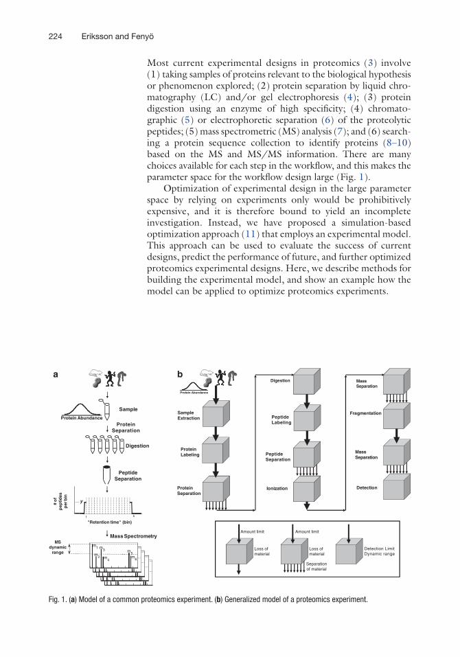
Most current experimental designs in proteomics (3) involve (1) taking samples of proteins relevant to the biological hypothesis or phenomenon explored; (2) protein separation by liquid chro-matography (LC) and/or gel electrophoresis (4); (3) protein digestion using an enzyme of high specificity; (4) chromato-graphic (5) or electrophoretic separation (6) of the proteolytic peptides; (5) mass spectrometric (MS) analysis (7); and (6) search-ing a protein sequence collection to identify proteins (8–10) based on the MS and MS/MS information. There are many choices available for each step in the workflow, and this makes the parameter space for the workflow design large (Fig. 1).

Optimization of experimental design in the large parameter space by relying on experiments only would be prohibitively expensive, and it is therefore bound to yield an incomplete investigation. Instead, we have proposed a simulation-based optimization approach (11) that employs an experimental model. This approach can be used to evaluate the success of current designs, predict the performance of future, and further optimized proteomics experimental designs. Here, we describe methods for building the experimental model, and show an example how the model can be applied to optimize proteomics experiments.

ProteinSeparation

PeptideSeparation

"Retention time" (bin)

y

1 k

# o

fp

eptid

esp

er b

in

Mass SpectrometryMS

dynamicrange

10

m1

m2

m3

m4

m5m6

Protein Abundance

Digestion

a

Sample

MassSeparation

Detection

MassSeparation

PeptideSeparation

PeptideLabeling

ProteinSeparation

Digestion

ProteinLabeling

SampleExtraction

Ionization

Fragmentation

Protein Abundance

Detection LimitDynamic range

Amount limit

Loss ofmaterial

Amount limit

Loss ofmaterial

Separationof material

b

Fig. 1. (a) Model of a common proteomics experiment. (b) Generalized model of a proteomics experiment.

225Modeling Experimental Design for Proteomics

Any computer simulation (see Note 1) needs input of reasonable assumptions about the model parameters in order to generate meaningful predictions about the experimental reality. The best overall strategy to improve experimental design is to use simula-tions together with good background information about the experimental components. In a general model of proteomics experiments there are many parameters (Fig. 1b), and many of these can be very difficult to determine (see Note 2), but often a simple model is sufficient to find the bottle-necks in the experi-mental design. The benefit of simulations is that once there is meaningful information available about parts of a system, this information can be employed in many different combinations in the computer to generate predictions much more rapidly than by experimental investigation. The simulations can also be used to determine which parameters are important to determine experi-mentally. Therefore, the proteomics researcher that would like to investigate and improve an experimental design should perform some model experiments or by other means determine the impor-tant model parameters. Pertinent information about all the parts that are important for the experimental design should be derived. The task can be viewed as containing three parts: (1) the protein sample, (2) the peptide sample, and (3) the mass spectrometry.

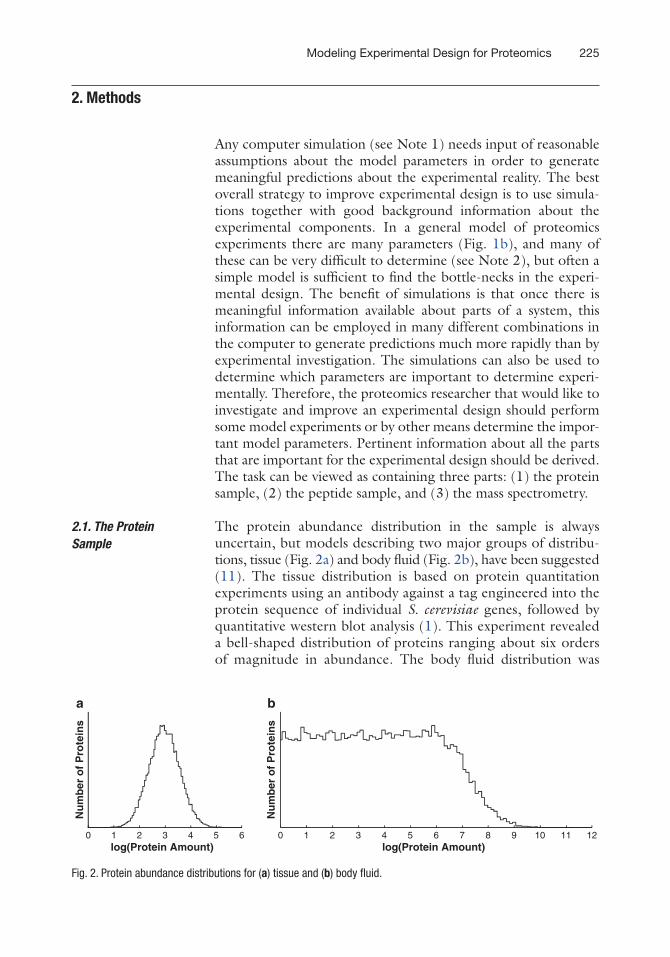
The protein abundance distribution in the sample is always uncertain, but models describing two major groups of distribu-tions, tissue (Fig. 2a) and body fluid (Fig. 2b), have been suggested (11). The tissue distribution is based on protein quantitation experiments using an antibody against a tag engineered into the protein sequence of individual S. cerevisiae genes, followed by quantitative western blot analysis (1). This experiment revealed a bell-shaped distribution of proteins ranging about six orders of magnitude in abundance. The body fluid distribution was

2. Methods

2.1. The Protein Sample

Nu

mb

er o

f P

rote

ins

log(Protein Amount)0 1 2 3 4 5 6 0 1 2 3 4 5 6 7 8 9 10 11 12

Nu

mb

er o

f P

rote

ins

log(Protein Amount)

a b

Fig. 2. Protein abundance distributions for (a) tissue and (b) body fluid.

226 Eriksson and Fenyö

assumed to cover a larger range of protein abundances (2), and to be bell-shaped at high abundances, and flat at low abundances. The flat shape at low abundances was chosen because many dif-ferent tissues in the body contribute proteins at a low level to the body fluid proteome. These distributions need to be calibrated based on the specific details of the experiment modeled. For example, these models do not take into account modified pro-teins. A scaling toward lower abundances is needed if, e.g., phos-pho-proteins are to be detected.

The next steps in the workflow that need to be modeled are protein separation by electrophoresis or chromatography and the subsequent digestion of the proteins with endoproteases. The losses associated with these steps need to be estimated. Here we refer this mixture of proteolytic peptides originating from the digested pro-teins as the peptide sample.

Separation of peptides is typically done using a reverse phase chromatography (RPC) column. The loading capacity and the resolving power of the RPC column should be estimated and incorporated in the model. The elution time of peptides in RPC is dependent on their sequence and can be estimated (12). There are many possible sources of losses for peptides: they can stick to walls, not bind to the column, or bind too hard to the column so that they cannot be eluted. All these losses are sequence depen-dent and difficult to elucidate in detail, but they can be estimated from model experiments.

In model experiments, samples from peptide libraries can be employed to estimate the detection sensitivity and dynamic range of the mass spectrometer. Note that the dynamic range of the mass spectrometer is the ratio of concentrations for two different peptide species that can be detected simultaneously, and it is much narrower than the range of concentrations over which a single peptide species can be detected when there are no other peptides in the sample. The rate of acquisition of the mass spectrometer can be determined in various modes of operation. In experimental designs with the mass spectrometer coupled online with the RPC column, the limited rate of acquisition will cause losses of peptides that are potentially detect-able. Other sources of losses in the mass spectrometry step include low ionization and fragmentation efficiencies.

Using a simple model for a typical proteomics experiment, we investigated the effect of changing the dynamic range and detec-tion limit of the mass spectrometer on the success rate and the

2.2. The Peptide Sample

2.3. The Mass Spectrometry

3. Results

227Modeling Experimental Design for Proteomics

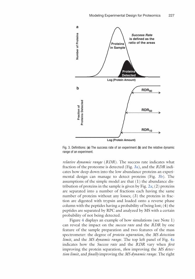
relative dynamic range (RDR). The success rate indicates what fraction of the proteome is detected (Fig. 3a), and the RDR indi-cates how deep down into the low abundance proteins an experi-mental design can manage to detect proteins (Fig. 3b). The assumptions of the simple model are that (1) the abundance dis-tribution of proteins in the sample is given by Fig. 2a; (2) proteins are separated into a number of fractions each having the same number of proteins without any losses; (3) the proteins in frac-tion are digested with trypsin and loaded onto a reverse phase column with the peptides having a probability of being lost; (4) the peptides are separated by RPC and analyzed by MS with a certain probability of not being detected.

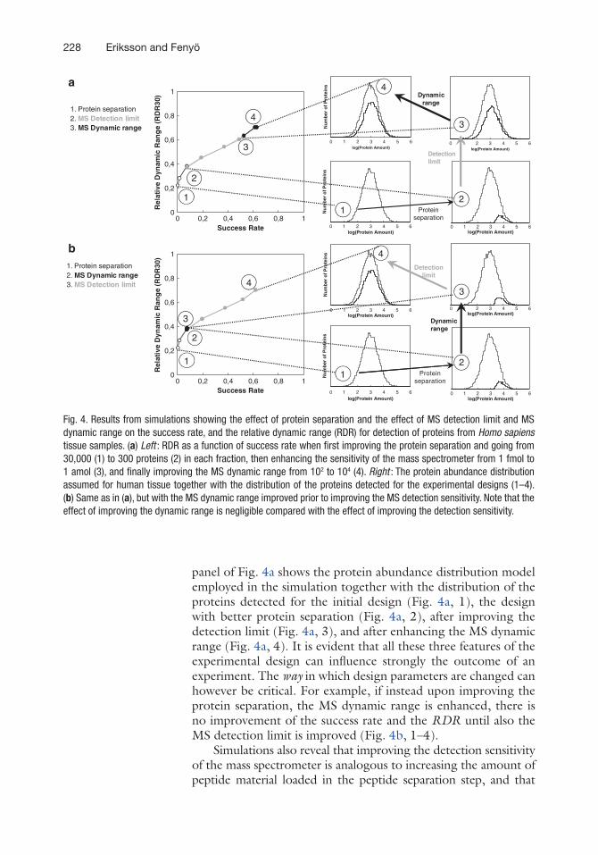
Figure 4 displays an example of how simulations (see Note 1) can reveal the impact on the success rate and the RDR by one feature of the sample preparation and two features of the mass spectrometer: the degree of protein separation, the MS detection limit, and the MS dynamic range. The top left panel of Fig. 4a indicates how the Success rate and the RDR vary when first improving the protein separation, then improving the MS detec-tion limit, and finally improving the MS dynamic range. The right

Nu

mb

er o

f P

rote

ins

ProteinsDetected

Success Rateis defined as theratio of the areasProteins

in Sample

Log (Protein Amount)

RDR90

RDR50

RDR10

Fra

ctio

n o

fP

rote

ins

Det

ecte

dLog (Protein Amount)

a

b

Fig. 3. Definitions: (a) The success rate of an experiment (b) and the relative dynamic range of an experiment.

228 Eriksson and Fenyö

panel of Fig. 4a shows the protein abundance distribution model employed in the simulation together with the distribution of the proteins detected for the initial design (Fig. 4a, 1), the design with better protein separation (Fig. 4a, 2), after improving the detection limit (Fig. 4a, 3), and after enhancing the MS dynamic range (Fig. 4a, 4). It is evident that all these three features of the experimental design can influence strongly the outcome of an experiment. The way in which design parameters are changed can however be critical. For example, if instead upon improving the protein separation, the MS dynamic range is enhanced, there is no improvement of the success rate and the RDR until also the MS detection limit is improved (Fig. 4b, 1–4).

Simulations also reveal that improving the detection sensitivity of the mass spectrometer is analogous to increasing the amount of peptide material loaded in the peptide separation step, and that

0

0,2

0,4

0,6

0,8

1

0 0,2 0,4 0,6 0,8 1Success Rate

Rel

ativ

e D

ynam

ic R

ang

e (R

DR

30)

0

0,2

0,4

0,6

0,8

1

0 0,2 0,4 0,6 0,8 1Success Rate

Rel

ativ

e D

ynam

ic R

ang

e (R

DR

30)

0 1 2 3 4 5 6log(Protein Amount)

Nu

mb

er o

f P

rote

ins

0 1 2 3 4 5 6log(Protein Amount)

Nu

mb

er o

f P

rote

ins

0 1 2 3 4 5 6log(Protein Amount)

0 1 2 3 4 5 6log(Protein Amount)

Nu

mb

er o

f P

rote

ins

0 1 2 3 4 5 6log(Protein Amount)

0 1 2 3 4 5 6log(Protein Amount)

0 1 2 3 4 5 6log(Protein Amount)

Nu

mb

er o

f P

rote

ins

0 1 2 3 4 5 6log(Protein Amount)

1. Protein separation2. MS Dynamic range3. MS Detection limit

1. Protein separation2. MS Detection limit3. MS Dynamic range

11

4

4

3

3

11

2

2

2

2

3

34

4

Proteinseparation

Detectionlimit

Dynamicrange

Proteinseparation

Dynamicrange

Detectionlimit

a

b

Fig. 4. Results from simulations showing the effect of protein separation and the effect of MS detection limit and MS dynamic range on the success rate, and the relative dynamic range (RDR) for detection of proteins from Homo sapiens tissue samples. (a) Left : RDR as a function of success rate when first improving the protein separation and going from 30,000 (1) to 300 proteins (2) in each fraction, then enhancing the sensitivity of the mass spectrometer from 1 fmol to 1 amol (3), and finally improving the MS dynamic range from 102 to 104 (4). Right : The protein abundance distribution assumed for human tissue together with the distribution of the proteins detected for the experimental designs (1–4). (b) Same as in (a), but with the MS dynamic range improved prior to improving the MS detection sensitivity. Note that the effect of improving the dynamic range is negligible compared with the effect of improving the detection sensitivity.

229Modeling Experimental Design for Proteomics

improving the MS dynamic range is analogous to enhancing the proteolytic peptide separation (11). The starting point in Fig. 4 assumes no protein separation, a load of 0.1 mg of peptides in the peptide separation step that separates the peptides into 100 frac-tions, and a mass spectrometer with a detection sensitivity of 1 fmol and a dynamic range of 100. This setup is not uncommon in pro-teomics, but is obviously the wrong choice for comprehensive anal-ysis. If comprehensive analysis is desired, Fig. 4 and results in ref. 11 show clearly that the practitioner should avoid the design (Fig. 4a, 1) and employ some protein separation and either load more material in the peptide separation step or choose a mass spec-trometer with better detection sensitivity prior to either improving separation of peptides or improving the MS dynamic range.

1. In the simulations, a mixture of human proteins is randomly selected. The estimated distribution of protein amounts in the sample (Fig. 2a) is used to assign an amount to each pro-tein in the mixture, and the protein mixture is digested. The resulting proteolytic peptides are randomly selected based on a precolumn survival probability. The surviving peptides are separated into fractions according to a separation model (12). The separated peptides are randomly selected based on a postcolumn survival probability. The surviving peptides are considered detected by MS if their amount is above the detec-tion limit and their peak intensity is within the dynamic range of the mass spectrometer. The entire process is repeated many times to obtain sufficient statistics.

2. A general model for a proteomics experiment has many parameters and it is often not feasible to determine many of them experimentally. An alternative to experimental determi-nation of model parameters is to investigate how sensitive the conclusions are to the model parameters. The experimental effort does not need to be focused on parameters that do not affect the conclusions when varied within a wide range. For example, the loss of material in the different workflow steps are often difficult to estimate in absolute numbers, therefore their impact was investigated by changing the pre- and post-column peptide survival rates between 10 and 100%. Within this range of peptide survival rates the conclusions drawn from Fig. 4 did not change.

4. Notes

230 Eriksson and Fenyö

Acknowledgments

This work was supported by funding provided by the National Institutes of Health Grants RR00862 and RR022220, the Carl Trygger foundation, and the Swedish research council.

References

1. S. Ghaemmaghami, W.K. Huh, K. Bower, R.W. Howson, A. Belle, N. Dephoure, E.K. O’Shea, and J.S. Weissman (2003) Global analysis of protein expression in yeast, Nature, 425, 737–41.

2. N.L. Anderson and N.G. Anderson (2002) The human plasma proteome: history, charac-ter, and diagnostic prospects, Mol Cell Proteomics, 1, 845–67.

3. R. Aebersold and M. Mann (2003) Mass spectrometry-based proteomics, Nature, 422, 198–207.

4. H. Wang, S.G. Clouthier, V. Galchev, D.E. Misek, U. Duffner, C.K. Min, R. Zhao, J. Tra, G.S. Omenn, J.L. Ferrara, and S.M. Hanash (2005) Intact-protein-based high-resolution three-dimensional quantitative analysis system for proteome profiling of biological fluids, Mol Cell Proteomics, 4, 618–25.

5. Y. Ishihama (2005) Proteomic LC-MS sys-tems using nanoscale liquid chromatography with tandem mass spectrometry, J Chromatogr A, 1067, 73–83.

6. B.J. Cargile, J.L. Bundy, T.W. Freeman, and J.L. Stephenson, Jr. (2004) Gel based isoelec-tric focusing of peptides and the utility of iso-electric point in protein identification, J Proteome Res, 3, 112–9.

7. J.J. Coon, J.E. Syka, J. Shabanowitz, and D.F. Hunt (2005) Tandem mass spectrometry for peptide and protein sequence analysis, Biotechniques, 38, 519, 521, 523.

8. R.S. Johnson, M.T. Davis, J.A. Taylor, and S.D. Patterson (2005) Informatics for protein identification by mass spectrometry, Methods, 35, 223–36.

9. L. McHugh and J.W. Arthur (2008) Computational methods for protein identifi-cation from mass spectrometry data, PLoS Comput Biol, 4, e12.

10. D. Fenyo (2000) Identifying the proteome: software tools, Curr Opin Biotechnol, 11, 391–5.

11. J. Eriksson and D. Fenyo (2007) Improving the success rate of proteome analysis by mod-eling protein-abundance distributions and experimental designs, Nat Biotechnol, 25, 651–5.

12. O.V. Krokhin, R. Craig, V. Spicer, W. Ens, K.G. Standing, R.C. Beavis, and J.A. Wilkins (2004) An improved model for prediction of retention times of tryptic peptides in ion pair reversed-phase HPLC: its application to pro-tein peptide mapping by off-line HPLC-MALDI MS, Mol Cell Proteomics, 3, 908–19.