High-throughput Proteomics

David Birnbaum

Introduction

What is Proteomics ?

Proteomics is the analysis of genomic complements of proteins.

Why proteomics ?

•Until now we have looked at many methods which deal with RNA & DNA.

•However, Proteins ultimately define how the cell behaves.

•Therefore, information about RNA & DNA, while a necessary prerequisite to analyzing proteins on large scale can’t tell us much about the function of the proteins they encode for.

•Proteomics tries to define the function, quantities and structures of large complements of proteins.

What will we see?

• We will see two studies, from Erin O’shea’s lab who used the same method to manipulate large complements of proteins.

• They checked localization and expression levels of proteins.

• A study which tries to build a better model of the cell’s dynamics.

• Some proteomics methods

Global analysis of protein localization in budding yeastWon-Ki Huh et. al. nature 425 (october 2003)

• Goal: to classify for each Protein the cell compartment(s) in which he resides.

• This would lead to understand and verify data about protein-protein interactions and protein function

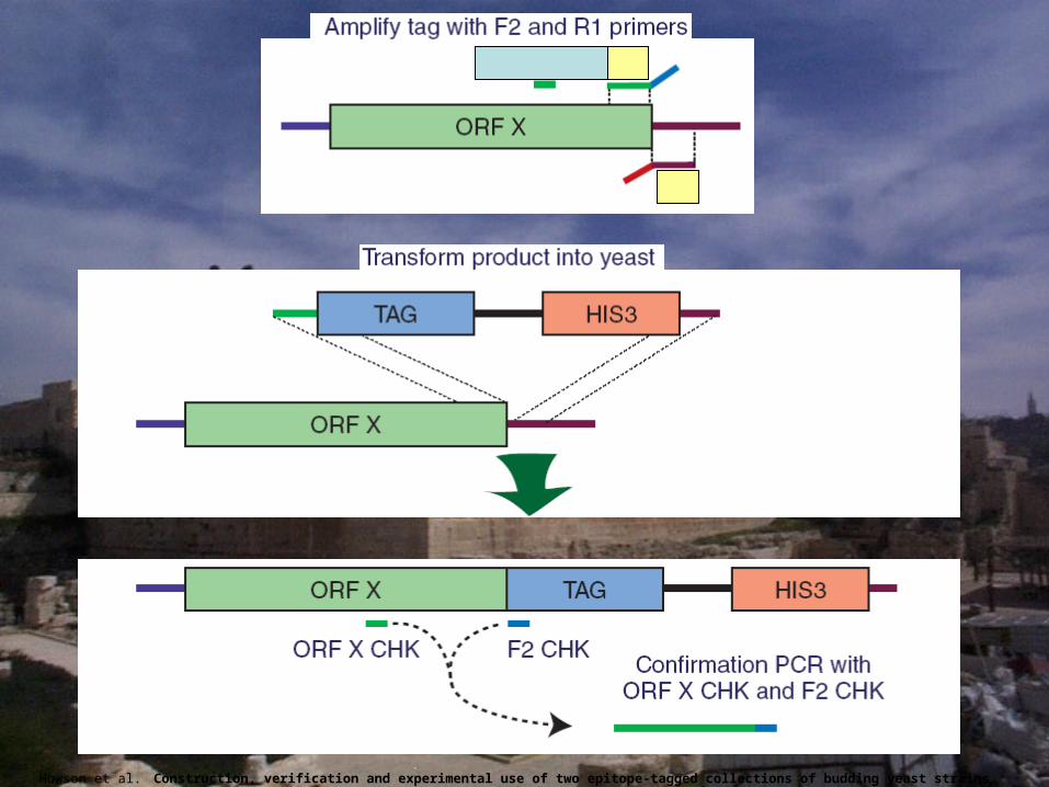
Howson et al. Construction, verification and experimental use of two epitope-tagged collections of budding yeast strains Comp Funct Genom 2005; 6: 2–16.

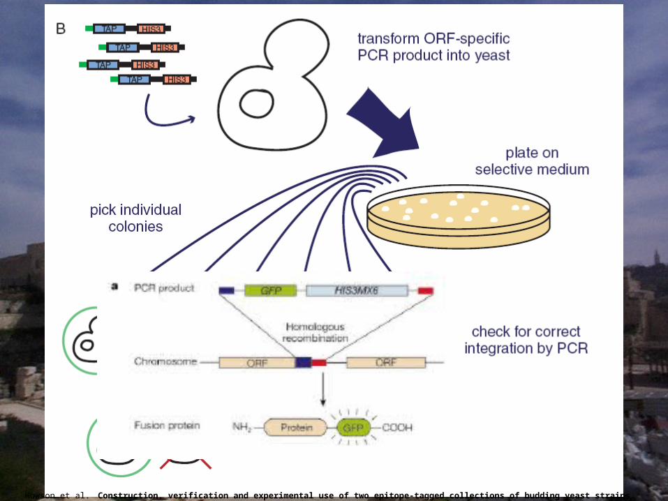
Howson et al. Construction, verification and experimental use of two epitope-tagged collections of budding yeast strains Comp Funct Genom 2005; 6: 2–16.

Localization determination

• Micrographs of each strain lacking ORF name were evaluated independently by two scorers.

• Initial classification of each protein to one or more of 12 subcellular localization categories

• Refinement by co-localization

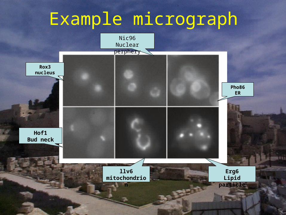
Rox3nucleus

llv6mitochondrion

Hof1Bud neck

Erg6Lipid particle

Pho86ER

Nic96Nuclear perphery

Example micrograph

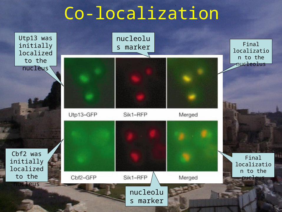
Co-localization

Final localization to the nucleolus

Final localization to the nucleus

nucleolus marker

nucleolus marker

Cbf2 was initially

localized to the nucleus

Utp13 was initially

localized to the nucleus

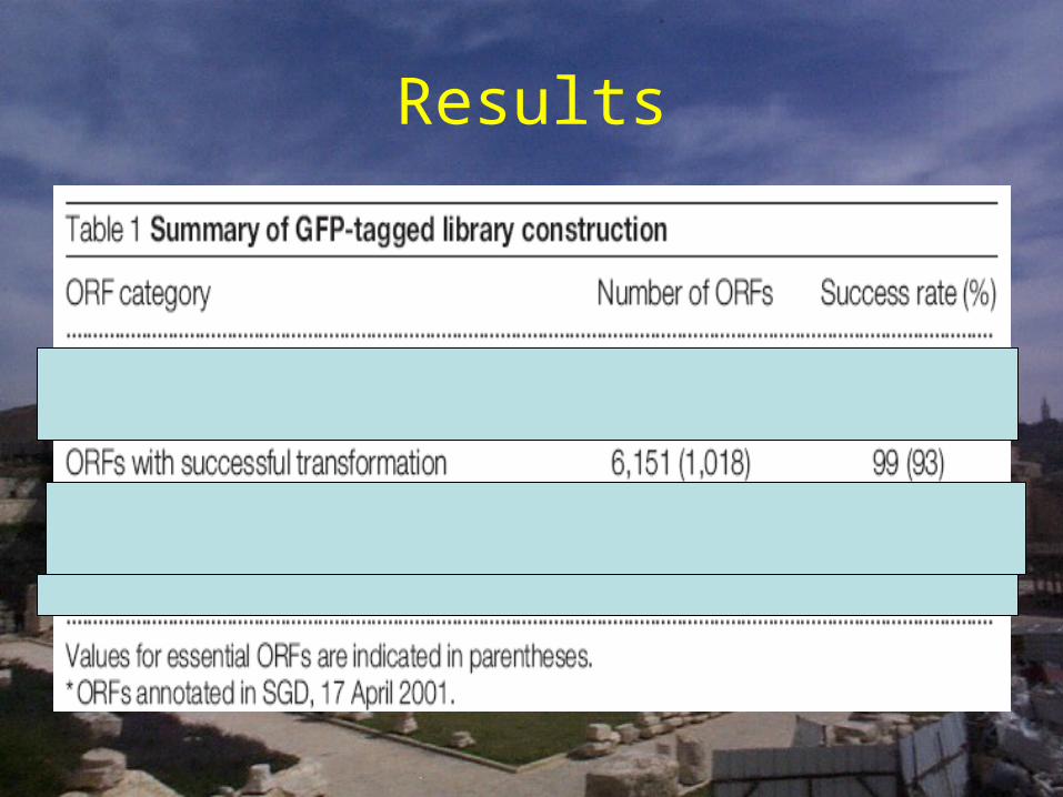
Results

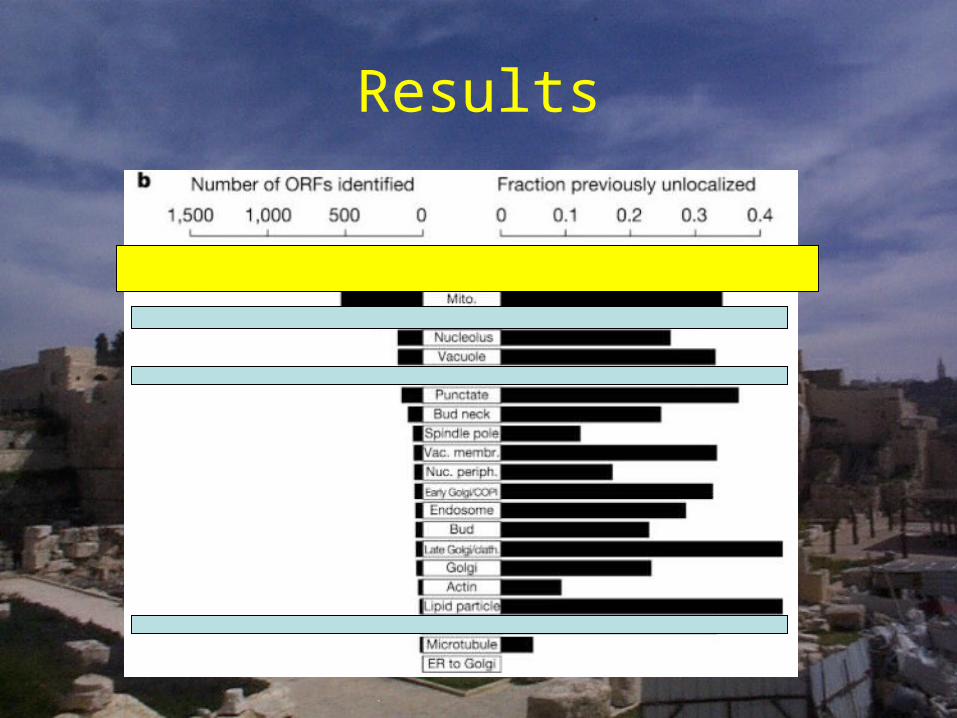
Results

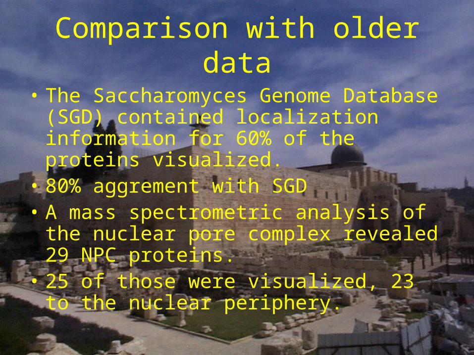
Comparison with older data

• The Saccharomyces Genome Database (SGD) contained localization information for 60% of the proteins visualized.

• 80% aggrement with SGD • A mass spectrometric analysis of the

nuclear pore complex revealed 29 NPC proteins.

• 25 of those were visualized, 23 to the nuclear periphery.

Localization and interaction

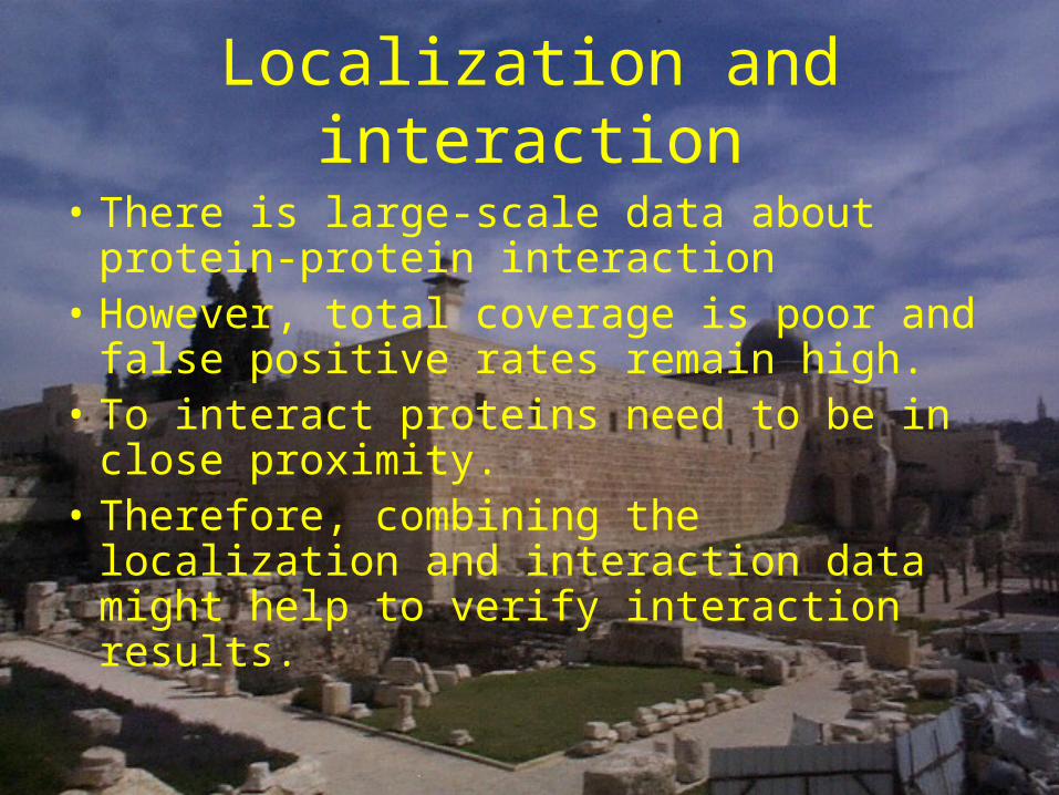
• There is large-scale data about protein-protein interaction

• However, total coverage is poor and false positive rates remain high.

• To interact proteins need to be in close proximity.

• Therefore, combining the localization and interaction data might help to verify interaction results.

Localization and interaction

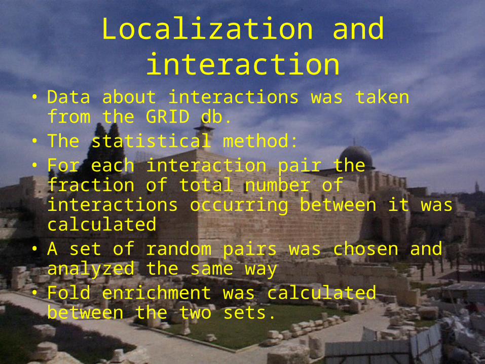
• Data about interactions was taken from the GRID db.

• The statistical method:• For each interaction pair the fraction of total

number of interactions occurring between it was calculated

• A set of random pairs was chosen and analyzed the same way

• Fold enrichment was calculated between the two sets.

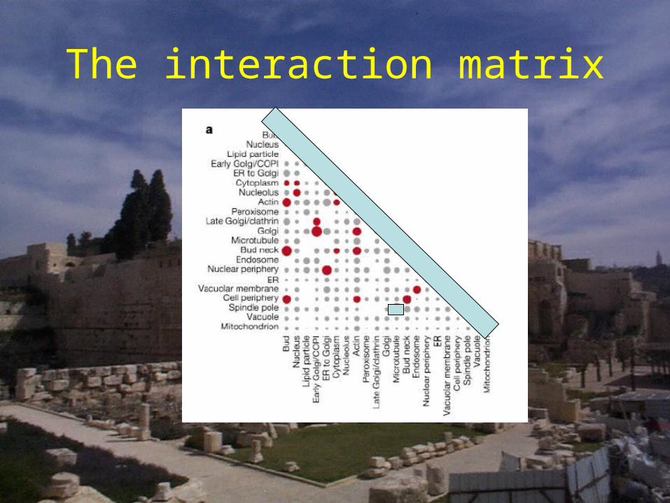
The interaction matrix

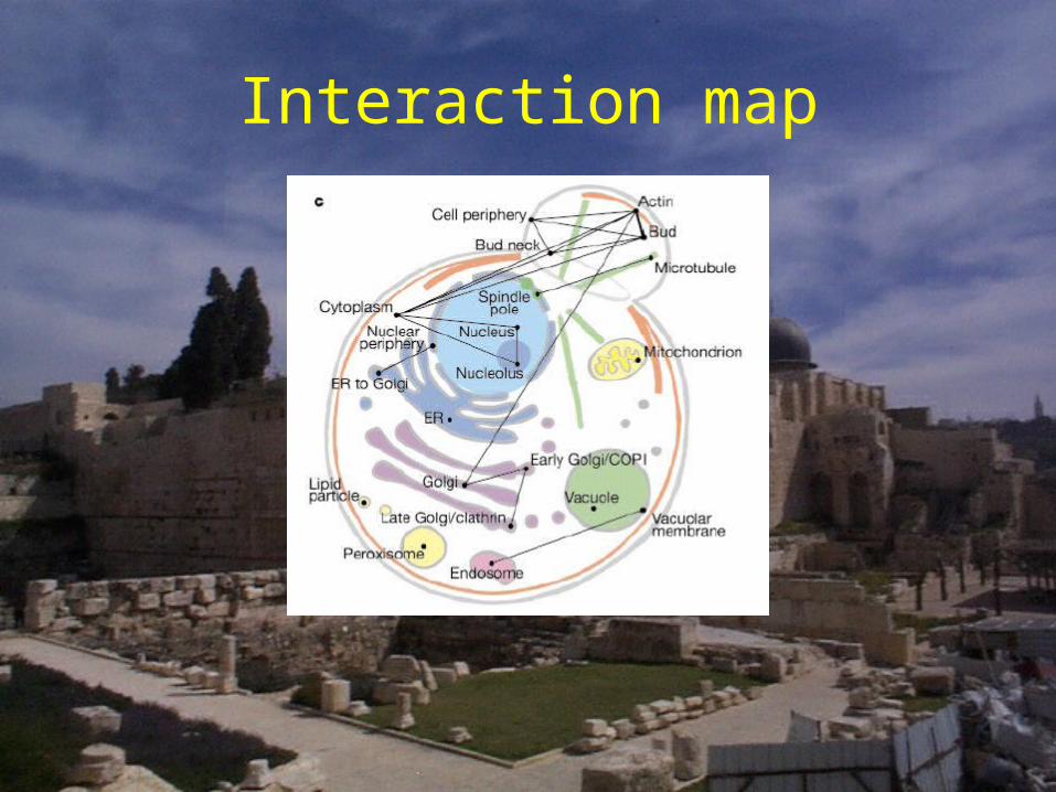
Interaction map

problems

• Possible destruction of localization signals

• Possible Interruption of post translational modifications

• Fusion proteins might have steric hindrance

Summary

• Localization data for many previously unlocalized proteins was collected.

• Agreement with older data.

• Identification of interacting compartments.

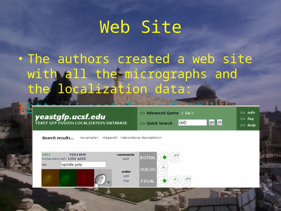
Web Site

• The authors created a web site with all the micrographs and the localization data:

• http://yeastgfp.ucsf.edu/

Global analysis of proteinexpression in yeast

Ghaemmaghami S. et. al. nature 425 (October 2003)

• Goal: to globally determine protein expression levels in the infamous budding yeast.

• Identification of mis-annotated genes

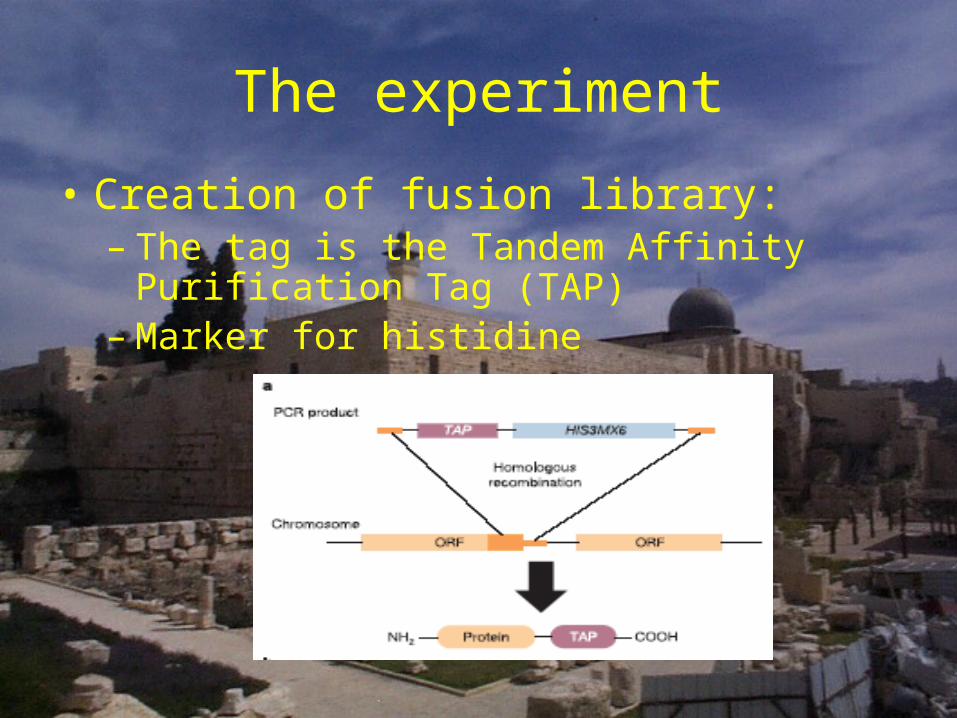
The experiment

• Creation of fusion library:– The tag is the Tandem Affinity Purification Tag

(TAP)– Marker for histidine

The experiment

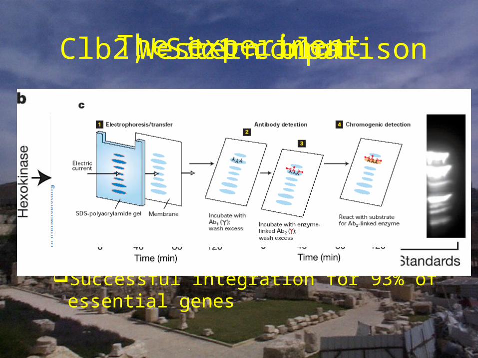
• Checking that the proteins are fused and are activeWestern blot analysis.Clb2, Sic 1 comparison.Successful integration for 98% of ORF’s

annotated in the Sacchromyces DB.Successful integration for 93% of essential

genes

Western blotClb2, Sic1 comparison

Results

• Detected 79 % of essential ORF’s.

• 83 % of ORF’s with assigned gene names

• Identified Protein product for 1,018 functionally uncharacterized ORF’s

• 73 % of all annotated ORF’s– Sporious ORF’s– Genes encoding for product not needed in log

phase

Eliminating spurious ORF’s

• Product not identified both by GFP & TAP.

• CEC values below an arbitary cut-off.

Codon Enrichment Correlation

• Codon usage in genuine coding regions deviates systematically from randomly generated ORF’s– Preference in amino acid composition– Bias in the usage of synonymous codons

• The CEC evaluates the pattern of codon usage in potential ORF’s

CEC

• Calculation of CEC:

• The prevalence of each codon in the 3,753 named ORF’s was calculated.

• The prevalance of each codon in a random sequence was calculated as well.

• The enrichment of each codon :Prevelance in Positive set

Prevalance in random set

CEC

• The enrichment was calculated in the same way for each test ORF

• The CEC is the linear correlation coefficient between the test ORF and the positive set

• They could have calculated P-values instead.

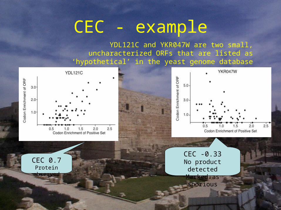
CEC - exampleYDL121C and YKR047W are two small, uncharacterized ORFs

that are listed as ‘hypothetical’ in the yeast genome database

CEC 0.7Protein observed

CEC -0.33No product detectedMarked as sporious

Remember kellis?

Dedicated to Nir & Sonia

Sequencing and comparison of yeast species to identify genes and

regulatory elements(*)

Mannollis Kellisחוקר ראשי: •Eric s. Landerראש מעבדה: •

(*) Kellis M, et al. (2003) Sequencing and comparison of yeast species to identify genes and regulatory elements. Nature 423: 241–254

Remember Kellis?

• Kellis identified 496 sporious ORF’s

• 489 of those were not observed in this study.

• 381 sporious ORF’s that this study identified overlap with Kellis.

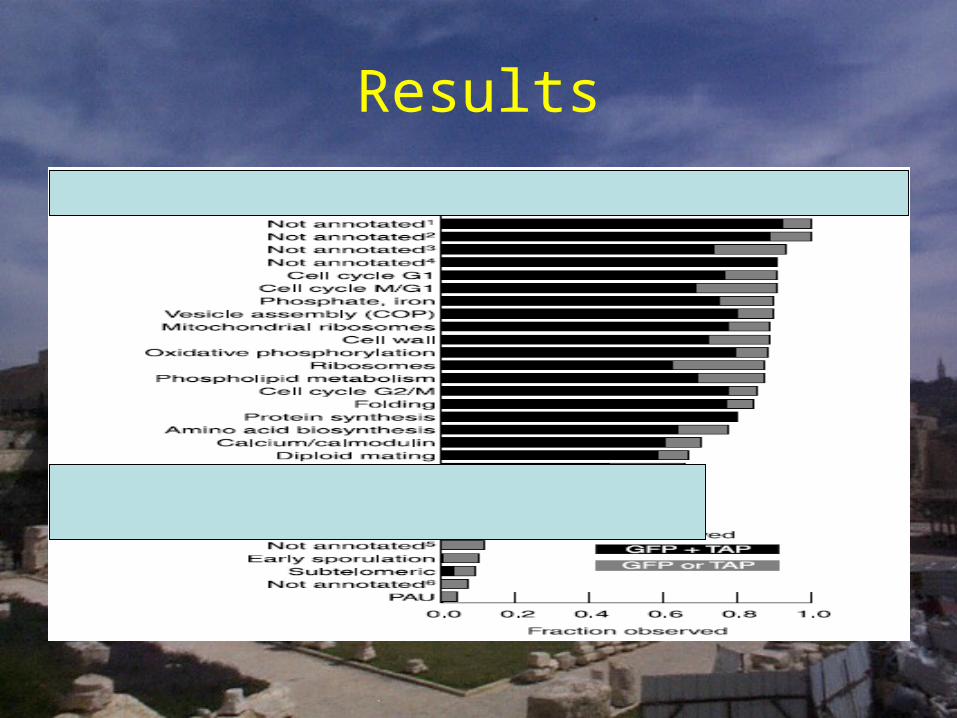
Results

Results

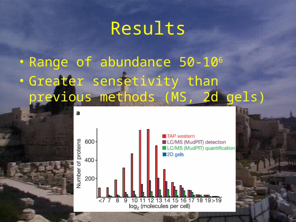
• Range of abundance 50-106

• Greater sensetivity than previous methods (MS, 2d gels)

Results

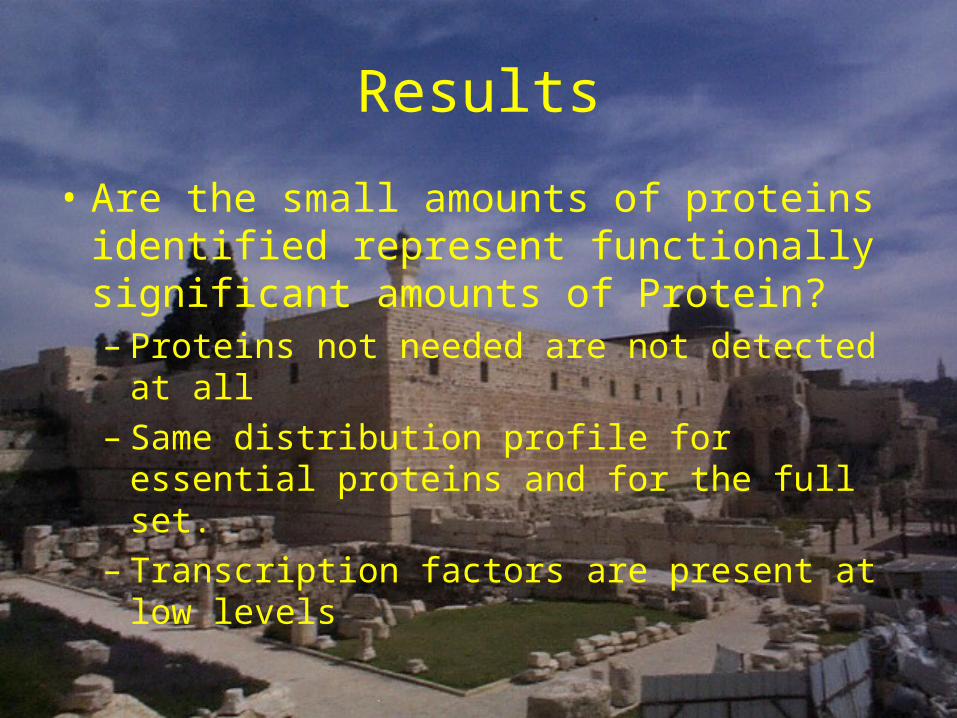
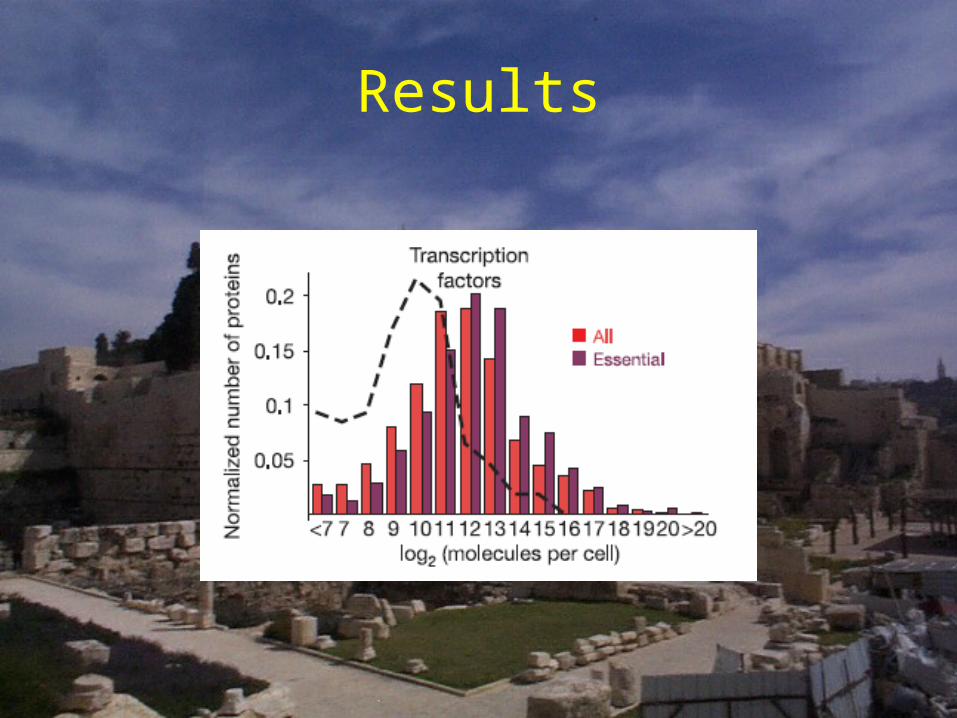
• Are the small amounts of proteins identified represent functionally significant amounts of Protein?– Proteins not needed are not detected at all– Same distribution profile for essential proteins

and for the full set. – Transcription factors are present at low levels

Results

mRNA - Protein

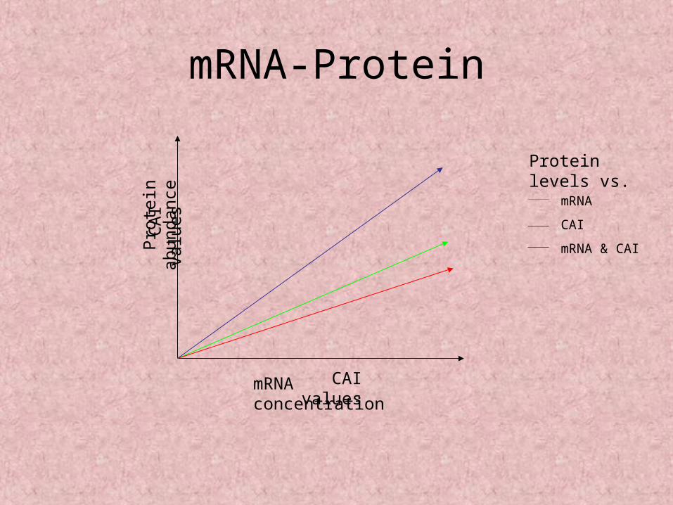
• Observed a significant relationship between mRNA levels1 to Protein levels(rs=0.57)

• The Codon Adaptation Index is used to measure the composition of codons in a given ORF in comparison with a predefined set of reference genes.

• Higher CAI values usually mean faster translation.

• Relationship also between protein abundance and CAI values (rs=0.55)

1. Holstege, F. C. et al. Dissecting the regulatory circuitry of a eukaryotic genome. Cell 95, 717–728 (1998).

mRNA-Protein

mRNA concentration

Pro

tein

ab

unda

nce

CAI values

CA

I va

lues

mRNA

CAI

mRNA & CAI

Protein levels vs.

Summary

• The research demonstrated the possibility to globally determine Protein abundances.

• The results show a great variation in expression level between proteins.

• The method also helps in the identification of spurious ORF’s

Post transcriptional expression regulation in the yeast Saccharomyces cerevisiae on a genomic scale

Beyer et. al.Molecular & Cellular Proteomics 3.11

• Goal: to invesigate the relation of transcription, translation and protein turnover on a genomic scale.

Motivation

• To make use of the large scale data to create a more complete picture of the cell’s strategy in determining expression profiles of proteins

Source Data

• mRNA abundance data from 36 experiments

• 30 independent measurements for > 6000 ORF’s

• The data was normalized to reduce inconsistencies between the data sets.

• Resulting dataset characterized with low noise

Source Data

• Protein abundance data from Previous article and from Greenbaum D et. al. Comparing protein abundance and mRNA expression levels on a genomic scale. Genome Biol. 4, 117.1-117.8

• Only 1,669 ORF’s are contained in both studies.• Therefore, protein abundances are much less

certain than mRNA abundances.• However, when using the average the

correlation between Protein and mRNA levels are most significant.

• With new data the correlations will improve.

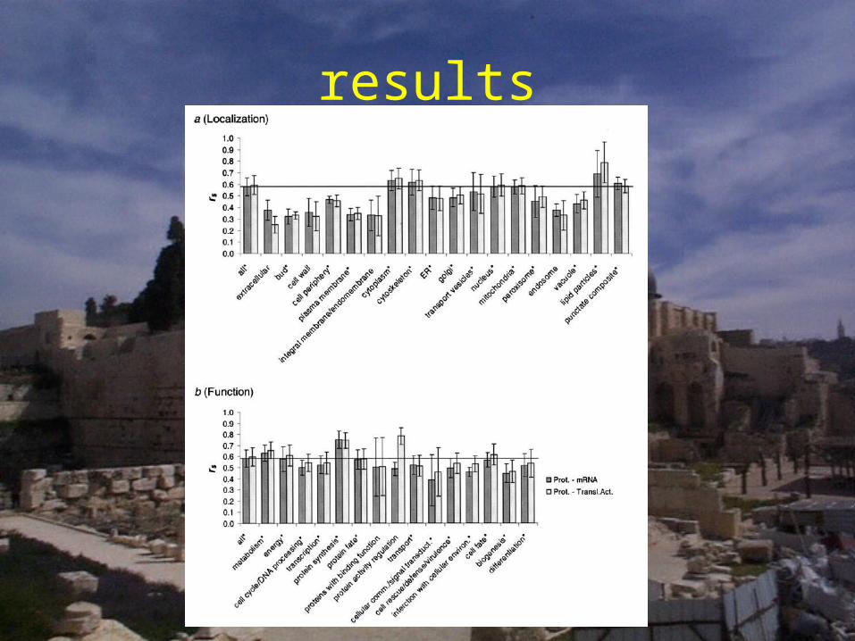
Results

• Protein – mRNA abundance• The median value for the entire cell

– Protein 2,800– mRNA 0.7

• Median values are less affected by extreme values

• Median is more stable against variations between the studies.

• The correlation discovered was rs=0.58.

Source Data

• Trying to make a better model.• Adding two more values which determine the

translation rate • Ribosome occupancy – the fraction of mRNA

bound to ribosomes• Ribosome density – how many ribosomes are on

one mRNA• Translational rate – Ribosome density * Ribosome occupancy• Translational activity – mRNA levels * Translational rate

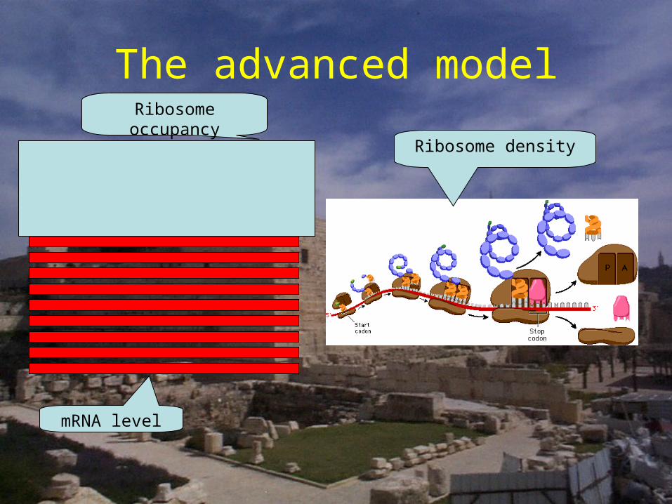
The advanced model

mRNA level

Ribosome occupancy

Ribosome density

results

Results

• Spearman rank correlation coefficents were taken between mRNA abundance and Protein abundance and between Translational activity and protein abundance

• The rs improved only to 0.596

Results

• Protein to mRNA ratio is indicative of post transcriptional regulation as well as to translational activity

• The turnover rate of proteins has a significant affect on Protein-mRNA ratios

• The Protein Half-life Descriptor (PHD)

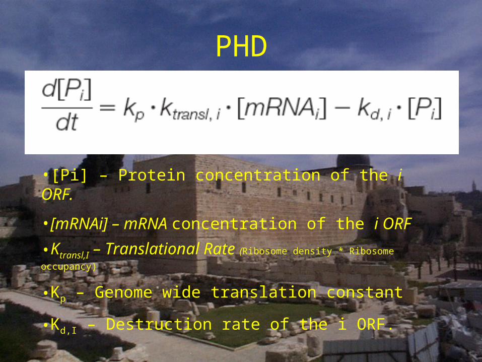
PHD

•[Pi] – Protein concentration of the i ORF.

•[mRNAi] – mRNA concentration of the i ORF

•Ktransl,I – Translational Rate (Ribosome density * Ribosome occupancy)

•Kp – Genome wide translation constant

•Kd,I – Destruction rate of the i ORF.

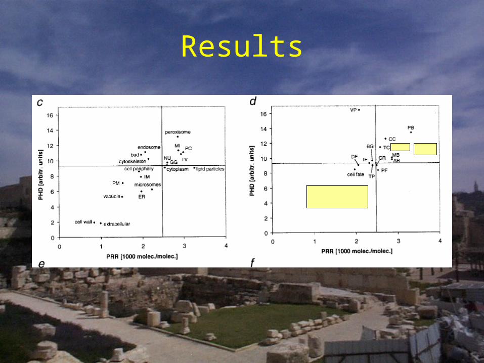
Results

Problems

• The data about protein abundance is much less accurate than the mRNA data

• As well as the data for ribosome density, occupancy and for transcript length.

• The calculation of ribosome density was done with relation to transcript length.

• PHD calculations are based on measurements from different labs, where growth conditions might not be identical.

Advantages

• Opens a new way of analyzing the cell’s activity.

• With more data which is sure to come, the measuerments will be more accurate.

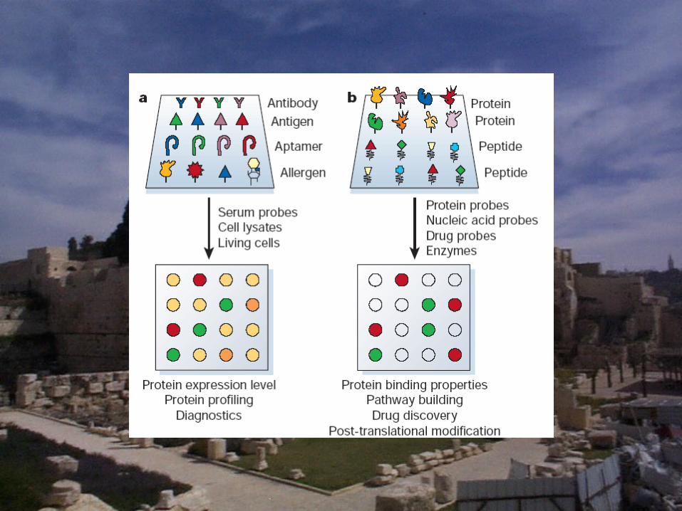
Protein Microarray

• Functional –individually purified proteins are spotted on a surface and analyzed for activity

• Analytical – protein specific ligands are spooted on the surface and are used to monitor levels of proteins

Microarray pros & cons

• Pros:– Direct identification of protein.– Identification of multiple positives.– automation

• Cons:– Proteins are not in their natural environment– Requires individual growth and purification of each

protein– Proteins may not fold correctly or may take only one

isoform.

“Going from sequence to Going from sequence to consequence is of course what consequence is of course what proteomicsproteomics is all about.” is all about.”

Greg PetskoGreg PetskoC & E News, November 26 (2001C & E News, November 26 (2001))