Labor Productivity and Employment Gaps in Sub · PDF fileLabor Productivity and Employment Gaps in ... This paper is a product of the “Agriculture in Africa—Telling Facts from

Policy Research Working Paper 7234

Labor Productivity and Employment Gaps in Sub-Saharan Africa

Ellen B. McCullough

Africa RegionOffice of the Chief EconomistApril 2015

WPS7234P

ublic

Dis

clos

ure

Aut

horiz

edP

ublic

Dis

clos

ure

Aut

horiz

edP

ublic

Dis

clos

ure

Aut

horiz

edP

ublic

Dis

clos

ure

Aut

horiz

ed

Produced by the Research Support Team

Abstract

The Policy Research Working Paper Series disseminates the findings of work in progress to encourage the exchange of ideas about development issues. An objective of the series is to get the findings out quickly, even if the presentations are less than fully polished. The papers carry the names of the authors and should be cited accordingly. The findings, interpretations, and conclusions expressed in this paper are entirely those of the authors. They do not necessarily represent the views of the International Bank for Reconstruction and Development/World Bank and its affiliated organizations, or those of the Executive Directors of the World Bank or the governments they represent.

Policy Research Working Paper 7234

This paper is a product of the “Agriculture in Africa—Telling Facts from Myths” project managed by the Office of the Chief Economist, Africa Region of the World Bank, in collaboration with the Poverty and Inequality Unit, Development Economics Department of the World Bank, the African Development Bank, the Alliance for a Green Revolution in Africa, Cornell University, Food and Agriculture Organization, Maastricht School of Management, Trento University, University of Pretoria, and the University of Rome Tor Vergata. It is part of a larger effort by the World Bank to provide open access to its research and make a contribution to development policy discussions around the world. Policy Research Working Papers are also posted on the Web at http://econ.worldbank.org. The author of the paper may be contacted at [email protected].

Drawing on a new set of nationally representative, interna-tionally comparable household surveys, this paper provides an overview of key features of structural transformation—labor allocation and labor productivity—in four African economies. New, micro-based measures of sector labor allo-cation and cross-sector productivity differentials describe the incentives households face when allocating their labor. These measures are similar to national accounts-based measures that are typically used to characterize structural changes in African economies. However, because agricultural workers

supply far fewer hours of labor per year than do workers in other sectors, productivity gaps disappear almost entirely when expressed on a per-hour basis. What look like large productivity gaps in national accounts data could really be employment gaps, calling into question the prospective gains that laborers can achieve through structural trans-formation. These employment gaps, along with the strong linkages observed between rural non-farm activities and primary agricultural production, highlight agriculture’s con-tinued relevance to structural change in Sub-Saharan Africa.

Labor Productivity and Employment Gaps in Sub-Saharan Africa

Ellen B. McCullough

Charles H. Dyson School of Applied Economics and Management Cornell University

*Author email: [email protected]

JEL: J21, J22, J24, O12, Q10, Q12

Keywords: Structural transformation; Sub-Saharan Africa; Agricultural labor productivity; Sector labor shares; Productivity gaps.

Acknowledgements

I am grateful for the extraordinary effort by the LSMS-ISA team of the World Bank to collect the innovative data sets used in this analysis, under the leadership of Gero Carletto and with funding from the Bill & Melinda Gates Foundation. Each country’s National Statistics Office, including survey supervisors and enumerators, played a central role in implementing large scale, high quality, nationally representative surveys. And, of course, many respondents across Sub-Saharan Africa were very generous with their time. My time was funded through the Food

Systems and Poverty Reduction IGERT traineeship of the National Science Foundation. Additionally, support from the Agriculture in Africa: Telling Facts from Myths project, led by the World Bank with cofounding from the African Development Bank, is gratefully acknowledged. I especially thank Chris Barrett for providing overall guidance and Megan Sheahan for research support. I would like to thank the entire “Myths and Facts” team, in particular Luc Christiaensen for his leadership and Amparo Palacios-Lopez for reducing the transactions costs of data use. For valuable comments on this manuscript and its earlier iterations, I thank Paul Christian, Brian Dillon, Walter Falcon, Bob Herdt, Linden McBride, John Nash, Prabhu Pingali, Abebe Shimeles, Erik Thorbecke, and members of Chris Barrett’s research group. Any remaining errors are mine alone.

1

1. Introduction

Structural change is integral to economic development. In the development context, it refers both to the reallocation of labor from one low-productivity sector to another, higher-productivity sector, and to the economic growth resulting from this shift. Structural change is a dynamic process powered by several key features – productivity levels within sectors, productivity gaps between them, and the movement of labor from low productivity to high productivity sector(s). In poor economies, agriculture is typically the sector that employs the most people and uses labor least productively. Therefore, structural change is tightly associated with the exit of labor from agriculture to other sectors of the economy (Timmer 1988). The larger the productivity gap between agriculture and other sectors, the larger the opportunity to achieve growth through structural change. Over time, cross-sector productivity gaps tend to shrink, as factor market integration gradually equalizes returns to labor across sectors. However, productivity gaps generally do not disappear altogether, and small labor productivity gaps between agriculture and other sectors persist even in high income countries (Lele, Agarwal, and Goswami 2013).

Growth in labor productivity, overall and within agriculture, has been a strong predictor of poverty reduction because of the important linkages between wages, household self-employment, and the real incomes of the poor. Though land productivity growth typically precedes labor productivity growth, the process of agricultural development is thought to begin when output per agricultural worker increases (Timmer 1988). Agricultural labor productivity growth is particularly important because of the direct effects on the many workers who participate in the agricultural sector, and also because it causes growth in other sectors (De Janvry and Sadoulet 2009). Agricultural growth also plays a role in lowering agricultural employment shares. Through farmer income effects, agricultural productivity growth stimulates rural demand for non-agricultural non-tradable goods and services, pushing up wages outside of agriculture and pulling workers out of the sector (McMillan and Harttgen 2014). Historically, agricultural growth has been shown to contribute more to poverty reduction than non-agricultural growth (Christiaensen, Demery, and Kuhl 2011).

1.1 Relevant Literature

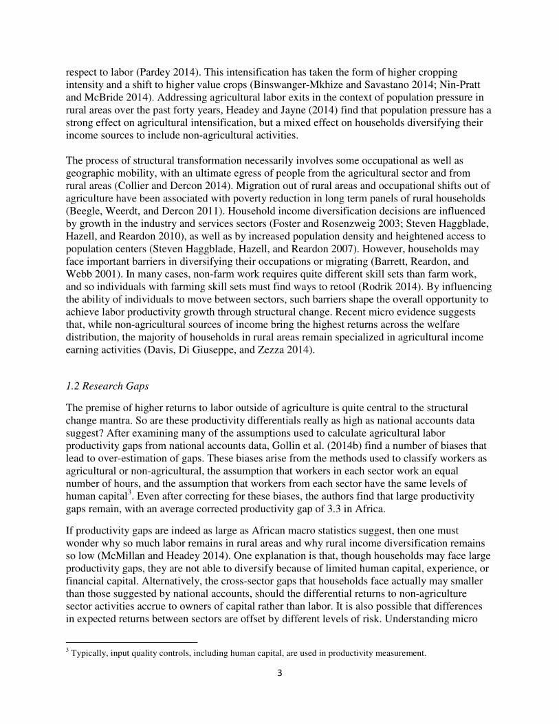
This paper focuses on Sub-Saharan Africa, the region with the lowest per capita incomes, largest shares of value added captured by agriculture, largest shares of the work force employed in agriculture, and lowest agricultural labor productivity (Figure 1a) (World Bank Group 2014). According to national accounts data, labor in developing countries is 4.5 times more productive outside of agriculture than in it. In middle income countries, the ratio is 3.4, and in high income countries, it is 2.2. Within African countries, non-agricultural labor is 6 times more productive outside of agriculture than in it2 (Figure 1b) (Gollin, Lagakos, and Waugh 2014b). Other recent assessments of productivity gaps confirm that large cross-sector productivity differentials persist in Sub-Saharan African countries (McMillan and Harttgen 2014; Lele, Agarwal, and Goswami 2013).

2 These ratios were calculated using data Gollin et al. (2014a) and World Bank classifications of countries by

income.

2

Labor productivity in an economy can be improved either within sectors (e.g. through technological gains and capital accumulation) or structurally (e.g. by shifting labor out of less-productive activities and into more-productive activities). During the 1990s, African labor entered agriculture rather than exiting it, thereby suppressing overall labor productivity growth (McMillan and Rodrik 2011). Since 2000, labor productivity growth within agriculture has accelerated in Eastern and Southern Africa, and in Nigeria (Pardey 2014; Block 2013). Decomposition of recent labor productivity growth trends suggests that labor exits from agriculture explain about half of recent overall labor productivity growth across Africa (McMillan and Harttgen 2014; McMillan, Rodrik, and Verduzco 2014). These recent favorable trends are also reflected in national accounts and per capita consumption data, and have become known as the “African growth miracle” (e.g., Young 2012). From a structural change perspective, Sub-Saharan Africa still lags behind other regions of the world. Nevertheless, African countries seem to be following the same patterns of agricultural labor exits as those previously followed by countries in other regions (McMillan and Harttgen 2014). However, African structural change pathways differ from those in Asia and Latin America in that the services sector, which is characterized by relatively low productivity in African countries, has been a primary recipient of labor exiting from agriculture (Rodrik 2014). In other regions, industrialization has been core to the structural change process. High levels of informality in the industry and services sectors has lowered their average productivity and suppressed the gains to be exploited from agricultural exits. In Vietnam, important productivity gains resulted not only by shifting labor out of agriculture, but also by shifting labor into formal, higher-productivity firms within the industrial sector (McCaig and Pavcnik 2013). Because agricultural labor shares are still so large in African countries, the potential gains from reallocating labor to higher-productivity sectors is believed to be very high (McMillan and Headey 2014). A large initial agricultural labor share, rising female education, rising commodity prices, good governance, and agricultural productivity growth all appear to be positively correlated with labor exits from agriculture (McMillan and Harttgen 2014). Poor market infrastructure, heterogeneous and difficult agroclimatic conditions, and generally unfavorable policy enabling environments all pose challenges to labor productivity growth in African agriculture. Nevertheless, in the many African economies that are landlocked and poor in natural resources, agricultural labor productivity growth probably provides the only pathway towards economic growth and poverty reduction (Dercon 2009). Labor is one of several important factors in agricultural production, which also relies on land, capital, and other inputs. Intensification of agricultural labor use can be driven by land scarcity (e.g., high population pressure) or by capital scarcity (e.g., high interest rates). Historically, growing population pressure has been associated with more intensive agricultural systems characterized by reduced frequency and length of fallow periods on agricultural land (Ruthenberg 1971; Pingali, Bigot, and Binswanger 1987). Intensive systems typically use higher labor inputs per unit of land for tasks such as land preparation, soil fertility management, water management, weeding, harvesting, and long term improvements in land quality. In aggregate, agricultural labor productivity grew slower than agricultural land productivity between 1961 and 2010 in Africa, which implies some intensification of African agriculture with

3

respect to labor (Pardey 2014). This intensification has taken the form of higher cropping intensity and a shift to higher value crops (Binswanger-Mkhize and Savastano 2014; Nin-Pratt and McBride 2014). Addressing agricultural labor exits in the context of population pressure in rural areas over the past forty years, Headey and Jayne (2014) find that population pressure has a strong effect on agricultural intensification, but a mixed effect on households diversifying their income sources to include non-agricultural activities. The process of structural transformation necessarily involves some occupational as well as geographic mobility, with an ultimate egress of people from the agricultural sector and from rural areas (Collier and Dercon 2014). Migration out of rural areas and occupational shifts out of agriculture have been associated with poverty reduction in long term panels of rural households (Beegle, Weerdt, and Dercon 2011). Household income diversification decisions are influenced by growth in the industry and services sectors (Foster and Rosenzweig 2003; Steven Haggblade, Hazell, and Reardon 2010), as well as by increased population density and heightened access to population centers (Steven Haggblade, Hazell, and Reardon 2007). However, households may face important barriers in diversifying their occupations or migrating (Barrett, Reardon, and Webb 2001). In many cases, non-farm work requires quite different skill sets than farm work, and so individuals with farming skill sets must find ways to retool (Rodrik 2014). By influencing the ability of individuals to move between sectors, such barriers shape the overall opportunity to achieve labor productivity growth through structural change. Recent micro evidence suggests that, while non-agricultural sources of income bring the highest returns across the welfare distribution, the majority of households in rural areas remain specialized in agricultural income earning activities (Davis, Di Giuseppe, and Zezza 2014).

1.2 Research Gaps

The premise of higher returns to labor outside of agriculture is quite central to the structural change mantra. So are these productivity differentials really as high as national accounts data suggest? After examining many of the assumptions used to calculate agricultural labor productivity gaps from national accounts data, Gollin et al. (2014b) find a number of biases that lead to over-estimation of gaps. These biases arise from the methods used to classify workers as agricultural or non-agricultural, the assumption that workers in each sector work an equal number of hours, and the assumption that workers from each sector have the same levels of human capital3. Even after correcting for these biases, the authors find that large productivity gaps remain, with an average corrected productivity gap of 3.3 in Africa.

If productivity gaps are indeed as large as African macro statistics suggest, then one must wonder why so much labor remains in rural areas and why rural income diversification remains so low (McMillan and Headey 2014). One explanation is that, though households may face large productivity gaps, they are not able to diversify because of limited human capital, experience, or financial capital. Alternatively, the cross-sector gaps that households face actually may smaller than those suggested by national accounts, should the differential returns to non-agriculture sector activities accrue to owners of capital rather than labor. It is also possible that differences in expected returns between sectors are offset by different levels of risk. Understanding micro

3 Typically, input quality controls, including human capital, are used in productivity measurement.

4

level cross-sector productivity differences, and how they relate to sector allocation decisions, is crucial for understanding the forces that power agricultural labor exits.

I use a new micro-level dataset to measure key structural change parameters – sector participation, time use, and labor productivity – from a micro perspective. This paper draws on the Integrated Surveys on Agriculture from the Living Standards Measurement Study group at the World Bank (LSMS-ISA datasets), which explicitly collect information about respondents’ time use across sectors. Particular attention is paid to farm labor, which is often neglected in large scale, multi-topic surveys because of the challenges involved in collecting detailed agricultural data. The analysis currently includes surveys from Ethiopia, Malawi, Tanzania and Uganda. The countries that comprise the LSMS-ISA dataset exhibit considerable heterogeneity with respect to GDP per capita, share of agriculture in the labor force, share of agriculture in the economy, and productivity gaps (Figure 1).

The micro perspective is quite relevant for this study for several reasons. First, it reflects the perspective of individuals and firm owners making labor allocation decisions in developing countries. Second, micro datasets contain the variables required to examine the assumptions on which macro statistics are generated. Third, micro datasets allow for productivity measures to be paired with relevant covariates of labor allocation decisions at the household and individual levels. This kind of micro perspective is largely absent from the literature about structural change in African economies. Demographic and Health Survey (DHS) datasets, also micro datasets, are sometimes used to calculate sector labor shares, as an alternative to measures based on population censuses or national accounts (e.g., McMillan and Harttgen 2014; McMillan and Rodrik 2011). While DHS surveys have very extensive coverage, they cannot be used to generate measures of time use or returns to sector participation.

I generate micro measures of sector participation shares that are fairly close to those in national accounts datasets. Microeconomic analogs of sector productivity and cross-sector productivity gaps based on output per sector participant per year are smaller than those generated from national accounts data but fairly close to the corrected gaps generated by Gollin et al. (2014b). However, micro measures of agricultural labor shares based on time use are much smaller than participation measures because participants tend to work fewer hours in agriculture than in other sectors. Consequently, measures of cross-sector productivity gaps disappear almost entirely when they are based on time inputs by sector workers. Cross-sector productivity gaps observed in national accounts data, therefore, may reflect gaps in employment levels rather than gaps in the returns to hours worked between sectors. These results suggest that the forces pulling labor into non-agriculture sectors may be weaker than many believe them to be. Because time inputs in agriculture are generally low, possibly due to biophysical constraints, there still exists an opportunity to achieve growth in annual output per worker by increasing labor supply to the industry and services sectors.

2. Data and Variable Construction

To examine labor productivity gaps from a micro-economic perspective, I generate labor productivity measures and other key variables from the Living Standards Measurement Survey – Integrated Surveys in Agriculture (LSMS-ISA) dataset. I draw on a cross-section of the most recent LSMS-ISA datasets available, comprised of the Ethiopia Rural Socioeconomic Survey

5

(2011-12), the Malawi Integrated Household Survey (2010-11), the Tanzania National Panel

Survey (2010-11), and the Uganda National Panel Survey (2010-11). LSMS-ISA surveys were implemented by each country’s national statistics office, with technical support from the World Bank Development Economics Research Group. These datasets are nationally representative, including urban and rural households regardless of occupation or sector of employment. Rural and urban areas are defined by each country’s statistics office. Unlike the other surveys, the Ethiopian dataset is representative of rural areas and small towns and excludes urban areas. Table 1 depicts the basic characteristics the datasets used in this study. In the paper, “small town” results for Ethiopia are represented as “urban”, “rural” as “rural”, and full sample results as “all”. It is worth emphasizing the novelty of LSMS-ISA datasets. Surveys of farming populations often collect detailed plot-level farm management information similar to the LSMS-ISA surveys, but they do not also include information on time use off the farm, and generally do not sample non-farming households. The multi-topic, multi-purpose LSMS-ISA questionnaire includes questions on labor market participation, labor inputs into in household farm and non-farm enterprises, and returns to enterprises and labor market participation. They are also internationally comparable to some extent, allowing for cross-country comparisons. Using the LSMS-ISA data, I construct individual level, annualized labor supply aggregates for three types of activities – household operated farm enterprises (farms), household operated nonfarm enterprises (NFEs), and wage labor market participation. Labor supply recall questions differ in the LSMS-ISA surveys by type of activity. Appendix A contains detailed information about the construction of all of the variables used in this analysis. Wage labor supply variables are generated over a twelve month recall period from individuals’ reported number of months worked over the last year, typical number of weeks worked per month, and typical number of hours worked per week. In the agriculture modules of the surveys, labor inputs by individual household members are collected for each farm plot. These inputs are aggregated for each household member to generate the annual own farm labor supply variable. For non-farm enterprises, participation by household members is flagged at the firm level. Different approaches to collecting NFE labor supply are followed in different countries. These are detailed in Table A.3 in the appendix. Systematic measurement error in construction of labor supply variables is particularly concerning, should respondents recall different types of activities with different errors. Differences in recall period (through questionnaire design or timing of interview) or differences in recall ability for different activities (e.g., rare, “salient” events vs. common ones) can lead to differences in household responses (Beegle, Carletto, and Himelein 2012; Bound, Brown, and Mathiowetz 2001). The possibility of measurement error in the constructed labor supply aggregates is addressed in section 5 of this paper. Next, I construct aggregates of labor demand by household operated farms and NFEs, which include hired labor in addition to labor supplied by family members. Of interest are both the number of firm workers and the labor inputs supplied by workers to each firm. In the case of farm enterprises, we have a good measure of labor inputs and the number of household members who work on the farm and the total number of hours worked by household members and hired workers, but we do not observe the number of employees hired. In the case of NFEs, we

6

universally observe the number of hired workers but not the hours that they supply to the firm. It is quite common for farm households to hire in labor (between 30 % and 94 % of farms do it), but less so for non-farm enterprises (in all cases, fewer than 19% of households operating an enterprise hire in any workers). Returns to labor market participation are comprised of the gross total wages received by wage workers, including in-kind payments (e.g., meals received) and gratuities. Costs of participating in wage labor markets are not measured so it is not possible to construct a net revenue measure. The returns to operating a farm enterprise are based on net farm revenue, which is analogous with the “value added” concept that underlies national accounts data. The net value of farm output is derived from the Rural Income Generating Activities (RIGA) calculations and includes the value of own-consumed farm output as measured through the consumption module (Davis et al. 2010). For non-farm enterprises, reported enterprise profit is considered a more reliable measure of net firm revenue than a constructed measure based on gross revenues minus costs (de Mel, McKenzie, and Woodruff 2009). Where available, I construct the annualized net firm revenue variable using reported profits. Otherwise, I use household estimates of gross NFE revenue and costs. To facilitate cross-country comparison, all measures of returns are converted to constant international dollars using the purchasing power parity conversion factor for private consumption from the World Bank’s World Development Indicators. Using the labor supply variables and the returns variables, I construct average labor productivity variables. These are done separately for the three types of activities – wage labor, farms, and NFEs – as a simple ratio between returns to an activity and labor inputs into the activity. Two types of average labor productivity measures are constructed. The per-worker measure is based on output per worker per year. The per-hour measure is based on output per hour of labor supplied to each activity per year. Because we do not observe how many hours hired workers supply to NFEs, I am unable to generate a per-hour productivity measure for these firms. And because we do not observe how many workers are hired by farms hiring in labor, the per-person farm enterprise productivity measure leaves out hired workers and necessarily over-estimates farm productivity4. Next, all activities are assigned to their respective sectors of the economy (i.e., agriculture, industry, or services). Following McMillan and Harttgen (2014), we group these into the general categories of agriculture (primary agricultural, livestock, and fishery and forestry production), industry (manufacturing, mining, construction, and public utilities), and services (wholesale and retail trade, transport and communication, finance and business services, and community, social, personal and government services). I generate sector level aggregates of labor supply and returns for each household. Farm activities are classified as agricultural. Wage labor and NFE activities are classified using the Industry Standard Industrial Classification (ISIC) codes provided with each activity’s description. An additional sector definition of “unknown” is used when individuals report jobs for which no description or sector code is available. These labor sources most likely occur in the agriculture sector, but I avoid assuming so. The agricultural labor supply aggregates, based on hours worked, do not include livestock and post-harvest labor. And, similarly, per-hour agricultural labor productivity measures do not include livestock revenue. In

4 As a robustness check, I predict the number of hired workers per farm using the total person-days of hired labor and the mean person-days worked per household member. These results can be found in Section 5.

7

the per-person agricultural labor productivity measure, net livestock revenue, taken from the RIGA dataset, is included. The workers who participate in livestock rearing are counted as agricultural labor force participants.

3. Corroborating Macro and Micro Evidence

This section focuses on micro-based labor productivity measurements and what they imply about productivity gaps between sectors. I do not attempt to replicate national accounts based measures of value added or sector participation, but, rather, to carefully measure sector participation and labor supply using the LSMS-ISA datasets, and then to explore structural change concepts with these measures in mind.

3.1 Sector Labor Shares

Often in the macro measures of sector productivity, individuals are constrained to one sector of participation, and it is assumed that individuals across sectors work the same number of hours and do not spend time working in secondary sectors. Each sector’s labor inputs are also usually assumed to be of the same skill and not adjusted for different levels of human capital. Initial examination of these assumptions using LSMS-ISA data suggests that they are indeed problematic and lead one to overestimate labor supplied to agriculture relative to other sectors, thereby artificially inflating estimates of the labor productivity gap between agriculture and other sectors (Gollin, Lagakos, and Waugh 2014b).

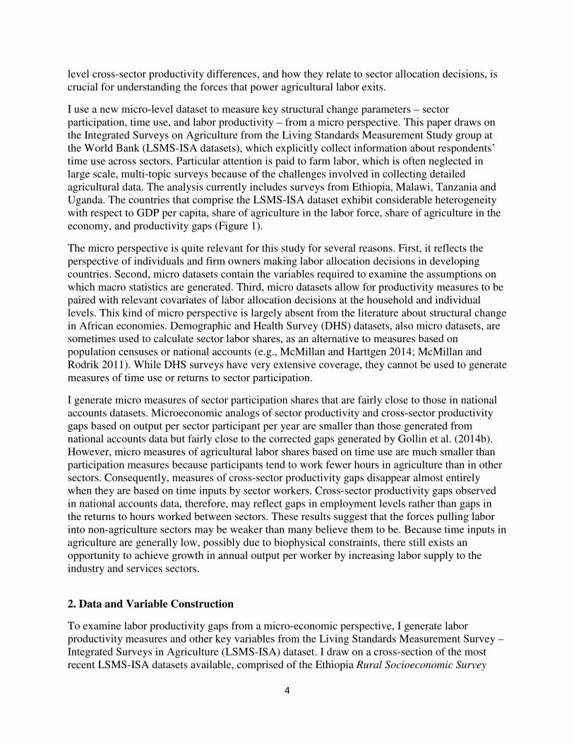
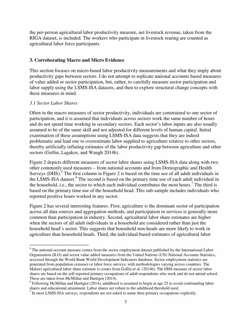
Figure 2 depicts different measures of sector labor shares using LSMS-ISA data along with two other commonly used measures – from national accounts and from Demographic and Health Surveys (DHS).5 The first column in Figure 2 is based on the time use of all adult individuals in the LSMS-ISA dataset.6 The second is based on the primary time use of each adult individual in the household, i.e., the sector to which each individual contributes the most hours.7 The third is based on the primary time use of the household head. This sub-sample includes individuals who reported positive hours worked in any sector.

Figure 2 has several interesting features. First, agriculture is the dominant sector of participation across all data sources and aggregation methods, and participation in services is generally more common than participation in industry. Second, agricultural labor share estimates are higher when the sectors of all adult individuals in a household are considered rather than just the household head’s sector. This suggests that household non-heads are more likely to work in agriculture than household heads. Third, the individual-based estimates of agricultural labor

5 The national account measure comes from the sector employment dataset published by the International Labor

Organization (ILO) and sector value added measures from the United Nations (UN) National Accounts Statistics, accessed through the World Bank World Development Indicators database. Sector employment statistics are generated from population censuses or labor force surveys, with methodologies varying across countries. The Malawi agricultural labor share estimate is comes from Gollin et al. (2014b). The DHS measure of sector labor shares are based on the self-reported primary occupations of adult respondents who work and do not attend school. These are taken from McMillan and Harttgen (2014). 6 Following McMillan and Harttgen (2014), adulthood is assumed to begin at age 25 to avoid confounding labor

shares and educational attainment. Labor shares are robust to the adulthood threshold used. 7 In most LSMS-ISA surveys, respondents are not asked to name their primary occupations explicitly.

8

shares are generally close to and slightly larger than the national-accounts measures in all countries except Malawi, where they are slightly smaller. Fourth, the DHS-based measures of agricultural participation shares are quite a bit lower than the LSMS-based individual participation shares except in Uganda, where they are almost identical. This implies that DHS-based labor share estimates might under-estimate agricultural labor shares and therefore overestimate labor productivity in agriculture relative to other sectors. Since individuals self-identify their primary sector in DHS surveys, it is possible that respondents involved in multiple sectors are more likely to identify the non-agriculture occupation even though it accounts for a lower share of labor supplied.

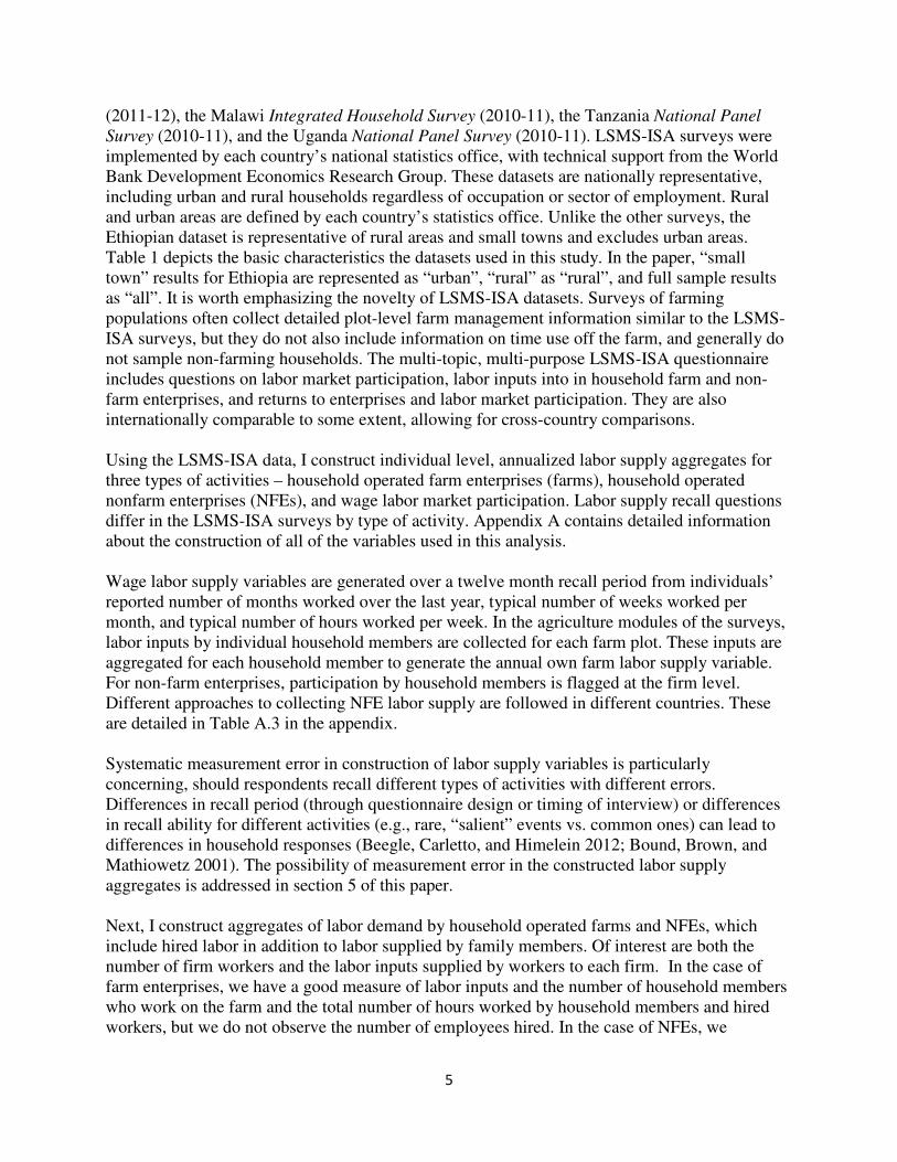
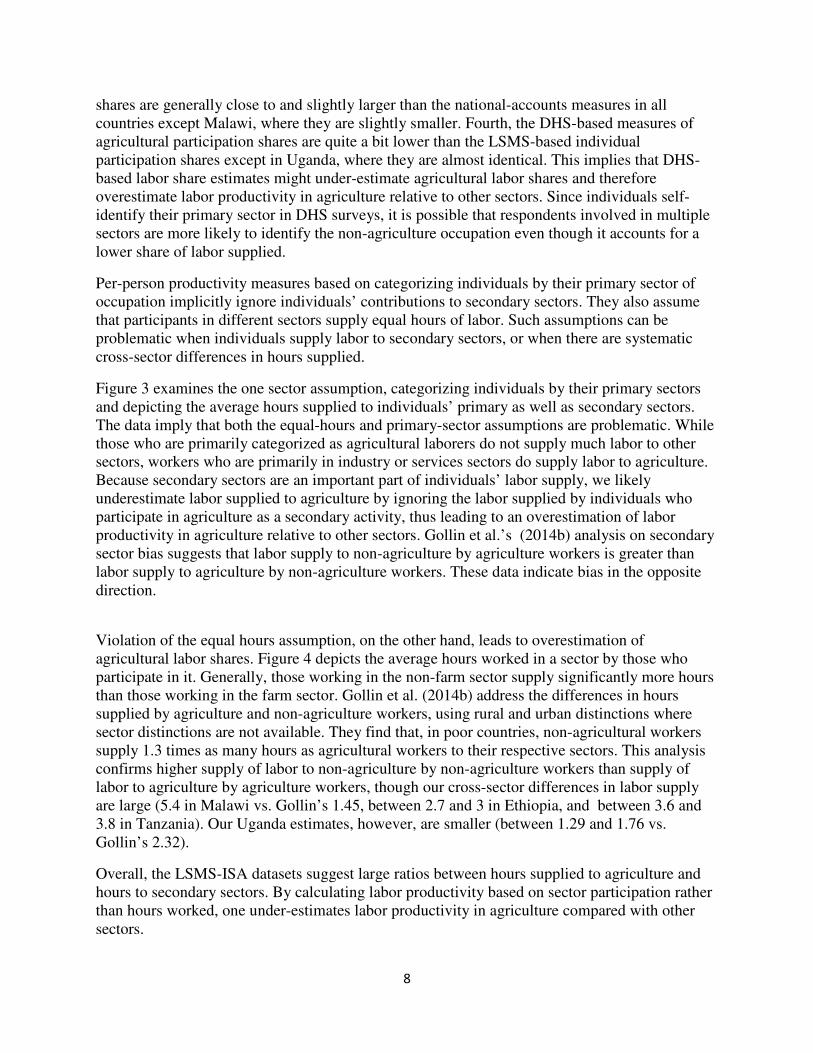
Per-person productivity measures based on categorizing individuals by their primary sector of occupation implicitly ignore individuals’ contributions to secondary sectors. They also assume that participants in different sectors supply equal hours of labor. Such assumptions can be problematic when individuals supply labor to secondary sectors, or when there are systematic cross-sector differences in hours supplied.

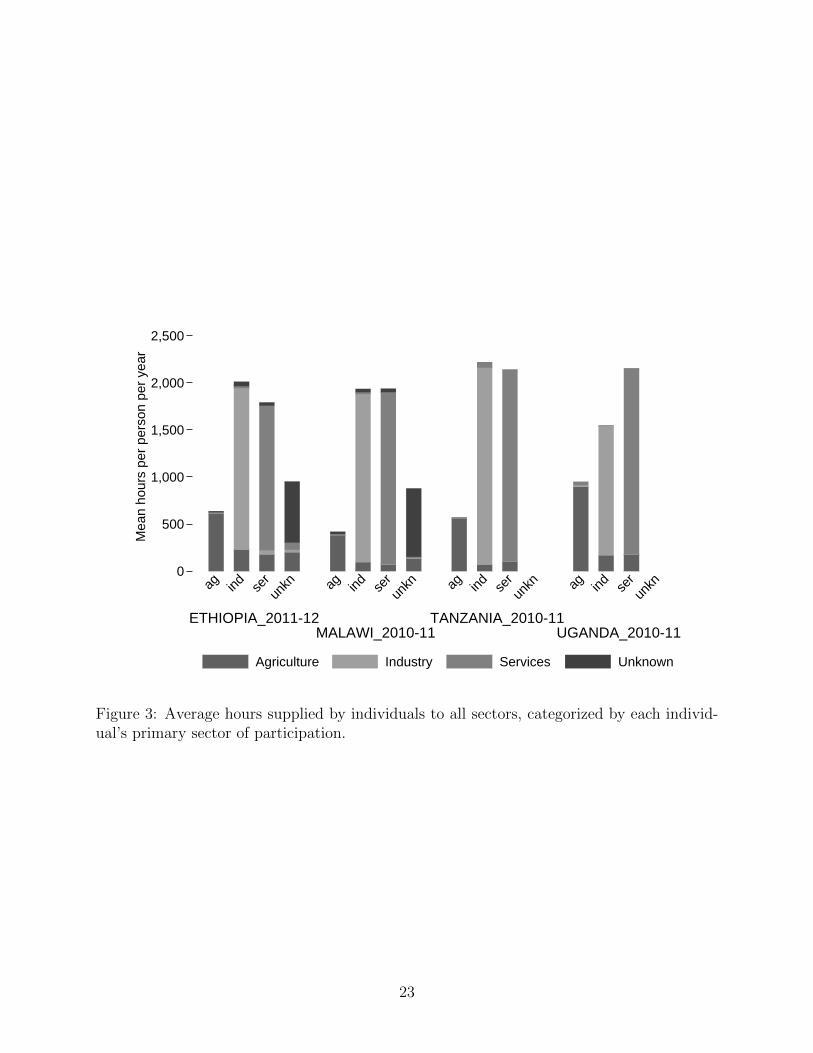
Figure 3 examines the one sector assumption, categorizing individuals by their primary sectors and depicting the average hours supplied to individuals’ primary as well as secondary sectors. The data imply that both the equal-hours and primary-sector assumptions are problematic. While those who are primarily categorized as agricultural laborers do not supply much labor to other sectors, workers who are primarily in industry or services sectors do supply labor to agriculture. Because secondary sectors are an important part of individuals’ labor supply, we likely underestimate labor supplied to agriculture by ignoring the labor supplied by individuals who participate in agriculture as a secondary activity, thus leading to an overestimation of labor productivity in agriculture relative to other sectors. Gollin et al.’s (2014b) analysis on secondary sector bias suggests that labor supply to non-agriculture by agriculture workers is greater than labor supply to agriculture by non-agriculture workers. These data indicate bias in the opposite direction.

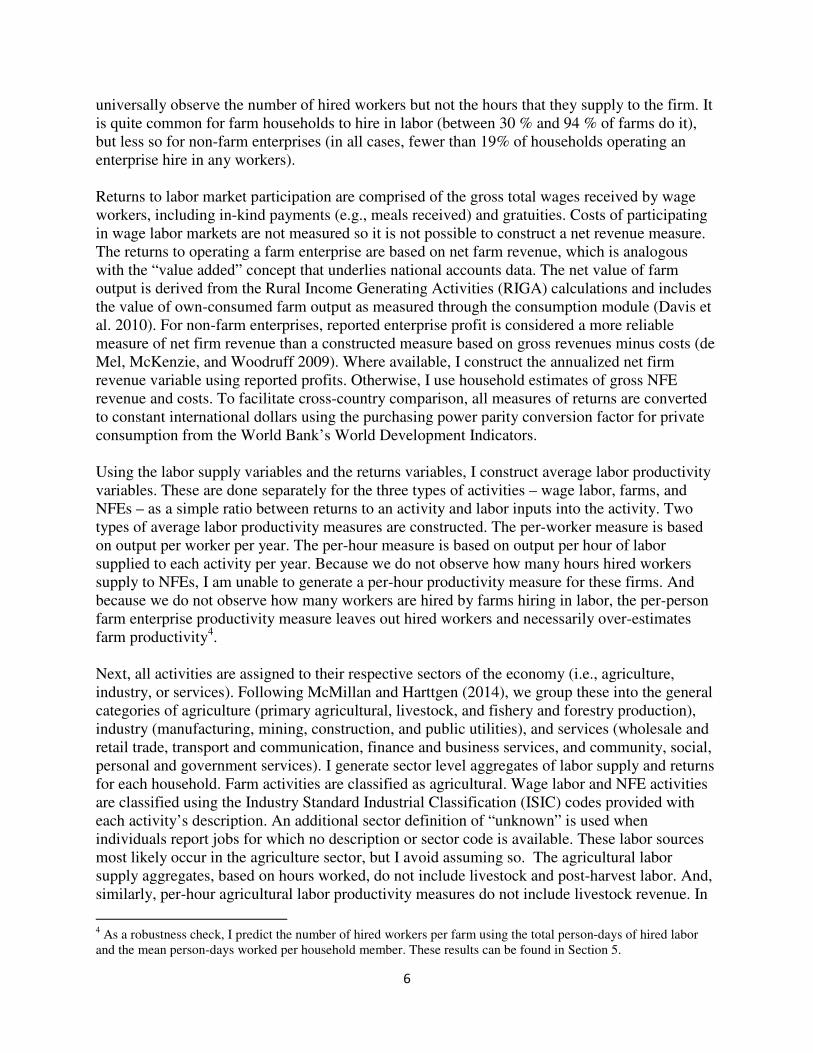
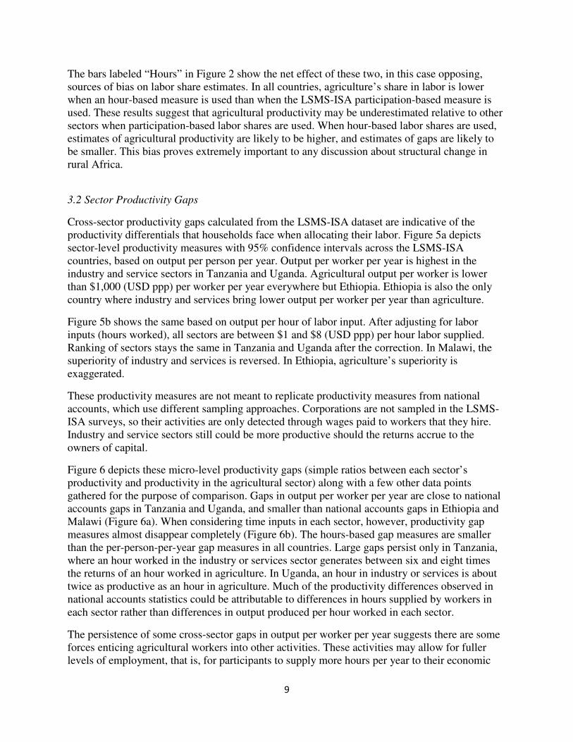
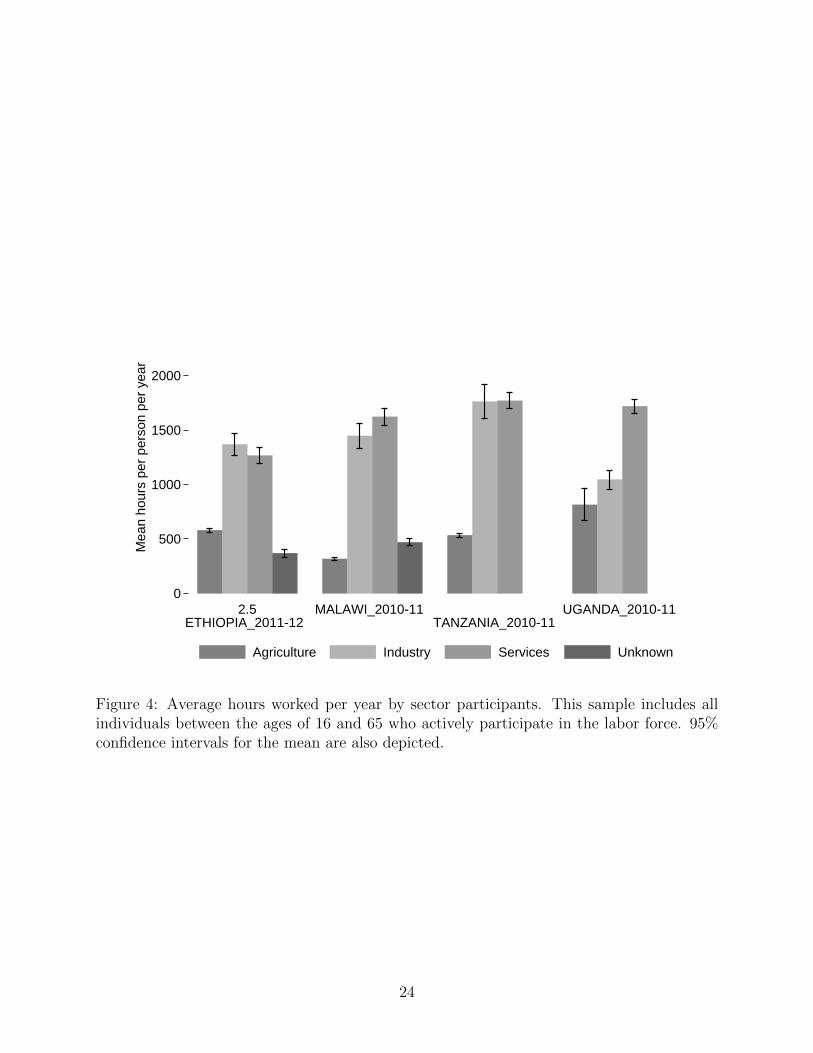
Violation of the equal hours assumption, on the other hand, leads to overestimation of agricultural labor shares. Figure 4 depicts the average hours worked in a sector by those who participate in it. Generally, those working in the non-farm sector supply significantly more hours than those working in the farm sector. Gollin et al. (2014b) address the differences in hours supplied by agriculture and non-agriculture workers, using rural and urban distinctions where sector distinctions are not available. They find that, in poor countries, non-agricultural workers supply 1.3 times as many hours as agricultural workers to their respective sectors. This analysis confirms higher supply of labor to non-agriculture by non-agriculture workers than supply of labor to agriculture by agriculture workers, though our cross-sector differences in labor supply are large (5.4 in Malawi vs. Gollin’s 1.45, between 2.7 and 3 in Ethiopia, and between 3.6 and 3.8 in Tanzania). Our Uganda estimates, however, are smaller (between 1.29 and 1.76 vs. Gollin’s 2.32).

Overall, the LSMS-ISA datasets suggest large ratios between hours supplied to agriculture and hours to secondary sectors. By calculating labor productivity based on sector participation rather than hours worked, one under-estimates labor productivity in agriculture compared with other sectors.

9

The bars labeled “Hours” in Figure 2 show the net effect of these two, in this case opposing, sources of bias on labor share estimates. In all countries, agriculture’s share in labor is lower when an hour-based measure is used than when the LSMS-ISA participation-based measure is used. These results suggest that agricultural productivity may be underestimated relative to other sectors when participation-based labor shares are used. When hour-based labor shares are used, estimates of agricultural productivity are likely to be higher, and estimates of gaps are likely to be smaller. This bias proves extremely important to any discussion about structural change in rural Africa.

3.2 Sector Productivity Gaps

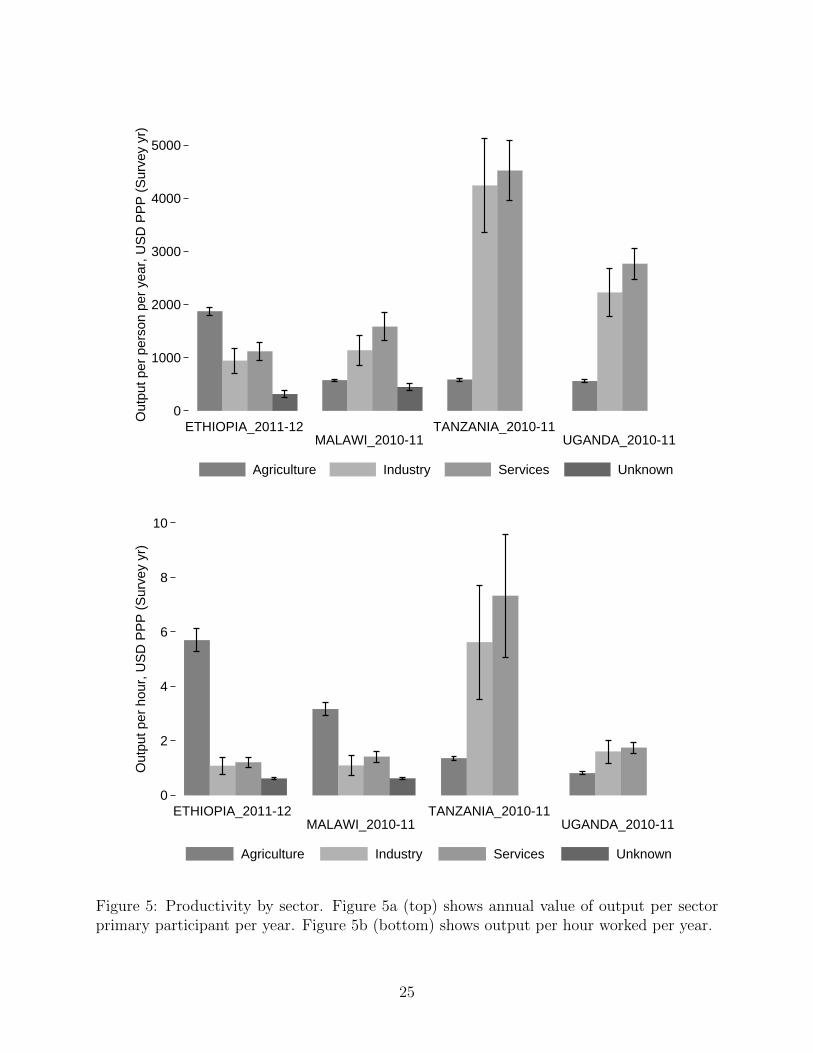
Cross-sector productivity gaps calculated from the LSMS-ISA dataset are indicative of the productivity differentials that households face when allocating their labor. Figure 5a depicts sector-level productivity measures with 95% confidence intervals across the LSMS-ISA countries, based on output per person per year. Output per worker per year is highest in the industry and service sectors in Tanzania and Uganda. Agricultural output per worker is lower than $1,000 (USD ppp) per worker per year everywhere but Ethiopia. Ethiopia is also the only country where industry and services bring lower output per worker per year than agriculture.

Figure 5b shows the same based on output per hour of labor input. After adjusting for labor inputs (hours worked), all sectors are between $1 and $8 (USD ppp) per hour labor supplied. Ranking of sectors stays the same in Tanzania and Uganda after the correction. In Malawi, the superiority of industry and services is reversed. In Ethiopia, agriculture’s superiority is exaggerated.

These productivity measures are not meant to replicate productivity measures from national accounts, which use different sampling approaches. Corporations are not sampled in the LSMS-ISA surveys, so their activities are only detected through wages paid to workers that they hire. Industry and service sectors still could be more productive should the returns accrue to the owners of capital.

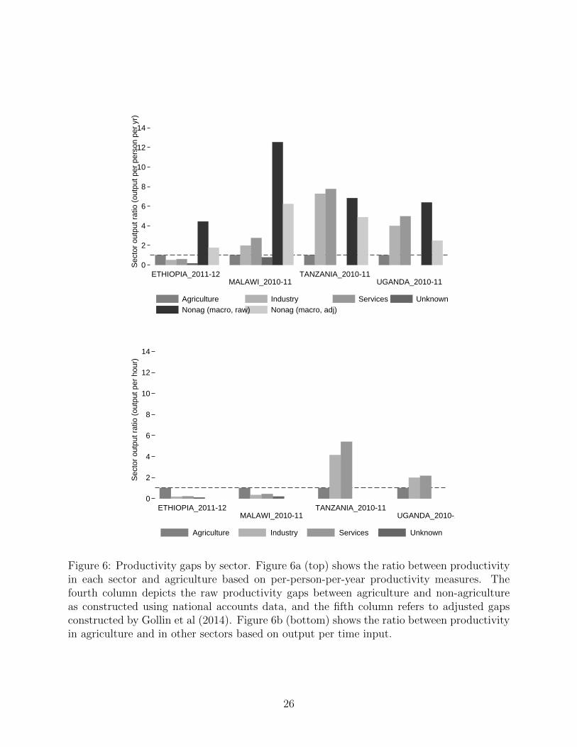
Figure 6 depicts these micro-level productivity gaps (simple ratios between each sector’s productivity and productivity in the agricultural sector) along with a few other data points gathered for the purpose of comparison. Gaps in output per worker per year are close to national accounts gaps in Tanzania and Uganda, and smaller than national accounts gaps in Ethiopia and Malawi (Figure 6a). When considering time inputs in each sector, however, productivity gap measures almost disappear completely (Figure 6b). The hours-based gap measures are smaller than the per-person-per-year gap measures in all countries. Large gaps persist only in Tanzania, where an hour worked in the industry or services sector generates between six and eight times the returns of an hour worked in agriculture. In Uganda, an hour in industry or services is about twice as productive as an hour in agriculture. Much of the productivity differences observed in national accounts statistics could be attributable to differences in hours supplied by workers in each sector rather than differences in output produced per hour worked in each sector.

The persistence of some cross-sector gaps in output per worker per year suggests there are some forces enticing agricultural workers into other activities. These activities may allow for fuller levels of employment, that is, for participants to supply more hours per year to their economic

10

activities. This analysis cannot disentangle whether differences in hours worked across sectors are determined by sector level labor supply or demand characteristics. It could be that agricultural labor demand is not well smoothed throughout the year. Because of biophysical and agricultural constraints, it might not be possible for individuals to increase their agricultural sector returns by supplying more hours to their farms. Presumably, because employment is so limited across Sub-Saharan Africa, low demand for labor by agriculture is a key constraint. Understanding what limits supply and/or demand of labor in the agricultural sector is an important topic that is left for future research.

4. Exploring the Non-Farm Economy

This section contains a close examination of the non-farm activities in which households are involved, with a view towards understanding their implications for structural change patterns and prospects. 4.1 Household and worker characteristics

It is important to explore any systematic differences in characteristics of sector participants, so that they can be taken into account when using national accounts data on sector labor shares. Indeed, the macro-economic literature is concerned with systematic differences in human capital across sectors and the implications for bias in productivity measures (Vollrath 2014). Table 2 includes basic summary statistics according to individuals’ primary sectors of participation.

There are no major differences in the average age of each sector’s work force in any country. In Malawi, Tanzania, and Uganda, the agricultural work forces are slightly more female, while the industry and services work forces are strongly male. On the other hand, in Ethiopia, the agricultural work force is slightly more male than female, while the industry and services work forces are slightly more female. Individuals who do not supply hours to any sector are younger and more female, on average, than individuals who do. The average years of education completed tend to be highest in the services sector and lowest in the agricultural sector. The educational differences point to possible systematic skill differences across sector work forces. However, individuals who do not participate in any sector, on average, have education levels similar to those of industry workers, and higher than agricultural workers.

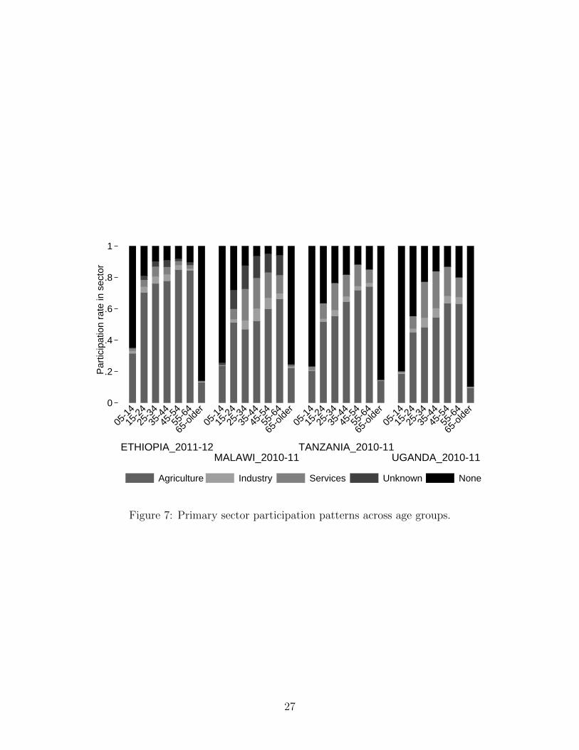
Figure 7 depicts the changing primary sector of workers across all major age cohorts. Youth (ages 15-24) generally have lower participation in economic activities than do young adults (ages 25-34). Economically active youth have similar labor shares to economically active young adults, though they have higher rates of participation in agriculture and lower rates in industry and services. Despite these differences, labor shares are robust to the specification of the “adulthood” threshold at age 25 rather than age 15.8

There is always concern that differences in productivity observed between different activities reflect differences in the households participating in the activities rather than inherent differences in the economic productivity of the activities themselves. Productivity-determining characteristics may or may not be observed in survey datasets. I explore the possible contribution

8 Results can be shared upon request.

11

of differences in household characteristics to productivity gaps by generating productivity measures for each sector-activity combination at the household level. This includes household farms, household-owned NFEs, and household wage labor in all sectors. Wages are not, of course, a productivity measure, especially in the presence of market frictions, of which the evidence is strongly suggestive (Dillon and Barrett 2014). They do offer a lower bound on the marginal revenue product of hired labor, and they also provide a benchmark against which individuals in an economy can evaluate self vs. own employment.

Figure 8 depicts these sector-activity productivity gaps based on mean returns to each sector-activity compared with mean returns to farming. The labor inputs of hired workers are included alongside household workers whenever possible. As previously mentioned, the per-person farm productivity estimates do not include hired labor and therefore necessarily over-estimate output per farm worker. Firm level per-hour productivity estimates are not included for NFEs because good time input measures are not available for these firms.

The patterns here are similar to those observed with the sector level analysis. First, mean returns per participant per year are higher outside of farming in many cases – for wage laborers in Malawi, and for enterprise operators and industry and sector wage workers in Tanzania and Uganda. NFEs and wage laborers often each bring lower returns per participant per year than do household farm workers. The unconditional (cross-household) and conditional (intra-household) productivity gaps are similar in magnitude to the sector productivity gaps. These gaps also shrink considerably, except in Tanzania, when labor inputs are considered.

Using the sector-activity productivity measures, I next calculate conditional productivity gaps, or within-household gaps between farming and other activities for farming households that also participate in an additional activity. Figure 9 depicts these conditional gaps – measured as the median across households of cross-sector gaps observed within households that participate in multiple activities. The conditional productivity gap for agricultural wages, for example, is based on a comparison between farm returns and agricultural wages only for households that participate in farming and agricultural wage labor.

In comparison with the unconditional productivity gaps, the conditional gaps are informative. If

households are equating returns across sectors where we see them in multiple sectors simultaneously (i.e. the conditional productivity gap measures), then the differences in returns observed in the unconditional productivity gap measures reflect selection effects related to a household’s ability to participate in an activity. This is consistent with the idea of human capital heterogeneity across sectors. The observed small magnitude of intra-household gaps also suggests that structural barriers to improved household productivity that span across sectors may constrain households’ opportunities to raise their productivity levels.

4.2 Jobs and Non-Farm Enterprises

Table 3 summarizes individuals’ participation in own account and wage labor activities by sector, describing participation rates and basic characteristics of participants for both rural (Table 3a) and urban (Table 3b) populations. Additional analysis of the NFEs that occur in the LSMS-ISA datasets can be found in Nagler and Naudé (2014).

12

Participation in own-account activities is certainly most popular across the board, with 74-89% of rural adults participating in farming. Agricultural wage labor participation is less common, with fewer than 10% of rural adults participating in Ethiopia, Tanzania and Malawi, and just 15% in Uganda. In all countries, the average agricultural wage laborer is much more likely to be male than the average farm worker. Agricultural wage workers have more education, on average, than farm workers in Ethiopia and Malawi, and less in Tanzania and Uganda. Because Ethiopia and Malawi surveys collect casual wage labor that cannot be matched to a sector, it is likely that low skill agricultural laborers are showing up in the “unknown” sector. Within the industry sector, rural individuals are more likely to participate as own account workers everywhere but Uganda. However, in Malawi, 30% of rural individuals participate in own-account industry sector activities, most of which are related to manufacturing. The industrial sector comprises less than 10% of the labor force everywhere but Malawi, where it surpasses 30%. Industry wage laborers are very strongly male, while industry own-account workers are mostly female. Urban participation in industry sector activities is slightly higher than is rural participation everywhere except Malawi. Participation in the services sector by urban and rural workers is much higher than participation in the industry sector in all countries. Participation as own account workers is higher than participation as wage laborers among all urban and rural workers except for in Ethiopian small town areas. Wage labor participants in the services sector are very strongly male and have higher education levels than own account service sector participants. Both wage and services sector participants supply similar numbers of hours per year except in Tanzania, where own account service sector workers supply far fewer hours than do wage laborers. Table 4 breaks down wage and NFE activities by a more granular list of sectors. For the enterprise columns, the total number of households in the dataset is provided, along with the number of households that operate at least one enterprise, and the total number of firms present in the dataset (this final number is larger because some households operate more than one firm). Then the firms are categorized by ten sub-sectors of the economy. For the jobs columns, the total number of individuals of working age is provided, along with the total number who participate in wage labor, and the total number of jobs reported in the dataset. Again, because some individuals have more than one source of wage-earning income, this number is larger than the number of wage market participants. The industry sector is divided into mining, manufacturing, electricity and utilities, and construction. The services sector is comprised of commerce, transport and communication, general services, and finance. A summary of activities is provided separately for rural and urban areas (Tables 4a and 4b, respectively). I use respondents’ free descriptions of their NFEs and jobs, along with the specific industry codes provided by enumerators, to examine carefully the kinds of non-farm activities in which respondents are involved. We do not observe the level of formality associated with household firms and wage-earning jobs because there is not enough comparability across survey questionnaires to describe formality of employment arrangements and/or firm registration.

13

Agricultural wage labor is the largest category of employment in rural Tanzania and Uganda. In Ethiopia and Malawi, the highest category is “unknown” sector wage employment, which is casual wage labor for which no sector codes or job descriptions were collected. Most likely, this labor is supplied to the agriculture sector9. Based on the descriptions provided, most agricultural jobs involve casual labor on farms for food or cash crop production, or they involve livestock tending, hunting, fishing, and collection of forestry products, such as fuel wood. Agricultural sector NFEs, of which there are few, also tend to be businesses associated with the production of livestock, fishery, or forestry products. Within the industry sector, mining does not play an important role in rural or urban areas of any of the datasets we analyze. Manufacturing accounts for between 14% and 38% of NFEs, with the smallest share in Tanzania and the largest in Malawi. However, only 2-6% of jobs occur in manufacturing. Manufacturing NFEs focus heavily on elementary activities such as brewing of alcoholic beverages, charcoal production, milling grains, butchering and other agricultural processing, baking and other value addition activities, and the production of textiles as well as weaving and other handicrafts. Manufacturing jobs are similar, with a focus on agri-processing for food, timber, and textiles, as well as the manufacturing of bricks and other construction materials. Utilities provision is not an important source of employment anywhere, nor is it a key focus of household firms, except for in Ethiopia. Construction accounts for between 2% and 7% of rural jobs and between 5% and 10% of urban jobs but fewer than 2% of NFEs. Construction firms tend to focus on brick-laying and building construction, while construction jobs include working as a laborer in the construction of a road or building and contracting. Individuals and households who participate in the industry sector are involved mainly in manufacturing activities that have strong links with primary agricultural production. Industry sector participants contribute to manufacturing raw agricultural materials into typically non-tradable goods meant for local consumption. These patterns suggest strong links between rural industry-sector activities and agricultural activities. In rural areas, the manufacturing industry stands to gain from productivity growth in agriculture, and rural manufacturing workers are poised to benefit from demand spurred by rising agricultural incomes in rural areas. Because the manufacturing activities reported in these surveys are so closely linked with agriculture, one would not expect to see expansion of rural industry sector activities independently, without any agricultural growth. These classic Mellor-Johnston linkages are quite prominently featured in rural households’ economic activities. Commerce is the dominant focus of NFEs in the services sector, while jobs tend to involve general services provision. Commerce comprises of between 30% and 66% of both rural and urban firms. These are involved in activities such as the wholesale and retail trade of fruits and vegetables, other food items, charcoal, second hand goods, and other household goods. Commerce accounts for up to 20% of jobs in urban areas of Tanzania, but the share is more often closer to 5%-10% in urban areas, and lower in rural areas. Commerce wage earners are most commonly sales clerks and store attendants. The transport sub-sector accounts for about 8% of Ethiopian firms, and a much smaller share of firms and jobs elsewhere. Transport activities tend to focus on transportation services provided by bicycle, taxi, bus, or vehicle. Finance and real

9 This impression is based on my own experience shadowing LSMS-ISA survey teams in Ethiopia during the 2012-13 round of surveys, and on discussions with survey teams from both countries.

14

estate are almost nonexistent in rural areas and account for 1%-3% of urban jobs, which are most commonly administrative in nature. Finally, the general services category is the most important, accounting for 40%-50% of urban jobs across all countries, and 15%-30% of rural jobs in Ethiopia and Malawi and 25% in Tanzania and Uganda. These wage workers include teachers, health, social and religious workers, public administrators, technicians, domestic service providers, as well as restaurant, hotel, and tourism employees. General services account for a smaller share of firms than of employment. The firms typically involve restaurants and caterers, bars, hotels, professional service providers, and repair shops. Buying and selling agricultural products comprises a large share of commerce NFE activity and wage employment. As with the industry sector, the services sector activities in which rural households participate are non-tradable in nature, and very focused on local consumers. Because these service-sector activities serve local consumers whose incomes are dominated by agriculture-sector activities, the Mellor-Johnston linkages are again quite prominent. One would expect agricultural productivity growth to spur demand for increased local service sector labor. Given the nature of service sector activities, one would not expect to see strong growth in the services sector absent agricultural growth.

5. Robustness of productivity gap measurement

Sector productivity gap estimates are sensitive to prospective measurement error of firm revenue and wage earnings. Consumption can be thought of as household profits after participation costs (for wage labor) and production costs (for firms), assuming no savings or dissavings. Because households who face stochastic income generally smooth their consumption from year to year, consumption can be a good measure of permanent income (Bhalla 1978). It is a central focus of LSMS-ISA surveys to generate consumption aggregates, so this variable plays to the strengths of the data. Consumption aggregates are generated by each country’s statistics office and released with the datasets. They include cash expenditures as well as the imputed value of items that are produced and consumed by the household, such as agricultural goods. The consumption gap estimates are a ratio in per capita consumption between households participating primarily in agriculture and those participating primarily in industry and services, respectively (Figure 10).

These gaps are fairly similar across countries, and are considerably smaller than productivity gaps, though they follow similar rankings. Households primarily in the industry sector consume 1.2-3 times more per capita per year than agricultural households. Households primarily in the services sector consume 1.5-4 times more per capita per year than agricultural households. The consumption gaps are quite similar in magnitude to the per-person-per-year productivity gaps. They are slightly larger in Ethiopia and Malawi, and smaller in Tanzania and Uganda. As with productivity gaps, consumption gaps also disappear almost entirely when they are expressed per hour of labor supplied by each household. This suggests that differences in consumption across sectors (as with differences in returns to sector participation) can be explained in large part by differences in hours worked across sectors.

Because labor supply variables for different activities are constructed from different types of survey questions, there is concern that differences in labor supply across activities could arise from different survey recall approaches rather than actual labor supply differences. To address this concern, I construct an alternate set of labor supply variables using only 7-day recall

15

questions. These lend themselves better to cross-sector comparison because a common recall period is used to elicit time spent working for a household farm, a NFE, and as a wage laborer. At least for any one week, the ratio should reflect the ratio of labor supply, minimizing questionnaire bias. It remains possible that individuals recall different types of activities differently within the 7-day recall window. It is also important to note that the 7-day recall question about labor supplied to a household farm explicitly includes livestock labor, whereas the season-wide plot-based labor recall variable is restricted to crop production and excludes livestock related labor. We would expect a 7-day recall of crop activities, which would be comparable to the season-wide variable to be smaller than a 7-day recall of both crop and livestock activities10.

The same-recall-method mean labor supply aggregates are depicted in Figure 11a, in the left column. Indeed, these labor supply variables skew more heavily towards agriculture than do labor

supply variables based on different recall methods. The difference is mostly due to differences in the absolute labor supply measure for agriculture, though the 7-day aggregate was multiplied by 52 weeks per year to facilitate comparison with the 12-month aggregates. It is not entirely clear whether surveys are more or less likely to take place during the agricultural off-season. The NFE and wage labor supply estimates are quite similar across recall periods. This does raise some concerns that, when farm labor inputs are recalled over the season by plot task for each household member, farm inputs are underestimated. Further research is required to better understand the implications of different recall and reference periods in agricultural labor measurement.

For each type of activity, I include a non-parametric regression of a labor supply variable based on 7-day recall and a labor supply variable based on 12-month recall (Figure 11b).11 In all countries, for the majority of individuals, a higher farm labor supply estimate is reached based on the 7-day recall than the 12-month recall. In Malawi and Uganda, those who have the highest seasonal estimates of farm labor supply (more than 600 hours per year) do not report correspondingly high agricultural labor supply over 7-day recall.

Regarding NFE and wage labor, the results are consistent with a situation in which seasonality plays a role. There is a tendency for those who report lower total labor supply based on 12-month recall to report higher labor supply over a 7-day period. There is also a tendency for those who report high labor supply based on 12-month recall to report lower supply based on 7-day recall. This analysis further highlights the need to separately measure livestock inputs, to better understand the seasonality of farm labor inputs, and to better understanding farm labor recall. In a world with seasonality but without questionnaire bias, the mean labor supply aggregates would be the same for 7-day and 12-month recall if the survey took place throughout the year. The 7-day aggregates would be higher if more surveys took place during busier periods and lower if more surveys took place during less busy periods. More respondents’ labor supply aggregates based on 7-day recall are higher than those based on 12-month recall for all activities except wage labor, indicating either that the surveys take place during busier periods or that the 7-day

10

Seasonality is also a concern. In most of the surveys, the visits were timed to reduce the effect of seasonality, so that sample-wide averages are also cross-season averages. This is not the case in Ethiopia, where the household interviews nationwide were conducted within a short window. 11

The regressions are visually weighted, with the predicted values stronger where there is higher density of data, and more feint at the tails of the distribution, following Hsiang (2012).

16

measures are upwardly biased. Because the number of hired farm workers is not observed, the farm level count of farm workers is under-estimated, as it only includes household members who work on the farm. Underestimation of the number of farm workers leads to upward bias in estimates of annual farm output per worker and downward bias in the productivity gaps between household farms and other activities (i.e., wage labor and NFEs in various sectors) that are depicted in Figure 8a and Figure 9a. Hiring in of some farm labor, though, is a common practice. I use the average hours worked on the farm per household farm worker to convert the hours worked by hired farm workers into a predicted number of hired farm workers. I then predict a new estimate of farm output per farm worker, and calculate new unconditional and conditional productivity gaps between household farms, NFEs and wage labor. These can be found in the Figure 12. These alternative measures of farm labor productivity gaps are slightly larger, but the effect is small, and the overall story remains the same.

6. Conclusion

Micro level cross-sector labor productivity gaps are smaller than those generated using national accounts data and vanish almost completely when computed on a per-hour basis. The ratios of consumption levels per capita between households that primarily participate in agriculture vs. other sectors are also small, confirming small cross-sector gaps in returns to sector participation. Inter-sectoral differences in annual earnings per worker arise from differences in employment volume (hours per worker of labor supplied) rather than wages or productivity per hour of labor supplied. The tendency is for individuals participating in agriculture to supply fewer hours to agriculture, on average, than individuals participating in other sectors. The findings underscore agriculture’s importance to structural transformation in Sub-Saharan Africa. Agriculture, and specifically the operation of household farms, remains a dominant economic activity in rural areas of Sub-Saharan Africa. And, furthermore, much of the labor supplied to industry and services sectors involves the processing and trading of agricultural and other primary goods for consumers whose incomes are dominated by agriculture-sector activities. Furthermore, the non-farm activities in which rural households are involved, across countries, are incredibly closely linked with agriculture. These strong links highlight additional benefits to achieving agricultural productivity growth, which can increase the supply of raw materials for manufacturing and increase the demand for non-tradable goods and services. These linkages are also sobering as, apart from agriculture, no engine for rural economic growth is apparent. Generally, the micro evidence seems consistent with the idea that there is scope for releasing labor from agriculture should it be demanded by other sectors. Households expect industry and service sector wage workers to earn higher returns per year than farm workers. Non-farm enterprises can bring higher annual returns to participants than farm enterprises in some countries, and much lower in others. This remains true when comparing within-household returns only for households participating in multiple activities, though, in this case, off-farm returns look much closer to farm returns.

17

Small per-worker-per-year micro productivity gaps suggest that workers, who are the owners of labor, may not stand to reap the large benefits of labor exiting agriculture that are expected in the economy as a whole (should national accounts data indeed reflect true economy-wide productivity gaps). Small per-worker-per-year micro gaps also suggest that agriculture-sector workers do not feel as strong a “pull” from industry and services as one might expect based on national accounts data. However, the evidence also suggests that individuals and households may face barriers to participation in non-agriculture activities. Workers who primarily participate in the industry and service sectors are able to participate in agriculture, while the reverse is not true of workers who are primarily agricultural. Service sector participants, in particular, tend to have higher education levels than workers in other sectors. Some households may face structural barriers to labor productivity growth that span across multiple sectors. The small size of conditional gaps (within-household gaps faced by participants in multiple sectors) relative to unconditional gaps (pooled, cross-sector gaps) suggests that selection effects into non-agriculture activities contribute to cross-sector productivity differentials. Households who are unable to diversify might face even smaller productivity gains outside of agriculture than those who are, further eroding the benefits of structural reallocation of labor.

Nonexistent per-hour micro gaps suggest that differences in the annual output of agricultural workers vs. industry and service sector workers, whether observed in micro or macro data, might be largely explained by differences in hours worked in agriculture vs. in industry and services. Small per-hour gaps do not undermine agriculture’s role in structural transformation. Despite low per-hour gaps in agriculture, it appears that workers have an excess of labor that could be absorbed productively in other sectors. This requires growth in demand for labor outside of agriculture. Why these employment gaps exist is not well understood. They raise the question of what limits the supply of hours in the agricultural sector and what role technology, infrastructure and policies might play in closing the cross-sector employment gaps. Is it the time-sensitivity of agricultural labor demand, or, more generally, seasonality? If so, could demand be smoothed with water control technologies and infrastructure? Is it barriers to participate in non-farm self or wage employment? Is it financial constraints that prevent farmers from procuring non labor complements? The results suggest that the upside to “saving” agricultural labor may not be very big, placing the onus on numerator (i.e. output value) driven productivity growth.

Overall, the analysis emphasizes agriculture’s key role in Sub-Saharan African economies, while also raising questions about agricultural employment gaps, their determinants, and how they shape the opportunity to achieve economy-wide labor productivity growth. A between-sector gradient in annual output per worker remains to be exploited. Improving annual output per worker within agriculture, the highest participation sector by far, requires a better understanding of labor demand by smallholder farmers.

18

References

Barrett, Christopher B., T Reardon, and P Webb. 2001. “Nonfarm Income Diversification and Household Livelihood Strategies in Rural Africa: Concepts, Dynamics, and Policy Implications.” Food Policy 26 (4) (August): 315–331.

Beegle, Kathleen, Calogero Carletto, and Kristen Himelein. 2012. “Reliability of Recall in Agricultural Data.” Journal of Development Economics 98 (1) (May): 34–41.

Beegle, Kathleen, Joachim De Weerdt, and Stefan Dercon. 2011. “Migration and Economic Mobility in Tanzania: Evidence from a Tracking Survey.” Review of Economics and

Statistics 93 (August): 1010–1033.

Bhalla, Surjit S. 1978. “The Role of Sources of Income and Investment Opportunities in Rural Savings.” Journal of Development Economics 5 (3) (September): 259–281.

Block, Steven A. 2013. “The Post-Independence Decline and Rise of Crop Productivity in Sub-Saharan Africa: Measurement and Explanations.” Oxford Economic Papers (March 23).

Bound, John, Charles Brown, and Nancy Mathiowetz. 2001. “Measurement Error in Survey Data.” In Handbook of Econometrics, edited by James J Heckman and B T Leamer, Volume 5:3705–3843. Elsevier.

Christiaensen, Luc, Lionel Demery, and Jesper Kuhl. 2011. “The (evolving) Role of Agriculture in Poverty reduction—An Empirical Perspective.” Journal of Development Economics 96 (2): 239–254.

Collier, Paul, and Stefan Dercon. 2014. “African Agriculture in 50 Years: Smallholders in a Rapidly Changing World?” World Development 63 (November 2014): 92–101.

Davis, Benjamin, Stefania Di Giuseppe, and Alberto Zezza. 2014. “Income Diversification Patterns in Rural Sub-Saharan Africa Reassessing the Evidence.” World Bank Policy

Research Working Paper No. 7108.

Davis, Benjamin, Paul Winters, Gero Carletto, Katia Covarrubias, Esteban J. Quiñones, Alberto Zezza, Kostas Stamoulis, Carlo Azzarri, and Stefania DiGiuseppe. 2010. “A Cross-Country Comparison of Rural Income Generating Activities.” World Development 38: 48–63.

De Janvry, Alain, and Elisabeth Sadoulet. 2009. “Agricultural Growth and Poverty Reduction : Additional Evidence.” World Bank Reserach Observer 25 (1): 1–20.

De Mel, Suresh, David J. McKenzie, and Christopher Woodruff. 2009. “Measuring Microenterprise Profits: Must We Ask How the Sausage Is Made?” Journal of Development

Economics 88 (1) (January): 19–31.

19

Dercon, Stefan. 2009. “Rural Poverty: Old Challenges in New Contexts.” World Bank Research

Observer 24 (1): 1–28.

Dillon, Brian, and Christopher B Barrett. 2014. “Agricultural Factor Markets in Sub-Saharan Africa An Updated View with Formal Tests for Market Failure.” World Bank Policy

Research Working Paper No. 7117.

Foster, AD, and MR Rosenzweig. 2003. “Agricultural Development, Industrialization and Rural Inequality.” Mimeo. Harvard University.

Gollin, Douglas, David Lagakos, and Michael E Waugh. 2014a. “Agricultural Productivity Differences across Countries.” American Economic Review 104 (5): 165–170.

———. 2014b. “The Agricultural Productivity Gap.” Quarterly Journal of Economics 129 (2) (May 1): 939–993.

Haggblade, Steven, P. B. Hazell, and T. A. Reardon. 2007. “Structural Transformation of the Rural Nonfarm Economy.” In Transforming the Rural Nonfarm Economy: Opportunities

and Threats in the Developing World, edited by S. Haggblade, P. B. Hazell, and T. A. Reardon, Chapter 4. Baltimore, Md.: Johns Hopkins University Press.

Haggblade, Steven, Peter Hazell, and Thomas Reardon. 2010. “The Rural Non-Farm Economy: Prospects for Growth and Poverty Reduction.” World Development 38 (10): 1429–1441.

Headey, DD, and TS Jayne. 2014. “Adaptation to Land Constraints: Is Africa Different?” Food

Policy 48: 18–33.

Hsiang, Solomon M. 2012. “Visually-Weighted Regression.” Working Paper and Stata Code.

Lele, Uma, Manmohan Agarwal, and Sambuddha Goswami. 2013. “Lessons of the Global Structural Transformation Experience for the East African Community.” East African Community International Symposium and Exhibition on Agriculture. Kampala, Uganda.

McCaig, Brian, and Nina Pavcnik. 2013. “Moving out of Agriculture: Structural Change in Vietnam.” National Bureau of Economic Research Working Paper Series No. 19616.

McMillan, M, and Kenneth Harttgen. 2014. “What Is Driving the ‘African Growth Miracle’?.” National Bureau of Economic Research Working Paper Series No. 20077.

McMillan, M, and Derek Headey. 2014. “Introduction – Understanding Structural Transformation in Africa.” World Development 63: 1–10.

McMillan, M, and D Rodrik. 2011. “Globalization, Structural Change and Productivity Growth.” National Bureau of Economic Research Working Paper Series No. 17143.

20

McMillan, M, D Rodrik, and I Verduzco. 2014. “Globalization, Structural Change and Productivity Growth, with an Update on Africa.” World Development 63: 11–32.

Nagler, Paula, and Wim Naudé. 2014. “Non-Farm Enterprises in Rural Africa: New Empirical Evidence.” World Bank Policy Research Working Paper No. 7066.

Pardey, Philip G. 2014. “African Agricultural R&D and Productivity Growth in a Global Setting.” In Frontiers in Food Policy: Perspectives on Sub-Saharan Africa, edited by Walter P Falcon and Rosamond Naylor. Stanford Center on Food Security and the Environment.

Pingali, Prabhu L, Yves Bigot, and Hans P Binswanger. 1987. Agricultural Mechanization and

the Evolution of Farming Systems in Sub-Saharan Africa. Johns Hopkins University Press.

Rodrik, Dani. 2014. “An African Growth Miracle.” 2014. Richard H. Sabot Lecture, Center for Global Development. Washington, D.C.

Ruthenberg, Hans. 1971. Farming Systems in the Tropics. Oxford: Clarendon Press.

Timmer, C Peter. 1988. “The Agricultural Transformation.” In Handbook of Development

Economics, Vol ume1, edited by H B Chenery and T N Srinivasan, I:275–331. Amsterdam: Elsevier.

Vollrath, Dietrich. 2014. “The Efficiency of Human Capital Allocations in Developing Countries.” Journal of Development Economics 108 (0) (May): 106–118.

World Bank Group. 2014. “World Development Indicators.” http://databank.worldbank.org/data/views/variableselection/selectvariables.aspx?source=world-development-indicators.

Young, Alwyn. 2012. “The African Growth Miracle.” National Bureau of Economic Research

Working Paper Series No. 18490.

Labor productivity and employment gaps in Sub-Saharan AfricaAll figures and tables

0

20

40

60

80

100S

hare

6 7 8 9 10 11LN GDP Per Capita

Ag Employment Share:LSMS Sample Other Africa Non-AfricaAg Value Added Share:LSMS Sample Other Africa Non-Africa

0

5

10

15

Agr

icul

tura

l Pro

duct

ivity

Gap

s

6 7 8 9 10 11LN GDP Per Capita

LSMS Sample Other Africa Non-Africa

Figure 1: Figure 1a (top) shows a global cross-section of agricultural labor and employmentshares graphed against a log transformation of each country’s per capita GDP. Figure 1b(bottom) shows agricultural labor productivity gaps graphed against the log of GDP percapita (Source: Gollin et al, 2014). The horizontal dashed line represents inter-sectoralparity in labor productivity (value = 1).

21

0

.2

.4

.6

.8

1

Sha

re o

f sam

ple

ETHIOPIA_2011-12MALAWI_2010-11

TANZANIA_2010-11UGANDA_2010-11

Hours

Part.

indiv

Part.

head

Nat'l a

cctDHS

Hours

Part.

indiv

Part.

head

Nat'l a

cctDHS

Hours

Part.

indiv

Part.

head

Nat'l a

cctDHS

Hours

Part.

indiv

Part.

head

Nat'l a

cctDHS

Agriculture Industry Services Unknown

Figure 2: Comparison between different estimates of sector labor shares. The “Hours”measure is from variables generated using LSMS-ISA data. The “Part. indiv” measure isbased on the primary occupation (most reported hours) of individuals in the dataset. The“Part. head” measure is based on the primary occupation of the household head. The“National account” measure is from the World Development Indicators database, and the“DHS” measure is based on DHS surveys, as described in the text.

22

0

500

1,000

1,500

2,000

2,500

Mea

n ho

urs

per

pers

on p

er y

ear



ag ind ser

unkn ag ind se

run

kn ag ind ser

unkn ag ind se

run

kn


Figure 3: Average hours supplied by individuals to all sectors, categorized by each individ-ual’s primary sector of participation.

23

0

500

1000

1500

2000

Mea

n ho

urs

per

pers

on p

er y

ear

2.5ETHIOPIA_2011-12

MALAWI_2010-11TANZANIA_2010-11

UGANDA_2010-11


Figure 4: Average hours worked per year by sector participants. This sample includes allindividuals between the ages of 16 and 65 who actively participate in the labor force. 95%confidence intervals for the mean are also depicted.

24

0

1000

2000

3000

4000

5000O

utpu

t per

per

son

per

year

, US

D P

PP

(S

urve

y yr

)




0

2

4

6

8

10

Out

put p

er h

our,

US

D P

PP

(S

urve

y yr

)




Figure 5: Productivity by sector. Figure 5a (top) shows annual value of output per sectorprimary participant per year. Figure 5b (bottom) shows output per hour worked per year.

25

0

2

4

6

8

10

12

14S

ecto

r ou

tput

rat

io (

outp

ut p

er p

erso

n pe

r yr

)



Agriculture Industry Services UnknownNonag (macro, raw) Nonag (macro, adj)

0

2

4

6

8

10

12

14

Sec

tor

outp

ut r

atio

(ou

tput

per

hou

r)




Figure 6: Productivity gaps by sector. Figure 6a (top) shows the ratio between productivityin each sector and agriculture based on per-person-per-year productivity measures. Thefourth column depicts the raw productivity gaps between agriculture and non-agricultureas constructed using national accounts data, and the fifth column refers to adjusted gapsconstructed by Gollin et al (2014). Figure 6b (bottom) shows the ratio between productivityin agriculture and in other sectors based on output per time input.

26

0

.2

.4

.6

.8

1

Par

ticip

atio

n ra

te in

sec

tor



05-1

415

-2425

-3435

-4445

-5455

-64

65-o

lder

05-1

415

-2425

-3435

-4445

-5455

-64

65-o

lder

05-1

415

-2425

-3435

-4445

-5455

-64

65-o

lder

05-1

415

-2425

-3435

-4445

-5455

-64

65-o

lder

Agriculture Industry Services Unknown None

Figure 7: Primary sector participation patterns across age groups.

27

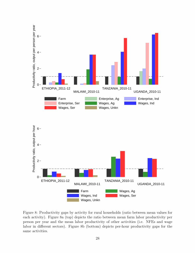
0

2

4

6P

rodu

ctiv

ity r

atio

, out

put p

er p

erso

n pe

r ye

ar



Farm Enterprise, Ag Enterprise, IndEnterprise, Ser Wages, Ag Wages, IndWages, Ser Wages, Unkn

0

2

4

6

Pro

duct

ivity

rat

io, o

utpu

t per

hou

r



Farm Wages, AgWages, Ind Wages, SerWages, Unkn

Figure 8: Productivity gaps by activity for rural households (ratio between mean values foreach activity). Figure 8a (top) depicts the ratio between mean farm labor productivity perperson per year and the mean labor productivity of other activities (i.e. NFEs and wagelabor in different sectors). Figure 8b (bottom) depicts per-hour productivity gaps for thesame activities.

28

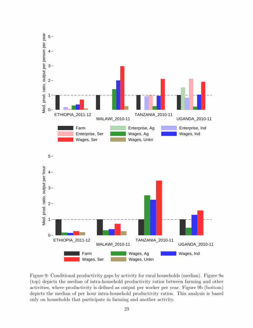
0

1

2

3

4

5

Med

. pro

d. r

atio

, out

put p

er p

erso

n pe

r ye

ar




0

1

2

3

4

5

Med

. pro

d. r

atio

, out

put p

er h

our



Farm Wages, Ag Wages, IndWages, Ser Wages, Unkn

Figure 9: Conditional productivity gaps by activity for rural households (median). Figure 9a(top) depicts the median of intra-household productivity ratios between farming and otheractivities, where productivity is defined as output per worker per year. Figure 9b (bottom)depicts the median of per hour intra-household productivity ratios. This analysis is basedonly on households that participate in farming and another activity.

29

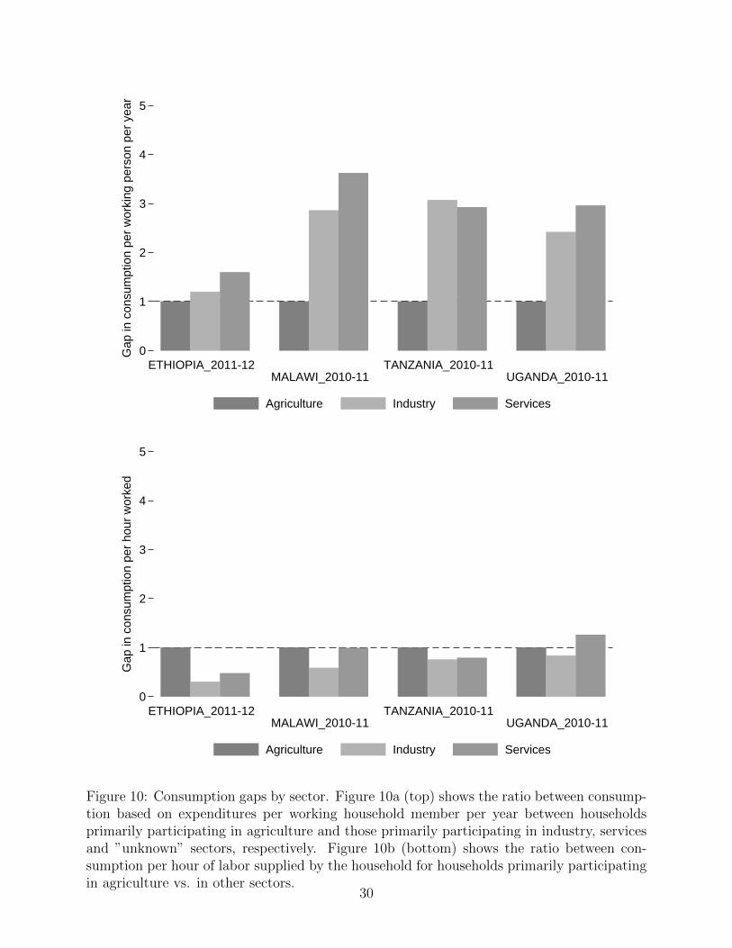
0

1

2

3

4

5

Gap

in c

onsu

mpt

ion

per

wor

king

per

son

per

year



Agriculture Industry Services

0

1

2

3

4

5

Gap

in c

onsu

mpt

ion

per

hour

wor

ked



Agriculture Industry Services

Figure 10: Consumption gaps by sector. Figure 10a (top) shows the ratio between consump-tion based on expenditures per working household member per year between householdsprimarily participating in agriculture and those primarily participating in industry, servicesand ”unknown” sectors, respectively. Figure 10b (bottom) shows the ratio between con-sumption per hour of labor supplied by the household for households primarily participatingin agriculture vs. in other sectors.

30

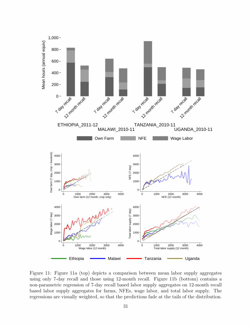
0

200

400

600

800

1,000M

ean

hour

s (a

nnua

l equ

iv)



7 da

y rec

all

12 m

onth

reca

ll

7 da

y rec

all

12 m

onth

reca

ll

7 da

y rec

all

12 m

onth

reca

ll

7 da

y rec

all

12 m

onth

reca

ll

Own Farm NFE Wage Labor

0

1000

2000

3000

4000

Ow

n fa

rm (

7 da

y, c

rop

+ li

vest

ock)

0 1000 2000 3000 4000Own farm (12 month, crop only)

0

1000

2000

3000

4000

NF

E (

7 da

y)

0 1000 2000 3000 4000NFE (12 month)

0

1000

2000

3000

4000

Wag

e la

bor

(7 d

ay)

0 1000 2000 3000 4000Wage labor (12 month)

0

1000

2000

3000

4000

Tot

al la

bor

supp

ly (

7 da

y)

0 1000 2000 3000 4000Total labor supply (12 month)

Ethiopia Malawi Tanzania Uganda

Figure 11: Figure 11a (top) depicts a comparison between mean labor supply aggregatesusing only 7-day recall and those using 12-month recall. Figure 11b (bottom) contains anon-parametric regression of 7-day recall based labor supply aggregates on 12-month recallbased labor supply aggregates for farms, NFEs, wage labor, and total labor supply. Theregressions are visually weighted, so that the predictions fade at the tails of the distribution.

31

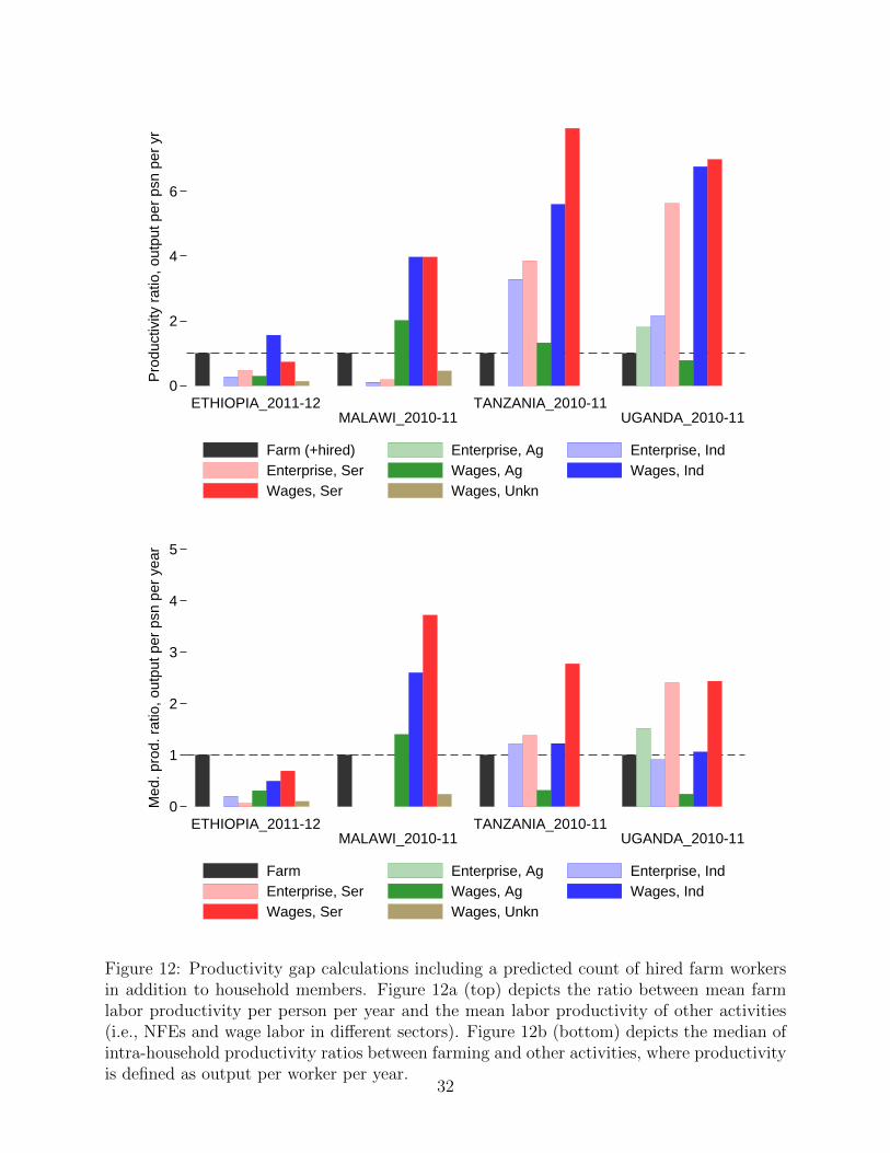
0

2

4

6

Pro

duct

ivity

rat

io, o

utpu

t per

psn

per

yr



Farm (+hired) Enterprise, Ag Enterprise, IndEnterprise, Ser Wages, Ag Wages, IndWages, Ser Wages, Unkn

0

1

2

3

4

5

Med

. pro

d. r

atio

, out

put p

er p

sn p

er y

ear




Figure 12: Productivity gap calculations including a predicted count of hired farm workersin addition to household members. Figure 12a (top) depicts the ratio between mean farmlabor productivity per person per year and the mean labor productivity of other activities(i.e., NFEs and wage labor in different sectors). Figure 12b (bottom) depicts the median ofintra-household productivity ratios between farming and other activities, where productivityis defined as output per worker per year.

32

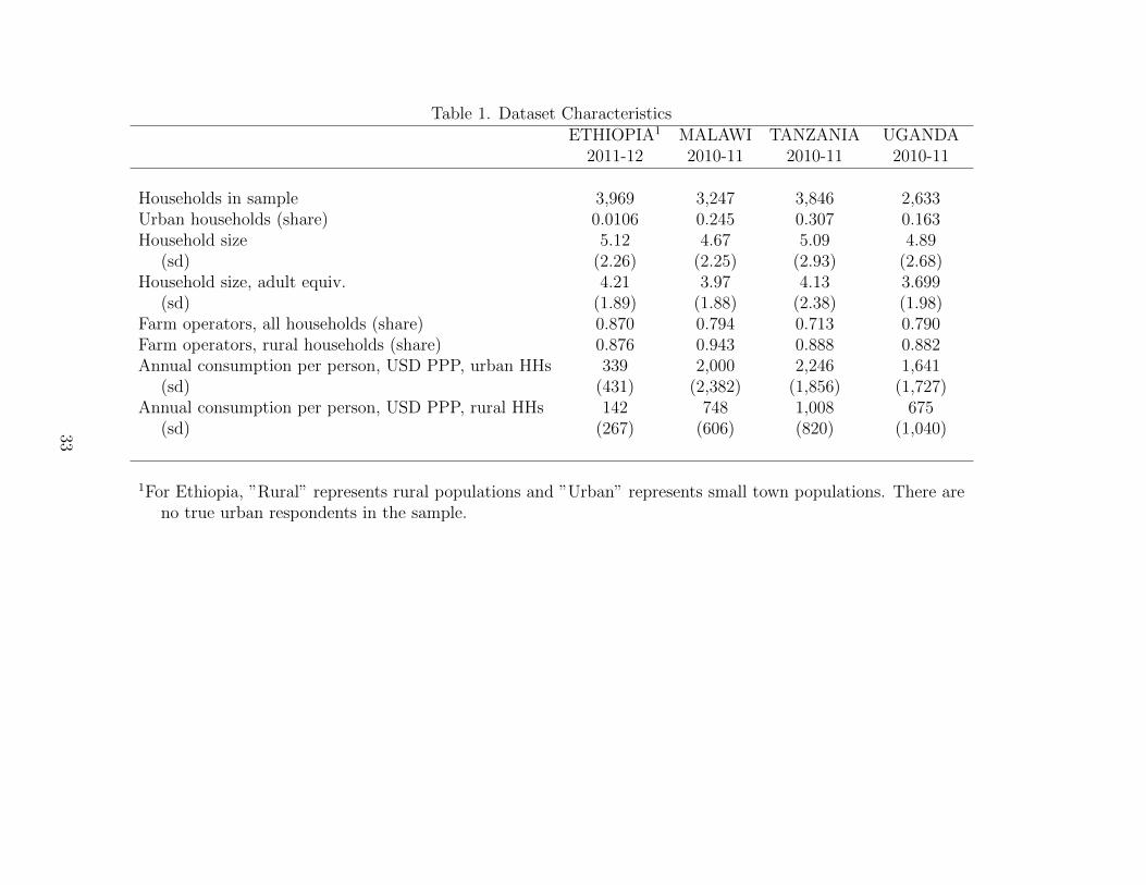
Table 1. Dataset CharacteristicsETHIOPIA1 MALAWI TANZANIA UGANDA

2011-12 2010-11 2010-11 2010-11

Households in sample 3,969 3,247 3,846 2,633Urban households (share) 0.0106 0.245 0.307 0.163Household size 5.12 4.67 5.09 4.89

(sd) (2.26) (2.25) (2.93) (2.68)Household size, adult equiv. 4.21 3.97 4.13 3.699

(sd) (1.89) (1.88) (2.38) (1.98)Farm operators, all households (share) 0.870 0.794 0.713 0.790Farm operators, rural households (share) 0.876 0.943 0.888 0.882Annual consumption per person, USD PPP, urban HHs 339 2,000 2,246 1,641

(sd) (431) (2,382) (1,856) (1,727)Annual consumption per person, USD PPP, rural HHs 142 748 1,008 675

(sd) (267) (606) (820) (1,040)

1For Ethiopia, ”Rural” represents rural populations and ”Urban” represents small town populations. There areno true urban respondents in the sample.

33

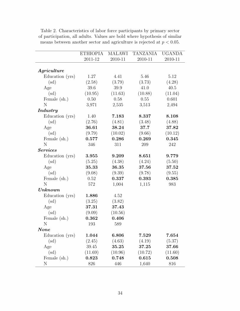
Table 2. Characteristics of labor force participants by primary sectorof participation, all adults. Values are bold where hypothesis of similarmeans between another sector and agriculture is rejected at p < 0.05.

ETHIOPIA MALAWI TANZANIA UGANDA2011-12 2010-11 2010-11 2010-11

AgricultureEducation (yrs) 1.27 4.41 5.46 5.12

(sd) (2.58) (3.79) (3.73) (4.28)Age 39.6 39.9 41.0 40.5

(sd) (10.95) (11.63) (10.88) (11.04)Female (sh.) 0.50 0.58 0.55 0.601N 3,971 2,535 3,513 2,494

IndustryEducation (yrs) 1.40 7.183 8.337 8.108

(sd) (2.76) (4.81) (3.48) (4.88)Age 36.61 38.24 37.7 37.82

(sd) (9.79) (10.02) (9.66) (10.12)Female (sh.) 0.577 0.286 0.269 0.345N 346 311 209 242

ServicesEducation (yrs) 3.955 9.209 8.651 9.779

(sd) (5.25) (4.38) (4.24) (5.50)Age 35.33 36.35 37.56 37.52

(sd) (9.08) (9.39) (9.78) (9.55)Female (sh.) 0.52 0.337 0.393 0.385N 572 1,004 1,115 983

UnknownEducation (yrs) 1.886 4.52

(sd) (3.25) (3.82)Age 37.31 37.43

(sd) (9.09) (10.56)Female (sh.) 0.362 0.406N 193 589

NoneEducation (yrs) 1.044 6.806 7.529 7.654

(sd) (2.45) (4.63) (4.19) (5.37)Age 39.45 35.25 37.25 37.66

(sd) (11.69) (10.96) (10.72) (11.60)Female (sh.) 0.823 0.748 0.615 0.508N 826 446 1,640 816

34

Table 3a. Characteristics of own account and wage workers, Rural adultsETHIOPIA 2011-12 MALAWI 2010-11 TANZANIA 2010-11 UGANDA 2010-11Own Acct Wage Own Acct Wage Own Acct Wage Own Acct Wage

Agriculture (share) 0.826 0.0121 0.887 0.0491 0.818 0.0902 0.744 0.151Hours / year, mean 484.8 1112 281.8 1276 558.6 382.6 532.7 719Share female 0.49 0.209 0.527 0.099 0.529 0.379 0.569 0.493Age, mean 39.43 36.3 39.18 38.39 41.16 39.3 40.65 39.82Educ yrs, mean 1.207 2.597 4.881 6.248 5.498 5.13 5.411 4.616Returns / year (positive), med 1008 382.3 367.1 553.7 329.6 164 244.2 68.88Returns / year (positive), mean 1483 792.6 422.7 967 422.2 513.2 322.9 282.6

Industry (share) 0.0493 0.00887 0.3 0.0344 0.0486 0.0276 0.0331 0.0644Hours / year, mean 1209 1169 770.6 1371 121.1 1138 580.1 908.7Share female 0.601 0.0476 0.532 0.102 0.522 0.176 0.649 0.342Age, mean 37.51 36.62 40.26 37.26 40.35 38.05 40.81 38.3Educ yrs, mean 1.338 3.429 4.83 6.852 6.854 7.656 5.194 6.553Returns / year (positive), med 165.8 733.9 64.09 769 394.3 888.1 242.9 333.6Returns / year (positive), mean 536.6 2445 172.6 1475 949.6 3189 631.1 2048

Services (share) 0.045 0.0267 0.353 0.0642 0.249 0.0846 0.131 0.117Hours / year, mean 1252 1293 1327 1300 236.4 1427 1447 1228Share female 0.564 0.186 0.398 0.205 0.53 0.271 0.415 0.362Age, mean 36.67 35.88 36.39 38.84 39.18 38.81 38.88 39.62Educ yrs, mean 1.694 6.842 6.467 9.79 6.774 9.176 7.408 9.367Returns / year (positive), med 367 1317 128.2 1077 614.8 2049 633.7 929.8Returns / year (positive), mean 1092 1588 262.9 1819 1901 3878 1557 2075

Unknown (share) 0.0136 0.0899 0 0.289 0.000844 0.00187 0 0Hours / year, mean 451.2 362.2 340.1Share female 0.534 0.308 0.462Age, mean 37.91 37.57 37.11Educ yrs, mean 1.754 1.589 4.445Returns / year (positive), med 94.8 76.9Returns / year (positive), mean 223.3 178.1

35

Table 3b. Characteristics of own account and wage workers, Urban adultsETHIOPIA 2011-12 MALAWI 2010-11 TANZANIA 2010-11 UGANDA 2010-11Own Acct Wage Own Acct Wage Own Acct Wage Own Acct Wage

Agriculture (share) 0.184 0.0496 0.285 0.00432 0.259 0.02 0.235 0.0633Hours / year, mean 181.4 112.9 346.9 1016 396.8 503.6Share female 0.553 0.526 0.563 0.321 0.607 0.54Age, mean 39.62 37.59 41.66 36.64 42.07 40.67Educ yrs, mean 3.959 8.223 7.095 5.786 8.28 8.323Returns / year (positive), med 522.9 233 259.4 512.4 143.8 154.5Returns / year (positive), mean 1037 290 337.2 1468 341.7 457.7

Industry (share) 0.171 0.0447 0.104 0.0801 0.08 0.071 0.0462 0.0978Hours / year, mean 1814 1482 1773 1799 148 1653 1530 1319Share female 0.625 0.28 0.377 0.0805 0.414 0.15 0.451 0.235Age, mean 39.88 36.24 36.87 37.08 38.43 36.88 40.75 37.13Educ yrs, mean 3.608 5.708 9.426 10.55 7.608 8.942 9.149 9.797Returns / year (positive), med 220.2 1194 1923 957 2186 464.7 1432Returns / year (positive), mean 521.2 6029 3303 1624 5820 1099 3914

Services (share) 0.197 0.235 0.516 0.26 0.383 0.242 0.239 0.241Hours / year, mean 1904 1644 1799 1844 226.7 2086 2057 1835Share female 0.532 0.315 0.472 0.288 0.585 0.303 0.576 0.422Age, mean 38.68 35.35 34.7 36.74 38.83 37.35 40.54 38.22Educ yrs, mean 3.955 11.7 9.331 11.34 8.17 9.758 9.261 11.89Returns / year (positive), med 224.8 2222 208.3 1999 1300 3074 1521 3186Returns / year (positive), mean 804.9 2539 600.1 5700 3093 5520 2974 5495

Unknown (share) 0.0251 0.0703 0 0.204 0.00254 0.00719 0 0.00306Hours / year, mean 550.7 767.5Share female 0.317 0.263Age, mean 37.63 36.91Educ yrs, mean 5.025 6.8Returns / year (positive), med 159.2 410.2Returns / year (positive), mean 625.1 880

36

Table 4a. Detailed sectors of jobs and enterprises, RuralETHIOPIA 2011-12 MALAWI 2010-11 TANZANIA 2010-11 UGANDA 2010-11Enterprises Jobs Enterprises Jobs Enterprises Jobs Enterprises Jobs

N total (hhs or indivs) 3466 5238 2390 3428 2583 4331 2184 3572of which N part. in firm or job 919 729 441 1354 1044 786 1028 972N firms or jobs 1112 778 469 1415 1404 856 1281 1021

Ag and Primary Prod Share 0.0297 0.0874 0.00853 0.0721 0.0135 0.405 0.117 0.532Mining Share 0.0674 0.00514 0.0107 0.00353 0.0135 0.0152 0.0141 0.00686Manufacturing Share 0.194 0.0206 0.382 0.0269 0.141 0.035 0.244 0.0558Electricity, Utilities Share 0.133 0.00643 0.00212 0.0117 0.00234 0.00392Construction Share 0.0198 0.0244 0.00853 0.0297 0.00712 0.0467 0.00781 0.0725Commerce Share 0.308 0.0116 0.499 0.0155 0.662 0.116 0.39 0.0323Transport, Storage, Comm. Sh. 0.0827 0.00514 0.0277 0.00636 0.0256 0.0397 0.0351 0.0313Finance, Real Estate Share 0.0018 0.00771 0.00212 0.00142 0.0187 0.00156 0.000979Services Share 0.0432 0.158 0.064 0.133 0.131 0.308 0.118 0.254Other Industries Share 0.027 0 0 0Missing sector info Share 0.12 0.647 0.709 0.00427 0.0035 0.0695 0.0108

37

Table 4b. Detailed sectors of jobs and enterprises, UrbanETHIOPIA 2011-12 MALAWI 2010-11 TANZANIA 2010-11 UGANDA 2010-11Enterprises Jobs Enterprises Jobs Enterprises Jobs Enterprises Jobs

N total (hhs or indivs) 503 672 857 1457 1263 2154 746 1227of which N part. in firm or job 293 206 340 657 730 597 440 435N firms or jobs 370 213 409 701 1011 629 584 471

Ag and Primary Prod Share 0.0216 0.0704 0.00489 0.0228 0.0089 0.0461 0.0188 0.0892Mining Share 0.00469 0.00244 0.00143 0.0237 0.0223 0.0137 0.00849Manufacturing Share 0.178 0.0376 0.149 0.0585 0.094 0.0636 0.154 0.0679Electricity, Utilities Share 0.216 0.0235 0.0128 0.00396 0.0143 0.00514 0.0127Construction Share 0.00811 0.0516 0.0122 0.0542 0.0119 0.0715 0.00342 0.0977Commerce Share 0.27 0.0329 0.665 0.0485 0.576 0.205 0.483 0.0764Transport, Storage, Comm. Sh. 0.13 0 0.0562 0.0471 0.0307 0.108 0.0599 0.104Finance, Real Estate Share 0.0329 0.0122 0.03 0.00791 0.035 0.00514 0.00849Services Share 0.119 0.549 0.0978 0.452 0.235 0.421 0.187 0.51Other Industries Share 0.00469 0 0.00198 0.00159 0Missing sector info Share 0.0568 0.192 0.272 0.00593 0.0111 0.0702 0.0255

38

Data Appendix

Table A.1: Wage Labor variable construction notes


Jobtracking

Up to two jobs, ProductiveSafety Net Program (PSNP)

labor, and casual labor

Up to two jobs and casual(ganyu) labor

Up to two jobs

Up to 4 activities including jobs,own farm and NFE (2 most

important in past 7 days and upto 2 more if they are moreimportant over last year)

Time useaggregate

For jobs: months last year; typical weeks / month worked;typical hours / week worked. For casual labor (and PSNP

in Ethiopia): days / last year (hours per day assumed)

Months last year;typical weeks /month worked;hours last week

Months / year; weeks / typicalmonth worked; hours last week

Cleaning(time)

Assume unreported time observation = 0. Truncate unreasonably large values (e.g., >16 hours / day or >7 days /week)

Sector in-formation

Observed for jobs. PSNP isclassified as ag. Casual labor is

classified as “unknonwn”

Observed for jobs. Casuallabor is classified as

“unknonwn”

Observed for bothjobs

Observed for all activities (for4th activity sector is observed

but not whether it is a job,family farm, or NFE)

Wage rateEarnings reported per pay

period (for jobs) and annually(for casual and PSNP labor)

Earnings reported per payperiod (jobs) and per day

(casual labor)

Earnings reportedper pay period

Earnings reported per payperiod (lots of missing pay

period observations)Cleaning(wages)

Winsorize hourly wage rate (p = 0.01) and reconstruct annual returns with imputed wage

Annualreturns

For each job: cleaned wage rate * annual hours

A-1

Table A.2: Farm enterprise variable construction notes (for households involved in crop production)


Seasonsincluded

Only main (meher) season Rainy and dry seasons Rainy and dry seasons First and second seasons

Farm tasksincluded

Post planting (land prep,planting, ridging, weeding,

fertilizer application); harvest

Land prep / planting,pre-harvest; harvest

Land prep; weeding;post planting; harvest

All tasks lumped together

Participation(indiv)

Up to 6 hh membersidentified per task per

plot/task combo

Up to 4 hh members perplot/task combo

Up to 6 individuals perplot/task combo

Up to 3 individuals persubplot

Time useaggregate(indiv)

For each indiv/plot/task:hours / day, days / week,

weeks / season

For each indiv/plot/task:hours / day, days / week,

weeks / season

For eachindiv/plot/task: days

per season (assume 7 hrs/ day)

For each sub-plot: days perseason (assume 7 hrs / day,assume equal labor division

b/w individuals listed)Cleaning(time)

Truncate unreasonably large values (e.g., an individual works more days than the length of the season, or >16hours per day.)

Hired laborFor each plot/task: male,

female and child hiredlaborer person-days

For each plot: male, femaleand child hired laborer

person-days for pre-harvestand harvest periods

For each plot/task:male, female and child

hired laborerperson-days

For each plot: male, femaleand child hired laborer

person-days

Exchangelabor

For each plot/task: male,female and child exchange

laborer person-days

For each plot: male, femaleand child exchange laborer

person-daysNot in survey Not in survey

Farm laborinputs (hours)

Own farm labor + hired andexchange labor (convert to

hours)

Own farm labor + hiredand exchange labor(convert to hours)

Own farm labor (convertto hours) + hired labor

(convert to hours)

Own farm labor (convertto hours) + hired labor

(convert to hours)In all countries, hours supplied by children (age 5-14) are assigned a weight of 0.5

Farm laborinputs (people)

Number of family members with positive hours working on farm (no count of hired or exchange workersavailable). Children (age 5-14) are assigned a weight of 0.5

Annualreturns

Net farm returns are taken from RIGA (see section 2 of paper). Quantity of auto-consumed farm production isestimated using the consumption module of the survey. Net returns are truncated at zero.

A-2

Table A.3: Non-Farm enterprise (NFE) variable construction notes


Participation(indiv)

HH indicates operation ofNFE; up to 5 HH members

can be listed as workers



Indiv indicates whether he/ she is involved in self

employed activities



Time useaggregate(indiv)

Based on 7-day recall inlabor module

For each HH memberlisted as NFE worker:

months / last year; typicaldays / month worked;

typical hours / day worked

Based on 7-day recall inlabor module

Individuals report NFEemployment in labor

module (months / lastyear; typical weeks /

month; hours / last week)Cleaning(time)

Truncate unreasonably large values (e.g., >16 hours per person per day.)

Sectorinformation

Industry code provided inNFE module

Industry code provided inNFE module

Industry code provided inlabor module

Industry codes missing for2/3 of NFEs. They are

predicted using industrycoding from labor module.

Hired laborNumber employees workingfor NFE (past 12 months)

Number of male, femaleand child employees (andhours worked) in a typical

month of operation

Number employees workingfor NFE (past month)

Number employees workingfor NFE (past month)

Firm laborinputs

Can recover number ofworkers (own and hired),

not hours worked

Can recover number ofworkers and hours worked


not hours worked


not hours worked

Annualreturns

Net firm revenues(reported gross sales minus

reported costs)Reported net firm revenues


reported costs)


reported costs)Cleaning(returns)

Reported revenue and cost variables are winsorized (p=.01). Net revenue variable is truncated at 0

A-3

Documents

Labor Productivity and Employment Gaps in Sub · PDF fileLabor Productivity and Employment Gaps in ... This paper is a product of the “Agriculture in Africa—Telling Facts from