Embed Size (px)
Citation preview

Labor Market Search and On-the-Job Learning
in a Growth Model with Human Capital.
Anna Yukhtenko
University of Helsinki
Faculty of Social Sciences
Economics
Master’s Thesis
May 2014

Tiedekunta/Osasto – Fakultet/Sektion –
Faculty
Faculty of Social Sciences
Laitos – Institution – Department
Department of Political and Economic Studies
Tekijä – Författare – Author
Anna Yukhtenko
Työn nimi – Arbetets titel – Title
Labor Market Search and On-the-Job Learning in a Growth Model with Human Capital.
Oppiaine – Läroämne – Subject
Macroeconomics
Työn laji – Arbetets art –
Level
Master’s thesis
Aika – Datum – Month and
year
May 2014
Sivumäärä – Sidoantal – Number of pages
71
Tiivistelmä – Referat – Abstract
In this paper I develop an endogenous growth model with labor market frictions and
spillover effects of physical capital stock on human capital accumulation. Using this
instrument, I study the effects of labor market frictions on the balanced growth path of
the economy, accounting for possible substitutability or complementarity between the
two types of capital. I find out that severe labor market frictions impede economic
growth, lower workers’ wage, educational and work effort. Faster human capital
accumulation process caused by improved market conditions, enhanced importance of
work experience or exogenous positive shocks benefits economic growth. I prove that if
human and physical capital are complements (positive externality), the process of on-
the-job learning increases the speed of human capital accumulation, resulting in higher
work effort and economic growth rate. Substitutability between the two factors of
production (negative externality) leads to inability of workers to adjust to rapid
technological progress, causing economic inefficiencies, invalid usage of capital and, in
the end, lower growth rate of the economy.
Avainsanat – Nyckelord – Keywords
Labor market frictions, economic growth, on-the-job learning, search and matching,
human capital accumulation, physical capital accumulation, substitutability,
complementarity, spillover effect.

Table of contents.
List of symbols 1
Introduction 3
1. Literature review 6
2. The model 9
2.1. Basic assumptions 9
2.2 Firms 9
2.3 Households 12
2.4 Labor market frictions 13
2.5 Consumer good’s market 14
2.6 Human capital accumulation 14
3. Optimization 17
3.1 Basic trade-off relationships 17
3.2 Intertemporal relationships regarding state variables 20
4. Second order conditions 23
5. Balanced growth path 25
6. Comparative statics 32
7. Wage 46
Concluding remarks 51
References 55
Appendix A 58
Appendix B 61
Appendix C 65
Appendix D 69

1
List of symbols.
Factor share of physical capital.
Elasticity of the matching function with respect to
unemployment.
Impact of growth rate of physical capital stock on human capital
accumulation.
Depreciation rate of physical capital.
Measure of convexity of vacancy creation cost function.
Exogenous shift in human capital accumulation process.
Recruitment rate in period t.
Implicit function constructed for work effort.
An employed person’s value of leisure in period t.
An unemployed person’s value of leisure in period t.
Job finding rate in period t.
Subjective time preference rate of a household.
Parameter of an individual’s value function of leisure.
Parameter of an employed individual’s value function of leisure.
Parameter of an unemployed individual’s value function of
leisure.
Number of employees engaged in human resource department
(vacancy creation cost).
Exogenous shift in vacancy creation cost.
Job separation rate.
Household’s preference function over time.
Total factor productivity.
Measure of matching efficiency.
Level of a household’s consumption in period t.
Maximum rate of endogenous human capital accumulation.
Share of an employed individual’s time devoted to education in
period t.
Balanced growth rate.
Growth rate of consumption.
Growth rate of human capital stock.
Growth rate of physical capital stock.

2
Growth rate of output.
Amount of human capital used in production in period t.
The amount of physical capital used in production in period t.
Share of an employed individual’s time devoted to work effort in
period t.
Amount of employees matched with a workplace in period t
Marginal product of factor i.
Marginal valuation of additional human capital in period t.
Marginal valuation of additional employment in period t.
Fraction of employed members in a household in period t.
Effective physical capital-labor ratio in period t.
Ratio of marginal utilities of leisure for employed and
unemployed members of a household.
Rate of return on physical capital (shadow price for capital) in
period t.
Share of an unemployed individual’s time devoted to job search
effort in period t.
U( , , , , ) Household’s felicity level in period t.
u( ) Household’s utility level obtained from consumption in period t.
Number of vacancies in period t.
Real wage on a frictionless labor market.
Wage rate on a frictional labor market in period t
Derivative of function (variable) X with respect to variable
(parameter) i.
Output produced in period t.

3
Introduction.
In 1962 Arthur Okun established the fundamental direct relationship between
changes in unemployment rate and changes in gross domestic product. This
relationship received a name “Okun’s law”, and proved to be true in practice. Indeed,
labor markets are one of the areas that are the most responsive to economic fluctuations.
The crisis of 2008 was no exception. Ever since then, labor markets all over the world
were suffering from severe frictions. Unemployment rates in many countries rose
dramatically; for example, in the USA the number of the employed people declined by
8,8 million in 2009, with 800 thousand jobs lost only in that year’s January, afterwards
reaching its peak of 9,3% in 2010.1 It has been lowered to 6,6% due to active
governmental policy; however, implementing supporting measures required extensive
planning and careful forecasting.
European labor market was also severely influenced by the crisis. The economic
recession created a downward-pushing effect on employment in the whole Eurozone;
between 2008 and 2010 the number of unemployed people in EU-27 rose by 7 million,
resulting in the unemployment rate of 9,7%. Nevertheless, the final outcomes varied
from country to country. The highest unemployment rates were recorded in Greece
(27,8%) and Spain (25,8%), and the lowest ones in Austria (4,9%), Germany (5,1%)
and Luxembourg (6,2%). Nowadays Europe is undergoing a harsh youth unemployment
crisis. In year 2013 across the whole euro area this indicator reached 23,8%. This
happens mostly due to difficulties in finding a job for a young professional.2
All these and many other practical examples prove the importance of labor market
frictions not only for the unemployed, but also for economic development on the whole.
Labor market search is one of the most recent issues these days; many students and
graduates struggle under current economic conditions, ending up working in a field
different from their major or not finding a workplace after all. In my thesis, I analyse the
effect of labor market search and matching frictions on economic growth, taking into
account the importance of education and on-the-job learning.
Another issue discussed in my thesis concerns the dependence between physical
and human capital. World economy changes according to fast technological progress;
expenditure on R&D relative to GDP has risen drastically in many countries all over the
1 U.S. Department of Labor: Bureau of Labor Statistics (2014).
2 Eurostat (2013).

4
world. Northern European countries represent a good example: in Finland 3,87% or
GDP is spent on R&D, in Sweden – 3,42% , in Denmark – 3,06%. Moreover, these
shares tend to increase over time.3
Rapid technological change increases the role of educated workers, motivating
them to increase qualifications and develop new skills. Sometimes new machines are
user-friendly and easy to learn on, which allows a worker to figure out how to operate
them on-the-job. However, in some cases it can be quite hard for an employee to get
used to fast changes in production process. Naturally, successful usage of new
technology has to be facilitated. This can be done in many ways, for instance job
training, qualification courses, mentoring etc.
Taking recent technological development in consideration, I implement the idea
of different effects of physical capital on human capital, aiming to achieve accurate
qualitative explanation and account for various possible outcomes.
In my thesis I use a search model with endogenous human capital and labor
participation developed by Chen et al (2011), extending it by adding the impact of the
growth rate of physical capital stock on human capital accumulation. The latter idea was
borrowed from the paper by Bucci, La Torre (2009). The purpose of the thesis is to
investigate what effects labor market frictions combined with interdependent human and
physical capital accumulation processes have on economic growth. Two possible
interdependencies between the types of capital are taken into account: they can be either
complements or substitutes. I believe that combining these approaches allows
investigating the matter from different sides and reaching realistic results.
In the first part of my work I present the literature on the subjects in the form of a
timeline, introducing various studies concerning search and matching frictions, physical
and human capital and their effects on economic growth. The second chapter explains
the basic assumptions of the model and presents its features. In the next chapter, I
proceed to solving the optimization problem using dynamic programming. After
explaining the first basic intratemporal and intertemporal relationships, I derive second
order conditions in order to prove necessity and sufficiency of existing conditions for
the maximum solution. The fourth part is devoted to equilibrium analysis using
previously derived felicity maximization conditions. Conceptually, the analysis is based
on the balanced growth path.
3 OECD Factbook (2013), 150-151.

5
In the next chapter, the crucial one for the whole thesis, I turn to comparative
statics. I construct implicit functions and take each explanatory variable one by one,
evaluating the effects of various changes in economic conditions on the growth rate,
effective capital-labor ratio and the rate of return on capital. Finally, the last section of
the thesis introduces the difference between the wage derived from my model (with
labor market frictions and on-the-job learning taken into account) and the competitive
(frictionless) wage.

6
1. Literature review.
Labor market frictions started receiving significant attention from economists
relatively short time ago. The first scientific works on the subject were published in the
early 80ies and mainly concerned wage determination under non-perfect market
conditions. However, many fundamental assumptions and results used nowadays were
established at that time.
For example, the paper by Diamond (1982), focusing on the effect of labor market
frictions on wage, introduced the application of the framework of large households to
this matter. The wage there was considered as a function of so-called vacancy rate (ratio
of the number of vacant workplaces to the whole number of jobs in an economy) and
equilibrium unemployment, which gave fruit for thought for many economists later on.
In the 90ies, with rapid development of the Real Business Cycle Theory, labor
market search frictions were implemented into cyclical framework. The classical
examples of this kind of models were introduced by Andolfatto (1996) and Kydland et
al (1991). These papers considered different types of frictions including hours and
employment variations. In both works labor market imperfections were used to explain
the business cycles and fluctuations more efficiently. This somewhat “utilizing”
approach was extensively applied afterwards.4
Nevertheless, the first literature concerning search and marching frictions
appeared only in the early 90ies. One of the most significant works from that period of
time was written by Hosios (1990). He studied the relationship between matching and
unemployment, including various extensions concerning bargaining power and surplus
division. He established the Hosios’s rule, which related a worker’s share of surplus to
his bargaining power. This indicated one of the most important features of many models
studying labor market frictions.
It was not earlier than approximately 10 years ago when labor market frictions
themselves and their effect on economic growth were considered as a separate topic for
research. This rise of attention was mostly triggered by overall critical situation in the
world economy. At that time it seemed crucial to find out the effects of these frictions
on wealth and employment, which, in turn, strongly influence overall economic
development. For example, Mortensen (2004) studied not only the effects of labor
4 For example, Den Haan, Kaltenbrunner (2009) and Matheron, Maury, Tripier, (2004)

7
market frictions on growth and employment, but also possible effectiveness of various
policies that could improve situation on labor markets. In addition, Pischke (2005) paid
special attention to labor market institutions and the way they could influence the
frictions and possibly mitigate them.
Nowadays lots of scientific literature studies labor market frictions, namely
different types of search and matching technologies and frameworks, their effect on
economic development and growth. Various types of additional features are
implemented. For instance, Garcia and Sorolla (2013) include frictional and non-
frictional unemployment, Chen et al (2011) add human capital accumulation and Fujita
and Ramney (2007) investigate the effect of exogenous shocks under frictional
framework.
In my thesis, as it was stated in the introduction, I will also study labor market
frictions and their effect on growth, but with additional features regarding capital
accumulation.
The relationship between physical capital accumulation and economic growth was
established long ago. The fundamental model of exogenous growth was developed by
Solow and Swan (1956), which links economic development to physical capital
accumulation. Human capital did not receive that much attention from scientific word at
that time; labor input was characterized by its quantity and population growth rate was
assumed to be contestant and exogenously given.
The new step in the growth theory was done then by Romer (1994), who
endogenised growth by connecting it to research and development, which lead to
technological progress. Human capital plays a significant role in this new type of
endogenous growth models; by accumulating knowledge and improving education
individuals contribute to the constant growth rate of the economy. Since then, human
capital, its accumulation and effect on economic growth have been actively discussed in
various literature using different approaches, which concerned not only quantitative, but
also qualitative improvements in human capital.5
Nowadays both types of capital are considered as growth factors. Scientists and
researchers try to account for the dependencies between the two, based not only on
research and development, but also on on-the-job learning and positive externalities. For
5 For example, Barro (2001).

8
example, Acemoglu and Angrist (2001) study positive externalities that arise with the
improvement of schooling systems especially in developing countries; Nagypal (2007)
explains the differences between the effects of learning-by doing and matching
efficiency; Alvarez Albelo (1999) analyses the complementarity between physical and
human capital, linking it to convergence and the speed of growth; Bucci and La Torre
(2009) account also for the substitutability between the two.
In my work I combine these two important factors of economic growth under
search and matching frictions. The basic framework of the model is adopted from Chen
et al (2011), who consider a human-capital based growth model with labor market
frictions. However, they do not account for possible effect of physical capital, which
can be either positive or negative, depending on the type of relation between human and
physical capital stocks. As it was stated in the introduction, I extend their model by
adding the spillover parameter which represents the influence of physical capital on
human one. Significant amount of literature reviewed above allows me to conduct
detailed analysis of determinants of economic growth and various factors of influence
under these new assumptions.

9
2. The Model.
In this section I will present the specification, the main assumptions and features
of the model. Firstly, I go through the basic assumptions. Secondly, describe the two
theatres of economic activity – firms and households. After that I explain the set-ups on
the labor market and on the consumer goods’ market. The last part of this section is
devoted to the specification of human capital accumulation process, paying special
attention to the main parameters and variables that are going to be crucial for further
analysis.
2.1 Basic assumptions.
The fundamental assumptions of the model are the following:
discrete time;
closed economy;
continuum of independent infinitely lived firms;
continuum of independent infinitely lived households;
every economic agent is perfectly rational and there is no uncertainty about the
future;
two productive factors – capital and labor, both supplied by households;
firms and households exchange goods and factors of production;
Walrasian goods’ market;
perfect capital market;
frictional labor market (in particular, search and entry frictions).
Each individual has to allocate available time between job search, leisure, learning
or working effort, with the latter two applying only to employed members. In turn, each
firm decides upon the number of vacancies, accounting for the fact that vacancy
creation is costly.
2.2 Firms.
In period t, a representative firm rents capital ( ) at a rental rate ( ), which it
takes as a given. It is useful to note that is equal to the shadow price of capital,
because capital markets are perfect. A firm also employs labor ( ), pays workers
engaged in production real market wage ( ) and produces output ( ) by a Cobb-

10
Douglas technology. Employees that are used in production process exhibit a certain
level of work effort, ( ).
In order to consider also firms’ side of hiring process, one has to account for
vacancy creation costs. Certain studies as, for example, Fujita and Ramney (2007)6,
propose that this type of costs are sunk, which results in a lag between an exogenous
shock and the response of labor market tightness. Another idea of expressing costs of
vacancies is assuming their linearity - in a number of papers, for the sake of simplicity,
it is suggested that there is a linear dependence between the number of vacancies and
their cost.7 I, however, decide to follow Chen et al (2011) and assume a convex,
exponentially increasing vacancy creation cost function. Indeed, in reality posting and
maintaining additional vacancies becomes more and more expensive; a higher number
of vacant places, a need to supervise them, conduct interviews, deal with all
corresponding paperwork requires a larger human resource department. In addition,
workers employed in this unit also have to be paid, in spite of not creating actual
additional value either for the firm or for economy on the whole. One may argue, of
course, that successful matching and productive work are closely connected with the
effectiveness of the hiring process. However, including this into the model would be
unnecessary and may overcomplicate the analysis.
Accounting for vacancy creation costs, as Chen et al (2011), I assume that not the
whole mass of workers in a representative firm is used in actual production of
consumer’s goods8. In turn, a certain number of employees are engaged in so-called
human resource department: they conduct necessary paperwork, maintain the office
space, deal with recruitment processes, qualification improvement, job trainings,
salaries’ payments etc. This measure of human resource department represents the cost
of vacancy creation and has the following form:
, (1)
where , . In this expression, is the number of vacancies, represents
vacancy creation cost, accounts for exogenous shifts in this cost and reflects the
convexity of the cost function.
6 Fujita, Ramney (2007), 3684.
7 For example, Matheron, Maury, Tripier (2002), 1907.
8 Chen, Chen, Wang (2011), 135.

11
Consumption goods are produced according to a Cobb-Douglas technology with
constant returns to scale:
[( ) ]
, (2)
where , . Bucci and La Torre (2009)9 suggest that parameter is equal
to unity. They justify it by referring to omission of disembodied technological progress
and simplification of the analysis. I do not find in necessary in the model under
consideration - works here just as a parameter and its change over time is not
considered in steady-state analysis. In this expression represents the amount of
capital used in production, denotes the amount of employees used in actual
production process. In this particular functional form, the measure of production
workers is augmented by working effort ( , the level of which they are free to choose
and human capital , the accumulation process of which also depends on
households’ decision. So, the effective labor used in production is represented by
. indicates production technology’s parameter (total factor
productivity) and together with denote factor shares of physical capital and
labor, respectively. can be also thought of as the output elasticity of capital. Effective
capital-labor ratio in this case is given by
. (3)
As it was stated above, a representative firm pays a real interest rate ( ) while renting a
certain amount of physical capital from a household. Consequently, the shadow price of
capital (the rate of return on physical capital) can be computed in the following way:
(
)
. (4)
Due to the fact that it’s obvious that the rate of return on physical capital is a
decreasing function of effective capital-labor ratio .
Obviously, there is a direct connection between the shadow rate of return on
capital and endogenous balanced economic growth rate. As suggested by Chen et al
(2011)10
, it is beneficial for further analysis to express effective capital-labor ratio
through the shadow price of capital:
9 Bucci, La Torre (2009), 18.
10 Chen, Chen, Wang (2011), 136.

12
(
)
.
(5)
It is useful to note that in this model wage is endogenous. This feature will be
used in the chapter 7, where I will investigate the effect of frictions on wage.
2.3 Households.
A representative household consists of a continuum of members, which are either
employed or unemployed with fractions and , respectively. Taking into
account each member of a household separately and studying his behavior will
excessively complicate the analysis. In order to avoid this it is useful to implement the
idea of a large household proposed by Lucas (1990)11
. In his paper he accounts for the
possibility of trade between households, assuming that members may have different
features, but at the same time treating them as a united mechanism. This scheme may be
applied to this model too.
On one hand, every household is thought of as a solid unit, with the sum of its
members equal to unity. This assumption allows me to omit unnecessary distributional
and allocational issues that may arise within a household. On the other hand, its
members may be of two types – employed and unemployed, which have different
characteristics.
Employed members of a household have to choose between work effort ,
learning effort and leisure . Correspondingly, unemployed ones face the
problem of division of their time between job search effort and leisure .
There is no on-the-job searching in this model. A household as a separate economic unit
has certain income, and the felicity function of a representative unit of this kind covers
the benefits of all members. All people within a household pool their consumption ,
obtain utility from it and get additional benefits from leisure. Periodic felicity function
for a representative household takes the following form:
, (6)
where u, and
are strictly increasing and concave.
It is worth mentioning that functions and
are different, because employed
and unemployed individuals don’t value their leisure identically. Obviously, the
11
Lucas (1990), 240.

13
unemployed assign less value to free time simply because they are not taking it
voluntarily in most cases. Precise forms of functions appearing in (6) will be specified
afterwards. Economic agents in this model live infinitely, therefore, a household’s
preference over time has a usual form:
Ω = ∑ (
)
,
(7)
where reflects exogenously given subjective time preference rate of a household.
2.4 Labor market frictions.
In order to account for search and entry frictions, matching function has to be
specified. I decided to adopt classic approach proposed by Diamond (1982), where
successful number of matches is conditional on labor market tightness, namely, the
number of vacancies and the mass of the unemployed.12
Although the borrowed
functional form was based on the data from the USA, its origin will not bias further
analysis. So,
= B
, (8)
where , measures matching efficiency and accounts for the amount
of employees matched with a workplace in period t. It is necessary to pay attention to
the parameter – the elasticity of the matching function with respect to unemployment
(search effort taken into account). This parameter reflects so-called “weight” of an
employee in the matching process. It can be also thought of as a measure for the
bargaining power of an employee when it comes to signing a job contract.
Essentially, workers on labor market are not only finding jobs; there is always a
possibility to be fired from the workplace one already has. Therefore, the job separation
rate has to be taken into account. In this model it is exogenous and denoted by It
has the same intuitive meaning as the probability of job separation which is used, for
example, by Den Haan and Kaltenbrunner (2009).13
Furthermore, I specify firms’
recruitment rate
and workers’ job finding rate
. Thus, employment
evolution equation is:
, (9)
which, in turn, can be written in the following form:
12
Diamond (1982), 221. 13
Den Haan, Kaltenbrunner (2009), 314.

14
= (1 – ψ) B
. (10)
Intuition behind (10) is straightforward. The fraction of employed people in period t+1
consists of existing employees that “survived” through job separation (the first term on
the right side of (10)) plus the new workers that have just been matched and hired (the
second term on the right side of (10)).
2.5 Consumer good’s market.
For simplicity, I assume that there is only one consumer good in the model, the market
of which is Walrasian. Therefore, the equilibrium condition of market clearing requires
that the supply of this good is equal to the demand for it:
, (11)
where is exogenously given depreciation rate of physical capital. The left-hand
side of (11) represents households’ demand for the good, which equals to the sum of
pooled consumption and investment in physical capital. The right-hand side of the
equation is, correspondingly, the supply of this only good in the economy (the
production function).
2.6 Human capital accumulation.
The issue regarding the interdependencies between physical and human capital
has been actively discussed in the scientific world. Significant amount of studies pay
more attention to human capital and its role in economic growth, arguing that economy
grows faster if the ratio of human to physical capital is higher.14
But in recent time there
appeared a trend towards coming back to closer analysis of physical capital and its
influence on economic development (of course, combined with human capital).
Following this new trend and pursuing the goal of accounting for two types of
capital in one model and their effects on each other, I extend Chen et al (2011) and
construct the following human capital accumulation equation:
- γ ) , (12)
where represents exogenous shifts in the speed of human capital accumulation
process; accounts for the maximum rate of endogenous human capital
accumulation, which takes place when there is full employment in the economy and all
14
For example, Barro (2001), 16.

15
workers exhibit maximal educational effort; Chen et al (2011) refer to the latter two as
“policy parameters”, the values of which can be effectively influenced by authorities.15
Finally, reflects the impact of the growth rate of physical capital stock on
human capital accumulation. This parameter γ is of special interest; in fact, it will play a
significant role in further analysis. It can be called a spillover effect of physical capital
growth or a measure of learning-by-using. The idea of this spillover parameter was
introduced into a discrete time framework by Bucci and La Torre (2007).16
The intuition is the following. It’s not a secret that many enterprises, especially
ones that use high-tech machines and computers, may experience some difficulties in
actual usage under rapid technology change. Changes can be so quick that an average
worker may not be able to keep up with them. Simply said, it’s not enough to buy the
computers, but it is also necessary to train people how to use them. This may contribute
to the accumulation of human capital, speeding it up and motivating employees to
improve their qualification. However, there is also a possibility that it will lead to a
faster depreciation of human capital (the erosion effect).
Logically, if , the erosion effect takes place and the rapid growth of physical
capital hampers human capital accumulation (physical and human capital are
substitutes, new machinery it too complicated for the workers, they cannot acquire
necessary skills fast enough); in other words, there is a negative externality generated by
fast technological change. If , then faster renovation of physical capital leads to
faster human capital accumulation (physical and human capital are complements,
workers easily learn how to use new technology on the job), creating a positive
externality. It is also necessary to explain the restriction . This inequality
prevents the model from exploding (if ) and human capital stock in period t+1
from being negative (if ). Both situations will lead to unrealistic outcomes.
It is also useful to note that, if , the growth rate of physical capital stock
does not affect human capital accumulation process and the model becomes the same as
the one developed by Chen et al (2011). In this situation human and physical capital are
treated as completely independent factors of production. This idea doesn’t allow me to
look into one of the crucial issues of my thesis – examining possible effects of different
15
Chen, Chen, Wang (2011), 138. 16
Bucci, La Torre (2009), 19.

16
types of interdependencies between human and physical capital on economic growth.
Therefore, I do not elaborate the case of in my work.
No doubt that the value of parameter will have an impact on the balanced
growth rate of the economy. It is exactly this feature of that makes this extension so
important. Unlike Alvarez Albelo (1999)17
, who assumed that physical capital can
exhibit only positive externalities for human capital, this model allows accounting for
two possibilities, the existence of which is proved in reality.
Over past 10 years technology’s impact on economic growth has been extensively
researched and widely discussed. For example, in 2011 during annual Techonomy
conference in New York it was one of the hottest topics. Many scientists and
economists have now agreed upon the fact that too fast technological change may
sometimes be harmful for economy on the whole. Indeed, rapid progress in hi-tech
industry does not necessarily mean that the well-being of workers will increase. On the
contrary, over past years productivity growth in many countries has been quite
moderate. As technology escalates, there appears a need to change existing institutions
and improve skills, which in many cases turn out to be difficult. This model allows
analysing these interesting two-sided effects.
17
Alvarez Albelo (1982), 358.

17
3. Optimization.
The first problem to be addressed is, naturally, the optimization problem. As there
are two types of economic agents (firms and households) which influence each other’s
choices while pursuing similar goals – profit and felicity maximization, it will be logical
to use dynamic programming method to figure out optimality conditions. This will
allow accounting for the flows of different variables and several budget constraints and
avoid unnecessarily long Lagrangians.
In this part of the thesis I present the optimization problem, provide first-order
conditions and explain the first results - basic intertemporal and intratemporal trade-off
relationships that govern the behavior of firms and households according to their aims.
In order to obtain more complicated intertemporal relationships that explain the
evolution of human capital and employment as well as the allocation of a household’s
income between consumption and saving, I use Benveniste-Scheinkman conditions.
They are also often referred to as Envelope theorem. Their usage can be justified by the
fact that they simplify the analysis. In particular, Benveniste-Scheinkman condition
states that the change in the maximal value of the function as a parameter changes is the
change caused by the direct impact of the parameter on the function, holding other
variables constant at their optimal values. This property is used regarding physical
capital ( , human capital ( and employment level ( . Resulting equations will be
useful afterwards for obtaining balanced growth equilibrium values and further analysis.
3.1 Basic trade-off relationships.
As it was said before, I will solve the optimization problem using dynamic
programming, namely Bellman equation. Throughout the whole thesis, I will focus on
two representative periods – t and t+1, which can be done without biasing the result.
The problem can be specified as:
(13)
subject to constraints (10), (11), (12). It is useful to note that in this case only one value
function is maximized. It accounts for the well-being of both firms and households at
the same time. Some studies suggest different approach, examining the theatres of

18
economic activity separately.18
Bucci and La Torre (2009) propose paying more
attention to households’ decision, because in the end it is the household that consumes
goods produced by a firm.19
Nevertheless, I decide to follow Chen et al (2011) and use
the classical approach of dynamic programming and construct one value function.20
In order to simplify the notation, I denote the vector of variables ( ) as ,
and vector or the same variables from period t+1 ( ). as . From now
on, I will omit subscript “t” for all variables from period t and denote the ones from
period t+1 with subscript “+1”.
The first-order conditions of the specified problem with respect to consumption
( ), work effort ( , learning effort ( , search effort ( and the number of vacancies
( are, respectively:
,
,
,
,
.
Solving these first-order conditions results in (14) - (18):21
, (14)
( ) , (15)
, (16)
, (17)
. (18)
Then let me denote the marginal valuation of additional human capital in the next
period (in this case t+1) as
. Correspondingly, the marginal valuation
18
Matheron, Maury, Tripier (2002), 1906-1907. 19
Bucci, La Torre (2009), 21. 20
Chen, Chen, Wang (2011), 139. 21
See Appendix A for details.

19
of additional employment for next period will be
. Using this new
notation, I can write the first result – intratemporal and intertemporal trade-off
relationships, that represent the first step in the analysis.
( ) , (19)
, (20)
, (21)
. (22)
(19) was obtained by combining (14) and (15). This reflects a trade-off between
consumption and work effort. Namely, the marginal rate of substitution between the two
(right hand side) is equal to the marginal product of labor (left hand side). For every unit
of consumption an individual would like to have, he has to work additional time. He
makes his choice according to utility gain from increasing consumption and utility loss
from being more active at work. Simply said, equation (19) governs decision whether to
work or not to work.
(20) originates from rearranged (16). Here, measures human capital
accumulated through learning, as a result of putting a certain effort into this activity.
Indeed, coming back to equation (12), it is obvious that if a worker decides to exhibit
more learning effort, represents the direct effect from this addition. In a way,
may be thought of as a multiplier that reflects the effect of a rise in educational effort.
From (20) one can infer that marginal disutility from devoting additional effort to
learning should be equal to the marginal valuation of human capital acquired through it.
As far as stable equilibrium is concerned, this intuition is perfectly logical.
Plugging the expression for the marginal valuation of additional employment into
(17), I get (21). This one has a similar logic to the latter expression. On the one hand,
more active search effort (hence, a drop in ) results in an increase in
employment, which should be beneficial for a household; on the other hand, an
individual experiences utility losses from reducing his leisure by devoting more time to
job search. In the equilibrium, (21) holds and equates the marginal disutility from
putting a larger share of time into search to the marginal value of the following increase
in employment.

20
Performing similar to the latter substitution procedure and then plugging (14) into
(18) yields (22).22
This expression reflects a slighter different concept. Here, the left
hand side represents marginal addition to the employed pool by posting another
vacancy, and the right hand side reflects the marginal size of labor that should be moved
from production to human resource department in order to maintain these new
vacancies. This statement describes another important equilibrium condition of the
model. It takes into account the production gains from additional worker and the costs
of employment procedure, both of which are encountered by a producer.
3.2 Intertemporal relationships regarding state variables.
Now the goal is to obtain more complex intertemporal relationships and continue
with the analysis towards the balanced growth path. As it was justified before, I use
Benveniste-Scheinkman conditions regarding so-called state variables :
, (23)
, (24)
(25)
Equations (23)-(25), after rearranging and plugging in expressions for
,
,
,
,
,
result in:
, (26)
( )
,
(27)
.
(28)
Now I have everything needed to derive important intertemporal relationships that
were mentioned before. Firstly, using (14) in (26) I get:23
(29)
22
See Appendix A for details. 23
See Appendix A for details.

21
Obviously, the left hand side of (29) represents the marginal rate of substitution
between consumption over time, while the right hand side is the rate of return on
capital. The equation accounts for a very important issue in this model, namely, the
relationship between consumption and saving. Incentives to make the decision of saving
for the next period depend positively on the rate of return that can be received
afterwards as the result of reducing consumption in the current period and increasing the
savings.
Secondly, multiplying both sides of (27) by and rearranging it gives:
( )
(
) .
Using previously derived expressions for and from (15) and (16) as well as
noting that the marginal valuation of human capital today is , I rewrite
the preceding equation as:
(
).
(30)
(30) describes the evolution of human capital over time, stating that it depends not
only on learning but also on working effort. In order to become more educated, one has
to give up an arbitrary fraction of his time devoted to work effort and/or leisure. Also it
can be seen that – the measure of the effect of the growth rate of physical capital on
human capital accumulation – appears in this equation. The growth rate of physical
capital stock ( ) will have a certain influence also on the marginal valuation of human
capital in current period; however, the final effect is still conditional on the sign of . If
, so that physical and human capital are substitutes, an increase in it will decrease
. Indeed, in practice, human capital may become less valuable due to its faster
depreciation. If , meaning that both factors of production complement each other,
its presence may positively affect the marginal value of additional human capital in
current period. It can be explained simply by the positive spillover effect created by the
physical capital – for example, installing modern machinery that is easy to learn on
(hence, increase the level of human capital) will definitely make a positive contribution
to the value of human capital.
Thirdly, after multiplying both sides of (28) by and rearranging the equation I
obtain:

22
( )
.
Analogously with the previous case, using formulas for , and from (15),
(16) and (17) combined with remembering that , the latter equation can
be transformed into:
. (31)
(31) describes the evolution of employment over time. In this model the marginal
value of employment depends on four factors:
Additional utility received by a household after another member of it finds a job.
The higher is the additional utility from another employed member of a
household, the higher is the marginal value of employment.
Disutility from work. Indeed, if utility losses faced by a representative
household’s member are high, the marginal valuation of employment will be
relatively low; therefore, there will be lower incentives to enter the labor market.
Disutility from learning effort. Higher educated workers are more productive
and can bargain about higher wages, which seems to be beneficial for a
household; but if disutility from learning effort is too large (for example, high
tuition fees, transportation and opportunity costs, low educational abilities of
individuals that decide to study), a household will not be able to benefit a lot
from additional employment.
Disutility from search effort. Obviously, if job search is costly and exhausting,
even a successful match resulting from it will not bring significant addition to
household’s felicity level.
Another important issue was mentioned by Chen et al (2011). Analysing equation
(31), one must note that if employed members value leisure more than unemployed,
there is a possibility that increase in marginal utility from leisure (as the result of
additional employed member) may decrease the marginal value of employment for a
representative household.24
24
Chen, Chen, Wang (2011), 140.

23
4. Second order conditions.
To provide the proof for the existence of the maximum, I consider second order
conditions. In order for a function to have a relative maximum at a point where its
derivative with respect to a variable in question is equal to zero, second order derivative
at this point should be negative. Using first-order conditions later in the thesis I will
derive the balanced growth equilibrium. I shall prove its existence step by step, using
second order conditions.
Firstly, substituting expression for the marginal product of labor
( ) in (15) gives
. (32)
The marginal product of labor is positive according to concavity assumption
regarding production function. Rearranging the latter equation proves the following:
.
(33)
By applying the functional form of vacancy creation cost function it can be shown
that the marginal product of human capital equals:
( )
,
so that
( )
[ ( )
] .
Then, by plugging the expression for into (18),
. (34)
Also I will need previously specified firms’ recruitment rate
and workers’ job finding rate
.
Now I will prove that second order conditions are met, therefore, there exists a
maximum solution to problem addressed in my thesis.
Using (33) in (14) and differentiating it with respect to c results in

24
, (35)
due to the concavity of function. Therefore, and the second order condition
with respect to consumption is met.
Taking the derivative of (32) with respect to yields
. (36)
Again, due to concavity properties, and . Therefore, .
Hence, the second order condition with respect to work effort is met.
Performing similar procedure for (16) results in
, (37)
which proves that the second order condition with respect to educational effort is met.
Plugging expression for into (17) and taking the derivative of the latter with
respect to gives
( )
, (38)
because due to its concavity and . Therefore, the second order
condition regarding search effort is met. 25
The last condition to be checked refers to the number of vacancies. Inserting
expression for (34) and differentiating it with respect to results in
(39)
Therefore, the last second order condition is met.26
So, based on (35) – (39), I have proven that (14) - (18) and also (29) - (31) are
necessary and sufficient conditions for the existence of the maximum solution.
25
See Appendix A for details. 26
See Appendix A for details.

25
5. Balanced growth path.
As it was stated before, equilibrium analysis will be based on the concept of
balanced growth path (BGP, afterwards). On this path output, consumption, physical
and human capital grow at the same rate. In this section I will use previously derived
equilibrium conditions that originate from felicity maximization problem.
For further discussion it is necessary to specify the functional forms of ,
and
. Again, for simplicity, I omit subscript “t”. Chen et al
(2011) suggest the following functions: 27
utility function: ,
an employed person’s value of leisure:
,
an unemployed person’s value of leisure:
,
where , are positive parameters and ≠1. In the end, the felicity function of a
household looks like this:
. (40)
All three functions included in (40) are concave. and
for employed and
unemployed members of a representative household are of similar form, but have a
different parameter of leisure valuation . Intuitively, I propose that employed people
value their leisure more than unemployed, . Indeed, taking into account that the
employed have a somewhat more difficult choice concerning time division (they have to
decide between three alternatives: work, learning or leisure) than the unemployed, it is
logical that the latter will value leisure less than the former. Moreover, as it was
mentioned before, an unemployed person may find himself in this position
involuntarily, e.g. due to job cuts.
For analytical reasons the ratio of marginal utilities of leisure for employed and
unemployed members of a household is denoted by
.
The analysis will be conducted by constructing, using and explaining the balanced
growth path (BGP) of the economy. The equilibrium itself consists of the values of
variables (output), (consumption), (work effort), (educational effort), (job
27
Chen, Chen, Wang (2011), 142.

26
search effort) and (the number of vacancies), (physical capital stock), (human
capital stock), (employment) together with (the number of matches on the labor
market), (effective capital-labor ratio) and (the rental rate for physical capital,
which is equal to the rate of return on physical capital). Along the balanced growth path
consumption, output, human and physical capital grow at the same rate. I denote this
rate by .
It is useful to note one feature of the model that will be extensively used later.
One may think that the assumption of equal growth rates of physical and human capital
will lead to a dead end in the analysis because one of the key propositions was that the
growth rate of physical capital stock is included into human capital accumulation
equation. These doubts will be proven wrong in my thesis. The interdependence
between the two growth rates will be taken into account in the analysis. Moreover, it
will be shown that depending on the type of the relation between physical and human
capital (complementarity or substitutability), the effect of this interdependence on the
BGP values of key variables will be different.
Dynamic equilibrium requires that the following conditions are met:
intertemporal and intratemporal optimization equations (19)-(22) and (29)-(31)
are binding,
production function has the form of (2),
human capital evolves according to (12),
accumulation equation for employment is given by (10),
effective capital-labor ratio is represented by (5),
matching process on the labor market occurs according to (8),
goods’ market clearing condition (11) holds.
Now I turn to the analysis of the balanced growth path. Noting BGP’s key feature
of the common growth rate, I rewrite human capital accumulation equation (12) as:
,
which can be rearranged to get:
. (41)
The interpretation of this result is rather intuitive. Obviously, learning effort
depends positively on the economic growth rate, negatively on the employment rate (the
27
more employed people there are, the less education is needed, no need to increase
qualification in order to get a job etc.) and also negatively on exogenous shifts in the
speed of human capital accumulation process and the maximum rate of endogenous
human capital accumulation . The latter negative relationships can be explained by
looking at the human capital accumulation equation (12). Indeed, it follows from it that
the higher policy parameters or are, the less studying effort is needed to accumulate
human capital. The influence of parameter which is of a special importance in this
analysis, is conditional on the relationship between two types of capital. If physical and
human capital are substitutes , then learning effort increases with an increase in
; workers need to get more education in order to “compete with the machines” and
work productively, adjusting to the new level of technology. On the contrary, if physical
and human capital are complements , workers benefit from physical
capital accumulation, on-the-job learning contributes to human capital and less
additional education effort is needed.
Rearranging goods market clearing condition and applying BGP’s properties, I
get:
( ) ( (
( ) )
( ) (
)),
rewriting which yields:28
( ) . (42)
Next I derive an expression for consumption growth. It follows from (29) and (4)
that
,
which gives a Keynes-Ramsey relationship for consumption growth:29
. (43)
Keynes-Ramsey rule for consumption growth states that the growth rate of
consumption will be positive as long as the interest rate adjusted for the depreciation
rate (the net interest rate ) exceeds the time preference rate . In addition, one
can infer from (43) that the larger is the difference between the net interest rate and the
28
See Appendix B for details. 29
See Appendix B for details.

28
time preference rate, the higher is the growth rate of consumption, which results in a
steeper consumption path.
For the further analysis of the BGP I need to establish the intertemporal
relationships between the marginal valuation of additional human capital and
employment in current and next periods.
Felicity function (40) consists of utility received from consumption and leisure by
employed and unemployed people. It follows from the fact that the functional forms of
and
are weighted by the fractions of the employed and the unemployed, that the
marginal overtime preference of a household with respect to employment level is
constant. In other words, any reallocation of workers from employed to unemployed
and vice versa has no impact on household’s overall felicity level in the long run,
because weights and sum up to 1 in any case. and require
further explanation.
From (14) it can be inferred that
.
According to this, is decreasing in c, therefore, it decreases at the
constant rate . Rearranged equation (20) takes the following form:
.
Keeping in mind that due to the negative effect that additional learning
effort has on utility level, one can state that depends negatively on . It means
that also decreases over time at the balanced growth rate . Based on the
proved properties, the former equations can be rewritten as
, (44)
and
. (45)
And from (17),
. (46)

29
Using (44) - (46), now I can derive another BGP relationship that will connect the
growth rate and work effort, which will be crucial for later discussion. So, plugging (41)
into (30) results in
(
), (47)
and afterwards using (45) and (20) in (47), I get
.
(48)
By applying functional forms to the latter I obtain the final result30:
. (49)
This relationship is derived from human capital accumulation condition and
represents the positive dependence between the economic growth rate and work effort.
In reality, an increase in the growth rate of an economy boosts production, increases
wages, making individuals more willing to put additional effort into productive work.
The same type of dependence applies to the rate of time preference - the higher
individuals value their future, the more they work in the current period.
Another important relationship to be derived is based on employment evolution
equation (31). Inserting functional forms in (31) gives a complicated expression:
.
After transformation and simplification, the latter becomes:
,
which can be further simplified to yield the final relationship:31
[
]. (50)
(50) governs intertemporal employment evolution on the BGP. In other words, it
reflects how employment will be changing over time, taking into account that
consumption, output, human and physical capital are supposed to be growing at the
same rate . In the next section, comparative statics analysis will be done in order to
30
See Appendix B for details. 31
See Appendix B for details.

30
understand what will be the effect of an increase in employment on the balanced growth
rate. This issue is quite ambiguous; so far, common logic suggest that, on one hand, an
increase in employment will increase household income, thereby boosting growth; on
the other hand, it may be possible that an increase in the employment rate will hamper
growth due to an increased in producer’s cost of creating more workplaces.
Another condition that should hold in the equilibrium concerns vacancy creation
and matching. Plugging functional forms into (19) gives:
( ) .
Rearranging this equation results in the following expression which will be used
later:
.
(51)
Coming back to the vacancy creation trade-off and combining (21) with (22)
results in
.
Using (51), the expression for with the mathematical forms of functions in the
latter equation, I obtain
, (52)
which is the relationship in question, the one that is based on vacancy creation trade-
off.32
Logically, equation (52) takes into account not only vacancy creation costs and
their dependence on the number of vacancies, but also the job finding rate, the
recruitment rate and parameter , which can be thought of as power possessed by an
employee when a matching decision is made. Indeed, it is obvious from the (52), that
the higher is this power , the more workers will be hired (the recruitment rate
increases).
The relationship between the rental rate of physical capital and the balanced
growth rate is obtained by simply rearranging (43):
. (53)
32
See Appendix B for details.

31
Inserting (53) into the definition of effective capital-labor ratio (5) yields the last
BGP relationship:
(
)
.
(54)
Relationships (53) and (54) reflect standard logic. The rate of return on physical
capital and effective capital-labor ratio are constant on a BGP. But of course, if an
economy starts growing faster, the rate of return on physical capital will increase which,
consequently, will boost investment.
Summing up analysis performed above, the balanced growth path equilibrium in
this model in characterized by the system of equations (43), (49), (50) and (52)-(54). At
first sight it may appear to be strange that the resulting equations do not have parameter
in them. It can be explained by the fact that in the end the growth rate will be the same
for consumption, output, human and physical capital on the BGP. Nevertheless, it will
be shown in the next section that this common balanced growth rate is affected by
parameter through its effect on work effort.

32
6. Comparative statics.
In this section the comparative statics analysis of the model will be presented and
the key questions of the paper will be tackled. Firstly, I will construct the Beveridge
curve accounting for labor market frictions. Secondly, using it, I will rewrite the
recruitment rate , the number of vacancies and search effort through job finding
and employment rates. This way, the system of equations (43), (49), (50) and
(52) - (54) will be reduced to two-by-two. Thirdly, work effort will be expressed
through several parameters of the model: the job finding rate , the employment rate ,
the degree of matching efficiency , the job separation rate , exogenous shift in
vacancy creation costs , the maximum rate of endogenous human capital accumulation
, exogenous shifts in human capital accumulation and the impact of the growth rate
of physical capital stock on human capital accumulation – namely, vector
After that I will express the balanced growth rate , the shadow
price for physical capital and effective capital-labor ratio through the same vector.
This will allow taking each explanatory variable one by one and analysing their effects
on four dependent variables – work effort, the balanced growth rate, the rate of return
on physical capital and effective capital-labor ratio. In order to do this, implicit function
will be constructed.
As it was stated above, it is necessary to derive the Beveridge curve in order to
establish the relationship between the unemployment rate and the number of vacancies.
In this case it will also connect the job finding rate, the job separation rate, search effort,
matching efficiency parameter and the number of newly matched workers.
The first part of the curve follows from the assumption that the pool of workers
that lost their jobs due to job separation has to be equal to the amount of newly
matched employees in the equilibrium . This, in turn, has to be equal to the
number of vacancies filled at a certain period of time . In addition, all these values
should be equal to the value of the matching function (it also represents the number of
matched people). In the end, I get a “four-sided” Beveridge curve:
. (55)
Based on (55), it will be shown that endogenous variables can be expressed
through the job finding rate and the employment rate . Naturally, using (55), I derive
the following lines:

33
,
.
These formulas allow expressing the recruitment rate through and , with
being an exogenously given matching parameter:
, (56)
with properties
and
. These results
are consistent with real life evidence. Indeed, if matching efficiency increases, this
should lead to an increase in the recruitment rate . And a larger pool of newly matched
workers, as a consequence of an increase in the job finding rate, is followed by a decline
in the recruitment rate.
Using the Beveridge curve and (56), I express the number of vacancies through
endogenous variables , , exogenously given matching efficiency and the job
separation rate :
. (57)
It can be seen from (57) that
,
,
and
. An
increase in matching efficiency will give a push to the labor market, accelerating
matching process and therefore decreasing the number of open vacancies (they get filled
faster). A rise in the job finding rate, as it was said before, will induce a downfall in
firms’ recruitment rate, which in the end leads to a higher number of unfilled vacancies.
As far as the job separation rate is concerned, an increase in it will lead to more empty
workplaces, which results in a higher number of vacancies. Moreover, an increase in the
number of employed people will result in a higher number of newly created vacancies,
because there will arise a need to establish more workplaces.
Another consequence from the Beveridge curve is the following:
. (58)
From (58) it is easy to see that (
)
,
and

34
If the job finding rate is high, it leads to a lower search effort. In this case workers
need not put that much effort into looking for a job, they can simply rely on efficient
matching mechanism. An increase in the quantity of employed workers, on one hand,
decreases the number of workers being matched ( goes down); on the other
hand, it also requires creation of new vacancies. Both of these effects result in higher
job search effort. This phenomenon can also be explained by overall positive effect of
increased employment: members of a household, seeing that the employment rate has
risen, believe that the labor market is in good condition and, therefore, exhibit more
search effort.
Finally, after expressing , and in terms of and , I can start the analysis of
comparative statics. As it was said before, work effort will be expressed through
several parameters of the model, such as the job finding rate , the employment rate ,
the degree of matching efficiency , the job separation rate , exogenous shift in
vacancy creation costs , the maximum rate of endogenous human capital accumulation
, exogenous shifts in human capital accumulation and the impact of the growth rate
of physical capital stock on human capital accumulation . But firstly, I will figure out
the dependencies between the BGP values of work effort , the growth rate , the
shadow price for physical capital and effective capital-labor ratio . Rearranging (49)
defines the relationship between the economic growth rate and working effort:
. (59)
Embedding (49) into (41) yields the following important statement which
represents the positive relationship between educational and working effort on the
balanced growth path:33
. (60)
This can be interpreted intuitively. By definition, output, consumption, human and
physical capital grow at the same rate on the balanced growth path. Therefore, devoting
more time to work effort will result in an increase in output, boosting economic growth.
A more developed economy is likely to use more complicated machinery due to
technological progress; in order to be able to keep up with the higher economic growth,
more educational effort is necessary.
33
See Appendix C for details.

35
From the equilibrium relationship based on vacancy creation trade-off (52), noting
the expression for the ratio of marginal utilities of leisure for the employed and the
unemployed ( ) and rearranging the result, I obtain:
.
(61)
The left hand side of this equation needs to be expressed in terms of the vector of
variables and parameters, according to which further investigation was planned to be
conducted. So, plugging (60) into the left hand side of (61) results in:34
(
)
.
(62)
(62) can be substituted into (59), (53) and (54), resulting in the following
expressions for , and , respectively:
( )
(
)
,
(63)
[
(
)
] ,
(64)
(
[
(
) ]
)
.
(65)
Now I will tackle the key point of the thesis – the demonstration of the
relationships between the variables on the balanced growth path. It is useful to note that
Chen et al (2011) focus only on the balanced growth rate and do not provide detailed
explanation regarding each parameter that I am going to describe.
I will take each parameter one by one and explain its impact on work effort , the
balanced growth rate , the rate of return on physical capital and effective capital-
labor ratio . As seen from (62), in order to obtain the necessary derivatives, implicit
function for has to be constructed. I denote this function by Hence,
(
)
.
(66)
34
See Appendix C for details.

36
Here I will present only the final outcomes and interpret them. The detailed
process of obtaining the derivatives as well the table with summarized results are shown
in the Appendix C.
Job finding rate ( ).
According to the properties of implicit functions, the total derivative of will take
the form of , where subscripts denote partial derivatives. This means
that relationship in question can be computed in the following way:
.
(
)
(
)
(
) ,
(
)
(
) .
The latter derivatives are both positive, which leads to the following outcome:
.
If the job finding rate increases, more matches occur. It follows from equation
(21) that an increase in matches lowers the marginal utility from additional employment
( , in this notation). That will decrease employees’ incentives to put more effort
into work. Indeed, in practise, if a worker knows that in any case it is relatively easy to
find a new job, he will be less motivated to work harder in order to keep the existing
one.
As the balanced growth rate depends positively on work effort, it can be stated
that
. The growth rate will be hampered by an increase in the job finding rate,
because there will be less incentives to work harder and create more additional value.
Moreover, educational effort will be also decreased – as it was written before, a
representative worker feels secure of his future and is not motivated to improve existing
skills. In addition, due to Pareto-complementarity of firms’ and households’ choices, the
marginal benefit of additional employment is lowered.
If it is easier to find another job, a representative worker, logically, will become
more “choosy”, asking for a higher wage and refusing to accept a job with somewhat
less beneficial conditions. That will be highly unfavourable for the firms. Therefore,
effective labor used in production will decreased, producers will try to use more

37
physical capital – effective physical capital-labor ratio ( ) increases, which leads to a
decrease in the rate of return on physical capital ( ).
Employment ( ).
In order to evaluate the effect of a rise in employment on work effort and the
growth rate of the economy, effective capital-labor ratio and the rate of return on
capital,
has to be computed. To do do this, as in the previous case, I derive:
(
)
.
Therefore,
.
Increased employment has an ambiguous influence on work effort. In fact, it
creates two opposing effects. Firstly, it lowers the marginal benefit of employment due
to diminishing returns to scale. Therefore, work effort decreases. Looking into this
question from a realistic side, it seems logical that when there are more employees
engaged in production, there is no need for a representative worker to exhibit more
work effort. Indeed, in this case production tasks are allocated among a larger number
of people, so that each employee has to do less.
At the same time, an increase in the employment rate pushes the marginal benefit
of employment upwards due to Pareto-complementarity of employment and work effort
(this can be inferred from the production function (2)). An increase in employment
means increase in a representative household’s wealth, which creates additional
incentives for investment. That, in the end, fosters work effort. Therefore, the final
result of an increase in employment cannot be stated precisely; the outcome will depend
on which of the two opposing effects dominate.
As far as economic growth is concerned, mathematical results again suggest
ambiguity regarding its dependence on the employment rate. Taking the derivative of
(59) with respect to results in:
.
Taking a closer look at this expression suggests that it will be most probably
positive. The sign of the last term on the right side is unknown, but the first term is
surely positive. Therefore, even though mathematical derivations suggest uncertainty

38
regarding this matter, an upturn in employment will most likely have a positive effect
on the balanced growth rate.
In addition, real life evidence suggests that an increase in employment and,
consequently, a decrease in unemployment have a positive effect on the economic
growth rate. For example, Mortensen (2005) suggests that a higher rate of employment
will “encourage the investments in R&D needed for higher rates of long term growth”.35
In this paper I do not pay special attention to specific R&D activities, but Mortensen’s
proposition gives additional proof for the existence of the positive correlation between
employment and economic growth. Also Chen et al (2011) present in their calibration
results the fact that a rise in employment level creates an upward-pushing effect on
economic growth. The impact induced by diminishing returns to scale is dominated by
the positive effect of employment creation.36
Moreover, in the publication of the
Organisation for Economic Co-operation and Development “Promoting Pro-poor
Growth: Employment” (2009), increasing employment is proved to be one of the main
goals on the way to achieving balanced growth in emerging countries.37
All these facts
support the proposition that an increase in the employment rate is likely to result in a
higher economic growth rate.
Whereas numerical analysis proposes the same uncertainty regarding the last two
variables under investigation, and , intuitive logic suggests
and
. The
impact on effective capital-labor ratio will be negative due to an increase in the number
of employees. As and are negatively dependent, there is a positive effect on the
rate of return on physical capital. The amount of physical capital relative to the amount
of human capital used in production is reduced, which leads to an increase in the rate of
return on physical capital.
Matching efficiency ( ).
Parameter B, earlier specified as matching efficiency, accounts for the severity of
labor market frictions. At first sight this exogenous parameter may not appear to be of
great importance, but in the end it represents one of the crucial features of the model. A
higher results in improved market conditions, meaning that the frictions are more
moderate and matching is more efficient. Computing the partial derivative of with
respect to B yields:
35
Mortensen (2005), 260. 36
Chen, Chen and Wang (2011), 149. 37
OECD report (2009), 41.

39
[ (
) (
) ] ,
keeping in mind the fact that and .
This allows to state:
.
This result is completely clear and rational: indeed, better labor market conditions
and less uncertainty improve overall functioning of an economy, leading to higher work
effort and faster economic growth. The quality of matching will also increase, which
leads to more productive and efficient working process. A poorly matched worker will
not be willing to exhibit a high level of work effort; on the contrary, an employee on a
suitable position will enjoy his job and will be likely to allocate more time to it. This
result is consistent with many scientific studies including the ones concerning business
cycles. For example, Den Haan and Kaltenbrunner (2009) suggest that with a positive
shock in matching (which can be represented by a sudden increase in parameter )
“output, employment, consumption, and both the investment in new and the investment
in old projects increase”.38
Improved labor market conditions will make the process of finding new workers
easier, which will lead to an increase in the number of employees. A representative
employer will prefer to use more labor force due to improved hiring procedure. This
will decrease effective capital-labor ratio and, consequently, increase the rate of return
on physical capital .
Job separation rate .
The job separation rate is also defined exogenously; clearly, it has a direct
negative effect on the employment rate. Effects induced by an increase in this
parameter will be similar to the ones created by a decrease in employment. Following
the same pattern as for the previous variables, I compute :
[{
} {
} ] ,
with , and
38
Den Haan, Kaltenbrunner (2009), 323.

40
In the end,
.
Mathematical analysis suggests that there is an ambiguous effect of the job
separation rate on work effort and economic growth. This arises because of the negative
dependence between this parameter and the employment rate , which has an
uncertain effect on and .
As it was done in the case of employment and its ambiguous impacts, I shall
analyse the situation applying rational logic. My proposition is that the effects of an
upturn in the job separation rate on the growth rate and work effort most likely will be
negative. A representative worker, facing a higher , will not be willing to put a lot of
effort into his job because there is a higher possibility to be fired. There will be no
reason for an employer to motivate workers, try to provide them with incentives to be
more productive. Moreover, fast personnel turnover resulting from a higher will be
also costly for an employer; it requires maintaining a higher number of open vacancies,
dealing with additional paperwork that comes with every new employee, training
newcomers etc. This is consistent with the numerical results obtained by Chen et al
(2011).39
Consequently, firms will substitute a fraction of labor involved in production by
physical capital. This, in turn, will increase capital-labor ratio , which will result in a
decrease in shadow price for physical capital .
Vacancy creation cost parameter .
represents exogenous shifts in vacancy creation cost. Reduced vacancy creation
cost means that the procedures of establishing a vacant job and maintaining a workplace
become cheaper and easier. In a way, a decrease in vacancy creation cost may be
thought of as a decrease in labor market frictions’ severity. Taking the partial derivative
of with respect to results in the following expression:
.
Hence,
39
Chen, Chen, Wang (2011), 150.

41
.
This result supports preceding explanation. Indeed, if creating a vacancy becomes
more costly, labor market frictions become harsher. Employers are not willing to post
more vacancies; on the contrary, they may be motivated to cut off some of already
employed workers in order to decrease total costs. Employees, anticipating this, have no
incentives to work harder and be more productive – the effect is the same as in the case
of an increased job separation rate. Economic growth, obviously, is also hampered by
this increase.
Due to higher vacancy creation cost, producers hire less people and use more
physical capital, which results in an increase in effective capital-labor ratio and a
decrease in the rate of return on physical capital .
Maximum rate of endogenous human capital accumulation D.
Now I have come to the part of my analysis which requires especially careful
investigation. But firstly, I compute the partial derivative of (66) with respect to
parameter :
(
)
,
which means that
.
Corresponding effect on economic growth can be evaluated by taking the partial
derivative of (namely, equation (59)) with respect to :
.
This gives a somewhat unexpected result – an increase in the maximum rate of
endogenous human capital accumulation decreases work effort and creates an
ambiguous effect on economic growth. I will explain it by using available empirical
findings.40
A study that was conducted by Chen et al (2011) suggested the following: an
increase in parameter creates a strong upward-pushing effect on the balanced growth
rate, but also results in a decline in work effort, effective output, leisure and
40
Chen, Chen, Wang (2011), 148-150

42
employment. It can be explained by the fact that with an increase in , contribution to
human capital accumulation that can be made by educational effort becomes more
significant - this motivates workers to devote a larger share of their time to learning
effort. Clearly, it decreases leisure and work effort. Employer, facing a reduction in
work effort, may decide to fire a certain amount of workers, causing an increase in
unemployment. This may lead to a reduction in the economic growth rate, an increase in
effective capital-labor ratio combined with a decrease in the rate of return on physical
capital.
But one must not forget that better educated and more skilled labor force will
make a large contribution to economic growth in the long run. An employer will tend to
use more labor in production if workers are well-educated and, therefore, more
productive. This will lead to a decrease in in effective capital-labor ratio and an
increase in the rate of return on capital .
Exogenous shift in human capital accumulation
In order to check what effect has on the growth rate, work effort and other
parameters under investigation, I obtain the partial derivative of the implicit function
with respect to :
(
)
.
The latter gives the following result:
.
Positive exogenous shifts in human capital accumulation increase its speed, which
has an increasing effect on work effort and, consequently, the economic growth rate.
Clearly, there arises a question, why policy coefficients ( and ) may have opposite
effects on economic growth. Chen et al (2011) denote as “experience-enhancing
parameter”.41
Indeed, increased importance of experience will not have as strong effect
on learning effort as parameter . in this sense takes the form of a positive external
effect, which does not increase possible benefits that can be obtained from increasing
learning effort. If working experience becomes more important, employees will not be
willing to devote a large share of their time to learning effort. Instead, they will prefer to
be engaged in actual production, increasing and . However, according to Chen et al
41
Chen, Chen, Wang (2011), 133.

43
(2011), the long-run positive effect on the economic growth rate that arises from an
increase in parameter will be less than corresponding long-run effect of an increase in
parameter .
Logic suggests that more experienced workers will be more productive, which
will motivate an employer to increase the amount of labor used in production. This will
decrease effective capital labor ratio and also increase the rate of return on capital .
Spillover effect from physical capital .
Analogously to previous cases, I calculate :
(
)
(
) .
Mathematical derivations suggest an ambiguous effect of parameter . The result
depends on the value of
. I propose that it is negative for several reasons. Firstly,
, and lie in interval (0;1). accounts for the employment rate and is likely to be
closer to 1 than other parameters. In fact, world’s average employment rate in 2012
amounted to 90,8 %42
. Parameter which reflect time preference is usually assumed to
be considerably low. In fact, commonly used annual time preference rate is 4%.43
Therefore, is likely to be higher than . Moreover, calibrated values proposed by
Chen et al (2011) lead to the same conclusion: according to them, and time
preference . It is useful to point out that the value of 0,001 (1%) is chosen on
quarterly basis, which means that it is still consistent with the commonly used rate of
4% for annual data.
Therefore I conclude that is more likely to be positive. This yields:
.
Correspondingly,
.
This result requires further investigation and proof.
42
CIA World Factbook 2013, Field Listings: Unemployment rate - www.cia.gov/library/publications/the-world-factbook/ 43
Den Haan, Kaltenbrunner (2009), 321; the original source Kydland, Prescott (1991), 70.

44
Bucci and La Torre (2009) propose that the effect of the spillover parameter from
physical capital on economic growth depends on a certain threshold level.44
I shall
follow their logic and perform the same procedure using the formula for that allows
analyzing the direct effect of .
I rearrange (41) to get:
.
According to Bucci and La Torre (2009), one can fix other parameters except for
physical capital spillover and take the derivative of the balanced growth rate without
distorting the analysis:45
.
This result proves that independently of other exogenous coefficients, the effect of
parameter on the equilibrium economic growth rate will be negative.
In order to prove that, I will analyse two cases: the erosion effect and the effect of
positive externality, noting that is included into the law of human capital
accumulation with a negative sign.
The erosion effect takes place when ; addition to human capital depends
negatively on the growth rate of physical capital stock. This means that workers simply
cannot keep up with rapid technological progress and fail to develop necessary skills on
time. Increased erosion effect will cause economic inefficiencies, decreasing
productivity, work effort and the balanced growth rate. In the long run, these distortions
affect not only human, but also physical capital stock – for example, high-tech machines
end up not being used properly and lose their value. Research and development process
will become less beneficial, which can result in a step back on technological ladder.
Facing the shortage of skilled labor, employers will try to use fewer workers in
production. Economy grows slower, the rate of return on physical capital decreases,
pushing effective capital-labor ratio upwards.
Positive externality arises when ; human capital accumulates faster with a
higher speed of physical capital accumulation. Employees develop necessary skills
44
Bucci, La Torre (2009), 23. 45
Bucci, La Torre (2009), 25.

45
while using new machinery, being able to adjust to technological change and benefit
from it. Employers, seeing that, will tend to use more labor in production due to its
increased productivity and more developed skills. With a lower negative value of , an
economy will grow faster, which will lead to an increase in the shadow price for
physical capital and a decrease in effective capital-labor ratio .

46
7. Wage.
In the equilibrium, another variable that should be considered is wage. The effect
of labor market frictions on wage has always been under investigation in the scientific
world. Time and effort needed to find a job for the unemployed, vacancy creation and
maintenance costs faced by a firm affect the wage that is finally set on labor market.
Intuitively, if wage is low enough, a representative firm finds it profitable to post more
vacancies; nevertheless, in the long run, with the increased number of vacancies taken
into account, workers may become more “choosy” and increase their reservation wage.
In this case firms will reduce the number of vacancies. The final result depends on the
bargaining powers of the two sides – employees and employers. In the end, of course,
both sides find the optimal outcome.
In this model, optimization problem regarding wage somewhat resembles pseudo
social planner’s problem. Social planner cannot fully coordinate search and matching
process. Moreover, he takes prices and conditions as a given when considering policy
programmes. All labor market frictions cannot be foreseen; there are certain
probabilities of finding a job for workers and filling a vacancy for firms. These
probabilities are not exogenously given. Indeed, remembering the formulas for the job
finding rate
and the recruitment rate
, one can infer that they
depend on search effort exhibited by the unemployed and on the number of workplaces
a representative firm decides to open.
As it was stated in the beginning of the thesis, wage is endogenous and is
determined by the marginal product of labor:
[( ) ]
.
It is worth explaining why derivative is taken with respect to the amount of
effective labor engaged in production. While calculating the optimal wage level, one
must not forget about a certain number of employees that are working in human
resources department. This feature will be taken into account by multiplying the
marginal product of labor by the share of workers used in production in the total number
of the employed. It will not bias the analysis, because in this model only production
workers create additional value and influence the marginal revenue of a firm as well as
the marginal product of labor, which, in turn, defines the wage rate. So, the competitive
wage rate in this set-up will be represented by the following equation:

47
. (67)
A vacancy, either matched or unmatched, has a certain value for a firm.
Considering an unmatched workplace, it is obvious that it will generate a certain cost
for an employer ( ). In the next period, a firm may fill this vacancy with probability
(the recruitment rate) and obtain the value of a matched workplace ; also, a firm
may not succeed in filling it up with probability , and receive the value of an
unmatched vacancy in the next period . This logical chain results in the expression
for the value of a yet unmatched vacancy:
. (68)
As explained before, is used in this equation in the sense of the rental rate of
physical capital. In this model, capital markets are perfect, which means that the rate of
return on physical capital will be equal to its rental rate.
Marginal vacancy creation cost is equal to
[( ) ]
( ) .
If there is no entry cost, indifference condition in the equilibrium requires that the
value of an open vacancy is zero in all periods, . This allows me to
rewrite (68) as46
:
. (69)
As far as the value of an already matched workplace is concerned, logic is similar.
A firm receives a certain flow of profits from a worker, loses it with probability
according to the job separation rate, resulting in and keeps the vacancy filled with
probability , generating value :
(70)
Profit per filled vacancy, denoted by π, equals
, where represents
the supporting wage rate from efficient bargaining. It is useful to point out that this
wage rate will be different from the competitive due to the presence of labor market
frictions in the model. As is it shown in the Appendix D, profit per vacancy can be
46
See Appendix D for details.
48
expressed through the marginal product of labor, work effort, human capital, the share
of production workers in the whole mass of the employed and the wage rate:
[ ( )
] .
(71)
In order to account for the effect of labor market imperfections, the surplus from a
successful hire should be considered. On one hand, the higher is the marginal utility
from additional employment, the higher is the final benefit that takes place after a hire.
On the other hand, as far as households are concerned, if the marginal utility from
additional unit of consumption is high enough, it is not necessary for an employee to
work significantly more in order to achieve high levels of ‘happiness’. Therefore, the
surplus from a successful hire will decrease as the marginal utility of consumption
increases. Hence, the benefit in question can be represented by the ratio
, where –
the marginal utility from additional employed person and – the marginal utility of
consumption.
Let me denote the share of surplus belonging to workers by . Consequently,
firms would get . Remembering the assumption about zero entry costs, producer’s
surplus in the next period is:
. (72)
From (29) it can be seen that
. Using this in (72) and equating
resulting expression with (69) gives an important result:47
, (73)
comparing which to (22) shows that . It means that the bargaining of an employee
has a direct impact on his share of surplus; in fact, it denotes this share. Therefore in this
model Hosios’ (1990) rule hold. This rule equates a worker’s share of net benefit to the
elasticity of the matching function with respect to unemployment.48
. Indeed, in real life
a worker may well influence employer’s decision regarding wage and working
conditions; on the contrary, these are cases when an employer is able to dictate all rules.
The latter situations, consequently, are represented by lower values of and .
Applying this result to the expressions for the value of a matched workplace and
using the functional forms and features of the balanced growth path, one obtains:
47
See Appendix D for details. 48
Hosios (1990), 288.

49
, (74)
. (75)
As it is shown in the Appendix D, plugging (74), (75) into the new Bellman
equation (70) yields another expression for profit per vacancy:
. (76)
The goal of this whole chapter was to obtain an expression for wage in presence
of labor market frictions and comparing it to frictionless one. This can be done by
equating (71) and (76), rearranging which results in the following equation:
[
] . (77)
Using FOC from the first optimization problem and rearranging (77) gives the end
result:49
[ {
}] . (78)
where
. Let me examine this equation more closely. Firslt, as
it was stated before, . Same property applies to , naturally. ,
therefore,
. All these features considered at the same time lead to a logical
conclusion that [ {
}] , and, consequently, . This
means that in this model supporting wage with labor-market frictions is lower than the
competitive one; on a frictional market workers will be paid less than their marginal
product. This result is consistent with the one obtained by Chen, Chen and Wang
(2011). Empirical research conducted by them justifies this conclusion.50
This outcome can be interpreted from both household’s and firm’s side. On a
frictional labor market, an unemployed worker cannot be sure that he will find a job. Of
course, he can try to increase the probability of a successful find by putting more effort
into searching process. However, the final outcome is still uncertain due to the frictional
structure of the market – he may end up being jobless for a longer time than expected.
An employed worker also faces some uncertainty about his future – the presence of the
job separation rate results in constant danger of being separated from the job. All these
49
See Appendix D for details. 50
Chen, Chen, Wang (2011), 145, 148.

50
features make an employee less choosy and less demanding. He will be happy even with
the fact that he found a job; therefore lower wage than on a perfectly competitive
market will be accepted.
Considering this issue from a firm’s side results in the same conclusion. An
employer on a frictional labor market has to pay not only wage, but also certain costs of
vacancy creation and maintenance. Moreover, the presence of the job separation rate in
the model creates uncertainty about future profits; exogenously occurred separation may
suddenly lower them. With additional costs taken into account, there will be no
incentive for an employer to pay higher wages to a worker.
Of course, this result cannot be generalized for all types of labor market frictions. One
may argue sufficiently high-powered employee may well be able to bargain a higher
wage. However, as far as the type of labor market frictions used in this thesis is
concerned, the presence of a negative wage effect is intuitively clear. Many scientific
studies have come to the same conclusion regarding wages on a frictional labor market
of the investigated kind.51
51
For example: Pischke (2005), 50-51 and Ehrenberg, Smith (2005), Chapter 5, Section 1.

51
Concluding remarks.
In my thesis I developed an endogenous growth model with search and matching
frictions on the labor market. The economy consisted of firms and households. A
representative member of a household had to decide how much effort to put into work,
education, leisure or job search, if unemployed. A firm bore vacancy creation costs and
engaged a certain share of employees in human resource department. Human capital
accumulation equation included two exogenously given policy parameters and a
parameter reflecting the spillover impact of the growth rate of physical capital stock on
human capital accumulation. This model allowed studying the effects of labor market
frictions on economic growth based on the concept of balanced growth path, accounting
for two types of dependencies between human and physical capital – complementarity
or substitutability.
After performing necessary calculations and analysing the results I came to the
following conclusions.
Basic optimisation problem addressed in the thesis lead to expected results. The
trade-off between consumption and work effort for an individual was reflected in the
fact that the marginal rate of substitution between the two was equal to the marginal
product of labor. Simply said, if an individual wanted to consume more, he had to put
more effort into work and be productive at his job. From a household’s side, the
marginal disutility from increased learning or search effort was equal to the marginal
valuation of resulting addition to human capital or employment, correspondingly. From
a firm’s side, marginal addition to the pool of employed people had to be equal to the
marginal size of labor moved from production to human resource department in order to
maintain necessary number of new vacancies.
In the next section, I obtained more complicated intertemporal and intratemporal
relationships that described the specific features of the model. Firstly, the evolution of
human capital depended not only on educational, but also on working effort. The
marginal value of human capital was directly influenced by the relationship between
human and physical capital. On one hand, if the two were substitutes, an increase in
parameter accounting for this relationship would decrease the value of human capital
due to its faster depreciation. On the other hand, if they were complements, increased
influence of physical on human capital would create a positive effect on the value of the
latter. Another discovered feature of the model concerned employment evolution. It

52
turned out to depend on four factors: the additional utility for a household obtained from
another employed member, the disutility from work, learning and search effort. In
addition, if the employed valued leisure more than the unemployed, increased marginal
utility from leisure might decrease the marginal value of employment for a
representative household.
The next chapter was devoted to the derivation of the balanced growth path. On
this path, the model behaved in a logical way. Educational effort depended positively on
the economic growth rate, negatively on the employment rate as well as exogenous
shifts in the speed of human capital accumulation process and the maximum rate of
endogenous human capital accumulation. Moreover, the substitutability between human
and physical capital resulted in more educational effort than in the case of
complementarity. This was explained by complementarity’s special feature, namely the
possibility of effective on-the-job learning without a need to put more time into
education. The economic growth rate depended positively on educational effort and was
governed by a standard Keynes-Ramsey relationship (the growth rate is positive as long
as the net interest rate is higher than the time preference rate).
The key questions of the study, namely, the effects of labor market frictions and
the relationship between two types of capital on BGP values, were extensively
discussed in the next part of the thesis. It was found out that a higher job finding rate
decreased work effort as a result of weaker incentives for an employee to work harder in
order to keep existing job. Consequently, the growth rate and educational effort were
also hampered by this increase. With a higher number of matches a worker might
demand a higher wage, which would lead to a lower share of labor used in production
and a lower rate of return on physical capital.
The effect of employment on work effort, the growth rate, effective capital-labor
ratio and the shadow price for capital turned out to be ambiguous. Increased
employment created two opposite effects – it could lower the marginal benefit from
employment due to decreasing returns to scale, at the same time pushing it up due to the
complementarity of employment and work effort (increased employment resulted in
increased wealth of a household, motivating members to put more effort into work). The
final outcome depended on which one of the two dominated. However, as far as
economic growth is concerned, logical reasoning combined with the evidence from
various studies and practical examples proved that it would be positively affected by a

53
higher employment rate. Consequently, intuitive logic suggested that the impact on
effective capital-labor ratio would be negative due to an increase in the number of
employees, resulting in a rise in the rate of return on physical capital. In addition, it was
shown that in spite of the ambiguous effect of an increase in the employment rate on
BGP values, a higher job separation rate was likely to push the growth rate and work
effort downwards.
It was found out that a higher matching efficiency parameter lead to less severe
labor market frictions, higher work effort, faster economic growth, a higher number of
employees and, as the result, lower capital-labor ratio and a higher rate of return on
physical capital. Also, costlier vacancy creation meant tougher labor market frictions,
which lead to lower economic growth rate and work effort.
Another important finding concerned the peculiarities of human capital
accumulation process. The maximum rate of endogenous human capital accumulation
was proved to have an upward-pushing effect on the balanced growth rate combined
with negative influence on work effort, effective output, leisure and employment. This
was explained by the fact that an increase in this parameter was likely to increase
educational effort due to its higher importance, which might reduce work effort in the
short run. However, the long-run effect on the growth rate was likely to be positive.
Exogenous shifts in human capital (experience parameter) did not have as strong effect
on BGP values. Nevertheless, analysis indicated that the influence on working effort
and the growth rate would be positive as a result of increased work experience’s
significance.
Comparative statics approach was also applied to the spillover effect of physical
capital on human capital. The final result depended on the type of this effect. If human
and physical capitals were substitutes, so-called erosion effect took place, leading to
faster depreciation of human capital. In this case, workers were not able to keep up with
rapid technological progress. This would cause invalid usage of both types of capital,
distorting research and development process, slowing down progress. In the end, this
might be followed by serious inefficiencies in the economy. As a result, the growth rate
and work effort would decrease. The rate of return on physical capital would decrease,
which would be followed by an increase in effective capital-labor ratio due to the
shortage of workers that possess necessary skills.

54
If human and physical capital were complements, the picture would turn out to be
completely different. Two types of capital would boost each other; there would appear a
positive externality from physical to human capital. Increased physical capital stock
would speed up human capital accumulation process, resulting in more efficient usage
of both production factors. Thus, the growth rate and work effort would become higher.
In this case, more skilled workers would be more actively used in production, which
would lead to a lower effective capital-labor ratio and a higher rate of return on physical
capital.
In the end, I considered the effects of labor market frictions on wage. It was
proved that frictional wage was lower than frictionless one, revealing another crucial
feature of the model. Particularly, the presence of labor market frictions decreased
employees’ bargaining power. Being uncertain about his future under frictional
conditions, a worker would accept a lower wage that he would get on a perfect labor
market. Tackling the problem from a firm’s side gave another reason for this inequality
- an employer would be likely to deduct vacancy creation costs from a worker’s wage
which would definitely lead to a lower wage rate.
Several extensions of the model are still possible. For example, it would be
interesting to analyse the case of imperfect credit markets or allow for different types of
workers, extending the variety of their education choices and types of jobs (for example,
skilled and unskilled ones). Also matching process may be further combined with
signalling, allowing an employer to make decisions based on certain features of an
employee.
The model developed in the thesis combined with good calibration and sufficient
data can be of great use for studies of various labor market frictions and externalities
regarding production factors at the same time. Accounting for these important features
allows designing effective labor market policies and evaluating their long- and short-run
effects.

55
References.
1. Acemoglu, Daron, Angrist, Joshua. 2001. How Large are Human-Capital
Externalities? Evidence from Compulsory Schooling Laws, NBER
Macroeconomics Annual 2000, 15. Cambridge: MIT Press.
2. Alvarez Albelo, Carmen D. 1999. Complementarity between Physical and
Human Capital, and speed of convergence, Economic Letters, 64:3, pp. 357-
361. New York: Elsevier.
3. Andolfatto, David. 1996. Business Cycles and Labor Market search, The
American Economic Review, 86:1, pp. 112-132. Nashville: American
Economic Association.
4. Barro, Robert J. 2001. Human Capital and Growth, The American Economic
Review, 91:2, pp. 12-17. Nashville: American Economic Association.
5. Bucci, Alberto, La Torre, Davide. 2009. Population and Economic Growth
with Human and Physical Capital Investments, International Review of
Economics, 56:1, pp. 17-27. Berlin: Springer
6. Chen, Been-Lon, Chen, Hung-Ju and Wang, Ping. 2011. Labor Market
Search, Human Capital Accumulation and Long-Run Growth: Positive
Analysis and Policy Evaluation, International Economic Review, 52:1, pp.
131-160. Oxford: Blackwell Publishing.
7. Den Haan, Wouter J., Kaltenbrunner, Georg. 2009. Anticipated growth and
business cycles in matching models. Journal of Monetary Economics, 56:3,
pp. 309-327. New York: Elsevier.
8. Diamond, Peter A. 1982. Wage determination and Efficiency in Search
Equilibrium, The Review of Economic Studies, 49:2, pp. 217-227. Oxford:
Oxford University Press.
9. Ehrenberg, Ronald G., Smith, Robert S. 2005. Modern Labor Economics:
Theory and Public Policy, 9th
edition, Chapter 5. New Jersey: Prentice Hall.
10. Fujita, Shigeru, Ramey, Garey. 2007. Job matching and propagation,
Journal of Economic Dynamics & Control, 31:11, pp. 3671–3698.
Amsterdam: Elsevier.
11. Garcia, Jose Ramon, Sorolla, Valeri. 2013. Frictional and Non Frictional
Unemployment in Models with Matching Frictions, Instituto Valenciano de
Investigaciones Económicas, S.A. (Ivie), Working papers, Series AD 2013-
02.
56
12. Hosios, Arthur J. 1990. On the Efficiency of Matching and Related Models of
Search and Unemployment, The Review of Economic Studies, 57:2, pp. 279-
298. Oxford: Oxford University Press.
13. Kydland, Finn E., Prescott, Edward C. 1991. Hours and Employment
Variation in Business Cycle Theory, Economic Theory, 1:1, pp. 63-81.
Heidelberg: Springer.
14. Lucas, Robert E. Jr. 1990. Liquidity and Interest Rates, Journal of Economic
Theory, 50, pp. 237-264. Salt Lake City: Academic Press.
15. Matheron, Julien, Maury Tristan-Pierre and Tripier, Fabien. 2004. Sources of
growth and the spectral properties of the labor market search model, Journal
of Economic Dynamics & Control, 28, pp. 1903-1923. Amsterdam: Elsevier.
16. Mortensen, Dale T. 2005. Growth, unemployment, and labor market policy,
Journal of the European Economic Association, 3:2-3, pp. 236-258.
Cambridge: MIT Press.
17. Nagypal, Eva. 2007. Learning by Doing vs. Learning about Match Quality:
Can We Tell Them Apart?, The Review of Economic Studies, 74:2, pp. 537-
566. Oxford: Oxford University Press.
18. Okun, Arthur, M. 1962. Potential GNP, its measurement and significance,
Cowles Foundation Paper 190. New Haven: Yale University.
19. Pischke, Jörn-Steffen. 2005. Labor Market Institutions, Wages, and
Investment: Review and Implications, CESifo Economic Studies, 51:1, pp.
47-75. Oxford: Oxford University Press.
20. Romer, Paul. M. 1994. The Origins of Endogenous Growth, The Journal of
Economic Perspectives, 8:1, pp. 3–22. Nashville: American Economic
Association
21. Solow, Robert M. 1956. A Contribution to the Theory of Economic Growth,
Quarterly Journal of Economics, 70:1, pp. 65–94. Oxford: Oxford University
Press.
22. Swan, Trevor W. 1956. Economic Growth and Capital Accumulation,
Economic Record, 32:2, pp. 334–361. Oxford: Blackwell Publishing.
23. DAC Network on Poverty Reduction (POVNET). 2009. Promoting Pro-
Poor Growth: Employment. Paris: OECD Publishing.
http://www.oecd.org/dac/povertyreduction/promotingpro-
poorgrowthemployment.htm (22.11.2013, 15:34).
24. Eurostat. 2013. Unemployment statistic.
57
http://epp.eurostat.ec.europa.eu/statistics_explained/index.php/Unemployme
nt_statistics
(20.02.2014, 11:01).
25. FRED® Economic Data. 2014. Employment Situation, U.S. Department of
Labor: Bureau of Labor Statistics.
http://research.stlouisfed.org/fred2/series/PAYEMS
(07.02.2014, 8:16)
26. OECD Factbook, 2013, Economic, Environmental and Social Statistics,
Paris: OECD Publishing.
http://www.oecd-ilibrary.org/content/book/factbook-2013-en
(20.02.2014, 11:20).

58
Appendix A.
Derivation of equations (14)-(18).
Firstly, in order to obtain (14)-(18), one has to consider partial derivatives that
appear in the first-order conditions:
,
[( ) ]
(
( ) )
( ) ( ) ,
,
,
,
( )
.
Substituting these into the FOCs and rearranging them yields (14) - (18).
Derivation of equation (22).
Equation (18) can be written as:
,
substituting
and
in which gives (22).
Derivation of equations (26)-(28).
As it was stated in the section 2.1, in order to obtain (26)-(28), derivatives
,
,
,
,
,
must be considered. Here I provide the detailed derivations
of each one of them.

59
(
)
,
(A1)
[( ) ]
(
( ) )
( ) ( ) ,
(A2)
, (A3)
( )
(
( ) )
,
(A4)
, (A5)
,
(A6)
Plugging (A1) into (23) yields (26), inserting (A2) and (A3) into (24) results in
(27), (A4) – (A6) into (25) gives (28).
Derivation of equation (29).
From (26) it follows that
.
(A7)
Equation (14) implies
, which can be inserted into (A7)
to yield (29).
Derivation of the second order derivative of production function with respect to
( ).
[ ( )
( )
] ( )
[ ( )
].
Derivation of equation (38).
Plugging the expression of the job finding rate into (17) results in:

60
Taking the derivative of this with respect to search effort ( ) gives (38).
Derivation of equation (39).
Inserting formulas of η and into (18) provides the following result:
,
the derivative of which with respect to the number of vacancies will give (39).

61
Appendix B.
Derivation of equation (42).
Goods’ market clearing condition (11) can be rearranged to get:
( ) ,
dividing both sides of which by h yields:
(
( ) )
( )
(
).
Taking ( ) out of the brackets in the last equation allows me to write the
ratio in question as:
( ) ( (
( ) )
( ) (
)).
(B1)
Using the definitions of effective capital-labor ratio and the balanced growth
rate in (B1) results in (42).
Derivation of equation (43).
Substituting (4) into (29) and applying functional forms gives the following result:
,
by rearranging which I get:
. (B2)
By simplifying (B2), it is easy to get the Keynes-Ramsey relationship for
consumption growth (43).
Derivation of equations (47), (49).
Plugging (41) into (30) allows me to write
(
),
which can be simplified to get
(
),
from which (47) can be derived.

62
Noting (45) to establish plugging this into (47)
while keeping (20) in mind, one can rewrite:
,
and then
(
)
followed by
.
Applying functional forms to the last equation:
.
This, finally, after basic simplification yields the final result (49).
Derivation of equation (50).
In order to obtain the equation for employment evolution on the BGP, it is
necessary to apply functional forms to (31):
. (31)
To avoid confusion, I consider both sides of (31) separately, rewriting them
according to specified functions.
Left hand side:
.
Right hand side:
[
] ,
,
,
.
Finally, merging everything together and plugging it into (31) gives:

63
,
which can be rearranged to get:
.
(B3)
Plugging the expression for into (B3) gives:
.
(B4)
Dividing both sides of (B4) by and noting the expression for R
allows me to rewrite it as follows:
,
[
].
And, finally, the latter yields desired expression (50):
[
]. (50)
Derivation of equation (52):
From (21) we know that
.
Plugging this into (22) gives:
. (B5)
Using functional forms in (B5) results in:
.
(B6)
Substituting
with expression (51) in (B6), I get:
. (B7)

64
Using the definition of R in (B7), I finally obtain:
. (52)

65
Appendix C.
Derivation of equations (60)-(62).
Plugging (49) into (41) gives:
,
(
)
,
which yields the relationship in question:
. (60)
From the equilibrium relationship based on vacancy creation trade-off (52), noting
the expression for the ratio of marginal utilities of leisure for the employed and the
unemployed ( ), I obtain
.
Rearranging the latter results in the following expression:
.
(61)
Inserting the equation for learning effort (60) into the left hand side of this
formula and rearranging it allows expressing the working effort through the variables
that were specified above. So, left hand side:
(
)
(
)
,
plugging which into (61) results in the final expression for work effort in terms of the
desired vector :
(
)
.
(62)
Derivative of the implicit function with respect to work effort.
(
)
(
)
(
),
(
)
(
)
(
) .

66
Derivative of the implicit function with respect to the job finding rate.
(
),
(
) .
Derivative of the implicit function with respect to the rate of employment.
(
)
(
)
,
(
)
.
Derivative of the implicit function with respect to matching efficiency.
For the sake of convenience, it is useful to rearrange the implicit function (66) as
follows:
(
)
(
)
(
) .
Then, computing partial derivative with respect to the matching efficiency
parameter yields:
[ (
) (
) ] .
Derivative of the implicit function with respect to the job separation rate.
Rearranging (66) once again gives:
(
)
(
) ,
taking the derivative of which with respect to the job separation rate results in:
[{
} {
}
]
[{
} {
}
] .
Derivative of the implicit function with respect to the parameter representing exogenous
shifts in vacancy creation costs.
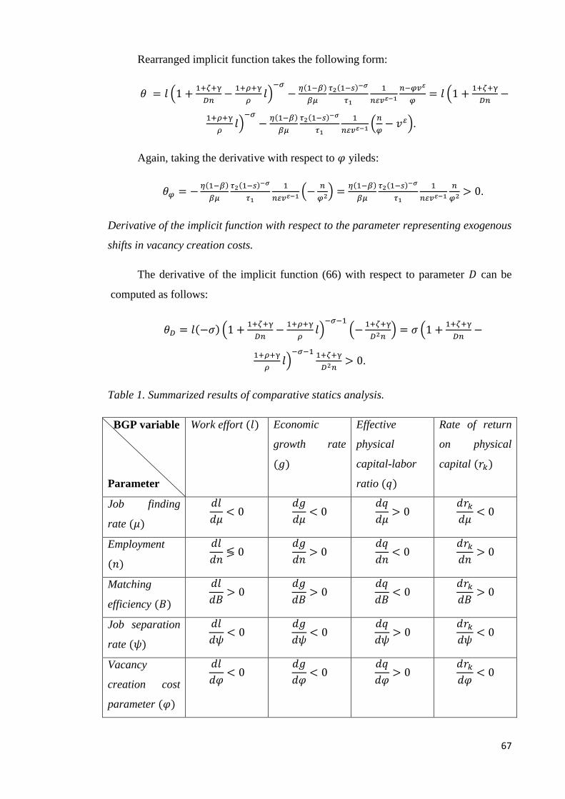
67
Rearranged implicit function takes the following form:
(
)
(
)
(
).
Again, taking the derivative with respect to yileds:
(
)
.
Derivative of the implicit function with respect to the parameter representing exogenous
shifts in vacancy creation costs.
The derivative of the implicit function (66) with respect to parameter can be
computed as follows:
(
)
(
) (
)
.
Table 1. Summarized results of comparative statics analysis.
BGP variable
Parameter
Work effort Economic
growth rate
Effective
physical
capital-labor
ratio
Rate of return
on physical
capital
Job finding
rate
Employment
Matching
efficiency
Job separation
rate
Vacancy
creation cost
parameter

68
Maximum rate
of endogenous
human capital
accumulation
in the
short run,
in the
long run
in the
short run,
in the
long run
in the
short run,
in the
long run
Exogenous shift
in human
capital
accumulation
Spillover effect
from physical
capital .

69
Appendix D.
Derivation of equation (69).
Using the assumption that in (68) results in:
,
from which it follows that
. (69)
Derivation of equation (71).
As it was stated before, profit per vacancy is expressed in the following way:
.
Let me consider the parts of this equation on by one. Firstly, output per worker
can be rearranged to get:
[( ) ]
[
( ) ]
( )
( )
.
Then, the cost of physical capital per filled vacancy takes the form of:
[
( ) ]
[
( ) ]
( )
( )
.
Plugging all these results into the expression for profit per vacancy I get:
( )
( )
( )
[ ( )
] ,
which in the end gives the desired expression (71).
Derivation of equation (73).
Using
in (72) and equating it to (69) gives:
,
which is then rearranged to get (73):

70
. (73)
Derivation of equation (76).
Plugging (74) and (75) into (70) and using free-entry condition allows obtaining
the second expression for profit per filled vacancy (76):
.
Derivation of equation (77).
Equating (71) and (76) gives:
[ ( )
]
,
,
,
which, finally, results in (77):
[
] . (77)
Now it is time to make (77) easier for analysis and comparison. Firstly, let me
consider the part
( ) .
From the very first rearranged FOC (19) it can be inferred that:
( ) ( )
.
Therefore,
( ).
Consequently,
( )
.
From (17),
.

71
It was explained before that , thus
.
By applying functional forms to the latter, one obtains:
.
This, finally, can be plugged into the expression for the wage instead of
:
[
] .
Rearranging this gives:
[ {
}] , (78)
where
.