Lab 4 GMT and Projection with ArcGISgeoscience.unlv.edu/pub/snelson/GIS/Lab4_Topos_Projections.pdf · Lab 4: Making Maps with ... NevadaCounties, UTM Zone 11 NAD83, meters. NevadaCounties_dd,

GEY 430/630 – GIS – Theory and Application

Projections: 1

Lab 4: Making Maps with GMT and Projecting Geographic Data in ArcGIS

Purpose: Provide you with alternative ways to make images and to introduce you to

projection among coordinate systems. To Do: Create a topographic map in GMT using various projections. Project shapefiles

among coordinate systems in ArcGIS. To Turn In: (1.) A map of three different views of projected data (remember to add scale bar,

title, name, north arrow, legend, etc., for each view), (2.) the area of Nye County after several different reprojections and a list of the coordinates for a point in four different coordinate systems, and a (3.) map of reprojected roads data.

Data Used: topo_grid.gmt color.gmt NevadaCounties, UTM Zone 11 NAD83, meters. NevadaCounties_dd, geographic coordinates, decimal degrees roads, State Plane, NAD27, Nevada East Zone Extensions Required: none Data Source: Part I: /home/GIS/GIS/

Part II: S:\GEY430_630_Spr04\projex

The Earth's surface is curved in two directions. When you flatten this compound curved surface to plot a map, you introduce distortion. Different map projections introduce different types of distortion, and organizations choose the projection which limits distortions to levels they can accept. You cannot mix different map projections in an analysis, that is, all coverages, shapefiles, or data files must be in the same map projection. Thus, you often have to project data from one coordinate system to another prior to starting your analysis.


Projections: 2

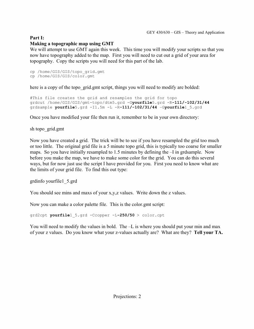
Part I: Making a topographic map using GMT We will attempt to use GMT again this week. This time you will modify your scripts so that you now have topography added to the map. First you will need to cut out a grid of your area for topography. Copy the scripts you will need for this part of the lab. cp /home/GIS/GIS/topo_grid.gmt cp /home/GIS/GIS/color.gmt here is a copy of the topo_grid.gmt script, things you will need to modify are bolded: #This file creates the grid and resamples the grid for topo grdcut /home/GIS/GIS/gmt-topo/dtm5.grd -Gyourfile5.grd -R-111/-102/31/44 grdsample yourfile5.grd -I1.5m -L -R-111/-102/31/44 –Gyourfile1_5.grd Once you have modified your file then run it, remember to be in your own directory: sh topo_grid.gmt Now you have created a grid. The trick will be to see if you have resampled the grid too much or too little. The original grid file is a 5 minute topo grid, this is typically too coarse for smaller maps. So you have initially resampled to 1.5 minutes by defining the –I in grdsample. Now before you make the map, we have to make some color for the grid. You can do this several ways, but for now just use the script I have provided for you. First you need to know what are the limits of your grid file. To find this out type: grdinfo yourfile1_5.grd You should see mins and maxs of your x,y,z values. Write down the z values. Now you can make a color palette file. This is the color.gmt script: grd2cpt yourfile1_5.grd -Ccopper -L-250/50 > color.cpt You will need to modify the values in bold. The –L is where you should put your min and max of your z values. Do you know what your z-values actually are? What are they? Tell your TA.


Projections: 3

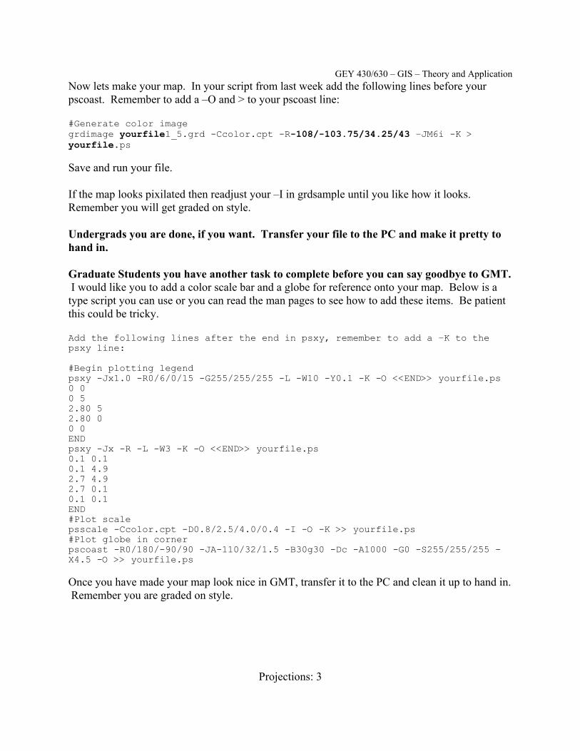
Now lets make your map. In your script from last week add the following lines before your pscoast. Remember to add a –O and > to your pscoast line: #Generate color image grdimage yourfile1_5.grd -Ccolor.cpt -R-108/-103.75/34.25/43 –JM6i -K > yourfile.ps Save and run your file. If the map looks pixilated then readjust your –I in grdsample until you like how it looks. Remember you will get graded on style. Undergrads you are done, if you want. Transfer your file to the PC and make it pretty to hand in. Graduate Students you have another task to complete before you can say goodbye to GMT. I would like you to add a color scale bar and a globe for reference onto your map. Below is a type script you can use or you can read the man pages to see how to add these items. Be patient this could be tricky. Add the following lines after the end in psxy, remember to add a –K to the psxy line: #Begin plotting legend psxy -Jx1.0 -R0/6/0/15 -G255/255/255 -L -W10 -Y0.1 -K -O <<END>> yourfile.ps 0 0 0 5 2.80 5 2.80 0 0 0 END psxy -Jx -R -L -W3 -K -O <<END>> yourfile.ps 0.1 0.1 0.1 4.9 2.7 4.9 2.7 0.1 0.1 0.1 END #Plot scale psscale -Ccolor.cpt -D0.8/2.5/4.0/0.4 -I -O -K >> yourfile.ps #Plot globe in corner pscoast -R0/180/-90/90 -JA-110/32/1.5 -B30g30 -Dc -A1000 -G0 -S255/255/255 -X4.5 -O >> yourfile.ps Once you have made your map look nice in GMT, transfer it to the PC and clean it up to hand in. Remember you are graded on style.


Projections: 4

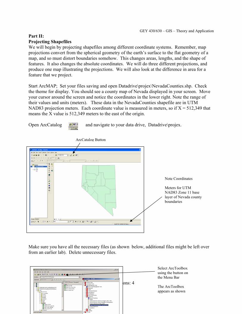
Part II: Projecting Shapefiles We will begin by projecting shapefiles among different coordinate systems. Remember, map projections convert from the spherical geometry of the earth’s surface to the flat geometry of a map, and so must distort boundaries somehow. This changes areas, lengths, and the shape of features. It also changes the absolute coordinates. We will do three different projections, and produce one map illustrating the projections. We will also look at the difference in area for a feature that we project. Start ArcMAP; Set your files saving and open Datadrive\projex\NevadaCounties.shp. Check the theme for display. You should see a county map of Nevada displayed in your screen. Move your cursor around the screen and notice the coordinates in the lower right. Note the range of their values and units (meters). These data in the NevadaCounties shapefile are in UTM NAD83 projection meters. Each coordinate value is measured in meters, so if X = 512,349 that means the X value is 512,349 meters to the east of the origin. Open ArcCatalog and navigate to your data drive, Datadrive\projex. Make sure you have all the necessary files (as shown below, additional files might be left over from an earlier lab). Delete unnecessary files.

Note Coordinates Meters for UTM NAD83 Zone 11 base layer of Nevada county boundaries

ArcCatalog Button

Select ArcToolbox using the button on the Menu Bar The ArcToolbox appears as shown


Projections: 5

In Arc Toolbox click on Data Management Tools, Projections, Select the Project Wizard (shapefiles, geodatabase) The Project Wizard steps you through the process of reprojecting a data layer to another geographic or projected layer. There are several steps and options to select. In ArcToolbox - The basic process is:

• Select a starting layer (the one you wish to reproject; don’t worry you original is not altered) • Select a place to put the new (reprojected) layer. • Select the reprojection parameters (they might require both projection and geographic

parameters). These parameters can be loaded from another layer already in you new projection or can create a new set of parameters.

• Apply the reprojection parameters • Decide on the transformation process (often you take the default) • Complete the process

Useful background note:ArcGIS layers, shapefiles, coverages, and grids all require projection information in a special file. For example, if your layer is named NevadaCounties.shp then the projection information is stored in a file called NevadaCounties.prj. This Wizard helps you create and maintain this essential projection information file. This document will step you through the screens the first time. You will have to use these steps at least six (6) more times in this lab. For later steps refer back to this process flow.

Start the Project Wizard Browse to the layer you wish to reproject For the 1st step use NevadaCounties.shp located in Datadrive\projex Then select Next


Projections: 6


Projections: 7

Now navigate to where you want the new (reprojected) file to be. Name the file; you don’t need to type in the .shp last name. For this 1st step name the new file NevadaCounties_albers Press Save and then Next

Then push Select Coordinate System

Now you must Select or Import parameters for reprojection. Often it is easier importing from another layer that has the projection you want. For this 1st step push the Select button


Projections: 8

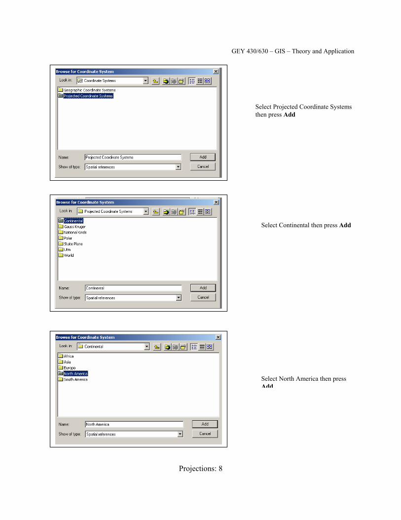
Select Projected Coordinate Systems then press Add

Select Continental then press Add

Select North America then press Add


Projections: 9

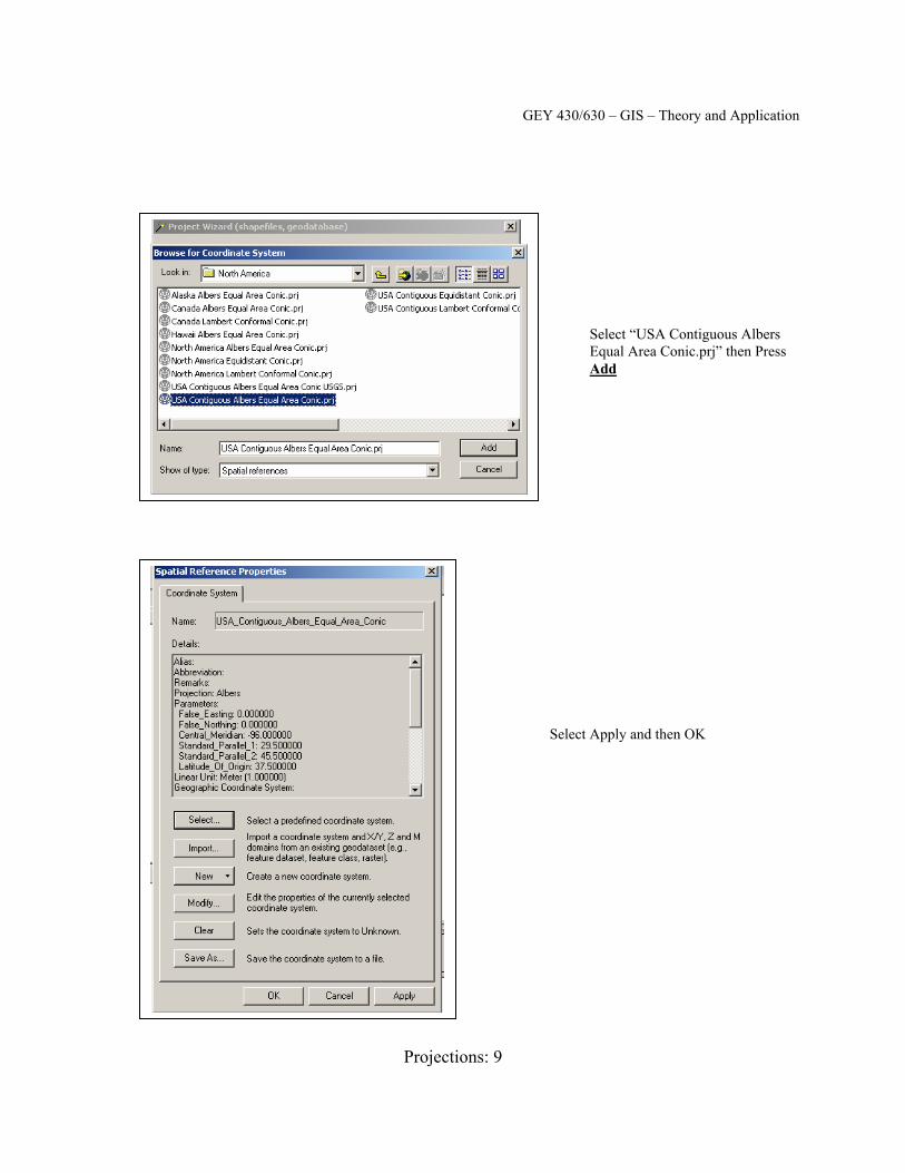
Select “USA Contiguous Albers Equal Area Conic.prj” then Press Add

Select Apply and then OK


Projections: 10

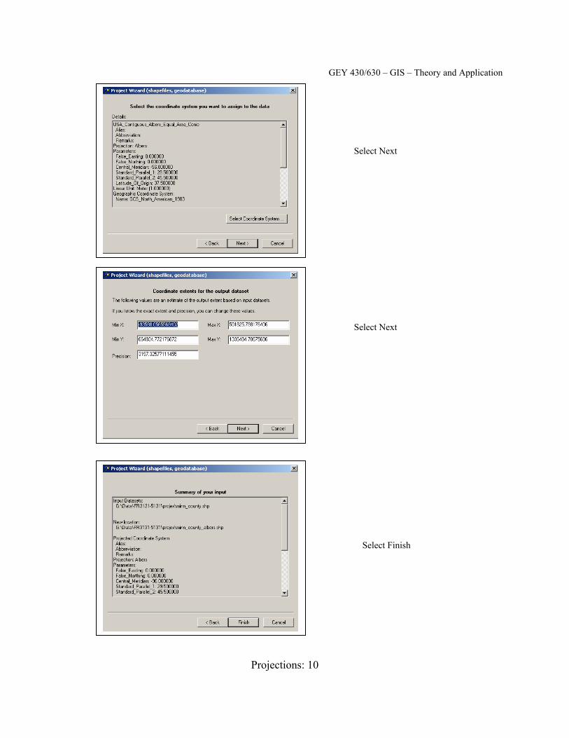
Select Next

Select Next

Select Finish


Projections: 11

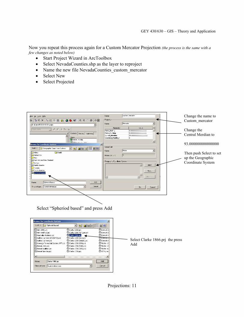
Now you repeat this process again for a Custom Mercator Projection (the process is the same with a few changes as noted below)

• Start Project Wizard in ArcToolbox • Select NevadaCounties.shp as the layer to reproject • Name the new file NevadaCounties_custom_mercator • Select New • Select Projected

Change the name to Custom_mercator Change the Central Merdian to 93.000000000000000 Then push Select to set up the Geographic Coordinate System

Select “Spheriod based” and press Add

Select Clarke 1866.prj the press Add


Projections: 12

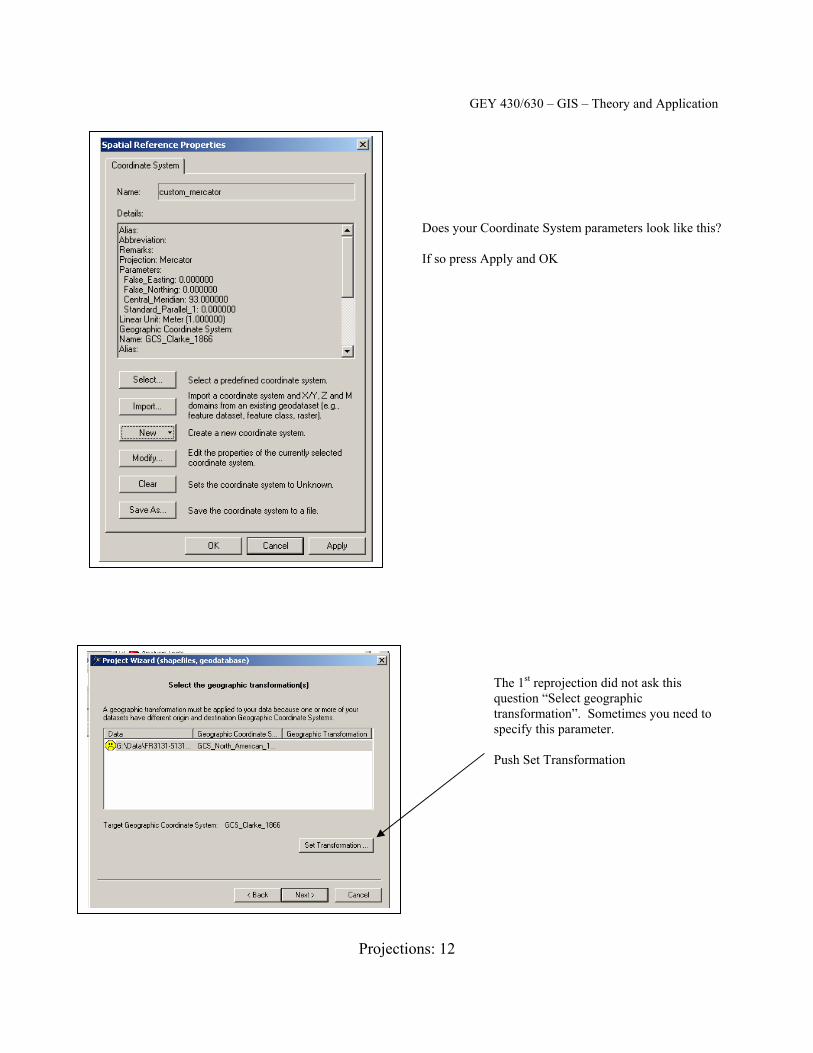
Does your Coordinate System parameters look like this? If so press Apply and OK

The 1st reprojection did not ask this question “Select geographic transformation”. Sometimes you need to specify this parameter. Push Set Transformation


Projections: 13

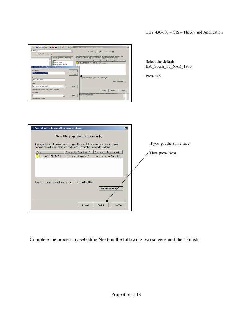
Complete the process by selecting Next on the following two screens and then Finish.

Select the default Bab_South_To_NAD_1983 Press OK

If you got the smile face Then press Next


Projections: 14

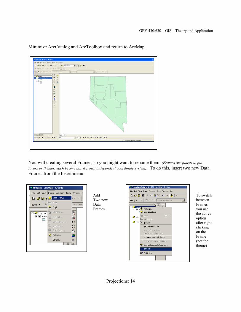
Minimize ArcCatalog and ArcToolbox and return to ArcMap. You will creating several Frames, so you might want to rename them (Frames are places to put layers or themes, each Frame has it’s own independent coordinate system). To do this, insert two new Data Frames from the Insert menu.

Add Two new Data Frames

To switch between Frames you use the active option after right clicking on the Frame (not the theme)


Projections: 15

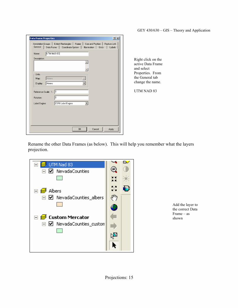
Rename the other Data Frames (as below). This will help you remember what the layers projection.

Right click on the active Data Frame and select Properties. From the General tab change the name. UTM NAD 83

Add the layer to the correct Data Frame – as shown


Projections: 16

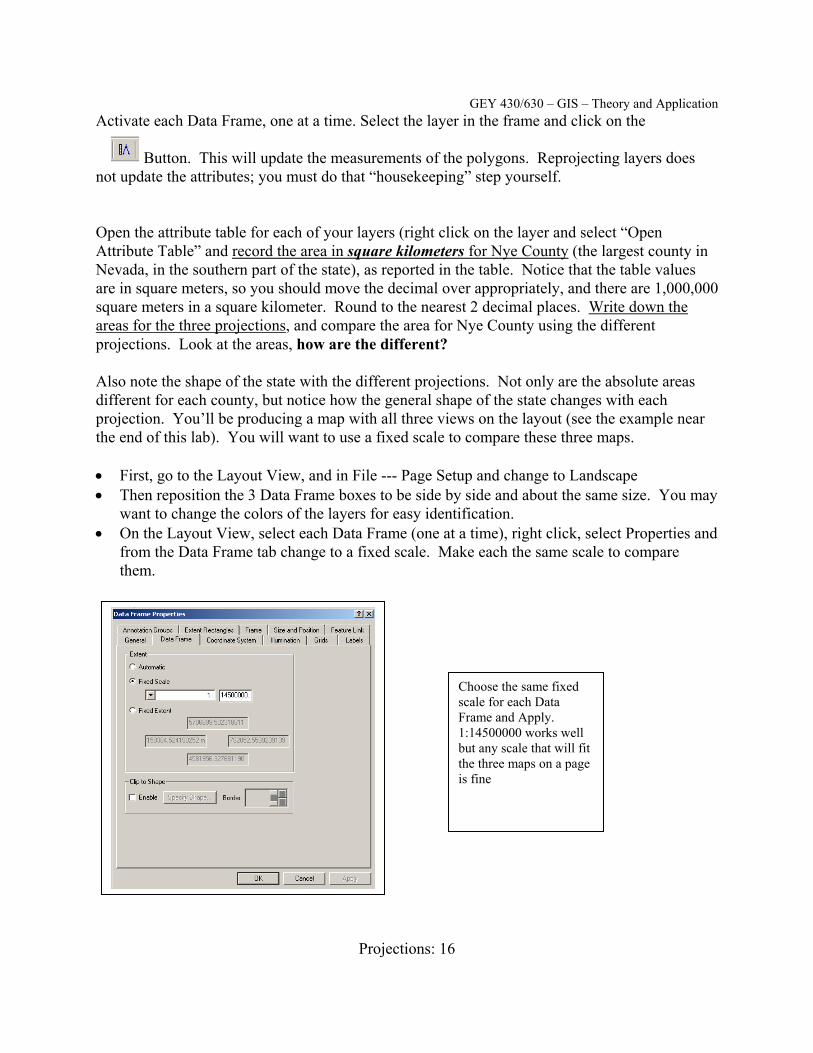
Activate each Data Frame, one at a time. Select the layer in the frame and click on the Button. This will update the measurements of the polygons. Reprojecting layers does not update the attributes; you must do that “housekeeping” step yourself. Open the attribute table for each of your layers (right click on the layer and select “Open Attribute Table” and record the area in square kilometers for Nye County (the largest county in Nevada, in the southern part of the state), as reported in the table. Notice that the table values are in square meters, so you should move the decimal over appropriately, and there are 1,000,000 square meters in a square kilometer. Round to the nearest 2 decimal places. Write down the areas for the three projections, and compare the area for Nye County using the different projections. Look at the areas, how are the different? Also note the shape of the state with the different projections. Not only are the absolute areas different for each county, but notice how the general shape of the state changes with each projection. You’ll be producing a map with all three views on the layout (see the example near the end of this lab). You will want to use a fixed scale to compare these three maps. • First, go to the Layout View, and in File --- Page Setup and change to Landscape • Then reposition the 3 Data Frame boxes to be side by side and about the same size. You may

want to change the colors of the layers for easy identification. • On the Layout View, select each Data Frame (one at a time), right click, select Properties and

from the Data Frame tab change to a fixed scale. Make each the same scale to compare them.

Choose the same fixed scale for each Data Frame and Apply. 1:14500000 works well but any scale that will fit the three maps on a page is fine


Projections: 17

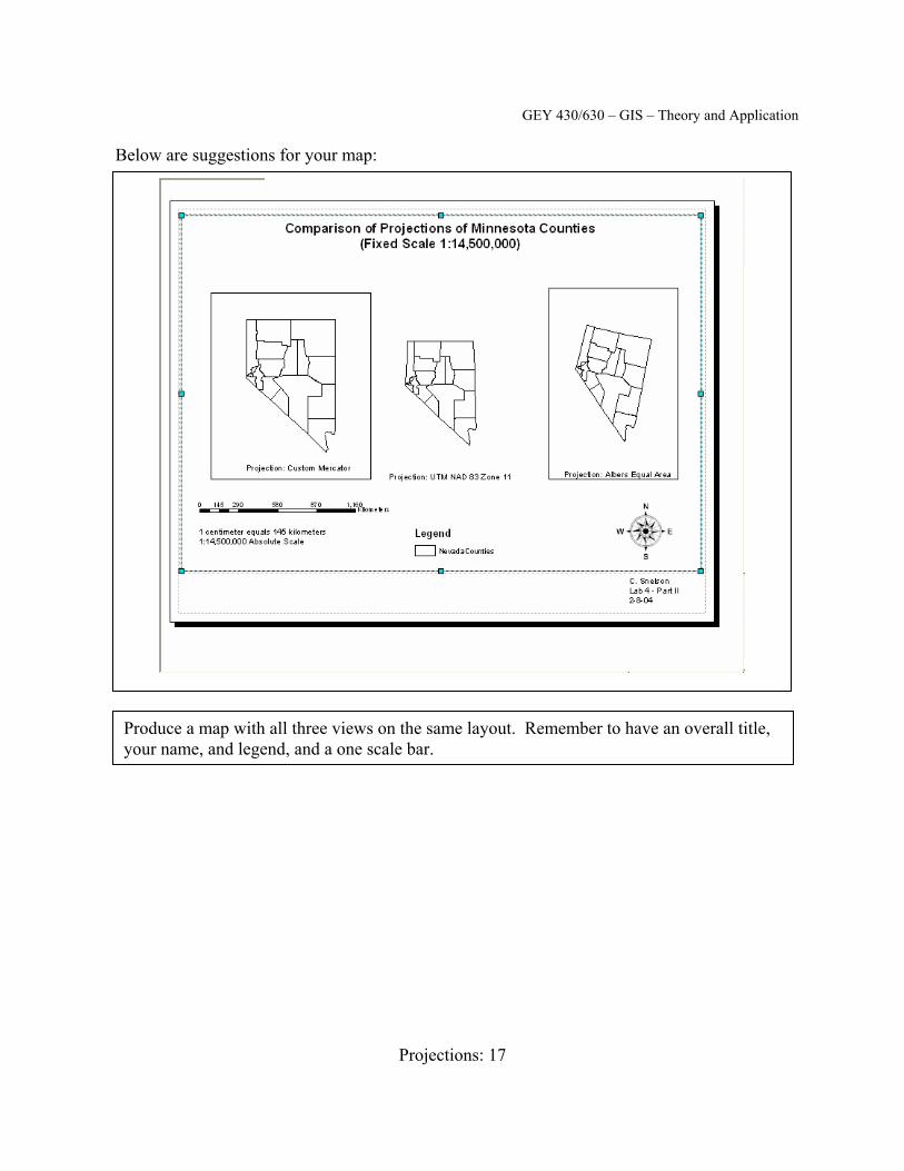
Produce a map with all three views on the same layout. Remember to have an overall title, your name, and legend, and a one scale bar.

Below are suggestions for your map:


Projections: 18

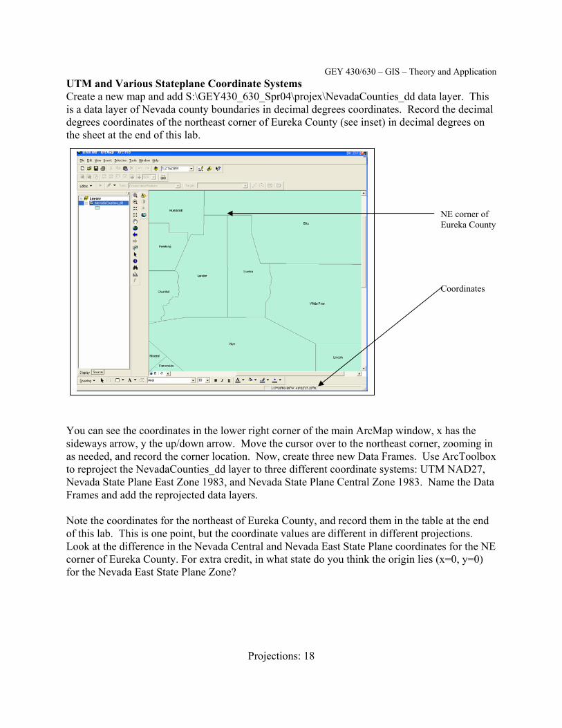
UTM and Various Stateplane Coordinate Systems Create a new map and add S:\GEY430_630_Spr04\projex\NevadaCounties_dd data layer. This is a data layer of Nevada county boundaries in decimal degrees coordinates. Record the decimal degrees coordinates of the northeast corner of Eureka County (see inset) in decimal degrees on the sheet at the end of this lab. You can see the coordinates in the lower right corner of the main ArcMap window, x has the sideways arrow, y the up/down arrow. Move the cursor over to the northeast corner, zooming in as needed, and record the corner location. Now, create three new Data Frames. Use ArcToolbox to reproject the NevadaCounties_dd layer to three different coordinate systems: UTM NAD27, Nevada State Plane East Zone 1983, and Nevada State Plane Central Zone 1983. Name the Data Frames and add the reprojected data layers. Note the coordinates for the northeast of Eureka County, and record them in the table at the end of this lab. This is one point, but the coordinate values are different in different projections. Look at the difference in the Nevada Central and Nevada East State Plane coordinates for the NE corner of Eureka County. For extra credit, in what state do you think the origin lies (x=0, y=0) for the Nevada East State Plane Zone?

NE corner of Eureka County Coordinates


Projections: 19

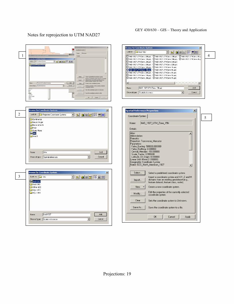
Notes for reprojection to UTM NAD27

1

2

3

4

5


Projections: 20

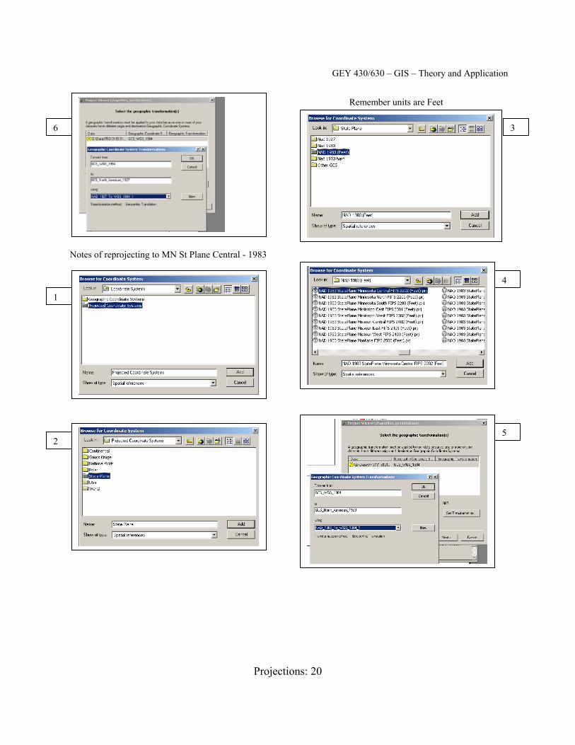
Notes of reprojecting to MN St Plane Central - 1983

1

2

6 3

4

5

Remember units are Feet


Projections: 21

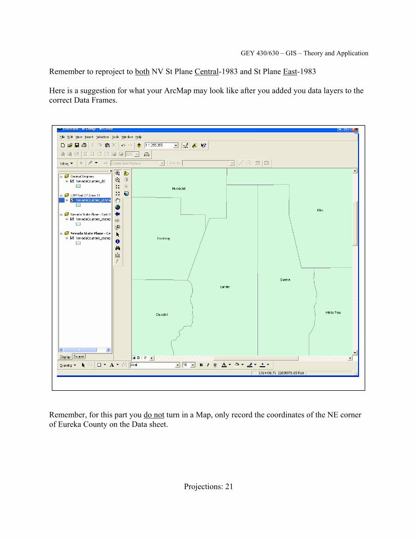
Remember to reproject to both NV St Plane Central-1983 and St Plane East-1983 Here is a suggestion for what your ArcMap may look like after you added you data layers to the correct Data Frames. Remember, for this part you do not turn in a Map, only record the coordinates of the NE corner of Eureka County on the Data sheet.


Projections: 22

Now we will change the projection for a data layer. You often have to do this when data are developed or delivered in one map projection, and you are working with other data on a project in another map projection. In our example we will convert data from state plane coordinates to UTM coordinates. Open a new ArcMap and display the following two files in the same Data Frame S:\GEY430_630_Spr04\projex\NevadaCounties.shp NV Counties S:\GEY430_630_Spr04\projex\roads.shp Las Vegas Roads Click on the zoom to full extent button, and notice the relative location of the data contained in the two layers. roads contains roads of Las Vegas. The data are wrongly displaced relative to each other because different units are used, different projection shapes and origins, and so the data are projected to a different set of coordinates. This illustrates why you need to be careful in not mixing data with different projections. Now to change the projection for the data. • Use ArcToolbox to reproject roads to UTM NAD83. • Add the new reprojected layer to the Data Frame with NevadaCounties • Notice how the two road layers are shifted from each other. • Remove the old roads layer. Rearrange/recolor the data layers so you can see both the county and roads. Notice the new, correct locations for these roads.


Projections: 23

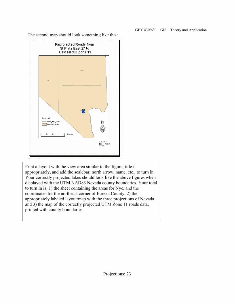
Print a layout with the view area similar to the figure, title it appropriately, and add the scalebar, north arrow, name, etc., to turn in. Your correctly projected lakes should look like the above figures when displayed with the UTM NAD83 Nevada county boundaries. Your total to turn in is: 1) the sheet containing the areas for Nye, and the coordinates for the northeast corner of Eureka County. 2) the appropriately labeled layout/map with the three projections of Nevada, and 3) the map of the correctly projected UTM Zone 11 roads data, printed with county boundaries.

The second map should look something like this:


Projections: 24

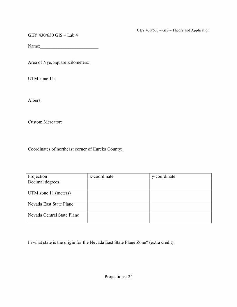
GEY 430/630 GIS – Lab 4 Name:_________________________ Area of Nye, Square Kilometers: UTM zone 11: Albers: Custom Mercator: Coordinates of northeast corner of Eureka County: Projection x-coordinate y-coordinate Decimal degrees

UTM zone 11 (meters)

Nevada East State Plane

Nevada Central State Plane

In what state is the origin for the Nevada East State Plane Zone? (extra credit):


Projections: 25

GEY 430/630 GIS – Lab 4 Name:_________________________ Suggestions for Improvement: Projection Lab Please help me improve this lab. As incentive, any improvements incorporated (or major errors removed) will gain you a point on your final grade total. What didn't work in this lab, and how would you fix it? What was the best part of this lab exercise?

Documents

Lab 4 GMT and Projection with ArcGISgeoscience.unlv.edu/pub/snelson/GIS/Lab4_Topos_Projections.pdf · Lab 4: Making Maps with ... NevadaCounties, UTM Zone 11 NAD83, meters. NevadaCounties_dd,