Lab 3 – Counting Statistics - University of Michiganianrit/Lab3short.pdf · Rittersdorf Lab 3 - Counting Statistics data than the Gaussian distribution. To better investigate this,

Lab 3 – Counting Statistics

Ian RittersdorfNuclear Engineering & Radiological Sciences

[email protected]

February 22, 2007

Rittersdorf Lab 3 - Counting Statistics

1 Abstract

In this lab we took many samples of counts. For one experiment we took 25 samples of countson the order of 104. For another experiment we took 1000 samples of very small counts. Weapplied tests to see if a Gaussian or Poisson distribution modelled either of these sets ofmeasurements well. Theory predicts that for very large counts, a Gaussian distribution willaccurately model the data. Theory also predicts that for small counts that the Poissondistribution will accurately model that data. In the lab, we found this to be true. The fewsamples of large counts resembled a Gaussian distribution and the large sample number ofthe small counts resembled a Poisson distribution. In all, the experimental results matchedup with theory, literature, and calculations.

2 Introduction & Objectives

So far, in lab, we have already familiarized ourselves with the equipment that we will be thebasis of what we are using for the rest of the semester. The next step in becoming brilliant,young scientists is to learn what to do with the data once it is collected. The purpose of thislab is to get accustomed to the statistical analysis of laboratory measurements. The actual inlab time was relatively short as all that we were doing was collecting sets of counts. The realbulk of this lab is the analysis that is done outside of the laboratory to build our intuitionof counting statistics. It is quite imperative in the laboratory to understand how precise ameasurement is. Taking more measurements increases the accuracy of a measurement, butit is important to understand to what extent the precision of the measurement is increased.It is the objective of this lab to explore just that.

3 Experiment Part 5

3.1 Setup & Procedure

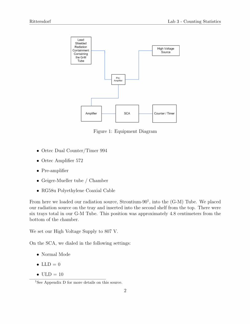
To setup our experiment, we set up our equipment as follows:First, we connected the pre-amplifier to a high voltage power supply and a Geiger-Mueller(G-M) Tube. From there, the pre-amplifier output is connected to an amplifier, then to anSCA, and finally to a counter/timer. As we did this, we would plug the outputs into ouroscilloscope to make sure that we were getting proper output. We used coaxial cable to makeall connections.

The specific equipment models that we used are:

• Hewlett-Packard 54610 B Oscilloscope

• Tennelec TC 952A High Voltage Supply

1


Figure 1: Equipment Diagram

• Ortec Dual Counter/Timer 994

• Ortec Amplifier 572

• Pre-amplifier

• Geiger-Mueller tube / Chamber

• RG58u Polyethylene Coaxial Cable

From here we loaded our radiation source, Strontium-901, into the (G-M) Tube. We placedour radiation source on the tray and inserted into the second shelf from the top. There weresix trays total in our G-M Tube. This position was approximately 4.8 centimeters from thebottom of the chamber.

We set our High Voltage Supply to 807 V.

On the SCA, we dialed in the following settings:

• Normal Mode

• LLD = 0

• ULD = 10

1See Appendix D for more details on this source.

2


• Pos Out

On the Amplifier, we dialed in the following settings:

• Unipolar

• Gain = 7.12

• Coarse Gain = 100

• Shaping time = 2 µs

• Negative Polarity

Maintaining of these settings, we varied the counter time and experimented with the counteruntil it was returning values that looked like they were averaging around 30 counts per tim-ing interval.

The time interval on our Counter/Timer was set to 0.05 s. After having all of this set up,our counts were giving us an average value of 30. We then recorded a set of 25 of thesecounts.

3.2 Results & Analysis

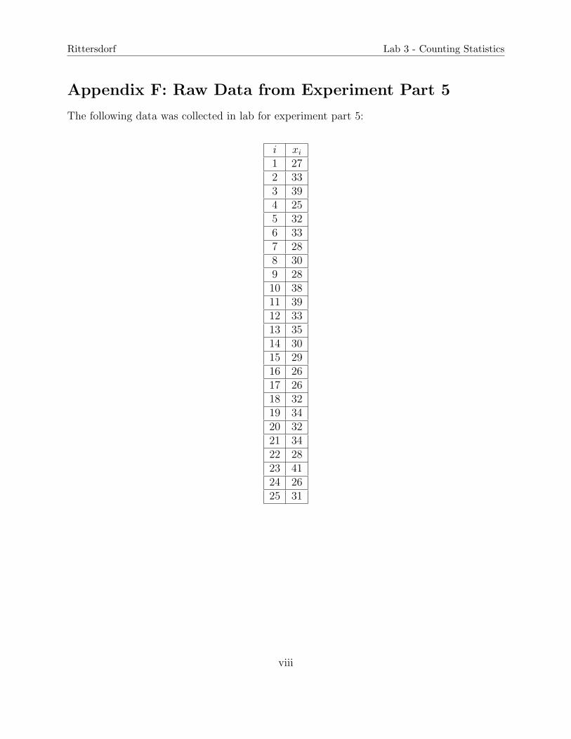
From the data that we calculated in the lab2, we wished to calculate the experimental mean:

x̄e =1

25

∑i

xi (1)

and the sample variance:

s2 =1

24

∑i

(xi − x̄e)2 (2)

Using these formulas and the data collected in lab, the following values were calculated:

x̄e = 31.56s2 = 19.9233

s =√

s2 = 4.46355

2See Appendix F to view the raw data collected in lab.

3


If this is a true Poisson distribution, we expect that the standard deviation for one typicalmeasurement should be

σi =√

xi∼=

√x̄e (3)

since the experimental mean is approximately the same as any typical value. Therefore, ifthe data truly fits the Poisson model, then the value of s that we calculated earlier shouldbe approximately the same as the σx̄e that we calculate.

Using Eq. (3), we calculate√

x̄e = 5.618. When we compare this to the experimentallymeasured value of s = 4.46, we see that they are different. The error between them is

[5.618− 4.46

5.618

]· 100% = 20.61% Error

This is a reasonable amount of error. It is safe to say that the data from these 25 sampleshas a reasonable fit to the Poisson distribution because the relation that s ' σx̄e is satisfiedwithin reason.The significance of σ here is that it is the standard deviation from the mean. It tells thataverage distance away from the mean is σ. 68.3% of the data lies within a distance of σ fromthe mean if you have a true Gaussian distribution.

χ2 is just another parameter of the experimental data distribution and is defined as

χ2 ≡ 1

x̄e

N∑i=1

(xi − x̄e)2 (4)

and is related to the sample variance by

χ2 =(N − 1)s2

x̄e

(5)

The degree to which χ2 deviates from N – 1 corresponds directly to how far the Poissondistribution deviates from accurately modelling the data. In other words, the close that χ2

is to unity, the better the Poisson model fits the data.

Using our data we calculate the following χ2 value.

χ2 = 15.151

4


With this value for χ2, we look up the probability that a random sample from the truePoisson distribution would be larger than χ2. It is important to analyze the extreme ends ofthe probabilities. Very high probabilities are those that are greater than 0.98. They indicateabnormally small fluctuations in the data. Very low probabilities are those that are less than0.02. They indicate abnormally large fluctuations in the data. A probability of 0.50 wouldrepresent a perfect fit to the Poisson distribution for large data sets.

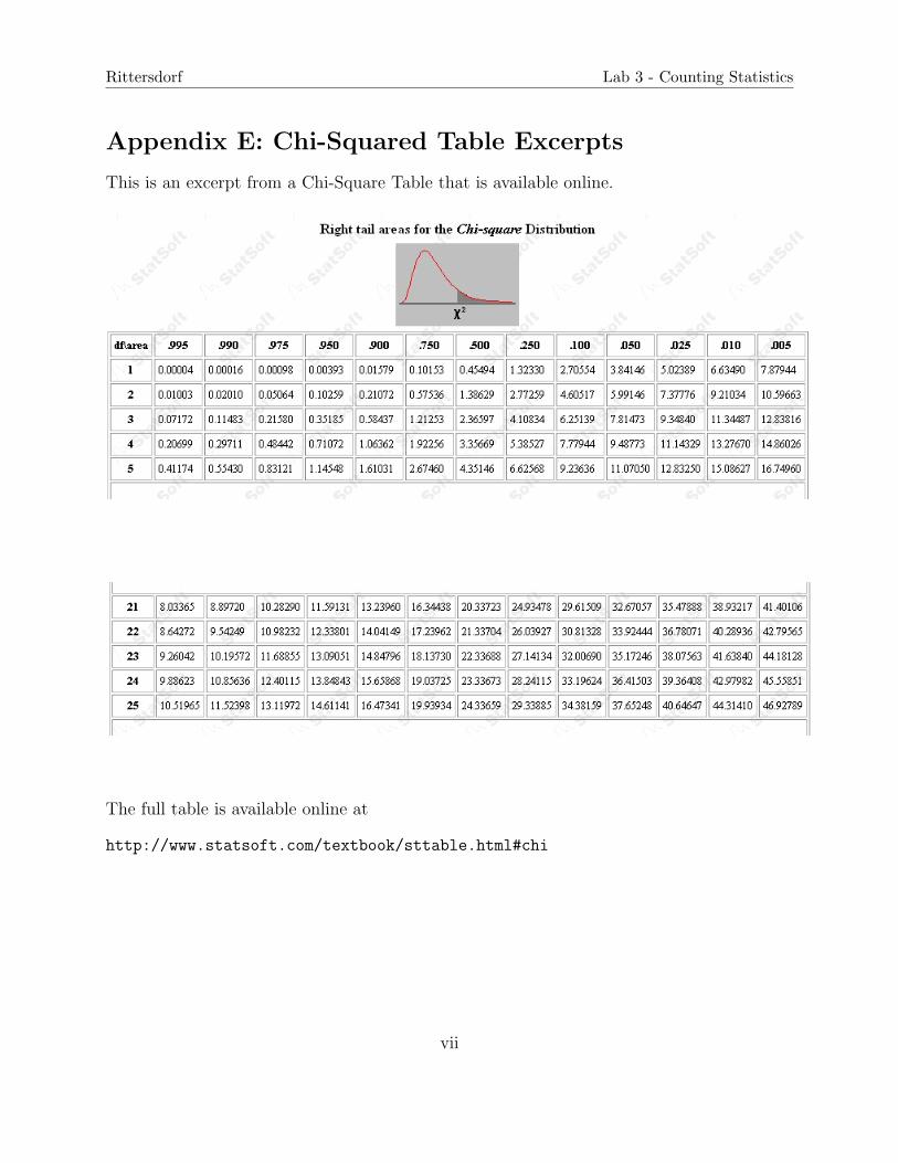
In order to look up a value of probability from the Chi-Squared table, you need two values:degrees of freedom and χ2. We have already calculated χ2. A system always has N – 1degrees of freedom, therefore our set of data has 24 degrees of freedom. A value for theprobability of our data being larger than χ2 is

p = 0.91627

This value is interpolated from a Chi-Squared distribution table.3

This probability of p = 0.91627 is neither extremely high or extremely low. Because of this,we can conclude that this set of numbers does not give rise to abnormal fluctuations. Thisvalue is starting to approach the higher end of the probabilities, however, and probably showssome small fluctuations. This lends itself to the fact that our data better fits a Gaussiandistribution because the Gaussian has a mean and a higher probabilities for values shiftedto the right of the Poisson model.

We know that for multiple samples

σx̄e =

√x̄e

N(6)

The expected uncertainty of the experimental mean is σx̄e =√

x̄e

N= 1.12. This uncertainty is

much smaller than any given σi. This is true because we have taken multiple measurementsand this reduces the statistical error. If you take the average of all of the σi’s and divide bythe improvement factor of 1√

N, you find that this exactly equals σx̄e . This is exactly what

we would expect.

4 Experiment Part 8

4.1 Setup & Procedure

The setup of this experiment was the same as the section 3.1 (see Figure 1) for details. Referto section 3.1 for specific settings.

3See Appendix E for the Chi-Squared table used to make this calculation.5


In order to collect an average of about 5 counts per timing interval, we maintained theprevious experiment’s settings and adjusted our counter time until we looked like we weregetting number around our desired average.

The time interval on our Counter/Timer was set to 0.01 s.

4.2 Results & Analysis

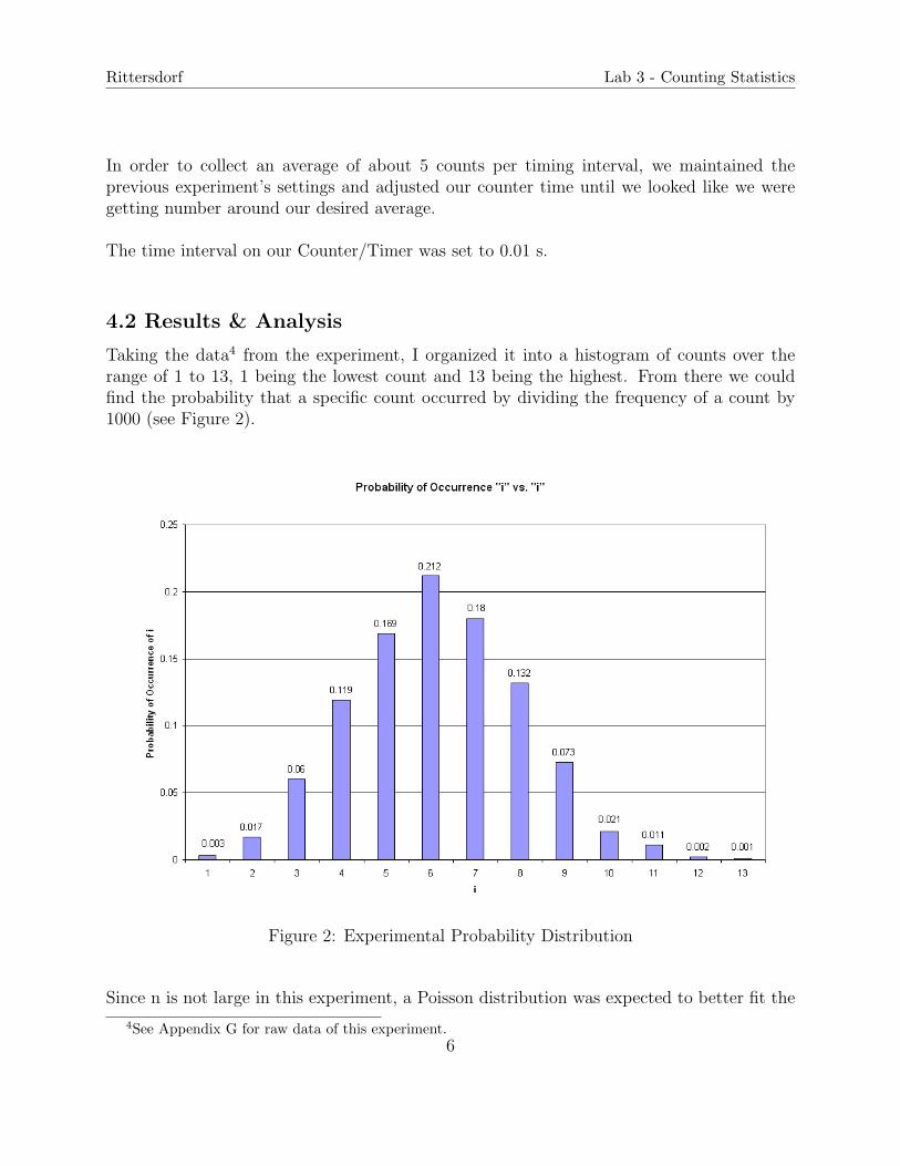
Taking the data4 from the experiment, I organized it into a histogram of counts over therange of 1 to 13, 1 being the lowest count and 13 being the highest. From there we couldfind the probability that a specific count occurred by dividing the frequency of a count by1000 (see Figure 2).

Figure 2: Experimental Probability Distribution

Since n is not large in this experiment, a Poisson distribution was expected to better fit the

4See Appendix G for raw data of this experiment.6


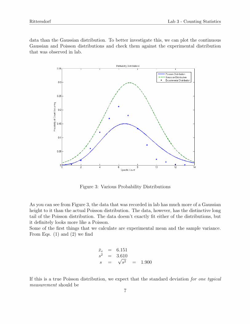
data than the Gaussian distribution. To better investigate this, we can plot the continuousGaussian and Poisson distributions and check them against the experimental distributionthat was observed in lab.

Figure 3: Various Probability Distributions

As you can see from Figure 3, the data that was recorded in lab has much more of a Gaussianheight to it than the actual Poisson distribution. The data, however, has the distinctive longtail of the Poisson distribution. The data doesn’t exactly fit either of the distributions, butit definitely looks more like a Poisson.Some of the first things that we calculate are experimental mean and the sample variance.From Eqs. (1) and (2) we find

x̄e = 6.151s2 = 3.610

s =√

s2 = 1.900

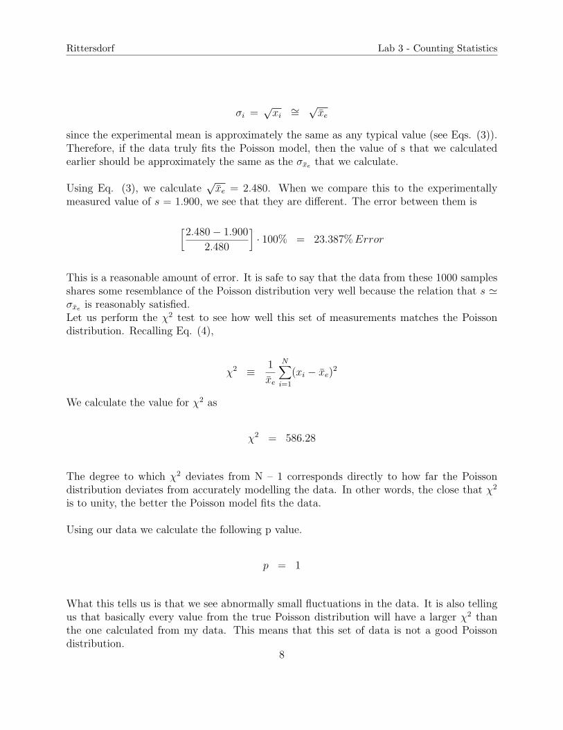
If this is a true Poisson distribution, we expect that the standard deviation for one typicalmeasurement should be

7


σi =√

xi∼=

√x̄e

since the experimental mean is approximately the same as any typical value (see Eqs. (3)).Therefore, if the data truly fits the Poisson model, then the value of s that we calculatedearlier should be approximately the same as the σx̄e that we calculate.

Using Eq. (3), we calculate√

x̄e = 2.480. When we compare this to the experimentallymeasured value of s = 1.900, we see that they are different. The error between them is

[2.480− 1.900

2.480

]· 100% = 23.387% Error

This is a reasonable amount of error. It is safe to say that the data from these 1000 samplesshares some resemblance of the Poisson distribution very well because the relation that s 'σx̄e is reasonably satisfied.Let us perform the χ2 test to see how well this set of measurements matches the Poissondistribution. Recalling Eq. (4),

χ2 ≡ 1

x̄e

N∑i=1

(xi − x̄e)2

We calculate the value for χ2 as

χ2 = 586.28

The degree to which χ2 deviates from N – 1 corresponds directly to how far the Poissondistribution deviates from accurately modelling the data. In other words, the close that χ2

is to unity, the better the Poisson model fits the data.

Using our data we calculate the following p value.

p = 1

What this tells us is that we see abnormally small fluctuations in the data. It is also tellingus that basically every value from the true Poisson distribution will have a larger χ2 thanthe one calculated from my data. This means that this set of data is not a good Poissondistribution.

8


5 Conclusions

Through the analysis of this lab, I witnessed firsthand the power of counting statistics. Boththe Poisson and the Gaussian distributions are useful and worthwhile tools for analyzingdistributions of data. Through the rigors of this lab, a deeper understanding of the finerpoints of counting statistics, such as χ2 values and standard deviations, was gained. Thisis important knowledge to have gained. In all of the labs in the future, I can now gathermore accurate data because I know to take more measurements to decrease error. I willalso report the error in future reports much more accurately. After completing this lab oncounting statistics, all of my future work as an engineer will be much higher in quality.

9


Appendices

Appendix A: Solutions to Select Ch. 3 Knoll Problems

Problem 6:

We know that we may apply σ =√

x only in certain circumstances. This rule does NOTapply directly to:

• Counting Rates

• Sums of Differences of Counts

• Averages of Independent Counts

• Any Derived Quantity

Therefore, we can rule out c, d, and e as solutions. Therefore, we can use σ =√

x for thefollowing:

a, b, and f

Problem 7:

time = 1 minS = 561 countsB = 410 countsNet count = S – B = 151 countsσnet =

√S + B = 31.2 counts

Thus,

151± 31.2

Problem 10:

We know that as a fraction for σ = 1√N

, where N is counts. We also know that N =ST, where S is the count rate and T is the time. Since we know that the count rate isconstant, we can say

σ21T1 = σ2

2T2

i


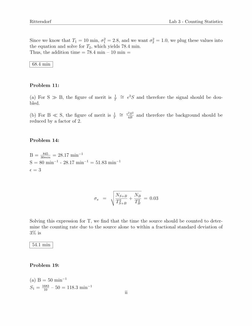
Since we know that T1 = 10 min, σ21 = 2.8, and we want σ2

2 = 1.0, we plug these values intothe equation and solve for T2, which yields 78.4 min.Thus, the addition time = 78.4 min – 10 min =

68.4 min

Problem 11:

(a) For S � B, the figure of merit is 1T∼= ε2S and therefore the signal should be dou-

bled.

(b) For B � S, the figure of merit is 1T∼= ε2S2

4Band therefore the background should be

reduced by a factor of 2.

Problem 14:

B = 84530min

= 28.17 min−1

S = 80 min−1 - 28.17 min−1 = 51.83 min−1

ε = 3

σs =

√√√√NS+B

T 2S+B

+NB

T 2B

= 0.03

Solving this expression for T, we find that the time the source should be counted to deter-mine the counting rate due to the source alone to within a fractional standard deviation of3% is

54.1 min

Problem 19:

(a) B = 50 min−1

S1 = 168310

– 50 = 118.3 min−1

ii


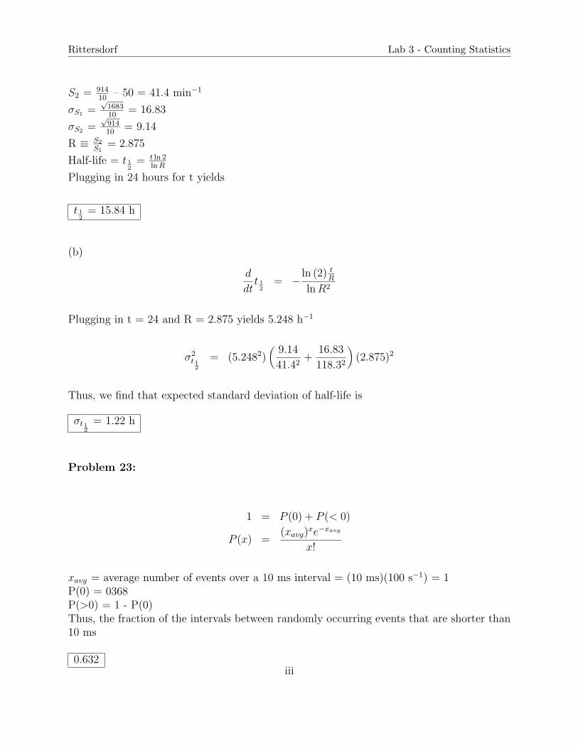
S2 = 91410

– 50 = 41.4 min−1

σS1 =√

168310

= 16.83

σS2 =√

91410

= 9.14

R ≡ S2

S1= 2.875

Half-life = t 12

= t ln 2ln R

Plugging in 24 hours for t yields

t 12

= 15.84 h

(b)

d

dtt 1

2= −

ln (2) tR

ln R2

Plugging in t = 24 and R = 2.875 yields 5.248 h−1

σ2t 12

= (5.2482)(

9.14

41.42+

16.83

118.32

)(2.875)2

Thus, we find that expected standard deviation of half-life is

σt 12

= 1.22 h

Problem 23:

1 = P (0) + P (< 0)

P (x) =(xavg)

xe−xavg

x!

xavg = average number of events over a 10 ms interval = (10 ms)(100 s−1) = 1P(0) = 0368P(>0) = 1 - P(0)Thus, the fraction of the intervals between randomly occurring events that are shorter than10 ms

0.632iii


Appendix B: Solution to Lab Problem 2

Single Count:

10982

Addition Counts:

10956 10719 1095310915 10843 1082610714 10769 11037

Important Equations:

σx =√

x

σr =σx

t

x̄ =

∑N

σx̄ =

√x̄

N

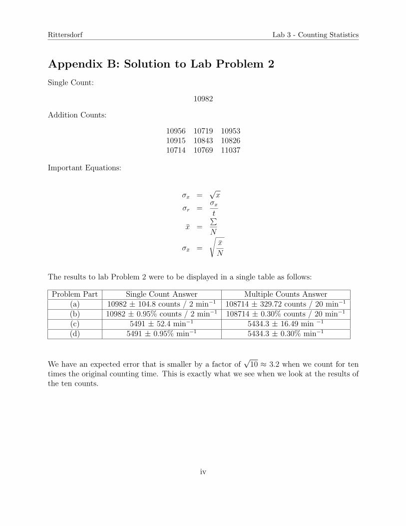
The results to lab Problem 2 were to be displayed in a single table as follows:

Problem Part Single Count Answer Multiple Counts Answer(a) 10982 ± 104.8 counts / 2 min−1 108714 ± 329.72 counts / 20 min−1

(b) 10982 ± 0.95% counts / 2 min−1 108714 ± 0.30% counts / 20 min−1

(c) 5491 ± 52.4 min−1 5434.3 ± 16.49 min −1

(d) 5491 ± 0.95% min−1 5434.3 ± 0.30% min−1

We have an expected error that is smaller by a factor of√

10 ≈ 3.2 when we count for tentimes the original counting time. This is exactly what we see when we look at the results ofthe ten counts.

iv


Appendix C: Solution to Lab Problem 3

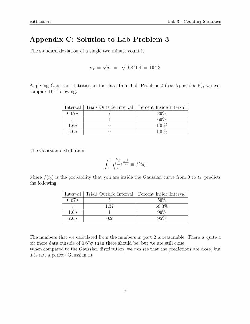
The standard deviation of a single two minute count is

σx̄ =√

x̄ =√

10871.4 = 104.3

Applying Gaussian statistics to the data from Lab Problem 2 (see Appendix B), we cancompute the following:

Interval Trials Outside Interval Percent Inside Interval0.67σ 7 30%

σ 4 60%1.6σ 0 100%2.0σ 0 100%

The Gaussian distribution

∫ t0

0

√2

πe−t2

2 ≡ f(t0)

where f(t0) is the probability that you are inside the Gaussian curve from 0 to t0, predictsthe following:

Interval Trials Outside Interval Percent Inside Interval0.67σ 5 50%

σ 1.37 68.3%1.6σ 1 90%2.0σ 0.2 95%

The numbers that we calculated from the numbers in part 2 is reasonable. There is quite abit more data outside of 0.67σ than there should be, but we are still close.When compared to the Gaussian distribution, we can see that the predictions are close, butit is not a perfect Gaussian fit.

v


Appendix D: Strontium 90 Data

Half-life = 28.79 yDecay mode(s) = β− (100%)Atomic Mass = 89.90773789 amuNuclear Mass = 89.8868919 amuBinding energy = 782.63 MeVBinding energy per nucleon = 8.6959 MeV/NucleonNatural abundance = –

Protons in nucleus = 38Neutrons in nucleus = 52Total nucleons = 90Number of electrons orbiting neutral atom = 38

Decay Chain:90Sr → 90Y → 90Zr

Both 90Sr and 90Y β− decay down to 90Zr, which is a stable isotope.

Production:90Sr is a product of nuclear fission. It is present in significant amounts in spent nuclear fueland radioactive waste from nuclear reactors. It is not that abundant in nature, so when itis needed, it is manufactured during the reprocessing of spent nuclear fuel.

Health Issues:When 90Sr gets into the human body, it usually deposits itself in the bones and bone marrow.When left there, 90Sr can cause bone cancer, leukiemia, and other cancers in nearby tissue.Urinalysis is used to dectect 90Sr in the human body.

Uses:90Sr has found its place in both medicine and industry. In the medical world, 90Sr is usedmost commonly used to treat bone cancer via radiotherapy. It is also used in industry as aradioactive source to gauge thicknesses. 90Sr generates a significant amount of heat in it’sdecay and is much cheaper than other heat producing isotopes which is why it found usein Russian / Soviet radioisotope thermoelectric generators. In addition to spacecraft, theSoviet Union constructed many unmanned lighthouses and navigation beacons powered byradioisotope thermoelectric generators.

Popular Culture:In a popular weekly British science fiction-oriented comic titled “2000 AD”, 90Sr showersmutate large portions of the world’s population, becoming the basis for the series.

vi


Appendix E: Chi-Squared Table Excerpts

This is an excerpt from a Chi-Square Table that is available online.

The full table is available online at

http://www.statsoft.com/textbook/sttable.html#chi

vii


Appendix F: Raw Data from Experiment Part 5

The following data was collected in lab for experiment part 5:

i xi

1 272 333 394 255 326 337 288 309 2810 3811 3912 3313 3514 3015 2916 2617 2618 3219 3420 3221 3422 2823 4124 2625 31

viii


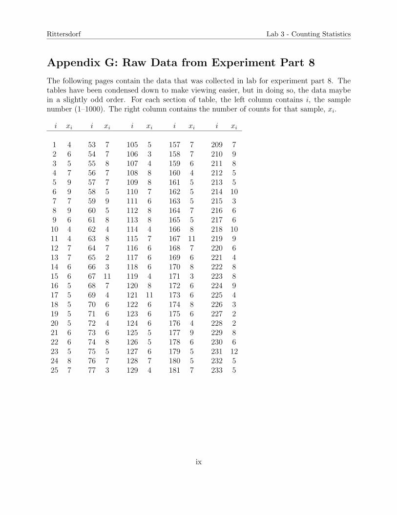
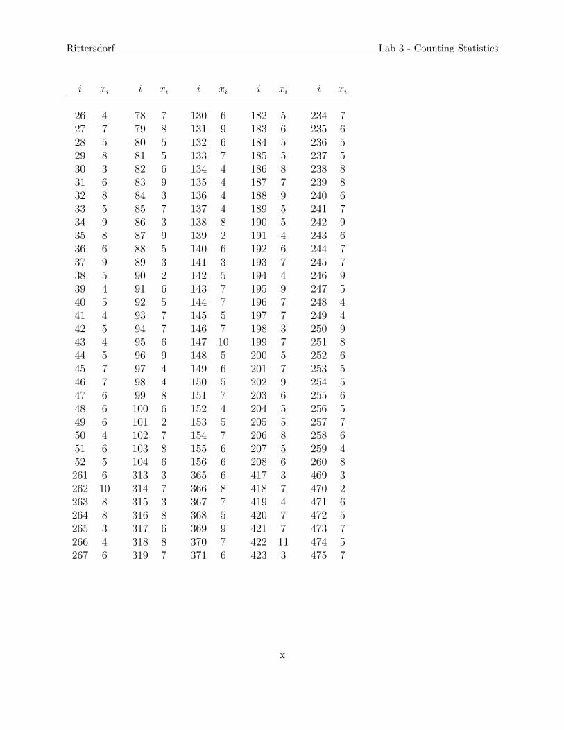
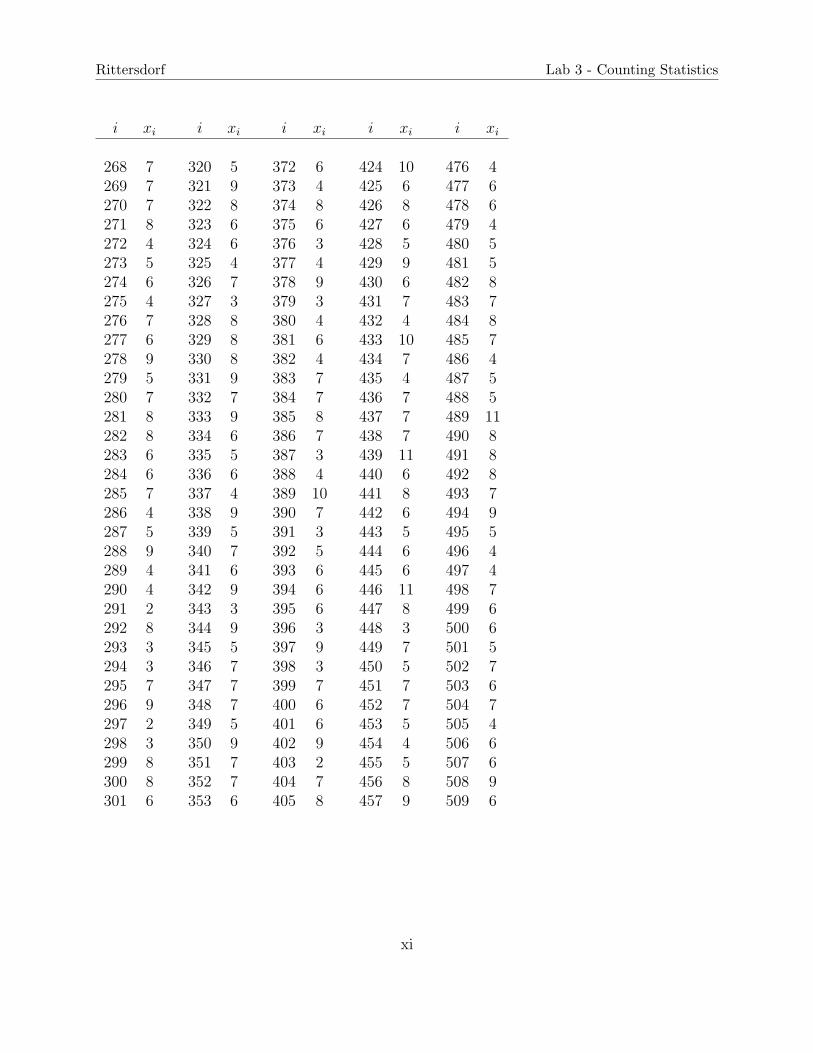
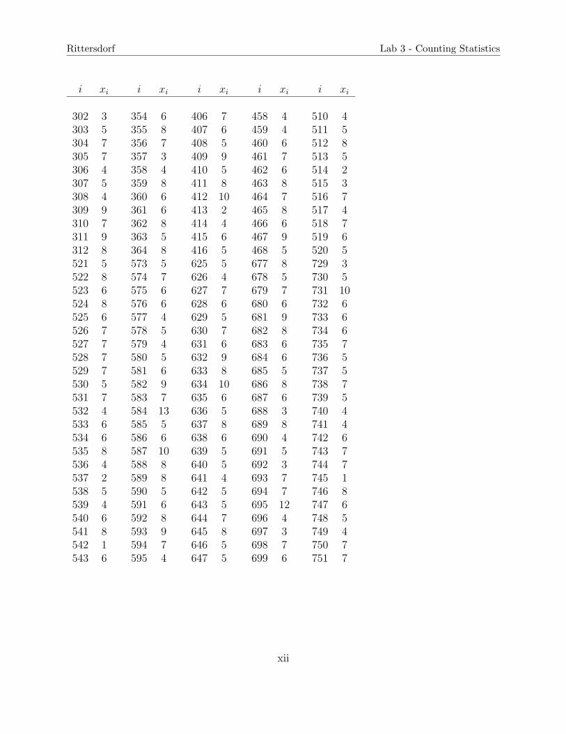
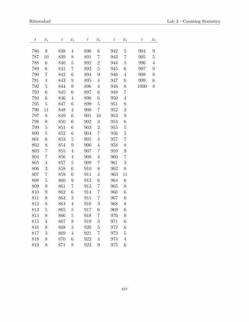
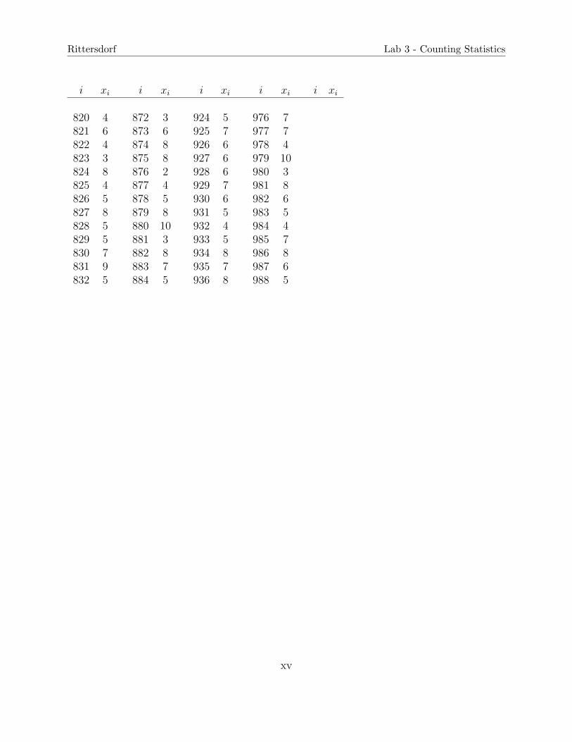
Appendix G: Raw Data from Experiment Part 8

The following pages contain the data that was collected in lab for experiment part 8. Thetables have been condensed down to make viewing easier, but in doing so, the data maybein a slightly odd order. For each section of table, the left column contains i, the samplenumber (1–1000). The right column contains the number of counts for that sample, xi.

i xi i xi i xi i xi i xi

1 4 53 7 105 5 157 7 209 72 6 54 7 106 3 158 7 210 93 5 55 8 107 4 159 6 211 84 7 56 7 108 8 160 4 212 55 9 57 7 109 8 161 5 213 56 9 58 5 110 7 162 5 214 107 7 59 9 111 6 163 5 215 38 9 60 5 112 8 164 7 216 69 6 61 8 113 8 165 5 217 610 4 62 4 114 4 166 8 218 1011 4 63 8 115 7 167 11 219 912 7 64 7 116 6 168 7 220 613 7 65 2 117 6 169 6 221 414 6 66 3 118 6 170 8 222 815 6 67 11 119 4 171 3 223 816 5 68 7 120 8 172 6 224 917 5 69 4 121 11 173 6 225 418 5 70 6 122 6 174 8 226 319 5 71 6 123 6 175 6 227 220 5 72 4 124 6 176 4 228 221 6 73 6 125 5 177 9 229 822 6 74 8 126 5 178 6 230 623 5 75 5 127 6 179 5 231 1224 8 76 7 128 7 180 5 232 525 7 77 3 129 4 181 7 233 5

ix



26 4 78 7 130 6 182 5 234 727 7 79 8 131 9 183 6 235 628 5 80 5 132 6 184 5 236 529 8 81 5 133 7 185 5 237 530 3 82 6 134 4 186 8 238 831 6 83 9 135 4 187 7 239 832 8 84 3 136 4 188 9 240 633 5 85 7 137 4 189 5 241 734 9 86 3 138 8 190 5 242 935 8 87 9 139 2 191 4 243 636 6 88 5 140 6 192 6 244 737 9 89 3 141 3 193 7 245 738 5 90 2 142 5 194 4 246 939 4 91 6 143 7 195 9 247 540 5 92 5 144 7 196 7 248 441 4 93 7 145 5 197 7 249 442 5 94 7 146 7 198 3 250 943 4 95 6 147 10 199 7 251 844 5 96 9 148 5 200 5 252 645 7 97 4 149 6 201 7 253 546 7 98 4 150 5 202 9 254 547 6 99 8 151 7 203 6 255 648 6 100 6 152 4 204 5 256 549 6 101 2 153 5 205 5 257 750 4 102 7 154 7 206 8 258 651 6 103 8 155 6 207 5 259 452 5 104 6 156 6 208 6 260 8261 6 313 3 365 6 417 3 469 3262 10 314 7 366 8 418 7 470 2263 8 315 3 367 7 419 4 471 6264 8 316 8 368 5 420 7 472 5265 3 317 6 369 9 421 7 473 7266 4 318 8 370 7 422 11 474 5267 6 319 7 371 6 423 3 475 7

x



268 7 320 5 372 6 424 10 476 4269 7 321 9 373 4 425 6 477 6270 7 322 8 374 8 426 8 478 6271 8 323 6 375 6 427 6 479 4272 4 324 6 376 3 428 5 480 5273 5 325 4 377 4 429 9 481 5274 6 326 7 378 9 430 6 482 8275 4 327 3 379 3 431 7 483 7276 7 328 8 380 4 432 4 484 8277 6 329 8 381 6 433 10 485 7278 9 330 8 382 4 434 7 486 4279 5 331 9 383 7 435 4 487 5280 7 332 7 384 7 436 7 488 5281 8 333 9 385 8 437 7 489 11282 8 334 6 386 7 438 7 490 8283 6 335 5 387 3 439 11 491 8284 6 336 6 388 4 440 6 492 8285 7 337 4 389 10 441 8 493 7286 4 338 9 390 7 442 6 494 9287 5 339 5 391 3 443 5 495 5288 9 340 7 392 5 444 6 496 4289 4 341 6 393 6 445 6 497 4290 4 342 9 394 6 446 11 498 7291 2 343 3 395 6 447 8 499 6292 8 344 9 396 3 448 3 500 6293 3 345 5 397 9 449 7 501 5294 3 346 7 398 3 450 5 502 7295 7 347 7 399 7 451 7 503 6296 9 348 7 400 6 452 7 504 7297 2 349 5 401 6 453 5 505 4298 3 350 9 402 9 454 4 506 6299 8 351 7 403 2 455 5 507 6300 8 352 7 404 7 456 8 508 9301 6 353 6 405 8 457 9 509 6

xi



302 3 354 6 406 7 458 4 510 4303 5 355 8 407 6 459 4 511 5304 7 356 7 408 5 460 6 512 8305 7 357 3 409 9 461 7 513 5306 4 358 4 410 5 462 6 514 2307 5 359 8 411 8 463 8 515 3308 4 360 6 412 10 464 7 516 7309 9 361 6 413 2 465 8 517 4310 7 362 8 414 4 466 6 518 7311 9 363 5 415 6 467 9 519 6312 8 364 8 416 5 468 5 520 5521 5 573 5 625 5 677 8 729 3522 8 574 7 626 4 678 5 730 5523 6 575 6 627 7 679 7 731 10524 8 576 6 628 6 680 6 732 6525 6 577 4 629 5 681 9 733 6526 7 578 5 630 7 682 8 734 6527 7 579 4 631 6 683 6 735 7528 7 580 5 632 9 684 6 736 5529 7 581 6 633 8 685 5 737 5530 5 582 9 634 10 686 8 738 7531 7 583 7 635 6 687 6 739 5532 4 584 13 636 5 688 3 740 4533 6 585 5 637 8 689 8 741 4534 6 586 6 638 6 690 4 742 6535 8 587 10 639 5 691 5 743 7536 4 588 8 640 5 692 3 744 7537 2 589 8 641 4 693 7 745 1538 5 590 5 642 5 694 7 746 8539 4 591 6 643 5 695 12 747 6540 6 592 8 644 7 696 4 748 5541 8 593 9 645 8 697 3 749 4542 1 594 7 646 5 698 7 750 7543 6 595 4 647 5 699 6 751 7

xii



544 7 596 6 648 6 700 5 752 10545 4 597 6 649 7 701 6 753 8546 6 598 5 650 7 702 6 754 8547 9 599 8 651 9 703 7 755 7548 4 600 8 652 8 704 9 756 6549 7 601 5 653 3 705 6 757 6550 6 602 6 654 9 706 8 758 7551 6 603 10 655 4 707 9 759 4552 8 604 6 656 7 708 5 760 3553 6 605 6 657 3 709 5 761 4554 6 606 11 658 6 710 7 762 10555 6 607 9 659 8 711 7 763 8556 7 608 6 660 9 712 5 764 7557 6 609 8 661 4 713 6 765 7558 3 610 4 662 6 714 5 766 6559 6 611 7 663 5 715 4 767 7560 9 612 5 664 7 716 6 768 4561 8 613 5 665 4 717 5 769 6562 6 614 8 666 4 718 8 770 5563 7 615 4 667 8 719 3 771 5564 6 616 5 668 7 720 7 772 9565 2 617 10 669 5 721 5 773 7566 4 618 3 670 7 722 6 774 7567 7 619 7 671 10 723 6 775 8568 5 620 6 672 7 724 6 776 9569 5 621 8 673 6 725 5 777 6570 6 622 3 674 6 726 4 778 6571 7 623 6 675 6 727 6 779 9572 5 624 3 676 3 728 4 780 10781 9 833 8 885 6 937 5 989 7782 1 834 5 886 6 938 11 990 5783 6 835 7 887 3 939 8 991 9784 7 836 5 888 7 940 6 992 5785 5 837 8 889 4 941 7 993 7

xiii



786 9 838 4 890 6 942 5 994 9787 10 839 8 891 7 943 7 995 5788 6 840 5 892 2 944 5 996 4789 6 841 7 893 5 945 6 997 9790 7 842 6 894 9 946 4 998 8791 4 843 9 895 4 947 6 999 6792 5 844 9 896 4 948 8 1000 8793 6 845 6 897 6 949 7794 6 846 4 898 6 950 4795 5 847 6 899 5 951 8796 11 848 4 900 7 952 3797 8 849 6 901 10 953 9798 8 850 6 902 3 954 6799 5 851 6 903 2 955 5800 5 852 6 904 7 956 5801 6 853 5 905 4 957 7802 8 854 9 906 4 958 8803 7 855 4 907 7 959 9804 7 856 4 908 4 960 7805 4 857 5 909 7 961 3806 3 858 6 910 8 962 8807 7 859 6 911 4 963 11808 5 860 9 912 6 964 6809 9 861 7 913 7 965 8810 9 862 6 914 7 966 6811 8 863 3 915 7 967 6812 8 864 4 916 3 968 8813 5 865 5 917 6 969 6814 8 866 5 918 7 970 8815 4 867 8 919 3 971 6816 8 868 3 920 5 972 6817 3 869 4 921 7 973 5818 8 870 6 922 4 974 4819 8 871 8 923 9 975 6

xiv



820 4 872 3 924 5 976 7821 6 873 6 925 7 977 7822 4 874 8 926 6 978 4823 3 875 8 927 6 979 10824 8 876 2 928 6 980 3825 4 877 4 929 7 981 8826 5 878 5 930 6 982 6827 8 879 8 931 5 983 5828 5 880 10 932 4 984 4829 5 881 3 933 5 985 7830 7 882 8 934 8 986 8831 9 883 7 935 7 987 6832 5 884 5 936 8 988 5

xv


References

[1] Glenn F. Knoll, Radiation Detection and Measurement. John Wiley & Sons, Inc., USA,3rd Edition, 2000.

[2] Knolls Atomic Power Laboratory, Nuclides and Isotopes: Chart of the Nuclides. LockheedMartin, USA, 16th Edition, 2002.

[3] H. O. Lancaster, The chi-squared distribution. Wiley, New York, 1969.

xvi

Documents

Lab 3 – Counting Statistics - University of Michiganianrit/Lab3short.pdf · Rittersdorf Lab 3 - Counting Statistics data than the Gaussian distribution. To better investigate this,