FAO EAF–Nansen Project Report No. 14 EAF-N/PR/14 (En)

Report of the

EXPERT WORKSHOP ON INDICATORS FOR ECOSYSTEM SURVEYS

Rome, Italy, 29-31 August 2011

LA MISE EN ŒUVRE DE L'AEP DANS LA ZONE SUD-OUEST DE L'OCÉAN INDIEN

Un rapport de référence

FAO, Rapport du Projet EAF-Nansen nº 11 EAF-N/PR/11 (Fr)

THE EAF-NANSEN PROJECT FAO started the implementation of the project “Strengthening the Knowledge Base for and Implementing an Ecosystem Approach to Marine Fisheries in Developing Countries (EAF-Nansen GCP/INT/003/NOR)” in December 2006 with funding from the Norwegian Agency for Development Cooperation (Norad). The EAF-Nansen project is a follow-up to earlier projects/programmes in a partnership involving FAO, Norad and the Institute of Marine Research (IMR), Bergen, Norway on assessment and management of marine fishery resources in developing countries. The project works in partnership with governments and also Global Environment Facility (GEF)-supported Large Marine Ecosystem (LME) projects and other projects that have the potential to contribute to some components of the EAF-Nansen project. The EAF-Nansen project offers an opportunity to coastal countries in sub-Saharan Africa, working in partnership with the project, to receive technical support from FAO for the development of national and regional frameworks for the implementation of Ecosystem Approach to Fisheries management and to acquire additional knowledge on their marine ecosystems for their use in planning and monitoring. The project contributes to building the capacity of national fisheries management administrations in ecological risk assessment methods to identify critical management issues and in the preparation, operationalization and tracking the progress of implementation of fisheries management plans consistent with the ecosystem approach to fisheries.

FAO EAF–Nansen Project Report No. 14 EAF-N/PR/14 (En)

STRENGTHENING THE KNOWLEDGE BASE FOR AND IMPLEMENTING AN ECOSYSTEM APPROACH TO

MARINE FISHERIES IN DEVELOPING COUNTRIES

(EAF-NANSEN GCP/INT/003/NOR)

Report of the

EXPERT WORKSHOP ON INDICATORS FOR ECOSYSTEM SURVEYS

Rome, Italy, 29–31 August 2011

FOOD AND AGRICULTURE ORGANIZATION OF THE UNITED NATIONS Rome, 2013

The designations employed and the presentation of material in this information product do not imply the expression of any opinion whatsoever on the part of the Food and Agriculture Organization of the United Nations (FAO) concerning the legal or development status of any country, territory, city or area or of its authorities, or concerning the delimitation of its frontiers or boundaries. The mention of specific companies or products of manufacturers, whether or not these have been patented, does not imply that these have been endorsed or recommended by FAO in preference to others of a similar nature that are not mentioned. The views expressed in this information product are those of the author(s) and do not necessarily reflect the views of FAO. All rights reserved. FAO encourages the reproduction and dissemination of material in this information product. Non-commercial uses will be authorized free of charge, upon request. Reproduction for resale or other commercial purposes, including educational purposes, may incur fees. Applications for permission to reproduce or disseminate FAO copyright materials, and all queries concerning rights and licences, should be addressed by e-mail to copyright@fao.org or to the Chief, Publishing Policy and Support Branch, Office of Knowledge Exchange, Research and Extension, FAO, Viale delle Terme di Caracalla, 00153 Rome, Italy. © FAO 2013

iii

PREPARATION OF THIS DOCUMENT

The Expert Workshop on indicators for ecosystem surveys was held in Rome from 29 to

31 August 2011 within the framework of the EAF-Nansen project (Strengthening the Knowledge

Base for and Implementing an Ecosystem Approach to Marine Fisheries in Developing

Countries). The workshop was attended by 16 experts from Africa, Asia and Europe. This report

captures the presentations made at the workshop and provides highlights of the discussions that

followed. Many of the participants contributed to the preparation of this report both during and

after the expert workshop.

iv

FAO EAF-Nansen Project. Report of the Expert workshop on indicators for ecosystem surveys.

FAO EAF-Nansen Project Report/FAO, Rapport du Projet EAF-Nansen No. 14. Rome, FAO.

2013. 22 p.

ABSTRACT

The Expert Workshop on indicators for ecosystem surveys was held in Rome from 29 to

31 August 2011 under the EAF-Nansen project (Strengthening the Knowledge Base for and

Implementing an Ecosystem Approach to Marine Fisheries in Developing Countries). It was

attended by 16 participants from Africa, Asia and Europe.

The principal objective of the workshop was to identify indicators for ecosystem surveys which

could lead to the establishment of a list of ecosystem features and associated survey data for an

ecosystem approach to fisheries. The participants were expected to identify key management

objectives and priorities, and produce a list of ecosystem indicators to address them. Discussions

centered on the following main questions: How should research vessels (RVs) be used to assess

the ecosystem status (survey design, etc.)? What should be the survey priority of the RV Dr.

Fridtjof Nansen? What RV data are needed to feed into an EAF? How can we gather and analyze

existing survey data to produce an appropriate and workable baseline for monitoring the oceans?

A paper (Using research vessels to build a knowledge base for the ecosystem approach to

fisheries) prepared as background was discussed. The paper focussed on the practical aspects of

running an ecosystem survey using a RV, and taking into account the constraints arising when

small vessels, possibly being temporarily adapted for survey work, were used. Some findings of

the Institute of Marine Research of Bergen’s Barents Sea survey programme, which focused

effectively on the ecosystem from 2004 to 2008, were presented and discussed.

Two tables were developed; one relevant to monitoring impacts of fishing on a marine

ecosystem, and the other relevant to ecosystem monitoring more generally.

Further discussion concerned how best to use the RV Dr. Fridtjof Nansen to contribute to an

EAF in developing countries. Participants made suggestions for the design of the new vessel to

replace the existing RV Dr Fridtjof Nansen. It was concluded that the new vessel should also be

equipped for oceanographic studies since water masses, fronts and currents play major roles in

the biology and migrations of species. The need to minimize time on-station was emphasized and

a recommendation was made for multi-function dip devices, and autonomous equipment left at

the station to be picked up later.

1

1. INTRODUCTION

The Expert Workshop on Ecosystem indicators for an ecosystem approach to fisheries (EAF)

was held in Rome from 29 to 31 August 2011 under the EAF-Nansen project (Strengthening the

Knowledge Base for and Implementing an Ecosystem Approach to Marine Fisheries in

Developing Countries). The workshop was attended by 16 experts from Africa, Asia and Europe

(Appendix I).

Kevern Cochrane, Director of the Resource Use and Conservation Division of the Department of

Fisheries and Aquaculture of the Food and Agriculture Organization (FAO) welcomed the

experts and thanked them for accepting to be part of this important exercise. He told the experts

that the surveys conducted by the RV Dr. Fridtjof Nansen constitute a major component of the

EAF-Nansen project and are important sources of data and information for many coastal

developing countries, especially those in Africa. He underscored the need to carry out the

surveys efficiently to ensure effective contribution towards the implementation of the EAF by

the recipient countries.

Giving the background to the workshop Gabriella Bianchi, Coordinator of the Marine and Inland

Fisheries Service (FIRF), recalled the expert workshop on indicators for ecosystem approach

which was held in Rome in April 2009. She said that the need to organise a separate consultation

on indicators for ecosystems surveys was expressed at that workshop. The principal objective of

the present workshop, she said, is to identify indicators for ecosystem surveys which could lead

to establishing a list of ecosystem features and associated survey data for an EAF. It is expected

that the workshop will identify key management objectives and priorities, and produce a list of

ecosystem indicators to address them.

Referring to the Aide memoire prepared for the meeting, Ms Bianchi said that the discussions are

to be centered on the following four main questions:

1. How should RVs be used to assess the ecosystem status (survey design, etc)?

2. What should be the priority of the RV Dr Fridtjof Nansen?

3. What RV data are needed to feed into an EAF?

4. How can we gather and analyze existing survey data (including Nansen data) to produce

an appropriate and workable baseline for monitoring the oceans?

Ms Bianchi continued that FAO is also looking for some guidance on the following:

1. Defining ecosystem survey objectives and reference points vis-à-vis the survey

objectives;

2. Determining the indicators to measure attainment of objectives (using FAO framework?)

at the appropriate level; and

3. Identifying what issues might arise in the use and presentation of these indicators for

management.

2

The participants then introduced themselves and presented their backgrounds and interests in the

subject matter. Dave Reid (Marine Institute, Galway, U.K.) and Kathrine Michalsen (Institute of

Marine Research (IMR), Norway) were elected chair and vice chair respectively. Tore Stromme

agreed to minute items with particular relevance to the Nansen survey programme and John

Cotter agreed to serve as the general rapporteur.

2. DISCUSSION ON THE AGENDA AND SCOPE OF THE WORK

Following some discussions on the Provisional Agenda (Appendix II) there was consensus

among the experts that their task at the workshop was mainly concerned with fishery-

independent surveys and the data that emanate from them. It was agreed that normally such data

would be collected by fisheries RVs classified as such by the International Maritime

Organization (IMO). Other platforms such as fishing vessels chartered for specific

investigations, autonomous underwater vehicles (AUVs), and satellites were also considered.

The experts agreed that there were two parts to the task: (i) to advise the EAF-Nansen project

(hence Norad, FAO and IMR) on the best use of RV Dr Fridjof Nansen for surveys in support of

the ecosystem approach to fisheries, and (ii) to advise others which measurements to make with a

locally available RV and how best to make them so as to contribute to the development and

implementation of an EAF.

There was a general consensus that fishery-independent surveys of ecosystems should, whenever

possible, be preceded by collation of all available information in order to scientifically describe

the ecosystem and its key features and processes. This was expected to help determine priorities

for monitoring, to minimise the inadvertent collection of useless data, and to help decide which

measures had to be implemented from a RV, and which collected by other means. Questions

were raised over whether moored facilities, underwater monitoring systems, tagging studies,

stomach contents analyses, and remote sensing should be included within the scope of the

group’s report.

3. PRESENTATIONS

3.1 The background review paper

John Cotter presented the paper (Using research vessels to build a knowledge base for the

ecosystem approach to fisheries) that he had prepared as background for discussions at the

meeting (Appendix III).

He noted that considering the extensive previously published research on EAF, the paper

focussed on the practical aspects of running an ecosystem survey using a RV, and taking into

account the constraints arising when small vessels, possibly being temporarily adapted for survey

3

work, were used. A monitoring approach, designed to build up time series, was advocated. The

paper noted that the simplest RV surveys might only produce species lists by station. On the

other hand, modern, specially designed RVs could produce a full list of catch per unit effort

(CPUEs), length frequencies, biological measures, and mappings of benthic resources among

others. Recommendations on indicators should allow for operational constraints, e.g. maximum

time on-station. This is a particularly important issue when ecosystem monitoring is part of a

groundfish survey (GFS) primarily focussed on commercial species.

In the discussions that followed the presentation, the experts noted that the paper gave little or no

attention to plankton and hydrography, both of which could be important to an ecosystem

approach. Plankton sampling can be carried out easily on research surveys but analysis of

samples is costly, depending on the information required. In some regions, hydrography can vary

extensively from year to year. The general problem of defining the ecosystem to be monitored

especially when there are no natural boundaries, such as on land, was also considered. One

approach proposed was to use biogeographic regions. Another was to monitor primarily the

fished regions or to delimit the ecosystem with the aid of hydrodynamic models and foodweb

studies. Protecting fish refugia, e.g. reefs or other essential habitat was raised as a priority. So too

was public perception of ecosystems which tends to centre on charismatic species such as turtles.

A question arose over whether an ecosystem survey should (i) only consider the effects of

fishing on the ecosystem or (ii) consider both the effects of fishing on the ecosystem and the

effects of the ecosystem on fishing. Changing climate, physical disturbances, and alien species

were mentioned in the latter context. Characterization of habitats so as to allow specific

monitoring of them was suggested as one way to reduce the number of indicators needing

attention under an EAF.

The nature of RVs was discussed. There was support for a RV potentially being a small vessel or

a chartered fishing vessel without special facilities. In some countries, this is all that would be

available and FAO was expected to supply specific recommendations for ecosystem monitoring

in these circumstances. It was reported that guidance on the level of investment in RV facilities

in relation to the value of the fisheries was being prepared. It was noted that unfortunately some

developing countries that have valuable industrial-scale fisheries do not have RVs to monitor the

supporting ecosystem.

The value of one-off ecosystem surveys was questioned e.g. for describing ‘baseline’ conditions

or for assisting design of a subsequent ongoing monitoring survey. There was general agreement

that they should be used judiciously for these purposes. The ever-changing nature of ecosystems

should be acknowledged, however, and this necessitates ongoing monitoring. This

notwithstanding, surveys with the RV Dr Fridtjof Nansen in some cases could only be repeated

in the same geographic region with 10- or 20-year gaps because of limited opportunities. There

was currently an opportunity to add extra ecosystem measures to these return surveys.

4

3.2 The RV Dr Fridtjof Nansen survey programme

Tore Stromme made a presentation on the RV Dr Fridtjof Nansen survey programme. He said

that the Nansen is a state-of-the-art ocean-going RV with wide capabilities and operated within

the partnership between the Norwegian Agency for Development Cooperation (Norad), IMR

Bergen, and FAO.

Mr Stromme pointed out that in the 1960s the Nansen survey programme was focussed on

assessing the fishery resources of developing countries. Nowadays, the project is directed

towards implementing an ecosystem approach to fishery management (EAF) including

hydrographic monitoring. Many examples of data gathered on fisheries in the waters of

developing countries were given. Pelagic fish stocks were surveyed acoustically with trawl

verification of species. Demersal fish stocks were surveyed through bottom trawling. Epibenthic

sampling had been carried out but there was, as yet, little evident ecological connection with the

fishing data.

In his conclusion, Mr Stromme expressed the hope that that the meeting would provide guidance

on creating a framework for research priorities on how to use RVs like the Dr Fridtjof Nansen

for EAF, and on how to choose and use indicators for that purpose.

Afterwards, discussion considered the range of scientific approaches to EAF, whether, at one

extreme, to try to understand the ecosystem and all of its component parts and external drivers so

that responses to fishing could be predicted or, at the other extreme, to reduce management to a

set of automatic responses to the measured values of selected indicators.

3.3 The Barents Sea ecosystem survey programme

Kathrine Michalsen of the IMR, Bergen, Norway presented findings of the Barents Sea survey

programme which focussed effectively on the ecosystem from 2004 to 2008. Cutbacks were

subsequently implemented. Harmonization of gears used had been obtained by collaboration

between Russia and Norway.

At each station, conductivity, temperature, depth (CTD), bottom and pelagic trawls, plankton

nets and epibenthic trawls were deployed. Specifically, results were obtained for gadoids, 0-

group fish, and zoo- and phytoplankton biomasses by size groups. Between stations, acoustic

surveying along transects, and observations of marine mammals and seabirds were carried out.

Special studies were made of infauna, parasites, and pollution.

Ms Michalsen noted that the importance of careful standardization was one lesson learnt from

the work. Another was that stomach contents revealed many more fish species than were found

in the trawls. Biomass calculations found that marine mammals and seabirds consume 1.5 and

1.0 times, respectively, the quantities of fish removed by the fisheries in the Barents Sea. The

survey was considered valuable scientifically and had been used as input to management plans.

However, it had not so far been directly used for decision making by fishery managers.

5

Discussions considered the problem of plugging ecosystem data into management systems based

on analytical assessments. Some official advisory groups considered ecosystem data to be

insufficiently accurate and preferred the use of landings data. One view was that this attitude

followed from a ‘command-and-control’, centralized approach to fisheries; localized

management committees using risk assessment techniques to decide where and when to take

action might be more flexible about the incorporation of ecosystem data into their decision

making.

The following were agreed upon:

i. Fisheries should be managed adaptively within a risk-based advisory system;

ii. Setting the goals of management should be devolved to multi-skilled management

groups with direct interest in the continuing productivity of the fishery; and

iii. The same group should identify the differences between fishery-caused and naturally-

caused changes in important indicators.

3.4 EAF and the conventional fisheries management approach

Gabriella Bianchi presented a comparison of the EAF with traditional fisheries management

(FM). She noted that there are many contrasts, e.g. EAF is more participatory, has wider

objectives, is adaptive rather than predictive, and uses all available knowledge rather than being

focussed on commercial stocks. She said that one goal of the EAF-Nansen project is to assist

countries to develop their fisheries management procedures into an ecosystem approach in which

issues must be identified and prioritized, e.g. using Scale Intensity Consequence Analysis

(SICA) and Productivity-Susceptibility Analysis (PSA) risk assessment methods developed in

Australia (Hobday et al., 2007). Operational objectives must be set for each ecosystem

component, indicators of progress towards those objectives must be designed, and management

options considered. It is then necessary to monitor the indicators with respect to reference points

or directions. Usually, this will involve collection of fisheries-independent information,

e.g. using a RV.

Many points were raised in the discussions that followed the presentation. These related, among

others, to the concept of ‘ecological well-being’ and the need for collective decision-making

after examining the scientific issues as part of EAF. Doubts were expressed whether RV surveys

could provide indicators of sufficient precision and clarity for fishery managers to use as a basis

for controversial decisions.

6

4. DISCUSSION

Working in two groups, two advisory tables were developed; one relevant to monitoring impacts

of fishing on a marine ecosystem, and the other relevant to ecosystem monitoring more

generally. The tables were discussed and finalized in a plenary session. Ideas from the Oslo-Paris

Convention quality status reports and the Marine strategy framework directive of the European

Union were taken into account during discussions, notably recommendations to monitor the

foodweb, biodiversity, commercial fish, and seafloor integrity. Other matters arising were

genetics and stock integrity, plankton, oceanography, threatened, endangered, and protected

(TEP) species under the International Union for Conservation of Nature (IUCN) classification,

marine mammals, reptiles, cephalopods and seabirds. Bacteria and viruses, though acknowledged

as important components of an ecosystem were omitted because of a perceived lack of

supporting science for EAF purposes.

The tables, as completed at the meeting but with some re-formatting subsequently, are attached

to this report. Explanatory text was thought necessary to supplement the tables but there was not

enough time to prepare it at the meeting. Instead, notes have been added to the tables based on

discussions. They are linked to items in the tables by superscript numbers. The tables describe

high levels of monitoring that often would not be possible with limited resources. However, it

was noted that some developing countries could afford to invest heavily in marine ecosystem

research and monitoring because of richly productive fisheries in their waters. Additionally, the

EAF-Nansen project provides help to developing countries to improve their ecosystem

monitoring. The meeting agreed that the tables should be considered as lists of options for

monitoring depending on the type and location of the ecosystem, existing knowledge, and

facilities on board the RV. Survey sampling and design considerations were also relevant as

discussed in the background document prepared for the meeting.

Setting priorities for the different RV monitoring options would depend on local management

objectives. In the Namibian hake fishery, for example, priorities were to implement an EAF and

obtain certification of the fishery. Other possible objectives could be to address conflicts between

a fishery and protected species, or to fill gaps in baseline information. Another agreed way of

assessing priorities for ecosystem monitoring was to use ecological risk assessment procedures

developed in Australia (Hobday et al., 2007) and now being applied widely elsewhere.

5. OPTIMISING THE USE OF THE RV DR FRIDTJOF NANSEN

The two tables developed at the workshop (Tables 1 and 2) also include alternatives to

monitoring ecosystems with a RV but the meeting did not have the time to attempt a ranking of

the scientific merits or costs of the different methods.

7

The participants found Table 1 to be most helpful as Table 2 appeared ambitious for some

national marine scientific facilities. Another comment referred to tropical fisheries where there

can be a problem identifying key species in food webs or in essential ecological processes

because of the very large numbers of species typically present. In such circumstances, it was

agreed that a RV survey should be equipped with a robust list of the species being targeted, i.e.

those of most scientific interest.

Further discussion concerned how best to use the RV Dr. Fridtjof Nansen and, in due course, a

replacement RV to contribute to an EAF in developing countries. One view was that there should

be general objectives for Nansen surveys including fish, plankton, stomach sampling and

benthos. Taxonomic aspects should be emphasized with, possibly, lists of priority species to be

monitored for each marine ecosystem. Attention should also be given to ecosystem boundaries,

for example on the edge of continental slopes, and to vertically migrating layers of organisms.

Another view was that increasing the between-transect distance of acoustic surveys from 20 to

30 nm could free some ship time for additional ecosystem studies without significantly affecting

the results of the surveys.

Tore Stromme told the meeting that many of these aspects already formed parts of Nansen

surveys except that there were few resources for taxonomy and stomach contents analyses. Shelf

studies are likely to be a focus next year in a further acoustic survey for pelagic resources off the

northwestern African coast. A 10 nm transect distance had always been used for pelagic surveys

because it provided continuity of signal from the resource. A 20 nm interval was generally used

for demersal fish resources surveys. The transects were orientated perpendicular to the shoreline

and were long enough to find the offshore limits of shoals; from experience, extending them

further would not be productive.

As Norad was currently considering replacement of the RV Dr Fridtjof Nansen because of its

age, the meeting was invited to put forward suggestions for the design of the replacement vessel.

The latest acoustic and video facilities for mapping benthic habitats were thought to be very

important. For example, in North Atlantic waters, despite the large amounts of research done

there already, it had been found that searches for vulnerable benthic habitats were still revealing

locations worthy of protection from trawling. The replacement vessel should also be equipped

for oceanographic studies since water masses, fronts and currents play major roles in the biology

and migrations of species. The need to minimize time on-station was emphasized so that the RV

is free to visit more localities. On-station times can be reduced using multi-function dip devices

(measuring CTD and other variables), and by autonomous equipment left at the station being

picked up later, e.g. benthic landers and incubation devices for respirometry and productivity

studies.

Following from comments that high-specification RVs may use only a fraction of their

capabilities on a single cruise, it was suggested that Norad invest in two basic and adaptable

vessels, rather than a single ‘state-of-the-art’ multi-function vessel. The pair might consist of two

8

commercial fishing vessels (FVs) designed for low running costs, or of one moderately specified

vessel for special studies plus a basic vessel for straightforward fishing and acoustic activities

that it could accomplish more cheaply than the RV. The FV could be designed to sample shallow

waters which are inaccessible by a large RV because of its draught, and two vessels can be better

than one when large areas are to be sampled. FVs were reported to be well suited for routine

deployment of autonomous underwater vehicles (AUVs) for mapping benthic habitats in

Northwest Atlantic Fisheries Organization (NAFO) waters. In that case the fishing industry is

contributing to basic EAF monitoring. The meeting agreed that collaboration with the industry

on EAF is important whenever possible.

Another suggestion was for a helicopter landing pad on the replacement RV. This would enhance

synoptic sampling capabilities and permit aerial surveys. Helicopters have high operating costs

but can sample large areas very quickly if only a single dip at each station is needed. This had

been found to tip the economics in favour of helicopters rather than RVs for some studies, e.g.

for ichthyoplankton surveys.

6. NEXT STEPS

John Cotter agreed to tidy the tables (Tables 1 and 2), add notes, and also to finalise the report of

the meeting. It was agreed that he should subsequently attempt to unite Tables 1 and 2 and their

accompanying notes with the background document into a single report from the meeting.

However, there was a need to carefully consider such a document and, preferably, find

opportunities to test some of its recommendations. This could result in delays before publishing

it.

9

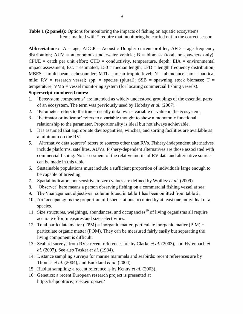
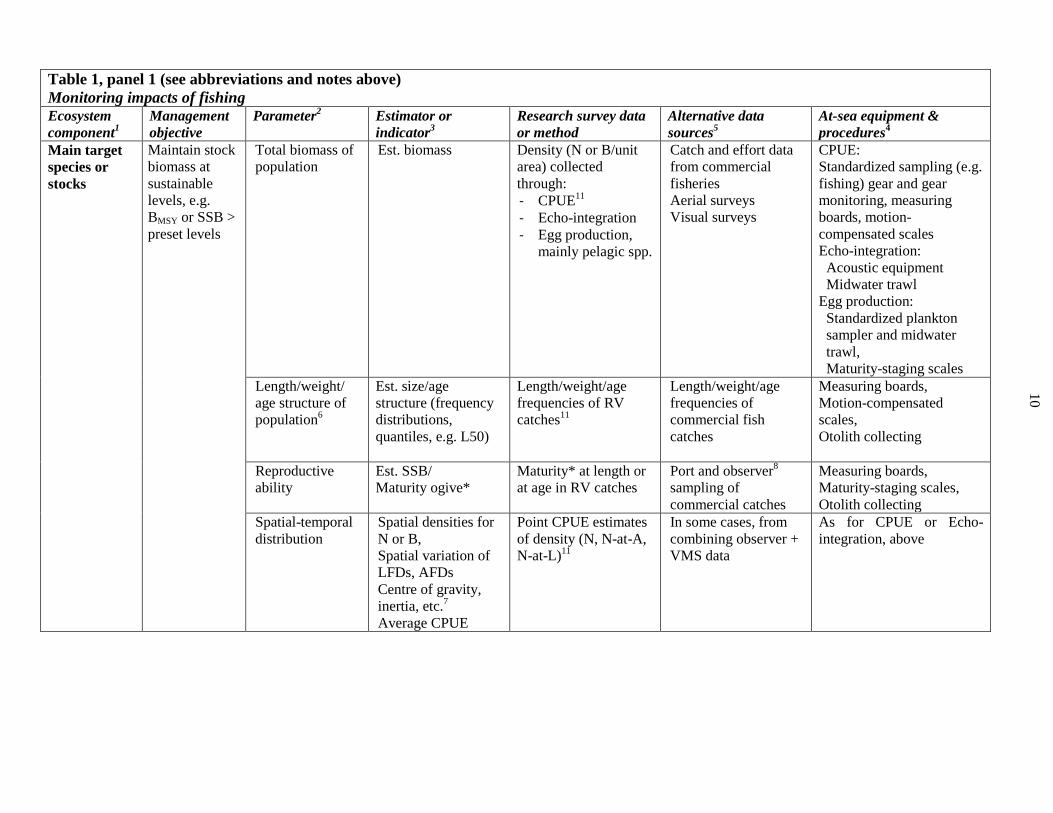
Table 1 (2 panels): Options for monitoring the impacts of fishing on aquatic ecosystems

Items marked with * require that monitoring be carried out in the correct season.

Abbreviations: A = age; ADCP = Acoustic Doppler current profiler; AFD = age frequency

distribution; AUV = autonomous underwater vehicle; B = biomass (total, or spawners only);

CPUE = catch per unit effort; CTD = conductivity, temperature, depth; EIA = environmental

impact assessment; Est. = estimated; L50 = median length; LFD = length frequency distribution;

MBES = multi-beam echosounder; MTL = mean trophic level; N = abundance; nm = nautical

mile; RV = research vessel; spp. = species (plural); SSB = spawning stock biomass; T =

temperature; VMS = vessel monitoring system (for locating commercial fishing vessels).

Superscript-numbered notes:

1. ‘Ecosystem components’ are intended as widely understood groupings of the essential parts

of an ecosystem. The term was previously used by Hobday et al. (2007).

2. ‘Parameter’ refers to the true – usually unknown – variable or value in the ecosystem.

3. ‘Estimator or indicator’ refers to a variable thought to show a monotonic functional

relationship to the parameter. Proportionality is ideal but not always achievable.

4. It is assumed that appropriate davits/gantries, winches, and sorting facilities are available as

a minimum on the RV.

5. ‘Alternative data sources’ refers to sources other than RVs. Fishery-independent alternatives

include platforms, satellites, AUVs. Fishery-dependent alternatives are those associated with

commercial fishing. No assessment of the relative merits of RV data and alternative sources

can be made in this table.

6. Sustainable populations must include a sufficient proportion of individuals large enough to

be capable of breeding.

7. Spatial indicators not sensitive to zero values are defined by Woillez et al. (2009).

8. ‘Observer’ here means a person observing fishing on a commercial fishing vessel at sea.

9. The ‘management objectives’ column found in table 1 has been omitted from table 2.

10. An ‘occupancy’ is the proportion of fished stations occupied by at least one individual of a

species.

11. Size structures, weighings, abundances, and occupancies10

of living organisms all require

accurate effort measures and size selectivities.

12. Total particulate matter (TPM) = inorganic matter, particulate inorganic matter (PIM) +

particulate organic matter (POM). They can be measured fairly easily but separating the

living component is difficult.

13. Seabird surveys from RVs: recent references are by Clarke et al. (2003), and Hyrenbach et

al. (2007). See also Tasker et al. (1984).

14. Distance sampling surveys for marine mammals and seabirds: recent references are by

Thomas et al. (2004), and Buckland et al. (2004).

15. Habitat sampling: a recent reference is by Kenny et al. (2003).

16. Genetics: a recent European research project is presented at

http://fishpoptrace.jrc.ec.europa.eu/

10

Table 1, panel 1 (see abbreviations and notes above)

Monitoring impacts of fishing

Ecosystem

component1

Management

objective

Parameter2

Estimator or

indicator3

Research survey data

or method

Alternative data

sources5

At-sea equipment &

procedures4

Main target

species or

stocks

Maintain stock

biomass at

sustainable

levels, e.g.

BMSY or SSB >

preset levels

Total biomass of

population

Est. biomass Density (N or B/unit

area) collected

through:

- CPUE11

- Echo-integration

- Egg production,

mainly pelagic spp.

Catch and effort data

from commercial

fisheries

Aerial surveys

Visual surveys

CPUE:

Standardized sampling (e.g.

fishing) gear and gear

monitoring, measuring

boards, motion-

compensated scales

Echo-integration:

Acoustic equipment

Midwater trawl

Egg production:

Standardized plankton

sampler and midwater

trawl,

Maturity-staging scales

Length/weight/

age structure of

population6

Est. size/age

structure (frequency

distributions,

quantiles, e.g. L50)

Length/weight/age

frequencies of RV

catches11

Length/weight/age

frequencies of

commercial fish

catches

Measuring boards,

Motion-compensated

scales,

Otolith collecting

Reproductive

ability

Est. SSB/

Maturity ogive*

Maturity* at length or

at age in RV catches

Port and observer8

sampling of

commercial catches

Measuring boards,

Maturity-staging scales,

Otolith collecting

Spatial-temporal

distribution

Spatial densities for

N or B,

Spatial variation of

LFDs, AFDs

Centre of gravity,

inertia, etc.7

Average CPUE

Point CPUE estimates

of density (N, N-at-A,

N-at-L)11

In some cases, from

combining observer +

VMS data

As for CPUE or Echo-

integration, above

11

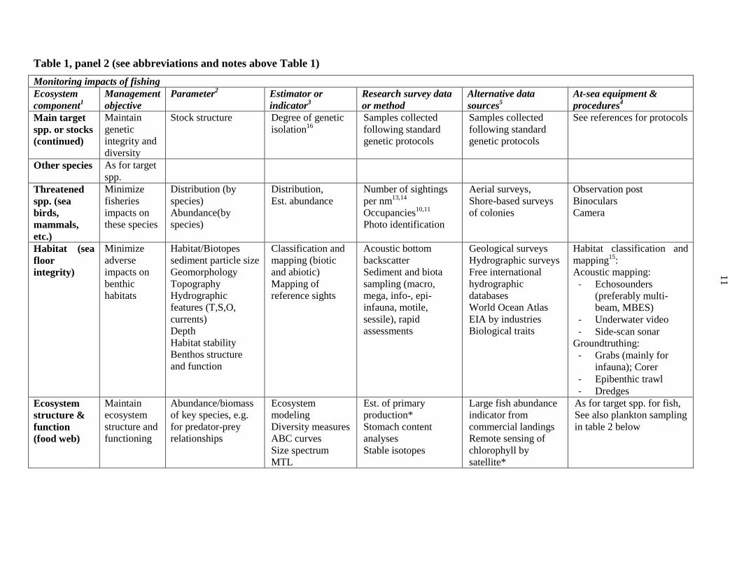
Table 1, panel 2 (see abbreviations and notes above Table 1)

Monitoring impacts of fishing

Ecosystem

component1

Management

objective

Parameter2

Estimator or

indicator3

Research survey data

or method

Alternative data

sources5

At-sea equipment &

procedures4

Main target

spp. or stocks

(continued)

Maintain

genetic

integrity and

diversity

Stock structure Degree of genetic

isolation16

Samples collected

following standard

genetic protocols

Samples collected

following standard

genetic protocols

See references for protocols

Other species As for target

spp.

Threatened

spp. (sea

birds,

mammals,

etc.)

Minimize

fisheries

impacts on

these species

Distribution (by

species)

Abundance(by

species)

Distribution,

Est. abundance

Number of sightings

per nm13,14

Occupancies10,11

Photo identification

Aerial surveys,

Shore-based surveys

of colonies

Observation post

Binoculars

Camera

Habitat (sea

floor

integrity)

Minimize

adverse

impacts on

benthic

habitats

Habitat/Biotopes

sediment particle size

Geomorphology

Topography

Hydrographic

features (T,S,O,

currents)

Depth

Habitat stability

Benthos structure

and function

Classification and

mapping (biotic

and abiotic)

Mapping of

reference sights

Acoustic bottom

backscatter

Sediment and biota

sampling (macro,

mega, info-, epi-

infauna, motile,

sessile), rapid

assessments

Geological surveys

Hydrographic surveys

Free international

hydrographic

databases

World Ocean Atlas

EIA by industries

Biological traits

Habitat classification and

mapping15

:

Acoustic mapping:

- Echosounders

(preferably multi-

beam, MBES)

- Underwater video

- Side-scan sonar

Groundtruthing:

- Grabs (mainly for

infauna); Corer

- Epibenthic trawl

- Dredges

Ecosystem

structure &

function

(food web)

Maintain

ecosystem

structure and

functioning

Abundance/biomass

of key species, e.g.

for predator-prey

relationships

Ecosystem

modeling

Diversity measures

ABC curves

Size spectrum

MTL

Est. of primary

production*

Stomach content

analyses

Stable isotopes

Large fish abundance

indicator from

commercial landings

Remote sensing of

chlorophyll by

satellite*

As for target spp. for fish,

See also plankton sampling

in table 2 below

12

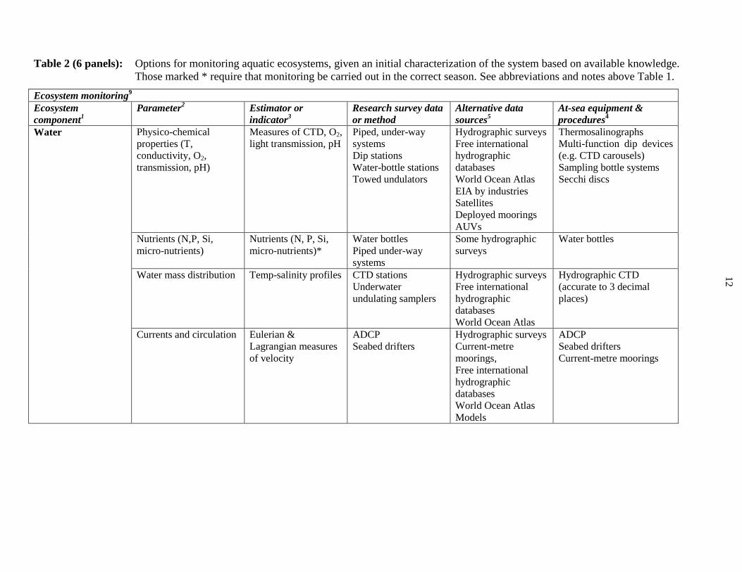
Table 2 (6 panels): Options for monitoring aquatic ecosystems, given an initial characterization of the system based on available knowledge.

Those marked * require that monitoring be carried out in the correct season. See abbreviations and notes above Table 1.

Ecosystem monitoring9

Ecosystem

component1

Parameter2

Estimator or

indicator3

Research survey data

or method

Alternative data

sources5

At-sea equipment &

procedures4

Water Physico-chemical

properties (T,

conductivity, O2,

transmission, pH)

Measures of CTD, O2,

light transmission, pH

Piped, under-way

systems

Dip stations

Water-bottle stations

Towed undulators

Hydrographic surveys

Free international

hydrographic

databases

World Ocean Atlas

EIA by industries

Satellites

Deployed moorings

AUVs

Thermosalinographs

Multi-function dip devices

(e.g. CTD carousels)

Sampling bottle systems

Secchi discs

Nutrients (N,P, Si,

micro-nutrients)

Nutrients (N, P, Si,

micro-nutrients)*

Water bottles

Piped under-way

systems

Some hydrographic

surveys

Water bottles

Water mass distribution

Temp-salinity profiles CTD stations

Underwater

undulating samplers

Hydrographic surveys

Free international

hydrographic

databases

World Ocean Atlas

Hydrographic CTD

(accurate to 3 decimal

places)

Currents and circulation Eulerian &

Lagrangian measures

of velocity

ADCP

Seabed drifters

Hydrographic surveys

Current-metre

moorings,

Free international

hydrographic

databases

World Ocean Atlas

Models

ADCP

Seabed drifters

Current-metre moorings

13

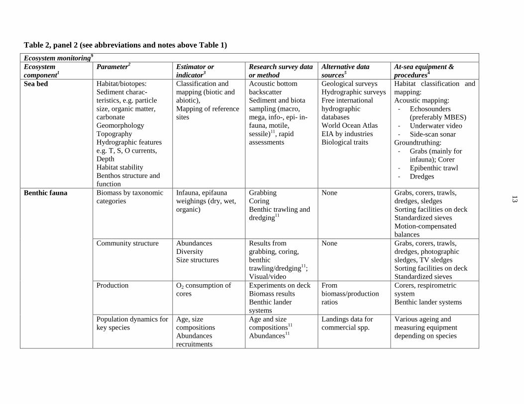
Table 2, panel 2 (see abbreviations and notes above Table 1)

Ecosystem monitoring9

Ecosystem

component1

Parameter2

Estimator or

indicator3

Research survey data

or method

Alternative data

sources5

At-sea equipment &

procedures4

Sea bed Habitat/biotopes:

Sediment charac-

teristics, e.g. particle

size, organic matter,

carbonate

Geomorphology

Topography

Hydrographic features

e.g. T, S, O currents,

Depth

Habitat stability

Benthos structure and

function

Classification and

mapping (biotic and

abiotic),

Mapping of reference

sites

Acoustic bottom

backscatter

Sediment and biota

sampling (macro,

mega, info-, epi- in-

fauna, motile,

sessile)11

, rapid

assessments

Geological surveys

Hydrographic surveys

Free international

hydrographic

databases

World Ocean Atlas

EIA by industries

Biological traits

Habitat classification and

mapping:

Acoustic mapping:

- Echosounders

(preferably MBES)

- Underwater video

- Side-scan sonar

Groundtruthing:

- Grabs (mainly for

infauna); Corer

- Epibenthic trawl

- Dredges

Benthic fauna Biomass by taxonomic

categories

Infauna, epifauna

weighings (dry, wet,

organic)

Grabbing

Coring

Benthic trawling and

dredging11

None Grabs, corers, trawls,

dredges, sledges

Sorting facilities on deck

Standardized sieves

Motion-compensated

balances

Community structure Abundances

Diversity

Size structures

Results from

grabbing, coring,

benthic

trawling/dredging11

;

Visual/video

None Grabs, corers, trawls,

dredges, photographic

sledges, TV sledges

Sorting facilities on deck

Standardized sieves

Production O2 consumption of

cores

Experiments on deck

Biomass results

Benthic lander

systems

From

biomass/production

ratios

Corers, respirometric

system

Benthic lander systems

Population dynamics for

key species

Age, size

compositions

Abundances

recruitments

Age and size

compositions11

Abundances11

Landings data for

commercial spp.

Various ageing and

measuring equipment

depending on species

14

Table 2, panel 3 (see abbreviations and notes above Table 1)

Ecosystem monitoring9

Ecosystem

component1

Parameter2

Estimator or indicator3

Research survey

data or method

Alternative data

sources5

At-sea equipment &

procedures4

Plankton Biomass of

phytoplankton

Phytoplankton

production

Species composition

Vertical and spatial

distribution

Biomass:

- Chlorophyll a /unit

volume

- Derived from

biomass & POC

Production:

- In situ or simulated

in situ incubations

Species composition:

- Microscopic

counts/unit vol.

- Spectral

composition/colour

Measures from

water bottles

Fluorescence

measures

In situ light levels

Remote sensing

satellites

Meteorological

information

Continuous

Plankton Recorder

(CPR)

Water bottles

Fluorescence metre

Incubation facilities

Microscopes

Optical plankton

counters

Towed optical systems

Analytical flow

cytometer (AFC)

Biomasses of

zooplankton

(categorized as micro,

meso, macro,

gelatinous)

Biomass:

- Wet & dry weights

by category/sizes

Production and

population dynamics for

key spp:

- Rate measures (e.g.

egg production,

moulting,

metabolism)

Species composition:

- Size spectrum

- Taxonomy

- Functional

groupings

Measures from

water bottles

Plankton nets

Optical systems

Acoustic systems

Stomach analyses of

zooplankton

grazers, e.g. small

pelagics

Coastal and moored

plankton stations

CPR

Water bottles

Plankton nets

Optical systems

Acoustic systems

Microscopes

Towed optical systems

Continuous under-way

fish egg sampler

15

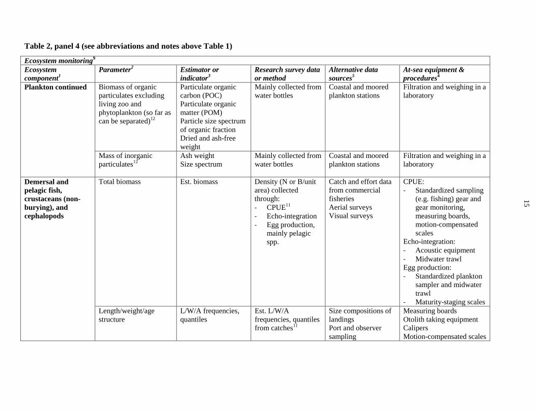
Table 2, panel 4 (see abbreviations and notes above Table 1)

Ecosystem monitoring9

Ecosystem

component1

Parameter2

Estimator or

indicator3

Research survey data

or method

Alternative data

sources5

At-sea equipment &

procedures4

Plankton continued Biomass of organic

particulates excluding

living zoo and

phytoplankton (so far as

can be separated)12

Particulate organic

carbon (POC)

Particulate organic

matter (POM)

Particle size spectrum

of organic fraction

Dried and ash-free

weight

Mainly collected from

water bottles

Coastal and moored

plankton stations

Filtration and weighing in a

laboratory

Mass of inorganic

particulates12

Ash weight

Size spectrum

Mainly collected from

water bottles

Coastal and moored

plankton stations

Filtration and weighing in a

laboratory

Demersal and

pelagic fish,

crustaceans (non-

burying), and

cephalopods

Total biomass Est. biomass Density (N or B/unit

area) collected

through:

- CPUE11

- Echo-integration

- Egg production,

mainly pelagic

spp.

Catch and effort data

from commercial

fisheries

Aerial surveys

Visual surveys

CPUE:

- Standardized sampling

(e.g. fishing) gear and

gear monitoring,

measuring boards,

motion-compensated

scales

Echo-integration:

- Acoustic equipment

- Midwater trawl

Egg production:

- Standardized plankton

sampler and midwater

trawl

- Maturity-staging scales

Length/weight/age

structure

L/W/A frequencies,

quantiles

Est. L/W/A

frequencies, quantiles

from catches11

Size compositions of

landings

Port and observer

sampling

Measuring boards

Otolith taking equipment

Calipers

Motion-compensated scales

16

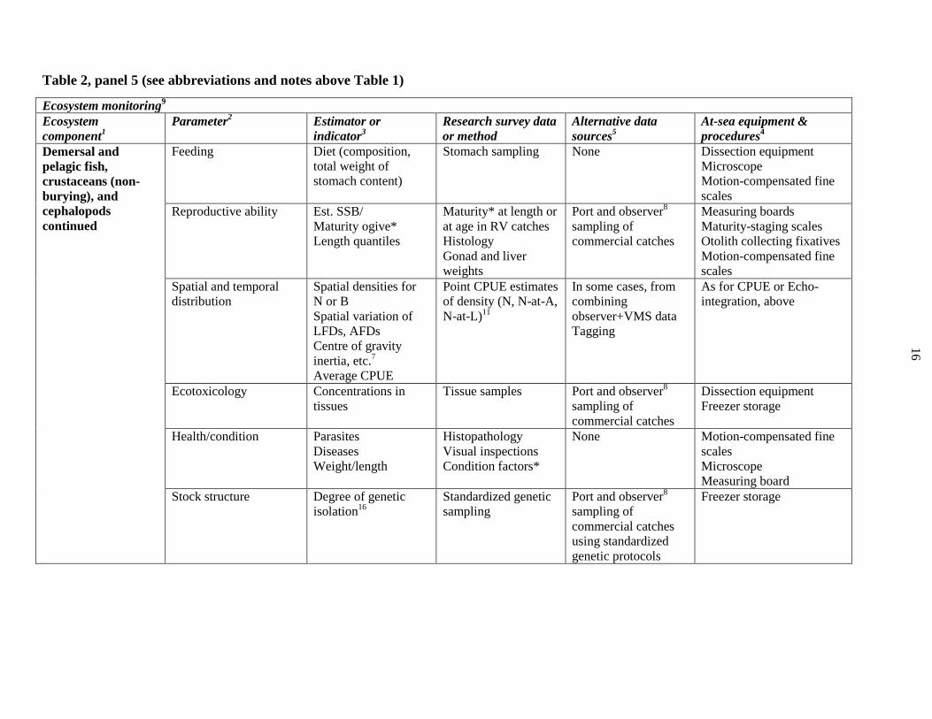
Table 2, panel 5 (see abbreviations and notes above Table 1)

Ecosystem monitoring9

Ecosystem

component1

Parameter2

Estimator or

indicator3

Research survey data

or method

Alternative data

sources5

At-sea equipment &

procedures4

Demersal and

pelagic fish,

crustaceans (non-

burying), and

cephalopods

continued

Feeding Diet (composition,

total weight of

stomach content)

Stomach sampling None Dissection equipment

Microscope

Motion-compensated fine

scales

Reproductive ability

Est. SSB/

Maturity ogive*

Length quantiles

Maturity* at length or

at age in RV catches

Histology

Gonad and liver

weights

Port and observer8

sampling of

commercial catches

Measuring boards

Maturity-staging scales

Otolith collecting fixatives

Motion-compensated fine

scales

Spatial and temporal

distribution

Spatial densities for

N or B

Spatial variation of

LFDs, AFDs

Centre of gravity

inertia, etc.7

Average CPUE

Point CPUE estimates

of density (N, N-at-A,

N-at-L)11

In some cases, from

combining

observer+VMS data

Tagging

As for CPUE or Echo-

integration, above

Ecotoxicology Concentrations in

tissues

Tissue samples

Port and observer8

sampling of

commercial catches

Dissection equipment

Freezer storage

Health/condition Parasites

Diseases

Weight/length

Histopathology

Visual inspections

Condition factors*

None Motion-compensated fine

scales

Microscope

Measuring board

Stock structure Degree of genetic

isolation16

Standardized genetic

sampling

Port and observer8

sampling of

commercial catches

using standardized

genetic protocols

Freezer storage

17

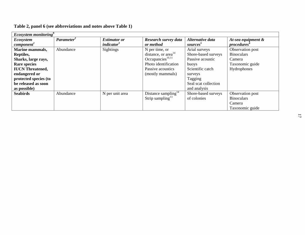
Table 2, panel 6 (see abbreviations and notes above Table 1)

Ecosystem monitoring9

Ecosystem

component1

Parameter2

Estimator or

indicator3

Research survey data

or method

Alternative data

sources5

At-sea equipment &

procedures4

Marine mammals,

Reptiles,

Sharks, large rays,

Rare species

IUCN Threatened,

endangered or

protected species (to

be released as soon

as possible)

Abundance Sightings N per time, or

distance, or area14

Occupancies10,11

Photo identification

Passive acoustics

(mostly mammals)

Arial surveys

Shore-based surveys

Passive acoustic

buoys

Scientific catch

surveys

Tagging

Seal scat collection

and analysis

Observation post

Binoculars

Camera

Taxonomic guide

Hydrophones

Seabirds Abundance N per unit area Distance sampling14

Strip sampling13

Shore-based surveys

of colonies

Observation post

Binoculars

Camera

Taxonomic guide

18

REFERENCES

Buckland, S.T., Andersen, D.R., Burnham, K.P., Laake, J.L., Borchers, D.L. & Thomas, L. 2004. Advanced distance sampling. Oxford University Press, Oxford, UK. 430 pp.

Clarke, E.D., Spear, L.B., McCracken, M.L., Marques, F.F.C., Borchers, D.L., Buckland,

S.T. & Ainley, D.G. 2003. Validating the use of generalized additive models and at-sea

surveys to estimate size and temporal trends of seabird populations. Journal of Applied

Ecology 40, pp. 278–292.

Cotter, J. & Lart, W. 2011. A guide for ecological risk assessment of the effects of commercial

fishing (ERAEF). Sea Fish Industry Authority, Grimsby, UK, 78pp.

http://sin.seafish.org/portal/site/sin/

Hobday, A. J., Smith, A. Webb, H., Daley, R., Wayte, S., Bulman, C., Dowdney, J., Williams,

A., Sporcic, M., Dambacher, J., Fuller M. & Walker, T. 2007. Ecological Risk

Assessment for the Effects of Fishing: Methodology. Report R04/1072 for the Australian

Fisheries Management Authority, Canberra. No. Report R04/1072, 174 pp.

www.afma.gov.au

Hyrenbach, K.D., Henry, M.F., Morgan, K.H., Welch, D.W. & Sydeman, W.J. 2007.

Optimizing the width of strip transects for seabird surveys from vessels of opportunity.

Marine Ornithology 35, 29–38.

Kenny, A.J., Cato, I., Desprez, M., Fader, G., Schüttenhelm, R.T.E. & Side, J. 2003. An

overview of seabed-mapping technologies in the context of marine habitat classification.

ICES Journal of Marine Science 60, 411–418.

Tasker, M.L., Hope Jones, P., Dixon, T. & Blake, B.F. 1984. Counting Seabirds at Sea from

Ships: A Review of methods employed and a suggestion for a standardized approach.

American Ornithologists Union (Auk), Vol. 101 Issue 3, pp. 567–577

Thomas, L., Burnham, K.P. & Buckland, S.T. 2004. Temporal inferences from distance

sampling surveys. In: Advanced distance sampling. (Eds. Buckland, S.T., Andersen, D.R.,

Burnham, K.P., Laake, J.L., Borchers, D.L. & Thomas, L). Oxford University Press, UK.

pp. 71–107.

Woillez, M., Rivoirard, J. & Petigas, P. 2009. Notes on survey-based spatial indicators for

monitoring fish populations. Aquatic Living Resources 22, 155–164.

19

Appendix I: List of Participants

John COTTER

Director

FishWorld Science Ltd

57 The Avenue

Lowestoft NR33 7LH

UNITED KINGDOM

Tel.: +44 (0)1502 564 541

E-mail: john.cotter@phonecoop.coop

www.fishworldscience.com

Abdelmalek FARAJ

Chef du Département des Ressources

Halieutiques

Institut National de Recherche Halieutique

(INRH)

2, rue de Tiznit

Casablanca

20000 MOROCCO

Tel.: +212 522 22 02 49

E-mail: faraj@inrh.org.ma

Paulus KAINGE

National Marine Information and Research

Centre

Ministry of Fisheries and Marine Resources

Strand Street, PO Box 912

Swakopmund

NAMIBIA

Tel.: +264 64 4101000

E-mail: pkainge@mfmr.gov.na

Andrew KENNY

Centre for Environment, Fisheries &

Aquaculture Science (CEFAS)

Pakefield Road

Lowestoft

Suffolk NR33 0HT

UNITED KINGDOM

Tel.: +44 (0)1502 562244

E-mail: Andrew.kenny@cefas.co.uk

Kathrine MICHALSEN

Institute of Marine Research (IMR)

P.O. Box 1870 Nordnes

5817 Bergen

NORWAY

Tel.: +47 55 23 85 00

E-mail: kathrine.michalsen@imr.no

www.imr.no

Christian MÖLLMANN

Institute for Hydrobiology and Fisheries

Science

University of Hamburg

Grosse Elbstrasse 133

D-22767 Hamburg

GERMANY

Tel.: +49 40 42838 6621

E-mail: christian.moellmann@uni-hamburg.de

Ana RAMOS

Instituto Español de Oceanografía (IEO)

Cabo Estai, Canido

36200, Vigo (Pontevedra)

SPAIN

Tel: +34 986 492111

Email: ana.ramos@vi.ieo.es

www.ieo.es

David REID

International Council for the Exploration of

the Sea (ICES)

Marine Institute

Rinville, Oranmore

Co Galway

IRELAND

Tel.: +353 91 387431

E-mail: david.reid@marine.ie

20

Claude ROY

Directeur

Laboratoire de Physique des Océans (LPO)

Centre Ifremer de Brest

B.P. 70, 29280 Plouzané

FRANCE

Tel.: +33 2 98 22 4500/4276

Cell.: +33 6 60 83 6337

E-mail: claude.roy@ird.fr

www.ifremer.fr/lpo

Somboon SIRIRAKSOPHON

Policy and Program Coordinator

Southeast Asian Fisheries Development

Center (SEAFDEC)

Department of Fisheries

Ladyao, Chatuchak

Bangkok 10900, THAILAND

Tel.: +66 2940 6332/6326 Ext. 111

Cell.: +66 8 9477 9968

E-mail: somboon@seafdec.org/

ssiriraksophon63@gmail.com

Hein Rune SKJOLDAL

Institute of Marine Research (IMR)

P.O. Box 1870 Nordnes

5817 Bergen

NORWAY

Tel.: +47 55 23 85 00

E-mail: hein.rune.skjoldal@imr.no

www.imr.no

Tore STROMME

Research Coordinator, EAF-Nansen Project

Institute of Marine Research (IMR)

P.O. Box 1870 Nordnes

5817 Bergen, Norway

Tel.: +39 06 5705 4735

E-mail: tore.stromme@fao.org

FAO

Gabriella BIANCHI

Service Coordinator

Marine and Inland Fisheries Service (FIRF)

Fisheries and Aquaculture Department

Via delle Terme di Caracalla

00153 Rome, Italy

Tel.: +39 06 5705 3094

E-mail: gabriella.bianchi@fao.org

Kevern COCHRANE

Director

Fisheries and Aquaculture Resources Use

and Conservation Division (FIR)

Via delle Terme di Caracalla

00153 Rome, Italy

Tel.: +39 06 5705 6109

E-mail: kevern.cochrane@fao.org

Kwame KORANTENG

EAF Coordinator

Fisheries and Aquaculture Department

Via delle Terme di Caracalla

00153 Rome, Italy

Tel.: +39 06 5705 6007

E-mail: kwame.koranteng@fao.org

Merete TANDSTAD

Fishery Resources Officer

Marine and Inland Fisheries Service (FIRF)

Fisheries and Aquaculture Department

Via delle Terme di Caracalla

00153 Rome, Italy

Tel.: +39 06 5705 2019

E-mail: merete.tandstad@fao.org

21

Appendix II: Provisional Agenda

DAY 1 (Monday, 29 August 2011):

09.00 Opening

o Opening remarks by Dr Kevern Cochrane, Director FIRX

o Introduction

o Election of Chairs/Moderators and Rapporteurs

o Adoption of the Agenda

o Objectives of the expert workshop (Gabriella Bianchi)

o Brief introductory remarks by experts

10.30 Morning Tea / Coffee

10.50 Presentation of the background review paper

o Discussions

12.30 Lunch

13.30 o Discussions

15.00 Afternoon Tea / Coffee

15.20 o General discussions and additional information by participants on their

experiences in developing and using ecosystem indicators, especially in fisheries

science and management

17.00 Close of Day 1 sessions

DAY 2 (Tuesday, 30 August 2011)

09.00 o Defining ecosystem survey objectives

10.30 Morning Tea / Coffee

10.50 o Examination of list of issues and indicators

13.00 Lunch

14.00 o Determining the indicators and defining reference points vis-à-vis the

objectives

15.30 Afternoon Tea / Coffee

15.50 o Identifying what issues might arise in the use and presentation of these

indicators for management

17.00 Close of Day 2

22

DAY 3 (Wednesday 31 August 2011)

09.00 o Vessel and human capability required to undertake ecosystem surveys

10.30 Morning Tea / Coffee

11.00 o Discussions

12.30 Lunch

13.30

o Providing advice

a framework for research priorities that can be addressed by ecosystem

surveys

Revision of the background paper and the best format in which to publish it

What types of outputs are needed for whom and what form and structure

should they take?

15.30 Afternoon Tea / Coffee

16.00 o Outstanding issues

16.30 Closing of workshop

DRAFT 28 OCT 2011

1

USING RESEARCH VESSELS FOR AN ECOSYSTEM APPROACH TO FISHERIES

Draft paper produced following an expert workshop, 29-31 August 2011

Food and Agriculture Organization of the United Nations,

Rome, Italy

Prepared 28 October 2011 by

JOHN COTTER

c/o FishWorld Science Ltd

57 The Avenue

Lowestoft

United Kingdom NR33 7LH

Tel. +44 (0) 1502 564 541

john.cotter@phonecoop.coop

www.fishworldscience.com

CONTENTS

2

CONTENTS

Acknowledgements................................................................................................................................. 5

Table of figures.........................................................................................................................................6

Table of tables...........................................................................................................................................6

Glossary.....................................................................................................................................................7

SUMMARY............................................................................................................................................11

1 INTRODUCTION .......................................................................................................................... 14

2 PLANNING AN RV ECOSYSTEM MONITORING SURVEY (EMS) ............................. 19

2.1 Defining the ecosystem to be monitored .................................................................................... 21

2.2 Developing a knowledge base ..................................................................................................... 22

2.3 Which ecosystem components?................................................................................................... 23

2.3.1 Seawater .................................................................................................................................... 28

2.3.2 Zooplankton and phytoplankton ............................................................................................. 28

2.3.3 Jellyplankton ............................................................................................................................. 29

2.3.4 Cephalopods ............................................................................................................................. 30

2.3.5 Pelagic fish................................................................................................................................ 30

2.3.6 Demersal fish ............................................................................................................................ 31

2.3.7 Sharks, skates and rays ............................................................................................................ 32

2.3.8 Epibenthos ................................................................................................................................ 32

2.3.9 Infauna ...................................................................................................................................... 33

2.3.10 Seafloor habitats ................................................................................................................... 33

2.3.11 Communities ........................................................................................................................ 38

2.3.12 Seabirds ................................................................................................................................ 38

2.3.13 Mammals .............................................................................................................................. 38

2.3.14 Reptiles ................................................................................................................................. 39

2.3.15 Conclusions .......................................................................................................................... 39

2.4 What sort of research vessel (RV)? ............................................................................................. 40

2.4.1 An RV shared with a groundfish survey (GFS) ..................................................................... 43

CONTENTS

3

2.4.2 An RV shared with an acoustic survey ................................................................................... 44

2.4.3 A purpose-built RV .................................................................................................................. 44

2.4.4 Chartered fishing vessels as RVs ............................................................................................ 45

2.4.5 Multiple RVs ............................................................................................................................ 47

2.4.6 Conclusions .............................................................................................................................. 48

2.5 What sort of ecosystem sampling devices? ................................................................................ 49

2.5.1 Water sampling ........................................................................................................................ 53

2.5.2 Plankton sampling .................................................................................................................... 53

2.5.3 Trawling for fish ....................................................................................................................... 54

2.5.4 Epibenthic trawling and dredging ........................................................................................... 55

2.5.5 Benthic grabbing and coring ................................................................................................... 56

2.5.6 Active acoustic techniques ...................................................................................................... 56

2.5.7 Passive acoustic techniques ..................................................................................................... 56

2.5.8 Sight surveys ............................................................................................................................ 57

2.5.9 Conclusions .............................................................................................................................. 57

3 ECOSYSTEM SURVEY DESIGN ............................................................................................. 59

3.1 Choosing the survey domain ....................................................................................................... 60

3.2 Statistical terms and inference ..................................................................................................... 64

3.3 Station-based sampling ................................................................................................................ 64

3.4 Design-based regional estimation ............................................................................................... 65

3.5 Model-based estimation with a grid of stations .......................................................................... 70

3.6 A compromise design: a lattice of strata ..................................................................................... 71

3.7 Conclusions ................................................................................................................................... 72

4 PROCESSING CATCHES AT SEA .......................................................................................... 74

4.1 Cleaning the catch ........................................................................................................................ 76

4.2 Separating species ........................................................................................................................ 76

4.3 Sampling species‟ catches for length-frequencies (LFDs) ....................................................... 79

CONTENTS

4

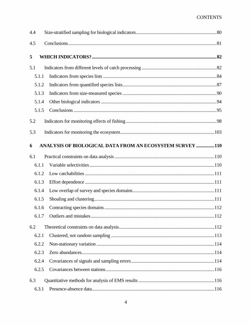
4.4 Size-stratified sampling for biological indicators ....................................................................... 80

4.5 Conclusions ................................................................................................................................... 81

5 WHICH INDICATORS? .............................................................................................................. 82

5.1 Indicators from different levels of catch processing .................................................................. 82

5.1.1 Indicators from species lists .................................................................................................... 84

5.1.2 Indicators from quantified species lists ................................................................................... 87

5.1.3 Indicators from size-measured species ................................................................................... 90

5.1.4 Other biological indicators ...................................................................................................... 94

5.1.5 Conclusions .............................................................................................................................. 95

5.2 Indicators for monitoring effects of fishing ................................................................................ 98

5.3 Indicators for monitoring the ecosystem ................................................................................... 103

6 ANALYSIS OF BIOLOGICAL DATA FROM AN ECOSYSTEM SURVEY ................ 110

6.1 Practical constraints on data analysis ........................................................................................ 110

6.1.1 Variable selectivities .............................................................................................................. 110

6.1.2 Low catchabilities .................................................................................................................. 111

6.1.3 Effort dependence .................................................................................................................. 111

6.1.4 Low overlap of survey and species domains ........................................................................ 111

6.1.5 Shoaling and clustering .......................................................................................................... 111

6.1.6 Contracting species domains ................................................................................................. 112

6.1.7 Outliers and mistakes ............................................................................................................. 112

6.2 Theoretical constraints on data analysis .................................................................................... 112

6.2.1 Clustered, not random sampling ........................................................................................... 113

6.2.2 Non-stationary variation ........................................................................................................ 114

6.2.3 Zero abundances ..................................................................................................................... 114

6.2.4 Covariances of signals and sampling errors ......................................................................... 114

6.2.5 Covariances between stations ................................................................................................ 116

6.3 Quantitative methods for analysis of EMS results ................................................................... 116

6.3.1 Presence-absence data ............................................................................................................ 116

CONTENTS

5

6.3.2 Ordered categorical data ........................................................................................................ 117

6.3.3 Ranked data ............................................................................................................................ 117

6.3.4 Real-valued measures ............................................................................................................ 118

6.3.5 Analysis of habitat indicators ................................................................................................ 119

6.3.6 Community indicators ........................................................................................................... 120

6.4 Conclusions ................................................................................................................................. 120

7 APPLYING EMS RESULTS FOR AN EAF MANAGEMENT ......................................... 122

8 CHECKLIST FOR AN RV ECOSYSTEM SURVEY .......................................................... 125

9 REFERENCES ............................................................................................................................. 127

Acknowledgements

This report, funded by FAO FIRF, was developed from a background paper prepared for an FAO

expert workshop, held in Rome from 29 to 31 August 2011, on use of RVs to build a knowledge base

for EAF. It benefits considerably from discussions at that workshop. Other participants were

Merete Tandstad, Claude Roy, Abdelmalek Faraj, Ana Ramos, Paulus Kainge, Torre Stromme,

Andrew Kenny, Christian Moellman, Dave Reid, Kathrine Michalsen, Hein Rune Skjoldal,

Somboon Siriraksophon, Gabriella Bianchi, and Kwame Koranteng. Other acknowledgements are

for experience gained in ecosystem sampling on GFSs around UK with Simon Jennings, Ruth

Zuhlke=Callaway, and Jim Ellis of Cefas; for patient coaching in catch-sampling by several Cefas

RV scientists, on the EC funded FISBOAT project concerning RV surveys; and on ecological risk

assessment for effects of fishing with Bill Lart of Seafish Industry Authority, Grimsby. This report is

the responsibility of the author only and does not contain any official views.

CONTENTS

6

TABLE OF FIGURES

Figure 1.1 How an EMS might fit into an EAF management. .............................................................. 17

Figure 2.1 Schematic diagram depicting initial planning of an EMS. ................................................... 20

Figure 3.1. Effects of migrations on relationship of a survey domain to a species domain ............... 62

Figure 3.2. Aliasing of a systematic, one dimensional sampling grid .................................................. 71

Figure 4.1 Scheme for initial cleaning and sorting of an RV trawl catch. ............................................ 75

Figure 4.2. Scheme for separating a mix of two imaginary, look-alike species ................................... 78

Figure 4.3. Estimating a length frequency distribution by length-stratified random sampling ........... 80

Figure 5.1 A suggested catch processing scheme. ................................................................................. 83

Figure 5.2. Occupancies for selected, contrasting species, EGFS of the North Sea.. ........................... 86

Figure 5.3. Two length-based community indicators, EGFS of the North Sea .................................... 93

Figure 6.1. To illustrate a cluster sample .............................................................................................. 113

TABLE OF TABLES

Table 1.1. Differences between GFSs and EMS, both using RVs.. ...................................................... 18

Table 2.1 Selected components of marine ecosystems, reasons for monitoring in EAF. ................... 24

Table 2.2. Keywords for classifying substrate types of seafloor habitats. .................................... 35

Table 2.3. Keywords for classifying geomorphic forms of seafloor habitats.................................. 36

Table 2.4. Keywords for classifying non-mobile benthic life on the seafloor. ................................. 37

Table 2.5. Types of RV suitable for an EMS. ......................................................................................... 41

Table 2.6 Ecosystem sampling techniques deployable from an RV. .................................................... 50

Table 3.1 List of fields for a Species database to support an EMS. ...................................................... 63

Table 5.1. Various spatial indicators. ....................................................................................................... 90

Table 5.2. Hierarchy of sampling a demersal fishing trawl on an EMS. ............................................... 97

Table 5.3. Hierarchy of sampling an epibenthic trawl on an EMS ........................................................ 97

Table 5.4 Options for monitoring the impacts of fishing on aquatic ecosystems. ............................... 99

Table 5.5 Options for monitoring aquatic ecosystems .......................................................................... 104

GLOSSARY

7

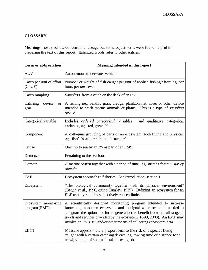
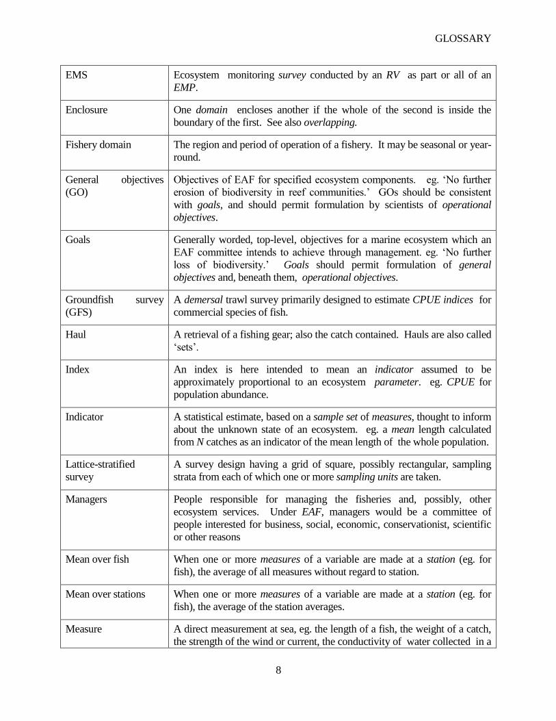
GLOSSARY

Meanings mostly follow conventional useage but some adjustments were found helpful in

preparing the text of this report. Italicized words refer to other entries.

Term or abbreviation Meaning intended in this report

AUV Autonomous underwater vehicle

Catch per unit of effort

(CPUE)

Number or weight of fish caught per unit of applied fishing effort, eg. per

hour, per nm towed.

Catch sampling Sampling from a catch on the deck of an RV

Catching device or

gear

A fishing net, benthic grab, dredge, plankton net, corer or other device

intended to catch marine animals or plants. This is a type of sampling

device.

Categorical variable Includes ordered categorical variables and qualitative categorical

variables, eg. „red, green, blue‟.

Component A colloquial grouping of parts of an ecosystem, both living and physical.

eg. „fish‟, „seafloor habitat‟, „seawater‟.

Cruise One trip to sea by an RV as part of an EMS.

Demersal Pertaining to the seafloor.

Domain A marine region together with a period of time. eg. species domain, survey

domain

EAF Ecosystem approach to fisheries. See Introduction, section 1

Ecosystem “The biological community together with its physical environment”

(Begon et al., 1996, citing Tansley, 1935). Defining an ecosystem for an

EAF usually requires subjectively chosen limits.

Ecosystem monitoring

program (EMP)

A scientifically designed monitoring program intended to increase

knowledge about an ecosystem and to signal when action is needed to

safeguard the options for future generations to benefit from the full range of

goods and services provided by the ecosystem (FAO, 2003). An EMP may

involve an RV EMS and/or other means of collecting ecosystem data.

Effort Measure approximately proportional to the risk of a species being

caught with a certain catching device. eg. towing time or distance for a

trawl, volume of sediment taken by a grab.

GLOSSARY

8

EMS Ecosystem monitoring survey conducted by an RV as part or all of an

EMP.

Enclosure One domain encloses another if the whole of the second is inside the

boundary of the first. See also overlapping.

Fishery domain The region and period of operation of a fishery. It may be seasonal or year-

round.

General objectives

(GO)

Objectives of EAF for specified ecosystem components. eg. „No further

erosion of biodiversity in reef communities.‟ GOs should be consistent

with goals, and should permit formulation by scientists of operational

objectives.

Goals Generally worded, top-level, objectives for a marine ecosystem which an

EAF committee intends to achieve through management. eg. „No further

loss of biodiversity.‟ Goals should permit formulation of general

objectives and, beneath them, operational objectives.

Groundfish survey

(GFS)

A demersal trawl survey primarily designed to estimate CPUE indices for

commercial species of fish.

Haul A retrieval of a fishing gear; also the catch contained. Hauls are also called

„sets‟.

Index An index is here intended to mean an indicator assumed to be

approximately proportional to an ecosystem parameter. eg. CPUE for

population abundance.

Indicator A statistical estimate, based on a sample set of measures, thought to inform

about the unknown state of an ecosystem. eg. a mean length calculated

from N catches as an indicator of the mean length of the whole population.

Lattice-stratified

survey

A survey design having a grid of square, possibly rectangular, sampling

strata from each of which one or more sampling units are taken.

Managers People responsible for managing the fisheries and, possibly, other

ecosystem services. Under EAF, managers would be a committee of

people interested for business, social, economic, conservationist, scientific

or other reasons

Mean over fish When one or more measures of a variable are made at a station (eg. for

fish), the average of all measures without regard to station.

Mean over stations When one or more measures of a variable are made at a station (eg. for

fish), the average of the station averages.

Measure A direct measurement at sea, eg. the length of a fish, the weight of a catch,

the strength of the wind or current, the conductivity of water collected in a

GLOSSARY

9

bottle.

nm Nautical mile

Occupancy The proportion of stations fished at which at least one individual of a

species is present.

Operational objective

(OO)

Detailed objectives of EAF for individual units of specified ecosystem

components. eg. „CPUE of mature individuals of Species X to be > Y

kg.hr-1

.‟ OOs should be consistent with general objectives and, above

them, goals.

Ordered categorical

variable

A set of intervals that can be ordered by magnitude, eg. „Lo, Med, Hi‟, „0 –

5, 6 -10, 11 – 20‟

Overlapping One domain is said to overlap another if they share some time and space

but neither totally encloses the other. [Elsewhere, overlap includes

enclosure, but not in this report.]

Pelagic Pertaining to mid and surface waters

Percentile A quantile written in percentage terms, with 0 100p

Presence-absence

variable

Binary number: 0 = absent, 1 = present, ie. one or more.

Quantile The value, py , of a variable, y, is said to be the p‟th quantile of a

population when a proportion, p, exhibits values of y less than or equal to

py ; eg. the median, 0.5y . Quantiles estimated from samples must allow

for n odd or even. See also percentile.

Randomly located

station

One whose longitude and latitude co-ordinates are each drawn from a

uniform statistical density function enclosing the stratum or survey domain.

Co-ordinates falling outside the domain are not used.

Region A bounded area of sea

Research vessel (RV) A vessel allocated for taking samples and making measurements at sea

independently of any fishery or of other commercial pressures so that all

work can be conducted to objective, scientific standards. At least one of

the crew should be scientifically trained.

Sample A sample set or a sampling unit. The term has been avoided when there

can be ambiguity.

Sample set A set of N sampling units.

Sampling Process of removing sampling units from a population or substance for

scientific purposes. The „population‟ might be in the sea, or a catch on

GLOSSARY

10

deck.

Sampling device A device designed to collect or observe any part of an ecosystem. Includes

a catching device.

Sampling domain That part of the survey domain that is accessible to a specified sampling

device.

Sampling unit The smallest unit of a sampling task, eg. one haul of a net, one retrieval of a

grab, one value read from a dipped electrode, one bottle of seawater, one

basket of fish from a catch.

Selectivity Size selectivity: mathematical function of size (usually length) for a

specified species that measures the proportion of individuals that are

exposed to a catching device and caught. Species selectivity: How many

species are caught by a catching device.

Set See haul

Species domain The region occupied by a species and the period when it is present. It may

vary seasonally because of migrations or life history.

Station Any marine sampling location, defined by longitude, latitude, time and

depth marking the start and end, or just the mid-point, of the tow or dip.

Stratum (plural=strata) A defined part of a survey domain.

Survey One repetition of all monitoring tasks at all stations for an EMS. Often a

survey is completed with one cruise by one RV.

Survey domain The region surveyed by an RV together with the seasonal period of each

survey .

TEP species Threatened, endangered or protected species. Also known as „PETs‟.

Unit The smallest relevant part of an ecosystem component. See Introduction,

section 1.

SUMMARY

11

SUMMARY

An ecosystem monitoring survey (EMS) conducted by a research vessel (RV) for the purpose

of an ecosystem approach to fisheries management is more complicated than a groundfish survey

(GFS) focused primarily on commercial fish species. An EMS survey must deal with many more

species, perhaps hundreds, most of which are not demersal fish. More than one type of gear with

different catching powers is likely to be fished and many species will not be caught well by any of

them. Some species will be enclosed by the survey, others only partially. Supplementary sampling

techniques may include seabird sight surveys and acoustic monitoring of habitat structure.

Conducting all of these activities on a single RV makes special demands for deckspace, laboratory

cabins, scheduling, cruise planning and so on. An EMS can feasibly monitor many ecosystem

components including: water, plankton, jellyplankton, pelagic fish, demersal fish and skates and rays

depending on the type of trawl used, attached and mobile epibenthos, infauna, seafloor habitats, and

seabirds. Components less suited for RV monitoring are ctenophores, cephalopods, pelagic sharks,

marine mammals, sea turtles, and sea snakes.

Several types of vessel can be used for ecosystem work. A low-cost, somewhat constrained

option is to combine the EMS with a GFS already undertaken for assessing commercial stocks. A

purpose-built RVs is expensive and offers the most on-board facilities for an EMS but it may not, in

fact, be needed for all EMS work, or it may be too big to visit shallow waters. Chartered fishing

vessels are cheaper RVs but suffer from limited deck space, lively sea motion, lack of height for sight

surveys, and uncontrolled modifications by the owner that can create intercalibration problems from

year to year. Random selection of vessels from a fishing fleet is suggested to get around

intercalibration problems. Multiple RVs can be co-ordinated for an ecosystem survey allowing

sampling over wider areas and at different places.

Sampling techniques for an EMS may include demersal trawling, oceanographic and plankton

sampling, acoustic techniques such as echosounders and sidescan sonar for monitoring benthic

habitats, grabbing, beam trawling, dredging, sight surveys for seabirds, mammals and, possibly,

jellyplankton. Passive acoustic listening to vocal marine animals awaits development of routine

techniques. All sampling methods required detailed protocols so that different scientific crews can

standardize their work on every RV monitoring cruise. Taxonomic skills and thorough training in all

sampling techniques are critical for EMSs. The occurrence of confusable species should be expected

and dealt with by naming them in standard ways.

SUMMARY

12

Bounding the survey domain before designing the survey should take into account the

distributions of priority species and could be assisted by a „Species database‟ holding distributions,

migrations, and habitat preferences for each species. Boundaries should also take into account

feasibility of sampling on different types of seafloor by different gears. The season of an EMS must

be carefully chosen because many indicators are sensitive to seasonal growth, temperature,

migrations, and reproductive cycles. Different catching devices are unlikely to be intercalibrated for

different catchabilities for each species, implying that caution is needed when interpreting

multispecies data from an EMS.

Replicate sampling at individual stations is not recommended because of the environmental

heterogeneity and the need to spread stations widely. Instead, regional estimation with design-based,

randomized sampling schemes is proposed. Sampling may be stratified so that evenness of coverage

is better than for simple random sampling, or so that major features of the ecosystem, eg. different

habitats, are focussed on if this is thought to be more informative for EAF. The number of strata

should be low with many stations in each for maximum precision and dependability of EMS results.

Model-based estimation is proposed when EMS results will be analysed by fitting a model, eg.

contours. A regular grid of stations then provides equal densities of information for fitting the model.

Grids may estimate summarizing statistics, eg. the mean, with bias. Another design, lattice-stratified

with one station per square stratum is put forward as a compromise reasonably good for both regional

estimation and modelling.

The processing of catches, whether from the main trawl or some other catching device must

be planned to suit the space, time, and scientific crew available. Protocols are essential for every

gear. Depending on facilities on board, catch processing generally involves firstly, species

identification, then quantification, then length measurements and, finally, additional sampling for

biological measures. Catch-based indicators can be graded to correspond to these different levels of

processing.

Indicators for species lists include occupancies, spatial positive area, and the Bayesian

occupancy index (BOI). They appear to be particularly suitable for rare and poorly catchable

species. CPUE-based indicators for many non-commercial species are likely to be poorly measured

because of poor catchabilities and other reasons. A priori groupings of species by expected

sensitivities to fishing or other factors is important for reducing the number of potentially confusing

trends when examining CPUE time series. Intrinsic population growth rate, spatial indicators, and

SUMMARY

13

multivariate techniques can smooth them and reduce their dimensionality. The threat index assesses

extinction risk from survey CPUEs. The L25, L50, and L75 (or other) length quantiles reduce the

multi-dimensionality of length-frequency distributions while still distinguishing recruiting classes

from newly mature animals and older broodstock. Sizes can be used to create composite community

indicators that have been shown to vary over time, probably as a result of fishing. Weight-at-length

or bodily condition can indicate growing conditions and perhaps density-dependent effects of strong

year classes. Reproductive indicators should only be assessed by RV surveys occurring in the

months just before spawning. Length- or age-at-maturity is useful for estimating breeding

proportions in a population. A large table lists indicators alongside the several groupings of

ecosystem components for monitoring and managing the effects of commercial fisheries. Another

lists indicators and components for monitoring the ecosystem. The tables put forward options;

monitoring of all of them would require considerable RV resources. drawn up by the FAO expert

committee on using RVs for EAF

Several theoretical and practical constraints should be considered when analysing EMS data.

Many statistical and modelling methods are available for ecosystem measures. They differ in the

assumptions needed. Changes in habitat quality may be related to changes of fishing effort by

quadrat using a nonparametric correlation method. Community indicators can mostly be calculated

from abundance, size, and weight data collected by an ecosystem survey.

The report is finished with notes on applying EMS results for an EAF management. The

reference point, and ecological risk assessment methods are briefly described. A short check-list of

items to consider when planning an ecosystem survey is also given.

1. INTRODUCTION

14

1 INTRODUCTION

An „Ecosystem Approach to Fisheries‟ (EAF) according to the Food and Agriculture

Organization of the United Nations (FAO, 2003):

‘strives to balance diverse societal objectives, by taking account of the knowledge and

uncertainties of biotic, abiotic and human components of ecosystems and their interactions and

applying an integrated approach to fisheries within ecologically meaningful boundaries.’

Its purpose

‘is to plan, develop and manage fisheries in a manner that addresses the multiple needs and

desires of societies, without jeopardizing the options for future generations to benefit from the full

range of goods and services provided by marine ecosystems.’

FAO has also advised on responsible fishing (FAO, 1995), further on the EAF itself (FAO,

2005), on indicators for sustainable development of marine fisheries (FAO, 1999), and on ecosystem

modelling (FAO, 2008). Following from these ideas, an EAF requires, among many other things

(FAO, 2003):

1. At least basic knowledge of the components of the ecosystem, and of the fisheries it hosts, and

2. An ecosystem monitoring program designed to increase knowledge and to signal when action is

needed to safeguard „the options for future generations to benefit . . .‟.

The present report discusses Ecosystem Monitoring Surveys (EMSs) intended to assist an EAF

and conducted by research vessels (RVs). An RV is defined as a vessel allocated for sampling and

making measurements at sea independently of any fishery or other commercial pressures so that all

work can be conducted to objective, scientific standards. At least one of the crew should be

scientifically trained. In principle, an RV may range from a 2-person canoe, through a specially

chartered fishing vessel, to a state-of-the-art ocean-going ship equipped to fish and sample in several

different ways, and crewed by a dozen or more scientists. Much valuable ecosystem survey work

can be achieved with basic RVs, so this report is written to allow for a range of RV capabilities.

Figure 1.1 portrays schematically how an RV EMS might fit in with an EAF management. An

EAF committee is responsible for the decisions on policies and fisheries management. The

committee might consist of

Leaders of fishing industries

Fish retailers, transporters, processors and other people with businesses dependent on fishing

1. INTRODUCTION

15

Fisheries partnership organizations working to improve the sustainability of commercial fishing

Legal or political representatives

Advisors on marine science, economics and sociology

Other interested non-government organizations, and

Other users of the marine ecosystem.

The EAF committee considers environmental legislation, socio-economic information, and

ecological advice from marine scientists before drawing up and agreeing top-level goals for the state

of the ecosystem required. The goals may be quite vague if that assists finding agreement. They are

later refined with further scientific advice into general objectives (GOs) for ecosystem components1,

eg. for „fish‟, then into detailed „operational objectives‟ (OOs) for important units2 of a component,

eg. for one species of fish. Attainment or otherwise of the OOs and GOs should be verifiable using

measures3

or indicators derived from monitoring the ecosystem, where indicator is defined

(Anonymous, 2011) as

„Something that is measured (not necessarily numerically) and used to track an operational

objective.‟

Indicators should be matched with some kind of performance measure (Fletcher et al., 2005) to

gauge the success of management. Based on the findings of the RV survey, the ongoing task of the

EAF committee is to decide whether or not commercial fishing in the ecosystem should be adjusted

and, if so, by how much. Brief discussion of decision making will be found in section 7.

EMSs contrast with groundfish surveys (GFSs), as widely used by fishery-management agencies

at the present time. See Table 1.1. Whereas a GFS is typically concerned with a handful of

commercial fish species caught with a demersal trawl, an EMS must deal with many species,

possibly hundreds, from different zoological groups, may use more than one catching device4, and

may additionally sample water and sediments. Expansion of the roles of an RV survey in this way

puts new emphasis on old questions about GFS design, raises some new ones, and leads to additional

constraints on what can and should be measured.

The operational aspects of an EMS have received relatively little attention in the extensive

literature on EAF hitherto. The present report is intended as a convenient collection of issues

1 „Ecosystem component‟ is a colloquial grouping of parts of an ecosystem, eg. „fish‟.

2 Similar terms were used for ecological risk assessment of fisheries (Hobday et al., 2007).

3 „Measure‟ refers to any measurement made at sea, not necessarily an indicator.

4 „Catching device‟ refers to nets, grabs, dredges, plankton devices, or any device for catching marine animals or plants.

1. INTRODUCTION

16

meriting thought and discussion preferably before, rather than after a survey has become fixed in

approach for the sake of comparability over time. Questions addressed here include:

Where are the boundaries of the ecosystem supporting the fisheries to be managed?

Which of its ecological components can feasibly be monitored, and why?

Which ecological indicators are commensurate with the available RV resources?

What survey design will produce reliable results year by year, given the practical constraints?

How should survey catches be processed, and measures on them analysed so as best to

inform an EAF?

The last part of the report briefly discusses application of EMS results to fishery management.

Many references are cited, often as signposts to additional information. Readers are warned that the

author does not claim first-hand experience of all the scientific fields discussed, nor a balanced

knowledge of EAF literature.

RVs are not the only sources of fishery-independent ecosystem data. Satellites, helicopters,

continuous plankton recorders towed behind ships of passage, shore-based observations, divers, and

autonomous underwater vehicles (AUVs) are examples of other sources that could supplement an

EMS as part of an overall ecosystem monitoring program (EMP). Non-RV sources are mentioned

peripherally in this report.

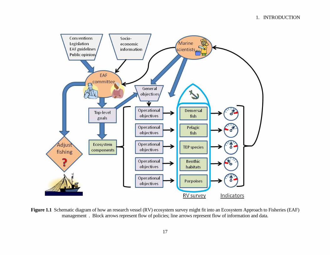
1. INTRODUCTION

17

Figure 1.1 Schematic diagram of how an research vessel (RV) ecosystem survey might fit into an Ecosystem Approach to Fisheries (EAF)

management . Block arrows represent flow of policies; line arrows represent flow of information and data.

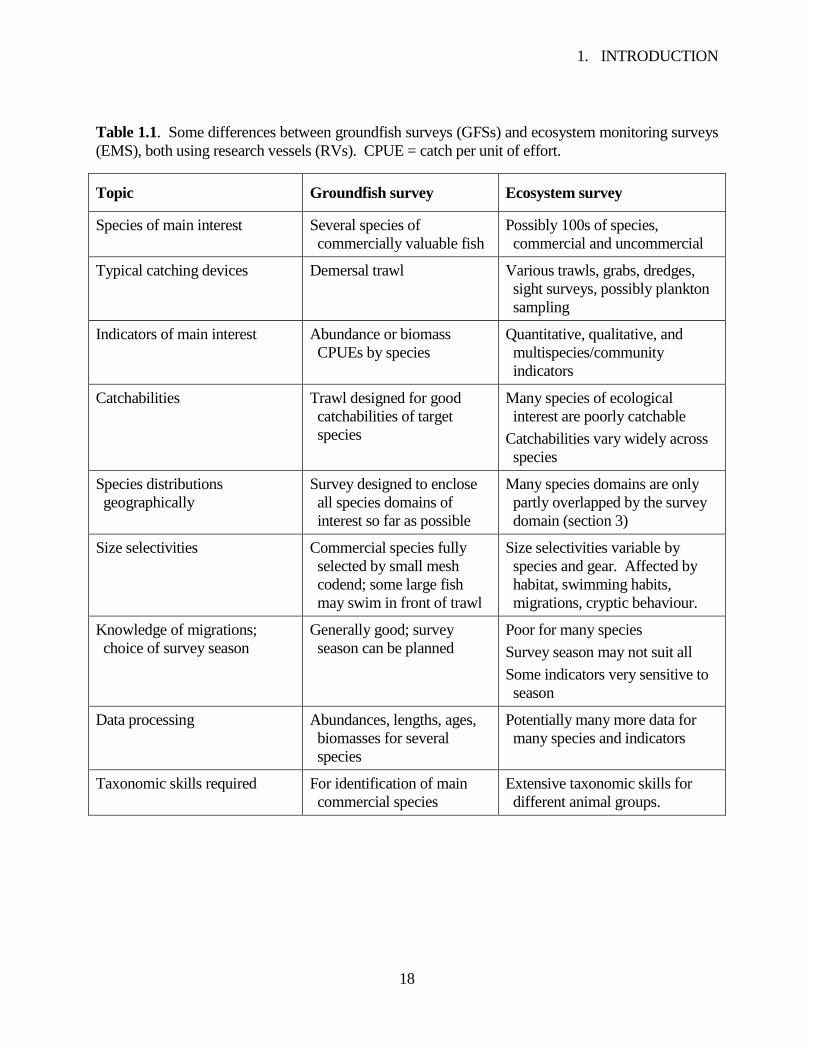
1. INTRODUCTION

18

Table 1.1. Some differences between groundfish surveys (GFSs) and ecosystem monitoring surveys

(EMS), both using research vessels (RVs). CPUE = catch per unit of effort.

Topic Groundfish survey Ecosystem survey

Species of main interest Several species of

commercially valuable fish

Possibly 100s of species,

commercial and uncommercial

Typical catching devices Demersal trawl Various trawls, grabs, dredges,

sight surveys, possibly plankton

sampling

Indicators of main interest Abundance or biomass

CPUEs by species

Quantitative, qualitative, and

multispecies/community

indicators

Catchabilities Trawl designed for good

catchabilities of target

species

Many species of ecological

interest are poorly catchable

Catchabilities vary widely across

species

Species distributions

geographically

Survey designed to enclose

all species domains of

interest so far as possible

Many species domains are only

partly overlapped by the survey

domain (section 3)

Size selectivities Commercial species fully

selected by small mesh

codend; some large fish

may swim in front of trawl

Size selectivities variable by

species and gear. Affected by

habitat, swimming habits,

migrations, cryptic behaviour.

Knowledge of migrations;

choice of survey season

Generally good; survey

season can be planned

Poor for many species

Survey season may not suit all

Some indicators very sensitive to

season

Data processing Abundances, lengths, ages,

biomasses for several

species

Potentially many more data for

many species and indicators

Taxonomic skills required For identification of main

commercial species

Extensive taxonomic skills for

different animal groups.

2. PLANNING AN RV SURVEY

19

2 PLANNING AN RV ECOSYSTEM MONITORING SURVEY (EMS)

Several interlinked tasks must be attended to in advance of an ecosystem monitoring survey

(EMS) to be carried out by an RV. Some of the more important are listed and discussed in this

section. Figure 2.1 summarizes schematically how initial planning of an EMS might proceed.

Different ecosystem measures call for different sampling devices, different RV facilities, and

different sampling domains5. It is important, therefore, to plan the survey so that objectives chosen

for it will be matched to the available resources.

5 „Sampling domain‟ refers to the region and season of sampling.

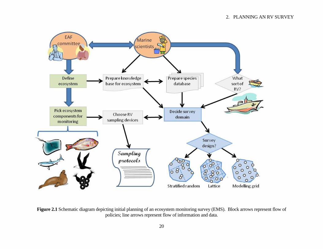
2. PLANNING AN RV SURVEY

20

Figure 2.1 Schematic diagram depicting initial planning of an ecosystem monitoring survey (EMS). Block arrows represent flow of

policies; line arrows represent flow of information and data.

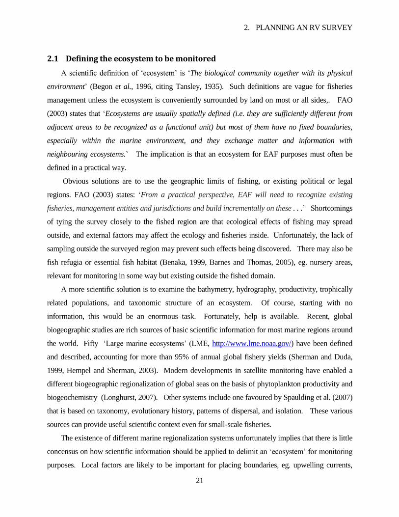
2. PLANNING AN RV SURVEY

21

2.1 Defining the ecosystem to be monitored

A scientific definition of „ecosystem‟ is „The biological community together with its physical

environment‟ (Begon et al., 1996, citing Tansley, 1935). Such definitions are vague for fisheries

management unless the ecosystem is conveniently surrounded by land on most or all sides,. FAO

(2003) states that „Ecosystems are usually spatially defined (i.e. they are sufficiently different from

adjacent areas to be recognized as a functional unit) but most of them have no fixed boundaries,

especially within the marine environment, and they exchange matter and information with

neighbouring ecosystems.‟ The implication is that an ecosystem for EAF purposes must often be

defined in a practical way.

Obvious solutions are to use the geographic limits of fishing, or existing political or legal

regions. FAO (2003) states: „From a practical perspective, EAF will need to recognize existing

fisheries, management entities and jurisdictions and build incrementally on these . . .‟ Shortcomings

of tying the survey closely to the fished region are that ecological effects of fishing may spread

outside, and external factors may affect the ecology and fisheries inside. Unfortunately, the lack of

sampling outside the surveyed region may prevent such effects being discovered. There may also be

fish refugia or essential fish habitat (Benaka, 1999, Barnes and Thomas, 2005), eg. nursery areas,

relevant for monitoring in some way but existing outside the fished domain.

A more scientific solution is to examine the bathymetry, hydrography, productivity, trophically

related populations, and taxonomic structure of an ecosystem. Of course, starting with no

information, this would be an enormous task. Fortunately, help is available. Recent, global

biogeographic studies are rich sources of basic scientific information for most marine regions around

the world. Fifty „Large marine ecosystems‟ (LME, http://www.lme.noaa.gov/) have been defined

and described, accounting for more than 95% of annual global fishery yields (Sherman and Duda,

1999, Hempel and Sherman, 2003). Modern developments in satellite monitoring have enabled a

different biogeographic regionalization of global seas on the basis of phytoplankton productivity and

biogeochemistry (Longhurst, 2007). Other systems include one favoured by Spaulding et al. (2007)

that is based on taxonomy, evolutionary history, patterns of dispersal, and isolation. These various

sources can provide useful scientific context even for small-scale fisheries.

The existence of different marine regionalization systems unfortunately implies that there is little

concensus on how scientific information should be applied to delimit an „ecosystem‟ for monitoring

purposes. Local factors are likely to be important for placing boundaries, eg. upwelling currents,

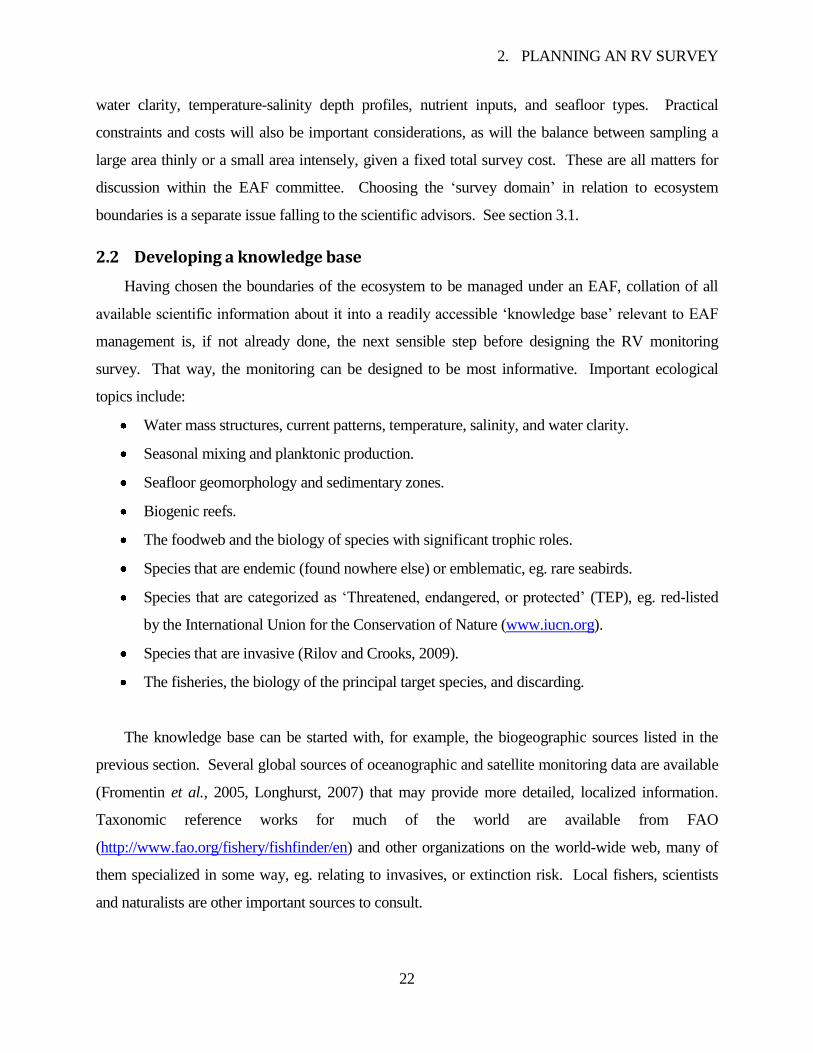
2. PLANNING AN RV SURVEY

22

water clarity, temperature-salinity depth profiles, nutrient inputs, and seafloor types. Practical

constraints and costs will also be important considerations, as will the balance between sampling a

large area thinly or a small area intensely, given a fixed total survey cost. These are all matters for

discussion within the EAF committee. Choosing the „survey domain‟ in relation to ecosystem

boundaries is a separate issue falling to the scientific advisors. See section 3.1.

2.2 Developing a knowledge base

Having chosen the boundaries of the ecosystem to be managed under an EAF, collation of all

available scientific information about it into a readily accessible „knowledge base‟ relevant to EAF

management is, if not already done, the next sensible step before designing the RV monitoring

survey. That way, the monitoring can be designed to be most informative. Important ecological

topics include:

Water mass structures, current patterns, temperature, salinity, and water clarity.

Seasonal mixing and planktonic production.

Seafloor geomorphology and sedimentary zones.

Biogenic reefs.

The foodweb and the biology of species with significant trophic roles.

Species that are endemic (found nowhere else) or emblematic, eg. rare seabirds.

Species that are categorized as „Threatened, endangered, or protected‟ (TEP), eg. red-listed

by the International Union for the Conservation of Nature (www.iucn.org).

Species that are invasive (Rilov and Crooks, 2009).

The fisheries, the biology of the principal target species, and discarding.

The knowledge base can be started with, for example, the biogeographic sources listed in the

previous section. Several global sources of oceanographic and satellite monitoring data are available

(Fromentin et al., 2005, Longhurst, 2007) that may provide more detailed, localized information.

Taxonomic reference works for much of the world are available from FAO

(http://www.fao.org/fishery/fishfinder/en) and other organizations on the world-wide web, many of

them specialized in some way, eg. relating to invasives, or extinction risk. Local fishers, scientists

and naturalists are other important sources to consult.

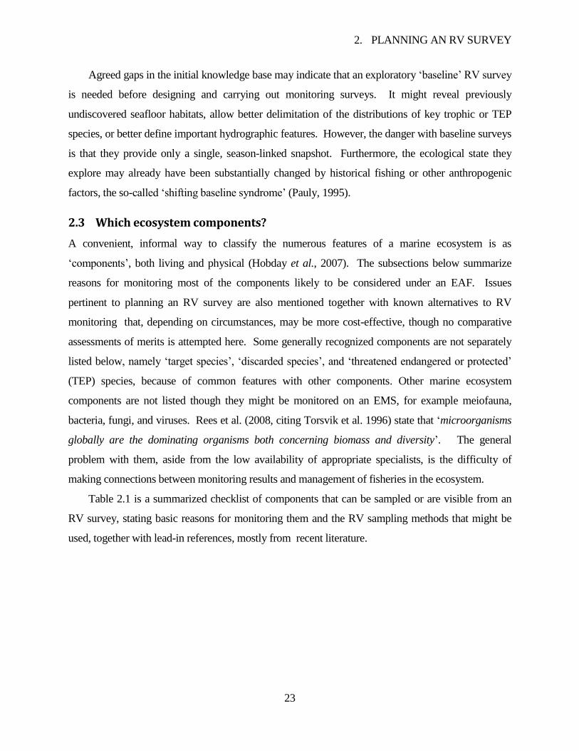
2. PLANNING AN RV SURVEY

23

Agreed gaps in the initial knowledge base may indicate that an exploratory „baseline‟ RV survey

is needed before designing and carrying out monitoring surveys. It might reveal previously

undiscovered seafloor habitats, allow better delimitation of the distributions of key trophic or TEP

species, or better define important hydrographic features. However, the danger with baseline surveys

is that they provide only a single, season-linked snapshot. Furthermore, the ecological state they

explore may already have been substantially changed by historical fishing or other anthropogenic

factors, the so-called „shifting baseline syndrome‟ (Pauly, 1995).

2.3 Which ecosystem components?

A convenient, informal way to classify the numerous features of a marine ecosystem is as

„components‟, both living and physical (Hobday et al., 2007). The subsections below summarize

reasons for monitoring most of the components likely to be considered under an EAF. Issues

pertinent to planning an RV survey are also mentioned together with known alternatives to RV

monitoring that, depending on circumstances, may be more cost-effective, though no comparative

assessments of merits is attempted here. Some generally recognized components are not separately

listed below, namely „target species‟, „discarded species‟, and „threatened endangered or protected‟

(TEP) species, because of common features with other components. Other marine ecosystem

components are not listed though they might be monitored on an EMS, for example meiofauna,

bacteria, fungi, and viruses. Rees et al. (2008, citing Torsvik et al. 1996) state that „microorganisms

globally are the dominating organisms both concerning biomass and diversity‟. The general

problem with them, aside from the low availability of appropriate specialists, is the difficulty of

making connections between monitoring results and management of fisheries in the ecosystem.

Table 2.1 is a summarized checklist of components that can be sampled or are visible from an

RV survey, stating basic reasons for monitoring them and the RV sampling methods that might be

used, together with lead-in references, mostly from recent literature.

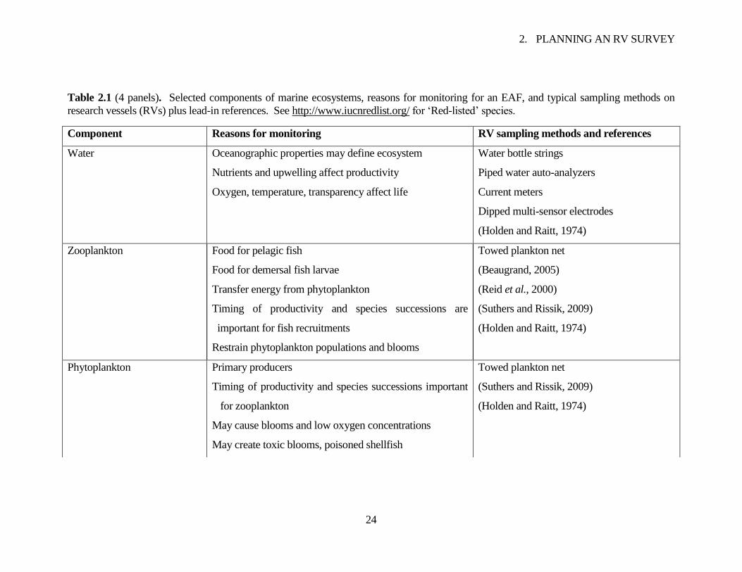
2. PLANNING AN RV SURVEY

24

Table 2.1 (4 panels). Selected components of marine ecosystems, reasons for monitoring for an EAF, and typical sampling methods on

research vessels (RVs) plus lead-in references. See http://www.iucnredlist.org/ for „Red-listed‟ species.

Component Reasons for monitoring RV sampling methods and references

Water Oceanographic properties may define ecosystem

Nutrients and upwelling affect productivity

Oxygen, temperature, transparency affect life

Water bottle strings

Piped water auto-analyzers

Current meters

Dipped multi-sensor electrodes

(Holden and Raitt, 1974)

Zooplankton Food for pelagic fish

Food for demersal fish larvae

Transfer energy from phytoplankton

Timing of productivity and species successions are

important for fish recruitments

Restrain phytoplankton populations and blooms

Towed plankton net

(Beaugrand, 2005)

(Reid et al., 2000)

(Suthers and Rissik, 2009)

(Holden and Raitt, 1974)

Phytoplankton Primary producers

Timing of productivity and species successions important

for zooplankton

May cause blooms and low oxygen concentrations

May create toxic blooms, poisoned shellfish

Towed plankton net

(Suthers and Rissik, 2009)

(Holden and Raitt, 1974)

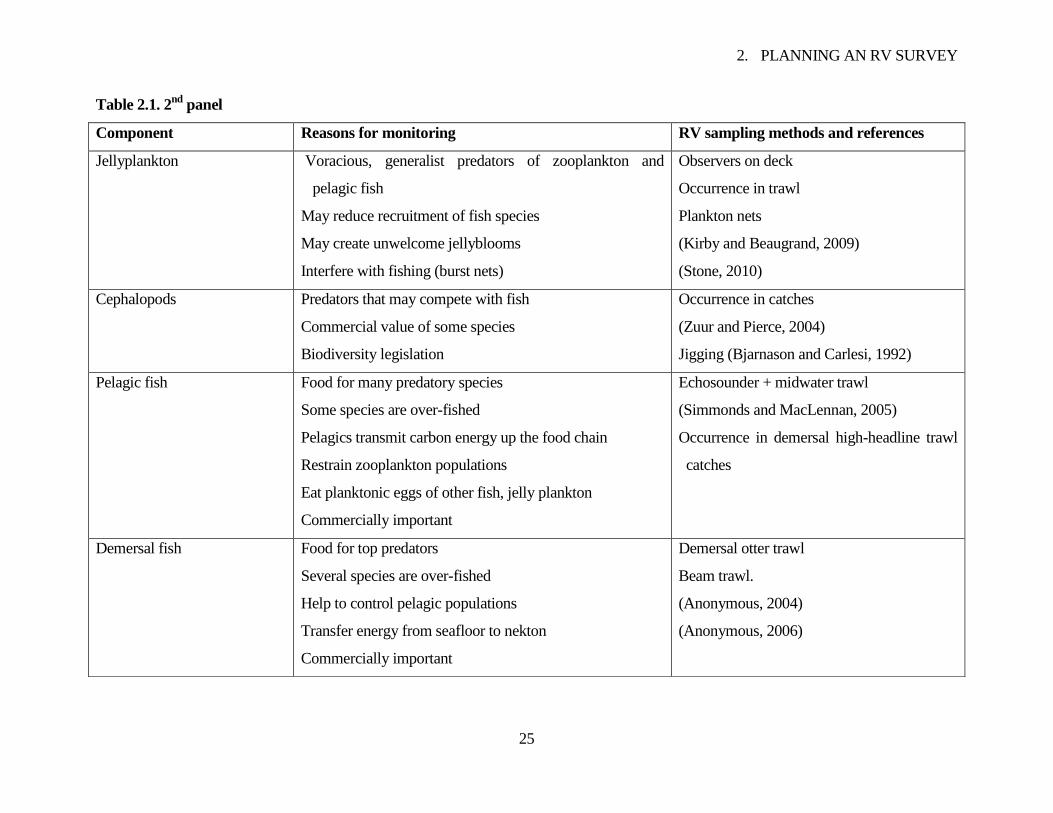
2. PLANNING AN RV SURVEY

25

Table 2.1. 2nd

panel

Component Reasons for monitoring RV sampling methods and references

Jellyplankton Voracious, generalist predators of zooplankton and

pelagic fish

May reduce recruitment of fish species

May create unwelcome jellyblooms

Interfere with fishing (burst nets)

Observers on deck

Occurrence in trawl

Plankton nets

(Kirby and Beaugrand, 2009)

(Stone, 2010)

Cephalopods Predators that may compete with fish

Commercial value of some species

Biodiversity legislation

Occurrence in catches

(Zuur and Pierce, 2004)

Jigging (Bjarnason and Carlesi, 1992)

Pelagic fish Food for many predatory species

Some species are over-fished

Pelagics transmit carbon energy up the food chain

Restrain zooplankton populations

Eat planktonic eggs of other fish, jelly plankton

Commercially important

Echosounder + midwater trawl

(Simmonds and MacLennan, 2005)

Occurrence in demersal high-headline trawl

catches

Demersal fish Food for top predators

Several species are over-fished

Help to control pelagic populations

Transfer energy from seafloor to nekton

Commercially important

Demersal otter trawl

Beam trawl.

(Anonymous, 2004)

(Anonymous, 2006)

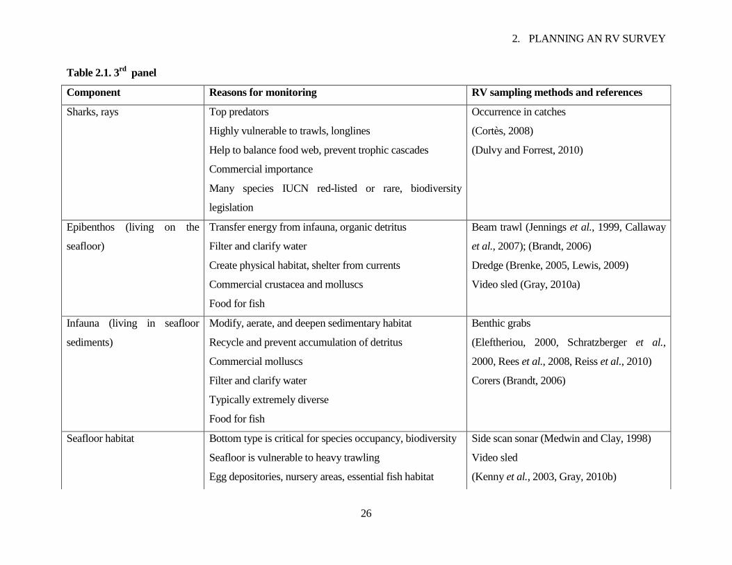
2. PLANNING AN RV SURVEY

26

Table 2.1. 3rd

panel

Component Reasons for monitoring RV sampling methods and references

Sharks, rays Top predators

Highly vulnerable to trawls, longlines

Help to balance food web, prevent trophic cascades

Commercial importance

Many species IUCN red-listed or rare, biodiversity

legislation

Occurrence in catches

(Cortès, 2008)

(Dulvy and Forrest, 2010)

Epibenthos (living on the

seafloor)

Transfer energy from infauna, organic detritus

Filter and clarify water

Create physical habitat, shelter from currents

Commercial crustacea and molluscs

Food for fish

Beam trawl (Jennings et al., 1999, Callaway

et al., 2007); (Brandt, 2006)

Dredge (Brenke, 2005, Lewis, 2009)

Video sled (Gray, 2010a)

Infauna (living in seafloor

sediments)

Modify, aerate, and deepen sedimentary habitat

Recycle and prevent accumulation of detritus

Commercial molluscs

Filter and clarify water

Typically extremely diverse

Food for fish

Benthic grabs

(Eleftheriou, 2000, Schratzberger et al.,

2000, Rees et al., 2008, Reiss et al., 2010)

Corers (Brandt, 2006)

Seafloor habitat Bottom type is critical for species occupancy, biodiversity

Seafloor is vulnerable to heavy trawling

Egg depositories, nursery areas, essential fish habitat

Side scan sonar (Medwin and Clay, 1998)

Video sled

(Kenny et al., 2003, Gray, 2010b)

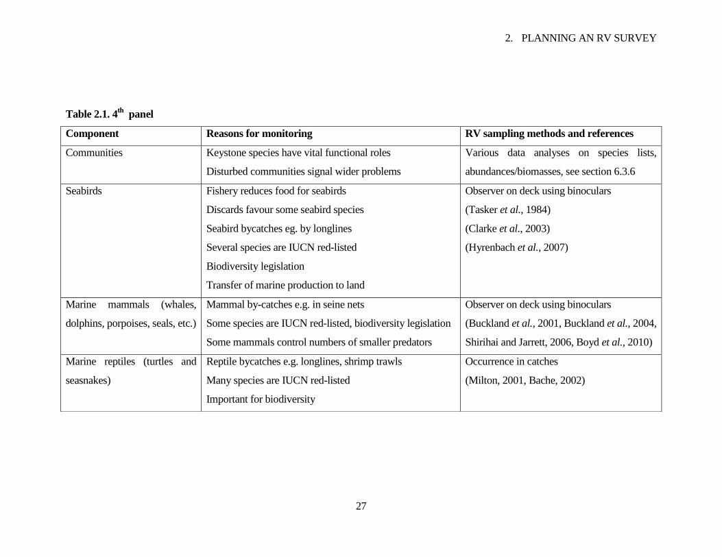
2. PLANNING AN RV SURVEY

27

Table 2.1. 4th

panel

Component Reasons for monitoring RV sampling methods and references

Communities Keystone species have vital functional roles

Disturbed communities signal wider problems

Various data analyses on species lists,

abundances/biomasses, see section 6.3.6

Seabirds Fishery reduces food for seabirds

Discards favour some seabird species

Seabird bycatches eg. by longlines

Several species are IUCN red-listed

Biodiversity legislation

Transfer of marine production to land

Observer on deck using binoculars

(Tasker et al., 1984)

(Clarke et al., 2003)

(Hyrenbach et al., 2007)

Marine mammals (whales,

dolphins, porpoises, seals, etc.)

Mammal by-catches e.g. in seine nets

Some species are IUCN red-listed, biodiversity legislation

Some mammals control numbers of smaller predators

Observer on deck using binoculars

(Buckland et al., 2001, Buckland et al., 2004,

Shirihai and Jarrett, 2006, Boyd et al., 2010)

Marine reptiles (turtles and

seasnakes)

Reptile bycatches e.g. longlines, shrimp trawls

Many species are IUCN red-listed

Important for biodiversity

Occurrence in catches

(Milton, 2001, Bache, 2002)

2. PLANNING AN RV SURVEY

28

2.3.1 Seawater

Many marine ecosystems are best defined for EAF purposes in oceanographic terms. For

example, a zone of nutrient enrichment caused by upwelling of sub-surface waters is likely to support

a rich fishery within that zone, and fronts may cause localized accumulation of food and predators.

Oceanographic currents and water densities can also affect migrations and seasonal refugia of some

fish species. Low oxygen levels or salinities may be avoided by adult fish, and may kill fish larvae.

Transparency is another important feature of seawater. Too much turbidity or plankton reduces light

transmission for primary production and may impair visual hunting by some species. For these and

other reasons, an understanding of the oceanographic features of an ecosystem is important for an

EAF.

Whether or not oceanography should form part of an RV survey will depend on the nature of the

ecosystem and the amount of RV time available. If the oceanography shows consistent patterns from

year to year and is already quite well understood from past monitoring, occasional localized new

sampling by an RV may not add much unless it is part of a wider, co-ordinated programme. Equally,

if the oceanography is highly variable, eg. seasonally, results from the short period of an annual RV

survey will provide little information about seasonal patterns and processes. On the other hand, RV

surveys, preferably multi-seasonal, may be able to fill significant gaps in oceanographic

understanding of some ecosystems by sampling at appropriate times and localities. RVs fitted with

piped water systems feeding automatic analysers on board can sample large amounts of surface-

water easily as they steam around the ecosystem. Sampling underlying water masses is carried out

by lowering strings of water bottles at each station. Multi-sensor electronic devices can be lowered

instead to reduce times on-station but they may not be as accurate or as reliable.

Autonomous and remotely operated underwater vehicles (AUVs and ROVs) can be used to

collect oceanographic data instead, or in support, of an RV. See also the World Ocean Atlas at

http://www.nodc.noaa.gov/OC5/WOA09/pr_woa09.html.

2.3.2 Zooplankton and phytoplankton

Zooplankton play a crucial role in harvesting primary production by phytoplankton and thus

making it available to the rest of the food web. They also control blooms of phytoplankton when

nutrients and light are not limiting primary production. Production and succession of species of both

of these components vary with climate, season, hydrography, light penetration, mixing and nutrients.

Depending on season, zooplankton include the eggs and larvae of pelagically distributed fish,

2. PLANNING AN RV SURVEY

29

planktonic, and benthic species (Rees et al., 2008). According to one writer, „Ongoing plankton

monitoring programmes worldwide will act as sentinels to identify future changes in marine

ecosystems‟ (Hays et al., 2006). Sampling from RVs is usually with towed plankton nets, the

samples being preserved for later analysis in a laboratory under a microscope. The time and

taxonomic skills, and hence costs, required for analysis increase inversely with the mesh size of the

plankton net. Quantitative interpretation of plankton sampling results can be problematic because of

patchy distributions in the sea, diurnal vertical migrations, short life cycles, seasonal successions of

species, variable sinking rates, and the fact that the standing crop is not necessarily related to the rate

of production if that production is being rapidly consumed by planktivores.

Sources of information about plankton that are not dependent on an RV include remote sensing

of chlorophyll concentrations using satellite images (Longhurst, 2007), and the continuous plankton

recorder (CPR) towed behind ships of opportunity (Batten et al., 2003). A recent text on plankton

ecology and processes is by Kiorboe (2008).

2.3.3 Jellyplankton

„Jellyplankton‟ includes ctenophores and jellyfish. Environmental concern about them is quite

recent (Lynam et al., 2006, Richardson et al., 2009). They are unselective consumers of zooplankton

and sometimes fish, possibly showing well-developed foraging behaviour (Hays et al., 2011), yet

they have relatively few predators themselves. Large increases in populations can rapidly occur when

prey is released by reduction of fish predators through fishing. A warming climate and eutrophication

may also favour production of jellyplankton (Richardson et al., 2009). The main concerns about

large populations are that they compete effectively with fish for planktonic food, as well as

consuming large numbers of fish eggs. A marine ecosystem that has become dominated by

jellyplankton might therefore be unlikely to turn back quickly to a fish-dominated state.

Jellyplankton have been reported as concerns for many seas, eg. the Benguela system west of

southern Africa (Lynam et al., 2006), the Baltic (Haslob et al., 2007), the Black Sea (Daskalov,

2008), and the Yellow and Japan Seas (Stone, 2010). Monitoring methods for jellyfish using RVs

may include acoustic systems, observations from an observer platform (Bastian et al., 2011) and,

possibly, occurrences in trawls and plankton nets. Jellyfish CPUE data from trawls are likely to

have high variance because of shoaling, as for pelagic fish (section 2.3.5). Cleaning a trawl of

jellyfish, as is essential after every haul if occurrences or CPUEs are to be collected, requires much

time and labour. Jellyfish can also be monitored from low-flying aircraft (Houghton et al., 2006).

2. PLANNING AN RV SURVEY

30

2.3.4 Cephalopods

Cephalopods such as cuttlefish, squid and octopus may exist in competition with some fish

species so population sizes may respond to changing commercial fishing effort. Cephalopods are

sometimes targeted by fishers when other stocks are low. Jigging using lights to attract to the vessel

is a common fishing technique for squid (Bjarnason and Carlesi, 1992). Some species are quite

resilient to heavy fishing because of an annual life cycle. Species occurring in catches of an RV

survey trawl should be recorded, but soft-bodied forms are likely to be damaged by trawl nets and

difficult to process beyond simple counting. Also, size distributions found in nets often differ

substantially from sizes found in the stomach contents of predators (Boyle and Rodhouse, 2005)

implying that length distributions obtained on an RV are likely to be biased anyway. Populations of

pelagic cephalopods can be assessed acoustically (Goss et al., 2001). An alternative to an RV for

monitoring cephalopods is to use catch data from observer surveys on commercial fishing boats,

preferably jiggers to minimise damage to the catch.

2.3.5 Pelagic fish

In some parts of the world, pelagic fish are caught in large quantities by industrial-scale fishing

fleets. This can impede the passage of primary production biomass to higher trophic levels, as in so-

called „wasp-waist‟ ecosystems (Cury et al., 2000, Smith et al., 2011). As a result, fisheries on

valuable predatory species show lower yields, and seabird populations may be affected. Another

consequence of reduced populations of pelagic species may be over-production of their

zooplanktonic prey leading, in turn, to expansion of populations of ctenophores or other jellyplankton

„thriving on the food no longer consumed by fish‟ (Lynam et al., 2006). See the „Jellyfish‟

component (section 2.3.3). On the other hand, increased populations of certain pelagics may cause

excessive predation of planktonic fish eggs, leading to poor recruitment and impeded recovery of

predatory species, eg. sprat eating the eggs of cod in the Baltic (Casini et al., 2008). Pelagic species

can be monitored acoustically from an RV with regular tows of a pelagic trawl to confirm the identity

of species found with the echosounder (MacLennan and Simmonds, 2010). Egg-production surveys

(Stratoudakis et al., 2006) are a second RV monitoring method for some pelagic stocks. They

estimate the size of the adult stock from concentrations of planktonic eggs, spawning patterns, and

fecundities. A third RV monitoring method for pelagic species swimming near the seafloor – as

some do during the day – uses a high-headline demersal otter trawl. However, average catch per unit

effort (CPUE) indicators for shoaling adults of pelagic species are seldom reliable because extreme

2. PLANNING AN RV SURVEY

31

results are common:- the trawl either catches very large numbers if the tow clips a shoal, or virtually

none if it misses it altogether. Better may be to record „shoal present‟ or „shoal absent‟ using an

arbitrary threshold number of fish to signify a shoal, and to analyse as occupancies (section 5.1.1).

Trawling may be best timed and located so as to catch young fish before they aggregate as shoals.

Recent articles on pelagic species, including RV survey methods, can be found in Checkley et al

(2009) for example.

As alternatives to using an RV, stocks of pelagic species can be assessed from commercial

landings statistics, or possibly from data collected by observers on commercial fishing vessels

combined with automatic vessel monitoring systems (VMS). Aerial fish spotting has been used in

California and Namibia.

2.3.6 Demersal fish

Demersal fish are categorized informally as round- or flatfish according to body shape. They

form the principal targets of many commercial trawling and netting fisheries. As predators, demersal

fish serve an important trophic role by helping to restrict population sizes of prey species, and by

routing food energy from low trophic levels to higher predators such as marine mammals and sharks.

Demersal species often change their feeding habits and trophic level as they get older and larger

(Jennings et al., 2002a). Roundfish tend to live on or near the seafloor, though they may rise up at

night in step with vertical migrations of their prey. They tend to be best caught by an RV during the

day using an otter trawl because of the wide towing path and the herding effects of otter boards and

sweeps. Most flatfish, on the other hand, are generally best caught by heavy beamtrawls fitted with

tickler chains to raise them out of the sediment and into the path of the net. The nature of the

seafloor can strongly affect the efficiency of trawling. Trawls with a light footrope make good

ground contact on smooth seafloors but cannot be used where there are rocks. Rockhopper trawls are

fitted with large rollers on the groundrope to deal with rocks but fish can escape between the rollers.

Lining or netting may have to be considered for sampling demersal species in very rocky areas or

reefs. There is a large literature on RV demersal trawl surveys, eg. (Anonymous, 2004, Anonymous,

2006).

Non-RV sources of information on demersal fish are data collected at fish markets or by

observers on commercial fishing vessels, and commercial CPUE data.

2. PLANNING AN RV SURVEY

32

2.3.7 Sharks, skates and rays

Many species of sharks and rays are top predators, serving a similar trophic role as mammalian

top predators. Sharks are particularly vulnerable to longlines if fitted with wire leaders that cannot be

bitten through (Ward et al., 2008). Large pelagic rays are also caught by this method. Some sharks

and many rays are vulnerable to trawls, and some species are dependent on special habitats for

reproduction, feeding, and migrations (Ellis et al., 2008). Many sharks and rays are now being

caught at low rates compared to historically, and several species are probably in danger of extinction

even though, because information is lacking, they are not yet officially on the Red list of the IUCN

(Dulvy and Forrest, 2010). For a summary of various conservation listings, see Ellis et al. (2008). A

survey intended to gain information about sharks might use longlining or fixed nets to obtain

reasonable capture rates, eg. as in the Bay of Bengal (http://goo.gl/6ibrc; http://goo.gl/kqmNO).

Encounter rates for pelagic sharks in RV trawls are likely to be low, yielding little quantitative

information. However, demersal skate and ray species are regularly caught by demersal trawls when

present and could be monitored, as for fish, by trawling from an RV. For recent articles on the

biology and ecology of sharks and their relatives, see Hamlett (1999) and Carrier et al. (2010).

Monitoring of sharks, skates and rays without using an RV can be carried out at fish markets and

by observers on commercial fishing vessels, particularly longliners. Large surface-visiting sharks

such as basking sharks can be surveyed aerially. Archival tagging is another option for studying

these animals (Metcalfe et al., 2008).

2.3.8 Epibenthos

Epibenthos are the animals living on the seafloor. Those living attached to the seafloor

contribute to the micro-environment of the seafloor habitat („biogenic‟) and are probably best

monitored as part of a habitat component (Hobday et al., 2007); see section 2.3.10. Those that are

mobile form a trophic bridge between infauna and demersal species. They can also affect benthic

ecological recruitment and restrict the succession of species by predation on settling larvae.

Planktonic larvae of epibenthic species – which may arise in great numbers at certain seasons –

compete with holoplanktonic species such as copepods (Lindley et al., 1995) thereby changing

planktonic communities and perhaps affecting development of fish larvae. Several epibenthic

species have direct economic importance, e.g. crabs, lobsters, mussels.

Epifauna can be monitored using the main survey trawl intended to catch demersal fish.

However, otter trawls, depending on ground gear and mesh sizes, tend to catch only small amounts

2. PLANNING AN RV SURVEY

33

of epibenthos. Beam trawls can take large amounts but the large meshes in the belly of commercial

beam trawls may mean that catchabilities for some epibenthic species are low. A good solution on

an RV survey, if feasible, is to make supplementary tows with a specially designed epibenthic trawl

or dredge. See section 2.5.4. Trials may be needed to find the best design for local conditions.

Whatever gear is used by an RV, catches of epifauna are likely to be strongly affected by the recent

history of commercial trawling in the area.

2.3.9 Infauna

The infauna are a highly diverse group of species that live in the sediment of the seafloor, for

example annelid worms, bivalve molluscs, and many other invertebrate phyla. Many species feed on

organic detritus by filtering the water. The resulting clearer water can, itself, be important for other

species (Breitburg and Riedel, 2005). Other infaunal species can digest organic matter from

sediments and thus re-introduce food into the macro-ecological food web. Infaunal species

contribute planktonic larvae that serve as food for other plankton and fish larvae (Rees et al., 2008).

Several infaunal species form burrows and, by moving water through them, aerate the sediments and

permit aerobic life forms to live at greater depths in the sediment, thereby adding to the organic

matter recycled to the water column from the bottom sediments. Deep-burrowing infaunal forms

assist these processes by exchanging deep and shallow sediments. Benthic communities have been

used as indicators of trawling pressure (Hiddink et al., 2006b).

Monitoring of infauna on RV surveys is usually done with a benthic grab or corer that takes a

bite of sediment at each location. The RV is not held up for a long time, but the infaunal samples

take much time and skill to process because of the high variability between samples and the

difficulties of identifying the many species typically found. Standardized sieving of the sediments is

essential since more and more species can be found as mesh sizes decrease. Difficulties of

identification also tend to increase inversely with size.

2.3.10 Seafloor habitats

Hobday et al. (2007) proposed classifying seafloor habitats according to three variables:

substrate type, geomorphology, and structural fauna. Each of these can be further subdivided into

standard categories that are relevant to the types of species living there. Simple keyword descriptors

are listed in Table 2.2, Table 2.3, andTable 2.4. Examples of seafloor habitats are soft mudbanks,

gravel covered by structural epifauna, rocky outcrops, and cold- and warm-water reefs. Physically

structured benthic habitats are important as nursery and feeding areas, for laying eggs (e.g. herring),

2. PLANNING AN RV SURVEY

34

for protection from predators, and for biodiversity. Different types of habitat have different

vulnerabilities to fishing gear, most notably to trawls. Removal of seafloor structure, both

topographic and epifaunal, is a significant deleterious effect of trawling leading to less shelter from

strong currents, less sedimentation of detrital food, less shelter from predators, and altered functional

composition (Tillin et al., 2006). For these reasons, seafloor habitats, especially any designated as

marine protected areas (MPAs, http://www.wdpa-marine.org/#/countries/about) (Gubbay, 1995,

Claudet, 2011) or essential fish habitat (EFH, http://www.habitat.noaa.gov/protection/efh/index.html)

(Benaka, 1999) should be monitored as part of an EAF. Epibenthic trawls and dredges provide

partial indications of habitat types if, for example, mud, gravel, or attached fauna are retrieved.

However, they do not reveal the geophysical structure of the habitat. For this, acoustic or video

imaging is necessary (Kenny et al., 2003). Even then, interpretation of changes may be difficult to

link with trawling (Hiddink et al., 2006b) unless trawl tracks can be seen. Ideally, detailed

information on commercial trawling effort between RV surveys will be available. A study of this

type was reported by (Callaway et al., 2002a, Callaway et al., 2007).

Sedimentological and hydrographic information may be available for a marine ecosystem

without special new sampling by an RV if general geological or hydrographic surveys have covered

the area, eg. in relation to mineral extraction or environmental impact assessments for offshore

constructions.

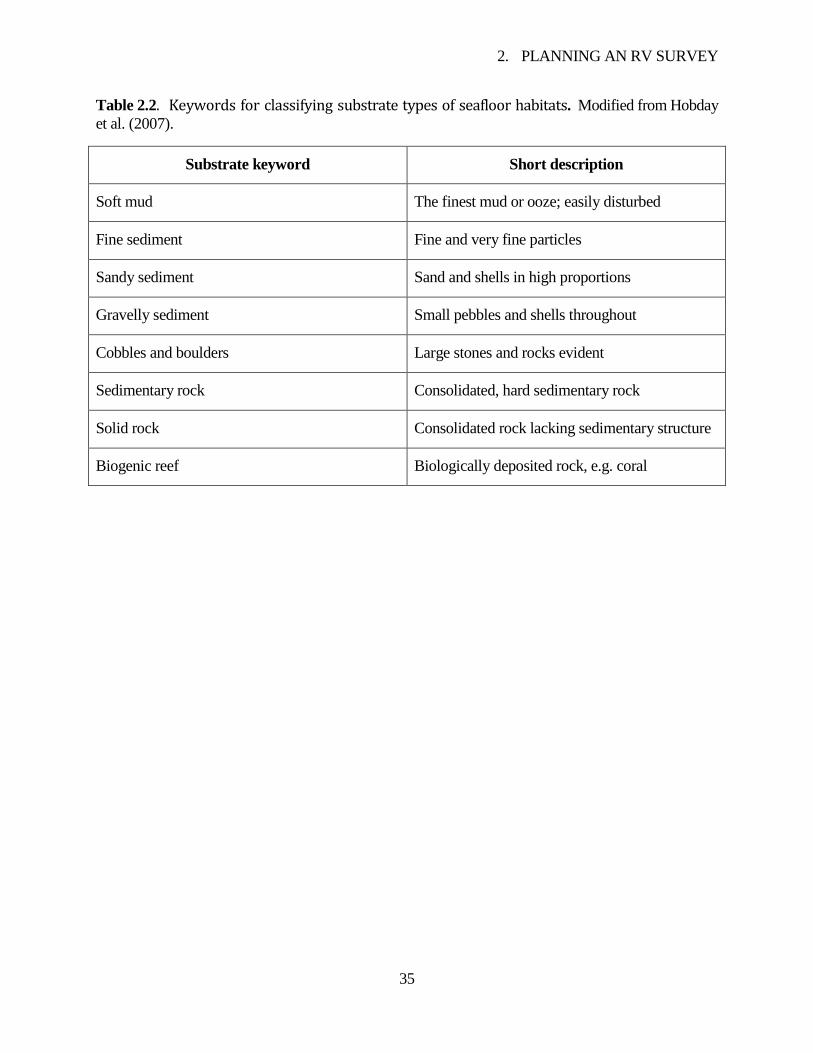
2. PLANNING AN RV SURVEY

35

Table 2.2. Keywords for classifying substrate types of seafloor habitats. Modified from Hobday

et al. (2007).

Substrate keyword Short description

Soft mud The finest mud or ooze; easily disturbed

Fine sediment Fine and very fine particles

Sandy sediment Sand and shells in high proportions

Gravelly sediment Small pebbles and shells throughout

Cobbles and boulders Large stones and rocks evident

Sedimentary rock Consolidated, hard sedimentary rock

Solid rock Consolidated rock lacking sedimentary structure

Biogenic reef Biologically deposited rock, e.g. coral

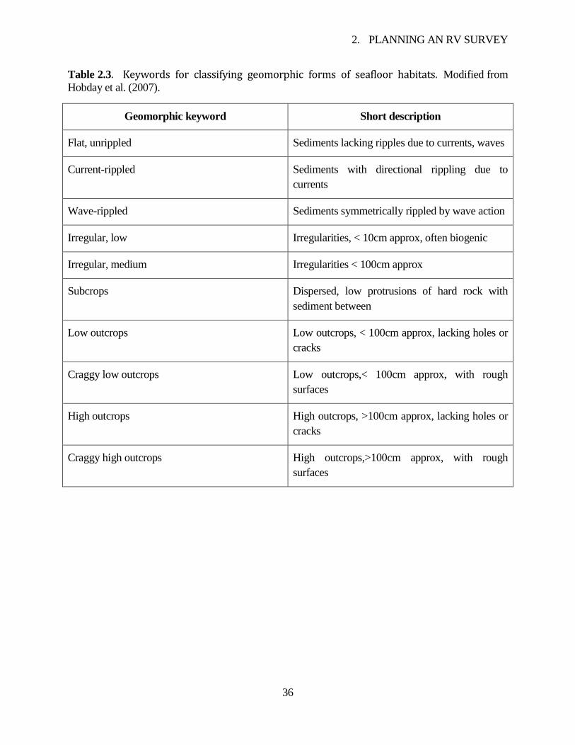
2. PLANNING AN RV SURVEY

36

Table 2.3. Keywords for classifying geomorphic forms of seafloor habitats. Modified from

Hobday et al. (2007).

Geomorphic keyword Short description

Flat, unrippled Sediments lacking ripples due to currents, waves

Current-rippled Sediments with directional rippling due to

currents

Wave-rippled Sediments symmetrically rippled by wave action

Irregular, low Irregularities, < 10cm approx, often biogenic

Irregular, medium Irregularities < 100cm approx

Subcrops Dispersed, low protrusions of hard rock with

sediment between

Low outcrops Low outcrops, < 100cm approx, lacking holes or

cracks

Craggy low outcrops Low outcrops,< 100cm approx, with rough

surfaces

High outcrops High outcrops, >100cm approx, lacking holes or

cracks

Craggy high outcrops High outcrops,>100cm approx, with rough

surfaces

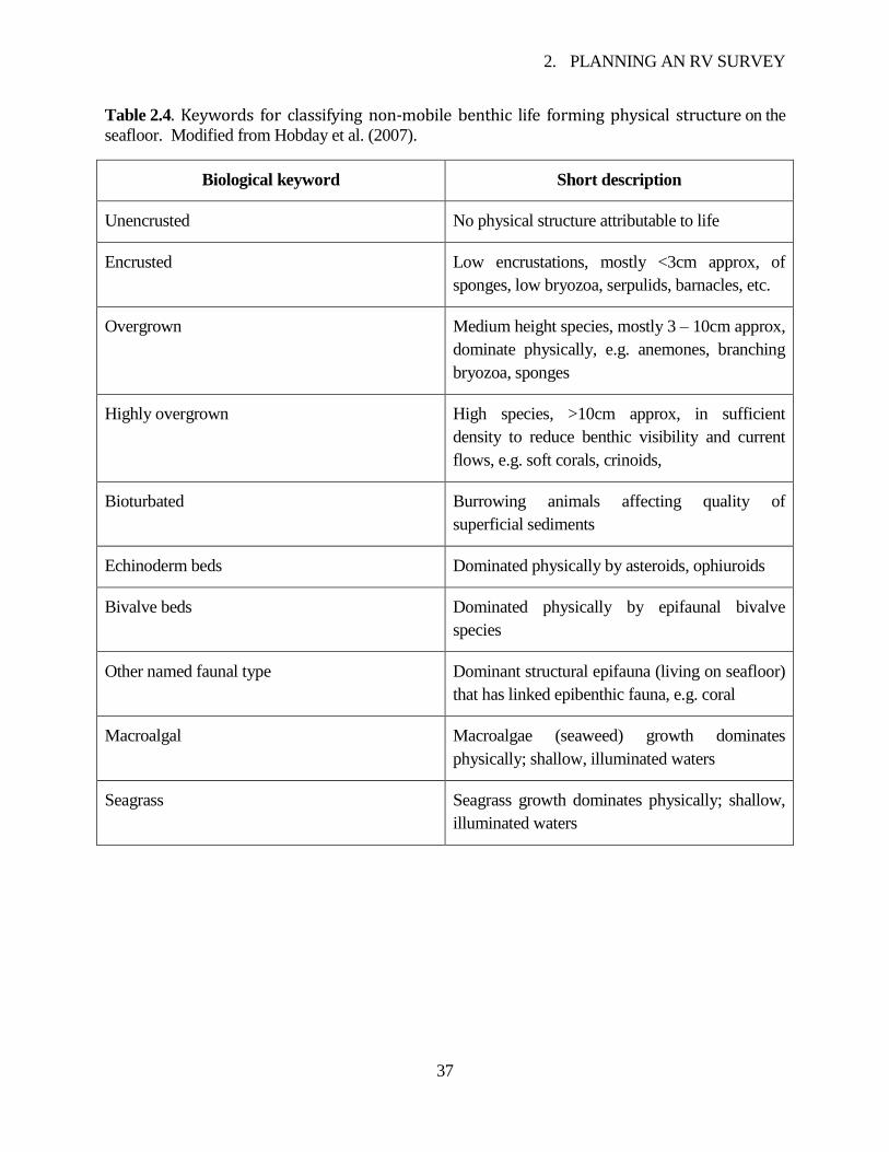
2. PLANNING AN RV SURVEY

37

Table 2.4. Keywords for classifying non-mobile benthic life forming physical structure on the

seafloor. Modified from Hobday et al. (2007).

Biological keyword Short description

Unencrusted No physical structure attributable to life

Encrusted Low encrustations, mostly <3cm approx, of

sponges, low bryozoa, serpulids, barnacles, etc.

Overgrown Medium height species, mostly 3 – 10cm approx,

dominate physically, e.g. anemones, branching

bryozoa, sponges

Highly overgrown High species, >10cm approx, in sufficient

density to reduce benthic visibility and current

flows, e.g. soft corals, crinoids,

Bioturbated Burrowing animals affecting quality of

superficial sediments

Echinoderm beds Dominated physically by asteroids, ophiuroids

Bivalve beds Dominated physically by epifaunal bivalve

species

Other named faunal type Dominant structural epifauna (living on seafloor)

that has linked epibenthic fauna, e.g. coral

Macroalgal Macroalgae (seaweed) growth dominates

physically; shallow, illuminated waters

Seagrass Seagrass growth dominates physically; shallow,

illuminated waters

2. PLANNING AN RV SURVEY

38

2.3.11 Communities

Communities of species are an important component of marine ecosystems in all habitats

because of the vital functional roles of some of the species and their dependence on others. Changes

in the species compositions of species can be gradual and subtle, and neighbouring communities tend

to merge into one another geographically, making them difficult to monitor individually unless there

are marked changes of habitat, e.g. between sediment and rock. Also, communities are naturally

variable with regard to species composition and density of habitation, making the interpretation of

sampling results difficult. For discussion of the difficulties in relation to ecological risk assessment

(PSA method), see Hobday et al. (2007). Communities are sampled and recorded automatically

when species and habitats are identified, counted and, preferably, weighed at RV sampling stations.

For that reason, the monitoring of ecological communities occurs at the data analysis stage and does

not necessarily call for new sampling techniques.

2.3.12 Seabirds

Seabirds are valued aesthetically and as contributors to biodiversity though they are not

numerous in in all marine regions. Many seabird species are declining in number due to loss of

nesting sites, nest raiders such as rats, and food shortages, especially around breeding colonies where

low stocks of surface-swimming pelagic species may prevent adults feeding their chicks. Certain

species are also directly vulnerable to fishing gear, notably when they dive for fish in trawls or on

baited longlines. Many species are known to be nearing extinction (http://www.iucnredlist.org/).

They include most albatrosses, and several shearwaters and petrels (Onley and Scofield, 2007). On

the other hand, some seabird species benefit greatly from galley waste, fish offal, and whole fish

discarded by fishing boats. This leads to a changing balance of seabird species in the ecosystem. See

Schreiber (2001), for example, for articles on biology and ecology. Monitoring of seabirds from RVs

is usually carried out with „sight surveys‟ using specially trained scientific crew with binoculars.

Ships of opportunity may be used instead. Many species can also be monitored by surveys of nesting

sites around breeding times.

2.3.13 Mammals

Many species of marine mammals are top predators. By eating smaller predators, their numbers

are controlled and predation on mid trophic levels is moderated, thereby contributing to healthy

populations of pelagic fish and helping to prevent trophic cascades. Marine mammals are also

important for public interest and for biodiversity. Several species are IUCN red-listed. They can be

2. PLANNING AN RV SURVEY

39

at risk from purse seiners, netters, and fast pair trawlers. On the other hand, seals and other mammals

may compete with fisheries by eating commercial species or their food, or they may damage fish

captured by fixed nets, lines and traps. Marine mammals must come to the sea surface regularly to

breathe, making them visible to watchers on an RV. Monitoring of mammals from RVs is usually

carried out opportunistically by scientists watching seabirds but, in many geographic regions,

encounter rates will be low and little analyzable data will be obtained. Marine mammals can also be

monitored by aerial surveys, shore-based surveys and scat collections at haul-out sites of Pinnipedia

(seals), passive acoustic listening buoys, and archival tagging (Metcalfe et al., 2008). For recent

articles on biology and ecology, see Hoelzel (2002), for example.

2.3.14 Reptiles

Seven species of sea turtle occur in the tropical and temperate waters of the oceans. All are red-

listed by IUCN, mostly in the highest category: „critically endangered‟. This is partly because of

vulnerability to fishing nets and lines but, additionally, turtles suffer from theft of eggs, high

predation on young individuals, and from pollution, eg. by floating plastics mistaken for food. Many

species of seasnakes are found in tropical waters. Although often poisonous to man, they are valued

for biodiversity and probably other ecological roles. They are vulnerable to certain types of fisheries,

notably shrimp trawlers (Milton, 2001). Monitoring of marine reptiles from RV surveys is generally

impractical because of low capture rates and the low, poorly visible profiles of free-living, surfacing

individuals. When caught, reptiles should be released alive if possible after quickly photographing

and measuring. Marine reptiles can sometimes be monitored without using an RV by divers, archival

tagging, or by observer surveys on commercial fishing boats taking them as bycatch. There are

several general texts on biology and ecology (eg. Lutz and Musick, 1996, Spotila, 2004).

2.3.15 Conclusions

An RV survey can feasibly monitor many components of a marine ecosystem including: water,

plankton, jellyplankton, pelagic fish, demersal fish and skates and rays depending on the type of

trawl used, attached and mobile epibenthos, infauna, seafloor habitats, and seabirds. However, this

does not mean that monitoring of all or even most of them on the same RV cruise would be practical.

Components less suited for RV monitoring are ctenophores, cephalopods, pelagic sharks, marine

mammals, sea turtles, and sea snakes. Monitoring of ecological communities, another important

component, can be considered at the data analysis stage provided that results for abundances and

biomasses were collected for all or most species found at each station. Generally, the components

2. PLANNING AN RV SURVEY

40

that can be monitored by RV depend on the gears that can be deployed, the allowable times on

station, the deck space, crew and equipment available and, in some circumstances, whether or not the

survey can be conducted seasonally rather than just annually.

2.4 What sort of research vessel (RV)?

Practical factors that affect the amount of information and types of indicators available from an

RV ecosystem monitoring survey (EMS) include:

The amount of time allowable for sampling at each station

The sampling devices that can be deployed on-station or whilst steaming

The amount of sample processing that can be done on deck or, after the survey, on land

The training and expertise of the scientific sampling crew

The quality of shelter and working conditions for scientists on deck

The weather, and the seaworthiness of the RV

Steaming times between stations, and access by the RV to all parts of the ecosystem

The seasonal timing of the survey.

The size of the RV is relevant to most of these factors. Small RVs are limited to inshore waters

and relatively calm weather, have limited accommodation for scientists, and lack safe deck space and

other facilities for scientific work. Large RVs, on the other hand, cannot access shallow waters, can

work in somewhat worse weather with larger scientific crews, and have more space and facilities for

work on deck and in cabins. Large RVs may be able to steam faster between stations but fuel costs

rise substantially with speed. The high overhead costs of large RVs usually means that they are kept

busy with projects throughout the year. This can restrict their availability for an EMS within the

season preferred for monitoring indicators of reproductive potential and growth, or for sampling

seasonally migrating species. This reasoning warns that a large and expensive RV is not

automatically the best option for an EMS. The different types of RV suitable for an EMS are

discussed in the sub-sections below. Points made are summarized in Table 2.5.

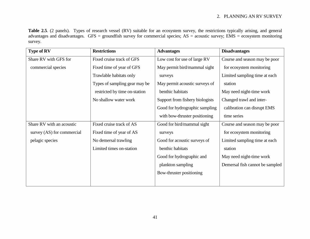
2. PLANNING AN RV SURVEY

41

Table 2.5. (2 panels). Types of research vessel (RV) suitable for an ecosystem survey, the restrictions typically arising, and general

advantages and disadvantages. GFS = groundfish survey for commercial species; AS = acoustic survey; EMS = ecosystem monitoring

survey.

Type of RV Restrictions Advantages Disadvantages

Share RV with GFS for

commercial species

Fixed cruise track of GFS

Fixed time of year of GFS

Trawlable habitats only

Types of sampling gear may be

restricted by time on-station

No shallow water work

Low cost for use of large RV

May permit bird/mammal sight

surveys

May permit acoustic surveys of

benthic habitats

Support from fishery biologists

Good for hydrographic sampling

with bow-thruster positioning

Course and season may be poor

for ecosystem monitoring

Limited sampling time at each

station

May need night-time work

Changed trawl and inter-

calibration can disrupt EMS

time series

Share RV with an acoustic

survey (AS) for commercial

pelagic species

Fixed cruise track of AS

Fixed time of year of AS

No demersal trawling

Limited times on-station

Good for bird/mammal sight

surveys

Good for acoustic surveys of

benthic habitats

Good for hydrographic and

plankton sampling

Bow-thruster positioning

Course and season may be poor

for ecosystem monitoring

Limited sampling time at each

station

May need night-time work

Demersal fish cannot be sampled

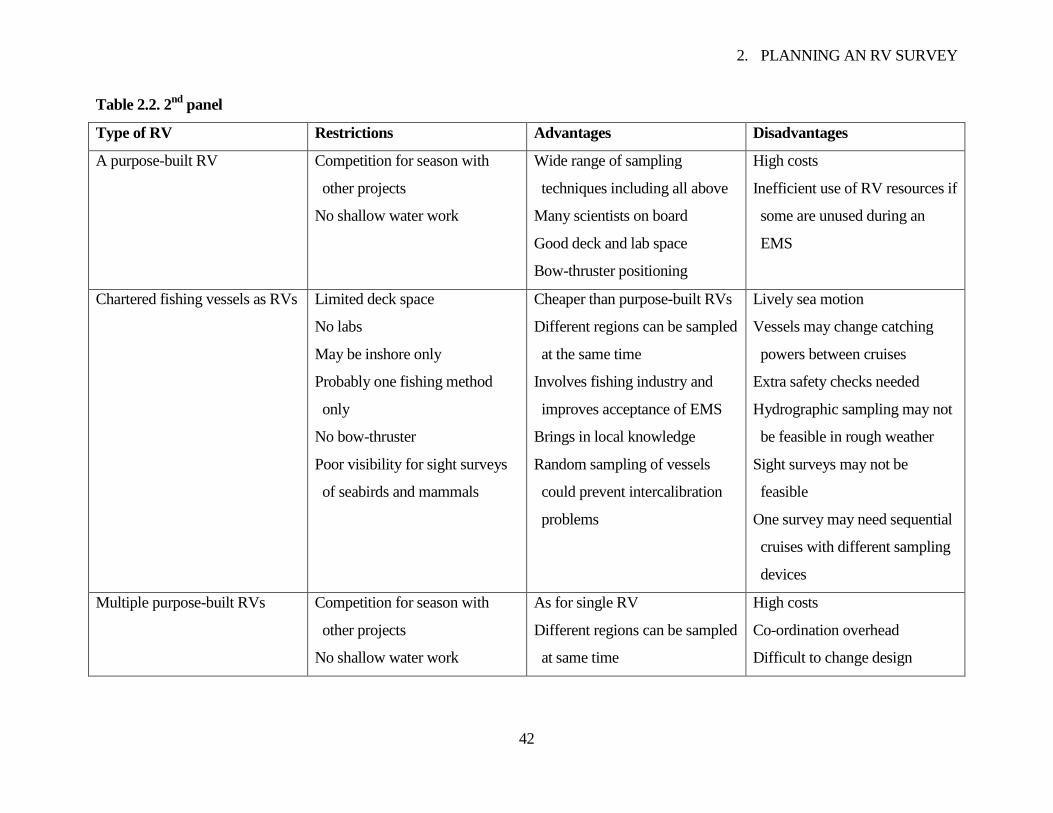
2. PLANNING AN RV SURVEY

42

Table 2.2. 2nd

panel

Type of RV Restrictions Advantages Disadvantages

A purpose-built RV Competition for season with

other projects

No shallow water work

Wide range of sampling

techniques including all above

Many scientists on board

Good deck and lab space

Bow-thruster positioning

High costs

Inefficient use of RV resources if

some are unused during an

EMS

Chartered fishing vessels as RVs Limited deck space

No labs

May be inshore only

Probably one fishing method

only

No bow-thruster

Poor visibility for sight surveys

of seabirds and mammals

Cheaper than purpose-built RVs

Different regions can be sampled

at the same time

Involves fishing industry and

improves acceptance of EMS

Brings in local knowledge

Random sampling of vessels

could prevent intercalibration

problems

Lively sea motion

Vessels may change catching

powers between cruises

Extra safety checks needed

Hydrographic sampling may not

be feasible in rough weather

Sight surveys may not be

feasible

One survey may need sequential

cruises with different sampling

devices

Multiple purpose-built RVs Competition for season with

other projects

No shallow water work

As for single RV

Different regions can be sampled

at same time

High costs

Co-ordination overhead

Difficult to change design

2. PLANNING AN RV SURVEY

43

2.4.1 An RV shared with a groundfish survey (GFS)

Groundfish surveys (GFSs), as mentioned in the Introduction (section 1), are demersal trawl

surveys used to estimate CPUE abundance indices of demersally swimming commercial fish species.

Usually, the codend of the trawl is fitted with a fine-mesh liner intended to catch young fish that will

recruit to the commercial fishery in the coming year or two. Since demersal trawls are poorly

selective for species, many varieties of fish are caught that are likely to be of interest for an EMS.

Additionally, time may be available at each trawl station for sampling with other sampling devices,

depending on the distance to be covered each day and the weather. Other ecosystem monitoring

techniques might be carried out while the RV is steaming between trawl stations, eg. sight surveys

for seabirds and mammals, acoustic surveys of seafloor habitats. A general constraint when using

GFSs is that the cruise track and timing may not be that preferred for ecosystem work.

Fish-related ecosystem indicators derived directly from catches made by the main GFS trawl

include CPUEs, length frequency distributions, and others discussed in section 5.1. However, the

GFS trawl will be specialized for catching commercial species and may catch indicator species

poorly. Frequent occurrences of small numbers of a species in hauls do not necessarily indicate that

that species is highly catchable when present; sporadic catches may just arise because of the large

areas towed over during a GFS. Similarly, an indicator species having the same shape as a

commercial species is not necessarily equally catchable; it may live in a more sheltered habitat, for

example. The effect of poor catchabilities of certain species is to increase the variances of indicators,

as discussed in section 6.1.2.

A well-recognized problem with GFS trawling arises when the RV itself, or the trawl gear, must

be updated or otherwise altered for practical reasons. Catchabilities of different species and size

groups could then be affected, leading to a re-scaling of catch-per-unit-effort (CPUE) indices relative

to species abundances or biomasses. Before-after comparisons, parallel towing, or modelling studies

can be applied to try to intercalibrate the two different RV-gear states (Anonymous, 2006) but, even

in the best of circumstances, the step-change in CPUE time series is difficult and costly to estimate

and may depend on strong assumptions. Intercalibration is a larger problem for EMSs than for GFSs

because more species must be considered. Ecosystem indicators based on CPUEs are not the only

ones affected. Presence-absence rates may also vary with different trawls, particularly for species

that are only marginally catchable. This can lead to step changes in diversity indices, and to

different, possibly spurious, assessments of rarity in biodiversity studies. Size-dependent indicators

2. PLANNING AN RV SURVEY

44

will also be affected by different size-selectivity properties, as will reproductive indicators because

maturation is related to size. For these reasons, the need to intercalibrate a GFS trawl could seriously

disrupt EMS time series. Trawl design for EMSs is discussed under ecosystem sampling techniques

in section 2.5.3.

When deploying ecosystem sampling devices other than the main GFS trawl, speed of working

is important to avoid delaying the vessel unduly. Grabs, corers, and water samplers can be worked

quickly. Long tows of plankton nets or benthic trawls may not be acceptable to a GFS cruise leader,

particularly at deep stations requiring much warp to be paid out and retrieved. Time-consuming

ecosystem sampling methods may, however, be allowed at night if GFS trawling is only carried out

in daylight, as is often the case because of diurnal vertical migrations of many fish species.

However, the RV must be crewed and lit sufficiently for operating the sampling gear safely at night.

2.4.2 An RV shared with an acoustic survey

Acoustic surveys are used to estimate biomass of shoaling commercial pelagic species. The RV

generally zig-zags over the area believed to be occupied by the species recording the strength of

echos received by a calibrated echosounder in order to estimate the number and density of shoals. At

intervals, a midwater trawl must be fished to estimate species compositions. The need to keep the

RV moving on acoustic surveys favours sight surveys for seabirds and mammals but may restrict

times stopped on-station for special ecosystem sampling work, as on GFSs (above). Acoustic

surveys, in Scotland for example, have successfully incorporated hydrographic and plankton

mapping, as well as acoustic seabed classification using single and multi-beam systems. Demersal

trawling is not usually possible on acoustic surveys because of the need to keep using the midwater

trawl.

2.4.3 A purpose-built RV

A vessel purpose-built for scientific work, depending on its cost, is likely to have some or all of

the following facillities for ecosystem monitoring:

Large gantries and winches for different fishing techniques, e.g. otter and beam trawling.

Davits and small winches for other sampling techniques such as grabbing, coring, side-scan

sonar, and water sampling.

Multi-function water samplers for dipping from a davit.

Piped water samplers for measuring surface water quality while the RV is steaming.

2. PLANNING AN RV SURVEY

45

Acoustic and video equipment for mapping benthic habitats.

Comfortable accommodation for several scientists.

Space on deck and sheltered laboratory cabins for catch sampling, and processing.

Observation platforms for sight surveys; exterior wings of the bridge may serve for these.

Other electronic nautical equipment for depth sounding, water and ground speed, accurate

navigation, positioning, and safety.

A bow-thrust propellor for accurate positioning in wind and currents.

Low underwater noise signature (Mitson and Knudsen, 2003) but see Ona et al. (2007).

An RV equipped to map benthic habitats is especially valuable for EMSs because previous GFS

work may not have discovered the full extent of reefs, nursery areas and other essential fish habitat or

havens of biodiversity that could be vulnerable to commercial fishing. A bow-thruster is valuable on

an RV for maintaining a vertical wire angle when sampling with water bottles or dipped devices; a

shallow angle, aside from reducing the intended depths of sampling, may prevent messenger weights

from tripping bottle closures at depth. Since RVs at sea are typically pressed for time, devices that

reduce times spent on-station are valuable, eg. multi-function dip devices (measuring conductivity,

temperature, depth and other variables), and autonomous equipment that may be left at the station

for recovery later, such as benthic landers and incubation devices for respirometry and productivity

studies.

A more expensive suggestion for a new RV is to include a helicopter landing pad. This would

enhance synoptic sampling capabilities and permit aerial surveys. Helicopters have high operating

costs but can sample large areas very quickly if only a single dip or observation is required at each

station. This may tip the economics in favour of helicopters for some studies, eg. ichthyoplankton

surveys.

2.4.4 Chartered fishing vessels as RVs

One or more commercial fishing vessels, preferably operating on or near their fishing grounds,

can be chartered or otherwise made available as RVs for ecosystem survey work. At least one

scientist should be onboard to carry out sampling work. Partnership surveys already use fishing

vessels for collaborative work between the fishing industry and scientists (Chouinard et al., 1999,

Armstrong et al., 2008). Compared to a purpose-built RV, the cost savings of chartered fishing

vessels are likely to be un-ignorable and may permit more than one vessel to be used at a time,

2. PLANNING AN RV SURVEY

46

allowing a greater geographic spread of stations to be sampled on each day. Involvement of the

fishing industry with the survey helps to improve acceptance of the results and brings in useful, local

marine knowledge and experience.

Disadvantages of chartered fishing vessels, particularly small ones, are that working conditions

tend to be more challenging, and deck space that is safe for working, with good shelter and hand-

holds, may be minimal. Small auxiliary winches with adequate warp capacity for deep seafloor

sampling and hydrology are unusual on fishing vessels, as are bow-thruster propellors. Navigation

and acoustic instrumentation could be constraining, and there may be poor all-round visibility for

seabird and marine mammal sight surveys, depending on the size and height of the vessel. It follows

from these disadvantages that ecosystem indicators measurable on a chartered fishing vessel could be

restricted to basic observations and measurements on the catches. There may be facilities for

deployment of sampling devices other than a fishing trawl but they should not be accepted without

careful consideration of safety and usability in poor weather. Scheduling of different types of

sampling for sequential cruises contributing to each survey may be a better option depending on the

possible effects of the intervening time lags.

Maintaining constant fishing power is important when commercial fishing vessels are used as

RVs. Scientists should preferably supply a fixed, standard design of fishing gear to all vessels being

chartered. They should also supply a fishing protocol that is acceptable on the different vessels so as

to diminish skipper and equipment effects on fishing power. The protocol should, at the least, deal

with

use (or, more likely, non-use) of fish finding equipment,

gear rigging, shooting, towing, and hauling techniques, warp-out to depth ratios,

the times and locations of fishing, and

responses to poor weather, ripped nets, and equipment failures.

As much time and staff resources as possible should be allowed for drawing up such protocols to the

satisfaction of everyone who might become involved. Protocols used for groundfish surveys are

available and may contribute text adaptable for an EMS using chartered fishing vessels. Catch

sampling protocols, see section 4, may need special attention for commercial fishing vessels lacking

deck space or motion-compensated balances for estimating raising factors.

Commercial fishing vessels present special intercalibration problems. Although one vessel may

be chartered year after year, the owner is under no obligation to maintain the vessel constant with

2. PLANNING AN RV SURVEY

47

respect to fishing power. New engines or gear could both affect this substantially. Further, the

vessel may not be available when it is needed, so forcing use of another vessel with, probably, a

different skipper.

An idea for diminishing intercalibration problems with commercial fishing vessels is to charter a

random sample of them from the fishing fleet on each occasion. The names of those vessels willing

to take part and acceptable for the work could be put into a hat and drawn independently for each

repetition of the survey. Statistically, mean and variance of fishing power should then be reasonably

constant over time even if membership of the population of available vessels gradually varies. Large

numbers of vessels are not essential, either in the pool or as the sample set of RVs, but having larger

numbers would be expected to reduce the variance of fishing power from time to time, as would a

standard fishing protocol and gear type. Considering that even highly-resourced groundfish surveys

are prone to variance of fishing power due to the effects of weather, cruise leader, fishing skipper,

etc., the variance introduced by randomly choosing RVs may not be especially serious. It has the

special advantage of spreading the financial benefits of chartering equably around the fleet.

Other issues arise when using fishing vessels as RVs. Safety is one. Before contracting a

vessel, it should be checked for good maintenance, particularly of life-saving and communications

equipment, bilge alarms and pumps, deck machinery and warps. A scientist should never be left

unwatched on deck. Low railings on many commercial fishing vessels increase the risk of falling

overboard. Wearing a compact, automatically inflating life-jacket fitted with an automatic distress

radio beacon (EPIRB) is advisable for work in such circumstances (Course et al., 1999). Reduction

of chartering costs by allowing the vessel operator to sell catches is another possible issue. The

contract should be carefully written so that financial incentives do not encourage a search for big

catches when scientifically objective fishing is needed.

2.4.5 Multiple RVs

Some marine regions, for example the North Sea, are covered by several co-ordinated GFSs.

High densities and frequencies of ecosystem sampling are then possible across a large marine area.

Some acoustic and planktonic egg surveys, usually for commercial pelagic species, may also make

use of co-ordinated RVs. RV surveys can be co-ordinated so as to take place during different

quarters of each year (Anonymous, 1998). This allows seasonally varying indicators to be monitored

if required. Also, the additional measurements in time assist the fitting of time-series models and

may allow long-term trends to be identified earlier than can be achieved with annually spaced

2. PLANNING AN RV SURVEY

48

measurements. There may be exceptional scope for acoustic monitoring of benthic habitats, bird or

mammal watching, or other ecosystem sampling during these multi-RV cruises. Co-ordination of

timing, coverage, and gear specifications of different RVs is just as important for ecosystem survey

work as it is for commercial fish sampling and was achieved for the North Sea by Callaway et al.

(2002a).

Using two or more RVs for an ecosystem survey may, paradoxically, be cheaper than one.

Occupying a high-specification RV for straightforward fishing and acoustic duties is wasteful when

fairly ordinary fishing vessels can complete the same work for lower costs. A more efficient plan

may be to use the RV sparingly for the duties that only it can carry out, such as special oceanographic

or acoustic studies, and to support it with one or more fishing vessels performing trawling, acoustic,

or grabbing surveys. Other advantages of this plan are improved synoptic sampling, access to

shallower waters and, depending on circumstances, inclusion of the fishing industry for better fishing

skills and improved acceptance of the results.

2.4.6 Conclusions

Several types of vessel can be used for ecosystem work. A low-cost option is to combine the

EMS with a GFS already undertaken for assessing commercial stocks. However, times on station

may have to be short, the EMS is then restricted to the cruise plan of the GFS, and catchabilities for

indicator species may be poor. A piggybacked EMS may also be adversely affected by decisions to

change the RV or main GFS trawl, requiring intercalibration studies. Purpose-built RVs are

expensive and offer the most facilities for EMSs but competition with other projects for RV time

may prevent choice of the best season for the EMS, and a sophisticated RV may not, in fact, be

needed for all EMS work. Habitat mapping and oceanographic studies are two important functions

of RVs but many are too big to visit shallow waters. Chartered fishing vessels tend to be cheaper

than purpose-built RVs but many suffer from limited deck space, excessively active sea motion, lack

of height for sight surveys, and uncontrolled modifications by the owner that create intercalibration

problems from year to year. Random selection of vessels from a fishing fleet could get round

intercalibration problems and would spread financial benefits evenly around the industry. Multiple

RVs can be co-ordinated for an ecosystem survey allowing sampling over wider areas and at

different places. Costs can also be saved by using specialist RVs only where they are essential, and

leaving fishing duties for cheaper fishing vessels.

2. PLANNING AN RV SURVEY

49

2.5 What sort of ecosystem sampling devices?

A wide range of sampling devices can be deployed from an RV during an EMS but each has its

own requirements for equipment, deck space, cabin space, crew support, technical expertise, and

time on-station. The following notes discuss practical aspects of specific sampling techniques worth

considering for an EMS. They are summarized in Table 2.6. Please also refer back to the

methodological references in the last column of Table 2.1. Detailed protocols on several aspects

being developed for the Census of Antarctic Marine Life, available at www.caml.aq, may also be of

interest.

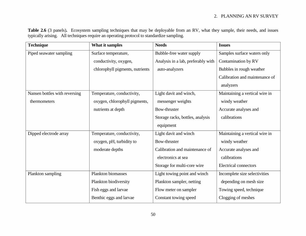
2. PLANNING AN RV SURVEY

50

Table 2.6 (3 panels). Ecosystem sampling techniques that may be deployable from an RV, what they sample, their needs, and issues

typically arising. All techniques require an operating protocol to standardize sampling.

Technique What it samples Needs Issues

Piped seawater sampling Surface temperature,

conductivity, oxygen,

chlorophyll pigments, nutrients

Bubble-free water supply

Analysis in a lab, preferably with

auto-analyzers

Samples surface waters only

Contamination by RV

Bubbles in rough weather

Calibration and maintenance of

analyzers

Nansen bottles with reversing

thermometers

Temperature, conductivity,

oxygen, chlorophyll pigments,

nutrients at depth

Light davit and winch,

messenger weights

Bow-thruster

Storage racks, bottles, analysis

equipment

Maintaining a vertical wire in

windy weather

Accurate analyses and

calibrations

Dipped electrode array Temperature, conductivity,

oxygen, pH, turbidity to

moderate depths

Light davit and winch

Bow-thruster

Calibration and maintenance of

electronics at sea

Storage for multi-core wire

Maintaining a vertical wire in

windy weather

Accurate analyses and

calibrations

Electrical connectors

Plankton sampling Plankton biomasses

Plankton biodiversity

Fish eggs and larvae

Benthic eggs and larvae

Light towing point and winch

Plankton sampler, netting

Flow meter on sampler

Constant towing speed

Incomplete size selectivities

depending on mesh size

Towing speed, technique

Clogging of meshes

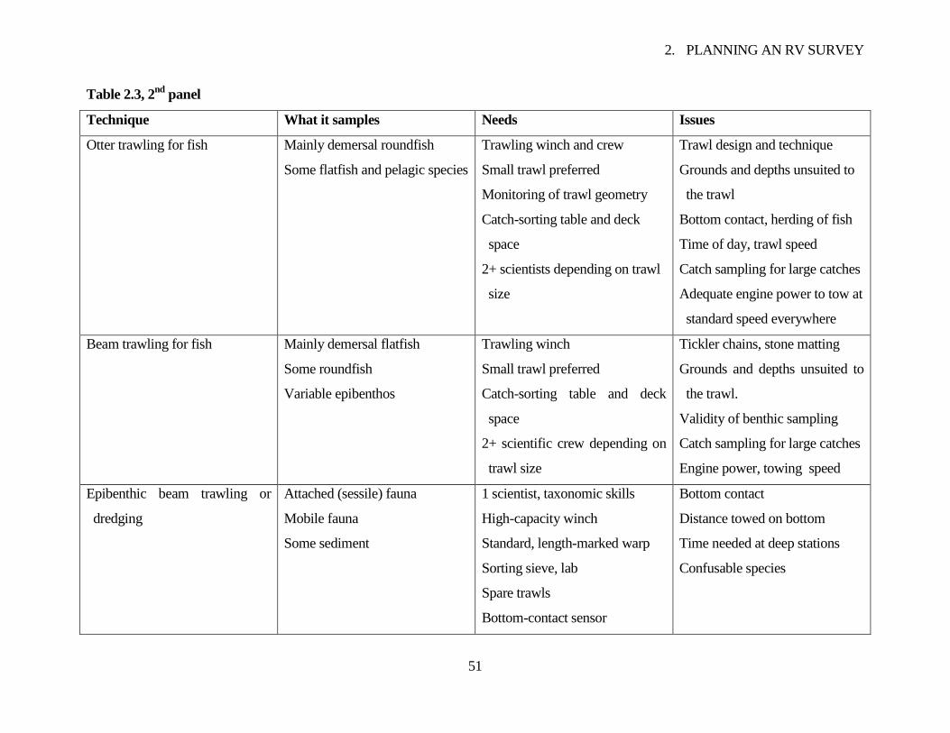
2. PLANNING AN RV SURVEY

51

Table 2.3, 2nd

panel

Technique What it samples Needs Issues

Otter trawling for fish Mainly demersal roundfish

Some flatfish and pelagic species

Trawling winch and crew

Small trawl preferred

Monitoring of trawl geometry

Catch-sorting table and deck

space

2+ scientists depending on trawl

size

Trawl design and technique

Grounds and depths unsuited to

the trawl

Bottom contact, herding of fish

Time of day, trawl speed

Catch sampling for large catches

Adequate engine power to tow at

standard speed everywhere

Beam trawling for fish Mainly demersal flatfish

Some roundfish

Variable epibenthos

Trawling winch

Small trawl preferred

Catch-sorting table and deck

space

2+ scientific crew depending on

trawl size

Tickler chains, stone matting

Grounds and depths unsuited to

the trawl.

Validity of benthic sampling

Catch sampling for large catches

Engine power, towing speed

Epibenthic beam trawling or

dredging

Attached (sessile) fauna

Mobile fauna

Some sediment

1 scientist, taxonomic skills

High-capacity winch

Standard, length-marked warp

Sorting sieve, lab

Spare trawls

Bottom-contact sensor

Bottom contact

Distance towed on bottom

Time needed at deep stations

Confusable species

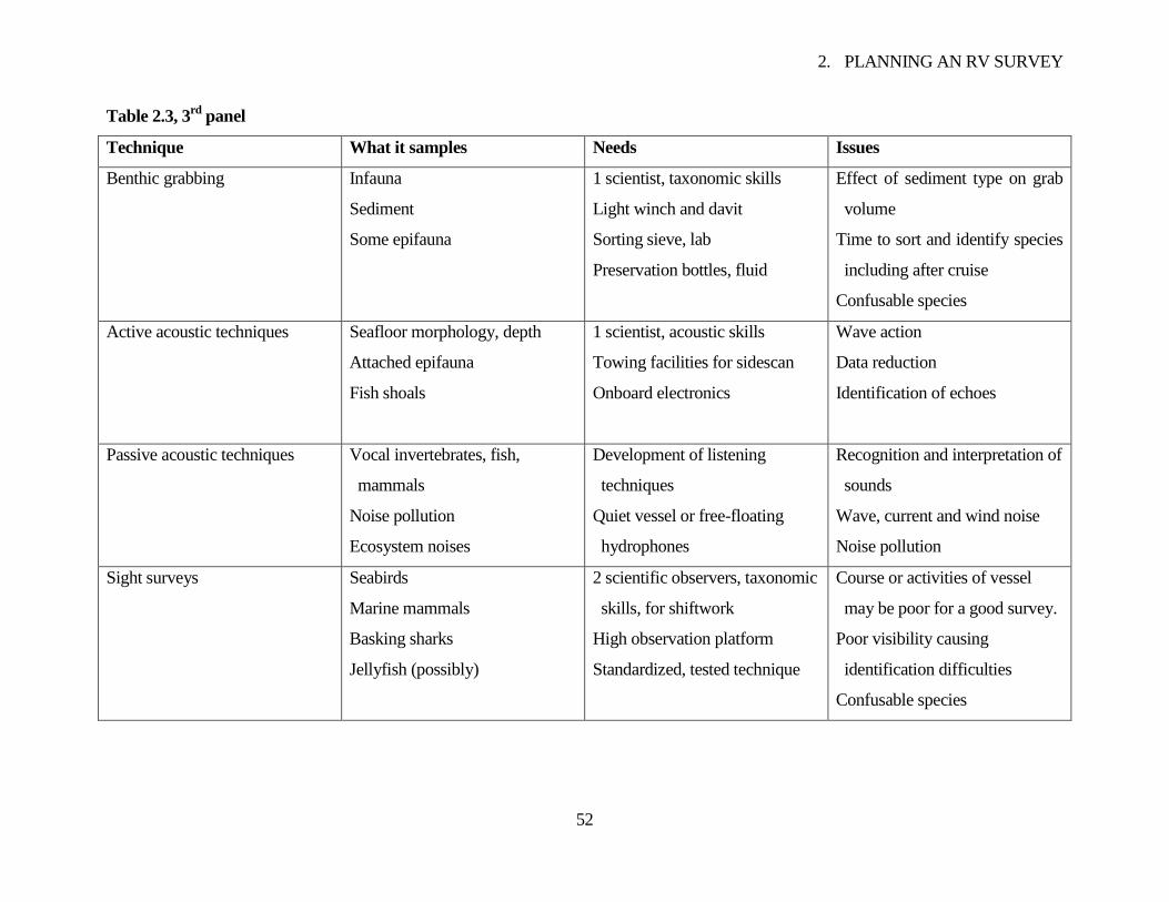
2. PLANNING AN RV SURVEY

52

Table 2.3, 3rd

panel

Technique What it samples Needs Issues

Benthic grabbing Infauna

Sediment

Some epifauna

1 scientist, taxonomic skills

Light winch and davit

Sorting sieve, lab

Preservation bottles, fluid

Effect of sediment type on grab

volume

Time to sort and identify species

including after cruise

Confusable species

Active acoustic techniques Seafloor morphology, depth

Attached epifauna

Fish shoals

1 scientist, acoustic skills

Towing facilities for sidescan

Onboard electronics

Wave action

Data reduction

Identification of echoes

Passive acoustic techniques Vocal invertebrates, fish,

mammals

Noise pollution

Ecosystem noises

Development of listening

techniques

Quiet vessel or free-floating

hydrophones

Recognition and interpretation of

sounds

Wave, current and wind noise

Noise pollution

Sight surveys Seabirds

Marine mammals

Basking sharks

Jellyfish (possibly)

2 scientific observers, taxonomic

skills, for shiftwork

High observation platform

Standardized, tested technique

Course or activities of vessel

may be poor for a good survey.

Poor visibility causing

identification difficulties

Confusable species

2. PLANNING AN RV SURVEY

53

2.5.1 Water sampling

Surface waters can be monitored almost continuously for conductivity, temperature, turbidity,

and nutrients using a piped seawater system connected to an auto-analyser. One scientist will be

needed to keep the system operational and calibrated. A piped supply could be temporarily rigged on

a fishing vessel but practical problems of contamination and bubbling could be challenging.

Subsurface water sampling may be carried out with Nansen reversing bottles (or similar) clipped

to a weighted, depth-marked line lowered from a davit. The bottles are fired by messenger weights.

Water samples for analysis are filled from each bottle as it is returned to the surface, quickly to avoid

temperature changes and loss of gas from solution. A storage area for the sample bottles is needed.

A reversing thermometer and an unprotected thermometer on each Nansen bottle accurately measure

temperature and depth when the bottle is fired. Details of these time-honoured devices are given by

Holden and Raitt (1974, section 7). The RV must be held in position while the Nansen string is out

to prevent excessive wire angles caused by drifting. In windy weather, a bow thruster and accurate

navigation system are important on the RV.

Sub-surface water sampling may be carried out more quickly, though perhaps less accurately,

using a frame to which electrode sensors are attached, eg. for dissolved oxygen, pH, conductivity,

turbidity, depth, and chemical determinands. Calibration and maintenance at sea are time-consuming

skilled tasks, and the whole system may have to be put out of action when one component fails.

Electrical connectors can be especially difficult in salty environments. Depending on how data are

transmitted to the ship, facilities may be needed to wind and store all of the long, multi-core wire that

is lowered over the side with the electrode frame. Some electronic systems are fitted with water

bottles to collect samples for analysis. Agreed oceanographic sampling and calibration methods

should be described in a protocol.

2.5.2 Plankton sampling

Plankton samplers are relatively light sampling devices requiring a davit, winch and warp.

They may be deployed at constant or undulating depths, or hauled up from depth at one location.

Towing should be at a constant speed so that the proportion of fast-swimming animals escaping in

front of the net is standardized so far as possible. The net should be fitted with a flow meter to

measure the volume of water filtered which might be affected by clogging of the meshes. A flow

meter aids quantitative comparisons of results though, as mentioned previously, high variability is to

be expected for plankton samples at the best of times. Given high variability, intensive sampling

2. PLANNING AN RV SURVEY

54

both spatially and in time are likely to be needed to discern trends. A recent text on plankton

sampling and related matters is by Suthers and Rissik (2009). An older reference by Holden and

Raitt (1974) provides still-useful advice. Plankton sampling on an EMS should be covered by a

protocol. The specification should include design of the sampler, netting and meshes, towing speed

and method, estimation of the volume of water filtered, and sample preservation.

2.5.3 Trawling for fish

Demersal trawling on an EMS hosted by a GFS will be governed by the GFS fishing protocols

(eg. Stauffer, 2003, Anonymous, 2009, Anonymous, 2010). Consistency of design, rigging, and

towing technique are just as important for EMSs as they are for GFSs since CPUEs, size and species

selectivities, and even presence-absence proportions will be affected by these factors. Most survey

trawls are either otter or beam trawls, the latter being better when demersal flatfish are the priority.

Midwater trawling is used to verify species compositions during acoustic surveys but is seldom used

by itself for CPUE estimates.

If there is an opportunity to select a trawl design purely for catching demersal and low-

swimming pelagic fish as part of an EMS, the following features would be ideals to aim for:

Simple structure unlikely in future to need redesign and intercalibration.

Short or no sweeps. Effective trawl width is then less affected by variable herding.

Constant geometry despite varying depths and water speeds.

A high headline, especially if the demersal trawl is the only sampler of pelagic species.

Consistent ground contact despite wave motion of the RV, and different ground types.

Rapidly shot and hauled; does not fish at these times.

Achieving all of these ideals is, perhaps, impossible but a Norwegian project reported progress

towards them (Anonymous, 2005, section 2.2).

A survey trawl does not have to be large, nor must it necessarily be towed for long periods

(Pennington and Vølstad, 1991). Large catches mean that catch sampling must be more frequent,

adding a component of sampling variance (Cotter, 1998) and extra work on deck. Smaller trawls

need less engine power to tow and are quicker to deploy, set, and mend when torn. However, the

trawl must be large and heavy enough to sink rapidly and to maintain good bottom contact despite

wave motion of the RV. Also, short, frequent tows waste time on winch work at deep stations and,

for otter trawls, the proportion of towing time when the net is fishing in a stable configuration may be

too low compared to the times taken for the net to stabilize on reaching the seafloor, and to collapse

2. PLANNING AN RV SURVEY

55

on haul-up. Depth-related variations of fishing power can easily arise from variable net geometry; a

common problem is for an otter trawl to spread more widely with a lower headline at depth. Warp-

out to depth ratios are important for configuration and bottom contact, and sensors on the gear,

transmitting acoustically to the RV, permit estimation of configuration and effective towing times.

Towing into the tide is beneficial for achieving constant trawl geometry. A consequence is that the

ground direction of the towing path at a station varies on each visit, thereby randomizing effects of

local ground types on catches at the station. This should help to reduce bias in randomized and grid

survey designs (section 3.2). A recent study of variables affecting otter trawl behaviour for surveys

is by Weinberg et al. (2008).

Trawling speed is another important consideration if not already fixed by a GFS protocol.

Ground speed is most relevant for flatfish and other demersal species that lie close to the bottom.

Water speed is more relevant for actively swimming species. When a multi-vessel RV fleet is used

for an ecosystem survey, all must have sufficient engine power to achieve the selected standard

towing speed into the strongest likely tide. An EMS protocol for a trawl could be derived from, or

styled after a GFS protocol. It should include, trawl design and rigging, towing variables, use of net

monitoring sensors, determination of towing time and distance over the ground, criteria for rejecting

tows, methods of repair, and catch sampling (section 4).

2.5.4 Epibenthic trawling and dredging

Seafloor epibenthos can be sampled with various trawls and sledges that yield a worthwhile

impression of attached and mobile epifauna not obtainable with fishing trawls, benthic grabs or

corers. A lightweight beamtrawl design, has been used informatively in UK waters (Jennings et al.,

1999, Callaway et al., 2007). A slightly heavier, steel-sled design (Ward et al., 2003), and a much

heavier sled intended for rough terrain (Lewis, 2009) have both been applied successfully in

Australian waters (Ward et al., 2006, Currie et al., 2008). Another sled used in Antarctic waters is

given by Brenke (2005). Lightweight designs can suffer from „flying‟ over the bottom resulting in

uncertainties about the effective distance towed. Relevant factors are the weight of the trawl and

warp, ground and water speeds, roughness of the seafloor, depth, and warp-out to depth ratio. Light

trawls also require significant winching times at deep stations. Heavier sampling devices may,

therefore, be best but they are more expensive to build, require bigger winches and a bigger RV to

operate.

2. PLANNING AN RV SURVEY

56

Epibenthic sampling additionally requires a seawater hose for sieving and washing, a well-lit

sheltered working area for sorting catches by low-power microscopy, plus facilities for preserving

and storing specimens, eg. for confirmation of identity. The protocol for epibenthic sampling should

cover design of the trawl or sledge, fishing technique, criteria for rejecting tows, the influence of tide

and weather, processing of the catch including sieve mesh sizes, standardized naming for species that

are not easily distinguished, and training and verification of taxonomic skills of those sorting the

catches.

2.5.5 Benthic grabbing and coring

Benthic grabbing using, for example, a Day grab, yields a large suite of species for monitoring

an ecosystem. It requires a suitable davit with safe, railed space around it to push out and retrieve the

heavy grab over the side. For some sediments, coring may be preferable (Brandt, 2006). Sample

processing facilities required on an RV are the same as are needed for epibenthic sampling, above,

except that sieve meshes are usually finer. Sieving and sorting of benthic samples is time-

consuming. Identifications may not be completed at sea, leaving preserved samples to be sorted

through and identified later. Aside from the extra costs involved, this may delay production of the

ecosystem report, leading to lower interest in it. Protocols should specify the design of the grab or

corer, criteria for rejecting samples, and the other aspects listed for epibenthic sampling, above.

2.5.6 Active acoustic techniques

Biomasses of shoaling pelagic fish species are best estimated by active acoustic methods

combined with midwater trawling to verify species compositions for the returning echoes

(MacLennan and Simmonds, 2010). Sidescan sonar, multi- and single-beam echosounders (Kenny

et al., 2003) are useful for monitoring seafloor habitats. A sidescan fish is towed behind the RV

whereas echosounding techniques are installed in the hull of the vessel. Installed echosounders have

potential to monitor while the RV is steaming. Large volumes of data are then produced which may

have to be sampled for manageability. All these details should be standardized for an EMS

monitoring programme in a working protocol. Oceanographic acoustics is discussed by Medwin and

Clay (1998).

2.5.7 Passive acoustic techniques

Passive acoustic techniques, i.e. listening using hydrophones, have been advocated as

potentially valuable for ecosystem monitoring (Cotter, 2008) though they await development for

2. PLANNING AN RV SURVEY

57

routine use. Many marine species, including fish and invertebrates, make sounds that can be heard

from long distances underwater and that can sometimes be identified, eg.

http://www.fishecology.org/soniferous/justsounds.htm. Libraries of underwater sounds exist (Ranft,

1997) to help. Censusing and distributional studies may sometimes be possible especially when

aggregations of known species are occurring, but many technical problems can arise, eg. selecting the

best frequency bandwidth, interfering noises made by wind, self-noise from water movement over

the hydrophone, shipboard noises, wave-caused bubbles under the ship, and noise pollution from

shipping etc. Free-floating hydrophones, if they can be recovered, might be deployable from RVs.

2.5.8 Sight surveys

Scientists systematically watching6 from an RV can record seabirds, marine mammals and any

other large surface-dwelling animals such as basking sharks. Seabirds are surveyed using either a

fixed-width observation region, or a line transect method that models detection at different distances

from the ship (Buckland et al., 2004, Thomas et al., 2004, Hyrenbach et al., 2007). Possibly other

visible species, such as large jellyfish, could usefully be estimated by similar methods. Watchers can

do their job best if situated well above the sea surface in a sheltered, panoramic observation platform,

eg. the exterior wings of the bridge, or the deck above. Verified taxonomic competence is essential.

A team of at least two watchers working in shifts is best for maintaining alertness, particularly if days

are long. With only one watcher, available watching periods could be sampled. An element of

randomness is then desirable for reducing possible time-of-day biases. Watching protocols should

specify the training and assessment of watchers, describe the watching routine, and clarify what to

record for species that are likely to be confused when seen at a distance, perhaps in poor visibility.

2.5.9 Conclusions

The first choice of sampling technique for an EMS is likely to be demersal trawling which is

suited to most RVs and chartered fishing vessels. A small trawl fished briefly at many dispersed

stations is better for learning about the ecosystem as a whole than a large trawl towed for long

periods at a few stations. There are, however, practical lower limits to trawl size and tow length. In

addition to trawling, oceanographic and plankton sampling may be feasible and appropriate

depending on what is already known about the ecosystem and what is needed to implement an EAF.

6 This could alternatively be called „observing‟ but, in fisheries circles, „observers‟ is a common term for scientists that

accompany commercial fishing trips.

2. PLANNING AN RV SURVEY

58

Acoustic techniques such as single- and multi-beam echosounders and sidescan sonar are

effective for monitoring benthic habitats. Epibenthic or benthic sampling is also needed at intervals

for groundtruth. The latter are informative techniques in themselves for biodiversity, ecological, and

community studies and indicators. Various small trawls, dredges, grabs, and corers are available for

this work. They require appropriate winches, sample sorting facilities, and expertise in benthic

taxonomy. Epibenthic samples are generally quicker to process than infaunal samples.

Sight surveys for seabirds and mammals is feasible from RVs having a suitably panoramic

observation platform, raised above sealevel. Increasing jellyplankton populations is of concern in

some regions and might be monitored by watching or catching methods, though the latter are made

laborious because of the difficulties of cleaning the trawl after each tow. Passive acoustic listening

has been advocated as an additional way of monitoring vocal marine animals. However, techniques

require development for monitoring purposes.

All sampling methods required detailed protocols so that different scientific crews can

standardize their work on every RV monitoring cruise. Taxonomic skills and thorough training in all

sampling techniques are critical for EMSs. The occurrence of confusable species should be expected

and dealt with by naming them in standard ways.

3. ECOSYSTEM SURVEY DESIGN

59

3 ECOSYSTEM SURVEY DESIGN

Ecosystem monitoring surveys (EMSs) carried out in collaboration with groundfish or acoustic

surveys must make the most of the fishing stations and course chosen to meet their priority objectives

of estimating stocks of commercial species. Ecosystem sampling is then opportunistic and survey

design is hardly an issue. Designing an independent EMS, on the other hand, raises several issues

addressed in this section.

A preliminary note on some terminology preferred in this report is needed. Generally, „region‟

refers to geographic areas, so the „surveyed region‟ is the geographic area just enclosing all of the

sampling stations chosen for a survey, possibly with holes where localities are inaccessible for

sampling. Sometimes, however, the time dimension should be remembered as well because RVs

tend to travel slowly relative to marine distances such that results at one edge of the surveyed region

may differ from those at the opposite edge not only because of their geographic separation but also

because of the seasonal difference between the dates of sampling. Similarly, species and fisheries

may also vary their regions of presence or activity over time. For these reasons, the word „domain‟ is

used to refer to a region plus an associated period of time even though, for operational reasons, the

time dimension may have to be ignored.

The first task of designing an EMS is to locate the survey domain with respect to the defined

ecosystem (section 2.1). The next is to choose a survey design. Three statistical designs are put

forward. One, based on randomly located stations, is intended for reliable estimation of indicators as

summarizing statistics, eg. the mean or median, for the whole survey domain, or for specified sub-

domains. The second, based on an even grid of stations, is intended when spatial modelling, eg.

contouring, is the primary objective. Since both designs have weaknesses when applied for the other

purpose, a third, compromise design, using a lattice of square sampling strata, is proposed. None of

these designs is „optimal‟ in the sense of producing as much information per unit cost as possible.

Optimization is likely to be fruitless for an EMS because a design good for one species will almost

certainly be disastrously inefficient for many others. Instead, general utility for most priority species,

low bias, adaptability for regional estimation or modelling, and practicality are all treated as more

relevant than statistical efficiency for designing an EMS.

3. ECOSYSTEM SURVEY DESIGN

60

3.1 Choosing the survey domain

The survey domain of an EMS may not match the boundaries of the ecosystem if (i) the

ecosystem is too big to contemplate sampling throughout, eg. it is an ocean; (ii) if parts of it are

inaccessible, eg. they are too rocky, deep or steep; or (iii) there are reasons for positioning some

sampling stations outside the named ecosystem anyway, eg. to deal with migrating species.

Knowing the relationship between the survey domain and the domains occupied by the

individual species being surveyed can be important for interpreting survey results, as well as for

understanding why average catch rates for some are much more variable than for others. The region

occupied by a species at any point in time varies due to migrations, expansion or contraction of the

population, or because different stages of the life cycle occupy different places. Figure 3.1 illustrates

some possible relationships between survey domains and a species‟ domain when migrations occur.

Total enclosure of a species by a survey is easiest to interpret, though results may still depend on the

whereabouts of the species with respect to the pattern of sampling stations. Partial overlap is less

straightforward because the sub-population monitored inside the survey domain may differ from that

outside, causing bias in results for that species. Migrations across the survey boundary, eg. with

season, year, and/or age (Trenkel and Cotter, 2009), can add variance to the survey results as well,

particularly if the migrations themselves vary in relation to the seasonal time period of the EMS.

Estimates of abundance- and size-related indicators could be strongly affected. Precision is worst

when the overlap between survey and species domains is small, with only a small number of

sampling stations present within the overlap.

Bounding the survey domain so as to minimize bias and variance arising from partially

overlapping domains of priority species could be assisted by developing a „Species database‟ holding

details of the regions occupied seasonally, preferred habitat types, and migrations of each species.

For simplicity, irregularly shaped regions could be simplified to rectangular enclosures, bounded by

N and S latitudes and E and W longitudes marking the limits of the actual boundaries, perhaps with

one set of four points for each quarterly season to allow for seasonal migrations. Candidate survey

domains can then be quickly tested to see which species are likely to be enclosed, which overlapped

partially, and which would be overlapped variably depending on migrations. Such a database would

also form a valuable resource in its own right and could be updated as the survey time series

lengthens, possibly leading to marginal revisions of the survey domain. Table 3.1 suggests fields for

a Species database, including others mentioned later in this report.

3. ECOSYSTEM SURVEY DESIGN

61

Choosing the best season or seasons for an EMS also needs care. For priority species and

certain biological indicators, the seasons of migrations, reproduction, recruitment, and growth may

affect whether the survey is informative or, at worst, misleading. Compromises and trade-offs

between species are likely. Allocating available RV-days across different seasons, rather than to one

seasonal cruise in each year is another option to consider. Fewer stations would be fishable on each

cruise but more types of indicator may be measurable over the year giving, perhaps, a more

informative survey overall. Concerning terminology again, in this instance, one repetition of a

„survey‟ consists of more than one „cruise‟.

The definition of the survey domain in the EMS protocol may exclude different types of ground

or depths, or may include them subject to sampling with different types of catching device so as to

catch priority species with best efficiencies. For example, an otter trawl might be rigged differently

for hard and soft, or shallow and deep grounds. Intercalibration of the different gears and

configurations would not usually be feasible for all species. However, since catchabilities and size

selectivities differ from species to species even for a single type of gear operated in one way, using

different sampling gears for different types of ground, provided it is done consistently for every

repetition of the survey, would not add much to the problems of interpreting EMS results but would

allow more of the ecosystem to be sampled consistently. So, for example, swapping a dredge for a

grab at certain stations may be a practical way of retrieving constant volumes of sediment. The EMS

protocol should state if certain regions or stations are to be sampled with particular types of gear so

that it is done in the same way on every repetition of the survey.

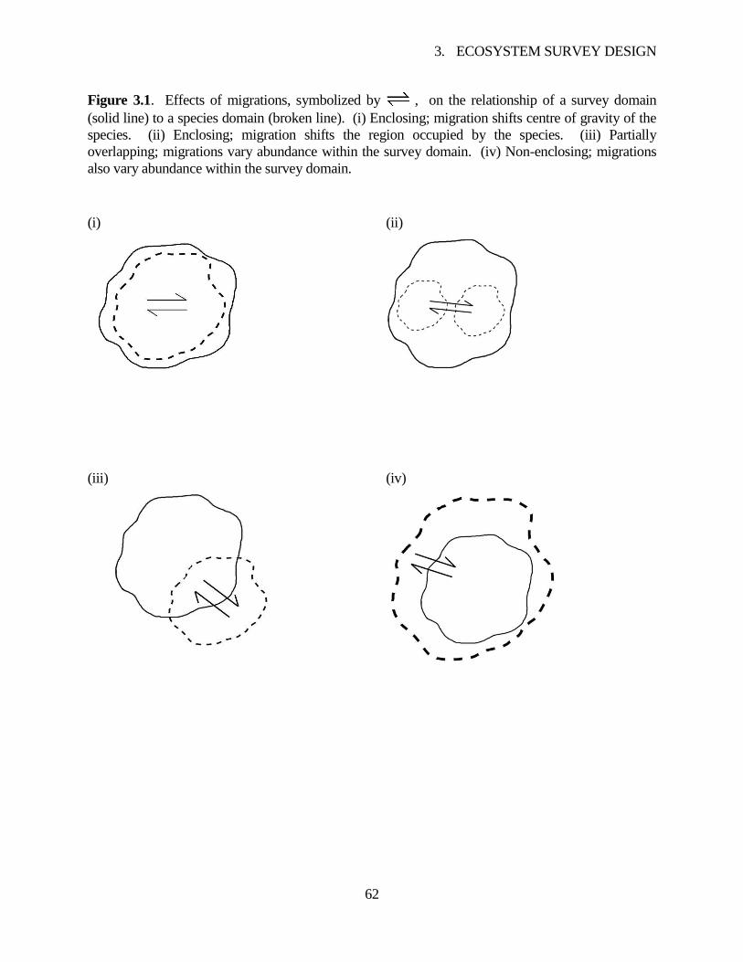
3. ECOSYSTEM SURVEY DESIGN

62

Figure 3.1. Effects of migrations, symbolized by , on the relationship of a survey domain

(solid line) to a species domain (broken line). (i) Enclosing; migration shifts centre of gravity of the

species. (ii) Enclosing; migration shifts the region occupied by the species. (iii) Partially

overlapping; migrations vary abundance within the survey domain. (iv) Non-enclosing; migrations

also vary abundance within the survey domain.

(i)

(ii)

(iii)

(iv)

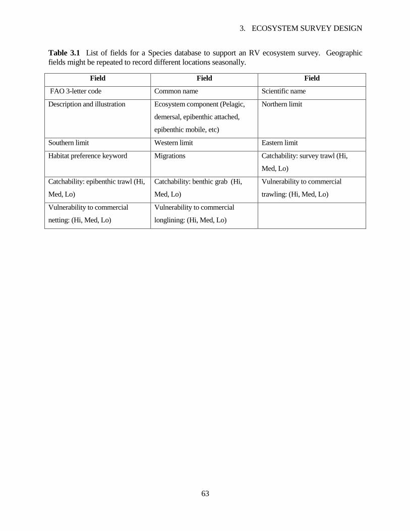
3. ECOSYSTEM SURVEY DESIGN

63

Table 3.1 List of fields for a Species database to support an RV ecosystem survey. Geographic

fields might be repeated to record different locations seasonally.

Field Field Field

FAO 3-letter code Common name Scientific name

Description and illustration Ecosystem component (Pelagic,

demersal, epibenthic attached,

epibenthic mobile, etc)

Northern limit

Southern limit Western limit Eastern limit

Habitat preference keyword Migrations Catchability: survey trawl (Hi,

Med, Lo)

Catchability: epibenthic trawl (Hi,

Med, Lo)

Catchability: benthic grab (Hi,

Med, Lo)

Vulnerability to commercial

trawling: (Hi, Med, Lo)

Vulnerability to commercial

netting: (Hi, Med, Lo)

Vulnerability to commercial

longlining: (Hi, Med, Lo)

3. ECOSYSTEM SURVEY DESIGN

64

3.2 Statistical terms and inference

Having decided the survey domain, sampling stations must be allocated within it. The term

„sampling unit‟, taken from Sampling Theory, is used here to mean the smallest practical unit of

sampling for any gear, eg. the multi-species catch of a trawl, the mixed contents of a grab or water

bottle, etc.. The term, „sample set‟ is used to refer to a collection of N sampling units. [The word

„sample‟ is avoided when there can be ambiguity between a sampling unit or a sample set.]

„Sampling‟ is used to refer to the process of collecting a set of sampling units by an EMS.

Fish and benthic survey design is often controversial (e.g. Anonymous, 2004). Nevertheless,

Sampling Theory implies that we may infer the properties of a marine region from the properties of a

set of N sampling units with either of two contrasting approaches (eg. see Thompson, 1992):

Design-based inference: It assumes a randomized statistical design but nothing about the

nature of variation in the population. It serves best when regional estimation of

summarizing statistics, eg. means or medians, are the priority.

Model-based inference: It assumes a mathematical model of spatial variation and, perhaps,

other factors such as temperature, but assumes nothing about the sampling design. It serves

best when a model of spatial variation, eg. a set of fitted contours, is the priority.

Of course, both approaches are ideals: sampling is never perfectly randomized in practice, and

models never fit real variation perfectly. The contrast between them raises the possibility of a third,

compromise approach referred to here as lattice-stratified sampling. All three are discussed in the

sub-sections below but, firstly, another approach, referred to as „Station-based sampling‟ is

described because of its popularity. Arguments for dismissing it from further consideration are

given. More statistical matters are covered in a later section on data analysis (section 6).

3.3 Station-based sampling

„Station-based‟ sampling refers to the practice of taking replicate sampling units at each visited

station so that, by using analysis of variance, a „within-station‟ standard error can be estimated and

applied to abundances, biomasses, or other measures made at any single station. The main

assumption underlying station-based sampling is that a fixed statistical distribution and variance

parameter are common to every station and, therefore, are worth estimating. Reasons to doubt this

assumption are:

3. ECOSYSTEM SURVEY DESIGN

65

High spatial heterogeneity and patchiness are typical in marine environments at all scales.

The population of possible sampling points at a station is poorly defined because it varies

with the accuracy of navigation, wire angles, wind and currents, and the direction of towing

in the case of a trawl.

The number of sampling units taken at each station is typically small, e.g. 3 to 5, meaning

that neither the constant variance assumption nor the validity of any transformation applied to

achieve it can be verified.

If the assumption of a fixed statistical distribution at every station is in serious doubt, there is no

point in estimating a station-based variance because it itself is expected to vary throughout the

sampling domain. Additionally, a major practical drawback of replicate sampling is that fewer

stations can be sampled with the available RV resources. Consequently, the survey captures less of

the spatial and temporal variability existing within the survey domain. For these reasons, station-

based sampling is not recommended.

3.4 Design-based regional estimation

„Regional estimation‟ refers to estimation of parameters defined for a specific domain, R, from

sampling units located within it. R could either be the survey domain itself, or a single stratum

(subdivision of the survey domain), with an associated time period spanning the time period of the

survey. In practice, the time dimension may be ignored for operational reasons. The word „regional‟

estimation is used here because it is used in Geostatistics. The parameters could be means, medians,

variances, or others.

Design-based regional estimation requires that sampling stations be located at randomly chosen

space-time co-ordinates. Station co-ordinates, northings and eastings, are picked with a table of

random numbers (the uniform distribution of Statistics), rejecting those that fall outside the survey

domain, eg. beyond the boundaries, or on unfishable ground previously excluded from the survey

domain (section 3.1). Station co-ordinates should be freshly randomized for each repetition of the

survey so that the residual errors will average to zero over time. If this is not done, the residual error

associated with each repetition of a survey must be assumed constant and not a function of the value

of any measure found, a weakness of the design. Repeated use of a single random selection of

stations is most accurately referred to as a fixed-station design.

3. ECOSYSTEM SURVEY DESIGN

66

Randomizing in time is usually not practicable for an RV that, because of limited speed and high

fuel costs, must visit the next adjacent sampling station, more or less in sequence. If so, timing must

be assumed to have no effect on measured results, as may be true for some indicators but not others

such as indicators of reproduction and growth which could be highly seasonal (section 5.1.4).

Depending on the configuration of stations and distances between them, there may be opportunites

for randomizing the cruise track without undue additional expense and time. If so, they should be

used. A different cruise track for each repetition of a survey is desirable for avoiding enduring

confounding over a time series between timing and locality of sampling.

The true regional parameters of R are defined as sums for countable populations such as fish,

and as integrals over area and time for continuous variables such as concentrations in water, or

sedimentary properties. See Box 3.1.

Randomization of sampling within R confers the benefit that estimates of R‟s parameters are

expected, from Sampling Theory, to be unbiased, meaning that histograms of repeated estimates, ie.

made from different sets of N randomly located stations, are centred on the defined parameter. In

addition, increasing N causes the statistical distribution of the sample mean, y , to tend toward the

Gaussian (normal) shape with variance reducing in proportion to N in accordance with the Central

Limit Theorem (Feller, 1968), provided that results at each station are kept independent (section

6.2.5). The value of N needed to achieve reasonable approximation to Gaussian depends on the

probability of occurrence of extreme positive values of y; there can be no standard guidelines.

The most basic design for a regional survey is simple random sampling (SRS). It permits

straightforward estimation of means, variances, medians or other quantiles etc. using formulae from

textbooks. A disadvantage is that it usually gives an uneven spread of stations within a region,

possibly prompting criticism that the sample set is “unrepresentative”, or that it favours some species

more than others depending on their domains. It can also cause practical difficulties with catch-

processing work because of unequal steaming times between adjacent stations. Stratified random

sampling (StrRS) can be designed to provide a more even spread of stations. The survey domain is

divided into sub-domains, called strata, having similar areas. Each is sampled at the same rate, ie. it

receives the same number of sampling stations per unit of area. This is „proportional allocation‟.

If, alternatively, evenness is not so important, strata may be designed to enclose and isolate

major features of the ecosystem such as habitat types, depth ranges, or zones of upwelling. The strata

may then have very different areas. Selected strata receive higher sampling rates to reflect their

3. ECOSYSTEM SURVEY DESIGN

67

importance and expected variance. This strategy may be maximally informative about the effects of

the features but may diminish precision for other important estimates not linked to the features, and

could still suffer from irregular steaming times between stations.

The number of strata used in a survey is a compromise for a given total of N stations. More

strata offer increased spatial definition but the number of stations in each is reduced, leading to

reduced precision of estimation. A small number of strata, on the other hand, improves precision but

decreases spatial definition. However, the latter strategy improves the Gaussian approximation

offered by the Central Limit Theorem because fewer strata mean fewer parameters to estimate and

higher degrees of freedom for estimating variances. Restraining the numbers of strata therefore

seems the more dependable and informative strategy for regional estimation even if, at first sight, a

survey appears to offer less spatial detail as a result. Large numbers of strata can be thought of as a

luxury only justifiable if there are resources for large numbers of stations to be sampled in each.

The weighting of regional strata for calculation of StrRS estimates of mean values for the whole

survey domain (Cochran, 1977) depends on how estimates are calculated in each stratum (Cotter,

2009b). For countable populations such as fish and benthic invertebrates, the measure on each fish,

say, can be averaged over all fish in a stratum. This is called the „mean over fish‟. Alternatively, the

measure can be averaged for all the fish at each station, and the stratum mean estimated as the mean

of the station means. This is called the „mean over stations‟. The two estimators are explained in

more detail in Box 3.1. For over-fish estimation, the strata are, for logical consistency, weighted by

the numbers caught in each. The stratum weights would then vary from species to species, as may

seem reasonable. For over-stations estimation, the strata are weighted by area. The areas should be

accurately measured. Weighting of strata for uncountable populations is simpler than for countable

populations because there is no clustering of unmixed individuals in a sampling unit. See Box 3.1.

Area-based stratum weights are therefore appropriate for uncountable measures such as temperatures,

concentrations, etc.. Having decided the best stratum weights, means, variances and other

summarizing statistics can be estimated straightforwardly and without bias using textbook StrRS

formulae (Cochran, 1977, Thompson, 1992). The distributions of means for the total survey domain,

like those for the strata, approach normality for large N by the Central Limit Theorem.

3. ECOSYSTEM SURVEY DESIGN

68

Box 3.1. Defining and estimating parameters for populations monitored

by an EMS

Countable populations

‘Countable populations’ in aquatic environments refers to animals such as fish. Two approaches and a

compromise have been suggested (Cotter, 2009b) for defining the parameters of countable populations, the

gist of which is below.

One approach is to define regional parameters as if individuals of the population are the sampling units.

So, for the mean of variable, y,

1

1

Npop jjY N y (1)

for which the statistically consistent estimator is found ‘over fish’ (or whatever animal it is):

1 1

stn in niji j

fishfish

yy

n (2)

stnn is the number of stations indexed by i , in is the number of fish caught at each, and fishn is the total

number caught. Estimator (2) is an average weighted by the number of fish caught at each station. It implies

that zero catches are irrelevant, that the best estimate is obtained by sampling at stations where the species

is common and, when the survey is stratified, that the strata should be weighted by numbers of fish caught,

assuming that they are the best available estimates of relative population sizes.

The other approach is to define a regional parameter in a geographic sense with the survey domain

divided into a grid of A small plots treated as sampling units. Then, if there are an fish in the a ’th plot, and

1an

a ajjy y ,

1

1

Aaa

geog Aaa

yY

n (3)

Definitions (1) and (3) are identical in value but, since individual animals cannot usually be sampled

independently, (3)fits better conceptually with the catching of clusters of animals in a net or other device

deployed at a station by an RV. The statistically consistent estimator is ‘over stations’:

1stnn

iistn

stn

yy

n (4)

3. ECOSYSTEM SURVEY DESIGN

69

In contrast to estimator(2), estimator (4) weights the mean value at each station equally regardless of the

number of fish caught. It implies that stnn should exclude stations where catches are zero; the estimate is

then for the mean of y over that part of the species domain within the survey domain. Estimator (4) also

implies that many stations should be spread around to capture geographic variation and, when the survey is

stratified, that the strata should be weighted by areas.

As a compromise, a mixed-model estimator has been suggested:

ˆ ˆ1mix stn fishy y y (5)

where ˆ is the within-catch correlation estimated by fitting a mixed model to results by station. If quantiles,

eg. the median, are preferred as summarizing statistics because they minimize the influence of outlying

(extreme) results, the same weighting considerations apply. For details, see Cotter (2009b).

Uncountable populations

Continuous variables such as concentrations can be thought of as ‘uncountable’ populations for

sampling purposes. Regional parameters can be defined as integrals over the region, R . Let the area of R

be RA . Then, for example:

Mean: 1 .R R R

A y dA

Variance: 22 1 .R R RR

A y dA

Median: R for which . .R RR Ry dA y dA

Sampling units usually only provide one measurable value, iy at station i , for a continuous variable because

the content of the sampling unit, eg. a bottle, is mixed before measurement. Therefore within-sampling-unit

correlation is not a problem and estimators can be taken from standard sampling texts (eg. Thompson,

1992). For example, the estimator for R is, as usual,

1stnn

iiR

stn

yy

n (6)

Estimates of the mean using (6) improve in precision as the number of stations located independently

and randomly within R increase. They also tend to the normal distribution under the Central Limit Theorem,

allowing confidence limits to be estimated from standard errors. Sample medians can be dealt with using

binomial confidence limits (Conover, 1971, Cotter, 1985) which also get narrower as N increases.

3. ECOSYSTEM SURVEY DESIGN

70

3.5 Model-based estimation with a grid of stations

For model-based estimation, the survey domain is imagined as an uncountable population of

points, on each of which one or more variables, eg. density, can be measured. Values of the variables

are governed by a mathematical function, called a model, of spatial co-ordinates and, maybe, other

factors, eg. temperature or season. Estimation of the model‟s parameters depends on it adequately

simulating all spatial and factor-related variation. Then the values observed on a set of N sampling

units should form residual errors falling around the fitted model with a random, non-spatial pattern.

No assumptions about the sampling design are made because, by definition, all variation is in the

model and none can be caused by „biased‟ sampling. Contours and other general spatial models

suitable for gridded stations are available in global information system (GIS) software packages. See

also the open-source R system (Bivand et al., 2008) and a review of digital mapping methods in

fisheries science by Eastwood et al. (2008).

The most obvious choice of survey design for model-based inference is a regular grid of stations

spread as densely as RV resources allow across the survey domain. Then the model is estimated with

the same density of information in every locality. The starting point and orientation of the grid – it

does not have to align with the compass points – can be randomized for each repetition of the survey

in order to average out, or expose factors unwittingly omitted from the model. However, there are

only 2 degrees of freedom, possibly causing a large between-repetition variance.

Many scientists are happy to estimate means, medians, variances and other descriptive statistics

from grid surveys but they risk bias from the restriction on randomization imposed by the grid, in

particular from trends over the domain, and from cyclical variability having periods „aliased‟ with the

distance between lines of stations in the grid (Cochran, 1977). See Figure 3.2 for an explanation.

Also, degrees of freedom are less than a count of the number of stations in the grid because of serial

dependence of results at neighbouring stations. Using the number of stations to estimate a regional

variance, for example, would give an estimate that is biased too low. A particular problem from

using a regular grid for an EMS arises for a species with a falling population that contracts its species

domain into favoured, localized habitats falling between stations in the grid and, thus, not reached by

the EMS.

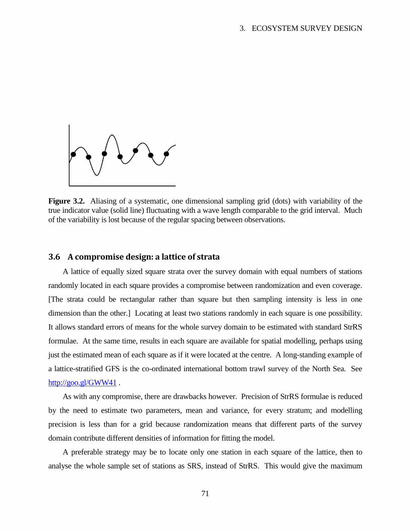
3. ECOSYSTEM SURVEY DESIGN

71

Figure 3.2. Aliasing of a systematic, one dimensional sampling grid (dots) with variability of the

true indicator value (solid line) fluctuating with a wave length comparable to the grid interval. Much

of the variability is lost because of the regular spacing between observations.

3.6 A compromise design: a lattice of strata

A lattice of equally sized square strata over the survey domain with equal numbers of stations

randomly located in each square provides a compromise between randomization and even coverage.

[The strata could be rectangular rather than square but then sampling intensity is less in one

dimension than the other.] Locating at least two stations randomly in each square is one possibility.

It allows standard errors of means for the whole survey domain to be estimated with standard StrRS

formulae. At the same time, results in each square are available for spatial modelling, perhaps using

just the estimated mean of each square as if it were located at the centre. A long-standing example of

a lattice-stratified GFS is the co-ordinated international bottom trawl survey of the North Sea. See

http://goo.gl/GWW41 .

As with any compromise, there are drawbacks however. Precision of StrRS formulae is reduced

by the need to estimate two parameters, mean and variance, for every stratum; and modelling

precision is less than for a grid because randomization means that different parts of the survey

domain contribute different densities of information for fitting the model.

A preferable strategy may be to locate only one station in each square of the lattice, then to

analyse the whole sample set of stations as SRS, instead of StrRS. This would give the maximum

3. ECOSYSTEM SURVEY DESIGN

72

geographic spread of stations while each point in the survey domain has an equal probability of

observation. For the purposes of SRS, this is not quite the same as giving every possible sample set

of N stations an equal probability of observation, as SRS estimation formulae require for elimination

of bias (Thompson, 1992). The difference is the restriction on randomization attributable to

analysing the lattice-stratified design as an SRS, instead of as a StrRS. It seems a subtle difference

that is unlikely to cause much bias, and certainly less than a grid design in which randomization has,

at most, 2 degrees of freedom, as discussed above. In summary, a lattice design with one station per

square has the valuable advantages for an EMS of providing even coverage, opportunities for spatial

modelling, and simple, though slightly biased estimation by SRS formulae.

3.7 Conclusions

Ecosystem surveys differ in several respects from groundfish surveys focussed on commercial

fish species. Ecosystem surveys enclose the domains of some species but only overlap those of

others, potentially adding bias and sampling variance to results for the overlapped species,

particularly if there are few stations in the overlapping region. Bounding the survey domain before

designing the survey should take into account the distributions of priority species and could be

assisted by a Species database holding distributions, migrations, and habitat preferences for each

species. Retrievals could then quickly show which species will be enclosed, and which merely

overlapped by candidate survey domains. The database would also serve as a store of species

knowledge. An ecosystem monitoring survey is likely to use several different sampling devices so

the boundaries of the survey domain should also take into account access, and adequacy of sampling

on different types of seafloor by them. The season of an EMS must be carefully chosen because

many indicators are sensitive to seasonal growth, temperature, migrations, and reproductive cycles.

Different catching devices are unlikely to be intercalibrated for different catchabilities for each

species, implying that caution is needed when interpreting or using multispecies data from an EMS.

Replicate sampling at individual stations is not recommended because of the environmental

heterogeneity typically existing, and the need to spread as many stations as possible widely around

the survey domain. Instead, regional estimation with design-based, randomized sampling schemes is

proposed for estimating means, medians, or other parameters defined for specific marine regions or

domains. Standard errors and confidence limits are justified by large samples and the Central Limit

Theorem with minimal dependence on unsafe assumptions, e.g. constant standard errors at different

stations. Sampling may be stratified so that evenness of coverage is better than for simple random

3. ECOSYSTEM SURVEY DESIGN

73

sampling, or so that major features of the ecosystem, eg. different habitats, are isolated if this is

thought to be more informative for EAF. The number of strata should be low with many stations in

each for maximum precision and dependability of EMS results. Care is needed in choosing stratum

weights and station allocations.

Model-based estimation is proposed when EMS results will be analysed by fitting a model, eg.

contours. Provided that there is confidence that the model includes most significant variation,

stations can be set out in a regular grid so that equal densities of information are used for fitting the

model over each part of the survey domain. The grids should be re-positioned at a randomly chosen

starting point with a random orientation for each repetition of the survey. Summarizing statistics, eg.

the mean, can be estimated from gridded survey data but there is a risk of bias because of the strong

restriction of randomization.

A compromise between randomized and grid designs is obtained with a lattice of equally sized,

square strata with one station per square. Design-based estimation uses simple random sampling

formulae as if there were no strata, and spatial modelling benefits from an even spread of stations

across the survey domain. The strengths of a lattice-stratified design appear to outweigh its

weaknesses for a multi-species, multi-objective EMS.

4. PROCESSING CATCHES AT SEA

74

4 PROCESSING CATCHES AT SEA

An RV ecosystem monitoring survey (EMS) may operate two or more catching devices, eg. a

demersal trawl and a grab, and may yield tens or hundreds of species of interest from each. Sorting,

identifying, quantifying, and taking measurements on many priority species therefore requires

significant scientific labour. Since this work, along with other duties at each station, must normally

be completed by the time the next catches are ready to be brought on board, catch processing may

have to be restricted so that the same set of tasks can be completed reliably at every sampled station

despite foreseeable problems such as bad weather, net repairs, and exceptionally large catches. This

cautious approach to setting the amount of work is important because the final product of an EMS,

namely time series of measures and indicators, are generally much more informative if they do not

suffer from missing values and erratic precision, both of which would be caused by inconsistent

catch processing. A consequence is that, when catches are light and everything is going well, the

scientific crew may have a little spare time . . . for non-routine duties.

The first two sub-sections below briefly consider the initial cleaning and sorting of catches into

species, whether taken by trawls or other catching devices. Figure 4.1 schematically illustrates these

initial processing stages applied to the catch of an otter trawl.. The third sub-section considers

sampling of species or size groups for estimation of indicators. The fourth puts forward ideas for

matching indicators to the level of catch processing and for getting the most information from them.

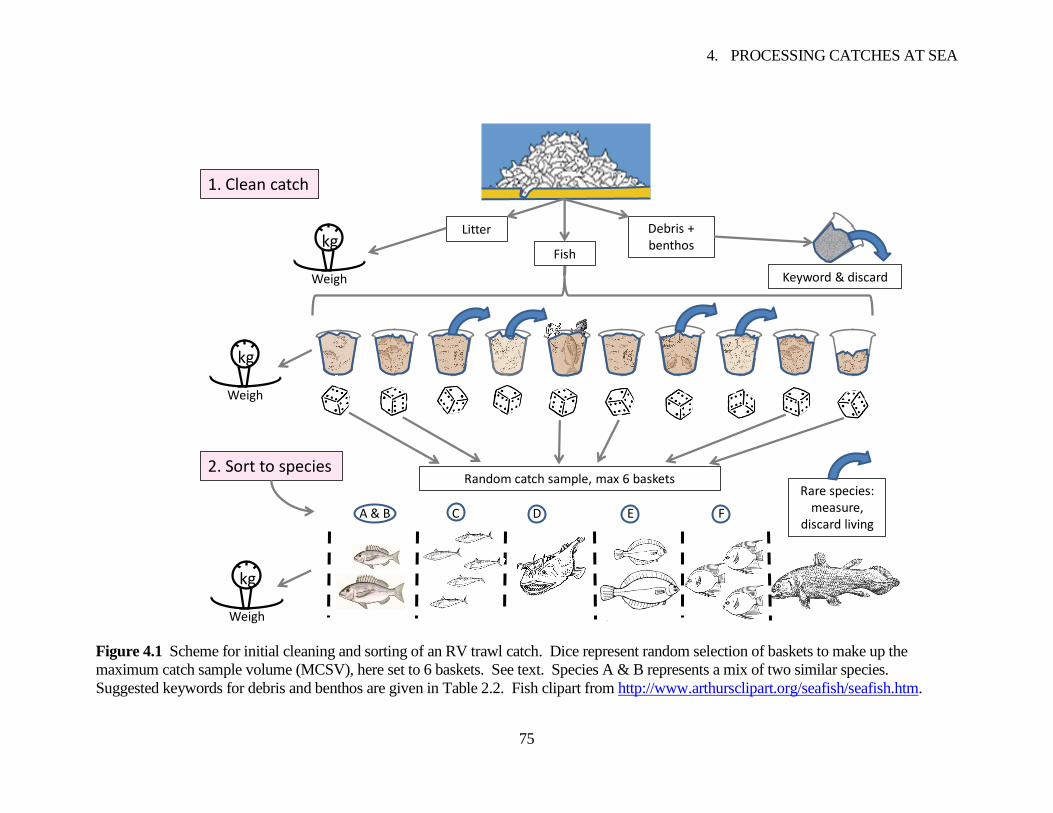
4. PROCESSING CATCHES AT SEA

75

Figure 4.1 Scheme for initial cleaning and sorting of an RV trawl catch. Dice represent random selection of baskets to make up the

maximum catch sample volume (MCSV), here set to 6 baskets. See text. Species A & B represents a mix of two similar species.

Suggested keywords for debris and benthos are given in Table 2.2. Fish clipart from http://www.arthursclipart.org/seafish/seafish.htm.

A & B

Litter

Fish

Debris + benthoskg

Weigh

Random catch sample, max 6 baskets

Keyword & discard

Rare species:measure,

discard livingC D E F

2. Sort to species

1. Clean catch

kg

Weigh

kg

Weigh

4. PROCESSING CATCHES AT SEA

76

4.1 Cleaning the catch

Living biological material in a catch should firstly be separated from sediment, rocks, dead

shells, and any other debris either initially or as part of the processing to separate species. „Debris‟

could sensibly include living material for which the catching device was clearly never intended, eg.

sundry epibenthic species caught in an otter trawl, or occasional large fish taken in a small epibenthic

trawl. Few if any inferences can be drawn from such occasional occurrences. Quantifying sediments

and rocks caught would also be an unproductive use of time, though descriptive keywords could be

helpful for mapping benthic habitats. See Table 2.2, page 35. On the other hand, keeping a record of

quantities and types of litter items is relevant for an ecosystem survey (Galgani et al., 1995, Galil et

al., 1995)7. Material other than litter can be washed overboard but only when the vessel is not

trawling. Biological material should only be discarded when sight surveys for seabirds will not be

disturbed.

4.2 Separating species

The next stage of processing is separation of the biological material by species. A strong sorting

table or channel lined with stainless steel sheet is ideal. Poor standards of identification remarked

upon for European GFSs (Daan, 2001) underline the magnitude of the taxonomic task for an EMS

for which identification of many more species is important. Scientists should be thoroughly trained

and objectively tested in the necessary branches of taxonomy before being permitted to name species

on an EMS. Training and testing should be outlined in the catch-processing protocol.

Species identification is time-consuming when biodiversity is high so complete identification

may not be feasible at every station. The catch-sampling protocol could specify a list of all species to

be processed on the EMS; specimens of unlisted species are merely preserved for later identification

so as to control the need for ad hoc taxonomic research during catch processing. In addition to

saving time, a list should prevent inconsistent processing of unusual species on some cruises but not

on others as a result of the personal interests of those who happen to be on board. Such

inconsistencies could give misleading indications of the recurrences of species.

When sampling a large catch, the chance of finding a rare species increases with the amount of

catch searched, particularly if the species is small or unobtrusive. Setting a „maximum catch-

sampling volume‟ (MCSV) in the catch-processing protocol is suggested as a way of dealing with

7 See also http://www.chrisjordan.com/gallery/midway/#about

4. PROCESSING CATCHES AT SEA

77

occasional very large catches consistently and within time limits. 6 randomly drawn baskets is

shown as the MCSV in Figure 4.1, but the MCSV should generally be as large as catch-sorting

resources allow. Then the total catch, or the MCSV, whichever is the smaller, would be searched

thoroughly at every station for rare species at the same time as it is sorted into species. An MCSV

could help to standardize the apparent catchabilities of rare species, leading to better standardized

occurrences, CPUEs, and diversity measures.

Species that are not easily identified are likely to occur frequently on ecosystem surveys, either

singly or as mixes of two or more species that are hard to separate. Many of the difficult groups and

combinations are foreseeable, given experience, and standard procedures for dealing with them

should be prepared for catch-processing protocols. A mix of two or more similar species can be

collected when sorting a large catch, and the ratio of the species estimated by detailed examination

of a randomly drawn sample set from the shuffled mix. The size of the sample set needed will

depend on whether the ratio of species is all that is required, or whether LFDs are required for each

species individually. See Figure 4.2. Perhaps not all species‟ mixes merit this extra work and, if not,

a standardized, common taxonomic name for any individuals of the group of confusable species

should be written into the protocol. The same applies to single species that are hard to identify to the

species level; the acceptible taxonomic name should be specified in the protocol, eg. „Genus sp‟.

Inconsistent naming, as inevitably occurs among different workers not guided by agreed naming

rules, is likely to result in the species group being lost or confused in a database.

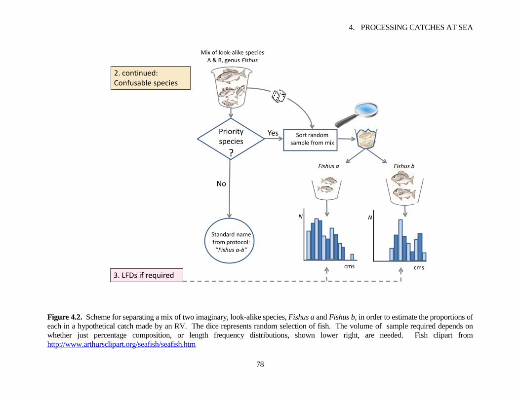
4. PROCESSING CATCHES AT SEA

78

Figure 4.2. Scheme for separating a mix of two imaginary, look-alike species, Fishus a and Fishus b, in order to estimate the proportions of

each in a hypothetical catch made by an RV. The dice represents random selection of fish. The volume of sample required depends on

whether just percentage composition, or length frequency distributions, shown lower right, are needed. Fish clipart from

http://www.arthursclipart.org/seafish/seafish.htm

Fishus a Fishus b

Mix of look-alike species A & B, genus Fishus

2. continued: Confusable species

Yes

No

Standard name from protocol:

“Fishus a-b”

Sort random sample from mix

3. LFDs if requiredcms

N

cms

N

Priority species

?

4. PROCESSING CATCHES AT SEA

79

4.3 Sampling species’ catches for length-frequencies (LFDs)

Having sorted a catch into species, priority species can be processed further for the purposes of

estimating biological indicators on them. The simplest, informative biological indicator to measure

is size because it is linked with growth, age, behaviour, reproduction and, sometimes, trophic level.

Measurement of sizes for selected species is therefore the next logical stage in catch processing. The

extremities of each species that define its size for measurement should be defined in the catch-

sampling protocol. For fish, this is usually the length though that must be specified as the fork

length, total length, standard length, maximum length, etc. Shellfish and crustacea also have

standard lengths (Holden and Raitt, 1974). The following text refers generally to „length‟ or „size‟.

Often the catch of a species has a few large individuals and many small, or some other obvious

grouping of sizes. This is of no consequence if every individual is processed. On the other hand, if

the catch is sufficiently numerous to require sampling for length measurements, sampling stratified

by size can be beneficial for constant sampling precision across all sizes. The sampling fraction is

low for the most numerous size groups, while it is 1 in the scarce size groups, ie. every member is

measured. The idea is illustrated hypothetically in Figure 4.3 where three size strata are shown.

Estimates in each stratum must be raised separately by the reciprocal of the sampling fraction to

estimate the LFD of the catch. Stratified random sampling formulae are given by Thompson (1992)

and Cadima et al. (2005) for example.

Size stratification is easy to implement when there are obvious gaps in the size range because

individuals are unlikely to be mis-stratified. Sizes falling along a continuum from big to small

require a little extra time and care to sort accurately into separate strata. There need only be

sufficient strata to isolate the rarer length ranges for different sampling rates.

The procedures for drawing animals from a catch randomly for size measurements are important

if biases are to be avoided. Taking conspicuous animals from the top of the catch, or “representative”

animals, and other conscious plans are to be avoided so that sampling is de-personalized. Ideally,

each animal in the catch should have an equal probability of being in the sample set. A pragmatic

approximation to a random sample set is to sample systematically every k‟th fish that is processed

without regard to size. The random sampling procedure should be described in the catch-sampling

protocol, along with containerization of the catch if needed, shuffling procedures, and estimation of

raising (also called „expansion‟) factors from relative volumes or weights of catch and sample set.

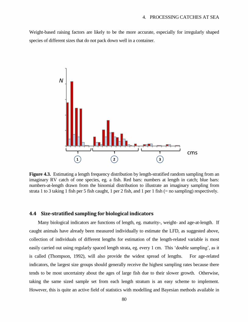
4. PROCESSING CATCHES AT SEA

80

Weight-based raising factors are likely to be the more accurate, especially for irregularly shaped

species of different sizes that do not pack down well in a container.

Figure 4.3. Estimating a length frequency distribution by length-stratified random sampling from an

imaginary RV catch of one species, eg. a fish. Red bars: numbers at length in catch; blue bars:

numbers-at-length drawn from the binomial distribution to illustrate an imaginary sampling from

strata 1 to 3 taking 1 fish per 5 fish caught, 1 per 2 fish, and 1 per 1 fish (= no sampling) respectively.

4.4 Size-stratified sampling for biological indicators

Many biological indicators are functions of length, eg. maturity-, weight- and age-at-length. If

caught animals have already been measured individually to estimate the LFD, as suggested above,

collection of individuals of different lengths for estimation of the length-related variable is most

easily carried out using regularly spaced length strata, eg. every 1 cm. This „double sampling‟, as it

is called (Thompson, 1992), will also provide the widest spread of lengths. For age-related

indicators, the largest size groups should generally receive the highest sampling rates because there

tends to be most uncertainty about the ages of large fish due to their slower growth. Otherwise,

taking the same sized sample set from each length stratum is an easy scheme to implement.

However, this is quite an active field of statistics with modelling and Bayesian methods available in

N

cms1 2 3

4. PROCESSING CATCHES AT SEA

81

connection with market sampling of commercial landings (see references in Cotter and Pilling,

2007).

Record keeping at all stages of catch processing should maintain the links between different

indicators or measures and the individual fish or samples of fish on which they were measured. The

links are important for raising factors, for checking back where a sample came from, as well as for

correlation studies and modelling.

4.5 Conclusions

The processing of catches on an ecosystem survey, whether from the main trawl or some other

catching device must be planned to suit the resources of space, time, and scientific crew available.

Formal catch-processing protocols are essential for every gear. They should cover the separation of

litter, rocks and other debris, sorting into species including rarities and confusables, size stratification

options, and the drawing of animals at random for unbiased estimation of indicators. A maximum

catch-sampling volume (MCSV) is proposed for when catches are too large to be searched

throughout for occurrences of rare species or size groups of a species. Scientific crew should be

trained in taxonomy and tested before being authorized to make identifications at sea since poor

identifications cannot be verified later and could seriously undermine an EMS. Protocols should

specify and name in a standard way any restricted identifications that are acceptable (eg. to genus or

family level). Procedures should be described for estimating quantities of difficult-to-separate

species, and for naming groups of unseparated mixed species. Catch samples for size- or age-related

indicators are most easily drawn using the length strata created when the length frequency

distribution is estimated. This should provide a reasonably constant coefficient of variation across

the size groups, though higher sampling rates in the larger groups may be advisable for some

indicators because of the wider range of ages among larger individuals.

5. WHICH INDICATORS?

82

5 WHICH INDICATORS?

Potentially, hundreds of indicators can be calculated from an EMS but presenting results for all

of them to an EAF management committee could provoke confusion. The best selection will be

linked to the high-level goals of the committee and the general and operational objectives (GOs and

OOs) developed from them for each ecosystem component or unit of concern (Hobday et al., 2007),

as schematized in Figure 1.1, page 17. For example, management may wish to prioritize foodweb

structure, protection of TEP species or, more pragmatically, to maintain the economic and social

benefits of fisheries. These must be translated by scientists into OOs for each species or component

of concern, then matched to informative indicators that can feasibly be monitored by an EMS or

other means, and compared with performance criteria thought to signal successful management

(Fletcher et al., 2005, Anonymous, 2011).

This section of the report provides three different groupings of RV ecosystem indicators. The

first is derived „bottom-up‟ from the logical sequence of catch processing tasks on an RV,

completion of which at every station will depend on resources of time and staff. The second and

third are „top-down‟ „wish-lists‟ for monitoring the effects of fishing, and for monitoring and

building up knowledge about the ecosystem generally. Managers of the EMS have the challenging

role of selecting what is feasible from what is desirable.

5.1 Indicators from different levels of catch processing

The stage of catch processing that can be consistently achieved for each catching device

deployed by an EMS may exert a strong influence on the number and types of indicator available.

One scientist working on a small, lively trawler might be expected to produce species lists for every

fished station and not much more, whereas a team of scientists on a large RV could produce species

lists, length-frequency distributions, and several other biological indicators for a range of species

from different catching devices. This subsection discusses feasibility and informativeness of catch-

based indicators according to stages of catch processing. A sequence of catch processing varying by

species according to priorities set by the EAF committee is schematized in Figure 5.1.

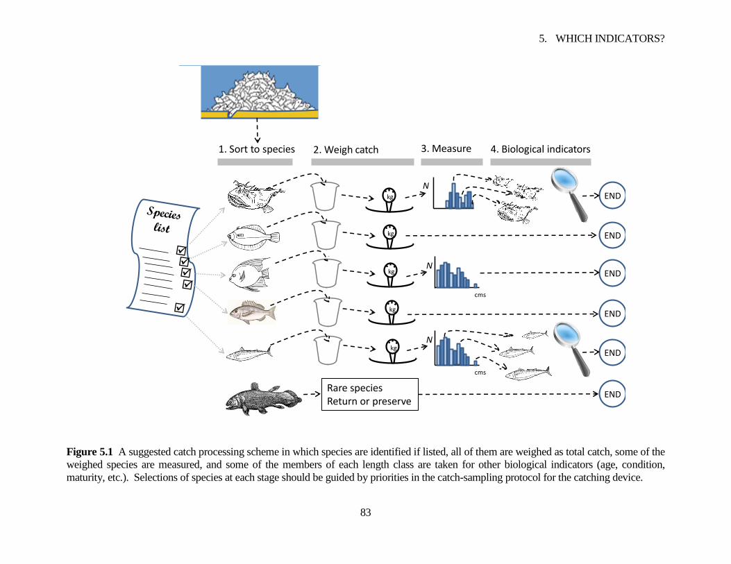
5. WHICH INDICATORS?

83

Figure 5.1 A suggested catch processing scheme in which species are identified if listed, all of them are weighed as total catch, some of the

weighed species are measured, and some of the members of each length class are taken for other biological indicators (age, condition,

maturity, etc.). Selections of species at each stage should be guided by priorities in the catch-sampling protocol for the catching device.

kg

kg

kg

kg

kg

cms

N

N

cms

N

1. Sort to species 2. Weigh catch 3. Measure 4. Biological indicators

END

END

END

END

END

ENDRare speciesReturn or preserve

5. WHICH INDICATORS?

84

5.1.1 Indicators from species lists

The simplest processing of catches taken on an EMS should, at the least, provide lists of species

found at each station fished. As discussed in section 4.2, the species might be ticked on a list

intended to simplify identifications at sea, or they might include all species found and identified. For

epibenthic and benthic samplers, the number of species found and the time taken to sort them

depends strongly on the mesh size used to sieve the catches, e.g. 5 or 10 mm internally (Callaway et

al., 2002b), or finer for infaunal sampling using a grab (Schlacher and Wooldridge, 1996).

„Occupancies‟ (eg Cotter et al., 2008, eg Patten and Smith-Patten, 2011) are a type of indicator

estimable from species lists by station. The occupancy for a species within a region or stratum is

defined as the proportion, p, of stations fished there where at least one individual of that species is

found. Declining occupancies of a species over time may signal a regional extirpation problem, the

seriousness of which will depend on whether the species domain is only partially overlapped, or fully

enclosed by the survey domain (section 3.1). If the species has an important trophic role as, for

example, some pelagic species do in „wasp-waist‟ ecosystems (Bakun, 2006), declining occupancies

may indicate a developing change in the food web. Increasing occupancies could indicate a stock

recovery, an invasive species or, again, a changing foodweb. Either way, a clear change of a species‟

occupancy is a signal worth investigating for causes such as commercial fishing, climate, etc. See

5. WHICH INDICATORS?

85

Figure 5.2 for examples of occupancy trends measured from the North Sea. Notice that the

change of survey trawl type in 1992 did not strongly affect the series, suggesting an advantage of

occupancies over CPUE data for assessing declining presence. Box 5.1 describes a Bayesian method

for smoothing occupancies.

Occupancies can be developed into a multi-species indicator (Cotter et al., 2008). To maximize

sensitivity to changing presences of species, the measure should only be derived for species known to

have been caught in the first few years of a survey, or at other times of plenty. The index, referred to

here as the Bayesian occupancy index (BOI), for year y and for all , ,1s S included species is

,y y ssBOI p S .

It decreases from 1 to 0 as species are found at fewer and fewer stations. Note that sporadic rarities

have low ,y sp and so have relatively little influence on changing values. Also, that species trending

in different directions are confounded.

A survey-based indicator comparable in some ways to the BOI except that it is based on CPUEs

is the threat indicator for marine fish (Dulvy et al., 2006). It was designed for assessing extinction

risk in relation to IUCN criteria. Dulvy et al (2006) estimated the threat index for a selected group of

species with known vulnerabilities to fishing or other environmental factors. The same approach

would aid interpretation of the BOI.

Related to occupancies is the spatial indicator called „positive area‟ (Woillez et al., 2009). The

„area of influence‟ around a station is the area made up of points in space that are closer to the station

than to any others. The positive area is the sum of the presence at each station weighted by area of

influence. Positive area can be plotted geographically and, for some applications, may be preferred

to the occupancy.

Species richness (number of species) is another possible indicator for species lists produced by

ecosystem surveys. However, it loses information about the geographic distributions of species,

implying that it is less informative about changes to an ecosystem. Richness is, nevertheless, a

widely used measure of biodiversity.

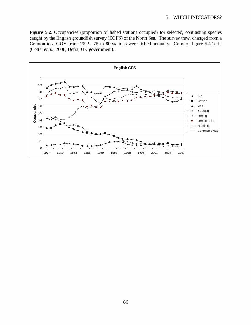
5. WHICH INDICATORS?

86

Figure 5.2. Occupancies (proportion of fished stations occupied) for selected, contrasting species

caught by the English groundfish survey (EGFS) of the North Sea. The survey trawl changed from a

Granton to a GOV from 1992. 75 to 80 stations were fished annually. Copy of figure 5.4.1c in

(Cotter et al., 2008, Defra, UK government).

English GFS

0

0.1

0.2

0.3

0.4

0.5

0.6

0.7

0.8

0.9

1

1977 1980 1983 1986 1989 1992 1995 1998 2001 2004 2007

Occu

pan

cie

s

Bib

Catfish

Cod

Spurdog

herring

Lemon sole

Haddock

Common skate

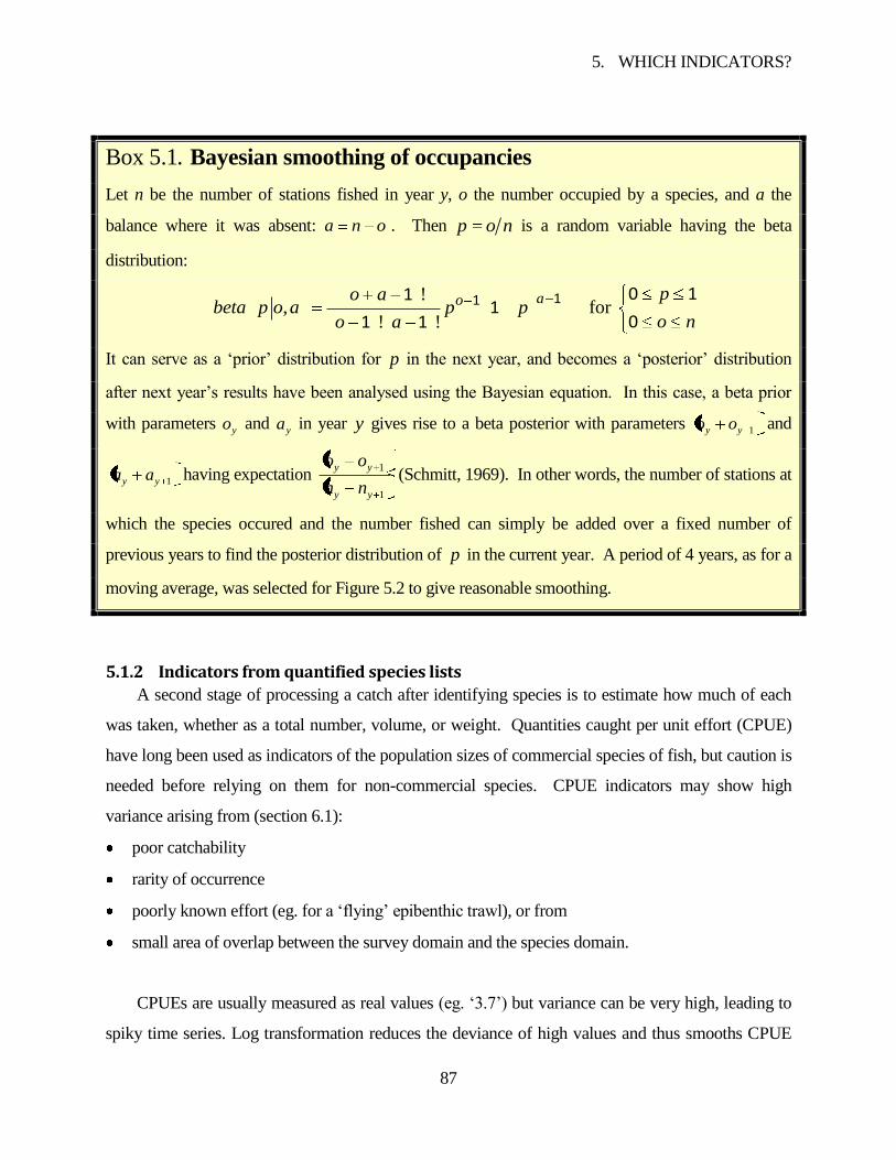
5. WHICH INDICATORS?

87

Box 5.1. Bayesian smoothing of occupancies

Let n be the number of stations fished in year y, o the number occupied by a species, and a the

balance where it was absent: ona . Then p o n is a random variable having the beta

distribution:

!

, for ! !

11 0 111

01 1

ao po abeta p o a p p

o no a

It can serve as a „prior‟ distribution for p in the next year, and becomes a „posterior‟ distribution

after next year‟s results have been analysed using the Bayesian equation. In this case, a beta prior

with parameters yo and ya in year y gives rise to a beta posterior with parameters 1yy oo and

1yy aa having expectation 1

1

yy

yy

nn

oo (Schmitt, 1969). In other words, the number of stations at

which the species occured and the number fished can simply be added over a fixed number of

previous years to find the posterior distribution of p in the current year. A period of 4 years, as for a

moving average, was selected for Figure 5.2 to give reasonable smoothing.

5.1.2 Indicators from quantified species lists

A second stage of processing a catch after identifying species is to estimate how much of each

was taken, whether as a total number, volume, or weight. Quantities caught per unit effort (CPUE)

have long been used as indicators of the population sizes of commercial species of fish, but caution is

needed before relying on them for non-commercial species. CPUE indicators may show high

variance arising from (section 6.1):

poor catchability

rarity of occurrence

poorly known effort (eg. for a „flying‟ epibenthic trawl), or from

small area of overlap between the survey domain and the species domain.

CPUEs are usually measured as real values (eg. „3.7‟) but variance can be very high, leading to

spiky time series. Log transformation reduces the deviance of high values and thus smooths CPUE

5. WHICH INDICATORS?

88

time series. A constant must be added to allow logs of any zero CPUEs occurring. The size of the

constant is arbitrary and affects the apparent variance of the log series. Zeros could be omitted by

defining CPUE as „given that one or more fish were caught‟ as for the mean-over-fish, section 3.4.

Another solution would be to down-grade CPUEs from real values to ordered categorical values after

division of catch by effort. Examples are „Lo, Med, Hi‟, or logarithmic bins: „0 – 3‟, „3.1 – 10‟, ‟10.1

– 30‟, etc. Ordered categorical CPUEs are expected to show more stable regional averages than real-

valued CPUEs because they smooth out exceptionally large values and high variance. However,

results become dependent on the bin sizes used. Yet another smoothing technique for CPUE time

series is Lotka‟s intrinsic population growth rate, ie. the slope of the trend line fitted to a time series

of log abundance indices. Advantages and disadvantages are discussed by Cotter et al. (2009).

Various spatial indicators, such as those listed in

5. WHICH INDICATORS?

89

Table 5.1 (Woillez et al., 2009), may aid interpretation of CPUEs by analysis of variation

spatially. By using them, responses to effects of fishing and other factors can be reduced to small

sets of indicator values relating to specific aspects of the geographic distributions. Some spatial

indicators are themselves amenable to multivariate analyses (e.g. Petitgas and Poulard, 2009). The

tabulated spatial indicators are insensitive to zero values and thus are unaffected by stations outside

the species domain. One, the global index of co-location, might be appropriate for measuring the

spatial distinctness between the domain of a species and that of a fishery characterized by spatial

effort data. This might help an assessment of the potential effect of the fishery on the species.

The main problem with CPUE time series in an EMS is that there are too many to interpret

consistently. Multivariate statistical methods such as principle components analysis (PCA) (Jackson,

2003) may allow the number of time series to be reduced to only 2 or 3; most sampling variation will

be found in the higher PCs. A more direct approach is to subset the CPUE series of different species

a priori according to the responses they are expected to show to fishing or other factors of interest, as

suggested by Dulvy et al. (2006) in connection with their threat indicator. This should improve the

uniformity of responses, making results easier to interpret. Informative groupings might be related to

direct effects of fishing, or to trophic roles eg. as top predators, planktotrophs, etc. Stable,

interpretable groupings of CPUE series, each group revealing different aspects of ecosystem

functioning, could serve conveniently to communicate key results from an RV ecosystem survey.

Modelling is another way of handling multiple CPUE series. A few examples from the many

published are trophic models (Cury et al., 2000, Christensen and Walters, 2004, Dunne and

Williams, 2009), size-based models (Shin and Cury, 2004, Shin et al., 2005, Pope et al., 2006,

Andersen and Pedersen, 2010, Barnes et al., 2010), and benthic models (Hiddink et al., 2006a). A

general problem with such models, as for some multivariate analyses, is that pre-requisite

assumptions may be difficult to defend in a compliance-monitoring situation, though they may be

acceptable for research. Other comments on modelling real data can be found in section 6.3.4.

Multispecies CPUEs can be used for calculating diversity indices relating to communities.

However, these summarizing statistics will be strongly affected by variable selectivities and

catchabilities for different species (sections 6.1.1, 6.1.2), and they lose the links between stations and

species‟ identities. They may therefore be poorly sensitive to effects of fishing or other factors.

Multispecies CPUEs can also be used in conjunction with data on trophic level of each species to

5. WHICH INDICATORS?

90

estimate the „marine trophic index‟ (MTI) (Pauly and Watson, 2005) but investigations have not

supported its use with RV surveys because of (i) the small range of trophic levels encountered by a

single trawl type, (ii) the relatively small number of stations fished compared with commercial

fisheries (for which the MTI was designed), and (iii) difficulties estimating trophic levels, some of

which need substantial adjustments for fish size (Jennings et al., 2002a, Cotter et al., 2008, Branch et

al., 2010). Stable isotope analyses and size-based indicators appear to be better tools for

investigating trophic relationships from RV surveys (eg. Jennings et al., 2002b). The threat indicator

of Dulvy et al. (2006) is another method for multispecies CPUEs. It estimates extinction risks.

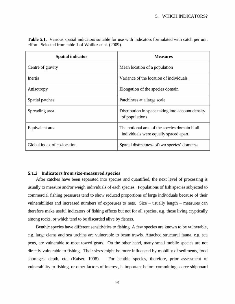
5. WHICH INDICATORS?

91

Table 5.1. Various spatial indicators suitable for use with indicators formulated with catch per unit

effort. Selected from table 1 of Woillez et al. (2009).

Spatial indicator Measures

Centre of gravity Mean location of a population

Inertia Variance of the location of individuals

Anisotropy Elongation of the species domain

Spatial patches Patchiness at a large scale

Spreading area Distribution in space taking into account density

of populations

Equivalent area The notional area of the species domain if all

individuals were equally spaced apart.

Global index of co-location Spatial distinctness of two species‟ domains

5.1.3 Indicators from size-measured species

After catches have been separated into species and quantified, the next level of processing is

usually to measure and/or weigh individuals of each species. Populations of fish species subjected to

commercial fishing pressures tend to show reduced proportions of large individuals because of their

vulnerabilities and increased numbers of exposures to nets. Size – usually length – measures can

therefore make useful indicators of fishing effects but not for all species, e.g. those living cryptically

among rocks, or which tend to be discarded alive by fishers.

Benthic species have different sensitivities to fishing. A few species are known to be vulnerable,

e.g. large clams and sea urchins are vulnerable to beam trawls. Attached structural fauna, e.g. sea

pens, are vulnerable to most towed gears. On the other hand, many small mobile species are not

directly vulnerable to fishing. Their sizes might be more influenced by mobility of sediments, food

shortages, depth, etc. (Kaiser, 1998). For benthic species, therefore, prior assessment of

vulnerability to fishing, or other factors of interest, is important before committing scarce shipboard

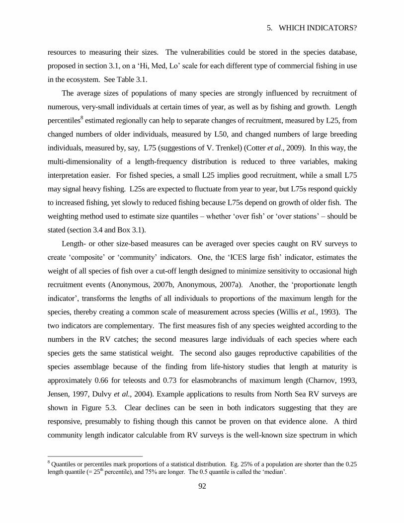
5. WHICH INDICATORS?

92

resources to measuring their sizes. The vulnerabilities could be stored in the species database,

proposed in section 3.1, on a „Hi, Med, Lo‟ scale for each different type of commercial fishing in use

in the ecosystem. See Table 3.1.

The average sizes of populations of many species are strongly influenced by recruitment of

numerous, very-small individuals at certain times of year, as well as by fishing and growth. Length

percentiles8 estimated regionally can help to separate changes of recruitment, measured by L25, from

changed numbers of older individuals, measured by L50, and changed numbers of large breeding

individuals, measured by, say, L75 (suggestions of V. Trenkel) (Cotter et al., 2009). In this way, the

multi-dimensionality of a length-frequency distribution is reduced to three variables, making

interpretation easier. For fished species, a small L25 implies good recruitment, while a small L75

may signal heavy fishing. L25s are expected to fluctuate from year to year, but L75s respond quickly

to increased fishing, yet slowly to reduced fishing because L75s depend on growth of older fish. The

weighting method used to estimate size quantiles – whether „over fish‟ or „over stations‟ – should be

stated (section 3.4 and Box 3.1).

Length- or other size-based measures can be averaged over species caught on RV surveys to

create „composite‟ or „community‟ indicators. One, the „ICES large fish‟ indicator, estimates the

weight of all species of fish over a cut-off length designed to minimize sensitivity to occasional high

recruitment events (Anonymous, 2007b, Anonymous, 2007a). Another, the „proportionate length

indicator‟, transforms the lengths of all individuals to proportions of the maximum length for the

species, thereby creating a common scale of measurement across species (Willis et al., 1993). The

two indicators are complementary. The first measures fish of any species weighted according to the

numbers in the RV catches; the second measures large individuals of each species where each

species gets the same statistical weight. The second also gauges reproductive capabilities of the

species assemblage because of the finding from life-history studies that length at maturity is

approximately 0.66 for teleosts and 0.73 for elasmobranchs of maximum length (Charnov, 1993,

Jensen, 1997, Dulvy et al., 2004). Example applications to results from North Sea RV surveys are

shown in Figure 5.3. Clear declines can be seen in both indicators suggesting that they are

responsive, presumably to fishing though this cannot be proven on that evidence alone. A third

community length indicator calculable from RV surveys is the well-known size spectrum in which

8 Quantiles or percentiles mark proportions of a statistical distribution. Eg. 25% of a population are shorter than the 0.25

length quantile (= 25th percentile), and 75% are longer. The 0.5 quantile is called the „median‟.

5. WHICH INDICATORS?

93

catches of all species are sorted into logarithmic length bins. Average CPUE tends to decline with

length and with greater steepness for heavily fished communities (Bianchi et al., 2000, Pope et al.,

2006). There are other community length indicators worth checking for applicability (Jennings and

Dulvy, 2005).

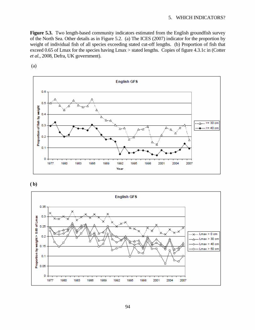
5. WHICH INDICATORS?

94

Figure 5.3. Two length-based community indicators estimated from the English groundfish survey

of the North Sea. Other details as in Figure 5.2. (a) The ICES (2007) indicator for the proportion by

weight of individual fish of all species exceeding stated cut-off lengths. (b) Proportion of fish that

exceed 0.65 of Lmax for the species having Lmax > stated lengths. Copies of figure 4.3.1c in (Cotter

et al., 2008, Defra, UK government).

(a)

( b)

5. WHICH INDICATORS?

95

5.1.4 Other biological indicators

When identification, quantification and measurement of a catch can be completed reliably for all

required species at every station, opportunities exist for estimating other biological indicators

although, since several are highly dependent on season, the EMS must be taking place in the correct

season. Fish or other animals might be sampled from quantified species groups (section 0) or from

the subsequently measured samples (section 5.1.3). Alternatively, whole groups could be used

without sampling. If sampled, bias with respect to size can be avoided either by stratifying by size or

by careful randomization (section 4.3). Sampling adds a component of variance to indicator values

but may be essential if there are many species to process and/or the chosen biological measures are

time-consuming to collect.

One informative biological measure is the weight of individuals of a species, obtainable if a

sensitive, motion-compensated balance is on board. Weight-at-length or „condition‟ can indicate

recent environmental conditions for growth. Low condition may imply too much competition for

available food and, perhaps, impaired reproductive capabilities (Shin et al., 2005, Cotter et al., 2009).

Key species of an ecosystem that are affected in this way would be worth investigating further, if

possible, since there may be an ecological link with fishing. Condition appears to be easier to

monitor than growth which would either require repeated surveys to sample clearly identifiable year

classes in the length frequency distribution, or tagging and weighing of individuals.

Age is only obtainable for some species caught on an EMS, though study of otoliths can

addtionally reveal information about stocks and migrations (Campana, 2005). Removal of otoliths,

scales, or other age-marked parts is a quick job for several species, but reading them requires time,

skill and, for many non-commercial species, some preliminary research to verify that visible rings do

indeed mark years or seasons. High demands for age reading could significantly delay publication of

results from an RV survey, so reasons for measuring many ages should be sound. Size-, weight-, and

maturity-at-age are all potentially informative indicators of how a species is faring. Relationships

discovered with year classes may indicate density-dependent effects on growth and reproduction.

Reproductive indicators measurable with RV surveys include indices of spawner abundance

(„SSN‟) and biomass („SSB‟); gonadosomatic index (GSI), and length- or age-at-maturity. GSI,

meaning gonad weight as a proportion of body weight, is the most sensitive to timing of the survey

relative to the spawning season of each species (Cotter et al., 2009) and therefore may only be

warranted for high-priority species meriting a specially-scheduled survey. SSN, SSB, and length- or

5. WHICH INDICATORS?

96

age-at-maturity should only be assessed when maturing of the gonad is clearly in evidence, usually in

the months just before breeding. Maturity of older individuals is usually easiest to assess, though

maturity staging in general, especially for non-commercial species, can be problematic especially

when different numbers of stages are defined by different authorities. Scientists making maturity

assessments should be trained, as for taxonomy. Age-at-maturity has been reported to decrease in

response to fishing, and young fish have been found to produce less viable eggs with shorter

spawning periods than older fish of some species (Trippel, 1995, Rochet et al., 2000, Trippel, 2003).

Length-at-maturity can be related to length quantiles to indicate the proportion of breeding adults in a

population. These findings support the relevance of reproductive indicators for EAF if they can be

measured on an an appropriately timed RV ecosystem survey. For further discussion of reproductive

indicators, see Kjesbu et al. (2003) and Witthames and Marshall (2008).

5.1.5 Conclusions

Selection of ecosystem indicators may have to allow for the gears being fished and practical

constraints on RV ecosystem surveys. Depending on facilities on board, catch processing generally

involves firstly, species identification, then quantification, then length measurements and, finally,

additional sampling for biological measures. Catch-based indicators can be graded to correspond to

these different levels of processing, and it does not necessarily follow that, because an EMS must use

only a small RV with small numbers of scientific crew, little useful information will be derived from

it.

Indicators for species lists include occupancies, spatial positive area, and the Bayesian

occupancy index (BOI). They appear to be particularly suitable for rare and poorly catchable

species. Species richness and diversity are not recommended as ecosystem indicators for monitoring

because they delete spatial information. Indicators for species whose total catch has been quantified

by weighing or counting are mostly CPUE-based though, for many non-commercial species, CPUEs

are likely to be poorly measured because of poor catchabilities and other reasons. A priori groupings

of species by expected sensitivities to fishing or other factors is important for reducing the number of

potentially confusing trends when examining CPUE time series. Intrinsic population growth rate,

spatial indicators, and multivariate techniques can smooth them and reduce their dimensionality. The

threat index assesses extinction risk from survey CPUEs. Modelling may also play a role providing

that pre-requisite assumptions are acceptable for formal monitoring purposes. Indicators not

recommended for RV CPUE series are richness, diversity, and mean trophic level.

5. WHICH INDICATORS?

97

Quantiles are recommended as indicators for species whose sizes – usually lengths – have been

measured. The L25, L50, and L75 (or other) quantiles can be used to reduce the multi-

dimensionality of length-frequency distributions while still distinguishing abundant recruiting classes

from newly mature animals and older broodstock. Size may not be worth measuring for species not

subjected to size-selection by commercial fishing gear. Sizes can be used to create composite

community indicators that have been shown to vary over time, probably as a result of fishing.

Indicators of biological functioning tend to be highly vulnerable to bias from the season of the

survey, and are sensitive to unintentionally size-selective sampling of catches. Weight-at-length or

bodily condition can indicate growing conditions and perhaps density-dependent effects of strong

year classes. Poor condition is of concern because it implies poor reproductive capabilities. Age

determinations require time, skill, and verification, and could delay publication of RV survey results.

Reproductive indicators like SSN and SSB should only be assessed by RV surveys occurring in the

months just before spawning. Other reproductive indicators like GSI are even more sensitive to

season. Length- or age-at-maturity is useful for estimating breeding proportions in a population and

thus may be useful indicators of the long-term security of a species.

A summary of a suggested 4-level hierarchy of catch measures for demersal trawling with

different RV resources is shown in Table 5.2. It ranges from identifying and quantifying a standard

list of species as the first priority, to measuring all species and disecting some of them for age- and

maturity-related indicators. A summary of a suggested hierarchy for epibenthic beam trawling or

dredging is shown in Table 5.3. A hierarchy of feasible infaunal sampling could also look like Table

5.3 but with smaller mesh sizes, e.g. 2 and 1 mm instead of 10 and 5 mm.

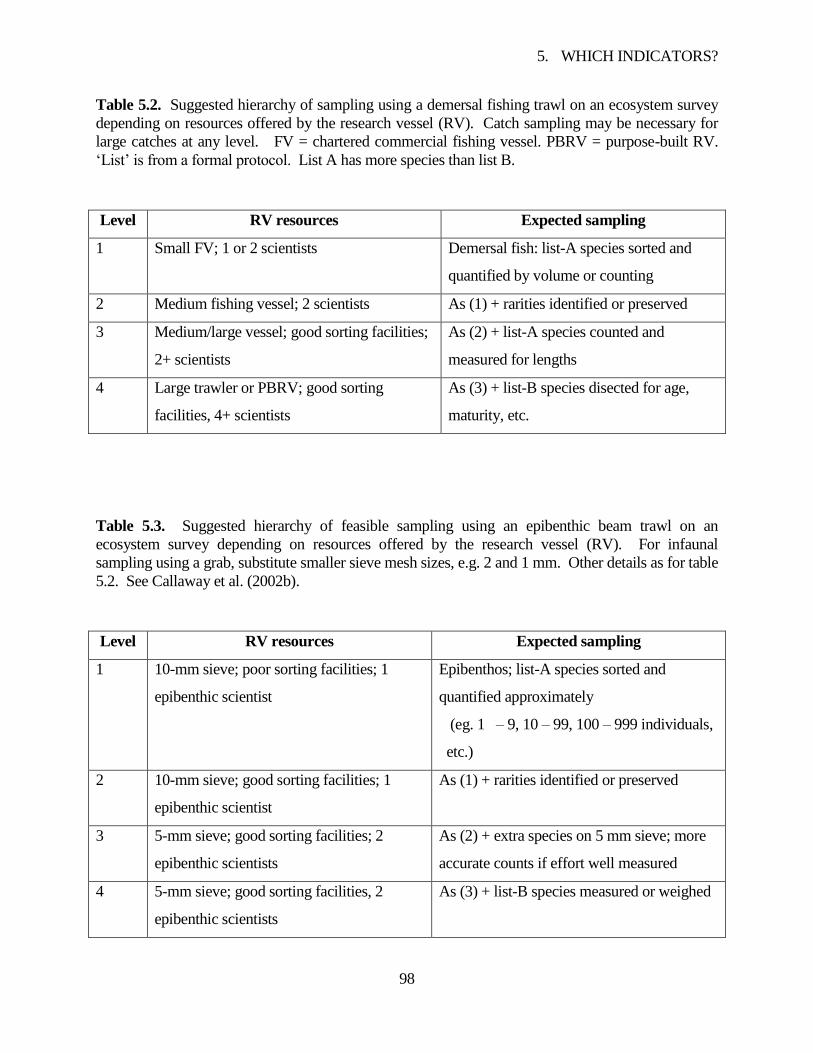
5. WHICH INDICATORS?

98

Table 5.2. Suggested hierarchy of sampling using a demersal fishing trawl on an ecosystem survey

depending on resources offered by the research vessel (RV). Catch sampling may be necessary for

large catches at any level. FV = chartered commercial fishing vessel. PBRV = purpose-built RV.

„List‟ is from a formal protocol. List A has more species than list B.

Level RV resources Expected sampling

1 Small FV; 1 or 2 scientists Demersal fish: list-A species sorted and

quantified by volume or counting

2 Medium fishing vessel; 2 scientists As (1) + rarities identified or preserved

3 Medium/large vessel; good sorting facilities;

2+ scientists

As (2) + list-A species counted and

measured for lengths

4 Large trawler or PBRV; good sorting

facilities, 4+ scientists

As (3) + list-B species disected for age,

maturity, etc.

Table 5.3. Suggested hierarchy of feasible sampling using an epibenthic beam trawl on an

ecosystem survey depending on resources offered by the research vessel (RV). For infaunal

sampling using a grab, substitute smaller sieve mesh sizes, e.g. 2 and 1 mm. Other details as for table

5.2. See Callaway et al. (2002b).

Level RV resources Expected sampling

1 10-mm sieve; poor sorting facilities; 1

epibenthic scientist

Epibenthos; list-A species sorted and

quantified approximately

(eg. 1 – 9, 10 – 99, 100 – 999 individuals,

etc.)

2 10-mm sieve; good sorting facilities; 1

epibenthic scientist

As (1) + rarities identified or preserved

3 5-mm sieve; good sorting facilities; 2

epibenthic scientists

As (2) + extra species on 5 mm sieve; more

accurate counts if effort well measured

4 5-mm sieve; good sorting facilities, 2

epibenthic scientists

As (3) + list-B species measured or weighed

5. WHICH INDICATORS?

99

5.2 Indicators for monitoring effects of fishing

Table 5.4 is intended to assist the selection of indicators and groupings of sensitive ecosystem

components for monitoring and managing the impacts of commercial fisheries. Several notes, linked

by superscript numbers to entries in the table, are meant to amplify the abbreviated contents of the

table. The term „parameter‟ is used for naming properties of ecosystem components thought to have

a true but unknown value for a population in an ecosystem at a given time. Then, by analogy with

the same terms in Statistics, the indicator is an estimator for the parameter. Values of the indicator

should be proportional to or, at least, show a monotonic relationship with values of the parameter.

Sources of data other than RV surveys exist for calculation of several indicators. These are noted in

the last column of the table but without any assessment of their relative merits; they would depend on

local circumstances.

Table 5.4 was prepared from the output of the FAO expert committee referred to in the

Acknowledgements.

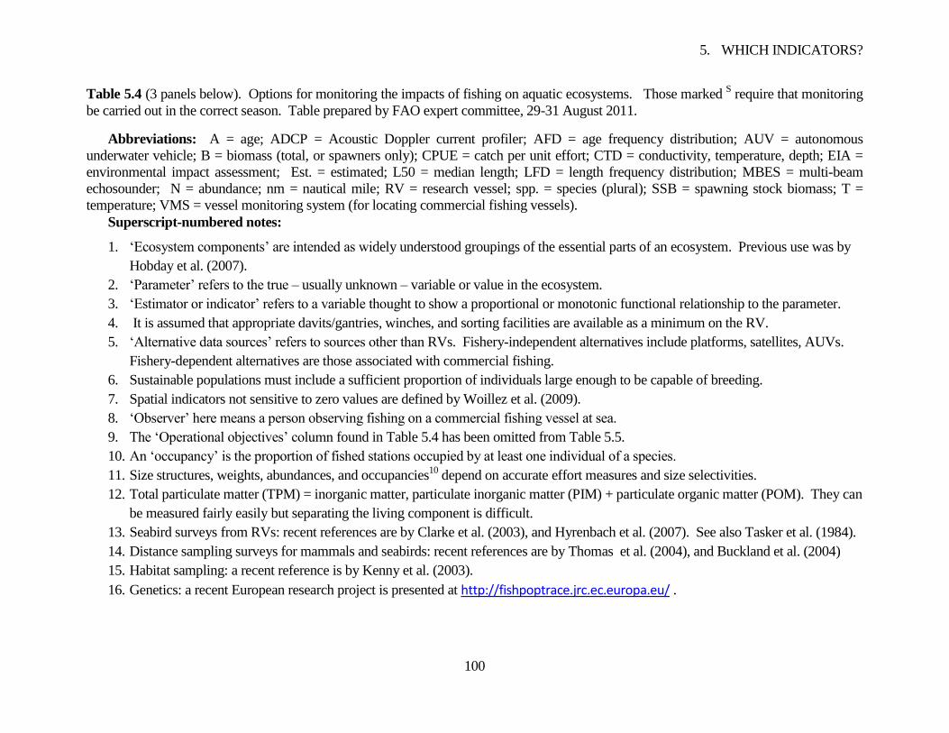
5. WHICH INDICATORS?

100

Table 5.4 (3 panels below). Options for monitoring the impacts of fishing on aquatic ecosystems. Those marked S require that monitoring

be carried out in the correct season. Table prepared by FAO expert committee, 29-31 August 2011.

Abbreviations: A = age; ADCP = Acoustic Doppler current profiler; AFD = age frequency distribution; AUV = autonomous

underwater vehicle; B = biomass (total, or spawners only); CPUE = catch per unit effort; CTD = conductivity, temperature, depth; EIA =

environmental impact assessment; Est. = estimated; L50 = median length; LFD = length frequency distribution; MBES = multi-beam

echosounder; N = abundance; nm = nautical mile; RV = research vessel; spp. = species (plural); SSB = spawning stock biomass; T =

temperature; VMS = vessel monitoring system (for locating commercial fishing vessels).

Superscript-numbered notes:

1. „Ecosystem components‟ are intended as widely understood groupings of the essential parts of an ecosystem. Previous use was by

Hobday et al. (2007).

2. „Parameter‟ refers to the true – usually unknown – variable or value in the ecosystem.

3. „Estimator or indicator‟ refers to a variable thought to show a proportional or monotonic functional relationship to the parameter.

4. It is assumed that appropriate davits/gantries, winches, and sorting facilities are available as a minimum on the RV.

5. „Alternative data sources‟ refers to sources other than RVs. Fishery-independent alternatives include platforms, satellites, AUVs.

Fishery-dependent alternatives are those associated with commercial fishing.

6. Sustainable populations must include a sufficient proportion of individuals large enough to be capable of breeding.

7. Spatial indicators not sensitive to zero values are defined by Woillez et al. (2009).

8. „Observer‟ here means a person observing fishing on a commercial fishing vessel at sea.

9. The „Operational objectives‟ column found in Table 5.4 has been omitted from Table 5.5.

10. An „occupancy‟ is the proportion of fished stations occupied by at least one individual of a species.

11. Size structures, weights, abundances, and occupancies10

depend on accurate effort measures and size selectivities.

12. Total particulate matter (TPM) = inorganic matter, particulate inorganic matter (PIM) + particulate organic matter (POM). They can

be measured fairly easily but separating the living component is difficult.

13. Seabird surveys from RVs: recent references are by Clarke et al. (2003), and Hyrenbach et al. (2007). See also Tasker et al. (1984).

14. Distance sampling surveys for mammals and seabirds: recent references are by Thomas et al. (2004), and Buckland et al. (2004)

15. Habitat sampling: a recent reference is by Kenny et al. (2003).

16. Genetics: a recent European research project is presented at http://fishpoptrace.jrc.ec.europa.eu/ .

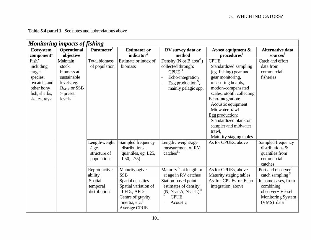
5. WHICH INDICATORS?

101

Table 5.4 panel 1. See notes and abbreviations above

Monitoring impacts of fishing Ecosystem

component1

Operational

objective

Parameter2

Estimator or

indicator3

RV survey data or

method

At-sea equipment &

procedures4

Alternative data

sources5

„Fish‟

including

target

species,

bycatch, and

other bony

fish, sharks,

skates, rays

Maintain

stock

biomass at

sustainable

levels, eg.

BMSY or SSB

> preset

levels

Total biomass

of population

Estimate or index of

biomass

Density (N or B.area-1

)

collected through:

- CPUE11

- Echo-integration

- Egg production S

,

mainly pelagic spp.

CPUE:

Standardized sampling

(eg. fishing) gear and

gear monitoring,

measuring boards,

motion-compensated

scales, otolith collecting

Echo-integration:

Acoustic equipment

Midwater trawl

Egg production:

Standardized plankton

sampler and midwater

trawl,

Maturity-staging tables

Catch and effort

data from

commercial

fisheries

Length/weight

/age

structure of

population6

Sampled frequency

distributions,

quantiles, eg. L25,

L50, L75)

Length / weight/age

measurement of RV

catches11

As for CPUEs, above Sampled frequency

distributions &

quantiles from

commercial

catches

Reproductive

ability

Maturity ogive

SSB

Maturity S

at length or

at age in RV catches

As for CPUEs, above

Maturity staging tables

Port and observer8

catch sampling S

Spatial-

temporal

distribution

Spatial densities

Spatial variation of

LFDs, AFDs

Centre of gravity

inertia, etc.7

Average CPUE

Station-based point

estimates of density

(N, N-at-A, N-at-L)11

- CPUE

- Acoustic

As for CPUEs or Echo-

integration, above

In some cases, from

combining

observer+ Vessel

Monitoring System

(VMS) data

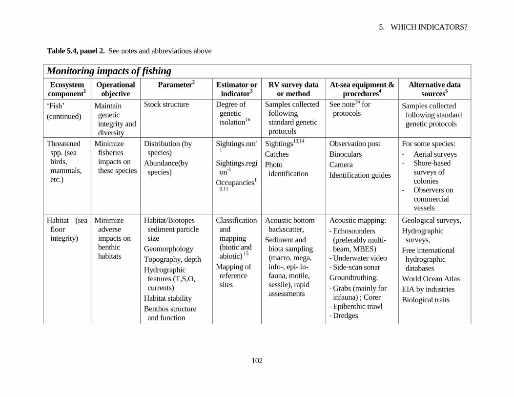
5. WHICH INDICATORS?

102

Table 5.4, panel 2. See notes and abbreviations above

Monitoring impacts of fishing

Ecosystem

component1

Operational

objective

Parameter2

Estimator or

indicator3

RV survey data

or method

At-sea equipment &

procedures4

Alternative data

sources5

„Fish‟

(continued)

Maintain

genetic

integrity and

diversity

Stock structure Degree of

genetic

isolation16

Samples collected

following

standard genetic

protocols

See note16

for

protocols Samples collected

following standard

genetic protocols

Threatened

spp. (sea

birds,

mammals,

etc.)

Minimize

fisheries

impacts on

these species

Distribution (by

species)

Abundance(by

species)

Sightings.nm-

1

Sightings.regi

on-1

Occupancies1

0,11

Sightings13,14

Catches

Photo

identification

Observation post

Binoculars

Camera

Identification guides

For some species:

- Aerial surveys

- Shore-based

surveys of

colonies

- Observers on

commercial

vessels

Habitat (sea

floor

integrity)

Minimize

adverse

impacts on

benthic

habitats

Habitat/Biotopes

sediment particle

size

Geomorphology

Topography, depth

Hydrographic

features (T,S,O,

currents)

Habitat stability

Benthos structure

and function

Classification

and

mapping

(biotic and

abiotic) 15

Mapping of

reference

sites

Acoustic bottom

backscatter,

Sediment and

biota sampling

(macro, mega,

info-, epi- in-

fauna, motile,

sessile), rapid

assessments

Acoustic mapping:

- Echosounders

(preferably multi-

beam, MBES)

- Underwater video

- Side-scan sonar

Groundtruthing:

- Grabs (mainly for

infauna) ; Corer

- Epibenthic trawl

- Dredges

Geological surveys,

Hydrographic

surveys,

Free international

hydrographic

databases

World Ocean Atlas

EIA by industries

Biological traits

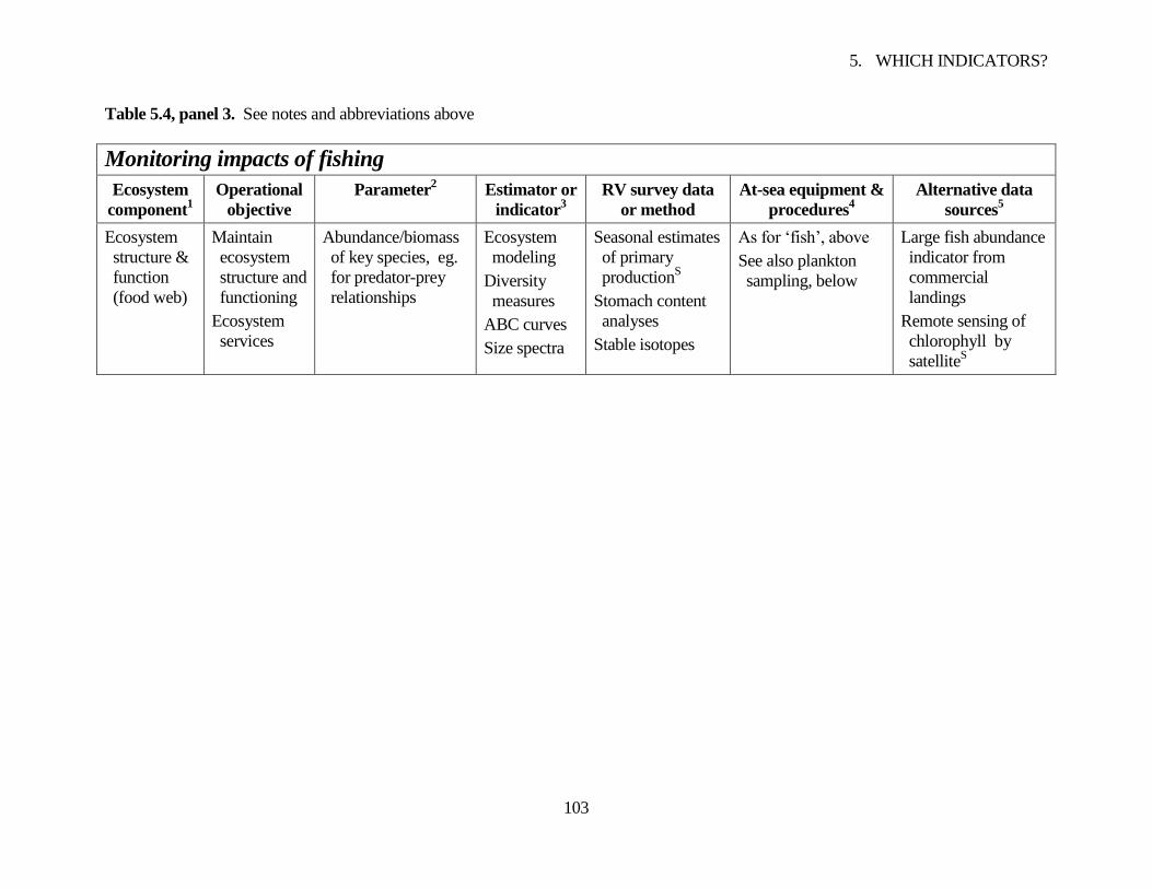
5. WHICH INDICATORS?

103

Table 5.4, panel 3. See notes and abbreviations above

Monitoring impacts of fishing

Ecosystem

component1

Operational

objective

Parameter2

Estimator or

indicator3

RV survey data

or method

At-sea equipment &

procedures4

Alternative data

sources5

Ecosystem

structure &

function

(food web)

Maintain

ecosystem

structure and

functioning

Ecosystem

services

Abundance/biomass

of key species, eg.

for predator-prey

relationships

Ecosystem

modeling

Diversity

measures

ABC curves

Size spectra

Seasonal estimates

of primary

productionS

Stomach content

analyses

Stable isotopes

As for „fish‟, above

See also plankton

sampling, below

Large fish abundance

indicator from

commercial

landings

Remote sensing of

chlorophyll by

satelliteS

5. WHICH INDICATORS?

104

5.3 Indicators for monitoring the ecosystem

Table 5.5 is intended to assist growth of understanding of the ecosystem being fished, given an

initial characterization based on available knowledge (section 2.2). Improved understanding may

point to better fishing strategies for sustainability and improved yields, and to better management

policies and indicators. Operational objectives are omitted from the table because managerial

decisions are not expected in direct response to improving knowledge. Many ideas are listed. They

are meant to be options; monitoring all of them would not just require a large RV and crew but also

much time at sea at different seasons. Notes to the table are as for Table 5.4.

Table 5.5 was prepared from the output of the FAO expert committee referred to in the

Acknowledgements.

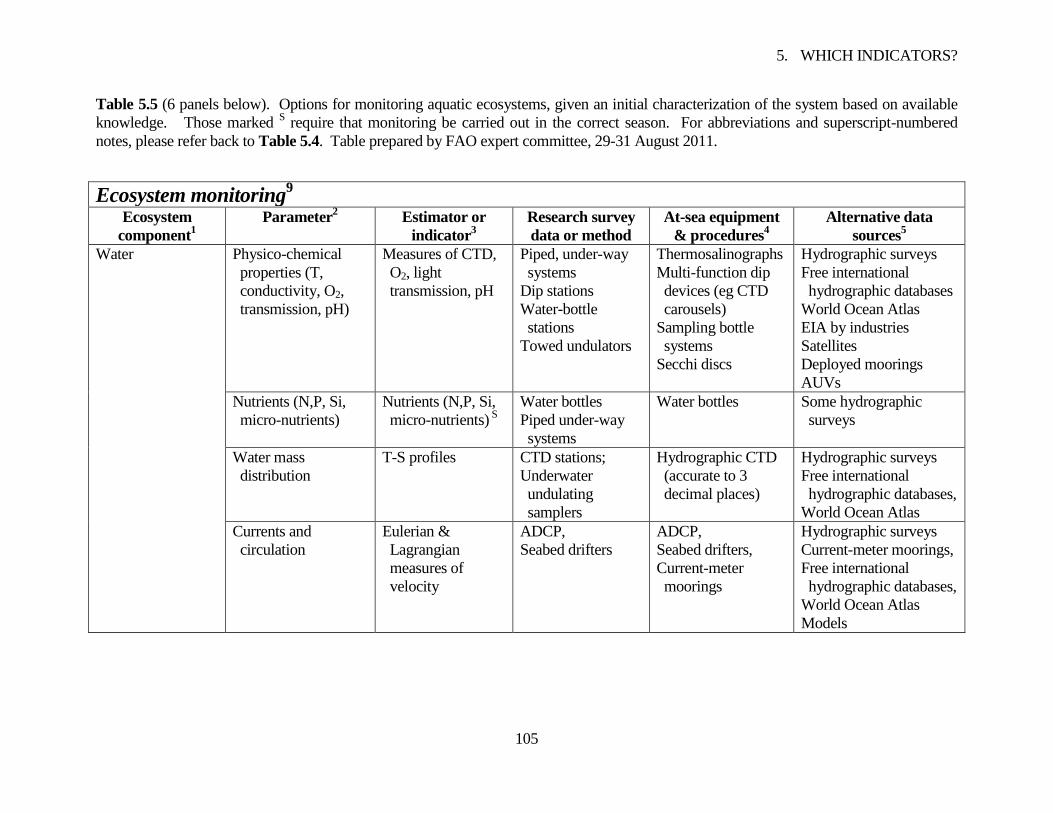
5. WHICH INDICATORS?

105

Table 5.5 (6 panels below). Options for monitoring aquatic ecosystems, given an initial characterization of the system based on available

knowledge. Those marked S require that monitoring be carried out in the correct season. For abbreviations and superscript-numbered

notes, please refer back to Table 5.4. Table prepared by FAO expert committee, 29-31 August 2011.

Ecosystem monitoring9

Ecosystem

component1

Parameter2

Estimator or

indicator3

Research survey

data or method

At-sea equipment

& procedures4

Alternative data

sources5

Water Physico-chemical

properties (T,

conductivity, O2,

transmission, pH)

Measures of CTD,

O2, light

transmission, pH

Piped, under-way

systems

Dip stations

Water-bottle

stations

Towed undulators

Thermosalinographs

Multi-function dip

devices (eg CTD

carousels)

Sampling bottle

systems

Secchi discs

Hydrographic surveys

Free international

hydrographic databases

World Ocean Atlas

EIA by industries

Satellites

Deployed moorings

AUVs

Nutrients (N,P, Si,

micro-nutrients)

Nutrients (N,P, Si,

micro-nutrients) S

Water bottles

Piped under-way

systems

Water bottles Some hydrographic

surveys

Water mass

distribution

T-S profiles CTD stations;

Underwater

undulating

samplers

Hydrographic CTD

(accurate to 3

decimal places)

Hydrographic surveys

Free international

hydrographic databases,

World Ocean Atlas

Currents and

circulation

Eulerian &

Lagrangian

measures of

velocity

ADCP,

Seabed drifters

ADCP,

Seabed drifters,

Current-meter

moorings

Hydrographic surveys

Current-meter moorings,

Free international

hydrographic databases,

World Ocean Atlas

Models

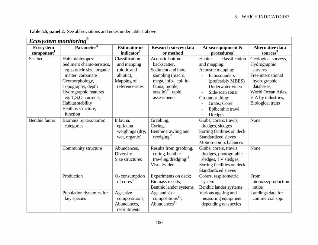
5. WHICH INDICATORS?

106

Table 5.5, panel 2. See abbreviations and notes under table 1 above

Ecosystem monitoring9

Ecosystem

component1

Parameter2

Estimator or

indicator3

Research survey data

or method

At-sea equipment &

procedures4

Alternative data

sources5

Sea bed Habitat/biotopes:

Sediment charac-teristics,

eg. particle size, organic

matter, carbonate

Geomorphology,

Topography, depth

Hydrographic features

eg. T,S,O, currents,

Habitat stability

Benthos structure,

function

Classification

and mapping

(biotic and

abiotic),

Mapping of

reference sites

Acoustic bottom

backscatter,

Sediment and biota

sampling (macro,

mega, info-, epi- in-

fauna, motile,

sessile)11

, rapid

assessments

Habitat classification

and mapping:

Acoustic mapping:

- Echosounders

(preferably MBES)

- Underwater video

- Side-scan sonar

Groundtruthing:

- Grabs; Corer

- Epibenthic trawl

- Dredges

Geological surveys,

Hydrographic

surveys

Free international

hydrographic

databases,

World Ocean Atlas,

EIA by industries,

Biological traits

Benthic fauna Biomass by taxonomic

categories

Infauna,

epifauna

weighings (dry,

wet, organic)

Grabbing,

Coring,

Benthic trawling and

dredging11

Grabs, corers, trawls,

dredges, sledges

Sorting facilities on deck

Standardized sieves

Motion-comp. balances

None

Community structure Abundances,

Diversity

Size structures

Results from grabbing,

coring, benthic

trawling/dredging11

Visual/video

Grabs, corers, trawls,

dredges, photographic

sledges, TV sledges;

Sorting facilities on deck

Standardized sieves

None

Production O2 consumption

of cores S

Experiments on deck;

Biomass results;

Benthic lander systems

Corers, respirometric

system

Benthic lander systems

From

biomass/production

ratios

Population dynamics for

key species

Age, size

compo-sitions;

Abundances,

recruitments

Age and size

compositions11

;

Abundances11

Various age-ing and

measuring equipment

depending on species

Landings data for

commercial spp.

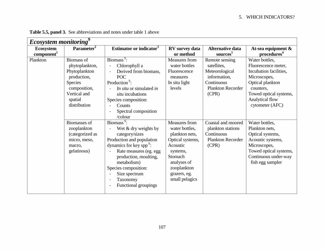
5. WHICH INDICATORS?

107

Table 5.5, panel 3. See abbreviations and notes under table 1 above

Ecosystem monitoring9

Ecosystem

component1

Parameter2

Estimator or indicator3

RV survey data

or method

Alternative data

sources5

At-sea equipment &

procedures4

Plankton Biomass of

phytoplankton,

Phytoplankton

production,

Species

composition,

Vertical and

spatial

distribution

Biomass S:

- Chlorophyll a

- Derived from biomass,

POC

Production S

:

- In situ or simulated in

situ incubations

Species composition:

- Counts

- Spectral composition

/colour

Measures from

water bottles

Fluorescence

measures

In situ light

levels

Remote sensing

satellites,

Meteorological

information,

Continuous

Plankton Recorder

(CPR)

Water bottles,

Fluorescence meter,

Incubation facilities,

Microscopes,

Optical plankton

counters,

Towed optical systems,

Analytical flow

cytometer (AFC)

Biomasses of

zooplankton

(categorized as

micro, meso,

macro,

gelatinous)

Biomass S:

- Wet & dry weights by

category/sizes

Production and population

dynamics for key spp S:

- Rate measures (eg. egg

production, moulting,

metabolism)

Species composition:

- Size spectrum

- Taxonomy

- Functional groupings

Measures from

water bottles,

plankton nets,

Optical systems,

Acoustic

systems,

Stomach

analyses of

zooplankton

grazers, eg.

small pelagics

Coastal and moored

plankton stations

Continuous

Plankton Recorder

(CPR)

Water bottles,

Plankton nets,

Optical systems,

Acoustic systems,

Microscopes,

Towed optical systems,

Continuous under-way

fish egg sampler

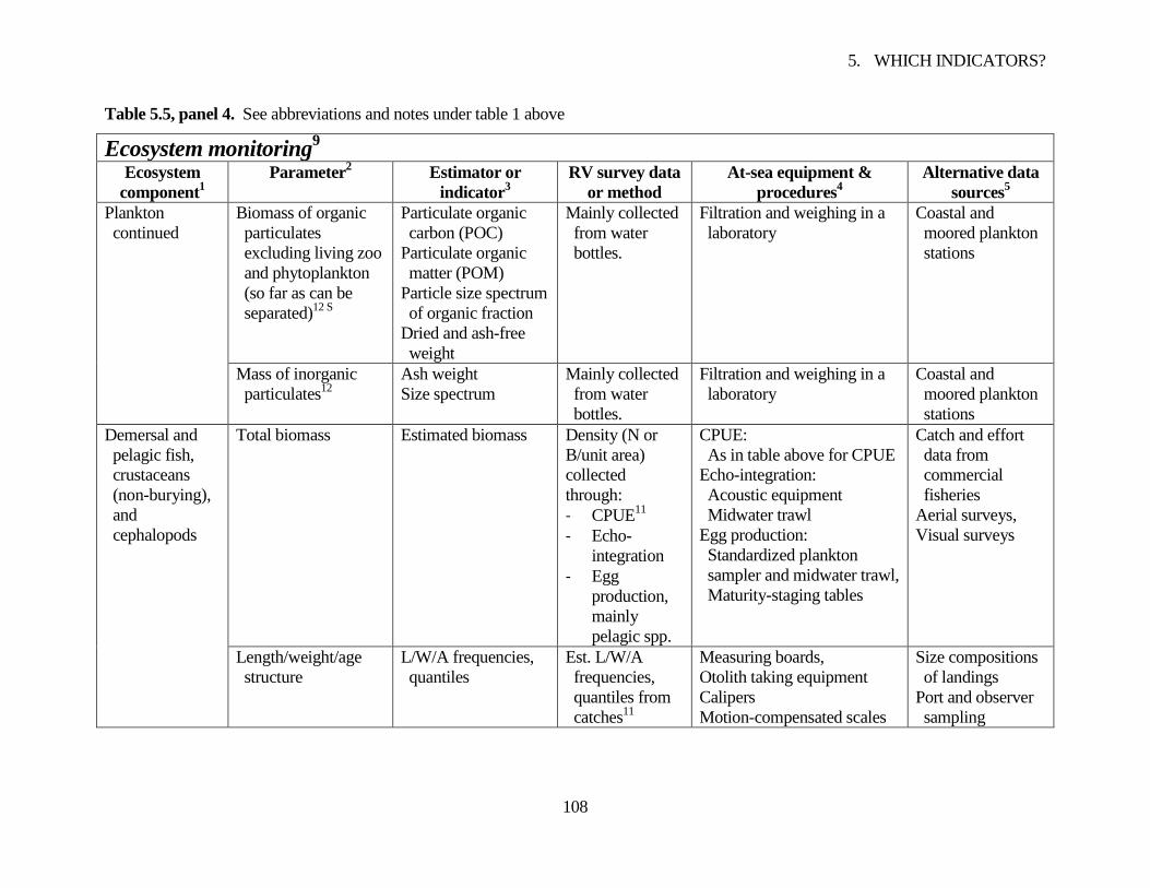
5. WHICH INDICATORS?

108

Table 5.5, panel 4. See abbreviations and notes under table 1 above

Ecosystem monitoring9

Ecosystem

component1

Parameter2

Estimator or

indicator3

RV survey data

or method

At-sea equipment &

procedures4

Alternative data

sources5

Plankton

continued Biomass of organic

particulates

excluding living zoo

and phytoplankton

(so far as can be

separated)12 S

Particulate organic

carbon (POC)

Particulate organic

matter (POM)

Particle size spectrum

of organic fraction

Dried and ash-free

weight

Mainly collected

from water

bottles.

Filtration and weighing in a

laboratory

Coastal and

moored plankton

stations

Mass of inorganic

particulates12

Ash weight

Size spectrum

Mainly collected

from water

bottles.

Filtration and weighing in a

laboratory

Coastal and

moored plankton

stations

Demersal and

pelagic fish,

crustaceans

(non-burying),

and

cephalopods

Total biomass Estimated biomass Density (N or

B/unit area)

collected

through:

- CPUE11

- Echo-

integration

- Egg

production,

mainly

pelagic spp.

CPUE:

As in table above for CPUE

Echo-integration:

Acoustic equipment

Midwater trawl

Egg production:

Standardized plankton

sampler and midwater trawl,

Maturity-staging tables

Catch and effort

data from

commercial

fisheries

Aerial surveys,

Visual surveys

Length/weight/age

structure

L/W/A frequencies,

quantiles

Est. L/W/A

frequencies,

quantiles from

catches11

Measuring boards,

Otolith taking equipment

Calipers

Motion-compensated scales

Size compositions

of landings

Port and observer

sampling

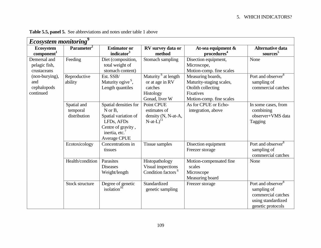
5. WHICH INDICATORS?

109

Table 5.5, panel 5. See abbreviations and notes under table 1 above

Ecosystem monitoring9

Ecosystem

component1

Parameter2

Estimator or

indicator3

RV survey data or

method

At-sea equipment &

procedures4

Alternative data

sources5

Demersal and

pelagic fish,

crustaceans

(non-burying),

and

cephalopods

continued

Feeding Diet (composition,

total weight of

stomach content)

Stomach sampling Disection equipment,

Microscope,

Motion-comp. fine scales

None

Reproductive

ability

Est. SSB/

Maturity ogive S

,

Length quantiles

Maturity S

at length

or at age in RV

catches

Histology

Gonad, liver W

Measuring boards,

Maturity-staging scales,

Otolith collecting

Fixatives

Motion-comp. fine scales

Port and observer8

sampling of

commercial catches

Spatial and

temporal

distribution

Spatial densities for

N or B,

Spatial variation of

LFDs, AFDs

Centre of gravity ,

inertia, etc.7

Average CPUE

Point CPUE

estimates of

density (N, N-at-A,

N-at-L)11

As for CPUE or Echo-

integration, above

In some cases, from

combining

observer+VMS data

Tagging

Ecotoxicology Concentrations in

tissues

Tissue samples

Disection equipment

Freezer storage

Port and observer8

sampling of

commercial catches

Health/condition Parasites

Diseases

Weight/length

Histopathology

Visual inspections

Condition factors S

Motion-compensated fine

scales

Microscope

Measuring board

None

Stock structure Degree of genetic

isolation16

Standardized

genetic sampling

Freezer storage Port and observer8

sampling of

commercial catches

using standardized

genetic protocols

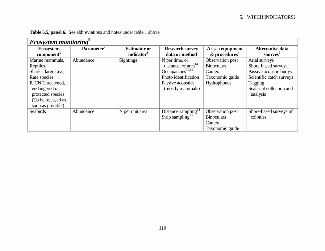
5. WHICH INDICATORS?

110

Table 5.5, panel 6. See abbreviations and notes under table 1 above

Ecosystem monitoring9

Ecosystem

component1

Parameter2

Estimator or

indicator3

Research survey

data or method

At-sea equipment

& procedures4

Alternative data

sources5

Marine mammals,

Reptiles,

Sharks, large rays,

Rare species

IUCN Threatened,

endangered or

protected species

(To be released as

soon as possible)

Abundance Sightings N per time, or

distance, or area14

Occupancies10,11

Photo identification

Passive acoustics

(mostly mammals)

Observation post

Binoculars

Camera

Taxonomic guide

Hydrophones

Arial surveys

Shore-based surveys

Passive acoustic buoys

Scientific catch surveys

Tagging

Seal scat collection and

analysis

Seabirds Abundance N per unit area Distance sampling14

Strip sampling13

Observation post

Binoculars

Camera

Taxonomic guide

Shore-based surveys of

colonies

6. ANALYSIS OF BIOLOGICAL DATA

111

6 ANALYSIS OF BIOLOGICAL DATA FROM AN ECOSYSTEM SURVEY

Physical and chemical oceanographic measures made on an RV ecosystem monitoring survey

(EMS) can be used for regional estimation of summarizing statistics (section 3.4) or they may be

collected in a database for modelling of oceanic and planktonic processes (Fox and Aldridge, 2008).

Groundfish surveys are typically analysed routinely by a fish stock working group considering one

species at a time. By contrast, the scope for statistical estimation and modelling of biological data

obtained from EMSs is wide, with no concensus yet available on what a routine analysis might

involve.

This section discusses the special problems of analysis posed by biological data derived from

EMSs. Firstly, practical and theoretical constraints on analyses are listed and ways forward

suggested. Secondly, statistical and modelling methods are very briefly discussed in relation to

different types of data, eg. presence-absence, ranked, real-valued. Monitoring of the habitat and

community components raises special issues that are discussed in two separate, additional sections.

6.1 Practical constraints on data analysis

This section lists some constraints on EMS data analysis posed by practical aspects of a survey.

6.1.1 Variable selectivities

Each catching gear in use on an EMS will exhibit different selectivities by size for different

species. Consequently, many indicators must be tied specifically to one type of catching gear so that

size-selectivity effects are constant, eg.

Multi-species indicators such as diversity and community measures

Size- and age-based indicators such as length-frequency distributions

Abundances that are greatly increased by small individuals.

Concerning the selectivity of trawls, large individuals that do not pass through the mesh are

often assumed to be 100% selected. However, the assumption may be invalid for species for which a

trawl was not designed, that habitually swim above the headline or below the footrope, or that are

strong enough to swim in front of the trawl. Some species are herded by a trawl, some not, a factor

that further affects selectivities. Other towed fishing gear can also exhibit size selectivity additional

to that of the mesh of the netting. The gear used to derive measured values that might be responsive

6. ANALYSIS OF BIOLOGICAL DATA

112

to size selectivity should always be stated. A few ecological measures may be relatively independent

of size-selectivity, eg. age-at-length, and maturity-at-age.

6.1.2 Low catchabilities

A species that is rarely seen on an EMS is either scarce or it is poorly caught. A low rate of

occurrence increases CVs of estimated numbers (Cochran, 1977). Knowledge of low catchability

therefore forewarns of a high CV for abundance-related indices such as CPUEs, and this knowledge

may be as reliable or more so than CVs estimated by formula from occasional occurrences in

catches. Relatively large catches taken at any time in the past suggest good catchability while, if all

catches were small, poor catchability is likely, especially if the species is known from other

information to be common in the ecosystem. Catchabilites of species by different gears can be stored

as „Lo, Med, Hi‟ in the species database suggested earlier. See section 3.1 and Table 3.1.

6.1.3 Effort dependence

Many measures made on a catch depend strongly on the effort applied to catch it. Effort is

relatively well measured for some catching devices, e.g. heavy demersal trawls, but poorly for others,

e.g. light epibenthic beam trawls, and grabs taking variably sized bites of sediment. Measures that

depend on effort include:

CPUEs, abundances and biomasses, including zero values

Occupancies (section 5.1.1)

Species lists and diversity indices

Qualitative measures, such as length frequency distributions, fish weight, and maturity-at-age,

may be relatively independent of effort, though size selectivity remains an issue (section 6.1.1).

6.1.4 Low overlap of survey and species domains

A survey domain may enclose, partially overlap, or exclude a species domain. Bias and extra

sampling variance can arise when there is only partial overlap, or there are only a few stations within

the species domain, as discussed already in connection with choosing the survey domain (section

3.1).

6.1.5 Shoaling and clustering

Many fish species, notably pelagics, swim clustered together as shoals. Clustering of benthic

species is also observed, sometimes as a result of localized spatfall. Patchiness of plankton is well-

6. ANALYSIS OF BIOLOGICAL DATA

113

known and amounts to another type of clustering. Clustered species tend to be caught in large

numbers or not at all, depending on whether the cluster is clipped by the catching device or not.

Real-valued CPUEs estimated from such results usually have very high error variances and should

not be used in data analyses. Better is to use presence-absence of a „shoal‟ (or „cluster‟) defined as >

N fish (or benthic species) caught. Acoustic methods are generally better than CPUEs for estimating

abundances of shoaling fish species (Simmonds and MacLennan, 2005).

6.1.6 Contracting species domains

Many species abandon unfavourable or marginal habitats as population sizes decrease, causing

contraction of their species domains. Depending on the configuration of survey stations, sampling

bias and variance may increase substantially as a result. Grids are worst in this respect because

species have more opportunity to dwell in small habitations between lines of stations. Randomized

configurations remain unbiased but variance increases because of decreasing numbers of occupied

stations. If the species has high priority, re-stratification of the survey may be worthwhile.

6.1.7 Outliers and mistakes

Common occurrences on surveys at sea are unusually high or low measurements and sundry

mistakes made by scientific crew members, often working under difficult conditions. Mistakes

would sometimes be distinguishable if a comment box were supplied on data sheets so as to

encourage the scientist making the measures to acknowledge exceptional values when they have

been noticed and verified so far as possible. If the comment box is not completed, the chances are

good that an outlying value is an error. Human transcription errors can be found with a 2-person

read-and-check system in which computer printouts are compared with original source data.

Computer databases should be set up with automatic checks for acceptability of inputs, though these

will seldom be infallible. Species codes should return the full name of the species together with a

picture, if possible, before data are entered for that species. This is especially important on ecosystem

surveys because of the many species dealt with and the many opportunities for muddles. Only raw

data, not calculated values should be stored, and the database should be designed with full relational

structure so that no data item is stored more than once. Apart from saving storage space and data-

entry time, corrections, when necessary, only have to be made at one location in the database.

6.2 Theoretical constraints on data analysis

This section lists some constraints on EMS data analysis implied by statistical theory.

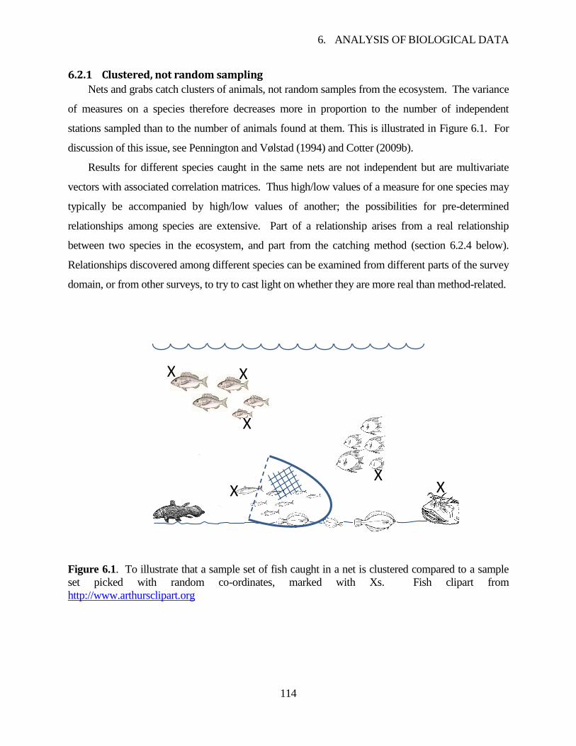
6. ANALYSIS OF BIOLOGICAL DATA

114

6.2.1 Clustered, not random sampling

Nets and grabs catch clusters of animals, not random samples from the ecosystem. The variance

of measures on a species therefore decreases more in proportion to the number of independent

stations sampled than to the number of animals found at them. This is illustrated in Figure 6.1. For

discussion of this issue, see Pennington and Vølstad (1994) and Cotter (2009b).

Results for different species caught in the same nets are not independent but are multivariate

vectors with associated correlation matrices. Thus high/low values of a measure for one species may

typically be accompanied by high/low values of another; the possibilities for pre-determined

relationships among species are extensive. Part of a relationship arises from a real relationship

between two species in the ecosystem, and part from the catching method (section 6.2.4 below).

Relationships discovered among different species can be examined from different parts of the survey

domain, or from other surveys, to try to cast light on whether they are more real than method-related.

Figure 6.1. To illustrate that a sample set of fish caught in a net is clustered compared to a sample

set picked with random co-ordinates, marked with Xs. Fish clipart from

http://www.arthursclipart.org

XX

X X

X

X

6. ANALYSIS OF BIOLOGICAL DATA

115

6.2.2 Non-stationary variation

Spatial and temporal variation of biological, sedimentary, and hydrological variables is typically

highly irregular in the sea with occasional extreme values. Consequently, assumptions of stationarity

underlying many parametric statistical methods are unsafe, e.g. „the mean and variance are constant‟.

Transformations of the data may give a good fit on one occasion but not another. Regional

estimation of indicators with confidence limits (CLs) based on the central limit theorem, as discussed

in section 3.4, does not depend on stationarity unless estimated values are later considered to apply

outside the survey domain, a risky assumption.

6.2.3 Zero abundances

Ecological measures cannot be made at all stations if the right animals are not found there.

Certain spatial indicators are not affected by zero values (Woillez et al., 2009) and geographic

distributions inferred from zero values can, by themselves, indicate declining fish stocks or climatic

effects for example. The effects of zeros can be avoided by reporting indicator values „given that the

species was caught‟ along with the stations of capture, or as „means-over-fish‟ which are estimates

weighted by the numbers of fish caught (Cotter, 2009b). Zeros interfere with logarithmic

transformation of real-valued measures intended to improve the validity of Gaussian (normal)

approximations to the statistical distribution. An arbitrary constant can be added to zero values but

analyses should be checked to see whether the Gaussian approximation is seriously affected by

different choices of constant. A well-known, model-based approach to survey zeros is given by

Pennington (1983). The treatment of zeros is often important and should be stated.

6.2.4 Covariances of signals and sampling errors

Variables measured by sampling on an EMS display variability for oceanographic or ecological

reasons, as well as variability deriving from the chosen methods of sampling, measurement, and

navigation. These are generally referred to as „signal‟ and „sampling errors‟ respectively. Covariance

or correlation (= standardized covariance) occurs when variation in one variable tends to occur in

association with variation in other. As a result, there is less information available from the two

variables than if they were independent or, in other words, given results for one variable, those for

the other can be predicted with precision depending on the degree of covariance.

Signal covariance arises

6. ANALYSIS OF BIOLOGICAL DATA

116

Between quantitative or biological measures from different species because of shared influences

of the ecosystem such as habitat, behaviour, feeding, climate, season, migrations, etc.

Between different measures from one species because individuals share influences of genetic,

physiological, and environmental factors.

Between physical and chemical measures because of the heterogeneity of water and sediments;

the closer the sampling points of two measures, the stronger the covariance tends to be.

Between biological measures and physical and chemical measures.

Signal covariance is one way of measuring the true relationships among ecosystem variables.

Ecosystem modellers estimate the relationships as mathematical functions.

Sampling covariance arises between different biological measures made on individuals taken

from

The same catch sample because of the manner of sampling the catch.

The same catch because of its specific location and timing.

The same catching device because of its specific selectivity properties and manner of

deployment.

The same cruise or survey repetition because of weather, crew, and any other influences on it.

Sampling covariance between physico-chemical measures arises from

Sampling units collected at the same incorrect locations and times.

Any analytical problems shared by the two measures.

Sampling covariance can distort the image of a signal provided by an EMS because sampling errors

are linked to variation of the sampling errors for the other measure. Sampling covariance can also

mislead by suggesting relationships between pairs of signals when the actual relationship is between

the sampling errors. This problem can beguile into over-interpretation of EMSs and over-determined

ecosystem models.

Covariance can also arise between signal and sampling error. An example would be when a

large catch prompts use of a faulty catch-sampling procedure that consistently under- or over-

estimates the quantity in the catch. Covariance of this type would cause exaggeration or damping of

signals.

6. ANALYSIS OF BIOLOGICAL DATA

117

6.2.5 Covariances between stations

Measures made at one station depend on ( = covary with) measures made at another when

Animals from adjacent stations are pooled to increase sample sizes. Some age-length keys are

compiled like this, causing numbers-at-age by station to become dependent and without

necessarily benefitting precision (Cotter and Pilling, 2007).

When stations are arrayed in a fixed-interval grid; positive serial correlation of results along the

lines is likely to be found.

When stations are randomly located in a regular lattice of strata (section 3.6); positive serial

correlation would usually be less than for a fixed grid because of the randomly varying distances

between stations.

When sampling methods differ regionally for operational reasons or due to inadequate training of

staff.

Independence of the results at each station means that each is providing information about the

ecosystem not estimable from other stations. It is important for finding the correct degrees of

freedom ( = number of stations – number of fitted parameters) for estimating regional variances and

covariances, for statistical tests relating to regional parameters, and for fitting models such as

contours which require independent data points.

6.3 Quantitative methods for analysis of EMS results

A small selection of quantitative methods is presented below.

6.3.1 Presence-absence data

Binary presence-absence and occupancies (section 5.1.1) are useful for monitoring species

whose abundance can only be measured with high sampling error, for example because

catchability is low

catching effort is poorly measured

shoaling behaviour or clumped distributions occur

the species is rare.

The idea is that the more abundant a species is within an ecosystem, the more stations it is likely to

be found at, given that it is moderately rare.

To see why occupancies are useful for poorly caught species, suppose that a species is found at

o out of n stations fished. Then, from the binomial distribution, the large-sample variance of the

6. ANALYSIS OF BIOLOGICAL DATA

118

occupancy, p o n , is var 1p pq n . It reduces to zero as the „true‟ p decreases to

zero. By contrast, the CV of the total abundance, a , of the species over all stations tends to infinity

as 0p (Cochran, 1977). p is therefore a much better measure than a for rare species.

Occupancies can be estimated for each survey or stratum domain and plotted over time. A practical

example showing their mostly low noise and responsiveness is in

6. ANALYSIS OF BIOLOGICAL DATA

119

Figure 5.2. The smoothed curves were derived from Bayesian ideas described in Box 5.1.

6.3.2 Ordered categorical data

Ecological measures in quantitative categories (e.g. „low‟, „medium‟, „high‟; or „1 – 9‟, ‟10 –

99‟, „100 – 999‟, etc.) have more quantitative information than presence-absence but less than real-

valued measures. These ordered categorical measures can be useful when real-valued measures are

thought to suffer from substantial, possibly irregularly distributed sampling errors, e.g. because of

bouncing trawls or variable corer volumes. Analysis and modelling of categorical measures is

discussed in a general text by Agresti (1996).

6.3.3 Ranked data

The simplest way of dealing with real-valued ecological measures is with nonparametric

statistics. They can be informative without reliance on strong assumptions, so they are most useful

when variability is high and the data are not clearly distributed according to a standard distribution

such as the Gaussian or lognormal distributions. The following notes are summarized from Cotter

(2009a) where more references can be found. A sample set of real measures is first put into

numerical order and ranks (1, 2, 3, . . . , N) are assigned.

The ordered measures can be summarized regionally using quantiles, usually the sample median,

conventionally the middle value for odd n or the average of the two middle values for even n .

Confidence limits are found using the binomial distribution. They get smaller as sample size

increases, as for the Central Limit Theorem applied to the mean. The median is slightly smaller than

the mean for skewed distributions such as the lognormal. It is less affected than the mean by

occasional large values in samples and may therefore have tighter, binomial confidence limits than

the mean has, based on the Central Limit Theorem. Quantiles can be interpreted in terms of areas or

time periods. For example, an ecosystem survey domain can be split into two equal areas where

measures are or > , respectively, the median value estimated from a cruise.

The median provides simple tests of trend in a time series with no assumptions about models,

transformations, residuals, etc.. In one test, consecutive measures are differenced, e.g. at lag 1:

2 1X X , 3 2X X , etc.. Then the median of the differences is zero when there is no trend,

and a significance test is provided by binomial confidence limits. A related median test is available

for before-after studies, and for comparisons of one stratum with another.

6. ANALYSIS OF BIOLOGICAL DATA

120

Greater detail on trends are obtainable with statistical methods that make full use of data

orderings. Kendall‟s tau and Spearman‟s rank correlation method test correlations between a

measure and the times of measurement. Jonckheere‟s method accommodates multiple observations

at each time. The aligned-rank test and the Dietz-Killeen test are for multivariate indicators. This

and other nonparametric tests find the probable direction of trends, up or down. Cochran‟s Q tests

whether all indicators are responding similarly over time, and the Runs test responds to serial

correlation around a quantile or trend.

6.3.4 Real-valued measures

Real-valued measures, eg. „length 21.3 cm‟, are typically analysed with parametric statistical

methods. Transformations, such as taking logarithms, may be necessary to encourage conformity

with standard statistical models such as the Gaussian distribution, or to improve the approximation to

Gaussian provided by the Central Limit Theorem. All the same, regional medians may prove more

stable and interpretable than regional means of transformed measures.

One of the main advantages of real-valued data is the opening up of modelling possibilities for

understanding and utilizing the results of ecosystem surveys. Contouring of indicator values over

stations is a general way of modelling. It can be carried out with various algorithms, e.g. Kriging,

using Geographic Information System software (GIS). Different patterns of contours can be

obtained with different algorithms, so residuals should be checked. References to specialized types of

model are given in section 0. Multispecies modelling in a fisheries context is reviewed by Pinnegar et

al. (2008). An ambitious, comprehensive, whole-ecosystem model, including socio-economic

submodels, is called Atlantis. It has been applied to many fished marine ecosystems globally (Fulton

et al., 2011).

Fulton et al. (2011) advise on the benefits and constraints of ecosystem modelling. From a

statistical viewpoint, the appeal of new predictions and insights must be balanced against the danger

of building model structure more elaborately than can be supported by available data and knowledge.

This is called over-determination or over-parameterization. It causes the model to become unstable

when one or more inputs are changed slightly; the model may also over-emphasize the effects of

trivial processes. Models can also be over-aggregated spatially, leading to excessively simplistic

conclusions. Fulton et al. (2011), citing Box (1979), state that „the art of modelling is to represent a

system in the simplest form consistent with realistically capturing its essential dynamics and

behaviour‟.

6. ANALYSIS OF BIOLOGICAL DATA

121

An important statistical aspect of monitoring indicators concerns whether they comply or not

with limits or reference values. This is part of the large subject of Statistical Quality Control (SQC)

(Montgomery, 2009). Marine ecosystem work appears to pose more challenges than the industrial

processes for which SQC methods were developed because variances and covariances of indicators

can be much more extreme, and time series tend to be short. The CUSUM method is particularly

suited for real-valued ecological indicators; see Mesnil and Petitgas (2009) for applications to

ecological indicators measured from trawl surveys. Making sense of many indicators moving in

different directions is a further challenge. Petitgas (2009) discusses a simple approach to multivariate

CUSUM charts. Numerous papers discuss applications of multivariate techniques more generally to

marine ecological data. Though good for research, they may not be so effective for formally

monitoring performance of ecosystem indicators because strong assumptions about statistical

distributions and large sample sizes may not be tenable.

6.3.5 Analysis of habitat indicators

Many benthic habitats are vulnerable to fishing gear on account of their fragile physical

structure. They may consist of soft mudbanks, reefs, or regions populated with attached epibenthic

fauna. Structure of benthic habitats can be monitored using acoustic and video techniques (Kenny et

al., 2003) supported by epibenthic or infaunal sampling. The critical questions are

Do the data collected signal a derioration in the habitat, no change, or an improvement?

If a deterioration, is it linked with fishing or any other manageable factors?

A suggested way to deal with the first question is to break the sampling points or tracks into

small quadrats and make an assessment in each using a cut-off value. For example, „structured

habitat present in < 30% of a 10 x 10m quadrat = poor‟. Quadrats should be located randomly so far

as possible or, if points fall along a linear track, a lattice of sampling strata could be overlayed and a

small number of points chosen randomly as sampling units from each square stratum. The lattice

design was discussed in section 3.6. A binary categorization of quadrats into „poor‟ or „good‟ habitat

could be assessed statistically over time as suggested above for occupancies by species. See section

5.1.1. Triple or higher categorization would require multinomial methods (Agresti, 1996).

The second question above might be dealt with by collecting commercial fishing-effort data by

large scale quadrats, eg. longitude-latitude rectangles, possibly using data from vessel monitoring

systems (VMS) (Eastwood et al., 2008) . Comparisons between trawling effort and benthic

6. ANALYSIS OF BIOLOGICAL DATA

122

communities in the same localities have been achieved by Rijnsdorp et al. (1998) and Zühlke et al.

(2001). Annual assessments of fishing effects might be made by testing change-of-indicator with

change-of-fishing-effort as pairs in each surveyed rectangle using a nonparametric test of

independence such as Kendall‟s tau or Spearman‟s rank correlation (Hollander and Wolfe, 1973).

6.3.6 Community indicators

Ecosystems consist of communities of species having mutually supportive functional roles.

Several community indicators have already been mentioned and it seems that there are few that make

special demands for the time of an RV ecosystem survey because the indicators can be estimated

from data already collected. Community size-based indicators like the proportion of large fish, the

proportionate size, and size spectra were put forward in the discussion of size-based indicators. A

community having a big proportion of large individuals will have the foodweb controlled by top

predators, will support secure reproduction of many species and, more practically, will give

protection to commercial fisheries against recruitment failures. Multi-species CPUE series may also

be valuable as community indicators providing that they are amenable to interpretation. Subsetting

into different functional groups would be beneficial for this, as discussed in section 0. Wide-scale

plankton monitoring may also cast light on community responses (Longhurst et al., 1995, Beaugrand,

2005). Other potentially informative community indicators are k-dominance curves (Lambshead et

al., 1983) which indicate whether one or two species are dominating a community, and ABC curves

(Warwick, 1986) which indicate whether the dominant individuals are large- or small-bodied.

Community indicators in second place for reasons discussed in section 5.1.1 are species richness,

species diversity, and the marine trophic index.

6.4 Conclusions

Several theoretical and practical constraints should be considered when analysing EMS data.

Many statistical and modelling methods are available for ecosystem measures of different types

according to precision, eg. presence-absence, ordered categorical, ranked, and real-valued measures.

Nonparametric statistical methods can be informative without making major assumptions about the

data. Modelling methods open up more structural possibilities but make stronger assumptions and

are dependent on the analyst identifying the model that represents the system in its simplest yet most

realistic form.

6. ANALYSIS OF BIOLOGICAL DATA

123

Monitoring changes in the structure of habitats can be carried out by classifying habitat quality

according to an arbitrary, but objective scale in randomized quadrats, or at random points in a lattice

of quadrats; the proportion of quadrats showing damage provides an indicator of habitat change.

When local-scale fishing effort is known, changes in habitat quality may be related to changes of

fishing effort in each quadrat using a nonparametric correlation method.

Community indicators can mostly be calculated from abundance, size, and weight data collected

by an ecosystem survey. Subsetting into different functional groups would assist interpretation of

community indicators. The proportion of large fish, the proportionate size, size spectra, multi-species

CPUE series, k-dominance and ABC curves, may all be valuable for indicating the health of marine

communities using RV surveys. Useful wide-scale supplementary information may be available

from satellite monitoring and continuous plankton recorder tows.

7. APPLYING SURVEY RESULTS FOR EAF

124

7 APPLYING EMS RESULTS FOR AN EAF MANAGEMENT

This section consists of notes on current issues for EAF fisheries management. Sometimes the

EAF will represent a development of single-species management procedures, as widely carried out

around the world. Resistance to new management policies suggested by the results of an EMS may

ensue because of the perceived security and practical advantages of the previous single-species

management system including, particularly, routine implementation and well understood input data.

These two advantages could beneficially be carried over so far as possible when seeking to apply

results of an EMS for the purposes of an EAF.

An EMS involves many species, indicators, and oceanographic measures. A significant risk

from this diversity is that management advice derived from an EMS lacks the structure and

dependability of single-species advice. There can also be issues of timing, quality control, and

understanding with new forms of advice (Apostolaki et al., 2008). The following features of an EMS

are suggested to help win acceptance:

(1) The EMS should follow an annual routine, ie. it is primarily for monitoring, not for research

unless special scientific work is requested and separately funded.

(2) The monitoring tasks, indicators, and performance measures should, if administratively possible,

be agreed by all influential parties in advance of EMS surveys, taking into account national and

international commitments to conservation, as well as RV resources and expense.

(3) The EMS should, so far as possible, supply the same body of results in the same format every

year, mostly as time series or changing maps. Dependability, consistent presentations, careful

descriptions of methods, and estimated levels of precision are all important for acceptability.

(4) Policy inferences should preferably be evident merely from graphic presentations of results with

standardized statistical techniques used in a supporting role. Dependence on strong technical

assumptions, ad hoc adjustments, and black box models could rapidly become obscure and

distrusted when there are many species and indicators to deal with at an EAF committee.

(5) Any procedures for modifying input or output controls on fisheries based on EMS results from

(4) should be agreed in advance, though they might be re-negotiated for future years to reflect

improved understanding of the ecosystem. This links back to (2) and should help to prevent

nasty surprises at EAF committee meetings. The agreed procedures will probably involve social

and economic time series as well as those from an EMS, as is consistent with the EAF.

7. APPLYING SURVEY RESULTS FOR EAF

125

Concerning (5), two ways to convert EMS monitoring results into decisions about fishery

controls are the reference point system, and ecological risk assessment for fisheries. In both cases, an

EAF committee, starting from status quo fishing, would probably wish to turn its attention first to the

most pressing issues gauged either by the reference points or the perceived risks. The following

notes about the two systems are meant to be impartial.

Reference points can be set as point values which should preferably not be crossed, upwards or

downwards as appropriate, by critical EMS time series. There may be two types, one a target, the

other a limit (Caddy and Mahon, 1995). Either type will probably need subjective decisions about

the values to use, eg. based on earlier periods of fishing history when the ecosystem was deemed

healthy and productive. Many reference points may be needed to protect all the vulnerable

components of an ecosystem. This implies that the ecosystem is tied down like a tent with pegs and

stays when, in reality, it is naturally highly variable. A problem that has perhaps not received enough

consideration is that testing compliance with reference points requires statistical quality control

(Montgomery, 2009), as already mentioned (section 6.3.4). High precision of the tests should not be

expected because of typically high variances and short time series for EMS indicators, so there are

high risks of making poor decisions. Somewhat less demanding for EAF than reference points are

reference directions of time series, ie. a reversal of trend from bad to good. However, statistical

confirmation of a reversal of trend takes a long time (Jennings and Dulvy, 2005) so supporting

reference points may be necessary as well. No actual values for reference points are suggested in this

report. It is envisaged that EAF committees managing fisheries and RV surveys will wish to set their

own reference points or directions, taking into account local circumstances and needs.

The second potential management framework for an EAF, ecological risk assessment for the

effects of fishing (ERAEF), was developed in Australia in response to early legislation calling for

protection of ecosystems there (Hobday et al., 2007, Astles, 2008). The general idea is that all the

components of an ecosystem, and all potentially harmful aspects of commercial fishing (and other

influences if required), are systematically considered to find the most important and damaging

effects, given agreed and detailed ecosystem and socio-economic objectives for managing the

fishery. This is analagous to dealing first with the points „where the shoe pinches‟. A preliminary

stage is a risk-screening process, called „Scale, intensity, and consequence analysis‟ (SICA), in which

individual units of all ecosystem components are briefly considered as being at low, medium, or high

risk from a comprehensive list of all the foreseen effects of fishing, given the expected scale and

7. APPLYING SURVEY RESULTS FOR EAF

126

intensity of fishing. The risks judged to be highest are passed on to „Productivity, susceptibility

analysis‟ (PSA) in which species are assessed for their „productivity‟ – meaning ability to recover

from fishing – based on life-history characteristics, and their susceptibility to fishing based on

availability to the gear, the likelihood of encounters, size selectivity, and post-capture mortality rates.

The highest risks from PSA may be passed on for more intensive study or modelling. A short review

and summary of ERAEF is given by Cotter and Lart (2011). General problems with ERAEF are that

it is only semi-quantitative, it depends on discovering all of the most pressing risks, and it does not

take into account actual fishing effort or catches. An EMS feeds into ERAEF by supplying updated

values of critical indicators so that performance relative to operational objectives and perceived risks

can be assessed.

8. CHECKLIST FOR AN ECOSYSTEM MONITORING SURVEY

127

8 CHECKLIST FOR AN RV ECOSYSTEM SURVEY

The list below summarizes and suggests an ordering of tasks for planning an RV ecosystem survey.

1. Prepare a background report on oceanography, fauna and flora, commercial fisheries, and any

other influences (section 2.2).

2. Fill a species database (Table 3.1) for the ecosystem.

3. Advise the EAF committee on definition of the ecosystem to be managed, the goals of

management, and on setting the general objectives (GOs) for ecosystem components,

indicators and performance measures (section 2.1).

4. Develop operational objectives (OOs) and associated indicators for the priority units (species,

or parts) of ecosystem components from the GOs decided at (3).

5. Set priorities for all underwater components to be surveyed (section 2.3) taking into account

goals, GOs, and OOs flowing from the EAF management committee .

6. Set priorities for all surface-dwelling components, including seabirds, marine mammals, and

perhaps other components to be watched from the EMS (sections 2.3.12, 2.3.13, 2.3.3) .

7. Assess RV options taking into account available fishing and sampling techniques, deck and

cabin space for working, the number of RVs required, safety and accommodation (section

2.4).

8. Choose and standardize fishing and other ecosystem sampling devices to be deployed

(section 2.5). Document all associated procedures in a protocol for each device.

9. Choose the survey domain taking into account catching and sampling techniques to be used

in different localities, species distributions, catchabilities on the survey, and vulnerabilities to

commercial fishing, so far as possible (section 3.1). Document in the survey protocol the

geography and timing of the survey domain in relation to the ecosystem agreed at (3),

recording reasons for choices made.

10. Choose the statistical survey design (sections 3.4 to 3.6), documenting reasons for the choices

in the survey protocol.

11. Choose indicators and performance measures to be applied to each ecosystem component

being surveyed; standardize the measures needed and the calculations to be made. (section

5). Document in catch or other sampling protocols associated with each deployed sampling

device.

8. CHECKLIST FOR AN ECOSYSTEM MONITORING SURVEY

128

12. Initiate discussions/negotiations at the EAF management committee on the interpretations

and implications of indicator movements as slopes, relative to reference values, or as

changing risks. (Section 7). Decide how indicators and performance measures will be

archived, processed and published. Document in an EMS analysis protocol.

13. Finalize and agree the protocols needed to standardize the survey design, fishing and other

sampling, catch processing, data checking and archiving, lists of species to be identified (if

closed lists will be used), how to deal with confusable or unidentifiable species, etc. (Section

4).

14. Train EMOs in catch processing and taxonomic skills. Train specialized EMOs for watching,

acoustic work, etc. Familiarize with relevant protocols. Test and certify their competence to

high standards.

9. REFERENCES

129

9 REFERENCES

Agresti, A. (1996) An introduction to categorical data analysis., Vol., John Wiley & Sons, Inc.,

New York.

Andersen, K.H., Pedersen, M. (2010) Damped trophic cascades driven by fishing in model marine

ecosystems. Proceedings of the Royal Society - Biological Sciences (Series B) 277, 795-802.

Anonymous (1998) Report of the study group on the evaluation of the quarterly IBTS surveys. ICES

CM International Council for the Exploration of the Sea, Copenhagen, No. ICES CM

1998/D:4.

Anonymous (2004) Report of the workshop on survey design and data analysis (WKSAD).

International Council for the Exploration of the Sea, Copehagen, No. ICES CM 2004/B:07,

Ref. D.G., 261pp. www.ices.dk/reports/FTC/2004/WKSAD04.pdf

Anonymous (2005) Report of the study group on survey trawl standardisation (SGSTS). ICES

Fisheries Technology Committee International Council for the Exploration of the Sea,

Copenhagen, No. ICES CM 2005/B:02. http://www.ices.dk/reports/FTC/2005/SGSTS05.pdf

Anonymous (2006) Report of the study group on survey trawl standardisation (SGSTS).

International Council for the Exploration of the Sea, No. ICES CM 2006/FTC:05, 67 pp.

http://www.ices.dk/products/cmdocs/2006/ftc/sgsts06.pdf

Anonymous (2007a) Development of EcoQO on changes in the proportion of large fish and

evaluation of size-based indicators. International Council for the Exploration of the Sea, No.

ICES ACE Report 2007.

Anonymous (2007b) Report of the working group on fish ecology (WGFE). International Council

for the Exploration of the Sea, Nantes, France, No. ICES CM 2007/LRC:03.

Anonymous (2009) Manual for the International Bottom Trawl Surveys. Revision VII. (Draft).

International Council for the Exploration of the Sea, Copenhagen.

http://www.ices.dk/datacentre/datras/NSIBTSmanualRevVIIdraft.pdf

Anonymous (2010) Manual for the international bottom trawl surveys in the western and southern

areas. Revision III. International Council for the Exploration of the Sea.

datras.ices.dk/Documents/Manuals/Addendum_2_Manual_IBTS_Western_and_Southern_A

reas_Revision_III.pdf - 2010-05-31

Anonymous (2011) Report of the expert workshop on the development and use of indicators for an

ecosystem approach to fisheries. FAO EAF-Nansen Project Food and Agriculture

Organization of the United Nations, Rome, No. FAO EAF-Nansen Project No. 7.

Apostolaki, P., Pilling, G.M., Armstrong, M.J., Metcalfe, J.D., Forster, R. (2008) Accumulation of

new knowledge and advances in fishery management: two complementary processes? In:

Advances in fisheries science 50 years on from Beverton and Holt. (Eds. A.I.L. Payne, J.

Cotter, T. Potter), Blackwell Publishing, pp. 229-254.

Armstrong, M.J., Payne, A.I.L., Cotter, A.J.R. (2008) Contributions of the fishing industry to

research through partnerships. In: Advances in fisheries science 50 years on from Beverton

and Holt. (Eds. A.I.L. Payne, A.J.R. Cotter, T. Potter), Blackwell Publishing, Oxford, UK.,

pp. 63-84.

Astles, K.L. (2008) A systematic approach to estimating ecological risks in marine fisheries. CABI

Reviews: Perspectives in Agriculture, Veterinary Science, Nutrition and Natural Resources 3,

16pp.

9. REFERENCES

130

Bache, A.J. (2002) Turtles, tuna and treaties: strengthening the links between international fisheries

management and marine species conservation. Journal of International Wildlife Law and

Policy 5, 49-64.

Bakun, A. (2006) Wasp-waist populations and marine ecosystem dynamics:navigating the “predator

pit” topographies. Progress in Oceanography 68.

Barnes, P.W., Thomas, J.P. (2005) Benthic habitats and the effects of fishing. Vol. Symposium 41.

American Fisheries Society, Bethesda, Md., p. 890pp.

Barnes, S.M., Maxwell, D., Reuman, D.C., Jennings, S. (2010) Global patterns in predator-prey size

relationships reveal size dependency of trophic transfer efficiency. Ecology 91, 222-232.

Bastian, T., Haberlin, D., Purcell, J.E., et al. (2011) Large-scale sampling reveals the spatio-temporal

distributions of the jellyfish Aurelia aurita and Cyanea capillata in the Irish Sea. Marine

Biology Online.

Batten, S.D., Clark, R., Flinkman, J., et al. (2003) CPR sampling: the technical background,

materials and methods, consistency and comparability. Progress in Oceanography 58, 193-

215.

Beaugrand, G. (2005) Monitoring pelagic ecosystems using plankton indicators. ICES Journal of

Marine Science 62, 333-338.

Begon, M., Harper, J.L., Townsend, C.R. (1996) Ecology; individuals, populations and communities,

3rd. edn Vol., Blackwell Science, Oxford, UK.

Benaka, L.R. (1999) Fish habitat: essential fish habitat and rehabilitation. Vol. Symposium 22.

American Fisheries Society, Hartford, CT.

Bianchi, G., Gislason, H., Graham, K., et al. (2000) Impact of fishing on size composition and

diversity of demersal fish communities. ICES Journal of Marine Science 57, 558-571.

Bivand, R.S., Pebesma, E.J., Gómez-Rubio, V. (2008) Applied spatial data analysis with R., (Use R!

Vol., Springer.

Bjarnason, B.A., Carlesi, M. (1992) Handlining and squid jigging. FAO Training Series no. 23.

Boyd, I.L., Bowen, W.D., Iverson, S.J. (2010) Marine mammal ecology and conservation: a

handbook of techniques., Oxford University Press.

Boyle, P., Rodhouse, P. (2005) Cephalopods: ecology and fisheries., Vol., Blackwell Science.

Branch, T.A., Watson, R., Fulton, E.A., et al. (2010) The trophic fingerprint of marine fisheries.

Nature 468, 431-435.

Brandt, A. (2006) Benthic protocols. Census of Antarctic Marine Life (CAML), 6pp.

http://www.caml.aq/benthos/documents/Benthos-Sampling.pdf

Breitburg, D.L., Riedel, G.F. (2005) Multiple stressors in marine systems. In: Marine Conservation

Biology; the science of maintaining the sea's biodiversity. (Eds. E.A. Norse, L.B. Crowder),

Island Press, Washington, pp. pp 167-182.

Brenke, N. (2005) An epibenthic sledge for operations on marine soft bottom and bedrock. Marine

Technology Society Journal 39, 10-21.

Buckland, S.T., Andersen, D.R., Burnham, K.P., Laake, J.L., Borchers, D.L., Thomas, L. (2004)

Advanced distance sampling., Oxford University Press, p. 430pp.

Buckland, S.T., Anderson, D.R., Burnham, K.P., Laake, J.L., Borchers, D.L., Thomas, L. (2001)

Introduction to distance sampling: estimating abundance of biological populations., Vol.,

Oxford University Press.

Caddy, J.F., Mahon, R. (1995) Reference points for fisheries management. FAO Fisheries Technical

Paper FAO, Rome, No. 347, 83 pp.

9. REFERENCES

131

Cadima, E.L., Caramelo, A.M., Afonso-Dias, M., Conte de Barros, P., Tandstad, M.O., De Leiva

Moreno, J.I. (2005) Sampling methods applied to fisheries science: a manual. Food and

Agriculture Organization of the United Nations, Rome, No. FAO Fisheries Technical Paper

434. http://www.fao.org/docrep/009/a0198e/A0198E00.htm#TOC

Callaway, R., Alsvåg, J., de Boois, I., et al. (2002a) Diversity and community structure of epibenthic

invertebrates and fish in the North Sea. ICES Journal of Marine Science 59, 1199-1214.

Callaway, R., Engelhard, G.H., Dann, J., Cotter, J., Rumohr, H. (2007) One century of North Sea

epibenthos and trawling: comparison between 1902-1912, 1982-1985 and 2000. Marine

Ecology Progress Series 346, 27-43.

Callaway, R., Jennings, S., Lancaster, J., Cotter, J. (2002b) Mesh-size matters in epibenthic surveys.

Journal of the Marine Biological Association of the United Kingdom 82, 1-8.

Campana, S.E. (2005) Otolith science entering the 21st century. Marine and Freshwater Research

56, 485-495.

Carrier, J.C., Musick, J.A., Heithaus, M.R. (2010) Sharks and their relatives II; biodiversity, adaptive

physiology, and conservation. Vol. 2. CRC Press.

Casini, M., Lövgren, J., Hjelm, J., Cardinale, M., Molinero, J.-C., Kornilovs, G. (2008) Multi-level

trophic cascades in a heavily exploited open marine ecosystem. Proceedings of the Royal

Society - Biological Sciences (Series B) 275, 1793-1801.

Charnov, E.L. (1993) Life history invariants., Vol., Oxford University Press, Oxford.

Checkley, D.M.J., Alheit, J., Oozeki, Y., Roy, C. (2009) Climate change and small pelagic fish.,

Cambridge University Press.

Chouinard, G.A., Parent, K., Robichaud-Leblanc, K., Daigle, D. (1999) Results of the sentinel

surveys for cod conducted in the southern Gulf of St. Lawrence in 1994-1998. Research

document Canadian Stock Assessment Secretariat, Fisheries and Oceans, Ottawa, No. 99/24,

1-56.

Christensen, V., Walters, C.J. (2004) Ecopath with Ecosim: methods, capabilities, and limitations.

Ecological Modelling 172, 109-139.

Clarke, E.D., Spear, L.B., McCracken, M.L., et al. (2003) Validating the use of generalized additive

models and at-sea surveys to estimate size and temporal trends of seabird populations.

Journal of Applied Ecology 40, 278-292.

Claudet, J. (2011) Marine protected areas: a multidisciplinary approach., Cambridge University

Press.

Cochran, W.G. (1977) Sampling techniques., Vol., J. Wiley & Sons, Inc., New York.

Conover, W.J. (1971) Practical nonparametric statistics., Vol., John Wiley & Sons, New York.

Cortès, E. (2008) Comparative life history and demography of pelagic sharks. In: Sharks of the open

ocean: biology, fisheries and conservation. (Eds. M.D. Camhi, E.K. Pikitch, E. Babcock),

Blackwell, Oxford, UK, pp. 309-322.

Cotter, A.J.R. (1985) Water quality surveys: a statistical method based on determinism, quantiles and

the binomial distribution. Water Research 19, 1179-1189.

Cotter, A.J.R. (1998) Method for estimating variability due to sampling of catches on a trawl survey.

Canadian Journal of Fisheries & Aquatic Sciences 55, 1607-1617.

Cotter, A.J.R. (2008) The "soundscape" of the sea, underwater navigation, and why we should be

listening more. In: Advances in fisheries science; 50 years on from Beverton and Holt. (Eds.

A.I.L. Payne, J. Cotter, T. Potter), Blackwell Publishing Ltd, Oxford, pp. 451-471.

9. REFERENCES

132

Cotter, A.J.R. (2009a) A selection of nonparametric statistical methods for assessing trends in trawl

survey indicators as part of an ecosystem approach to fisheries management (EAFM).

Aquatic Living Resources 22, 173-186.

Cotter, A.J.R. (2009b) Statistical estimation of mean values of fish stock indicators from trawl

surveys. Aquatic Living Resources 22, 127-134.

Cotter, A.J.R., Pilling, G.M. (2007) Landings, logbooks and observer surveys: improving the

protocols for sampling commercial fisheries. Fish and Fisheries 8, 123-152.

Cotter, A.J.R., Rogers, S., Ellis, J., et al. (2008) Marine Ecosystem Integrity: Development of a

Marine Trophic Index for UK waters and recommendations for further indicator

development. Cefas, Lowestoft, UK, No. Cefas contract report No. C3140.

Cotter, J., Lart, W. (2011) A guide for ecological risk assessment of the effects of commercial fishing

(ERAEF). Sea Fish Industry Authority, Grimsby, UK, 78pp.

http://sin.seafish.org/portal/site/sin/

Cotter, J., Mesnil, B., Witthames, P., Parker-Humphreys, M. (2009) Notes on nine biological

indicators estimable from trawl surveys with an illustrative assessment for North Sea cod.

Aquatic Living Resources 22, 135-154.

Course, G.P., Cotter, A.J.R., Jolliffe, R.O., Kay, B.J., Rolfe, M.S. (1999) Safe practices for sampling

commercial trawler catches at sea. Fisheries Research 41, 99-104.

Currie, D.R., Sorokin, S.J., Ward, T.M. (2008) Performance assessment of the benthic protection

zone of the Great Australian Bight marine park. South Australian Department for

Environment and Heritage,

Commonwealth Dept. of the Environment and Water Resources, No. Final report F2008/000647-1,

113pp.

Cury, P., Bakun, A., Crawford, R.J.M., et al. (2000) Small pelagics in upwelling systems: patterns of

interaction and structural changes in „„wasp-waist‟‟ ecosystems. ICES Journal of Marine

Science 57, 603-618.

Daan, N. (2001) The IBTS database: a plea for quality control. No. ICES CM 2001/T:3.

Daskalov, G.M. (2008) Overfishing affects more than fish populations: a case of trophic cascades

and regime shifts in the Black Sea. In: Advances in fisheries science 50 years on from

Beverton and Holt. (Eds. A.I.L. Payne, A.J.R. Cotter, T. Potter), Blackwell Publishing,

Oxford, UK., pp. 418-433.

Dulvy, N.K., Ellis, J.R., Goodwin, N.B., Grant, A., Reynolds, J.D., Jennings, S. (2004) Methods of

assessing extinction risk in marine fishes. Fish and Fisheries 5, 255-276.

Dulvy, N.K., Forrest, R.E. (2010) Life histories, population dynamics and extinction risks in

chondrichthyans. In: Biology of sharks and their relatives. (Eds. J.C. Carrier, J.A. Musick,

M.R. Heithaus), CRC Press, Washington, D.C., pp. pp. 635-675.

Dulvy, N.K., Jennings, S., Rogers, S.I., Maxwell, D.L. (2006) Threat and decline in fishes: an

indicator of marine biodiversity. Canadian Journal of Fisheries & Aquatic Sciences 63,

1267-1275.

Dunne, J.A., Williams, R.J. (2009) Cascading extinctions and community collapse in model food

webs. Philosophical Transactions of the Royal Society, B-Biological Sciences. 364, 1711-

1723.

Eastwood, P.D., Meaden, G.J., Nishida, T., Rogers, S.I. (2008) Understanding and managing marine

fisheries with the aid of a digital map. In: Advances in fisheries science 50 years on from

Beverton and Holt. (Eds. A.I.L. Payne, J. Cotter, T. Potter), Blackwell Publishing, pp. 85-

103.

9. REFERENCES

133

Eleftheriou, A. (2000) Marine benthos dynamics: environmental and fisheries impacts. In: ICES

Journal of Marine Science. Vol. 57(5). pp. 1299-1523.

Ellis, J.R., Clarke, M.W., Cortès, E., et al. (2008) Management of elasmobranch fisheries in the

North Atlantic. In: Advances in fisheries science 50 years on from Beverton and Holt. (Eds.

A.I.L. Payne, J. Cotter, T. Potter), Blackwell Publishing, pp. 184-228.

FAO (1995) Code of conduct for responsible fisheries. Food and Agriculture Organization of the

United Nations, Rome, 40 pp.

FAO (1999) Indicators for sustainable development of marine capture fisheries. FAO technical

guidelines for responsible fisheries 8, 68pp.

FAO (2003) Fisheries management: 2. the ecosystem approach to fisheries. FAO Technical

Guidelines for Responsible Fisheries. 4, 112pp.

FAO (2005) Putting into practice the ecosystem approach to fisheries. Food and Agriculture

Organization, Rome, No. ISBN 9789251053966, 82pp.

ftp://ftp.fao.org/docrep/fao/008/a0191e/a0191e00.pdf

FAO (2008) Fisheries management. 2. The ecosystem approach to fisheries. 2.1 Best practices in

ecosystem modelling for informing an ecosystem approach to fisheries. Fisheries Technical

Guidelines for Responsible Fisheries. Food and Agriculture Organization, Rome, No. No. 4,

Suppl. 2, Add. 1, 78pp. ftp://ftp.fao.org/docrep/fao/011/i0151e/i0151e00.pdf

Feller, W. (1968) An introduction to probability theory and its applications., 3rd. edn Vol., J. Wiley,

New York.

Fletcher, W.J., Chesson, J., Sainsbury, K., Hundloe, T.J., Fisher, M. (2005) A flexible and practical

framework for reporting on ecologically sustainable development for wild capture fisheries.

Fisheries Research 71, 175-183.

Fox, C.J., Aldridge, J.N. (2008) Simulating the marine environment and its use in fisheries research.

In: Advances in fisheries research 50 years on from Beverton and Holt. (Eds. A.I.L. Payne,

J. Cotter, T. Potter), Blackwell Publishing, pp. 399-417.

Fromentin, J.M., Royer, F., Marsac, F. (2005) Open environmental databases for open-sea fisheries

biologists. ICCAT Collected Volume of Science Papers 58, 1756-1760.

Fulton, E.A., Link, J.S., Kaplan, I.C., et al. (2011) Lessons in modelling and management of marine

ecosystems: the Atlantis experience. Fish and Fisheries 12, 171-188.

Galgani, F., Burgeot, T., Bocquene, G., Vincent, F., Leaute, J.P., Labastie, J. (1995) Distribution and

abundance of debris on the continental shelf of the Bay of Biscay and in Seine Bay. Marine

Pollution Bulletin 30, 58-62.

Galil, B.S., Golik, A., Turkay, M. (1995) Litter at the bottom of the sea: a sea bed survey in the

eastern Mediterranean. Marine Pollution Bulletin 30, 22-24.

Goss, C., Middleton, D., Rodhouse, P. (2001) Investigations of squid stocks using acoustic survey

methods. Fisheries Research 54, 111-121.

Gray, M. (2010a) Environmental data gathering for environmental assessments - basic seabed habitat

mapping using acoustic ground discrimation sonar and underwater video. Sea Fish Industry

Authority, Grimsby, UK., No. SR637, 32pp. www.seafish.org

Gray, M. (2010b) Seafish standard sampling operating procedure: basic video mapping seabed

habitat. Sea Fish Industry Authority, Grimsby, UK., No. SR639. www.seafish.org

Gubbay, S. (1995) Marine protected areas. Principles and techniques for management. In:

Conservation biology series. Chapman & Hall, London.

Hamlett, W.C. (1999) Sharks, skates and rays. The biology of elasmobranch fishes., John Hopkins

University Press, Baltimore.

9. REFERENCES

134

Haslob, H., Clemmesen, C., Schaber, M., et al. (2007) Invading Mnemiopsis leidyi as a potential

threat to Baltic fish. Marine Ecology Progress Series 349, 303-306.

Hays, G.C., Bastian, T., Doyle, T.K., et al. (2011) High activity and Levy searches: jellyfish can

search the water column like fish. Proceedings of the Royal Society - Biological Sciences

(Series B) Online.

Hays, G.C., Richardson, A.J., Robinson, C. (2006) Climate change and marine plankton. Trends in

Ecology and Evolution 20, 337-344.

Hempel, G., Sherman, K. (2003) Large marine ecosystems of the world: trends in exploitation,

protection, and research. In: Large Marine Ecosystems series. Vol. 12. Elsevier.

Hiddink, J.G., Hutton, T., Jennings, S., Kaiser, M.J. (2006a) Predicting the effects of area closures

and fishing effort restrictions on the production, biomass, and species richness of benthic

invertebrate communities. ICES J. Mar. Sci. 63, 822-830.

Hiddink, J.G., Jennings, S., Kaiser, M.J. (2006b) Indicators of the ecological impact of bottom-trawl

disturbance on seabed communities. Ecosystems 9, 1190.

Hobday, A.J., Smith, A., Webb, H., et al. (2007) Ecological risk assessment for the effects of fishing:

methodology. Australian Fisheries Management Authority, Canberra, No. Report R04/1072,

174 pp. www.afma.gov.au

Hoelzel, A.R. (2002) Marine mammal biology: an evolutionary approach., Blackwell Science.

Holden, M.J., Raitt, D.F.S. (1974) Manual of fisheries science part 2 - Methods of resource

investigation and their application. In: FAO Corporate Document Repository. Food and

Agriculture Organization of the United Nations, Rome.

Hollander, M., Wolfe, D.A. (1973) Nonparametric statistical methods., Vol., John Wiley & Sons,

New York.

Houghton, J.D.R., Doyle, T.K., Davenport, J., Hays, G.C. (2006) Developing a simple, rapid method

for identifying and monitoring jellyfish aggregations from the air. Marine Ecology Progress

Series 314, 159-170.

Hyrenbach, K.D., Henry, M.F., Morgan, K.H., Welch, D.W., Sydeman, W.J. (2007) Optimizing the

width of strip transects for seabird surveys from vessels of opportunity. Marine Ornithology

35, 29-38.

Jackson, J.E. (2003) A user's guide to principal components., Vol., J. Wiley, New York.

Jennings, S., Dulvy, N.K. (2005) Reference points and reference directions for size-based indicators

of community structure. ICES Journal of Marine Science 62, 397-404.

Jennings, S., Greenstreet, S.P.R., Hill, L., Piet, G.J., Pinnegar, J.K., Warr, K.J. (2002a) Long-term

trends in the trophic structure of the North Sea fish community: evidence from stable-isotope

analysis, size-spectra and community metrics. Marine Biology 141, 1085-1097.

Jennings, S., Lancaster, J., Woolmer, A., Cotter, J. (1999) Distribution, diversity and abundance of

epibenthic fauna in the North Sea. Journal of the Marine Biological Association of the United

Kingdom 79, 385-399.

Jennings, S., Warr, K.J., Mackinson, S. (2002b) Use of size-based production and stable isotope

analyses to predict trophic transfer efficiencies and predator-prey body mass ratios in food

webs. Marine Ecology Progress Series 240, 11-20.

Jensen, A.L. (1997) Origin of the relation between K and Linf and synthesis of relations among life

history parameters. Canadian Journal of Fisheries & Aquatic Sciences 54, 987-989.

Kaiser, M.J. (1998) Significance of bottom-fishing disturbance. Conservation Biology 12, 1230-

1235.

9. REFERENCES

135

Kenny, A.J., Cato, I., Desprez, M., Fader, G., Schu¨ttenhelm, R.T.E. (2003) An overview of seabed-

mapping technologies in the context of marine habitat classification. ICES Journal of Marine

Science 60, 411-418.

Kiorboe, T. (2008) A mechanistic approach to plankton ecology., Vol., Princeton University Press,

Princeton, NJ.

Kirby, R.R., Beaugrand, G. (2009) Trophic amplification of climate warming. Proceedings of the

Royal Society - Biological Sciences (Series B) 276, 4095-4103.

Kjesbu, O.S., Hunter, J.R., Witthames, P.R. (2003) Report of the working group on modern

approaches to assess maturity and fecundity of warm- and cold-water fish and squids.

Institute of Marine Research, Bergen, Norway, No. Fisken og havet, 12, 140 pp.

Lambshead, P.J.D., Platt, H., Shaw, K. (1983) The detection of differences among assemblages of

marine benthic species based on an assessment of dominance and diversity. Journal of

Natural History 17, 859-874.

Lewis, M. (2009) Sherman the epibenthic sled for rough terrain. CSIRO, Hobart, Tasmania, No.

Marine and Atmospheric Research Paper 029. http://www.cmar.csiro.au/e-

print/open/2009/lewism_a.pdf

Lindley, J.A., Gamble, J.C., Hunt, H.G. (1995) A change in the zooplankton of the central North Sea

(55o to 58o N): a possible consequence of changes in the benthos. Marine Ecology Progress

Series 119, 299-303.

Longhurst, A., Sathyendranath, S., Platt, T., Caverhill, C. (1995) An estimate of global primary

production in the ocean from satellite radiometer data. Journal of Plankton Research 17,

1245-1271.

Longhurst, A.R. (2007) Ecological geography of the sea., Vol., Academic Press.

Lutz, P.L., Musick, J.A. (1996) The biology of sea turtles., Vol., CRC Marine Science Series.

Lynam, C.P., Gibbons, M.J., Bjorn, E.A., et al. (2006) Jellyfish overtake fish in a heavily fished

ecosystem. Current Biology 16, R492-R493.

MacLennan, D.N., Simmonds, E.J. (2010) Fisheries acoustics., (Fish and Fisheries Series, Vol.,

Chapman & Hall.

Medwin, H., Clay, C.S. (1998) Fundamentals of acoustical oceanography., Vol., Academic Press,

Boston.

Mesnil, B., Petitgas, P. (2009) Detection of changes in time series of indicators using CUSUM

control charts. Aquatic Living Resources 22, 187-192.

Metcalfe, J.D., Righton, D.A., Hunter, E., Neville, S., Mills, D.K. (2008) New technologies for the

advancement of fisheries science. In: Advances in fisheries science 50 years on from

Beverton and Holt. (Eds. A.I.L. Payne, J. Cotter, T. Potter), Blackwell Publishing.

Milton, D.A. (2001) Assessing the susceptibility to fishing of rare trawl bycatch: sea snakes caught

by Australia's northern prawn fishery. Biological Conservation 101, 281-290.

Mitson, R.B., Knudsen, H.P. (2003) Causes and effects of underwater noise on fish abundance

estimation. Aquatic Living Resources 16, 255-263.

Montgomery, D.C. (2009) Statistical quality control: a modern introduction., 6th. edition edn Vol., J.

Wiley.

Ona, E., Godø, O.R., Handegard, N.O., Hjellvik, V., Patel, R., Pedersen, G. (2007) Silent research

vessels are not quiet. Journal of the Acoustical Society of America 121, EL145-EL150.

Onley, D., Scofield, P. (2007) Albatrosses, petrels and shearwaters of the world., Vol., Helm Field

Guides, London.

9. REFERENCES

136

Patten, M.A., Smith-Patten, B.D. (2011) Predictors of occupancy trend across spatial scale.

Conservation Biology.

Pauly, D. (1995) Anecdotes and the shifting baseline syndrome of fisheries. Trends in Ecology and

Evolution 10, 430.

Pauly, D., Watson, R. (2005) Background and interpretation of the „Marine Trophic Index‟ as a

measure of biodiversity. Philosophical Transactions of the Royal Society, B-Biological

Sciences. 360, 415-423.

Pennington, M. (1983) Efficient estimators of abundance, for fish and plankton surveys. Biometrics

39, 281-286.

Pennington, M., Vølstad, J.H. (1991) Optimum size of sampling unit for estimating the density of

marine populations. Biometrics 47, 717-723.

Pennington, M., Vølstad, J.H. (1994) Assessing the effect of intra-haul correlation and variable

density on estimates of population characteristics from marine surveys. Biometrics 50, 725-

732.

Petitgas, P. (2009) The CUSUM out-of-control table to monitor changes in fish stock status using

many indicators. Aquatic Living Resources 22, 201-206.

Petitgas, P., Poulard, J.C. (2009) A multivariate indicator to monitor changes in spatial patterns of

age-structured fish populations. Aquatic Living Resources 22, 165-172.

Pinnegar, J.K., Trenkel, V.M., Blanchard, J.L. (2008) 80 years of multispecies fisheries modelling:

significant advances and continuing challenges. In: Advances in fisheries science 50 years on

from Beverton and Holt. (Eds. A.I.L. Payne, J. Cotter, T. Potter), Blackwell Publishing, pp.

325-357.

Pope, J.G., Rice, J.C., Daan, N., Jennings, S., Gislason, H. (2006) Modelling an exploited marine fish

community with 15 parameters - results from a simple size-based model. ICES Journal of

Marine Science 63, 1029-1044.

Ranft, R.D. (1997) Bioacoustic libraries and recordings of aquatic animals. Marine and Freshwater

Behaviour and Physiology 29, 251-262.

Rees, H.L., Ellis, J.R., Hiscock, K., Boyd, S.E., Schratzberger, M. (2008) Benthic communities,

ecosystems and fisheries. In: Advances in fisheries science 50 years on from Beverton and

Holt. (Eds. A.I.L. Payne, A.J.R. Cotter, T. Potter), Blackwell Publishing, Oxford.

Reid, P.C., Battle, E.J.V., Batten, S.D., Brander, K.M. (2000) Impacts of fisheries on plankton

community structure. ICES Journal of Marine Science 57, 495-502.

Reiss, H., Degraer, S., Duineveld, G.C.A., et al. (2010) Spatial patterns of infauna, epifauna, and

demersal fish communities in the North Sea. ICES Journal of Marine Science 67, 278-293.

Richardson, A.J., Bakun, A., Hays, G.C., Gibbons, M.J. (2009) The jellyfish joyride: causes,

consequences and management responses to a more gelatinous future. Trends in Ecology and

Evolution 24, 312-322.

Rijnsdorp, A.D., Buys, A.M., Storbeck, F., Visser, E.G. (1998) Micro-scale distribution of beam

trawl effort in the southern North Sea between 1993 and 1996 in relation to the trawling

frequency of the sea bed and the impact on benthic organisms. ICES Journal of Marine

Science 55, 403-419.

Rilov, G., Crooks, J.A. (2009) Biological invasions in marine ecosystems: ecological, management,

and geographic perspectives., Springer-Verlag, Berlin.

Rochet, M.-J., Cornillon, P.A., Sabatier, R., Pontier, D. (2000) Comparative analysis of phylogenetic

and fishing effects in life history patterns of Teleost fishes. Oikos 91, 255-270.

9. REFERENCES

137

Schlacher, T.A., Wooldridge, T.H. (1996) How sieve mesh-size affects sample estimates of estuarine

benthic macrofauna. Journal of Experimental marine biology and ecology 201, 159-171.

Schmitt, S.A. (1969) Measuring uncertainty. An elementary introduction to Bayesian statistics.,

Vol., Addison-Wesley, Philippines.

Schratzberger, M., Gee, J.M., Rees, H.L., Boyd, S.E., Wall, C.M. (2000) The structure and

taxonomic composition of sublittoral meiofauna assemblages as an indicator of the status of

marine environments. Journal of the Marine Biological Association of the United Kingdom

80, 969-980.

Schreiber, E.A., Burger, J. (2001) Biology of marine birds., CRC marine biology.

Sherman, K., Duda, A.M. (1999) Large marine ecosystems: an emerging paradigm for fishery

sustainability. Fisheries 24, 15-26.

Shin, Y.-J., Cury, P.M. (2004) Using an individual-based model of fish assemblages to study the

response of size spectra to changes in fishing. Canadian Journal of Fisheries & Aquatic

Sciences 61, 414-431.

Shin, Y.-J., Rochet, M.-J., Jennings, S., Field, J.G., Gislason, H. (2005) Using size-based indicators

to evaluate the ecosystem effects of fishing. ICES Journal of Marine Science 62, 384-396.

Shirihai, H., Jarrett, B. (2006) Whales, dolphins and seals. A field guide to the marine mammals of

the world., Vol., A & C Black, London.

Simmonds, J.E., MacLennan, D.N. (2005) Fisheries Acoustics: Theory and Practice., Vol.,

Blackwell Science.

Smith, A.D.M., Brown, C.J., Bulman, C.M., et al. (2011) Impacts of Fishing Low–Trophic Level

Species on Marine Ecosystems. Sciencexpress, 5pp.

Spaulding, M.D., Fox, H.E., Allen, G.R., et al. (2007) Marine Ecoregions of the World: A

Bioregionalization of Coastal and Shelf Areas. Bioscience 57, 573-583.

Spotila, R. (2004) Sea turtles: a complete guide to their biology, behavior, and conservation., Vol.,

John Hopkins University Press and Oakwood Arts.

Stauffer, G. (2003) NOAA protocols for groundfish bottom trawl surveys of the nation's fishery

resources. NOAA Technical Memorandum U.S. Dep. Commerce, No. NMFS-F/SPO-65,

205 pp. http://spo.nmfs.noaa.gov/tm/

Stone, R. (2010) Chinese initiative amis to comprehend and combat a slimy foe. Science 330, 1464-

1465.

Stratoudakis, Y., Bernal, M., Ganias, K., Uriarte, A. (2006) The daily egg production method: recent

advances, current applications and future challenges. Fish and Fisheries 7, 35-57.

Suthers, I.M., Rissik, D. (2009) Plankton: a guide to their ecology and monitoring for water quality.,

CSIRO publishing, p. 272pp.

Tasker, M.L., Hope Jones, P., Dixon, T., Blake, B.F. (1984) Counting Seabirds at Sea from Ships: A

Review of Methods Employed and a Suggestion for a Standardized Approach. The Auk 101,

567-577.

Thomas, L., Burnham, K.P., Buckland, S.T. (2004) Temporal inferences from distance sampling

surveys. In: Advanced distance sampling. (Eds. S.T. Buckland, D.R. Andersen, K.P.

Burnham, J.L. Laake, D.L. Borchers, L. Thomas), Oxford University Press, pp. 71-107.

Thompson, S.K. (1992) Sampling, Vol., John Wiley & Sons, Inc., New York.

Tillin, H.M., Hiddink, J.G., Jennings, S., Kaiser, M.J. (2006) Chronic bottom trawling alters the

functional composition of benthic invertebrate communities on a sea-basin scale. Marine

Ecology Progress Series 318, 31-45.

9. REFERENCES

138

Trenkel, V.M., Cotter, A.J.R. (2009) Choosing survey time series for populations as part of an

ecosystem approach to fishery management. Aquatic Living Resources 22, 121-126.

Trippel, E.A. (1995) Age at maturity as a stress indicator in fisheries. Bioscience 45, 759-771.

Trippel, E.A. (2003) Reproductive potential of fish populations of the North Atlantic. In: Journal of

northwest Atlantic Fishery Science. Vol. 33. Northwest Atlantic Fisheries Organization,

Dartmouth, Nova Scotia, p. 214 pp.

Ward, P., Lawrence, E., others (2008) Large-scale experiment shows that nylon leaders reduce shark

bycatch and benefit pelagic longline fishers. Fisheries Research 90, 100-108.

Ward, T.M., Sorokin, S.J., Currie, D.R., Rogers, P.J., McLeay, L.J. (2006) Epifaunal assemblages of

the eastern Great Australian Bight: effectiveness of a benthic protection zone in representing

regional biodiversity. Continental Shelf Research 26, 25-40.

Ward, T.M., Sorokin, S.J., Rogers, P.J., McLeay, L.J., Turner, D.J. (2003) Benthic protection zone of

the Great Australian Bight marine park: 3. Pilot study for performance assessment (Volume

1). South Australian R & D Institute (Aquatic Sciences), West Beach, South Australia 5024,

No. Final report to National Parks and Wildlife, SA.

http://www.environment.gov.au/coasts/mpa/publications/pubs/gab-benthic-protection-

pilot.pdf

Warwick, R.M. (1986) A new method for detecting pollution effects on marine macrobenthic

communities. Marine Biology 92, 557-562.

Weinberg, K.L., Kotwicki, S. (2008) Factors influencing net width and sea floor contact of a survey

trawl. Fisheries Research 93, 265-279.

Willis, D.W., Murphy, B.R., Guy, C.S. (1993) Stock density indices: development, use, and

limitations. Reviews in Fisheries Science 1, 203-222.

Witthames, P.R., Marshall, C.T. (2008) The importance of reproductive dynamics in fish stock

assessments. In: Advances in fisheries science 50 years after Beverton and Holt. (Eds. A.I.L.

Payne, J. Cotter, T. Potter), Blackwell Publishing, pp. 306-324.

Woillez, M., Rivoirard, J., Petigas, P. (2009) Notes on survey-based spatial indicators for monitoring

fish populations. Aquatic Living Resources 22, 155-164.

Zuhlke, R., Alvsvag, J., De Boois, I., et al. (2001) Epibenthic diversity in the North Sea.

Senckenbergiana Maritima 31, 269-281.

Zuur, A.F., Pierce, G.J. (2004) Common trends in Northeast Atlantic squid time series. Journal of

Sea Research 52, 57-72.