L15_Arrays3

8/12/2019 L15_Arrays3

http://slidepdf.com/reader/full/l15arrays3 1/23

Nikolova 2012 1

LECTURE 15: LINEAR ARRAYS – PART III( N-element linear arrays with uniform spacing and non-uniform amplitude:

Binomial array; Dolph–Tschebyscheff array. Directivity and design. )

1. Advantages of linear array with nonuniform amplitude

The most often met BSAs, classified according to the type of their excitationamplitude, are:

a) the uniform BSA – relatively high directivity, but the side-lobe levels arehigh;

b) Dolph–Tschebyscheff (Chebyshev, Чебышёв ) BSA – for a given numberof elements maximum directivity is next after that of the uniform BSA;side-lobe levels are the lowest in comparison with the other two types of

arrays for a given directivity;c) binomial BSA – does not have good directivity but has very low side-lobe

levels (when / 2d , there are no side lobes at all).

2. Array factor (AF) of a linear array with nonuniform amplitudedistribution

Let us consider a linear array with an even number (2 M ) of elements,located symmetrically along the z -axis, with excitation, which is alsosymmetrical with respect to 0 z . For a broadside array ( 0) ,

1 3 2 1cos cos cos

2 2 21 2

1 3 2 1cos cos cos

2 2 21 2

...

... ,

M j kd j kd j kd e

M

M j kd j kd j kd

M

AF a e a e a e

a e a e a e

(15.1)

1

2 12 cos cos

2

M e

nn

n AF a kd

. (15.2)

If the linear array consists of an odd number (2 M +1) of elements, locatedsymmetrically along the z -axis, the array factor is

cos 2 cos cos1 2 3 1

cos 2 cos cos2 3 1

2 ...

... ,

o jkd j kd jMkd M

jkd j kd jMkd M

AF a a e a e a e

a e a e a e

(15.3)

1

1

2 cos 1 cos M

on

n

AF a n kd . (15.4)

8/12/2019 L15_Arrays3


Nikolova 2012 2

EVEN - AND ODD - NUMBER ARRAYS

Fig. 6.17, p. 291, Balanis

8/12/2019 L15_Arrays3


Nikolova 2012 3

The normalized AF derived from (15.2) and (15.4) can be written in the form

1

cos (2 1) , M

en

n

AF a n u for 2 N M , (15.5)

1

1cos 2( 1) ,

M

o nn

F a n u for 2 1 N M , (15.6)

where1

cos cos2

d u kd

.

Examples of AFs of arrays of nonuniform amplitude distribution

a) uniform amplitude distribution ( N = 5, / 2d , max. at 0 90 °)

p. 148-149, Stutzman

8/12/2019 L15_Arrays3


Nikolova 2012 4

b) triangular (1:2:3:2:1) amplitude distribution ( N = 5, / 2d , max. at0 90 °)


8/12/2019 L15_Arrays3


Nikolova 2012 5

c) binomial (1:4:6:4:1) amplitude distribution ( N = 5, / 2d , max. at0 90 °)


8/12/2019 L15_Arrays3


Nikolova 2012 6

d) Dolph-Tschebyschev (1:1.61:1.94:1.61:1) amplitude distribution ( N = 5,/ 2d , max. at 0 90 °)


8/12/2019 L15_Arrays3


Nikolova 2012 7

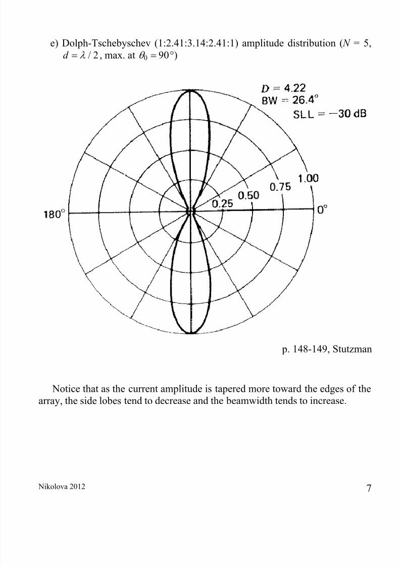
e) Dolph-Tschebyschev (1:2.41:3.14:2.41:1) amplitude distribution ( N = 5,/ 2d , max. at 0 90 °)


Notice that as the current amplitude is tapered more toward the edges of thearray, the side lobes tend to decrease and the beamwidth tends to increase.

8/12/2019 L15_Arrays3


Nikolova 2012 8

3. Binomial broadside array

The binomial BSA was investigated and proposed by J. S. Stone (USPatents #1,643,323, #1,715,433) to synthesize patterns without side lobes. First,consider a 2–element array (along the z -axis).

z

y

x

d

The elements of the array are identical and their excitations are the same. Thearray factor is of the form

1 F Z , where cos j kd j Z e e . (15.7)

If the spacing is / 2d and 0 (broad-side maximum), the array pattern| AF | has no side lobes at all. This is proven as follows.

2 2 2 2| | (1 cos ) sin 2(1 cos ) 4cos ( / 2) AF (15.8)

where coskd . The first null of the array factor is obtained from (15.8) as

1,2 1,21 2

cos arccos2 2 2

n nd d

. (15.9)

As long as / 2d , the first null does not exist. If / 2d , then 1,2 0,n 180°. Thus, in the “visible” range of θ , all secondary lobes are eliminated.

Second, consider a 2–element array whose elements are identical and thesame as the array given above. The distance between the two arrays is again d .

d

z

y

x

8/12/2019 L15_Arrays3


Nikolova 2012 9

This new array has an AF of the form2(1 )(1 ) 1 2 AF Z Z Z Z . (15.10)

Since (1 ) Z has no side lobes, 2(1 ) Z does not have side lobes either.Continuing the process for an N -element array produces

1(1 ) N AF Z . (15.11)

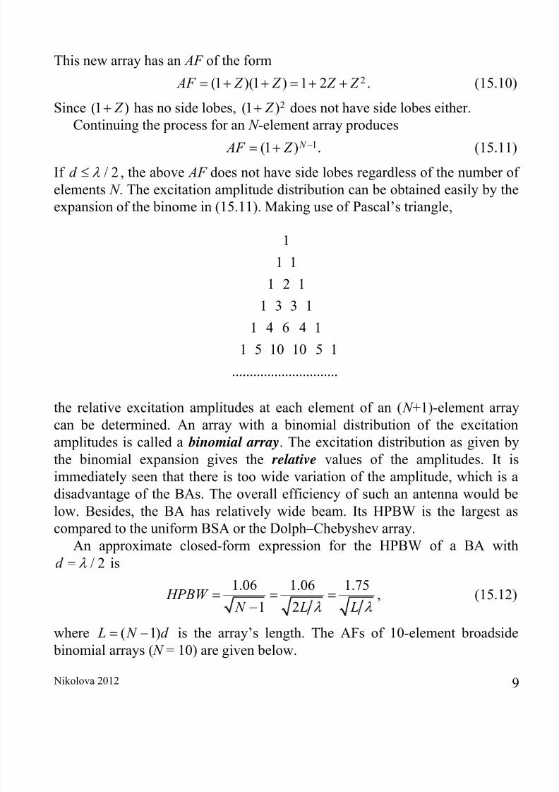
If / 2d , the above AF does not have side lobes regardless of the number ofelements N . The excitation amplitude distribution can be obtained easily by theexpansion of the binome in (15.11). Making use of Pascal’s triangle,

1

1 1

1 2 1

1 3 3 1

1 4 6 4 1

1 5 10 10 5 1

..............................

the relative excitation amplitudes at each element of an ( N +1)-element arraycan be determined. An array with a binomial distribution of the excitationamplitudes is called a binomial array . The excitation distribution as given bythe binomial expansion gives the relative values of the amplitudes. It isimmediately seen that there is too wide variation of the amplitude, which is adisadvantage of the BAs. The overall efficiency of such an antenna would below. Besides, the BA has relatively wide beam. Its HPBW is the largest ascompared to the uniform BSA or the Dolph–Chebyshev array.

An approximate closed-form expression for the HPBW of a BA with/ 2d is

1.06 1.06 1.75

1 2 HPBW

N L L , (15.12)

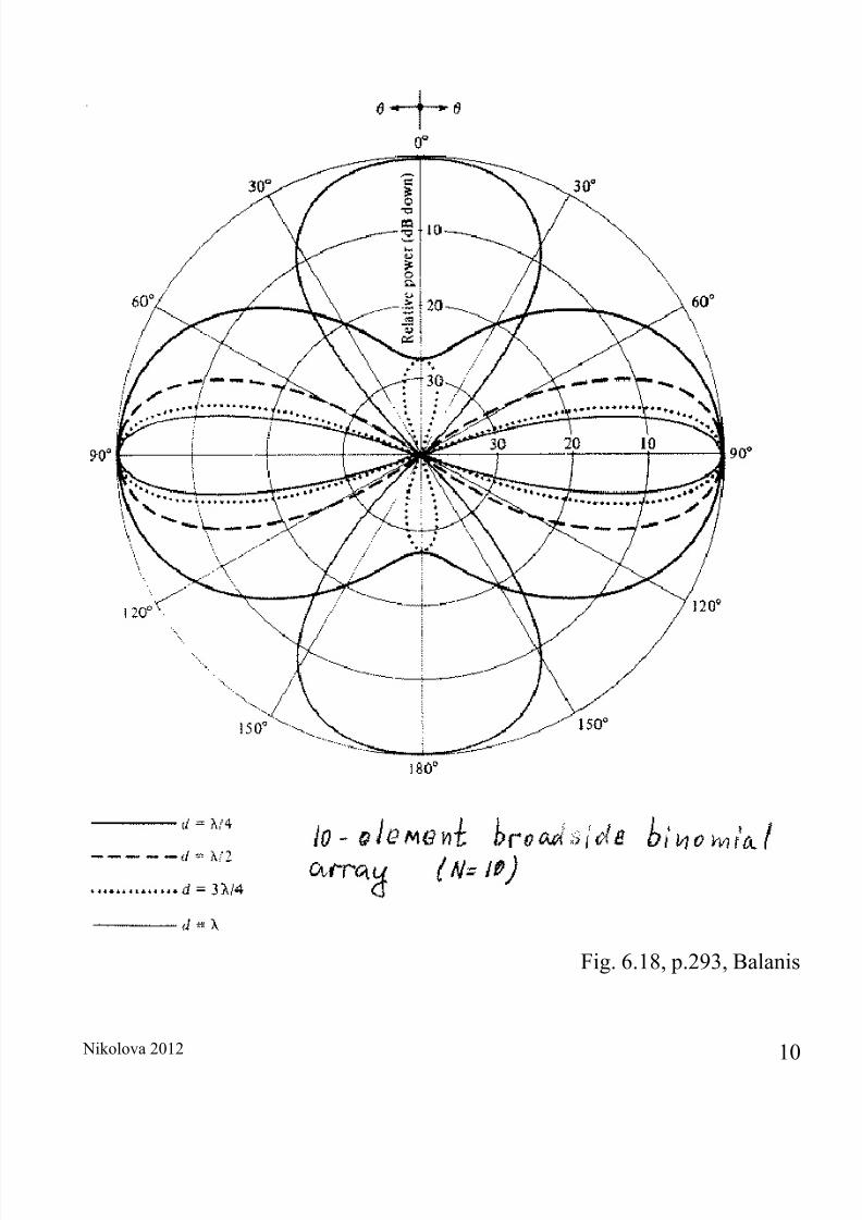
where ( 1) L N d is the array’s length. The AFs of 10-element broadside binomial arrays ( N = 10) are given below.

8/12/2019 L15_Arrays3


Nikolova 2012 10

Fig. 6.18, p.293, Balanis

8/12/2019 L15_Arrays3


Nikolova 2012 11

The directivity of a broadside BA with spacing / 2d can be calculatedas

0 2( 1)

0

2

cos cos2

N D

d

, (15.13)

0(2 2) (2 4) ... 2(2 3) (2 5) ... 1

N N D

N N

, (15.14)

0 1.77 1.77 1 2 D N L . (15.15)

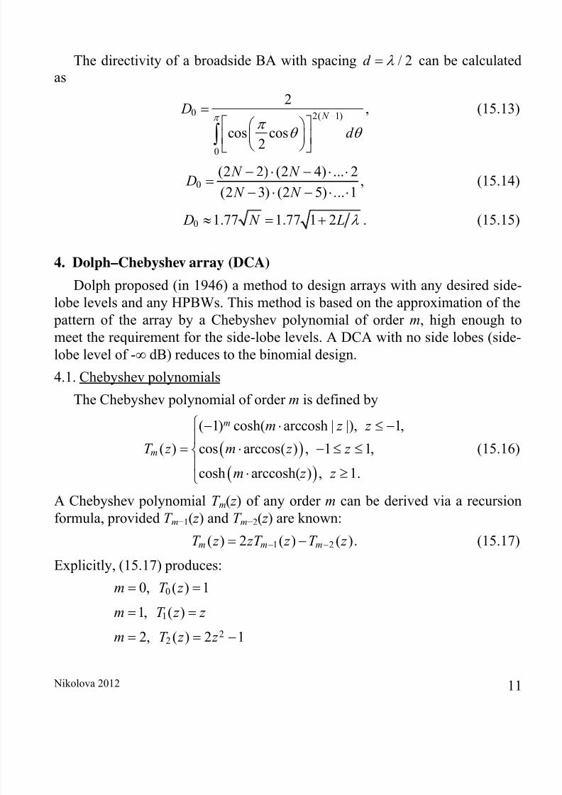
4. Dolph–Chebyshev array (DCA)

Dolph proposed (in 1946) a method to design arrays with any desired side-lobe levels and any HPBWs. This method is based on the approximation of the

pattern of the array by a Chebyshev polynomial of order m, high enough tomeet the requirement for the side-lobe levels. A DCA with no side lobes (side-lobe level of - dB) reduces to the binomial design.

4.1. Chebyshev polynomials

The Chebyshev polynomial of order m is defined by

( 1) cosh( arccosh | |), 1,

( ) cos arccos( ) , 1 1,

cosh arccosh( ) , 1.

m

m

m z z

T z m z z

m z z

(15.16)

A Chebyshev polynomial T m( z ) of any order m can be derived via a recursionformula, provided T m− 1( z ) and T m− 2( z ) are known:

1 2( ) 2 ( ) ( )m m mT z zT z T z . (15.17)

Explicitly, (15.17) produces:

00, ( ) 1m T z

11, ( )m T z z 2

22, ( ) 2 1m T z z

8/12/2019 L15_Arrays3


Nikolova 2012 12

333, ( ) 4 3m T z z z

4 244, ( ) 8 8 1m T z z z

5 355, ( ) 16 20 5 , etc.m T z z z z

If | | 1 z , then the Chebyshev polynomials are related to the cosinefunctions, see (15.16). We can always expand the function cos( mx) as a polynomial of cos( x) of order m, e.g., for 2m ,

2cos 2 2cos 1 x . (15.18)

This can be done by observing that ( ) jx m jmxe e and making use of Euler’sformula to expand the exponents as

(cos sin ) cos( ) sin( )m j x mx j mx . (15.19)

The left side of the equation is then expanded and its real and imaginary partsare equated to those on the right. Similar relations hold for the hyperboliccosine function.

Comparing the trigonometric relation in (15.18) with the expression for2 ( )T z above, we see that the Chebyshev argument z is related to the cosine

argument x by

cos or arccos z x x z . (15.20)

For example, (15.18) can be written as:

2cos(2arccos ) 2 cos(arccos ) 1 z z ,

22cos(2arccos ) 2 1 ( ) z z T z . (15.21)

Properties of the Chebyshev polynomials:

1) All polynomials of any order m pass through the point (1,1).

2) Within the range 1 1 z , the polynomials have values within [–1,1].

3) All nulls occur within 1 1 z .4) The maxima and minima in the [ 1,1] z range have values +1 and –1,

respectively.

5) The higher the order of the polynomial, the steeper the slope for | | 1 z .

8/12/2019 L15_Arrays3


Nikolova 2012 13

Fig. 6.19, pp. 296, Balanis

8/12/2019 L15_Arrays3


Nikolova 2012 14

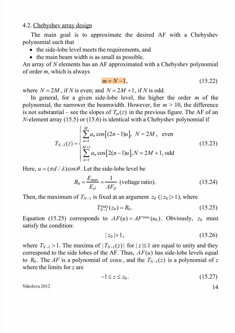
4.2. Chebyshev array design

The main goal is to approximate the desired AF with a Chebyshev polynomial such that

the side-lobe level meets the requirements, and

the main beam width is as small as possible.An array of N elements has an AF approximated with a Chebyshev polynomialof order m, which is always

1m N , (15.22)

where 2 N M , if N is even; and 2 1 N M , if N is odd.In general, for a given side-lobe level, the higher the order m of the

polynomial, the narrower the beamwidth. However, for m > 10, the differenceis not substantial – see the slopes of ( )mT z in the previous figure. The AF of an

N -element array (15.5) or (15.6) is identical with a Chebyshev polynomial if

11 1

1

cos (2 1) , 2 , even

( )

cos 2( 1) , 2 1, odd

M

nn

N M

nn

a n u N M

T z

a n u N M

(15.23)

Here, ( / )cosu d . Let the side-lobe level be

max0

1

sl sl

E R

E AF (voltage ratio). (15.24)

Then, the maximum of 1 N T is fixed at an argument 0 z ( 0| | 1 z ), wheremax

0 01 ( ) N T z R . (15.25)

Equation (15.25) corresponds to max0( ) ( ) F u AF u . Obviously, 0 z must

satisfy the condition:

0| | 1 z , (15.26)

where 1 1 N T . The maxima of 1| ( ) | N T z for | | 1 z are equal to unity and theycorrespond to the side lobes of the AF. Thus, ( ) F u has side-lobe levels equalto 0 R . The AF is a polynomial of cos u , and the 1( ) N T z is a polynomial of z where the limits for z are

01 z z . (15.27)

8/12/2019 L15_Arrays3


Nikolova 2012 15

Since

1 cos 1u , (15.28)

the relation between z and cos u must be normalized as

0cos /u z z . (15.29)

Design of a DCA of N elements – general procedure:

1) Expand the AF as given by (15.5) or (15.6) by replacing each cos( ) mu term ( 1,2,...,m M ) with the power series of cos u .

2) Determine 0 z such that 0 01( ) N T z R (voltage ratio).

3) Substitute 0cos /u z z in the AF as found in step 1.

4) Equate the AF found in Step 3 to 1( ) N T z and determine the coefficientsfor each power of z .

Example: Design a DCA (broadside) of N =10 elements with a major-to-minorlobe ratio of 0 26 R dB. Find the excitation coefficients and form the AF.

Solution:

The order of the Chebyshev polynomial is 1 9m N . The AF for an even-number array is:

5

21

cos (2 1) , cos M nn

d AF a n u u

, 5 .

Step 1: Write 10 F explicitly:

10 1 2 3 4 5cos cos3 cos5 cos7 cos9 F a u a u a u a u a u .

Expand the cos( )mu terms of powers of cos u :3cos3 4cos 3cosu u u ,

5 3cos5 16cos 20cos 5cosu u u u ,7 5 3cos7 64cos 112cos 56cos 7cosu u u u u ,

9 7 5 3cos9 256cos 576cos 432cos 120cos 9cosu u u u u u .

8/12/2019 L15_Arrays3


Nikolova 2012 16

Step 2: Determine 0 z :

0 26 dB R 26

200 10 20 R 9 0( ) 20T z ,

0cosh 9arccosh( ) 20 z ,

09arccosh( ) arccosh20 3.69 z ,0arccosh( ) 0.41 z ,

0 cosh0.41 z 0 1.08515 z .

Step 3: Express the AF from Step 1 in terms of 0cos /u z z :

9

10 1 2 3 4 50

3

2 3 4 530

5

3 4 550

7

4 570

9

590

3 5 7 9

( )

3 5 7 9

4 20 56 120

16 112 432

64 576

256

= 9 120 432 576 256T z

z AF a a a a a

z

z a a a a z

z a a a

z

z a a

z

z a

z z z z z z

Step 4: Finding the coefficients by matching the power terms:9

5 0 5256 256 2.0860a z a 7

4 5 4064 576 576 2.8308a a z a 5

3 4 5 3016 112 432 432 4.1184a a a z a 7

2 3 4 5 204 20 56 120 120 5.2073a a a a z a 9

1 2 3 4 5 103 5 7 9 9 5.8377a a a a a z a

Normalize coefficients with respect to edge element ( N =5):

5 4 3 2 11; 1.357; 1.974; 2.496; 2.789a a a a a

8/12/2019 L15_Arrays3


Nikolova 2012 17

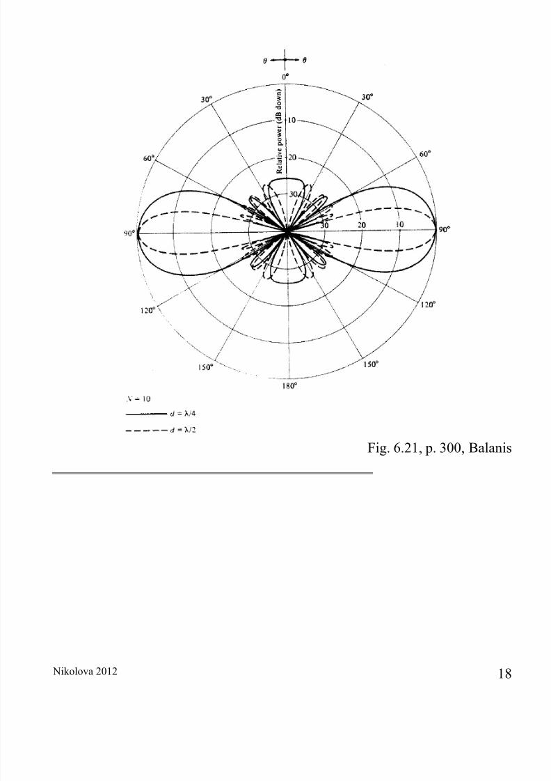
10 2.789cos( ) 2.496cos(3 ) 1.974cos(5 ) 1.357cos(7 ) cos(9 ) F u u u u u

where cosd

u

.

Fig. 6.20b, p. 298, Balanis

8/12/2019 L15_Arrays3


Nikolova 2012 18

Fig. 6.21, p. 300, Balanis

8/12/2019 L15_Arrays3


Nikolova 2012 19

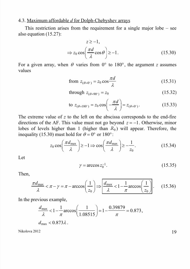
4.3. Maximum affordable d for Dolph-Chebyshev arrays

This restriction arises from the requirement for a single major lobe – seealso equation (15.27):

1 z ,

0 cos cos 1d

z

. (15.30)

For a given array, when varies from 0 to 180 , the argument z assumesvalues

from 0( 0 ) cos d

z z

(15.31)

through 0( 90 ) z z (15.32)

to 0( 180 ) ( 0 )cos d

z z z

. (15.33)

The extreme value of z to the left on the abscissa corresponds to the end-firedirections of the AF. This value must not go beyond 1 z . Otherwise, minorlobes of levels higher than 1 (higher than 0 ) will appear. Therefore, theinequality (15.30) must hold for 0 or 180 :

max max0

0

1cos 1 cosd d z z

. (15.34)

Let1

0arccos z . (15.35)

Then,

max

0

1

arccos

d

z

max

0

1 1

1 arccos

d

z

. (15.36)

In the previous example,

max 1 1 0.398791 arccos 1 0.873

1.08515d

,

max 0.873d .

8/12/2019 L15_Arrays3


Nikolova 2012 20

0

1 z

cos( / )d 1

1

1

maxd

ILLUSTRATION OF EQUATION (15.34) AND THE REQUIREMENT IN (15.36)

5. Directivity of non-uniform arrays

It is difficult to derive closed form expressions for the directivity of non-uniform arrays. Here, we derive expressions in the form of series in the mostgeneral case of a linear array when the excitation coefficients are known.

The non-normalized array factor is1

cos

0

n n

N j jkz

nn

AF a e e , (15.37)

wherena is the amplitude of the excitation of the n-th element;n is the phase angle of the excitation of the n-th element;

n z is the z -coordinate of the n-th element.

The maximum AF is1

max0

N

nn

F a . (15.38)

The normalized AF is1

cos

01

max

0

n n

N j jkz

nn

n N

nn

a e e AF

AF AF

a

. (15.39)

8/12/2019 L15_Arrays3


Nikolova 2012 21

The beam solid angle is derived as

2

0

2 sin A n AF d

,

1 1

( ) cos21 0 0 0

0

2 sinm p m p

N N j jk z z

A m p N m p

nn

a a e e d

a

, (15.40)

where

cos

0

2sin ( )sin

( )m p

m p jk z z

m p

k z z e d

k z z

.

1 1

21 0 0

0

sin ( )4( )

m p

N N m p j

A m p N m pm p

nn

k z z a a e

k z z a

. (15.41)

From

04

A D

,

we obtain

21

00 1 1

0 0

sin ( )

( )m p

N

nn

N N m p j

m pm pm p

a

Dk z z

a a ek z z

. (15.42)

For equispaced linear ( n z nd ) arrays, (15.42) reduces to

21

00 1 1

0 0

sin ( )( )

m p

N

nn

N N j

m pm p

a

Dm p kd

a a em p kd

. (15.43)

8/12/2019 L15_Arrays3


Nikolova 2012 22

For equispaced broadside arrays, where m p for any ( m, p), (15.43)reduces to

21

00 1 1

0 0

sin ( )( )

N

nn

N N

m pm p

a

D m p kd a a

m p kd

. (15.44)

For equispaced broadside uniform arrays,

2

0 1 1

0 0

sin ( )( )

N N

m p

N D

m p kd m p kd

. (15.45)

When the spacing d is a multiple of / 2 , equation (15.44) reduces to21

00 1

2

0

, , ,...2

( )

N

nn

N

nn

a

D d a

. (15.46)

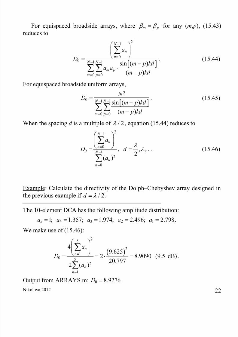
Example: Calculate the directivity of the Dolph–Chebyshev array designed inthe previous example if / 2d .

The 10-element DCA has the following amplitude distribution:

5 4 3 2 11; 1.357; 1.974; 2.496; 2.798a a a a a .

We make use of (15.46):

25

21

0 52

1

49.625

2 8.9090 (9.5 dB)20.797

2 ( )

nn

nn

a

Da

.

Output from ARRAYS.m: 0 8.9276 D .

8/12/2019 L15_Arrays3


6. Half-power beamwidth of a BS DCA

For large DCA with side lobes in the range from –20 dB to –60 dB, theHPBW can be found by introducing a beam-broadening factor f given by

2

2 200

21 0.636 cosh (arccosh ) f R R

. (15.47)

The HPBW of the DCA is equal to the product of the broadening factor by theHPBW of the respective uniform linear array:

DCA UA PBW f HPBW . (15.48)

In (15.47), 0 R denotes the side-lobe level (voltage ratio).

Documents

L15_Arrays3