Embed Size (px)
Citation preview
DSA - lecture 6 - T.U.Cluj-Napoca - M. Joldos 1
Terminology. Free Trees. Representations. Minimum Spanning Trees (algorithms: Prim, Kruskal). Graph Traversals (dfs, bfs). Articulation points & BiconnectedComponents. Graph Matching
Undirected Graphs
DSA - lecture 6 - T.U.Cluj-Napoca - M. Joldos 2
� Graphs provide a useful way to model a large variety of problems in an abstract way• Communication networks• Computer networks• Maps (cities and highways)• Path planning in AI (states and moves)• Scientific taxonomy• Activity charts (tasks and dependencies)• Flow chart of computer programs
Application domains for graphs
DSA - lecture 6 - T.U.Cluj-Napoca - M. Joldos 3
� Undirected graphs (or just graphs): G=(V, E), with Vand E finite (true for digraphs as well)• Differ from digraphs by the fact that each edge is unordered
(i.e. (u, v) is the same as (v, u))
� Visualizations of graphs (and digraphs) are usually embeddings
� An embedding maps each node of G to a point in the plane, and each arc to a curve or straight line segment between two vertices
� Planar graph: has an embedding where no two edges cross• One graph may have many embeddings
Undirected graphs
DSA - lecture 6 - T.U.Cluj-Napoca - M. Joldos 4
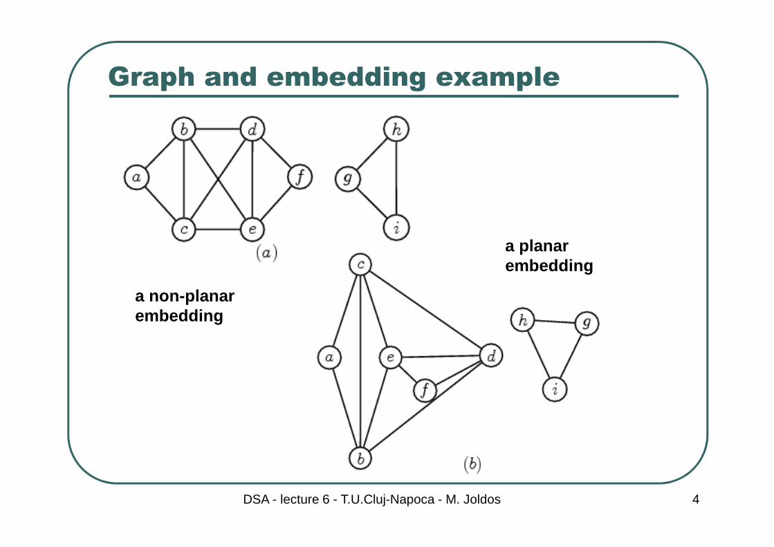
Graph and embedding example
a non-planar embedding
a planar embedding

DSA - lecture 6 - T.U.Cluj-Napoca - M. Joldos 5
Other graph visualizations
DSA - lecture 6 - T.U.Cluj-Napoca - M. Joldos 6
Graph terminology
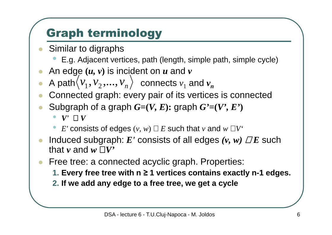
� Similar to digraphs• E.g. Adjacent vertices, path (length, simple path, simple cycle)
� An edge (u, v) is incident on u and v� A path connects v1 and vn
� Connected graph: every pair of its vertices is connected� Subgraph of a graph G=(V, E): graph G’=(V’, E’ )
• V' ⊆⊆⊆⊆ V• E' consists of edges (v, w) ∈ E such that v and w ∈V‘
� Induced subgraph: E' consists of all edges (v, w) ∈∈∈∈ E such that v and w ∈∈∈∈V’
� Free tree: a connected acyclic graph. Properties:1. Every free tree with n ≥ 1 vertices contains exactly n-1 edges.2. If we add any edge to a free tree, we get a cycle
nvvv ,...,, 21
DSA - lecture 6 - T.U.Cluj-Napoca - M. Joldos 7
Free tree properties
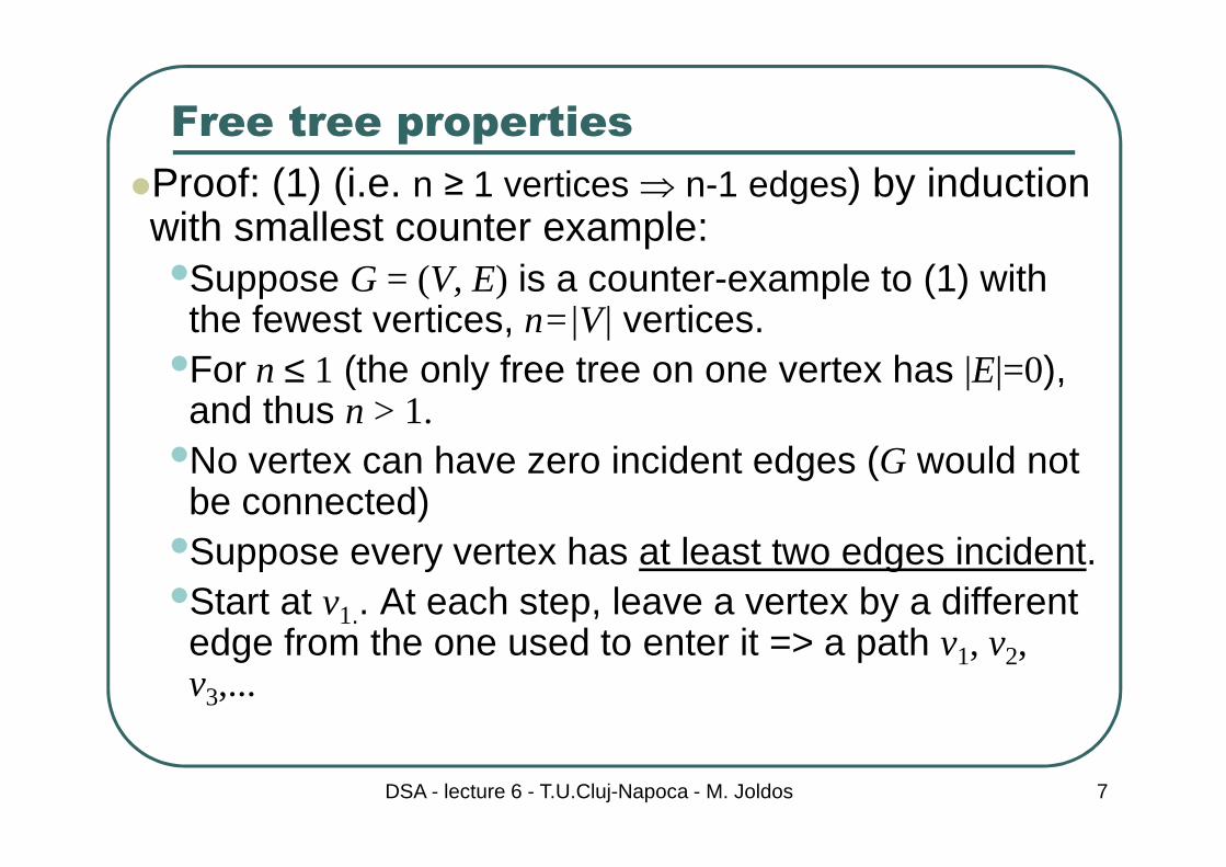
�Proof: (1) (i.e. n ≥ 1 vertices ⇒ n-1 edges) by induction with smallest counter example:•Suppose G = (V, E) is a counter-example to (1) with the fewest vertices, n=|V| vertices.
•For n ≤ 1 (the only free tree on one vertex has |E|=0), and thus n > 1.
•No vertex can have zero incident edges (G would not be connected)
•Suppose every vertex has at least two edges incident. •Start at v1.. At each step, leave a vertex by a different edge from the one used to enter it => a path v1, v2, v3,...
DSA - lecture 6 - T.U.Cluj-Napoca - M. Joldos 8
Free tree properties. Proof (cont’d)
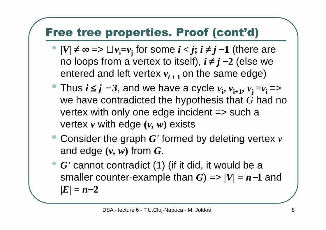
• |V| ≠≠≠≠ ∞∞∞∞ => ∃ vi=vj for some i < j; i ≠≠≠≠ j −−−−1 (there are no loops from a vertex to itself), i ≠≠≠≠ j −−−−2 (else we entered and left vertex vi + 1 on the same edge)
• Thus i ≤≤≤≤ j −−−− 3, and we have a cycle vi, vi+1, vj =vi =>we have contradicted the hypothesis that G had no vertex with only one edge incident => such a vertex v with edge (v, w) exists
• Consider the graph G' formed by deleting vertex vand edge (v, w) from G.
• G' cannot contradict (1) (if it did, it would be a smaller counter-example than G) => |V| = n−−−−1 and |E| = n−−−−2

DSA - lecture 6 - T.U.Cluj-Napoca - M. Joldos 9
Free tree properties. Proof (cont’d)
• But G has |V|=|V’|+1 and |E|=|E’|+1 => G has n-1 edges (proving that G does indeed satisfy (1))
• No smallest counter-example to (1); we conclude there can be no counter-example at all, so (1) is true.
� For (2) (adding an edge to a free tree forms a cycle)• Assume it does not for a cycle=> adding the edge to a
free tree of n vertices would be a graph with n vertices and n edges, connected, and we supposed that adding the edge left the graph acyclic. Thus we would have a free tree whose vertex and edge count did not satisfy condition (1)(i.e. contains exactly n−1 edges)
DSA - lecture 6 - T.U.Cluj-Napoca - M. Joldos 10
Methods of representation for graphs
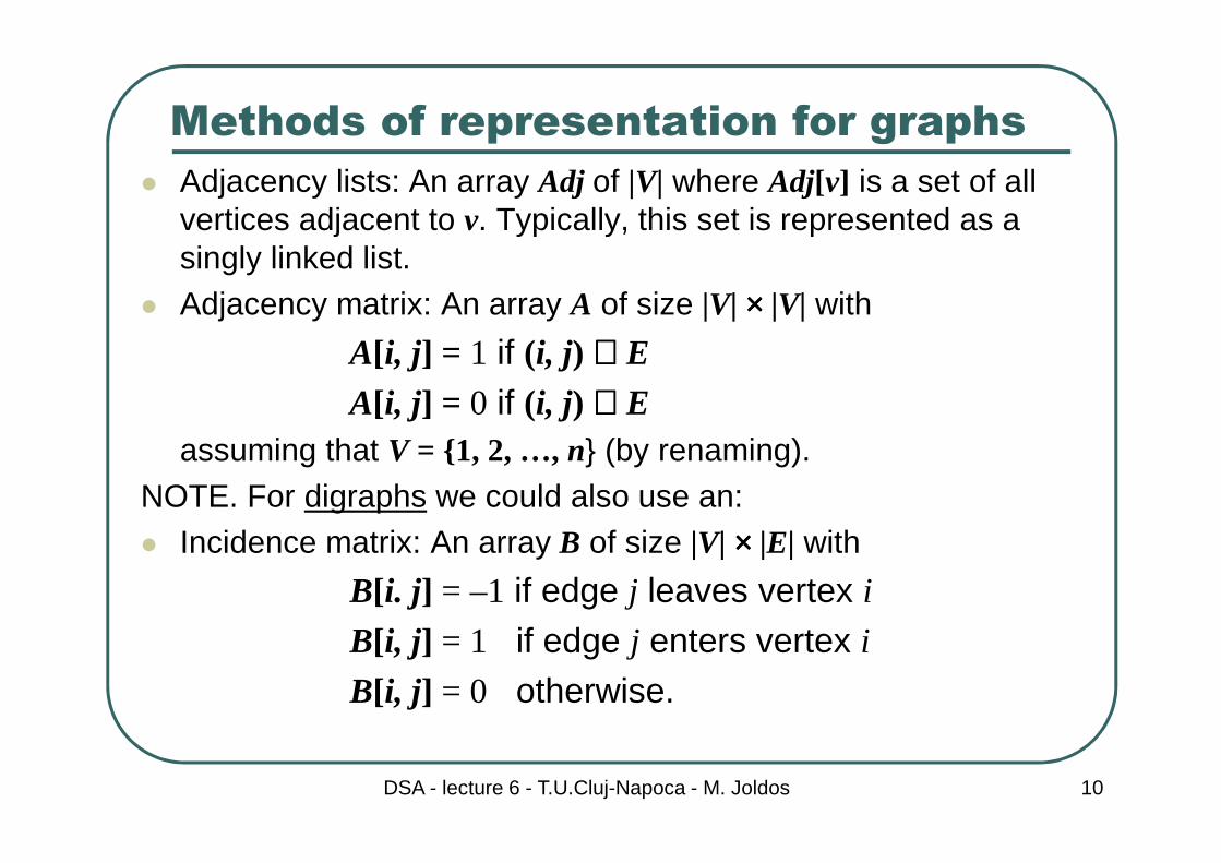
� Adjacency lists: An array Adj of |V| where Adj[v] is a set of all vertices adjacent to v. Typically, this set is represented as a singly linked list.
� Adjacency matrix: An array A of size |V| ×××× |V| with
A[i, j] = 1 if (i, j) ∈∈∈∈ E
A[i, j] = 0 if (i, j) ∉∉∉∉ Eassuming that V = {1, 2, …, n} (by renaming).
NOTE. For digraphs we could also use an:� Incidence matrix: An array B of size |V| ×××× |E| with
B[i. j] = –1 if edge j leaves vertex iB[i, j] = 1 if edge j enters vertex iB[i, j] = 0 otherwise.
DSA - lecture 6 - T.U.Cluj-Napoca - M. Joldos 11
Sparse and dense graphs
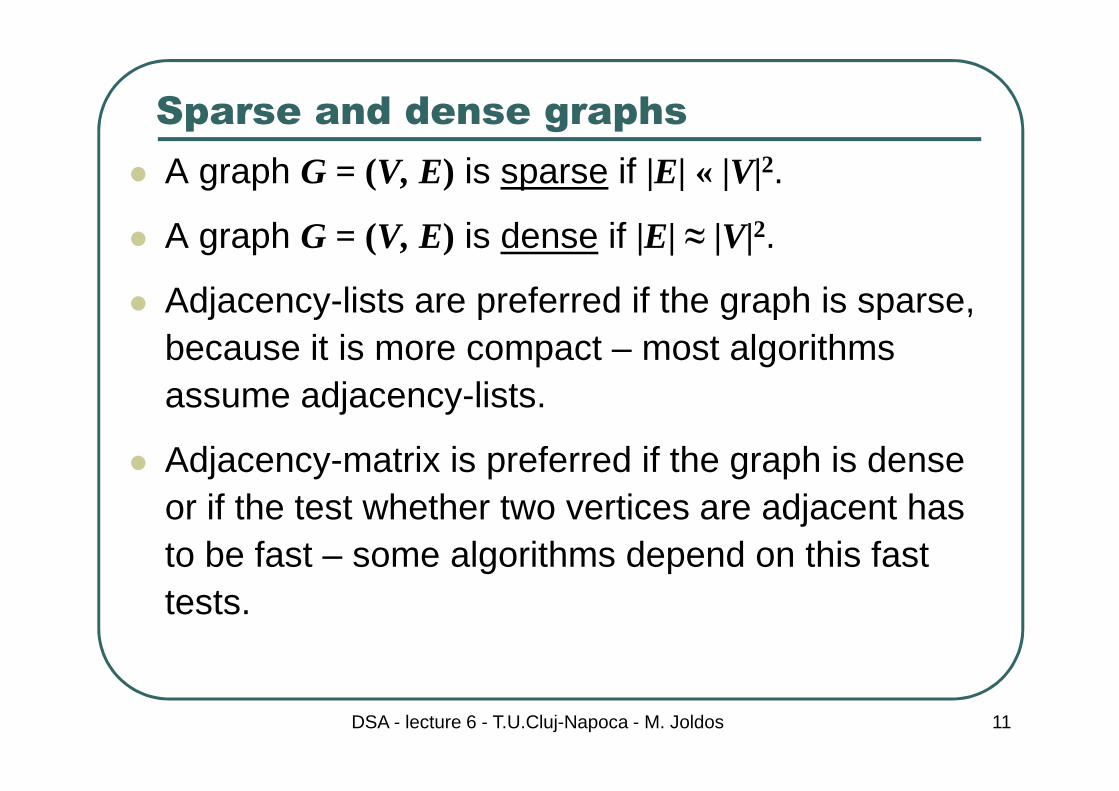
� A graph G = (V, E) is sparse if |E| « |V|2.
� A graph G = (V, E) is dense if |E| ≈ |V|2.
� Adjacency-lists are preferred if the graph is sparse, because it is more compact – most algorithms assume adjacency-lists.
� Adjacency-matrix is preferred if the graph is denseor if the test whether two vertices are adjacent has to be fast – some algorithms depend on this fast tests.
DSA - lecture 6 - T.U.Cluj-Napoca - M. Joldos 12
The minimum cost spanning tree (MST)
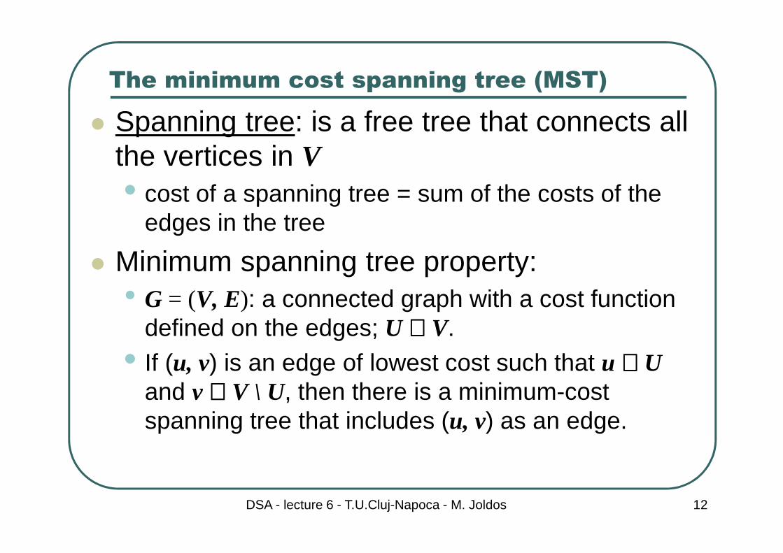
� Spanning tree: is a free tree that connects all the vertices in V• cost of a spanning tree = sum of the costs of the
edges in the tree
� Minimum spanning tree property: • G = (V, E): a connected graph with a cost function
defined on the edges; U ⊆⊆⊆⊆ V. • If (u, v) is an edge of lowest cost such that u ∈∈∈∈ U
and v ∈∈∈∈ V \ U, then there is a minimum-cost spanning tree that includes (u, v) as an edge.
DSA - lecture 6 - T.U.Cluj-Napoca - M. Joldos 13
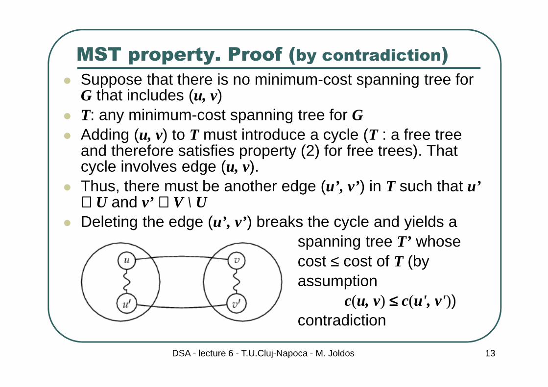
� Suppose that there is no minimum-cost spanning tree for G that includes (u, v)
� T: any minimum-cost spanning tree for G� Adding (u, v) to T must introduce a cycle (T : a free tree
and therefore satisfies property (2) for free trees). That cycle involves edge (u, v).
� Thus, there must be another edge (u’, v’ ) in T such that u’ ∈∈∈∈ U and v’ ∈∈∈∈ V \ U
� Deleting the edge (u’, v’ ) breaks the cycle and yields aspanning tree T’ whosecost ≤ cost of T (byassumption
c(u, v) ≤≤≤≤ c(u', v')) contradiction
MST property. Proof (by contradiction)
DSA - lecture 6 - T.U.Cluj-Napoca - M. Joldos 14
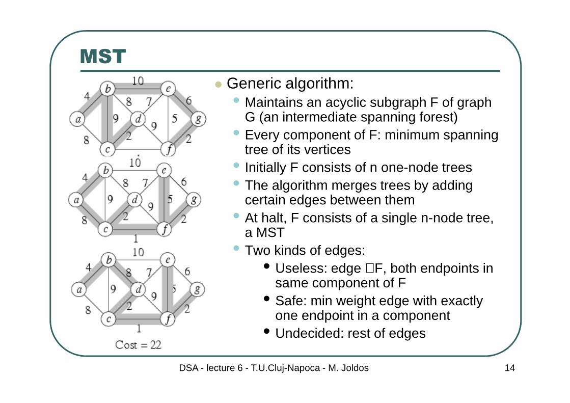
� Generic algorithm:• Maintains an acyclic subgraph F of graph
G (an intermediate spanning forest)• Every component of F: minimum spanning
tree of its vertices• Initially F consists of n one-node trees• The algorithm merges trees by adding
certain edges between them• At halt, F consists of a single n-node tree,
a MST• Two kinds of edges:
• Useless: edge ∉F, both endpoints in same component of F
• Safe: min weight edge with exactly one endpoint in a component
• Undecided: rest of edges
MST
DSA - lecture 6 - T.U.Cluj-Napoca - M. Joldos 15
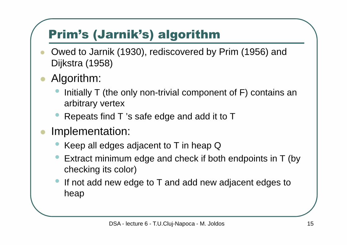
� Owed to Jarnik (1930), rediscovered by Prim (1956) and Dijkstra (1958)
� Algorithm:• Initially T (the only non-trivial component of F) contains an
arbitrary vertex• Repeats find T ’s safe edge and add it to T
� Implementation:• Keep all edges adjacent to T in heap Q• Extract minimum edge and check if both endpoints in T (by
checking its color)• If not add new edge to T and add new adjacent edges to
heap
Prim’s (Jarnik’s) algorithm
DSA - lecture 6 - T.U.Cluj-Napoca - M. Joldos 16
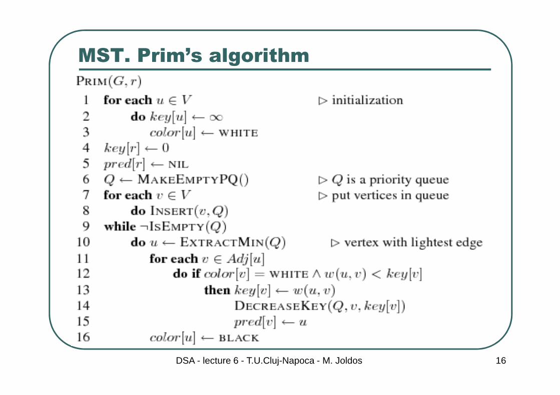
MST. Prim’s algorithm
DSA - lecture 6 - T.U.Cluj-Napoca - M. Joldos 17
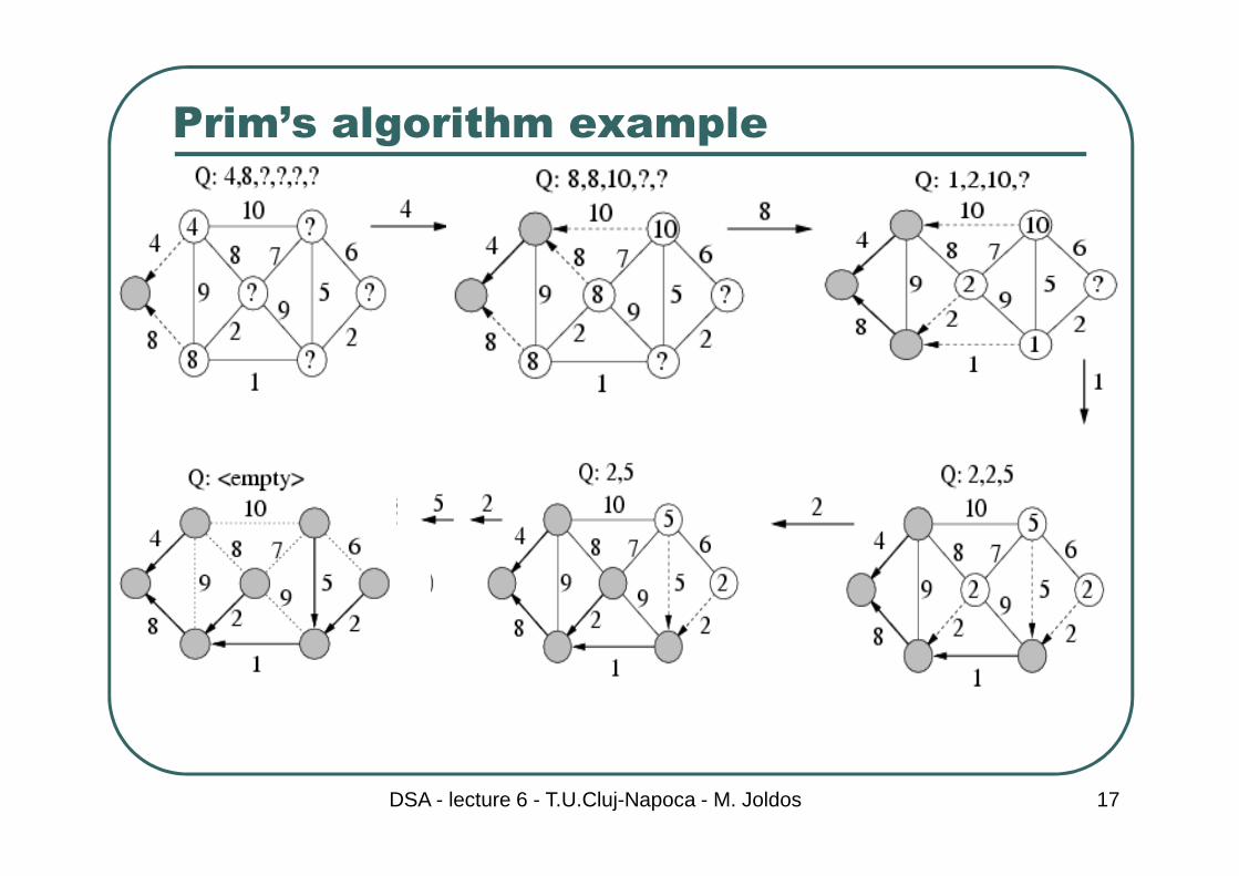
Prim’s algorithm example
DSA - lecture 6 - T.U.Cluj-Napoca - M. Joldos 18
� Running time• Dominated by the cost of the heap operations:
insert, extractMin and DecreaseKey
• Insert and extractMin are called O(|V|=n) times (once per vertex, except r)
• operations mentioned before can be performed in O(log n) time, for a heap of n items
MST. Prim’s algorithm
DSA - lecture 6 - T.U.Cluj-Napoca - M. Joldos 19
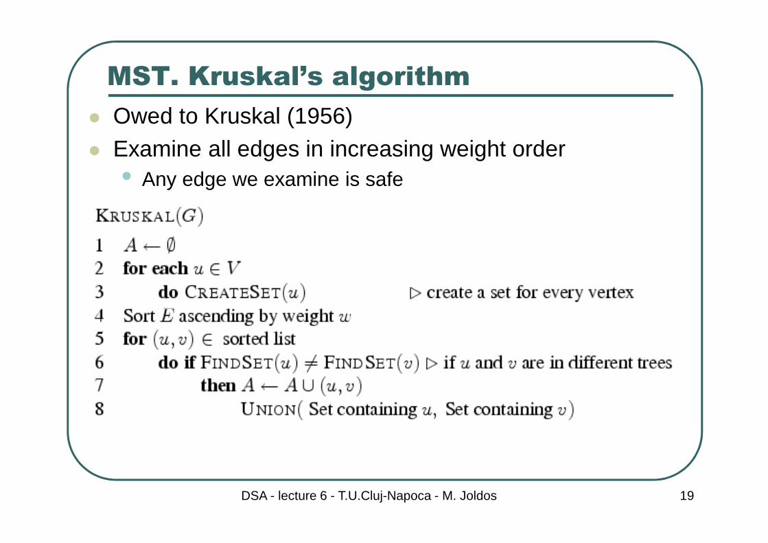
� Owed to Kruskal (1956)� Examine all edges in increasing weight order
• Any edge we examine is safe
MST. Kruskal’s algorithm
DSA - lecture 6 - T.U.Cluj-Napoca - M. Joldos 20
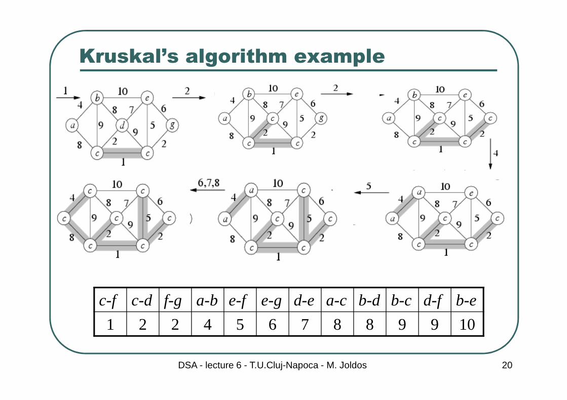
Kruskal’s algorithm example
c-f c-d f-g a-b e-f e-g d-e a-c b-d b-c d-f b-e
1 2 2 4 5 6 7 8 8 9 9 10
DSA - lecture 6 - T.U.Cluj-Napoca - M. Joldos 21
Animations of Prim's and Kruskal's
Algorithms
� http://www.unf.edu/~wkloster/foundations/PrimApplet/PrimApplet.htm
� http://students.ceid.upatras.gr/%7Epapagel/project/prim.htm
� http://www.math.ucsd.edu/~fan/algo/CS101.swf
DSA - lecture 6 - T.U.Cluj-Napoca - M. Joldos 22
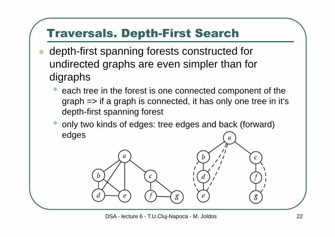
� depth-first spanning forests constructed for undirected graphs are even simpler than for digraphs• each tree in the forest is one connected component of the
graph => if a graph is connected, it has only one tree in it's depth-first spanning forest
• only two kinds of edges: tree edges and back (forward) edges
Traversals. Depth-First Search
DSA - lecture 6 - T.U.Cluj-Napoca - M. Joldos 23
Breadth-First Search (BFS)
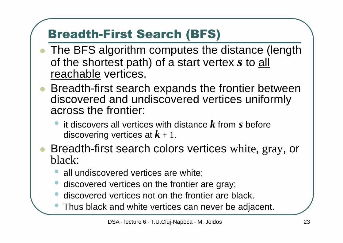
� The BFS algorithm computes the distance (length of the shortest path) of a start vertex s to all reachable vertices.
� Breadth-first search expands the frontier between discovered and undiscovered vertices uniformly across the frontier: • it discovers all vertices with distance k from sbefore
discovering vertices at k + 1.
� Breadth-first search colors vertices white, gray, or black:• all undiscovered vertices are white;• discovered vertices on the frontier are gray;• discovered vertices not on the frontier are black.• Thus black and white vertices can never be adjacent.
DSA - lecture 6 - T.U.Cluj-Napoca - M. Joldos 24
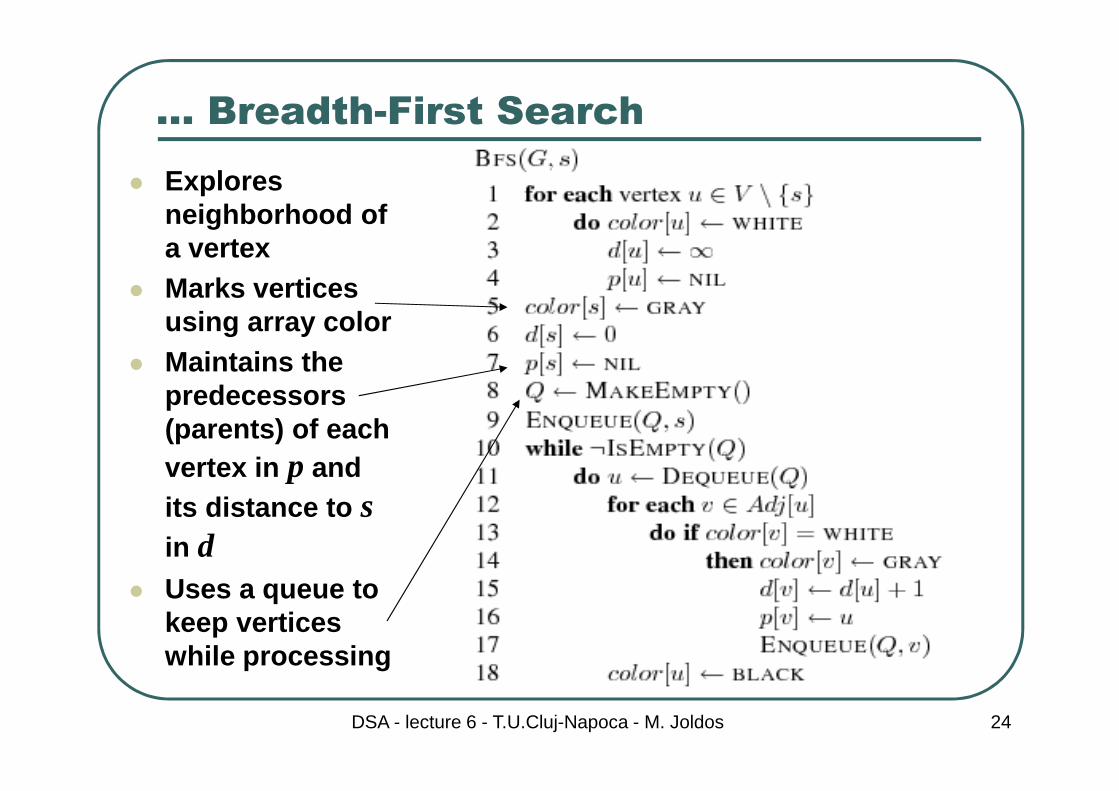
… Breadth-First Search
� Explores neighborhood of a vertex
� Marks vertices using array color
� Maintains the predecessors (parents) of each vertex in p and its distance to sin d
� Uses a queue to keep vertices while processing
DSA - lecture 6 - T.U.Cluj-Napoca - M. Joldos 25
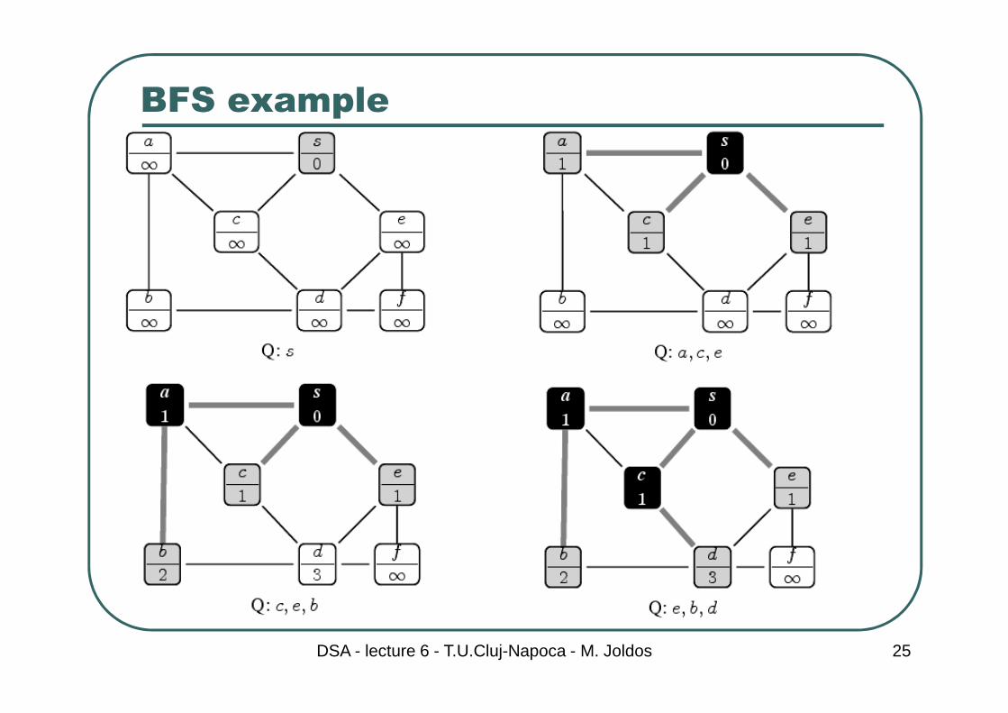
BFS example
DSA - lecture 6 - T.U.Cluj-Napoca - M. Joldos 26
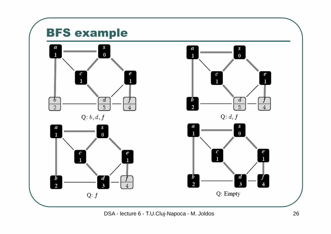
BFS example
DSA - lecture 6 - T.U.Cluj-Napoca - M. Joldos 27
Analysis of BFS
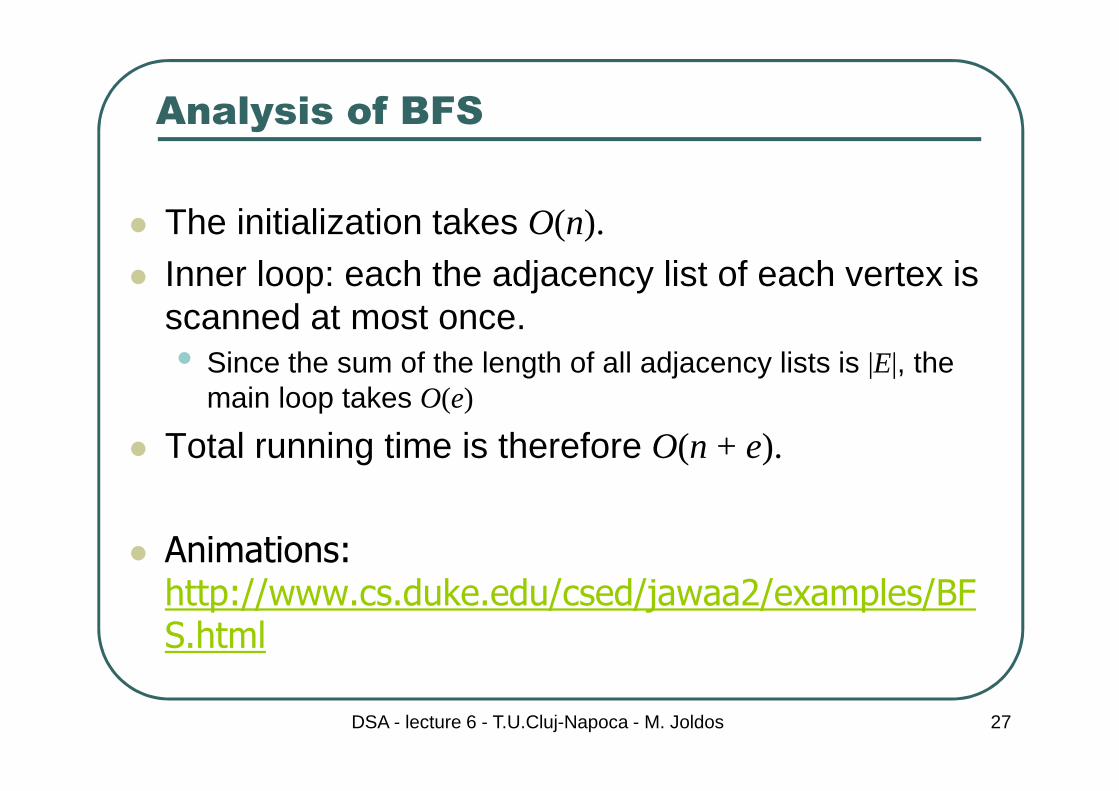
� The initialization takes O(n).
� Inner loop: each the adjacency list of each vertex is scanned at most once. • Since the sum of the length of all adjacency lists is |E|, the
main loop takes O(e)
� Total running time is therefore O(n + e).
� Animations: http://www.cs.duke.edu/csed/jawaa2/examples/BFS.html
DSA - lecture 6 - T.U.Cluj-Napoca - M. Joldos 28
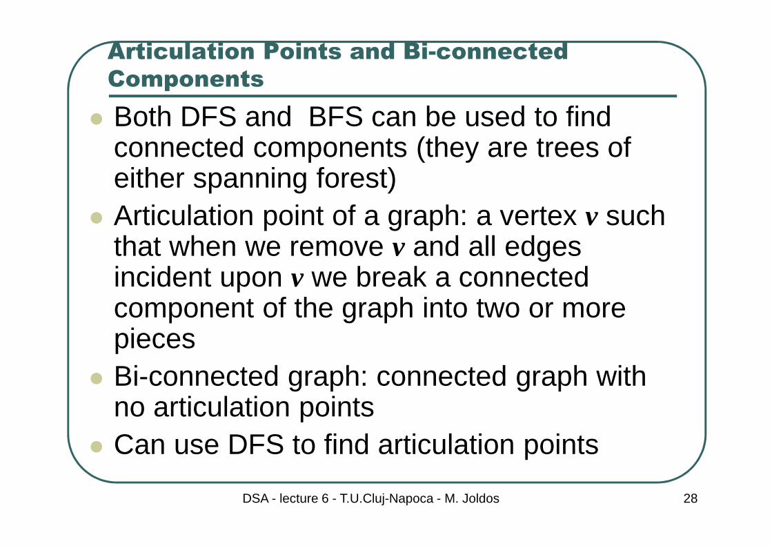
� Both DFS and BFS can be used to find connected components (they are trees of either spanning forest)
� Articulation point of a graph: a vertex v such that when we remove v and all edges incident upon v we break a connected component of the graph into two or more pieces
� Bi-connected graph: connected graph with no articulation points
� Can use DFS to find articulation points
Articulation Points and Bi-connected
Components
DSA - lecture 6 - T.U.Cluj-Napoca - M. Joldos 29
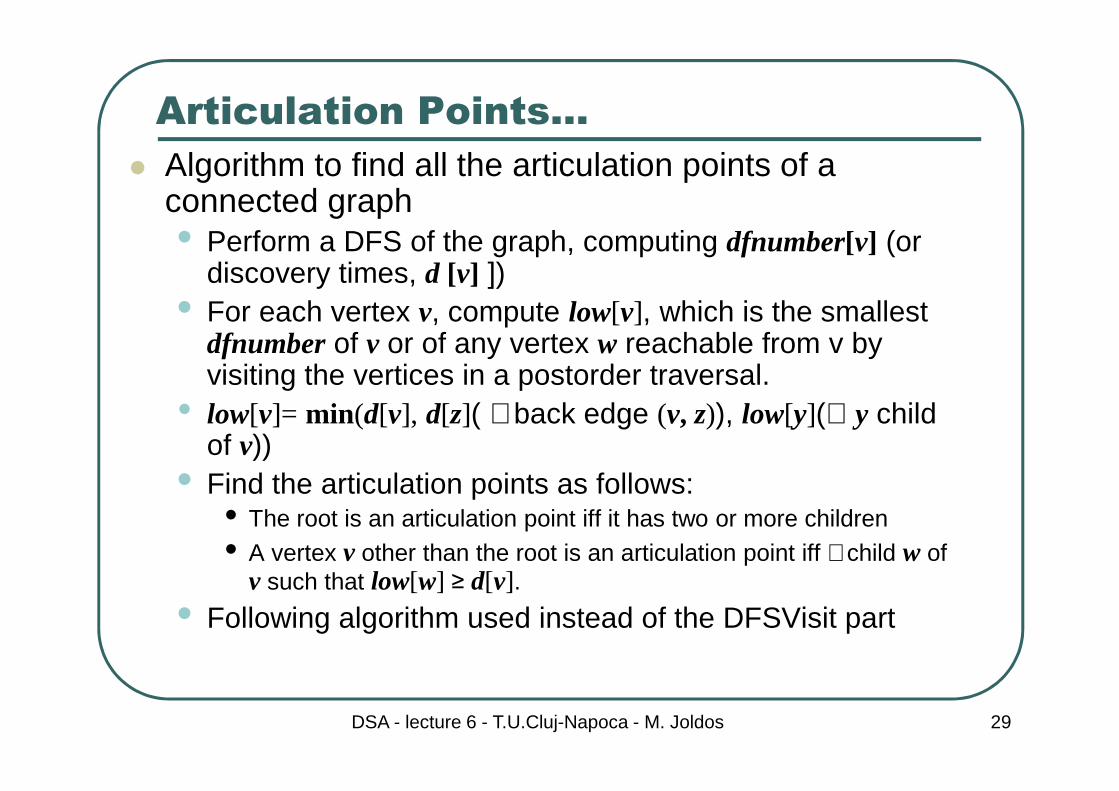
� Algorithm to find all the articulation points of a connected graph• Perform a DFS of the graph, computing dfnumber[v] (or
discovery times, d [v] ])• For each vertex v, compute low[v], which is the smallest
dfnumberof v or of any vertex w reachable from v by visiting the vertices in a postorder traversal.
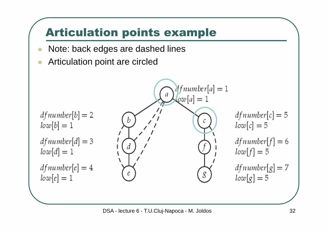
• low[v]= min(d[v], d[z]( ∃ back edge (v, z)), low[y](∀ y child of v))
• Find the articulation points as follows:• The root is an articulation point iff it has two or more children• A vertex v other than the root is an articulation point iff ∃ child w of
v such that low[w] ≥ d[v].
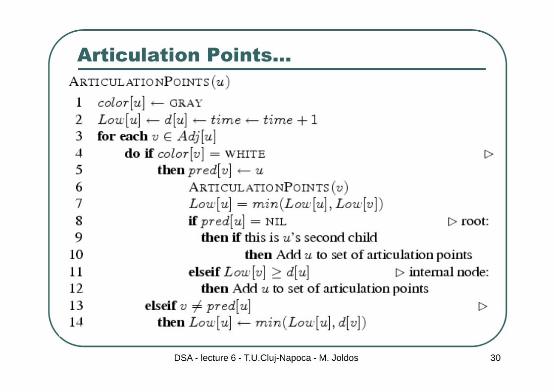
• Following algorithm used instead of the DFSVisit part
Articulation Points…
DSA - lecture 6 - T.U.Cluj-Napoca - M. Joldos 30
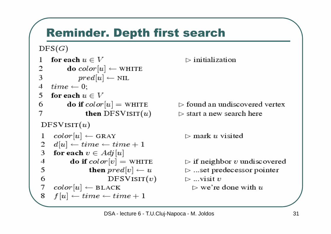
Articulation Points…
DSA - lecture 6 - T.U.Cluj-Napoca - M. Joldos 31
Reminder. Depth first search
DSA - lecture 6 - T.U.Cluj-Napoca - M. Joldos 32
� Note: back edges are dashed lines� Articulation point are circled
Articulation points example
DSA - lecture 6 - T.U.Cluj-Napoca - M. Joldos 33
� Bipartite graph: its vertices can be divided into two disjoint groups with each edge having one end in each group
� Matching: given a graph G=(V, E), a subset of the edges in E with no two edges incident upon the same vertex in V
� Maximum cardinality matching problem: the task of selecting a maximum subset of such edges (maximal matching)
� Complete matching: matching in which every vertex is an endpoint of some edge in the matching
Graph matching
DSA - lecture 6 - T.U.Cluj-Napoca - M. Joldos 34
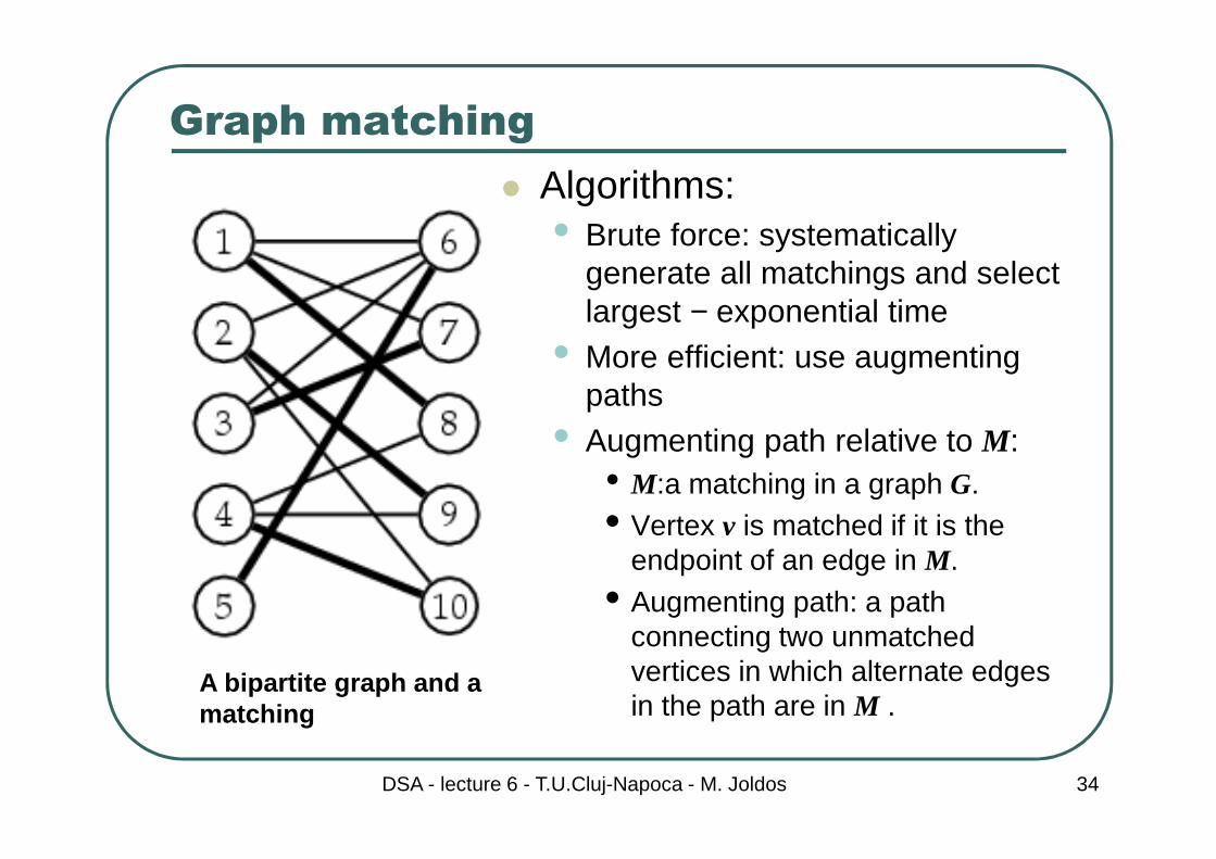
� Algorithms:• Brute force: systematically
generate all matchings and select largest − exponential time
• More efficient: use augmenting paths
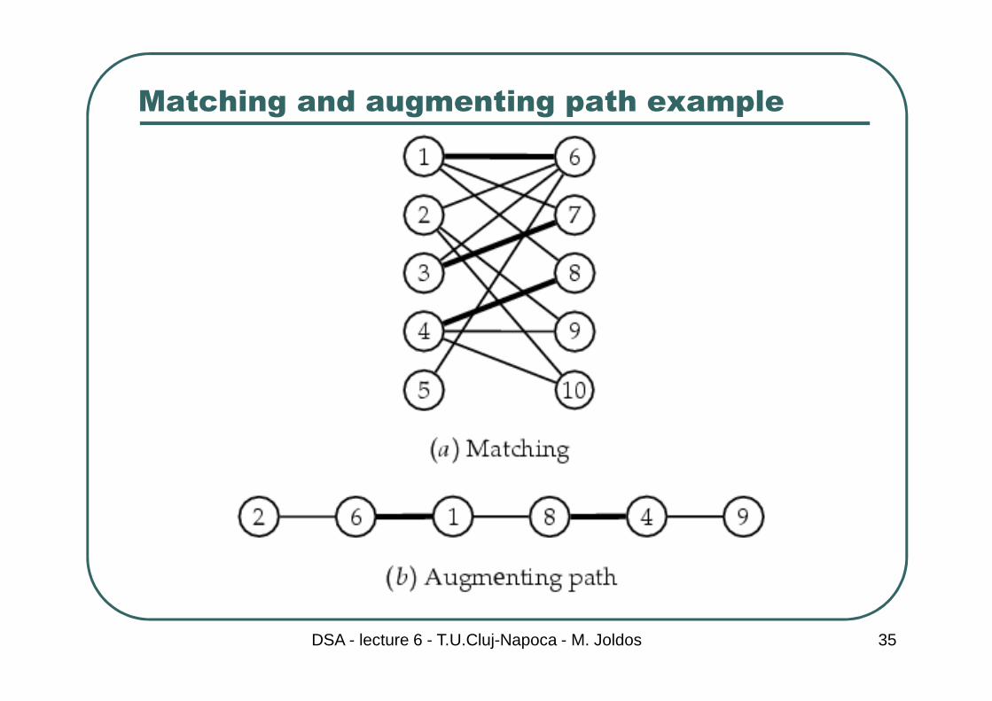
• Augmenting path relative to M:• M:a matching in a graph G. • Vertex v is matched if it is the
endpoint of an edge in M. • Augmenting path: a path
connecting two unmatched vertices in which alternate edges in the path are in M .
Graph matching
A bipartite graph and a matching
DSA - lecture 6 - T.U.Cluj-Napoca - M. Joldos 35
Matching and augmenting path example
DSA - lecture 6 - T.U.Cluj-Napoca - M. Joldos 36
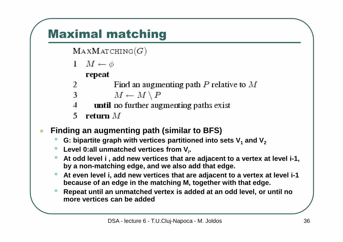
� Finding an augmenting path (similar to BFS)• G: bipartite graph with vertices partitioned into sets V1 and V2
• Level 0:all unmatched vertices from Vi. • At odd level i , add new vertices that are adjacent to a vertex at level i-1,
by a non-matching edge, and we also add that edge.• At even level i, add new vertices that are adjacent to a vertex at level i-1
because of an edge in the matching M, together with that edge.• Repeat until an unmatched vertex is added at an odd level, or until no
more vertices can be added
Maximal matching
DSA - lecture 6 - T.U.Cluj-Napoca - M. Joldos 37
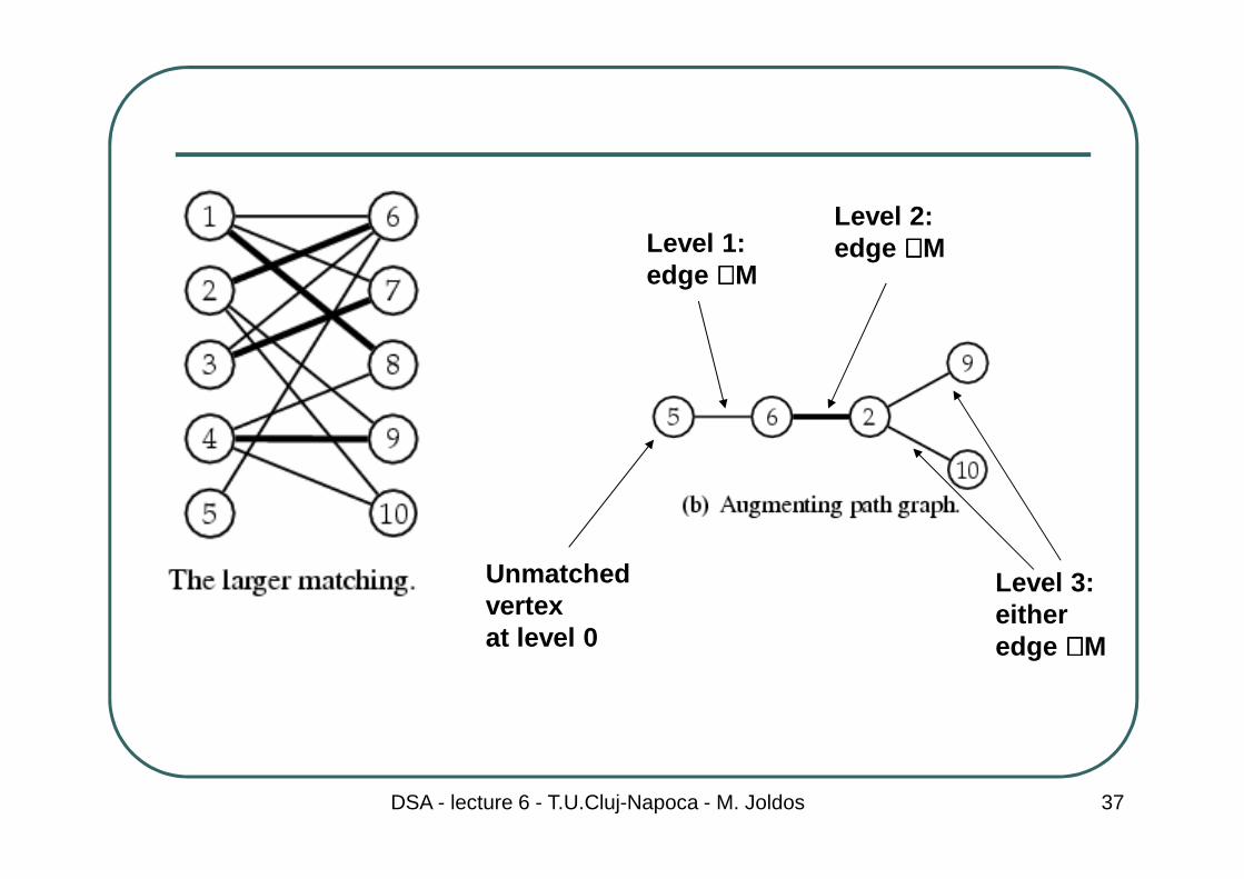
Unmatched vertexat level 0
Level 1: edge ∉∉∉∉M
Level 2: edge ∈∈∈∈M
Level 3: eitheredge ∉∉∉∉M
DSA - lecture 6 - T.U.Cluj-Napoca - M. Joldos 38
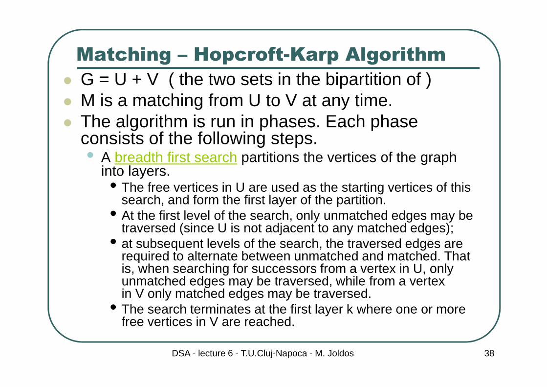
Matching – Hopcroft-Karp Algorithm
� G = U + V ( the two sets in the bipartition of )� M is a matching from U to V at any time.� The algorithm is run in phases. Each phase
consists of the following steps.• A breadth first search partitions the vertices of the graph
into layers. • The free vertices in U are used as the starting vertices of this
search, and form the first layer of the partition. • At the first level of the search, only unmatched edges may be
traversed (since U is not adjacent to any matched edges); • at subsequent levels of the search, the traversed edges are
required to alternate between unmatched and matched. That is, when searching for successors from a vertex in U, only unmatched edges may be traversed, while from a vertex in V only matched edges may be traversed.
• The search terminates at the first layer k where one or more free vertices in V are reached.
DSA - lecture 6 - T.U.Cluj-Napoca - M. Joldos 39
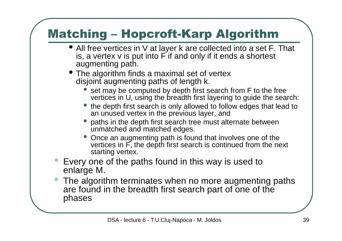
Matching – Hopcroft-Karp Algorithm• All free vertices in V at layer k are collected into a set F. That
is, a vertex v is put into F if and only if it ends a shortest augmenting path.
• The algorithm finds a maximal set of vertex disjoint augmenting paths of length k.
• set may be computed by depth first search from F to the free vertices in U, using the breadth first layering to guide the search:
• the depth first search is only allowed to follow edges that lead to an unused vertex in the previous layer, and
• paths in the depth first search tree must alternate between unmatched and matched edges.
• Once an augmenting path is found that involves one of the vertices in F, the depth first search is continued from the next starting vertex.
• Every one of the paths found in this way is used to enlarge M.
• The algorithm terminates when no more augmenting paths are found in the breadth first search part of one of the phases
DSA - lecture 6 - T.U.Cluj-Napoca - M. Joldos 40
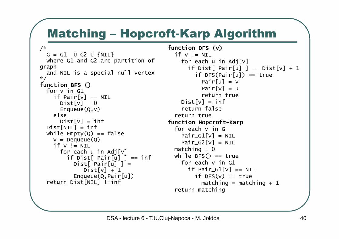
Matching – Hopcroft-Karp Algorithm/* G = G1 U G2 U {NIL}where G1 and G2 are partition of
graphand NIL is a special null vertex
*/function BFS ()function BFS ()function BFS ()function BFS ()for v in G1if Pair[v] == NIL Dist[v] = 0Enqueue(Q,v)
elseDist[v] = inf
Dist[NIL] = infwhile Empty(Q) == false v = Dequeue(Q)if v != NIL for each u in Adj[v] if Dist[ Pair[u] ] == inf Dist[ Pair[u] ] =
Dist[v] + 1Enqueue(Q,Pair[u])
return Dist[NIL] !=inf
function DFS (v) function DFS (v) function DFS (v) function DFS (v) if v != NIL for each u in Adj[v] if Dist[ Pair[u] ] == Dist[v] + 1 if DFS(Pair[u]) == true Pair[u] = vPair[v] = ureturn true
Dist[v] = infreturn false
return truefunction Hopcroftfunction Hopcroftfunction Hopcroftfunction Hopcroft----Karp Karp Karp Karp for each v in G Pair_G1[v] = NIL Pair_G2[v] = NIL
matching = 0 while BFS() == true for each v in G1if Pair_G1[v] == NIL if DFS(v) == true matching = matching + 1
return matching
The Marriage Problem and Matchings
DSA - lecture 6 - T.U.Cluj-Napoca - M. Joldos 41
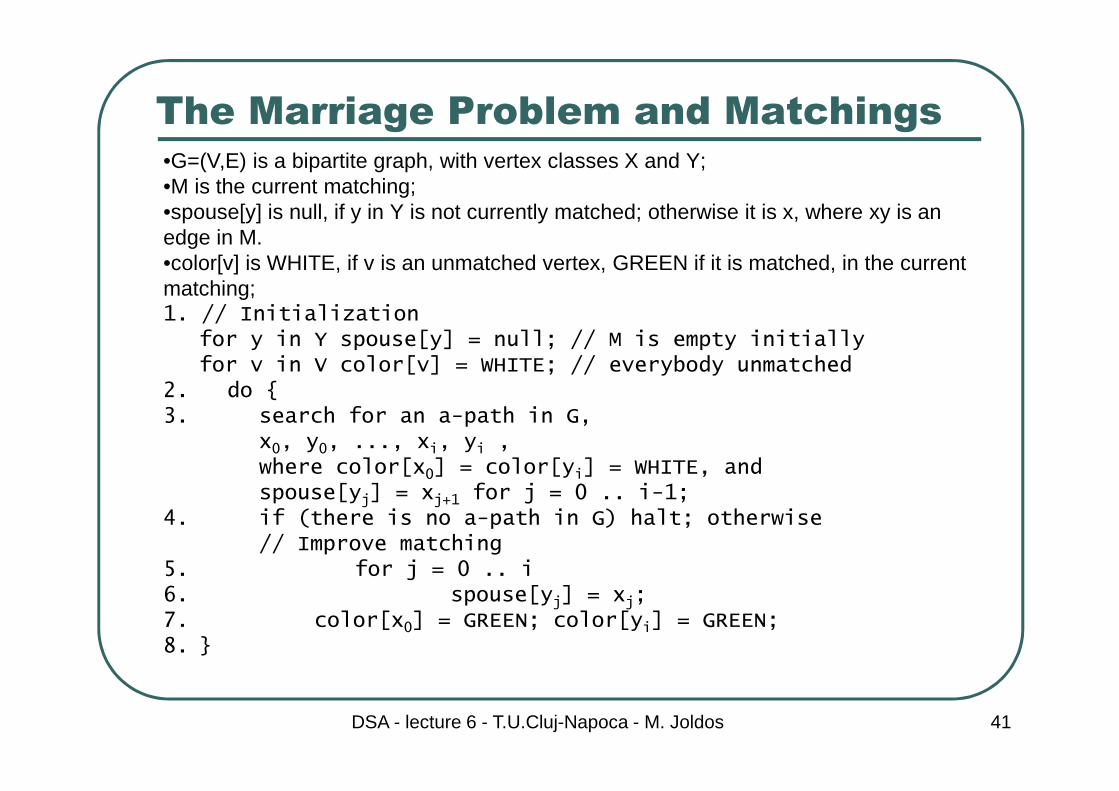
•G=(V,E) is a bipartite graph, with vertex classes X and Y; •M is the current matching; •spouse[y] is null, if y in Y is not currently matched; otherwise it is x, where xy is an edge in M. •color[v] is WHITE, if v is an unmatched vertex, GREEN if it is matched, in the current matching; 1. // Initialization
for y in Y spouse[y] = null; // M is empty initially for v in V color[v] = WHITE; // everybody unmatched
2. do { 3. search for an a-path in G,
x0, y0, ..., xi, yi , where color[x0] = color[yi] = WHITE, and spouse[yj] = xj+1 for j = 0 .. i-1;
4. if (there is no a-path in G) halt; otherwise // Improve matching
5. for j = 0 .. i6. spouse[yj] = xj; 7. color[x0] = GREEN; color[yi] = GREEN; 8. }

DSA - lecture 6 - T.U.Cluj-Napoca - M. Joldos 42
Reading
� AHU, chapter 7� Preiss, chapter: Graphs and Graph
Algorithms� CLR, chapter 23, section 2, chapter 24� CLRS chapter 22, section 2, 3, chapter 26
section 3� Notes