Embed Size (px)
Citation preview

Reservoir Engineering 2 Course (1st Ed.)
1. Introduction
2. Classification Of Aquifers
3. Recognition Of Natural Water Influx
1. Water Influx ModelsA. The Pot Aquifer Model
B. Schilthuis’ SS Model
C. Hurst’s Modified SS Model

Aquifer uncertainties
It should be appreciated that in reservoir engineering there are more uncertainties attached to this subject than to any other. This is simply because one seldom drills wells into
an aquifer to gain the necessary information about the porosity,
permeability, thickness, and fluid properties.
Instead, these properties frequently have to be inferred from what has been observed in the reservoir.
Even more uncertain, however, is the geometry and areal continuity of the aquifer itself.
Spring14 H. AlamiNia Reservoir Engineering 2 Course (1st Ed.) 5
Water influx model requirements
Several models have been developed for estimating water influx that are based on assumptions that describe
the characteristics of the aquifer.
Due to the inherent uncertainties in the aquifer characteristics, all of the proposed models require historical reservoir performance data
to evaluate constants representing aquifer property parameters since these are rarely known from exploration-development
drilling with sufficient accuracy for direct application.
Spring14 H. AlamiNia Reservoir Engineering 2 Course (1st Ed.) 6
evaluation of the constants
The material balance equation can be used to determine historical water influx provided original oil in place is known from pore volume estimates.
This permits evaluation of the constants in the influx equations so that future water influx rate can be forecasted.
Spring14 H. AlamiNia Reservoir Engineering 2 Course (1st Ed.) 7
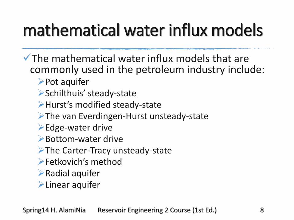
mathematical water influx models
The mathematical water influx models that are commonly used in the petroleum industry include:Pot aquiferSchilthuis’ steady-stateHurst’s modified steady-stateThe van Everdingen-Hurst unsteady-stateEdge-water driveBottom-water driveThe Carter-Tracy unsteady-stateFetkovich’s methodRadial aquiferLinear aquifer
Spring14 H. AlamiNia Reservoir Engineering 2 Course (1st Ed.) 8
The Pot Aquifer Model; Basis
The simplest model that can be used to estimate the water influx into a gas or oil reservoir is based on the basic definition of compressibility.
A drop in the reservoir pressure, due to the production of fluids, causes the aquifer water to expand and flow into the reservoir.
The compressibility is defined mathematically as:
ΔV = c V Δ p
Spring14 H. AlamiNia Reservoir Engineering 2 Course (1st Ed.) 10

The Pot Aquifer Model; all directions water encroachmentApplying the above basic compressibility definition
to the aquifer gives:
Water influx = (aquifer compressibility) *(initial volume of water) * (pressure drop) or
We = cumulative water influx, bblcw = aquifer water compressibility, psi−1cf = aquifer rock compressibility, psi−1Wi = initial volume of water in the aquifer, bblpi = initial reservoir pressure, psip = current reservoir pressure
(pressure at oil-water contact), psi
Spring14 H. AlamiNia Reservoir Engineering 2 Course (1st Ed.) 11

The Pot Aquifer Model; initial volume of waterCalculating the initial volume of water
in the aquifer requires the knowledge of aquifer dimension and properties. These, however,
are seldom measured since wells are not deliberately drilled into the aquifer to obtain such information.
For instance, if the aquifer shape is radial, then:ra = radius of the aquifer, ft
re = radius of the reservoir, ft
h = thickness of the aquifer, ft
φ = porosity of the aquifer
Spring14 H. AlamiNia Reservoir Engineering 2 Course (1st Ed.) 12
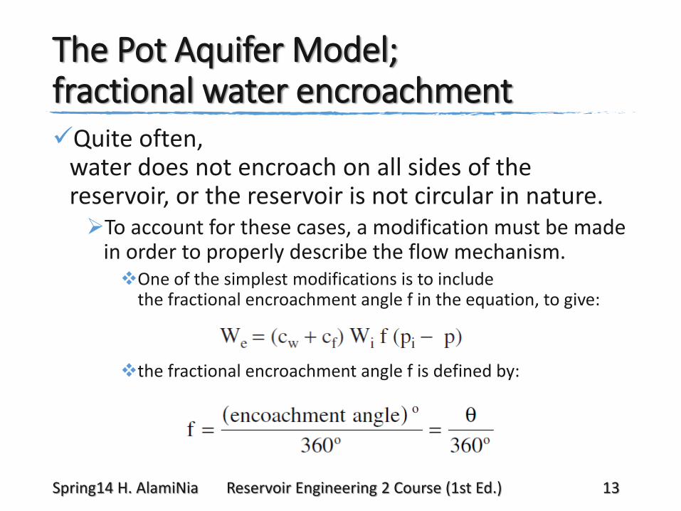
The Pot Aquifer Model; fractional water encroachmentQuite often,
water does not encroach on all sides of the reservoir, or the reservoir is not circular in nature. To account for these cases, a modification must be made
in order to properly describe the flow mechanism. One of the simplest modifications is to include
the fractional encroachment angle f in the equation, to give:
the fractional encroachment angle f is defined by:
Spring14 H. AlamiNia Reservoir Engineering 2 Course (1st Ed.) 13
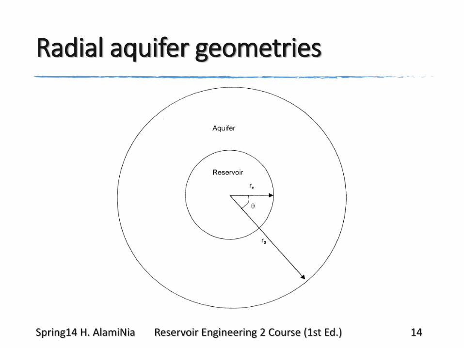
Radial aquifer geometries
Spring14 H. AlamiNia Reservoir Engineering 2 Course (1st Ed.) 14

Dake consideration
The Pot Aquifer Model is only applicable to a small aquifer, i.e., pot aquifer, whose dimensions
are of the same order of magnitude as the reservoir itself.
Dake (1978) points out that because the aquifer is considered relatively small, a pressure drop in the reservoir is instantaneously transmitted
throughout the entire reservoir-aquifer system.
Dake suggests that for large aquifers, a mathematical model is required which includes
time dependence to account for the fact that it takes a finite time for the aquifer to respond to a pressure change in the reservoir.
Spring14 H. AlamiNia Reservoir Engineering 2 Course (1st Ed.) 15

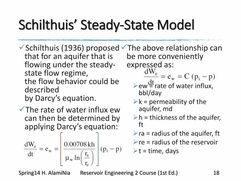
Schilthuis’ Steady-State Model
Schilthuis (1936) proposed that for an aquifer that is flowing under the steady-state flow regime, the flow behavior could be described by Darcy’s equation.
The rate of water influx ew can then be determined by applying Darcy’s equation:
The above relationship can be more conveniently expressed as:
ew = rate of water influx, bbl/day
k = permeability of the aquifer, md
h = thickness of the aquifer, ft
ra = radius of the aquifer, ftre = radius of the reservoirt = time, days
Spring14 H. AlamiNia Reservoir Engineering 2 Course (1st Ed.) 18

Schilthuis’ Steady-State Model; Influx constantThe parameter C is called the water influx constant
and is expressed in bbl/day/psi. This water influx constant C may be calculated
from the reservoir historical production data over a number of selected time intervals, provided that the rate of water influx ew has been determined independently from a different expression. For instance, the parameter C may be estimated by combining
the Equation with ew = Qo Bo + Qg Bg + Qw Bw.
Although the influx constant can only be obtained in this manner when the reservoir pressure stabilizes, once it has been found, it may be applied to both stabilized and changing reservoir pressures.
Spring14 H. AlamiNia Reservoir Engineering 2 Course (1st Ed.) 19
Notes
If the steady-state approximation adequately describes the aquifer flow regime, the calculated water influx constant C values
will be constant over the historical period.
Note that the pressure drops contributing to influx are the cumulative pressure drops from the initial pressure.
Spring14 H. AlamiNia Reservoir Engineering 2 Course (1st Ed.) 20
the cumulative water influx
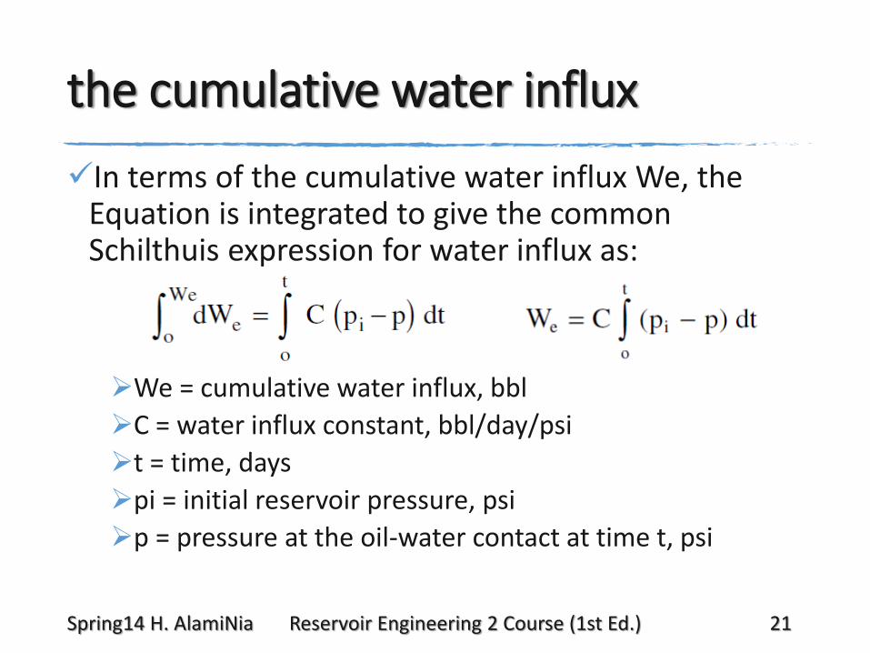
In terms of the cumulative water influx We, the Equation is integrated to give the common Schilthuis expression for water influx as:
We = cumulative water influx, bbl
C = water influx constant, bbl/day/psi
t = time, days
pi = initial reservoir pressure, psi
p = pressure at the oil-water contact at time t, psi
Spring14 H. AlamiNia Reservoir Engineering 2 Course (1st Ed.) 21
Calculating the area under the curve
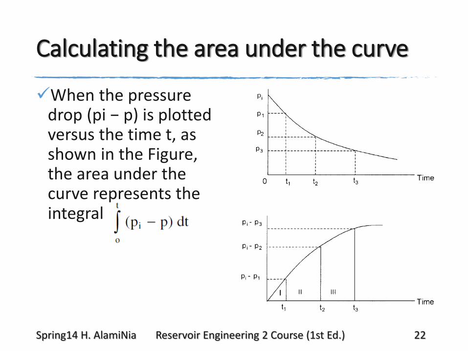
When the pressure drop (pi − p) is plotted versus the time t, as shown in the Figure, the area under the curve represents the integral
Spring14 H. AlamiNia Reservoir Engineering 2 Course (1st Ed.) 22
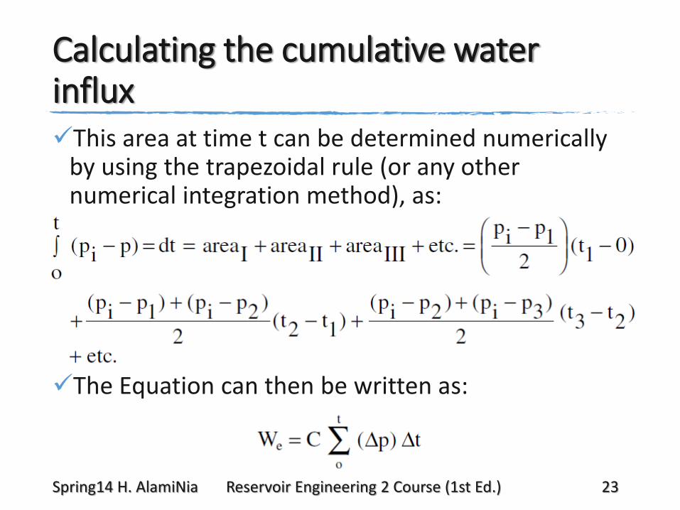
Calculating the cumulative water influxThis area at time t can be determined numerically
by using the trapezoidal rule (or any other numerical integration method), as:
The Equation can then be written as:
Spring14 H. AlamiNia Reservoir Engineering 2 Course (1st Ed.) 23
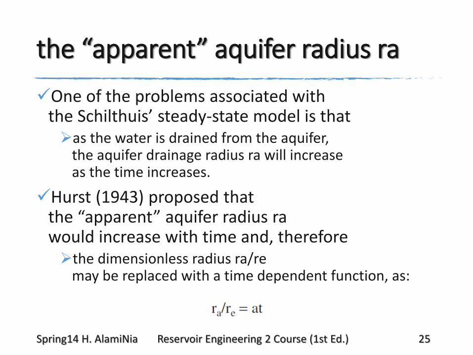
the “apparent” aquifer radius ra
One of the problems associated with the Schilthuis’ steady-state model is that as the water is drained from the aquifer,
the aquifer drainage radius ra will increase as the time increases.
Hurst (1943) proposed that the “apparent” aquifer radius ra would increase with time and, therefore the dimensionless radius ra/re
may be replaced with a time dependent function, as:
Spring14 H. AlamiNia Reservoir Engineering 2 Course (1st Ed.) 25
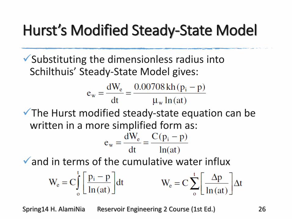
Hurst’s Modified Steady-State Model
Substituting the dimensionless radius into Schilthuis’ Steady-State Model gives:
The Hurst modified steady-state equation can be written in a more simplified form as:
and in terms of the cumulative water influx
Spring14 H. AlamiNia Reservoir Engineering 2 Course (1st Ed.) 26
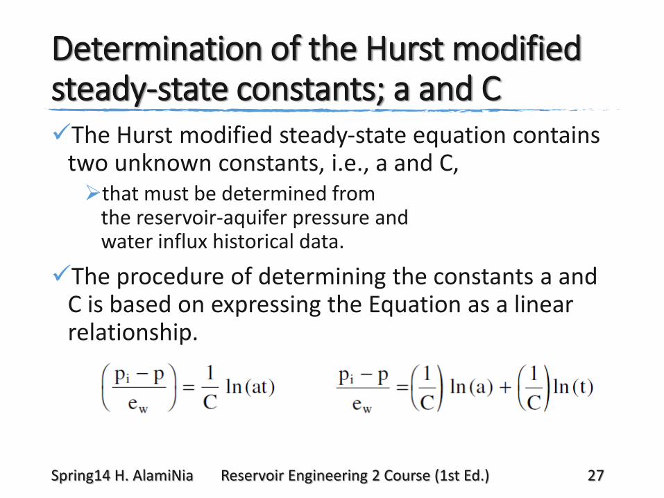
Determination of the Hurst modified steady-state constants; a and CThe Hurst modified steady-state equation contains
two unknown constants, i.e., a and C, that must be determined from
the reservoir-aquifer pressure and water influx historical data.
The procedure of determining the constants a and C is based on expressing the Equation as a linear relationship.
Spring14 H. AlamiNia Reservoir Engineering 2 Course (1st Ed.) 27
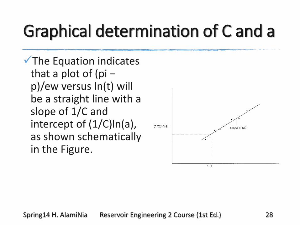
Graphical determination of C and a
The Equation indicates that a plot of (pi − p)/ew versus ln(t) will be a straight line with a slope of 1/C and intercept of (1/C)ln(a), as shown schematically in the Figure.
Spring14 H. AlamiNia Reservoir Engineering 2 Course (1st Ed.) 28
1. Ahmed, T. (2010). Reservoir engineering handbook (Gulf Professional Publishing). Chapter 10

1. mathematical Water Influx models;A. The van Everdingen-Hurst Unsteady-State Model
a. Edge-Water DriveI. computational steps for We at successive intervals