. RESEARCH PAPER .Special Focus

SCIENCE CHINAInformation Sciences

May 2012 Vol. 55 No. 5: 983–993

doi: 10.1007/s11432-012-4574-y

c© Science China Press and Springer-Verlag Berlin Heidelberg 2012 info.scichina.com www.springerlink.com

Lp shape deformation

GAO Lin1∗, ZHANG GuoXin1 & LAI YuKun2

1Department of Computer Science and Technology, Tsinghua University, Beijing 100084, China;2School of Computer Science and Informatics, Cardiff University, Wales CF24 3AA, UK

Received October 24, 2011; accepted January 6, 2012; published online March 16, 2012

Abstract Shape deformation is a fundamental tool in geometric modeling. Existing methods consider pre-

serving local details by minimizing some energy functional measuring local distortions in the L2 norm. This

strategy distributes distortions quite uniformly to all the vertices and penalizes outliers. However, there is no

unique answer for a natural deformation as it depends on the nature of the objects. Inspired by recent sparse

signal reconstruction work with non L2 norm, we introduce general Lp norms to shape deformation; the positive

parameter p provides the user with a flexible control over the distribution of unavoidable distortions. Compared

with the traditional L2 norm, using smaller p, distortions tend to be distributed to a sparse set of vertices,

typically in feature regions, thus making most areas less distorted and structures better preserved. On the

other hand, using larger p tends to distribute distortions more evenly across the whole model. This flexibility is

often desirable as it mimics objects made up with different materials. By specifying varying p over the shape,

more flexible control can be achieved. We demonstrate the effectiveness of the proposed algorithm with various

examples.

Keywords shape deformation, Lp norm, geometric modeling

Citation Gao L, Zhang G X, Lai Y K. Lp shape deformation. Sci China Inf Sci, 2012, 55: 983–993, doi:

10.1007/s11432-012-4574-y

1 Introduction

The proliferation of digital geometry models nowadays makes digitized 3D objects, often representedas triangulated meshes, widely available. In addition to direct capture 3D shapes from real objects, avariety of geometric modeling tools have been developed. Surface deformation is a fundamental tool thatproduces altered shapes effectively. This has various applications including editing shapes to suit theneeds, producing sequences of objects for animation and simulating the deformation of objects in VRsystems [1] such as virtual surgery simulation systems [2]. Shape deformation has received a lot of at-tention in recent years. Since physically modeling geometric objects undergoing deformation is bothdifficult and computationally expensive, most algorithms focus on using geometric shape informationalone. There is no single “correct” answer for surface deformation, due to the potential variable mate-rial natures. Many existing methods produce deformed objects by minimizing some energy functionalmeasuring the usually unavoidable distortions incurred in the deformation process. To support general,large-scale deformation, energies need to be defined locally, as these properties tend to be well preserved∗Corresponding author (email: gaolinorange@gmail.com)

984 Gao L, et al. Sci China Inf Sci May 2012 Vol. 55 No. 5

after deformation. The L2 norm is often used to combine local energies, often defined at some element(e.g. vertex) level. This strategy tends to spread out unavoidable distortions to all the vertices quiteuniformly and penalize outliers. Although working reasonably well for a large set of models, this maynot lead to the most “natural” deformation in practice. Distributions of unavoidable distortions reflectthe material nature and the design intentions of the user, thus giving the user intuitive control is oftendesirable. In this work, inspired by recent advances in sparse signal reconstruction [3,4] and surfacereconstruction [5], we introduce Lp norms for surface deformation instead of the traditional L2 norm,in the energy functional combining local energies. More precisely, assuming the local energy associatedwith the ith element (e.g. vertex) is Ei, the overall energy E is defined in a more general manner asE =

∑i wi‖Ei‖p, where p is a positive parameter to flexibly control the distributions of unavoidable

distortions after the deformation. For practical use, we assume p � 1. p = 2 leads to the traditionalL2 norm. Using smaller p tends to distribute unavoidable distortions to a sparse set of vertices, often infeature regions. A typical case is p = 1 which reduces to the L1 norm used in sparse shape reconstruction[5]. A brief theoretical explanation of the sparsity when p = 1 is given in Appendix. This has some nicefeatures such as making most areas less distorted and structures better preserved. Using larger p tendsto distribute distortions more evenly as outliers are more significantly penalized. Using our approach, awide range of deformation results can be obtained, which gives the user effective and intuitive controlover the deformation process. Results obtained with different p’s may all be natural, mimicking objectsmade up with different materials. Our implementation is based on [6], which optimizes an energy func-tional for locally as-rigid-as-possible deformation. The idea could be used in other surface deformationframework as well. We show that using our Lp norm, the energy functional is convex and thus can beeffectively optimized to the global minimum with iterative backtracking line search [7]. In Section 2, wereview the most relevant work. The algorithm is described in detail in Section 3. Experimental resultsand discussions are presented in Section 4 and finally concluding remarks and future work are given inSection 5.

2 Related work

Shape deformation is an active research direction in recent decades. A large amount of research work hasbeen carried out in the field. A complete survey is beyond the scope of this paper. Please refer to [8–10]for recent surveys of surface deformation techniques. Here we only review the most relevant work to thisresearch.

The key principle of surface deformation algorithms is to produce visually plausible deformation andfollow the deformation of actual physical objects. Surface based deformation can be modeled as an energyminimization problem with boundary constraints from user input (such as handle movements or specifiedlocal frames at certain positions). A natural approach is to deform the model according to the physicalrules [11–13]. These physically based methods involve solving partial differential equations which arecomplicated and time consuming to achieve accurate deformation results. To improve the computationalefficiency, Barbic et al. [14] proposed a large-scale deformation method by decomposing the deformableobject into components.

Skeletons are used to deform the images/videos (e.g. [15]) and surface models [16–19]. These skeletondriven deformation methods need extra efforts to construct skeletons. Some works deform the shapeby building the coarse cages encompassing the shape [20–24]. Such deformations may also be achievedcage-free, as demonstrated in [25] by using umbrella shaped cells constructed automatically. A newapproach [26] has been proposed recently which allows the user to freely combine different types ofhandles to deform the object.

Another strategy to make intuitive deformation results is to preserve details and/or volumes afterdeformation. Local differential coordinate are used to encode local details and recover them after defor-mation. These methods include rotation invariant coordinate for better handling rotations [27], Laplaciancoordinates [28], Poisson-based gradient field [29], and iterative dual Laplacian approach for improvedresults [30]. Volumetric Laplacian constructed in the interior of the shape is proposed to better preserve

Gao L, et al. Sci China Inf Sci May 2012 Vol. 55 No. 5 985

the volume [31,32]. A subspace technique is used for efficiently optimizing the nonlinear energy first atthe coarser mesh and uses 3D mean value coordinates [20] for interpolation on the original mesh.

Rigidity is an important principle in deformation that is well studied. Terzopoulos et al. [11] formulatea shell energy to measure the distortions between the input and the deformed models.

E(S, S′) =∫

Ω

(ks‖I − I ′‖2 + kb‖II − II ′‖2)dudv, (1)

where S and S′ are the surfaces before and after deformation, I, II are the first and second fundamentalforms before deformation, and I ′, II ′ are corresponding fundamental forms after deformation; they areused to measure the shearing and bending incurred by the deformation. ks and kb are two coefficients tobalance the terms. The energy E(S, S′) reaches zero only for completely rigid transformations. Practicalsolutions often involve unavoidable distortions, and thus only achieves the minimizer of E. Preservinglocal as-rigid-as-possible is practically useful as this preserves geometric shape and features while allowingfor sufficient flexibility for deformation. Sorkine et al. [6] estimate the rigid transformations of local cellsand collect the transformations to deform the whole model. The principle of as rigid as possible defor-mation has also been applied to shape interpolation [33] and shape manipulation [34]. Such works basedon the as-rigid-as-possible principle have a similar framework. They all estimate local rigid transforms ofgeometric elements (e.g. triangle faces), and then build a global energy formulation based on L2 norm.L1 norm was recently used to reconstruct point set surfaces, and has achieved sparse optimization withimproved feature and structure preservation [5]. Bougleux et al. [35] recently used similar formulation inp-Laplacian, and applied this for applications such as mesh denoising.

Differential domain methods and local as-rigid-as-possible methods mentioned above are mainly con-cerned with surface deformation with uniform material properties. Some previous works consider non-uniform materials. Popa et al. [36] use a painting-like interface to specify the material properties, whichare then used to guide the propagation of transformations. Our method does not need user interactionsto specify material properties. Instead we use a single parameter to control the distribution of deforma-tion distortions. Thus our approach provides more flexibility than most traditional deformation methodswhile having less burden on user efforts. Some research work explicitly considers man-made models. Theyare often self-similar and made up of piecewise quasi-rigid components. Gal et al. [37] extract featurecurves according to the analysis of the models and manipulate the models through editing these curves.In this paper, we introduce general Lp norm in the energy formulation for surface deformation, leadingto flexible and intuitive control of residual error distributions.

3 Algorithm

In this section, we first describe our Lp surface deformation formulation in the as-rigid-as-possible frame-work. We then show that the resulting energy functional is convex, leading to an effective optimizationalgorithm.

3.1 Lp surface deformation formulation

We denote the input triangle mesh by S which contains n vertices. For each vertex vi, one-ring neighborsform a set, denoted by Ni. We use pi ∈ R

3 to represent the position of vi. The surface is deformed intoS′ with the same connectivity and positions changed to p′i. To define local rigidity, similar to [6], for eachvertex vi, a cell Ci is formed which covers 1-ring neighbors Ni. This definition is sufficiently local andinvolves overlaps between cells which are essential for smoothness of transforms between cells. The localenergy between the cell Ci and its deformation C′

i is defined similarly to [6]

E(Ci, C′i) =

√ ∑

j∈Ni

wij‖(p′i − p′j) − Ri(pi − pj)‖2. (2)

Here, Ri represents a 3 × 3 rotation matrix that transforms locally from Ci to C′i. The weight wij can

be chosen as the cotangent weight wij = 12 (cotαij + cotβij) [38] to take mesh discretization into account,

986 Gao L, et al. Sci China Inf Sci May 2012 Vol. 55 No. 5

where αij and βij are angles opposite to the edge vivj . To form the overall energy, we propose to use Lp

norm instead of the traditional L2 norm:

E(S, S′) =n∑

i=1

E(Ci, C′i)

p =n∑

i=1

{ ∑

j∈Ni

wij‖(p′i − p′j) − Ri(pi − pj)‖2

} p2

. (3)

To minimize the nonlinear energy E(S, S′), an iterative algorithm is used. From an initial guess whichcan take either the input mesh or the mesh obtained from relatively simple deformation algorithms,rotation matrices Ri and positions p′i are optimized in turn. This process guarantees convergence as theenergy is monotonically decreasing. The optimal rotation matrix Ri for fixed positions p′i can be solvedindependently for each vertex vi [5]. Denote by Si the covariance matrix of Ci. Si =

∑j∈Ni

wij(pi −pj)(p′i − p′j)

T. Singular decomposition of Si satisfies Si = UiΣiVTi , and then Ri can be obtained as

Ri = ViUTi , subject to changing the sign of the column of Ui corresponding to the minimal singular

value, to make det(Ri) > 0. We will give the details of finding the optimal positions p′i for given Ri inthe next subsection.

3.2 An effective convex optimization

To find the optimal positions p′i, we first prove that the energy E w.r.t. p′i is convex. The position pi ateach vertex vi is three dimensional, and denoted by pix, piy, piz. We take P to represent a vector collectingall of these coordinates, i.e. P = [p1x, p1y, p1z, . . . , pnx, pny, pnz]T. Since Ri’s are fixed. Ri(pi − pj) isconstant vector which can be expressed as the difference of two vectors.

Eq. (2) can be rewritten as

E(Ci, C′i) =

√ ∑

j∈Ni

wij‖aTij(P − d)‖2, (4)

E(Ci, C′i) =

√√√√(P − d)T

( ∑

j∈Ni

w2ija

Tijaij

)

(P − d), (5)

where aij is a vector of length 3n. aij(k) = 1, for k = 3i − 2, 3i − 1, 3i and aij(k) = −1, for k =3j − 2, 3j − 1, 3j. For any other k, aij(k) = 0. aT

ijd = Ri(pi − pj). To show that the energy definedin Eq. (3) is convex, since

∑j∈Ni

w2ija

Tijaij is symmetric semi-positive definite, it suffices to prove that

this holds for a more generalized function, namely for a symmetric semi-positive definite matrix A, andp � 1, c � 0, the form f = (xTAx + c)

p2 is convex. The gradient ∇f and Hessian matrix H(f) of f can

be calculated as

∇f = p(Ax)(xTAx + c)p−22 , (6)

H(f) = p(xTAx + c)p−42 · [A(xTAx + c) + (p − 2)AxxTA]. (7)

As p � 1, it suffices to show that for a general vector y,

(yTAy)(xTAx) � (yTAxxTAy) = (yTAx)2. (8)

Since A is symmetric semi-positive definite, there exists a unique symmetric semi-positive definite matrixB, such that B · B = A. We use

√A to represent the matrix B, which can be calculated using eigen

decomposition. In this case, Eq. (8) actually holds due to the following inequality

[(√

Ay)T(√

Ay)][(√

Ax)T(√

Ax)] � [(√

Ay)T(√

Ax)]2. (9)

If c = 0, the Hessian matrix H(f) may not exist when Ax = 0. This situation can be verified byshowing that f is convex when restricted to any line. More specifically, assume f = g(t), t ∈ R, then∃t, g(t) = 0 if and only if g(t) ≡ 0, so either g′′ exists for every t, or g(t) ≡ 0. In both cases, our conclusionis proved.

Gao L, et al. Sci China Inf Sci May 2012 Vol. 55 No. 5 987

Since the energy is convex, we can find the global minimum effectively by an iterative backtrackingline search [7]. Starting from p′i, we compute the descent direction

Δp′i = −∂E

∂p′i

∣∣∣∣p

′i = p′i, (10)

as the negative gradient direction. Assume all the p′i form p′ and all the Δp′i form Δp′. The step size t

is initialized to 1 and can be obtained by repeatedly multiplying t by a constant β, until E(p′ + tΔp′) �E(p′) + αt∇E(p′)TΔp′. We choose α = 0.3 and β = 0.5 for our experiments. The updated position canthen be obtained as p′ + tΔp′. This process repeats until convergence happens.

3.3 More efficient solution of the L1 problem

Using L1 norm (the special case with p = 1) has a few advantages. The distortions tend to concentrateon a sparse set of vertices, leading to generally well preserved shapes after deformation. The problem canbe converted to the dual form of conic programming as follows. Based on Eq. (3), we introduce variablesT1, T2, . . . , Tn, and these variables along with optimized positions p′i are unknown variables to optimize.We need to maximize

∑ni=1(−Ti), subject to the constraints

Ti �√ ∑

j∈Ni

‖√wij((p′i − p′j) − Ri(pi − pj))‖2. (11)

This can be effectively solved using SDPT3 (an open source conic programming solver) [39].

4 Experimental results

We carried out our experiments on a desktop computer with 2× Quad 2.27 GHz CPUs. Our currentimplementation has not been optimized for multi-core CPUs. In all the examples, we use blue dotsto indicate the handles used to control the deformation, and use color coding to show the distortiondistributions incurred by the deformation (E(Ci, C

′i) for each vertex vi), where increasing distortions are

represented using colors from blue to red. We use conic programming described in Subsection 3.3 tosolve L1 problem, the method in [6] to solve L2 problem and backtracking line search described in 3.2to solve other Lp problems. For all the examples, we initialize the deformed mesh with naive Laplaciandeformation (as in [28] without rotation estimation). Assuming for each vertex vi the position change

after each iteration is Δpi, the average displacement is defined as d =√∑

ni=1 ‖Δpi‖2

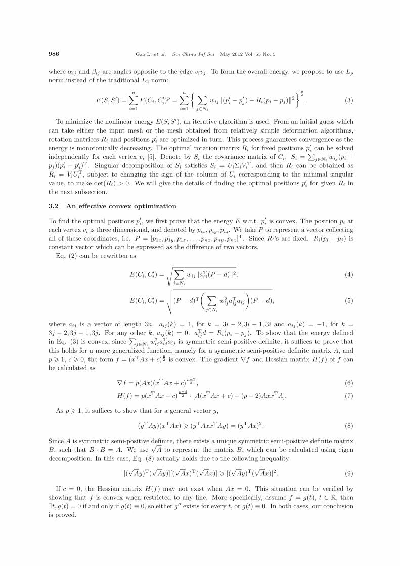
n . The terminatingcondition of convergence is indicated by d < εC (for conic programming) and d < εL (for line search)respectively. Different thresholds are used because these two optimization methods tend to update thepositions differently. We have found εC = 0.01 and εL = 0.00005 work well in practice and these sameparameters are used for all the examples in the paper. Detailed statistics of iteration numbers and runningtimes are given in Table 1.

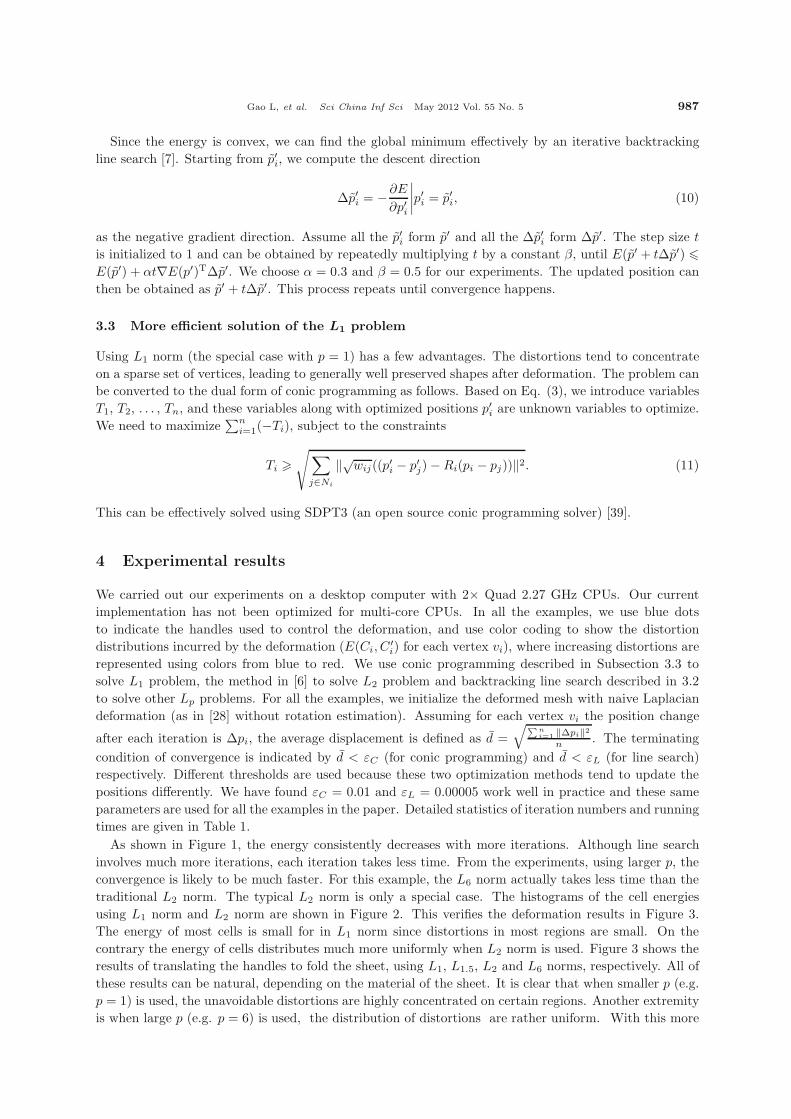
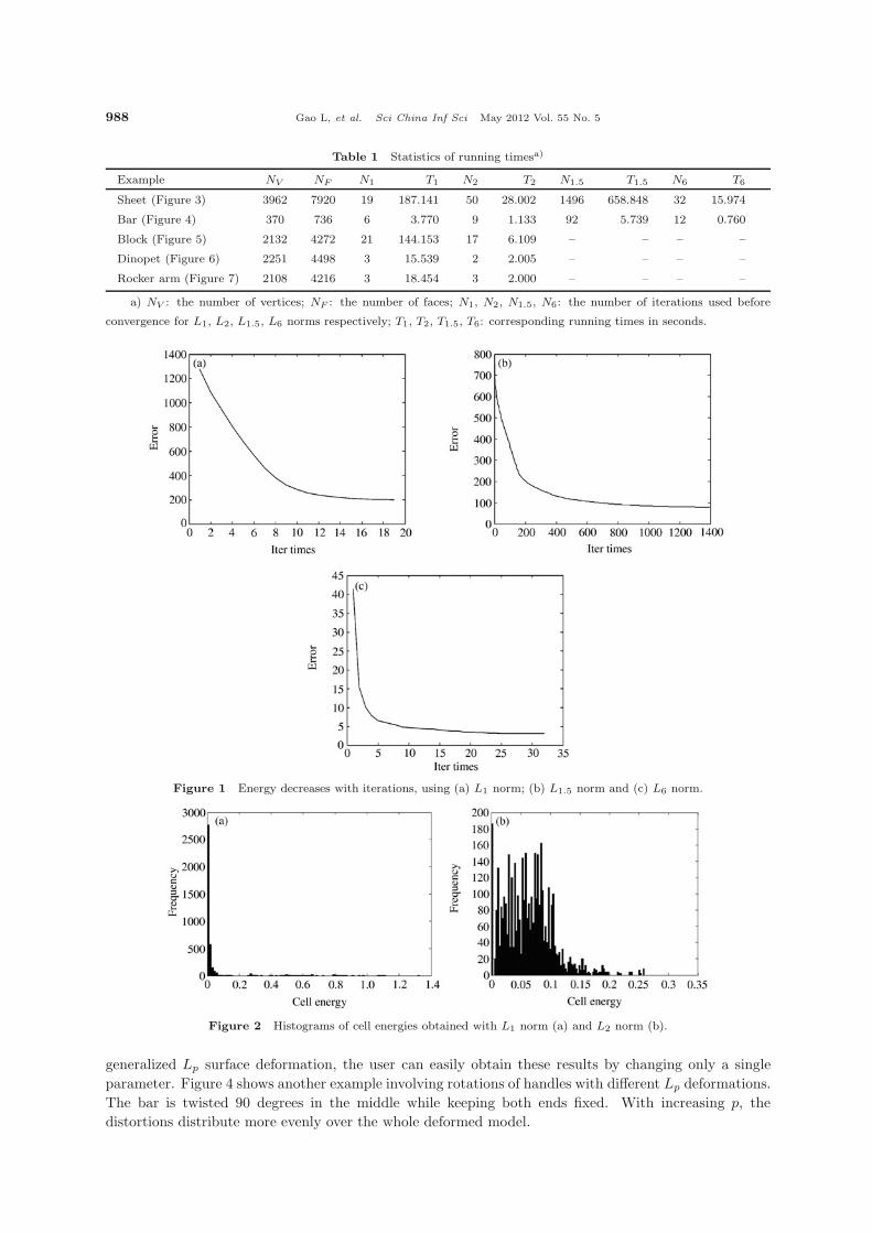
As shown in Figure 1, the energy consistently decreases with more iterations. Although line searchinvolves much more iterations, each iteration takes less time. From the experiments, using larger p, theconvergence is likely to be much faster. For this example, the L6 norm actually takes less time than thetraditional L2 norm. The typical L2 norm is only a special case. The histograms of the cell energiesusing L1 norm and L2 norm are shown in Figure 2. This verifies the deformation results in Figure 3.The energy of most cells is small for in L1 norm since distortions in most regions are small. On thecontrary the energy of cells distributes much more uniformly when L2 norm is used. Figure 3 shows theresults of translating the handles to fold the sheet, using L1, L1.5, L2 and L6 norms, respectively. All ofthese results can be natural, depending on the material of the sheet. It is clear that when smaller p (e.g.p = 1) is used, the unavoidable distortions are highly concentrated on certain regions. Another extremityis when large p (e.g. p = 6) is used, the distribution of distortions are rather uniform. With this more

988 Gao L, et al. Sci China Inf Sci May 2012 Vol. 55 No. 5

Table 1 Statistics of running timesa)

Example NV NF N1 T1 N2 T2 N1.5 T1.5 N6 T6

Sheet (Figure 3) 3962 7920 19 187.141 50 28.002 1496 658.848 32 15.974

Bar (Figure 4) 370 736 6 3.770 9 1.133 92 5.739 12 0.760

Block (Figure 5) 2132 4272 21 144.153 17 6.109 – – – –

Dinopet (Figure 6) 2251 4498 3 15.539 2 2.005 – – – –

Rocker arm (Figure 7) 2108 4216 3 18.454 3 2.000 – – – –

a) NV : the number of vertices; NF : the number of faces; N1, N2, N1.5, N6: the number of iterations used before

convergence for L1, L2, L1.5, L6 norms respectively; T1, T2, T1.5, T6: corresponding running times in seconds.

Figure 1 Energy decreases with iterations, using (a) L1 norm; (b) L1.5 norm and (c) L6 norm.

Figure 2 Histograms of cell energies obtained with L1 norm (a) and L2 norm (b).

generalized Lp surface deformation, the user can easily obtain these results by changing only a singleparameter. Figure 4 shows another example involving rotations of handles with different Lp deformations.The bar is twisted 90 degrees in the middle while keeping both ends fixed. With increasing p, thedistortions distribute more evenly over the whole deformed model.

Gao L, et al. Sci China Inf Sci May 2012 Vol. 55 No. 5 989

(a) (b) (c) (d) (e) (f) (g) (h) (i)

Figure 3 Results of Lp surface deformations. (a) The input surface; (b)(d)(f)(h) the results with L1, L1.5, L2 and L6

norms respectively; (c)(e)(g)(i) color coded distortion distributions of (b)(d)(f)(h). Distortions increase from blue to red.

(a) (b) (c) (d) (e) (f) (g) (h) (i)

Figure 4 Results of Lp surface deformations. (a) The input surface; (b)(d)(f)(h) the results with L1, L1.5, L2 and L6

norms respectively; (c)(e)(g)(i) color coded distortion distributions of (b)(d)(f)(h). Distortions increase from blue to red.

(a) (b) (c) (d) (e)

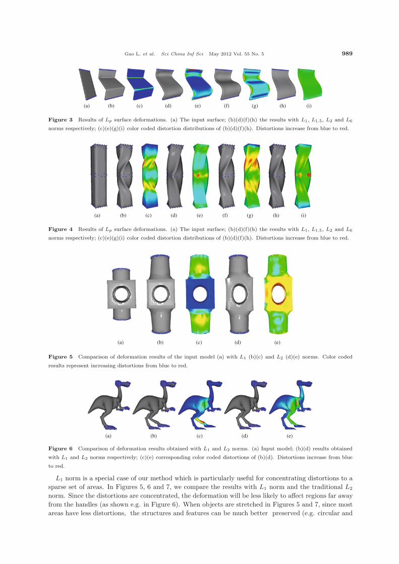
Figure 5 Comparison of deformation results of the input model (a) with L1 (b)(c) and L2 (d)(e) norms. Color coded

results represent increasing distortions from blue to red.

(a) (b) (c) (d) (e)

Figure 6 Comparison of deformation results obtained with L1 and L2 norms. (a) Input model; (b)(d) results obtained

with L1 and L2 norms respectively; (c)(e) corresponding color coded distortions of (b)(d). Distortions increase from blue

to red.

L1 norm is a special case of our method which is particularly useful for concentrating distortions to asparse set of areas. In Figures 5, 6 and 7, we compare the results with L1 norm and the traditional L2

norm. Since the distortions are concentrated, the deformation will be less likely to affect regions far awayfrom the handles (as shown e.g. in Figure 6). When objects are stretched in Figures 5 and 7, since mostareas have less distortions, the structures and features can be much better preserved (e.g. circular and

990 Gao L, et al. Sci China Inf Sci May 2012 Vol. 55 No. 5

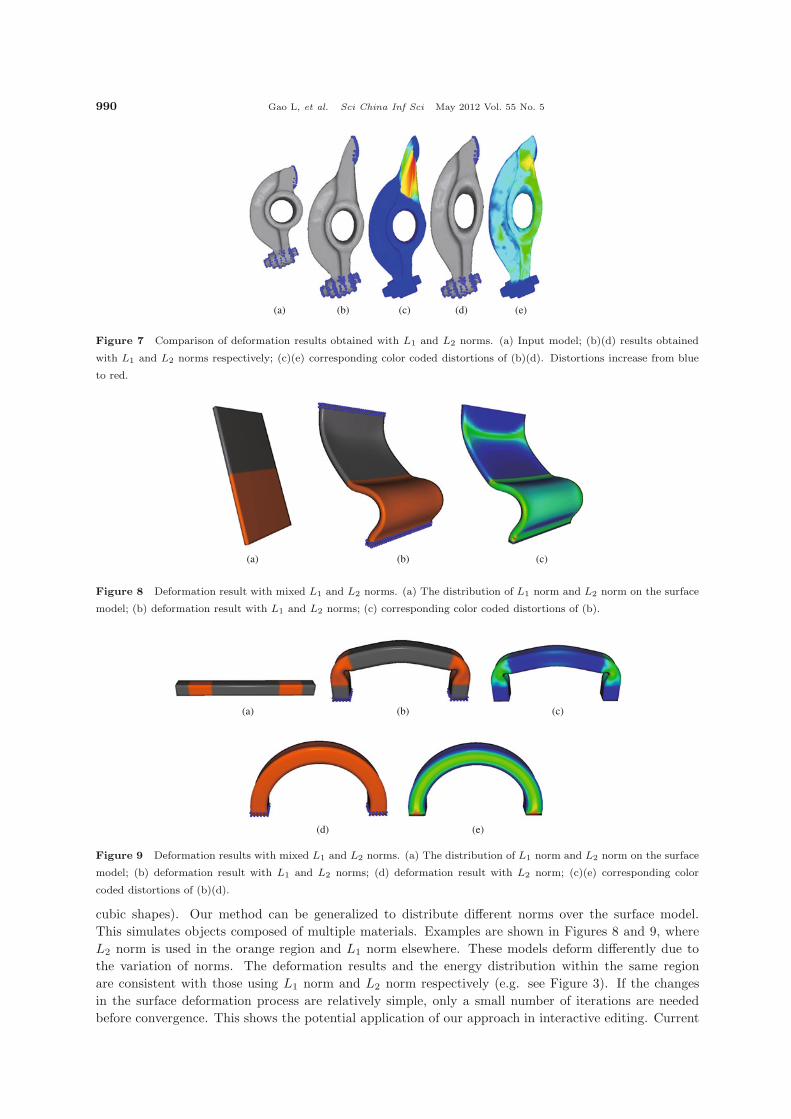
(a) (b) (c) (d) (e)

Figure 7 Comparison of deformation results obtained with L1 and L2 norms. (a) Input model; (b)(d) results obtained

with L1 and L2 norms respectively; (c)(e) corresponding color coded distortions of (b)(d). Distortions increase from blue

to red.

(a) (b) (c)

Figure 8 Deformation result with mixed L1 and L2 norms. (a) The distribution of L1 norm and L2 norm on the surface

model; (b) deformation result with L1 and L2 norms; (c) corresponding color coded distortions of (b).

(a) (b) (c)

(d) (e)

Figure 9 Deformation results with mixed L1 and L2 norms. (a) The distribution of L1 norm and L2 norm on the surface

model; (b) deformation result with L1 and L2 norms; (d) deformation result with L2 norm; (c)(e) corresponding color

coded distortions of (b)(d).

cubic shapes). Our method can be generalized to distribute different norms over the surface model.This simulates objects composed of multiple materials. Examples are shown in Figures 8 and 9, whereL2 norm is used in the orange region and L1 norm elsewhere. These models deform differently due tothe variation of norms. The deformation results and the energy distribution within the same regionare consistent with those using L1 norm and L2 norm respectively (e.g. see Figure 3). If the changesin the surface deformation process are relatively simple, only a small number of iterations are neededbefore convergence. This shows the potential application of our approach in interactive editing. Current

Gao L, et al. Sci China Inf Sci May 2012 Vol. 55 No. 5 991

unoptimized implementation takes under 20 seconds (for ‘dinopet’ for example). We expect to explorepotential speed-up in the future, as detailed in the next section.

5 Conclusions and future work

In this paper, we propose a novel surface deformation approach that optimizes energy functional basedon general Lp norms. The extra parameter p provides the user with intuitive and flexible control overthe deformation process. Continuous variations of results can be obtained by simply changing a singleparameter. We have demonstrated that the effects of different p’s can be well anticipated. Using smallerp (e.g. L1 norm) makes distortions well concentrated on a sparse set of vertices, producing results withmost areas less distorted and structures better preserved. Larger p on the other hand promotes evendistribution of distortions. This flexibility mimics deforming objects with different material natures. Amajor limitation is that our method is relatively slow, due to its nonlinear nature. We would like toexplore potential techniques to speed up the computation, including subspace technique and parallelism.The optimization currently used such as iterative line search can be well parallelized using either multi-core CPUs or the GPU, which can potentially improve the performance quite significantly. With suchfurther development, interactive performance is possible to achieve as fewer iterations are often neededfor relatively small changes in interactive editing. In our current approach, we assign different normsmanually to simulate different material properties. In certain cases, where material stiffness is related togeometric properties (for example, joints are more flexible than rigid components), it is possible to developan automatic algorithm to distribute norms over the surface based on the geometry. This approach canalso be extended to other techniques such as content-aware model resizing [40]. Using the Lp norm inshape deformation is general to be incorporated in other shape deformation frameworks; we expect toexplore this in the future.

Acknowledgements

This work was supported by National Basic Research Project of China (Grant No. 2011CB302203), Natural

Science Foundation of China (Grant No. 61120106007). The third author is supported by Engineering and

Physical Sciences Research Council (Grant No. EP/I000100/1).

References

1 Bottcher G, Allerkamp D, Wolter F E. Multi-rate coupling of physical simulations for haptic interaction with de-

formable objects. Vis Comput, 2010, 26: 903–914

2 Chang J, Yang X S, Pan J J, et al. A fast hybrid computation model for rectum deformation. Vis Comput, 2011, 27:

97–107

3 Candes E J, Romberg J, Tao T. Robust uncertainty principles: exact signal reconstruction from highly incomplete

frequency information. IEEE Trans Inf Theory, 2006, 52: 489–509

4 Donoho D L, Elad M, Temlyakov V N. Stable recovery of sparse overcomplete representations in the presence of noise.

IEEE Trans Inf Theory, 2006, 52: 6–18

5 Avron H, Sharf A, Greif C, et al. �1-Sparse reconstruction of sharp point set surfaces. ACM Trans Graph, 2010, 29:

135

6 Sorkine O, Alexa M. As-rigid-as-possible surface modeling. In: Proceedings of 5th Eurographics Symposium on

Geometry Processing (SGP ’07), Barcelona, 2007. 109–116

7 Boyd S, Vandenberghe L. Convex Optimization. Cambridge: Cambridge University Press, 2004

8 Botsch M, Sorkine O. On linear variational surface deformation methods. IEEE Trans Vis Comput Graph, 2008, 14:

213–230

9 Cohen-Or D. Space deformations, surface deformations and the opportunities in-between. J Comput Sci Tech, 2009,

24: 2–5

10 Gain J, Bechmann D. A survey of spatial deformation from a user-centered perspective. ACM Trans Graph, 2008,

27: 107

11 Terzopoulos D, Platt J, Barr A, et al. Elastically deformable models. In: Proceedings of the 14th Annual Conference

992 Gao L, et al. Sci China Inf Sci May 2012 Vol. 55 No. 5

on Computer Graphics and Interactive Techniques(SIGGRAPH ’87), Anaheim, 1987. 205–214

12 James D L, Pai D K. Artdefo: accurate real time deformable objects. In: Proceedings of the 26th Annual Conference

on Computer Graphics and Interactive Techniques(SIGGRAPH ’99), Los Angeles, 1999. 65–72

13 Nealen A, Mueller M, Keiser R, et al. Physically based deformable models in computer graphics. Comput Graph

Forum, 2006, 25: 809–836

14 Barbic J, Zhao Y L. Real-time large-deformation substructuring. ACM Trans Graph, 2011, 30: 91

15 Shen Y, Ma L Z, Liu H. An MLS-based cartoon deformation. Visual Comput, 2010, 26: 1229–1239

16 Lewis J P, Cordner M, Fong N. Pose space deformation: A unified approach to shape interpolation and skeleton-

driven deformation. In: Proceedings of 27th Annual Conference on Computer Graphics and Interactive Tech-

niques(SIGGRAPH ’00), New Orleans, 2000. 165–172

17 Yan H B, Hu S M, Martin R R, et al. Shape deformation using a skeleton to drive simplex transformations. IEEE

Trans Vis Comput Graph, 2008, 14: 693–706

18 Jacobson A, Sorkine O. Stretchable and Twistable bones for skeletal shape deformation. ACM Trans Graph, 2011,

30: 165

19 Kim B U, Feng W W, Yu Y Z. Real-time data driven deformation with affine bones. Vis Comput, 2010, 26: 487–495

20 Ju T, Schaefer S, Warren J. Mean value coordinates for closed triangular meshes. ACM Trans Graph, 2005, 24:

561–566

21 Joshi P, Meyer M, DeRose T, et al. Harmonic coordinates for character articulation. ACM Trans Graph, 2007, 26:

71

22 Lipman Y, Kopf J, Cohen-Or D, et al. GPU-assisted positive mean value coordinates for mesh deformations. In:

Proceedings of Eurographics Symposium on Geometry Processing (SGP’ 07), Barcelona, 2007. 117–123

23 Ju T, Zhou Q Y, Panne M V D, et al. Reusable skinning templates using cage-based deformations. ACM Trans

Graph, 2008, 27: 122

24 Lipman Y, Levin D, Cohen-Or D. Green coordinates. ACM Trans Graph, 2008, 27: 78

25 Li Z, Levin D, Deng Z J. Cage-free local deformations using green coordinates. Vis Comput, 2010, 26: 1027–1036

26 Jacobson A, Baran I, Popovis J, et al. Bounded biharmonic weights for real-time deformation. ACM Trans Graph,

2011, 30: 78

27 Lipman Y, Sorkine O, Levin D, et al. Linear rotation-invariant coordinates for meshes. ACM Trans Graph, 2005, 24:

479–487

28 Sorkine O, Cohen-Or D, Lipman Y, et al. Laplacian surface editing. In: Proceedings of Eurographics Symposium on

Geometry Processing (SGP ’04), Nice, 2004. 175–184

29 Yu Y Z, Zhou K, Xu D, et al. Mesh editing with poisson-based gradient field manipulation. ACM Trans Graph,

2004, 23: 644–651

30 Au O K C, Tai C L, Liu L, et al. Dual laplacian editing for meshes. IEEE Trans Vis Comput Graph, 2006, 12:

386–395

31 Liao S H, Tong R F, Dong J X, et al. Gradient field based inhomogeneous volumetric mesh deformation for maxillo-

facial surgery simulation. Comput Graph, 2009, 33: 424–432

32 Liao S H, Tong R F, Geng J P , et al. Inhomogeneous volumetric laplacian deformation for rhinoplasty planning and

simulation system. Comput Anim Virt Worlds, 2010, 21: 331–341

33 Alexa M, Cohen-Or D, Levin D. As-rigid-as-possible shape interpolation. In: Proceedings of 27th Annual Conference

on Computer Graphics and Interactive Techniques(SIGGRAPH ’00), New Orleans, 2000. 157–164

34 Igarashi T, Moscovich T, Hughes J F. As-rigid-as-possible shape manipulation. ACM Trans Graph, 2005, 24: 1134–

1141

35 Bougleux S. Local and nonlocal discrete regularization on weighted graphs for image and mesh processing. Int J

Comput Vis, 2009, 84: 220–236

36 Popa T, Julius D, Sheffer A. Material-aware mesh deformations. In: Proceedings of the IEEE International Conference

on Shape Modeling and Applications 2006(SMI ’06), Matsushima, 2006. 22–30

37 Gal R, Sorkine O, Mitra N J, et al. iWIRES: An analyze-and-edit approach to shape manipulation. ACM Trans

Graph, 2009, 28: 33

38 Meyer M, Desbrun M, Schroder P, et al. Discrete differential-geometry operators for triangulated 2-manifolds. Vis

Math, 2002, 3: 34–57

39 Toh K C, Todd M J, Tutuncu R H. SDPT3 Version 4.0 - A MATLAB Software for Semidefinite-Quadratic-Linear

Programming, 2009

40 Chen L, Meng X X. Anisotropic resizing and deformation preserving geometric textures. Sci China Inf Sci, 2010, 53:

2441–2451

Gao L, et al. Sci China Inf Sci May 2012 Vol. 55 No. 5 993

Appendix

Some discussion about the sparsity of Lp optimization when p = 1 is given here. The optimization problem can

be formulated as

min ‖Ax + b‖p, (A1)

where A is a matrix of size m× n, x is a vector of length n to be optimized, b is a vector of length m, ‖ · ‖p is Lp

norm with p = 1. Without loss of generality, we assume ‖b‖ = 1. We define u = Ax + b, so ui =∑n

j=1 aijxj + bj ,

where ui, xj and bj are elements of u, x and b respectively and aij is an element of matrix A. The optimization

problem (Eq. (A1)) is equivalent to min∑m

i=1 |ui|. Assume S is the image space of A, so rank(S)=rank(A) = rs.

Given these definitions, we can reformulate the optimization problem in Eq. (A1) as:

min ‖u‖p, (A2)

s.t. u ∈ S + b. (A3)

This is equivalent to

max t, (A4)

s.t. u ∈ S + tb, ‖u‖p = 1. (A5)

Suppose the optimal solution of Eq. (A4) is u and t, with t > 0. It can be easily verified that u = u/t is also the

optimal solution of Eq. (A2). We further define Ck as the set of length m vectors with k non-zero elements. We

have the following lemmas:

Lemma 1. When k < m−1−rs, we have mB{b|∃t � 0, s ∈ S, b ∈ B, s+tb ∈ Ck} = 0. B is the (m−1)-dimension

unit hyper sphere and mB is the measure on B.

Lemma 2. When p = 1, Ck ⊆ convex(Ck−1), where convex(·) is the convex set operator.

We give a constructive proof of Lemma 2. For any u ∈ Ck, without loss of generality we assume u1, u2, . . . ,

uk �= 0. We take k elements si (i = 1, 2, . . . , k) from Ck−1, defined as:

si = {u1(1 − |ui|p)−1/p, u2(1 − |ui|p)−1/p . . . ui−1(1 − |ui|p)−1/p, 0,

ui+1(1 − |ui|p)−1/p . . . uk(1 − |ui|p)−1/p, 0 . . . 0}.(A6)

The ith element of si is zero. (k−1) non-zero elements of si are given as uj(1−|ui|p)−1/p, for any 1 � j � k, j �= i.

Given weights wi = (1 − |ui|p)1/p/(k − 1), when p = 1, we have∑k

i=1 wi = 1 and∑k

i=1 wisi = u.Based on these two lemmas, we can obtain the following conclusion: the probability of the solution to the

optimization problem in Eq. (A1) with (m − 1 − rs) non-zero elements is 1.