L evy-Based Interest Rate Derivatives: Change of …people.ucalgary.ca/~aswish/SwishSMS08MontPaper.pdf · L evy-Based Interest Rate Derivatives: Change of Time Method and PIDEs

Levy-Based Interest Rate Derivatives:

Change of Time Method and PIDEs

Anatoliy Swishchuk1

University of Calgary

Abstract: In this paper, we show how to calculate the price of zero-coupon bonds for many Gaussian and Levy one-factor and multi-factor mod-els of r(t) using change of time method. These models include, in particu-lar, Ornshtein-Uhlenbeck (1930), Vasicek (1977), Cox-Ingersoll-Ross (1985),continuous-time GARCH, Ho-Lee (1986), Hull-White (1990) and Heath-Jarrrow-Morton (1992) models and their various combinations. We also de-rive partial integro-differential equations (PIDEs) for the values of swaps,caps, floors and options on them, swaptions, captions and floortions, respec-tively. We apply the change of time method to price the interest rate deriva-tives for the interest rates r(t) described by various stochastic differentialequations driven by α-stable Levy processes.

1 Introduction

Interest rate models are mainly used to price and hedge bonds and bondoptions. One of the biggest assumptions is that interest rates r are constantor, at least, known functions of time r ≡ r(t). In reality this is far from thecase. Many other securities that are influenced by interest rates have longduration. Their analysis in the presence of unpredictable interest rates is ofcrucial practical importance.

In this paper we will look at models for describing the stochastic be-haviour of interest rates. Typically, the classical modesl are often basedon assumptions that returns in the bond market are approximately normallydistributed (Gaussian). For comprehensive introduction to interest rate mod-elling we refer to Bjork (1998), Brigo and Mercurio (2001), Filipovic (2001),James and Webber (2000), Bingham and Kiesel (1998) and Rebonato (1996).

Empirical studies show that the Gaussian assumptions of the classicalmodels do not hold in general. We wiil describe the Levy-based models firstintroduced by Eberlein and Raible (1999). See also Raible (2000).

The main drawback of the Vasicek, the Cox-Ingersoll-Ross and other one-factor models lies in the fact that prices are explicit functions of the instan-taneous ’spot’ interest rate so that these models are unable to take the wholeyield curve observed on the market into account in the price structure. Someauthors have restored to a two-dimensional analysis to improve the models interms of discrepencies between short and long rates. See, for example, Bren-nan and Schwartz (1979), Schaefer and Schwartz (1984), Courtadon (1982).

1Research is supported by NSERC grant RPG 312593

1

These more complex models do not lead to explicit formulae and require thesolution of partial differential equations. The general concept of multifactoraffine-yield models is developed in Duffie and Kan (1994a,1994b). The reduc-tion of affine-yield models to canonical versions is due to Dai and Singleton(2000). Maghsoodi (1996) provides a detailed study of the one-dimensionalCIR equation when the parameters are time-varying. Although affine-yieldmodels have simple bond price formulas, the prices for fixed income deriva-tives are more complicated. However, numerical solution of partial differen-tial equations can be avoided by Fourier transform analysis (see Duffie, Panand Singleton (2000)). There are many other common short rate models,such as Black, Derman and Toy (1990), Black and Karasinski (1991), andLongstaff and Schwartz (2001). An empirical comparison of various shortrate models is provided by Chan et al. (1992).

Ho and Lee (1986) have proposed a discrete-time model describing thebehaviour of the whole yield curve. The continuous-time model is based onthe same idea and has been introduced by Heath, Jarrow and Morton (HJM)(1987). They considered forward interest rates. Filipovich (2001) examinesthe issue of making the yield curves generated by the HJM model consistentwith the scheme used to generate the initial yield curve. Jara (2000) considersan HJM-type model but for interest rate futures rather than forward interestrates.

The use of a log-normal simple interest rate to price caps and floors wasworked out by Miltersen, Sandman and Sondermann (1997). This idea wasembedded in a full forward LIBOR term-structure model by Brace, Gatarekand Musiela (1997). Recently, a variation on forward LIBOR models has beendeveloped for swaps markets (see Jamshidian (1990)). Term-structure modelswith jumps have been studied by Bjork, Kabanov and Rungaldier (1997),Das (1999), Das and Foresi (1996), Glasserman and Kou (2003), Galssermanand Merener (2003) and Shirakawa (1991). Three relatively recent booksby authors with practical experience in term-structure modeling are Pelsser(2000), Brigo and Mercurio (2001) and Rebonato (2002).

In this paper, we show how to calculate the price of zero-coupon bonds formany models of r(t) using change of time method, Swishchuk (2004, 2007).These models include, in particular, Ornshtein-Uhlenbeck (1930), Vasicek(1977), Cox-Ingersoll-Ross (1985), continuous-time GARCH, Ho-Lee (1986),Hull-White (1990) and Heath-Jarrrow-Morton (1992) models. In the sameway, we can calculate the values of swaps, caps, floors and options on them,swaptions, captions and floortions, respectively. We also apply the changeof time method to price the interest rate derivatives for the interest ratesr(t) described by various stochastic differential equations driven by α-stableLevy processes, see Sato (1999), Applebaum (2003), Schoutens (2003). Thechange of time method is convenient for presentation of a solution of a SDE.Sometimes one can not explicitly present the solution and uses numericalapproaches. For example, there was no explicit solution’s presentation forthe CIR SDE (7). In Swishchuk (2004) the solution for this CIR SDE (7) was

2

presented for the first time using change of time method. Applying changeof time method we can use the presentation for the solution to calculatemany financial derivatives, for example variance and volatility swaps, optionsfor mean-reverting models, etc. (see Swishchuk (2004, 2007)). This paperincorporates the change of time method for pricing of interest rate derivatives.

The rest of the paper is organized as follows. In section 2 we give anoverview of the basics of bond pricing. One-factor and multi-factor stochasticinterest rate models, both Gaussian and Levy, are introduced in section 3.The change of time method in Gaussian and Levy settings is described insection 4. Solutions to all models considered in section 3 using change oftime method are stated in section 5. Bond pricing in Gaussian and Levysetting using both change of time and partial integro-differential equations isstudied in section 6. Various classes of interest rate derivatives, such as bondopotions, swaps, caps and floors, and options on them, swaptions, cvaptionsand floortions, respectively, are introduced in section 7. Pricing of Gaussianand Levy bond options is studied in section 8. Pricing of swaps, caps andfloors for Gaussian and Levy interest rate models is considered in section 9.Pricing of swaptions, captions and floortions in Gaussian and Levy setting isstudied in section 10. Section 11 concludes the paper. Appendix A containsone-factor and multi-factor Gaussian interest rate models and Appendix Bgives the solutions to these models using change of time method.

2 Basics of Bond Pricing

2.1 Zero-Coupon Bonds

We begin with the subject of bond pricing. We do this under the assumptionof a deterministic interest rate. This simplification allows us to discuss theeffect of coupons on the prices of bonds and the appearence of the yieldcurve. A bond is a contract, paid for up-front, that yields a known amounton a known date in the future, the maturity date, t = T. The bond may alsopay a known cash dividend ( the coupon) at fixed times during the life of thecontract. If there is no coupon the bond is known as a zero-coupon bond. Inthis way, we call zero-coupon bond a security paying $1 at a maturity date Tand we note P (t, T ) the value of this security at time t.We have P (T, T ) = 1

and in the world where the future is certain P (t, T ) = exp(−∫ Ttr(s)ds),

where r(t) is the instanteneous interest rate.

2.2 Bond Pricing with Known Interest Rates

Let V (t, T ) be the value of the bond contract, t < T. If the interest rate r(t)and coupon payment K(t) are known functions of time, the bond price isalso a function of time only: V = V (t, T ). If this bond pays the owner Z attime t = T then we know that V (T, T ) = Z. We now derive an equation for

3

the value of the bond at a time before maturity, t < T.Suppose we hold one bond. Then arbitrage considerations lead us to the

following equation:dV

dt+K(t) = r(t)V. (1)

The right-hand side is the return we would have received had we convertedour bond into cash at time t.

2.3 Yield Curve

Interest rates are not deterministic. For short-dated derivatives productssuch as options the errors associated with assuming a deterministic, or evenconstant, rate are small, typically 2%. In dealing with products with a longerlifespan we must address the problem of random interest rate. The first stepis to decide on a suitable measure for future values of interest rates, one thatenables traders to communicate effectively about the same quantity. In theprevious section we have seen a definition, (4), that gives an interest ratefrom bond price data but this relies on bond prices being differentiable withrespect to the maturity date.

The yield curve is another measure of future values of interest rates. Withthe value of zero-coupon bonds V (t, T ) taken from real data, define

Y (t, T ) = − log(V (t, T )/V (T, T ))

T − t, (2)

where t is the current time.The yirld curve is the plot of Y against time to maturity T − t. The

dependence of the yield curve on the time to maturity is called the termstructure of interest rate.

2.4 The Short Rate

The short rate r(t) := Y (t, t) = limT→t Y (t, T ) is the rate on instantaneousborrowing and lending. Historically, it was the short rate which was modelledas the basic process. In practice, this rate is stochastic and can fluctuateover time. Note that the short rate is actually a theoretical entity whichdoes not exist in real life and can not be directly observed. A sum of 1invested in the short rate at time zero and continuously rolled over, i.e.,instantaneously reinvested, is called the money-market account. Its valueS0(t) = exp[

∫ t0r(s)ds]. If r is deterministic and constant, S0(t) reduces to

the classical bank account: S0(t) = B(t) = exp[rt].

2.5 The Instantaneous Forward Rate

We define the instantaneous forward rate to be

f(t, T ) := −∂ logP (t, T )

∂T. (3)

4

The function f(t, T ) corresponds to the rate we can contract for at time t ona riskless loan that begins at time T and is returned an instant later. Since

P (t, T ) = exp[−∫ T

t

f(t, s)ds], (4)

zero-coupon bond prices and forward rates represent equivalent information.Note that the short rate r(t) is contained in this forward rate structure sincer(t) = f(t, t).

2.6 Stochastic Interest Rates

For an uncertain future, one must think of the interest rate r(t) in terms ofa random or stochastic process (short rate). We consider a filtered probabil-ity space (Ω,F , (Ft)0≤t≤T , P ) and filtration Ft is the natural filtration of astandard Brownian motion (Wt)0≤t≤T and FT = F .

In view of our uncertainty about the future of the interest rate, it isnatural to model it as a random variable. We should specify that r is theinterest rate received by the shortest possible deposit. The interest rate forthe shortest posiible deposit is commonly called the spot rate.

We consider a model for the interest rate r that is governed by a SDE ofthe form

dr(t) = a(r, t)dt+ b(r, t)dW (t), (5)

where W is a standard Wiener process,or

dr(t) = a(r, t)dt+ b(r, t)dL(t), (6)

where L is a Levy process, and a and b are ‘good‘ functions.A basic model for the behaviour of the stochastic process r is the CIR

model (Cox-Ingersoll-Ross (1985)). It is based on the CIR process:

dr(t) = k(θ − r(t))dt+ γ√rdW (t). (7)

Under this model, the interest rate is mean reverting: it fluctuate arounda long-term mean θ. In the literature, this model was generalized in differ-ent ways. Well-known alternatives are the Vasicek and the Ho-Lee models,together with their extensions. We refer to Bjork (1998).

We consider a ’riskless’ asset S0t = exp(

∫ t0r(s)ds), where r(t) is an adapted

process, such that∫ T

0|r(s)|ds < +∞, almost surely. The risky assets are the

zero-coupon bonds with maturity less or equal to the horizon T. For eachu ≤ T, we define adapted process P (t, u), 0 ≤ t ≤ u, satisfying P (u, u) = 1,giving the price of the zero-coupon bond with maturity u as a function oftime. We note that P (t, u) = E∗[exp(−

∫ utr(s)ds)|Ft], where E∗ is an ex-

pectation with respect to the risk-neutral probability P ∗.

5

We note, that for each maturity u, there is an adapted process σ(t, u), 0 ≤t ≤ u, such that, on [0, u],

dP (t, u)

P (t, u)= (r(t)− σ(t, u)q(t))dt+ σ(t, u)dW (t), (8)

where q(t) is an adapted process corresponding to ’risk premium’ and W (t)is a Wiener process under physical measure P. For example, for the Vasicekmodel q(t) = −λ, λ ∈ R, for the CIR model q(t) = −α

√r(t), α ∈ R.

The last formula is to be related with the equality dS0(t) = r(t)S0(t)dt,satisfied by the so-called riskless asset. It is the term in dW (t) which makesthe bond riskier.

Under risk-neutral probability P ∗, the process W ∗(t) defined by W ∗(t) :=W (t)−

∫ t0q(s)ds is a standard Brownian motion (Girsanov theorem), and we

havedP (t, u)

P (t, u)= r(t)dt+ σ(t, u)dW ∗(t). (9)

(See Lamperton, Lapeyre (1993))

3 Levy Stochastic Interest Rate Models (SIRMs)

Throughout the paper, we set (Ω,F , (Ft)t∈R+ , P ) for a filtered probabilityspace, Jacod and Shiryaev (1987).

In this section we give an overview on one-factor and multi-factor Levyinterest rate models.

3.1 One-Factor Levy SIRMs

Definition 1. By Levy process we define a process with station-ary and independent increments, Sato (1999), Applebaum (2003), Schoutens(2003).

Definiton 2. Let α ∈ (0, 2]. An α-stable Levy process L suchthat L1 (or equivalently any Lt) has a strictly α-stable distribution (i.e.,L1 ≡ Sα(σ, β, ν)) for some α ∈ (0, 2] \ 1, σ ∈ R+, β ∈ [−1, 1], ν = 0or α = 1, σ ∈ R+, β = 0, ν ∈ R). (See Sato (1999)). We call La symmetric α-stable Levy process if the distribution of L1 is evensymmetric α-stable (i.e., L1 ≡ Sα(σ, 0, 0) for some α ∈ (0, 2], σ ∈ R+.)A process L is called (Tt)t∈R+-adapted if L is constant on [Tt−, Tt] for anyt ∈ R+.

L(t) below is a symmetric α-stable Levy process with triplet (γ, σ, ν(dy)).Similar to section 3.1 definitions of various processes defined via SDE drivenby Brownian motion, we define below various processes via SDE driven byα-stable Levy process.

6

1. Geometric α-stable Levy Motion. dr(t) = µr(t)dt+σr(t)dL(t).2. Ornstein-Uhlenbeck Process Driven by α-stable Levy Mo-

tion. dr(t) = −µr(t)dt+ σdL(t).3. Vasicek Process Driven by α-stable Levy Motion. dr(t) =

µ(b− r(t))dt+ σdL(t).4. Continuous-Time GARCH Process Driven by α-stable Levy

process. dr(t) = µ(b− r(t))dt+ σr(t)dL(t).5. Cox-Ingersoll-Ross Process Driven by α-stable Levy Mo-

tion. dr(t) = k(θ − r(t))dt+ γ√r(t)dL(t).

6. Ho and Lee Process Driven by α-stable Levy Motion.dr(t) = θ(t)dt+ σdL(t).

7. Hull and White Process Driven by α-stable Levy Motion.dr(t) = (a(t)− b(t)r(t))dt+ σ(t)dL(t)

8. Heath, Jarrow and Morton Process Driven by α-stableLevy Motion. Define the forward interest rate f(t, s), for t ≤ s, charac-terized by the following equality P (t, u) = exp[−

∫ utf(t, s)ds] for any ma-

turity u. f(t, s) represents the instanteneous interest rate at time s as ‘an-ticipated‘ by the market at time t. It is natural to set f(t, t) = r(t). Theprocess f(t, u)0≤t≤u satisfies an equation f(t, u) = f(0, u) +

∫ t0a(v, u)dv +∫ t

0b(f(v, u))dL(v), where the processes a and b are continuous.

3.2 Multi-Factor Levy SIRMs

Multi-factor models driven by α-stable Levy motions can be obtained usingvarious combinations of above-mentioned processes, see subsection 3.3. Wegive one example of two-factor continuous-time GARCH model driven byα-stable Levy motions.

dS(t) = µ(b(t)− S(t))dt+ σS(t)dL1(t)db(t) = ξb(t)dt+ ηb(t)dL2(t),

(10)

where L1, L2 may be correlated, µ, ξ ∈ R, σ, η > 0.Also, we can consider various combinations of models, presented above,

i.e., mixed models containing Brownian and Levy motions. For example,dS(t) = µ(b(t)− S(t))dt+ σS(t)dL(t)db(t) = ξb(t)dt+ ηb(t)dW (t),

(11)

where Brownian motion W (t) and Levy process L(t) may be correlated.Remark. Corresponding one-factor and multi-factor Gaussain interest

rate models may be found in Appendix A.

4 Change of Time Method

Definition 3. A time change is a right-continuous increasing [0,+∞]-valued process (Tt)t∈R+ such that Tt is a stopping time for any t ∈ R+. By

7

Ft := FTt we define the time-changed filtration (Ft)t∈R+ . The inverse time

change (Tt)t∈R+ is defined as Tt := infs ∈ R+ : Ts > t. (See Ikeda andWatanabe (1983)).

4.1 Change of Time Method (CTM) for SDE drivenby Brownian motion

We consider the following SDE driven by a Brownian motion:

dX(t) = a(t,X(t))dW (t), (12)

where W (t) is a Brownian motion and a(t,X) is a continuous and measurableby t and X function on [0,+∞)×R.

The reason to consider this equation is the following one: if we solve theequation, then we can solve and more general equation with a drift β(t,X)by drift transformation method or Girsanov transformation (see Ikeda andWatanabe (1981), Chapter 4, Section 4]). We use the following result to getthe solution of the previous equation using change of time method.

Theorem. (Ikeda and Watanabe (1981), Chapter IV, Theorem 4.3) LetW (t) be an one-dimensional Ft-Wiener process with W (0) = 0, given on aprobability space (Ω,F , (Ft)t≥0, P ) and let X(0) be an F0-adopted randomvariable. Define a continuous process V = V (t) by the equality

V (t) = X(0) + W (t). (13)

Let Tt be the change of time process (see Section 2.3):

Tt =

∫ t

0

a−2(Ts, X(0) + W (s))ds. (14)

IfX(t) := V (Tt) = X(0) + W (Tt) (15)

and Ft := FTt, then there exists Ft-adopted Wiener process W = W (t) such

that (X(t),W (t)) is a solution of (2.1) on probability space (Ω,F , Ft, P ),where Tt is the inverse to Tt time change.

4.2 Change of Time Method (CTM) for SDE drivenby Levy motion

We denote by Lαa.s. the family of all real measurable Ft-adapted processes a

on Ω × [0,+∞) such that for every T > 0,∫ T

0|a(t, ω)|αdt < +∞ a.s. We

consider the following SDE driven by a Levy motion:

dX(t) = a(t,X(t))dL(t), (16)

8

with the same reason as above for SDE with a Brownian motion as a drivenprocess.

We are going to use the following result to get the solutions of SDE drivenby Levy processes.

Theorem. (Rosinski and Woyczynski (1986), Theorem 3.1., p.277). Leta ∈ Lαa.s. be such that T (u) :=

∫ u0|a|αdt → +∞ a.s. as u → +∞. If

T (t) := infu : T (u) > t and Ft = FT (t), then the time-changed ctochastic

integral L(t) =∫ T (t)

0adL(t) is an Ft − α-stable Levy process, where L(t) is

Ft-adapted and Ft-α-stable Levy process. Consequently, a.s. for each t > 0∫ t0adL = L(T (t)), i.e., the stochastic integral with respect to a α-stable Levy

process is nothing but another α-stable Levy process with randomly changedtime scale.

5 Solutions Levy SIRMs using CTM

5.1 Solution of One-Factor Levy SIRMs Using CTM

Below we give the solutions to some one-factor Levy IRM decribed by SDEdriven by α-stable Levy process. L(t) below is a symmetric α-stable Levyprocess, and L is a (Tt)t∈R+-adapted symmetric α-stable Levy process on

(Ω,F , (Ft)t∈R+ , P )).1. Geometric α-stable Levy Motion. dr(t) = µr(t)dt+σr(t)dL(t).

Solution r(t) = eµt[r(0) + L(Tt)], where Tt = σα∫ t

0[r(0) + L(Ts)]

αds.2. Ornstein-Uhlenbeck Process Driven by α-stable Levy Mo-

tion. dr(t) = −µr(t)dt + σdL(t). Solution r(t) = e−µt[r(0) + L(Tt)], whereTt = σα

∫ t0(eµs[r(0) + L(Ts)])

αds.3. Vasicek Process Driven by α-stable Levy Motion. dr(t) =

µ(b − r(t))dt + σdL(t). Solution r(t) = e−µt[r(0) − b + L(Tt)], where Tt =σα∫ t

0(eµs[r(0)− b+ L(Ts)] + b)αds.

4. Continuous-Time GARCH Process Driven by α-stable Levyprocess. dr(t) = µ(b− r(t))dt+ σr(t)dL(t). Solution r(t) = e−µt(r(0)− b+L(Tt)) + b, where Tt=σ

α∫ t

0[r(0)− b+ L(Ts) + eµsb]αds.

5. Cox-Ingersoll-Ross Process Driven by α-stable Levy Mo-tion. dr(t) = k(θ2 − r(t))dt+ γ

√r(t)dL(t). Solution r2(t) = e−kt[r2

0 − θ2 +

L(Tt)] + θ2, where Tt = γ−α∫ t

0[ekTs(r2

0 − θ2 + W (s)) + θ2e2kTs ]−α/2ds.6. Ho and Lee Process Driven by α-stable Levy Motion.

dr(t) = θ(t)dt+ σdL(t). Solution r(t) = r(0) + L(σ2t) +∫ t

0θ(s)ds.

7. Hull and White Driven by α-stable Levy Motion. dr(t) =

(a(t)− b(t)r(t))dt+ σ(t)dL(t). Solution r(t) = exp[−∫ t

0b(s)ds][r(0)− a(s)

b(s)+

L(Tt)], where Tt =∫ t

0σ2(s)[r(0)− a(s)

b(s)+ L(Ts) + exp[

∫ s0b(u)du]a(s)

b(s)]ds.

8. Heath, Jarrow and Morton Driven by α-stable Levy Mo-tion. f(t, u) = f(0, u) +

∫ t0a(v, u)dv+

∫ t0b(f(v, u))dL(v). Solution f(t, u) =

f(0, u)+L(Tt)+∫ t

0a(v, u)dv, where Tt =

∫ t0b2(f(0, u)+L(Ts)+

∫ s0a(v, u)dv)ds.

9

5.2 Solution of Multi-Factor Levy SIRMs Using CTM

Solution of multi-factor models driven by α-stable Levy motions can be ob-tained using various combinations of solutions of the above-mentioned pro-cesses, see subsection 5.3, and CTM. We give one example of two-factorcontinuous-time GARCH model driven by α-stable Levy motions:

dr(t) = µ(b(t)− r(t))dt+ σr(t)dL1(t)db(t) = ξb(t)dt+ ηb(t)dL2(t),

(17)

where L1, L2 may be correlated, µ, ξ ∈ R, σ, η > 0. Solution, using CTMfor the first and the second equations, subsection 5.3: r(t) = e−µt[r(0) −eξt(b(0) + L2(T 2

t )) + L1(T 1t )] + eξt[b(0) + L2(T 2

t )], where T i are defined in 4.(i = 1) and 1. (i = 2), respectevely, subsection 5.3.

Remark. Solutions of one-factor and multi-factor Gaussian SIRMs maybe found in Appendix B.

6 Bond Pricing

Pricing a bond is harder than pricing an option even in Gaussian case, sincethere is no underlying asset with which to hedge: you can not buy an interestrate of, say, 15%. The only alternative is to hedge in Gaussian case is the casewith bonds of different maturity dates. To calculate the value of a Europeanoptions with maturity θ on the zero-coupon bond with maturity equal to Twe could proceed as follows. If it is a call with strike price K, the value of theoption at time θ is max(P (θ, T ) − K), 0) and it seems reasonable to hedgethis call with a portfolio of riskless asset S0

t and zero-coupon bond P (θ, T )with maturity T. Using the classical arguments (and using the money-marketaccount as numeraire), the price at time 0 of a European call option on abond is given by

V (θ, T, r) = E∗[1

S0(t)max(P (θ, T )−K, 0)], (18)

where E∗ is the expectation under the risk-neutral measure, S0(t) = exp[∫ t

0r(s)ds]

and P (θ, T ) is defined in section 2.6.

6.1 Gaussian Bond Pricing for One-Factor SIRMs viaCTM

The solution of the SDE (8) or (9) can be written in the form

P (t, T ) = P (0, T ) exp[

∫ T

0

r(s)ds]exp[

∫ t0σ(s, T )dW (s)]

Eexp[∫ t

0σ(s, T )dW (s)]

= P (0, T ) exp[

∫ T

0

r(s)ds] exp[

∫ t

0

σ(s, T )dW (s)− 1

2

∫ t

0

σ(s, T )2ds], (19)

10

where r(t) has one of the representations in section 5.1.We see that the log returns under risk-neutral measure approximately

follow a Normally distributed random variable.Remark. Empirical studies (see, for example, Raible (2000)) show that

the normality assumption does not reflect reality. Empirically observed logreturns of bonds turn out to have leptokurtic distribution.

6.2 Gaussian Bond Pricing for One-Factor SIRMs viaPDE

Consider V (t, T, r)-bond price at time t, where interest rate r(t) follows thefollowing SDE (in general form)

dr(t) = a(r, t)dt+ b(r, t)dW (t). (20)

For example, for GBM, a = µr and b = σr, for OU process, a = −µr andb = σ, and so on (see section 3.1).

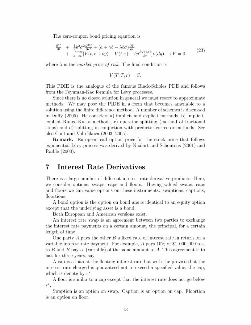
The zero-coupon bond pricing equation is

∂V

∂t+

1

2b2∂2V

∂r2+ (a− λb)∂V

∂r− rV = 0, (21)

where the function λ is often called the market price of risk. The finalcondition is

V (T, T, r) = Z.

This PDE may be solved approximately by standard numerical methods, see,for example, Wilmott, Howison and Dewynne (1995).

Remark. To price options on bonds with coupon, the reader is referredto Jamshidian (1989) and El Karoui and Rochet (1989).

6.3 Levy Bond Pricing for One-Factor SIRMs via CTMand Fourier Transform

We model the zero-coupon bond price with the following process (see Eberleinand Raible (1999), Raible (2000)):

P (t, T ) = P (0, T ) exp[

∫ T

0

r(s)ds]exp[

∫ t0σ(s, T )dL(s)]

Eexp[∫ t

0σ(s, T )dL(s)]

,

where r(t) has one of the representations in section 5.3.Eberlein and Raible (1999) derived the bond price process in the form

P (t, T ) = P (0, T ) exp[

∫ T

0

r(s)ds]exp[

∫ t0σ(s, T )dL(s)]

exp[∫ t

0θ(σ(s, T ))dL(s)]

,

where θ(u) := log(E[exp(uL(1))]) denotes the logarithm of the moment-generating function of the Levy process at time 1. For example, in the

11

classical Gaussian model we choose θ(u) = u2/2 and L(s) = W (s). We note,that we know the expressions for r(t) in the above formula for many SIRMs,see section 5.3.

Except when L(t) is a Poisson or a Brownian motion, our Levy marketmodel is an incomplete model. It means that there are many different equiv-alent martingales measures to choose. In general this leads to many differentpossible prices for European options or bond options, etc.

One of the way to price bond is to use for the P ∗ in (19) the Esschertransform equivalent martingale measure. Following Gerber and Shiu (1994),we can by using the so-called Esscher transform find in some cases at leastone equaivalent martingale measure P ∗. Let f(t, x) be the density of ourmodel’s (real world, i.e. under P ) distribution of L(t). For some real numberθ ∈ θ ∈ R|

∫ +∞−∞ exp(θy)f(t, y)dy < +∞ we can define a new density

f (θ)(t, x) =exp(θx)f(t, x)∫ +∞

−∞ exp(θy)f(t, y)dy.

In order to assume finiteness of the expectation in the denominator above inthe case of general Levy processes, we assume that∫

|x|>1exp[vx]ν(dx) <∞, for |v| < (1 + ε)M,

where ε > 0 and M is such that 0 ≤ σ(s, T ) ≤ M (a.s.) (see (8) and(9)) for 0 ≤ s ≤ T and ν(dx) is the Levy measure of L1. Typical choicesof this Levy process are the variance gamma, the normal inverse Gaussian,the generalized hyperbolic, the Meixner or CGMY processes (see Schoutens(2003)). Another way to price bond is to consider characteristic function(or Fourier transform), if it is known, of the risk-neutral log returns (seeCarr and Madan (1998)). We note, that if we know the explicit expressionfor r(t) (see section 5.3), then we can find the characteristic function of therisk-neutral bond price.

6.4 Levy Bond Pricing via PIDE

One more way to price bond is to consider the solution of a partial differen-tial integral equation with boundary condition, all in terms of the triplet ofLevy characteristics [γ, σ, νP

∗(dy)] of the Levy process under the risk-neutral

measure P ∗.Consider V (t, T, r)-bond price at time t, where interest rate r(t) follows

the following SDE (in general form)

dr(t) = a(r, t)dt+ b(r, t)dL(t), (22)

L(t) is a Levy process.For example, for GBM, a = µr and b = σr, for OU process, a = −µr and

b = σ, and so on (see section 3.1).

12

The zero-coupon bond pricing eqaution is

∂V∂t

+ 12b2σ2 ∂2V

∂r2+ (a+ γb− λbσ)∂V

∂r

+∫ +∞−∞ [V (t, r + by)− V (t, r)− by ∂V (t,r)

∂r]ν(dy)− rV = 0,

(23)

where λ is the market price of risk. The final condition is

V (T, T, r) = Z.

This PDIE is the analogue of the famous Black-Scholes PDE and followsfrom the Feynman-Kac formula for Levy processes.

Since there is no closed solution in general we must resort to approximatemethods. We may pose the PIDE in a form that becomes amenable to asolution using the finite difference method. A number of schemes is discussedin Duffy (2005). He considers a) implicit and explicit methods, b) implicit-explicit Runge-Kutta methods, c) operator splitting (method of fractionalsteps) and d) splitting in conjuction with predictor-corrector methods. Seealso Cont and Voltchkova (2003, 2005).

Remark. European call option price for the stock price that followsexponential Levy process was derived by Nualart and Schoutens (2001) andRaible (2000).

7 Interest Rate Derivatives

There is a large number of different interest rate derivative products. Here,we consider options, swaps, caps and floors. Having valued swaps, capsand floors we can value options on these instruments: swaptions, captions,floortions.

A bond option is the option on bond ans is identical to an equity optionexcept that the underlying asset is a bond.

Both European and American versions exist.An interest rate swap is an agreement between two parties to exchange

the interest rate payments on a certain amount, the principal, for a certainlength of time.

One party A pays the other B a fixed rate of interest rate in return for avariable interest rate payment. For example, A pays 10% of $1, 000, 000 p.a.to B and B pays r (variable) of the same amount to A. This agreement is tolast for three years, say.

A cap is a loan at the floating interest rate but with the proviso that theinterest rate charged is quaranteed not to exceed a specified value, the cap,which is denote by r∗.

A floor is similar to a cap except that the interest rate does not go belowr∗.

Swaption is an option on swap. Caption is an option on cap. Floortionis an option on floor.

13

8 Pricing of Gaussian and Levy Bond Op-

tions

8.1 Pricing of Gaussian Bond Options

Let interest rate r(t) follows the following SDE (in general form)

dr(t) = a(r, t)dt+ b(r, t)dW (t), (24)

where W (t) is a standard Wiener process.Consider the European call bond option, with exercise price K and expity

date T, on a zero-coupon bond with maturity date TB ≥ T.To find the value of the call option on bond (to buy a bond) we proceed

with the following steps:1. To find the value of the bond: VB(r, t;TB), that satisfies the following

PDE:

∂VB∂t

+1

2b2∂2VB∂r2

+ (a− λb)∂VB∂r− rVB = 0. (25)

with the final conditionVB(r, TB;TB) = Z.

2.Let CB(r, t) be the value of the call option on this bond. Since CB alsodepends on the random walk r(t), it must satisfy equation (1) too:

∂CB∂t

+1

2b2∂2CB∂r2

+ (a− λb)∂CB∂r− rCB = 0. (26)

with the final condition

CB(r, T ) = max(VB(r, T ;TB)−K, 0).

Remark. These PDEs can be solved numerically using standard meth-ods, see Wilmott, Howison and Dewynne (1995).

8.2 Pricing of Levy Bond Options


dr(t) = a(r, t)dt+ b(r, t)dL(t), (27)

where L(t) is a Levy process.Consider the European Call Bond Option, with exercise price K and

expity date T, on a zero-coupon bond with maturity date TB ≥ T.To find the value of the call option on bond (to buy a bond) we proceed

with the following steps:1. To find the value of the bond: VB(r, t;TB), that satisfies the following

PIDE:

14

∂VB

∂t+ 1

2b2σ2 ∂2VB

∂r2+ (a+ bγ − λbσ)∂VB

∂r

+∫ +∞−∞ [VB(t, r + by)− VB(t, r)− by ∂VB(t,r)

∂r]ν(dy)− rVB = 0.

(28)

with the final conditionVB(r, TB;TB) = Z.

2. Let CB(r, t) be the value of the call option on this bond. Since CBalso depends on the random walk r(t), it must satisfy equation (27) too:

∂CB

∂t+ 1

2b2σ2 ∂2CB

∂r2+ (a+ bγ − λbσ)∂CB

∂r

+∫ +∞−∞ [CB(t, r + by)− CB(t, r)− by ∂CB(t,r)

∂r]ν(dy)− rCB = 0.

(29)with the final condition

CB(r, T ) = max(VB(r, T ;TB)−K, 0). (30)

Remark. One of the approach to solve this PDIE could be numericalusing different finite difference methods, see Duffy (2005).

9 Pricing of Swaps, Caps and Floors

9.1 Pricing of Swaps, Caps and Floors for GaussianIRMs


dr(t) = a(r, t)dt+ b(r, t)dW (t), (31)

where W (t) is a standard Wiener process.Pricing of Swaps. We consider to value such swaps in general. Suppose

that A pays the interest on an amount Z to B at a fixed rate r∗ and B paysinterest to A at the floating rate r. These payments continue until time TS.Denote the value of this swap to A by ZVS(r, t). We note, that in a time-stepdt A receives (r − r∗)Zdt. If we think of this payment as being similar to acoupon payment on a simple bond then we find that:

∂VS∂t

+1

2b2∂2VS∂r2

+ (a− λb)∂VS∂r− rVS + (r − r∗) = 0. (32)

with the final conditionVS(r, TS) = 0.

We note, that r can be greater or less than r∗ and so VS(r, t) need not bepositive.

15

Pricing of Caps. The loan of Z is to be paid back at time TC . The valueof the capped loan, ZVC(r, t) satisfies the following PDE:

∂VC∂t

+1

2b2∂2VC∂r2

+ (a− λb)∂VC∂r− rVC + min(r, r∗) = 0. (33)

with the final conditionVC(r, TC) = 1.

Pricing of Floors. The value of the floored loan, ZVF (r, t), satisfies thefollowing PDE:

∂VF∂t

+1

2b2∂2VF∂r2

+ (a− λb)∂VF∂r− rVF + max(r, r∗) = 0. (34)

with the final conditionVF (r, TF ) = 1,

where TF is an expiry time for floor.Remark. These PDE can be solved numerically using standard methods,

see Wilmott, Howison and Dewynne (1995).

9.2 Pricing of Swaps, Caps and Floors for Levy IRMs

Consider V (r, t)-bond price at time t, where interest rate r(t) follows thefollowing SDE (in general form)

dr(t) = a(r, t)dt+ b(r, t)dL(t), (35)

L(t) is a Levy process.Pricing of Swaps. We consider to value such swaps in general. Suppose

that A pays the interest on an amount Z to B at a fixed rate r∗ and B paysinterest to A at the floating rate r. These payments continue until time TS.Denote the value of this swap to A by ZVS(r, t). We note, that in a time-stepdt A receives (r − r∗)Zdt. If we think of this payment as being similar to acoupon payment on a simple bond then we find that:

∂VS

∂t+ 1

2b2σ2 ∂2VS

∂r2+ (a+ bγ − λbσ)∂VS

∂r

+∫ +∞−∞ [VS(t, r + by)− VS(t, r)− by ∂VS(t,r)

∂r]ν(dy)

− rVS + (r − r∗) = 0.

(36)


We note, that r can be greater or less than r∗ and so VS(r, t) need not bepositive.

Pricing of Caps. The loan of Z is to be paid back at time TC . The valueof the capped loan, ZVC(r, t) satisfies the following PIDE:

∂VC

∂t+ 1

2b2σ2 ∂2VC

∂r2+ (a+ bγ − λbσ)∂VC

∂r

+∫ +∞−∞ [VC(t, r + by)− VC(t, r)− by ∂VC(t,r)

∂r]ν(dy)

− rVC + min(r, r∗) = 0.

(37)

16


Pricing of Floors. The value of the floored loan, ZVF (r, t), satisfies thefollowing PDE:

∂VF

∂t+ 1

2b2σ2 ∂2VF

∂r2+ (a+ bγ − λbσ)∂VF

∂r

+∫ +∞−∞ [VF (t, r + by)− VF (t, r)− by ∂VF (t,r)

∂r]ν(dy)

− rVF + max(r, r∗) = 0.

(38)

with the final conditionVF (r, TF ) = 1,

where TF is an expiry time for floor.Remark. One of the approach to solve thess PDIEs could be numerical

using different finite difference methods, see Duffy (2005).

10 Pricing of Swaptions, Captions and Floor-

tions

10.1 Pricing of Swaptions, Captions and Floortions forGaussian IRMs


dr(t) = a(r, t)dt+ b(r, t)dW (t), (39)

where W (t) is a standard Wiener process.Pricing of Swaptions. Consider European Swap Call Option, option

to buy this swap (a call swaption) for an amount K at time T < TS, whereTS is an expiry time for swap with value VS(r, t), t ≤ TS. Thus, this value VSsatisfies the following PDE (see (32)):

∂VS∂t

+1

2b2∂2VS∂r2

+ (a− λb)∂VS∂r− rVS + (r − r∗) = 0. (40)


Then the value CS(r, t) of this call swap option (call swaption) satisfiesthe following PDE:

∂CS∂t

+1

2b2∂2CS∂r2

+ (a− λb)∂CS∂r− rCS = 0. (41)


CS(r, T ) = max(VS(r, T )−K, 0). (42)

17

We solve for the value of the swap first and then use this value as the finaldata for the value of the swaption.

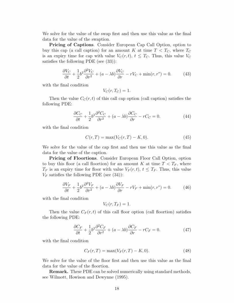
Pricing of Captions. Consider European Cap Call Option, option tobuy this cap (a call caption) for an amount K at time T < TC , where TCis an expiry time for cap with value VC(r, t), t ≤ TC . Thus, this value VCsatisfies the following PDE (see (33)):

∂VC∂t

+1

2b2∂2VC∂r2

+ (a− λb)∂VC∂r− rVC + min(r, r∗) = 0. (43)


Then the value CC(r, t) of this call cap option (call caption) satisfies thefollowing PDE:

∂CC∂t

+1

2b2∂2CC∂r2

+ (a− λb)∂CC∂r− rCC = 0. (44)


C(r, T ) = max(VC(r, T )−K, 0). (45)

We solve for the value of the cap first and then use this value as the finaldata for the value of the caption.

Pricing of Floortions. Consider European Floor Call Option, optionto buy this floor (a call floortion) for an amount K at time T < TF , whereTF is an expiry time for floor with value VF (r, t), t ≤ TF . Thus, this valueVF satisfies the following PDE (see (34)):

∂VF∂t

+1

2b2∂2VF∂r2

+ (a− λb)∂VF∂r− rVF + min(r, r∗) = 0. (46)

with the final conditionVC(r, TF ) = 1.

Then the value CF (r, t) of this call floor option (call floortion) satisfiesthe following PDE:

∂CF∂t

+1

2b2∂2CF∂r2

+ (a− λb)∂CF∂r− rCF = 0. (47)


CF (r, T ) = max(VF (r, T )−K, 0). (48)

We solve for the value of the floor first and then use this value as the finaldata for the value of the floortion.

Remark. These PDE can be solved numerically using standard methods,see Wilmott, Howison and Dewynne (1995).

18

10.2 Pricing of Swaptions, Captions and Floortions forLevy IRMs

Consider V (r, t)-bond price at time t, where interest rate r(t) follows thefollowing SDE (in general form)

dr(t) = a(r, t)dt+ b(r, t)dL(t), (50)

L(t) is a Levy process.Pricing of Swaptions. Consider European Swap Call Option, option

to buy this swap (a call swaption) for an amount K at time T < TS, whereTS is an expiry time for swap with value VS(r, t), t ≤ TS. Thus, this value VSsatisfies the following PIDE (see (36)):

∂VS

∂t+ 1

2b2σ2 ∂2VS

∂r2+ (a+ bγ − λbσ)∂VS

∂r

+∫ +∞−∞ [VS(t, r + by)− VS(t, r)− by ∂VS(t,r)

∂r]ν(dy)

− rVS + (r − r∗) = 0.

(51)


Then the value CS(r, t) of this call swap option (call swaption) satisfiesthe following PIDE:

∂CS

∂t+ 1

2b2σ2 ∂2CS

∂r2+ (a+ bγ − λbσ)∂CS

∂r

+∫ +∞−∞ [CS(t, r + by)− CS(t, r)− by ∂CS(t,r)

∂r]ν(dy)− rCS = 0.

(52)


CS(r, T ) = max(VS(r, T )−K, 0). (53)

We solve for the value of the swap first and then use this value as the finaldata for the value of the swaption.

Pricing of Captions. Consider European Cap Call Option, option tobuy this cap (a call caption) for an amount K at time T < TC , where TCis an expiry time for cap with value VC(r, t), t ≤ TC . Thus, this value VCsatisfies the following PIDE (see (37)):

∂VC

∂t+ 1

2b2σ2 ∂2VC

∂r2+ (a+ bγ − λbσ)∂VC

∂r

+∫ +∞−∞ [VC(t, r + by)− VC(t, r)− by ∂VC(t,r)

∂r]ν(dy)

− rVC + min(r, r∗) = 0.

(54)


Then the value CC(r, t) of this call cap option (call caption) satisfies thefollowing PDE:

∂CC

∂t+ 1

2b2σ2 ∂2CC

∂r2+ (a+ bγ − λbσ)∂CC

∂r

+∫ +∞−∞ [CC(t, r + by)− CC(t, r)− by ∂CC(t,r)

∂r]ν(dy)− rCC = 0.

(55)

19


C(r, T ) = max(VC(r, T )−K, 0). (56)

We solve for the value of the cap first and then use this value as the finaldata for the value of the caption.

Pricing of Floortions. Consider European Floor Call Option, optionto buy this floor (a call floortion) for an amount K at time T < TF , whereTF is an expiry time for floor with value VF (r, t), t ≤ TF . Thus, this valueVF satisfies the following PIDE (see (38)):

∂VF

∂t+ 1

2b2σ2 ∂2VF

∂r2+ (a+ bγ − λbσ)∂VF

∂r

+∫ +∞−∞ [VF (t, r + by)− VF (t, r)− by ∂VF (t,r)

∂r]ν(dy)

− rVF + min(r, r∗) = 0.

(57)

with the final conditionVC(r, TF ) = 1.

Then the value CF (r, t) of this call floor option (call floortion) satisfiesthe following PIDE:

∂CF

∂t+ 1

2b2σ2 ∂2CF

∂r2+ (a+ γ − λbσ)∂CF

∂r

+∫ +∞−∞ [CF (t, r + y)− CF (t, r)− y ∂CF (t,r)

∂r]ν(dy)− rCF = 0.

(58)


CF (r, T ) = max(VF (r, T )−K, 0). (59)

We solve for the value of the floor first and then use this value as the finaldata for the value of the floortion.

Remark. One of the approach to solve these PDIEs could be numericalusing different finite difference methods, see Duffy (2005).

11 Conclusion

We discussed how to calculate the price of zero-coupon bonds for many Gaus-sian and Levy one-factor and multi-factor models of r(t) using change of timemethod. These models include, in particular, Ornshtein-Uhlenbeck (1930),Vasicek (1977), Cox-Ingersoll-Ross (1985), continuous-time GARCH, Ho-Lee(1986), Hull-White (1990) and Heath-Jarrrow-Morton (1992) models andtheir various combinations. We also derive PDIE for the values of swaps,caps, floors and options on them, swaptions, captions and floortions, re-spectively. We apply the change of time method to price the interest ratederivatives for the interest rates r(t) described by various stochastic differ-ential equations driven by α-stable Levy processes. We could also apply thesame techniques, i.e., change of time and PIDE, to price many interest ratederivatives for multi-factor Gaussian and Levy interest rate models. But thisdiscussion is outside the scope of this paper and will be considered in thefuture research paper, as well as the numerical solutions of PIDEs presentedin the paper.

20

Acknowledgement.

This research is supported by NSERC. I would like to thank the organizersof the 2008 Stochastic Modelling Symposium for their invitation to presentthe paper. All the remaining errors are mine.

12 Appendix A: One-Factor and Multi-Factor

Gaussian Interest Rate Models

12.1 One-Factor Gaussian SIRMs

1. The Geometric Brownian Motion Model (Rendleman andBartter (1980)). dr(t) = µr(t)dt+ σr(t)dW (t).

2. The Ornstein-Uhlenbeck (1930) Model. dr(t) = −µr(t)dt +σdW (t),

3. The Vasicek (1977) Model. dr(t) = µ(b− r(t))dt+ σdW (t).4. The Continuous-Time GARCH Model. dr(t) = µ(b− r(t))dt+

σr(t)dW (t).5. The Cox-Ingersoll-Ross (1985) Model. dr(t) = k(θ−r(t))dt+

γ√rdW (t).6. The Ho and Lee (1986) Model. dr(t) = θ(t)dt+ σdW (t).7. The Hull and White (1990) Model. dr(t) = (a(t)−b(t)r(t))dt+

σ(t)dW (t)8. The Heath, Jarrow and Morton (1987) Model. Define the

forward interest rate f(t, s), for t ≤ s, characterized by the following equalityP (t, u) = exp[−

∫ utf(t, s)ds] for any maturity u. f(t, s) represents the instan-

teneous interest rate at time s as ‘anticipated‘ by the market at time t. Itis natural to set f(t, t) = r(t). The process f(t, u)0≤t≤u satisfies an equation

f(t, u) = f(0, u) +∫ t

0a(v, u)dv +

∫ t0b(f(v, u))dW (v), where the processes a

and b are continuous. We note, that the lasr SDE may be written in thefollowing form: df(t, u) = b(f(t, u))(

∫ utb(f(t, s)))ds+ b(f(t, u))dW (t), where

W (t) = W (t)−∫ t

0q(s)ds and q(t) =

∫ utb(f(t, s))ds− a(t,u)

b(f(t,u)).

12.2 Multi-Factor Gaussian SIRMs

Multi-factor models driven by Brownian motions can be obtained using var-ious combinations of above-mentioned processes. We give one example oftwo-factor continuous-time GARCH SIRM:

dr(t) = µ(b(t)− r(t))dt+ σr(t)dW 1(t)db(t) = ξb(t)dt+ ηb(t)dW 2(t),

where W 1,W 2 may be correlated, µ, ξ ∈ R, σ, η > 0.

21

13 Appendix B: Solutions to the One-Factor

and Multi-Factor Gaussian Interest Rate

Models

13.1 Solution of One-Factor Gaussian SIRMs UsingCTM

We use change of time method (see Ikeda and Watanabe (1981)) to getthe solutions to the following below equations (see Swishchuk (2007)). W (t)below is an standard Brownian motion, and W is a (Tt)t∈R+-adapted standard

Brownian motion on (Ω,F , (Ft)t∈R+ , P ).1. Geometric Brownian Motion. dr(t) = µr(t)dt + σr(t)dW (t).

Solution r(t) = eµt[r(0) + W (Tt)], where Tt = σ2∫ t

0[r(0) + W (Ts)]

2ds.2. Ornstein-Uhlenbeck Process. dr(t) = −µr(t)dt + σdW (t), So-

lution r(t) = e−µt[r(0) +W (Tt)], where Tt = σ2∫ t

0(eµs[r(0) +W (Ts)])

2ds.3. Vasicek Process. dr(t) = µ(b − r(t))dt + σdW (t), solution r(t) =

e−µt[r(0)− b+ W (Tt)], where Tt = σ2∫ t

0(eµs[r(0)− b+ W (Ts)] + b)2ds.

4. Continuous-Time GARCH Process. dr(t) = µ(b − r(t))dt +σr(t)dW (t). Solution r(t) = e−µt(r(0)−b+W (Tt))+b, where Tt = σ2

∫ t0[r(0)−

b+ W (Ts) + eµsb)2ds.5. Cox-Ingersoll-Ross Process. dr2(t) = k(θ−r2(t))dt+γr(t)dW (t),

solution r2(t) = e−kt[r20 − θ2 + W (Tt)] + θ2, where Tt = γ−2

∫ t0[ekTs(r2

0 − θ2 +

W (s)) + θ2e2kTs ]−1ds.6. Ho and Lee Process. dr(t) = θ(t)dt + σdW (t). Solution r(t) =

r(0) + W (σ2t) +∫ t

0θ(s)ds.

7. Hull and White. dr(t) = (a(t)− b(t)r(t))dt+ σ(t)dW (t). Solution

r(t) = exp[−∫ t

0b(s)ds][r(0)− a(s)

b(s)+ W (Tt)], where Tt =

∫ t0σ2(s)[r(0)− a(s)

b(s)+

W (Ts) + exp[∫ s

0b(u)du]a(s)

b(s)]ds.

8. Heath, Jarrow and Morton. f(t, u) = f(0, u) +∫ t

0a(v, u)dv +∫ t

0b(f(v, u))dW (v). Solution f(t, u) = f(0, u) + W (Tt) +

∫ t0a(v, u)dv, where

Tt =∫ t

0bα(f(0, u) + W (Ts) +

∫ s0a(v, u)dv)ds.

13.2 Solution of Multi-Factor Gaussian SIRMs UsingCTM

Solution of multi-factor models driven by Brownian motions can be obtainedusing various combinations of solutions of the above-mentioned processes, seesubsection 5.1, and CTM. We give one example of two-factor Continuous-Time GARCH model driven by Brownian motions:

dr(t) = µ(b(t)− r(t))dt+ σr(t)dW 1(t)db(t) = ξb(t)dt+ ηb(t)dW 2(t),

22

where W 1,W 2 may be correlated, µ, ξ ∈ R, σ, η > 0.Solution, using CTM for the first and the second equations, subsection

13.1: r(t) = e−µt[r(0)− eξt(b(0) + W 2(T 2t )) + W 1(T 1

t )] + eξt[b(0) + W 2(T 2t )],

where T i are defined in 4. (i = 1) and 1. (i = 2), respectevely, subsection13.1. Here, W 1(t) and W 2(t) are independent.

References

D. Applebaum. Levy Processes and Stochastic Calculus, Cambridge Uni-versity Press, 2003.

N. Bingham and R. Kiesel. Risk-Neutral Valuations, Pricing and Hedgingof Financial Derivatives, Springer Finance, London, 1998.

T. Bjork, Y. Kabanov, and W. Rungaldier. Bond market structure in thepresence of marked point process, Math. Finance, 1997, 7, 211-239.

T. Bjork. Arbitrage Theory in Continuous Time, Oxford UniversityPress, 1998.

F. Black, E. Derman and W. Toy. A one-factor model of interest ratesand its applications to treasury bond options, Fin. Anal. J., 1990, 46(1),33-39.

F. Black and P. Karasinski. Bond and option pricing when short ratesare lognormal, Fin Anal. J., 1991, 47(4), 52-59.

A. Brace, D. Gatarek and M. Musiela. The market model of interest ratedynamics, Math. Finance, 1997, 4, 127-155.

D. Brigo and F. Mercurio. Interest Rate Models: Theory and Practice,Springer, 2001.

M. Brennan and E. Schwartz. A continuous time approximation to thepricing of bonds. Journal of of Banking and Finance, 1979, pp. 133-155.

P. Carr and D. Madan. Option valuation using the fast Fourier trans-form, Journal of Computational Finance, 2, 61-73, 1998.

K. Chan, A. Karoly, F. Longstaff and A. Sanders. An empirical compar-ison of alternative models of the short-term interest rate, J. Fin., 1992, 47,1209-1227.

R. Cont and E. Voltchkova. Integor-differential equations for option pric-ing in exponential Levy models, Finance and Stochastics, 9, 299-325, 2005.

R. Cont and E. Voltchkova. A finite difference scheme for option pricingin jump diffusion and exponential Levy models, Internal Report CMAP, No.513, September 2003.

G. Courtadon. The pricing of options on default-free bonds. J. of Finan-cial and Quant. Analysis, 17 (1982), pp. 301-329.

J. Cox,J.Ingersoll and S.Ross. A theory of the term structure of interestrate. Econometrics, 53 (1985), pp. 385-407.

Q. Dai, K. Singleton. Specification analysis of affine term structure mod-els, J. Fin., 2000, 55, 1943-1978.

23

S. Das. A discrete-time approach to Poisson-Gaussian bond option pric-ing in the Heath-Jarrow-Morton model, J. Econ. Dynam. Control, 1999, 23,333-369.

S. Das and S. Foresi. Exact solutions for bond and option prices withsystematic jump risk, Rev. Derivatives Res., 1996, 1, 7-24.

D. Duffie. Dynamic Asset Pricing Theory, Princeton University Press,Princeton, NJ, 1992.

D. Duffie and R. Kan. A yield-factor model of interest rate, Math. Fin.,1994, 4, 379-406.

D. Duffie and R. Kan. Multi-factor term structure models, Philos. Trans.R. Soc. London, Ser. A, 1994, 347, 577-586.

D. Duffie, J. Pan and K. Singleton. Transform analysis and option pric-ing for affine jump-diffusions, Econometrica, 2000, 68, 1343-1376.

D. Duffy. Numerical analysis of jump diffusion models: a partial differ-ential equation approach, Datasim, 2005.

D. Duffy. Finite Difference Methods in Financial Engineering: A PartialDifferential Approach. Wiley and Sons, Chichester, 2005.

E. Eberlein and S. Raible. Term structure models driven by general Levyprocesses. Mathematical Finance 9, 31-53, 1999.

D. Filipovic. Consistency Problems for Heath-Jarrow-Morton InterestRate Models. Lecture Notes in Mathematics, vol. 1760. Springer, 2001.

H. U. Gerber and E. S. W. Shiu. Option pricing by Esscher-transforms.Transactions of the Society of Actuaries, 46, 99-191, 1994.

P. Glasserman and S. Kou. The term structure of simple forward rateswith jump risk, Math. Fin., 2003, 13, 383-410.

P. Glasserman and N. Merener. Numerical solution of jump diffusionLIBOR market models, Fin. Stochastics, 2003, 7, 1-27.

D. Hearth,R.Jarrow and A.Morton. Bond pricing and the term structureof the interest rates: A new mathodology. Econometrica, 60, 1 (1992), pp.77-105.

J. Hull and A.White. Pricing interest rate derivative securities. Reviewof Fin. Studies, 3,4 (1990), pp. 573-592.

T.S.Y. Ho and S.-B. Lee. Term structure movements and pricing interestrate contigent claim. J. of Finance, 41 (December 1986), pp. 1011-1029.

N. Ikeda and S.Watanabe. Stochastic Differential Equations and DiffusionProcesses. North-Holland/Kodansha Ltd., Tokyo, 1981.

J. Jacod and A. Shiryaev. Limit Theorems for Stochastic Processes,Springer-Verlag, 1987; second edition (2003).

J. James and N. Webber. Interest Rate Modelling. John Wiley & Sons,Ltd., 2002.

F. Jamshidian. An exact bond option pricing formula. J. of Finance, 44(March 1989), pp. 205-209.

F. Jamshidian. LIBOR and swap market models and measures, Fin.Stochastics, 1, 293-330.

24

D. Jara. An extension of Levy theorem and application to financial mod-els based on futures prices, PhD dissertation, Dept. of Math. Sciences,Carnegie Mellon University, 2000.

D. Lamperton and B.Lapeyre. Introduction to Stochastic Calculus Ap-plied to Finance, Chapman&Hall, 1996.

F. Longstaff and E. Schwartz. Interest rate volatility and the term struc-ture: A two-factor general equilibrium model, J. Finance, 47(4): 1259-82.

Y. Maghsoodi. Solution of the extended CIR term structure and bondoption valuation, Math. Fin., 1996, 6, 89-109.

K. Miltersen, S. Sandmann and D. Sondermann. Closed form solutionsfor term structure derivatives with log-normal interest rates, J. Finance, 52,409-430.

D. Nualart and W. Schoutens. Backwards SDE and Feynman-Kac for-mula for Levy processes, with application in finance, Bernoulli, 7, 761-776.

L. Ornstein and G.Uhlenbeck. On the theory of Brownian motion. Phys-ical Review, 36 (1930), 823-841.

A. Pelsser. Efficient Methods for Valuing Interest Rate Derivatives, Springer,Berlin, 2000.

S. Raible. Levy processes in finance: theory, numerics, and empiricalfacts. PhD thesis, Freiburg, 2000.

R. Rebonato. Modern Pricing of Interest-Rate Derivatives: The LIBORMarket Model and Beyond, Princeton University Press, Princeton, NJ, 2000.

R. Rebonato. Interest-Rate Option Models. John Wiley & Sons, Ltd.,1996.

R. Rendleman and B. Barttler. The pricing of options on debt securities,Journal of Financial and Quantitative Analysis, 15 (March 1980), 11-24.

J. Rosinski and W. Woyczynski. On Ito stochastic integration with re-spect to p-stable motion: inner clock, integrability of sample paths, doubleand multiple integrals, Ann. Probab. 14, 271-286, 1986.

K. Sato. Levy Processes and Infinitely Divisible Distributions. Cam-bridge Studies in Advanced Mathematics, vol. 68. Cambridge UniversityPress, 1999.

S. Schaefer and E.Schwartz. Time-dependent and the pricing of options.J. of Finance,, 42 (December 1987), pp. 1113-1128.

H. Shirakawa. Interest rate option pricing with Poisson-Gaussian forwardrate curve processes, Math. Fin., 1991, 1, 77-94.

O. Vasicek. An equilibrium characterization of the term structure. J. ofFinan. Economics, 5 (1977), pp. 177-188.

W. Schoutens. Levy Processes in Finance. Pricing Financial Derivatives.Wiley & Sons, 2003.

A. Swishchuk. Modeling of Variance and Volatility Swaps for FiancialMarkets with Stochastic Volatility, WILMOTT Magazine, 2004, SeptemberIssue, Technical Article No 2, pp. 64-72.

A. Swishchuk. Change of time method in mathematical finance, Canad.Appl. Math. Quart., vol. 15, No. 3, 2007, 32p.

25

P. Wilmott, J. Dewynne and S. Howison. The Mathematics of FinancialDerivatives. A Student Introduction, Cambridge University Press, 1995.

26

Documents

L evy-Based Interest Rate Derivatives: Change of …people.ucalgary.ca/~aswish/SwishSMS08MontPaper.pdf · L evy-Based Interest Rate Derivatives: Change of Time Method and PIDEs