KPZ limit for interacting particle systems

—Introduction—

Tadahisa Funaki (舟木 直久)

Waseda University (早稲田大学)

November 17th+19th, 2020

Yau Mathematical Sciences Center, Mini-Course, Nov 17-Dec 17, 2020Lecture No 1

1 / 40

Plan of the course (10 lectures)

1 Introduction

2 Supplementary materialsBrownian motion, Space-time Gaussian white noise,(Additive) linear SPDEs, (Finite-dimensional) SDEs,Martingale problem, Invariant/reversible measures forSDEs, Martingales

3 Invariant measures of KPZ equation (F-Quastel, 2015)

4 Coupled KPZ equation by paracontrolled calculus(F-Hoshino, 2017)

5 Coupled KPZ equation from interacting particle systems(Bernardin-F-Sethuraman, 2020+)

5.1 Independent particle systems5.2 Single species zero-range process5.3 n-species zero-range process5.4 Hydrodynamic limit, Linear fluctuation5.5 KPZ limit=Nonlinear fluctuation

2 / 40

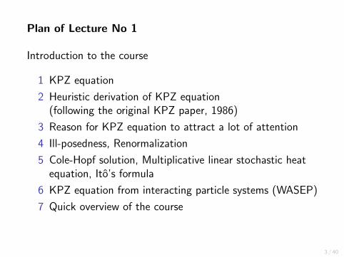
Plan of Lecture No 1

Introduction to the course

1 KPZ equation

2 Heuristic derivation of KPZ equation(following the original KPZ paper, 1986)

3 Reason for KPZ equation to attract a lot of attention

4 Ill-posedness, Renormalization

5 Cole-Hopf solution, Multiplicative linear stochastic heatequation, Ito’s formula

6 KPZ equation from interacting particle systems (WASEP)

7 Quick overview of the course

3 / 40

1. KPZ equation

The KPZ (Kardar-Parisi-Zhang, 1986) equation describesthe motion of growing interface with random fluctuation.

(Takeuchi-Sano-Sasamoto-Spohn)

(Right Fig) h = h(t, x) ∈ R denotes height of interfacemeasured from the x-axis at time t and position x .

Video of combustion experiment by Laser shot:srep00034-s2.mov, srep00034-s3.mov (Takeuchi-Sano)

4 / 40

KPZ is an equation for height function h(t, x):

∂th = 12∂2xh +

12(∂xh)

2 + W (t, x), x ∈ T (or R). (1)

where T ≡ R/Z = [0, 1). We consider in 1D on a whole line R or on a finite

interval T under periodic boundary condition. The coefficients 1

2are not important, since we can change

them under some scaling. W (t, x) is a space-time Gaussian white noise with mean 0

and covariance structure:

E [W (t, x)W (s, y)] = δ(t − s)δ(x − y). (2)

This means that the noise is independent if (t, x) isdifferent, since “Gaussian property+0-correlation” meansindependence.

However, W (t, x) is realized only as a generalizedfunction (distribution).

5 / 40

2. Heuristic derivation of KPZ equation We give a derivation of KPZ equation following the

original KPZ paper 1986. Consider a motion of interface (curve) growing upward

with normal velocity:

V = κ+ A,

where κ is the (signed) curvature and A > 0 is a constant.

6 / 40

The interface dynamics can be described by an equationfor its height function h(t, x) assuming that the interfacein R2 is represented as a graph:

γt = (x , y); y = h(t, x), x ∈ R ⊂ R2.

The dynamics “V = κ+ A” can be rewritten into thefollowing nonlinear PDE for h(t, x)

∂th =∂2xh

1 + (∂xh)2+ A(1 + (∂xh)

2)1/2 (3)

7 / 40

Indeed, (3) can be derived as follows.

First, note that the normal vectorn to the curve

γh = (x , y); y = h(x), x ∈ R ⊂ R2

at the point (x , y) is given by

n=

1(1 + (∂xh(x))2

)1/2 (−∂xh(x)1

)

pf)n⊥

(1

∂xh(x)

)(= tangent vector to γh) and |

n | = 1.

The interface growth to the directionn is equivalent to

the growth of the height function h to the vertical

directionm, where

m=

(0(

1 + (∂xh(x))2)1/2)

pf) We can check (m −

n) ⊥n

8 / 40

The curvature of the curve γh = y = h(x) at (x , y) isgiven by

κ =∂2xh(x)(

1 + (∂xh(x))2)3/2 .

Summarizing these observations, the interface growingequation V = κ+ A can be written as

∂th =

∂2xh

(1 + (∂xh)2)3/2+ A

(1 + (∂xh)

2)1/2,

i.e. we obtain (3):

∂th =∂2xh

1 + (∂xh)2+ A(1 + (∂xh)

2)1/2,

for the height function h = h(t, x).

9 / 40

If we consider h := h− At instead of h by subtracting theconstant growth factor At and write h for h again, weobtain that

∂th =∂2xh

1 + (∂xh)2+ A

(1 + (∂xh)

2)1/2 − 1

≃ ∂2xh +

A2(∂xh)

2,

i.e.

∂th= ∂2xh +

A2(∂xh)

2,

at least if |∂xh| is small, i.e., if we take the leading effectof this equation.

Note that u := ∂xh is a solution of (viscous) Burgersequation:

∂tu = ∂2xu + A

2∂xu

2.

10 / 40

Kardar-Parisi-Zhang equation (KPZ, 1986) is obtained bytaking the fluctuation effect due to space-timeindependent noise W (t, x) into account:

∂th = 12∂2xh +

12(∂xh)

2 + W (t, x).

Here h = h(t, x , ω) and W (t, x) = W (t, x , ω) is thespace-time Gaussian white noise defined on a certainprobability space (Ω,F ,P) with mean 0 and covariancestructure

E [W (t, x)W (s, y)] = δ(x − y)δ(t − s).

We took A = 1 and put 12in front of ∂2

xh. Only leading terms are taken in the equation. This simplification is essential in view of the scaling

property or universality related to the KPZ equation.

Mathematically, everything is built on a probability space (Ω,F ,P), i.e.Ω is a set, F is a σ-field of Ω, P is a measure on (Ω,F) s.t. P(Ω) = 1.

11 / 40

3. Reason for KPZ equation to attract a lot of attention

13-power law (instead of 1

2-law in usual CLT): Fluctuation

of height function at a single point x = 0:

h(t, 0) ≍ c1t + c2t13 ζTW ,

in particular, Var(h(t, 0)) = O(t23 ), as t → ∞, i. e. the

fluctuations of h(t, 0) are of order t13 . Subdiffusive

behavior different from CLT (=diffusive behavior).

The limit distribution of h(t, 0) under scaling is given bythe so-called Tracy-Widom distribution ζTW (differentdepending on initial distributions). (instead of Gaussiandistribution in CLT)

KPZ universality class, 1:2:3 scaling, KPZ fixed point

Integrable Probability

12 / 40

Singular ill-posed SPDEs:

- Hairer: Regularity structures, KPZ equation, dynamicP(ϕ)d -model, Parabolic Anderson model

- Gubinelli-Imkeller-Perkowski: Paracontrolled calculus(harmonic analytic method)

- The solution map is continuous in “W ε and their(finitely many) polynomials”.

- Renormalization is required (called subcritical case).

Microscopic interacting particle systems

- Bertini-Giacomin (1997) was the first to this direction.- This is one of main purposes of this course.

13 / 40

4. Ill-posedness, Renormalization

Nonlinearity and roughness ofnoise conflictwith eachother. W (t, x) ∈ C− d+1

2− := ∩

δ>0C− d+1

2−δ a.s. if x ∈ Td or Rd .

(Construction will be discussed later → Lecture No 2). Cα: (Holder-)Besov space with exponent α ∈ R. The linear SPDE (d = 1): (Schauder effect)

∂th = 12∂2xh + W (t, x), x ∈ T

obtained by dropping the nonlinear term has a solutionh ∈ C

14−, 1

2−([0,∞)× T) := ∩

δ>0C

14−δ, 1

2−δ([0,∞)× T) a.s.

(This will be discussed later → Lecture No 2). Therefore, no way to define the nonlinear term (∂xh)

2 in(1) in a usual sense.

Actually, it requires a renormalization. The followingRenormalized KPZ equation with compensatorδx(x) (= +∞) would have a meaning (cf. Cole-Hopfsolution):

∂th = 12∂

2xh + 1

2(∂xh)2 − δx(x)+ W (t, x).

14 / 40

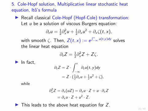
5. Cole-Hopf solution, Multiplicative linear stochastic heatequation, Ito’s formula

Recall classical Cole-Hopf (Hopf-Cole) transformation:Let u be a solution of viscous Burgers equation:

∂tu = 12∂2xu + 1

2∂xu

2 + ∂xζ(t, x),

with smooth ζ. Then, Z (t, x) := e∫ x−∞ u(t,y)dy solves

the linear heat equation

∂tZ = 12∂2xZ + Zζ.

In fact,∂tZ = Z ·

∫ x

−∞∂tu(t, y)dy

= Z · ( 12∂xu + 12u

2 + ζ),

while

∂2xZ = ∂x(uZ ) = ∂xu · Z + u · ∂xZ

= ∂xu · Z + u2 · Z .

This leads to the above heat equation for Z .15 / 40

Motivated by this and regarding u = ∂xh, consider the(multiplicative) linear stochastic heat equation (SHE) forZ = Z (t, x , ω):

∂tZ = 12∂

2xZ + ZW (t, x), x ∈ R, (4)

with a multiplicative noise (defined in Ito’s sense). The solution Z (t) of (4) can be defined in a generalized

functions’ sense or in a mild form (Duhamel’s formula):

Z (t, x) =

∫Rp(t, x , y)Z (0, y)dy+

∫ t

0

∫Rp(t−s, x , y)Z (s, y)dW (s, y),

where p(t, x , y) = 1√2πt

e−(y−x)2/(2t) is the heat kernel.

(4) in Ito’s sense is well-posed (→ see next page)

SHE (4) defined in Stratonovich sense:

∂tZ = 12∂

2xZ + Z W (t, x)

is ill-posed. (→ see below)

16 / 40

These two notions of solutions (in generalized functionsor mild) are equivalent, and ∃unique solution s.t.Z (t) ∈ C ([0,∞), Ctem) a.s., where

Ctem = Z ∈ C (R,R); ∥Z∥r < ∞,∀ r > 0,∥Z∥r = sup

x∈Re−r |x ||Z (x)|.

(Strong comparison) If Z (0, x) ≥ 0 for ∀x ∈ R andZ (0, x) > 0 for ∃x ∈ R, then Z (t) ∈ C ((0,∞), C+) a.s.,where C+ = C

(R, (0,∞)

).

Therefore, we can define the Cole-Hopf transformation:

h(t, x) := log Z (t, x). (5)

17 / 40

Heuristic derivation of the KPZ eq (with renormalization factorδx(x)) from SHE (4) under the Cole-Hopf transformation (5): (Finite-dimensional) Ito’s formula:

df (Xt) = f ′(Xt)dXt +12f ′′(Xt)(dXt)

2

for example, for Xt = Bt , (dBt)2 = dt.

In infinite-dimensional setting,

dW (t, x)dW (t, y) = δ(x − y)dt (= δx(y)dt)

By Ito’s formula, taking f (z) = log z under the C-Htransformation (5), we have

dh(t, x) = f ′(Z (t, x))dZ (t, x) + 12f ′′(Z (t, x))(dZ (t, x))2.

Note f ′(z) = (log z)′ = z−1, f ′′(z) = (log z)′′ = −z−2. Note also from SHE (4),

(dZ (t, x))2 = (Z (t, x)dW (t, x))2 = Z 2(t, x)δx(x)dt.

18 / 40

Therefore, writing ∂th for dh(t,x)dt

, we obtain

∂th = Z−1∂tZ − 12Z−2Z 2δx(x)

= Z−1(

12∂2xZ + ZW

)− 1

2δx(x) (by SHE (4))

= 12Z−1∂2

xZ + W − 12δx(x).

However, since h = log Z , a simple computation (as wealready saw for u = ∂xh) shows

Z−1∂2xZ = ∂2

xh + (∂xh)2 (= ∂xu + u2).

This leads to the KPZ eq with renormalization factor:

∂th = 12∂2xh +

12(∂xh)2 − δx(x)+ W (t, x). (6)

19 / 40

The function h(t, x) defined by (5) is meaningful andcalled the Cole-Hopf solution of the KPZ equation,although the equation (1) does not make sense.

Problem: To introduce approximations for (6), inparticular, well adapted to finding invariant measures.(→ F-Quastel, Lecture No 3)

Hairer gave a meaning to (6) without bypassing SHE.

Ito’s formula for Stratonovich integral has no Itocorrection term (i.e. the term with 1

2). If SHE defined in

Stratonovich sense were well-posed, we would obtainwell-posed KPZ equation. But, this is not true.

20 / 40

6. KPZ equation from interacting particle systems

One of our interests is to derive KPZ(-Burgers) equationfrom microscopic particle systems.

Bertini-Giacomin (1997): Derivation of Cole-Hopfsolution of KPZ equation from WASEP (weaklyasymmetric simple exclusion process)

For WASEP, Cole-Hopf transformation works even atmicroscopic level (Gartner).

21 / 40

6.1 WASEP (weakly asymmetric simple exclusion process)

WASEP (on Z) is a collection of infinite particles on Z. Each particle performs simple random walk with jump

rates 12to the right and 1

2+ δ to the left, under the

exclusion rule that at most one particle can occupy eachsite, where δ > 0 is a small parameter (weak asymmetry).

Configuration space: X = +1,−1Z σ = σ(x)x∈Z ∈ X and

σ(x) =+1

−1

⇐⇒

∃ particle at x

no particle at x

22 / 40

σx ,y ∈ X denotes a new configuration after exchangingvariables at x and y (i.e., if there is a particle at x and noparticle at y , σx ,y is the configuration after the particle atx jumps to y . Or a particle at y jumps to x if x isvacant.)

σx ,y (z) =

σ(y), if z = x ,

σ(x), if z = y ,

σ(z), otherwise.

(Infinitesimal) rate of transition σ 7→ σz,z+1, when thewhole configuration is σ, is given by

cz,z+1(σ) =121σ(z)=1,σ(z+1)=−1+(1

2+δ)1σ(z)=−1,σ(z+1)=1.

23 / 40

Generator: For a function f on X ,

Lf (σ) =∑z∈Z

cz,z+1(σ)f (σz,z+1)− f (σ).

The rate cz,z+1 can be decomposed as follows.

The rate that a particle makes a jump:λ = 1 + δ

(= 1

2+ (1

2+ δ)

) When a jump occurs,

p+ =12

1+δ: probability of jump to the right

p− =12+δ

1+δ: probability of jump to the left

Note that p+ + p− = 1 (i.e., p± is a probability), bynormalizing cz,z+1 by λ.

24 / 40

6.2 Construction of interacting particle systems (in general)

Particle system is a continuous-time (jump) Markovprocess σt ≡ σt(ω) on a configuration space X ofparticles.

Once infinitesimal rate c(σ) governing the random motionof particles is given, one can construct σt as follows.

[Distributional construction] c(σ) determines the generator of Markov process L We can construct corresponding semigroup etL on C (X ). By Markov property, etL determines finite-dimensional

distributions (joint distributions of Markov process atfinitely many times).

By Kolmogorov’s extension theorem+regularization ofpaths, this determines the distribution of the Markovprocess on the path space D([0,∞),X ), which denotesthe Skorohod space allowing jumps of functions.

Liggett, Interacting Particle Systems, Springer, 1985.25 / 40

[Pathwise construction] Each particle has its own “bell”. Bells are independent

and ring according to the exponential holding time:

P(T > t) = e−λt , t ≥ 0, λ > 0.

Since E [T ] = 1λ , “large λ” means that the bell rings

quickly. We write Td= exp(λ).

λ for each particle is determined from infinitesimal ratec(σ). (For WASEP, λ = 1 + δ)

When first bell rings, the corresponding particle makes ajump to a place chosen by certain probability p.(For WASEP, p±)

After this jump, whole system refreshes with all bells,and repeats the procedure.

We usually consider infinite particle system, and thisrequires careful construction of the system.

26 / 40

6.3 Hydrodynamic limit (LLN)

WASEP σt = (σt(x))x∈Z is constructed by the aboverecipe from cz,z+1(σ) with weak asymmetry δ.

We first study the hydrodynamic limit (HDL) for theWASEP σt taking δ = ε, where ε is the ratio ofmicroscopic/macroscopic spatial sizes.

As we will see, scalings in δ are different for HDL/KPZ.

Consider the macroscopic empirical measure of σt definedby small-mass and space-time-diffusive scaling:

Xt(du) = ε∑x∈Z

σε−2t(x)δεx(du), u ∈ R,

or equivalently, for a test function φ ∈ C∞0 (R),

⟨Xt , φ⟩ = ε∑x∈Z

σε−2t(x)φ(εx).

27 / 40

Theorem 1

Xt(du) −→ε↓0

α(t, u)du (in prob),

where α(t, u) is a solution of viscous Burgers equation:

∂tα = 12∂2uα + 1

2∂u(1− α2).

If α = ∂um, the equation for m is

∂tm = 12∂2um + 1

2(1− (∂um)2).

(KPZ type but without noise)

F-Sasada, CMP 299, 2010F, Lectures on Random Interfaces, SpringerBriefs, 2016, Theorem 2.7for relation to Vershik curve (introducing boundary).

28 / 40

Heuristic derivation of the limit equation

To show this theorem, we use Dynkin’s formula(→ Lecture No 2):

⟨Xt , φ⟩ = ⟨X0, φ⟩+∫ t

0

ε−2·ε∑x

(Lσ)ε−2s(x)φ(εx)ds+Mεt (φ).

ε−2 comes from the time change.

The contribution of the martingale term Mεt (φ) vanishes

in the limit as ε ↓ 0. (In Lecture No 2, we will explainmartingale.)

29 / 40

For the term with integral, we can compute as

ε−1∑x

Lσ(x)φ(εx)

=ε−1

2

∑x

σ(x)[

φ(ε(x + 1))− φ(εx)−φ(εx)− φ(ε(x − 1))

]− ε−1 · 2ε

∑x

1σ(x+1)=1,σ(x)=−1

φ(ε(x + 1))− φ(εx)

=ε−1

2

∑x

σ(x) ε2(φ′′(εx) + O(ε)

)− ε−1 · 2ε

∑x

1σ(x+1)=1,σ(x)=−1 ε(φ′(εx) + O(ε)

).

Red ε was originally δ. Other ε’s are from the definitionof Xt .

Note that the RHS is now O(1) in ε, though it stillcontains nonlinear microscopic function.

This is called the gradient property of the model.

30 / 40

From the above computation, the drift term is rewrittenas

12⟨Xt , φ

′′⟩ − ε∑x

Ax(σε−2t)φ′(εx) + O(ε),

where Ax(σ) = 21σ(x+1)=1,σ(x)=−1. By the assumption of the local equilibrium, we can expect

σε−2t(·)law= να(t,u) asymptotically as ε ↓ 0, where να is the

Bernoulli measure on ±1Z with mean α ∈ [−1, 1]. In particular, να(σ(0) = 1) = α+1

2, να(σ(0) = −1) = 1−α

2.

Bernoulli product measures are invariant (and reversible)measures of the leading SEP of WASEP (or itssymmetrization).

Thus, by assuming local ergodicity, one can replace Ax(σ)by its local average with proper α:

E να[Ax ] = 2 · α+12

· 1−α2

= 12(1− α2).

We obtain the HD equation (closed equation) for α(t, u)

∂tα = 12α′′ + 1

2(1− α2)′.

31 / 40

6.4 Equilibrium linear fluctuation (CLT)

We consider the fluctuation of WASEP with asymmetryδ = ε (same as HDL) under the global equilibrium ναaround its mean α:

Y εt (du) =

√ε∑x∈Z

(σε−2t(x)− α

)δεx(du),

Non-equilibrium fluctuation: F-Sasada-Sauer-Xie, SPA123, 2013.

32 / 40

Theorem 2Y εt → Yt and Yt is a solution of linear SPDE:

∂tY = 12∂2uY − α∂uY +

√1− α2∂uW (t, u)

Heuristically, this SPDE follows by observing

σ − α =√εY (since

√ε = ε√

εin Y ε

t )

E να+√εY [A]− E να[A] = 1

2(1− (α +

√εY )2)− 1

2(1− α2)

∼ −√εαY (→ fluctuation of drift term)

Noise term is the same as KPZ as we will discuss.

33 / 40

6.5 KPZ limit (Nonlinear fluctuation) We consider the fluctuation of WASEP with asymmetry

δ =√ε under the global equilibrium να:

Y εt (du) =

√ε∑x∈Z

(σε−2t(x)− α

)δεx−cε−1/2t(du),

Fluctuation is observed under moving frame withmacroscopic speed cε−1/2 (to cancel diverg. linear term).

Choose c = α.

Theorem 3Y εt → Yt and Yt is a solution of KPZ-Burgers equation:

∂tY = 12∂2uY − 1

2∂uY

2 +√1− α2∂uW (t, u).

If ht is determined as Yt = ∂uht , then ht satisfies the KPZequation (more precisely, its Cole-Hopf solution)

∂th = 12∂2uh − 1

2(∂uh)

2 +√1− α2W (t, u).

34 / 40

By the similar computation to above, we have

⟨Yt , φ⟩ =⟨Y0, φ⟩+∫ t

0

ε−2 ·√ε∑x

(L√εσ)ε−2s(x)φ(εx − cε−1/2s)ds

−∫ t

0

c∑x

(σε−2s(x)− α

)φ′(εx − cε−1/2s)ds +Mε

t (φ),

where Mεt (φ) is a martingale different from that in HDL

(but asymptotically the same as that appears in linearfluctuation).

For the martingale Mεt , under the equilibrium να,

E [Mεt (φ)

2] ∼ εt(1− α2)∑x

φ′(εx)2 ∼ t(1− α2)∥φ′∥2L2(R).

(→ see Lecture No 2 for quadratic variation of M)

This means Mεt →

√1− α2∂uW (t, u).

W (t, u) is an integral of W (t, u) in t.

35 / 40

The first term in the drift is

ε−2 ·√ε∑x

L√εσ(x)φ(εx − cε−1/2t)

=ε−2 ·√ε2

∑x

σ(x) ε2(φ′′(εx − cε−1/2t) + O(ε)

)− ε−2 ·

√ε ·

√ε∑x

Ax(σ) ε(φ′(εx − cε−1/2t) + O(ε)

).

Red√ε = δ originally. Other

√ε comes from that in the

definition of Y εt .

The first term is 12⟨Yt , φ

′′⟩ by noting that∑

x α∆φ = 0.

36 / 40

The second term (after all ε cancel) is still diverging.But, we can expect by the local ergodicity(Boltzmann-Gibbs principle= combination of localaveraging due to local ergodicity and Taylor expansion)

Ax(σ) ∼ Eνα+

√εYt (εx−cε−1/2t)

[Ax(σ)

]= 1

2

(1− (α+

√εYt(εx − cε−1/2t))2

)= 1

2 (1− α2)− α√εYt(εx − cε−1/2t)− 1

2εY2t (εx − cε−1/2t).

Thus, one can expect that this term behaves as

ε−12αYt(φ

′) + 12⟨Y 2

t , φ′⟩

since∑

x12(1− α2)φ′ = 0.

The first term cancels with the second term in the drift≃ −ε−

12 cYt(φ

′) (originally from moving frame) if wechoose the frame speed c = α, and one would obtain12⟨Y 2

t , φ′⟩ in the limit.

37 / 40

Therefore, in the limit we would have the KPZ-Burgersequation

∂tY = 12∂2uY − 1

2∂uY

2 +√1− α2∂uW (t, u).

Note: For Y , renormalization is unnecessary, since onewould have ∂uδu(u) = ∂uconst = 0.

The above derivation is heuristic. Bertini-Giacomin relied on microscopic Cole-Hopf

transformation for the proof. Roughly, consider the process

ζεt (x) := exp− γε

x∑y=x0(t)

σt(y)− λεt

and show that ζεt converges to the solution Zt of SHE ina proper scaling. x0(t) is a properly chosen point definedby the position of a tagged particle. See F, Lectures onRandom Interfaces, p.56 for this transformation.

∑xx0(t)

σ(y) corresponds to the height process.38 / 40

6.6 Other models

Derivation of scalar KPZ (-Burgers) equation

Bertini-Giacomin (as discussed above): Derivation from WASEP(weakly asymmetric simple exclusion process), Cole-Hopftransformation (even at microscopic level).

Goncalves-Jara, Goncalves-Jara-Sethuraman: Derivation fromgeneral WAEP with speed change of gradient type and withBernoulli invariant measures, or from WA zero-range process(of gradient type).

Method: 2nd order Boltzmann-Gibbs principle, martingaleformulation (called energy solutions).

Gubinelli-Perkowski: Uniqueness of stationary energy solutions(satisfying Yaglom reversibility, i.e., - (nonlinear drift term) for timereversed process).

Derivation of coupled KPZ (-Burgers) equation

We will discuss later.

39 / 40

7. Quick overview of the course

1 Introduction

2 Supplementary materialsBrownian motion, Space-time Gaussian white noise,(Additive) linear SPDEs, (Finite-dimensional) SDEs,Martingale problem, Invariant/reversible measures forSDEs, Martingales

3 Invariant measures of KPZ equation (F-Quastel)

4 Coupled KPZ equation by paracontrolled calculus(F-Hoshino)

5 Coupled KPZ equation from interacting particle systems(Bernardin-F-Sethuraman)5.1 Independent particle systems5.2 Single species zero-range process5.3 n-species zero-range process5.4 Hydrodynamic limit, Linear fluctuation5.5 KPZ limit=Nonlinear fluctuation

40 / 40