Kocaeli Journal of Science and Engineering Spatial

1

Koc. J. Sci. Eng., 4(1): (2021) 1-15 https://doi.org/10.34088/kojose.803949

Kocaeli University

Kocaeli Journal of Science and Engineering

http://dergipark.org.tr/kojose

Spatial Regression Models for Explaining AQI Values in Cities of Turkey

Fusun YALCIN 1, * , Ahmet Mustafa TEPE 2 , Güray DOĞAN 3 , Nurfer CIZMECI 4

1 Akdeniz University, Department of Mathematics, Antalya, 07058, Turkey, ORCID: 0000-0002-2669-1044 2 Akdeniz University, Department of Environment Sciences, Antalya, 07058, Turkey,ORCID: 0000-0002-5210-6291 3 Akdeniz University, Department of Environment Sciences, Antalya, 07058, Turkey,ORCID: 0000-0003-0481-8080 4 Ministry of Education, Antalya, 07058, Turkey, ORCID: 0000-0002-5275-6120

Article Info

Research paper

Received : October 01, 2020

Accepted : December 01, 2020

Keywords

Exploratory Spatial Data Analysis

(ESDA) Air Quality Index (AQI)

Spatial Regression Models

Moran’s I Local Indicators of Spatial

Association (LISA)

Abstract

The aim of this study is to determine the natural and anthropogenic factors affecting the air quality

index (AQI) and to create a model that shows the effects of these factors on AQI values in cities of

Turkey. Natural and anthropogenic factors, which are thought to have an effect on AQI, were

determined and interpreted with kriging maps. The effects of these factors on AQI were examined

by explanatory spatial data analysis (ESDA). Global Moran’s I and local Moran’s I (LISA) indices

were examined for the presence of spatial relation. Spatial lag model (SLM) was proposed for

parameter estimation instead of ordinary least squares method (OLS) and the average AQI values

for 2014 and 2015 were compared. It was also concluded that the average AQI values of 2014 and

2015 were in a strong correlation relationship (Pearson correlation coefficient of 0.914). On the

Southern Anatolia, desert dust transport decreases the air quality of the region, however on the

Black Sea coast, meteorological factors have a strong effect on air quality. Both SLM and OLS

models showed that higher wind speed increases air quality in the cities while increase in GDP

increases AQI.

1. Introduction*

Low air quality has a negative effect on human

health, vegetation, structures, ecosystem, and climate.

Worldwide, 3.8 million premature deaths annually are

attributed to ambient air pollution. Average particulate air

pollution levels in many developing cities can be 4-15

times higher than World Health Organization (WHO) air

quality guideline levels [1]. Ozone, which is formed as a

result of the reaction of volatile organic compounds and

nitrous oxides through sun rays in the troposphere, has a

negative effect on human health and harms agricultural

products and ecosystems [2-4]. Sulfur dioxide, another

important anthropogenic pollutant, is released as a result of

the burning of fossil fuels containing sulfur and causes acid

* Corresponding Author: [email protected]

rains to occur in case of long-distance transport [5].

The air quality index (AQI) was developed to

evaluate all atmospheric pollutants together in the urban

environment and to easily share air quality with people.

AQI, which was developed primarily in the USA, was used

similarly in almost all of the world. AQI is generally

calculated for particulate matter, carbon monoxide (CO),

Sulfur dioxide (SO2), Nitrogen dioxide (NO2) and Ozone

(O3) [6].

There are lots of studies carried out on the parameters

affecting the air quality in the urban atmosphere in various

parts of the worlds [7-11] and in Turkey [12-20]. These

studies generally focused on the effects of urban pollution

sources. However, the effects of regional processes and

regional sources on AQI were not emphasized. Therefore,

in those studies, regional drivers of urban air pollution are

underestimated. In order to understand the spatial

dependence in air quality, Local indicators of spatial

association (LISA) analysis can be used. This analysis,

2667-484X © This paper published in Kocaeli Journal of Science and Engineering is licensed under a Creative

Commons Attribution-NonCommercial 4.0 International License

https://orcid.org/0000-0002-2669-1044

http://creativecommons.org/licenses/by-nc/4.0/

http://creativecommons.org/licenses/by-nc/4.0/

https://orcid.org/0000-0002-5210-6291

https://orcid.org/0000-0003-0481-8080

https://orcid.org/0000-0002-5275-6120

Fusun Yalcin et al. / Koc. J. Sci. Eng., 4(1): (2021) 1-15

2

which assumes a spatial dependence, has been used in

many areas where the local impact is considered in recent

years [21-24].

In this study, it is aimed to identify the important

parameters that have a negative and positive impact on air

quality of urban atmospheres of Turkey for the year 2015.

With the use of the results of the analysis, regional

associations and differences in AQI were also investigated.

In addition, the results of this research were helpful for the

identification of the regionally effective parameters on

AQI. These data for 2015 are compared with the data for

2014 that have been previously published [25]. The

MATLAB, ArcGIS 10.2 and GeoDA programs were used

to create the exploratory spatial data analysis (ESDA),

global Moran’s I and local Moran’s I index calculation,

ordinary least squares (OLS), spatial lag model (SLM) and

spatial error model (SEM), which we use to estimate the

spatial distribution of the air quality index and the factors

affecting it.

2. Materials and Methods

2.1. Study Area

Turkey is located on Easteran Mediterranean basin.

Turkey is the 37th largest country, with a total area of

about 783 600 km2 however, it is the 17th most populous

country with a population of approximately 84 million.

There are 81 cities in Turkey and 23 of these have

populations above one million. The rainfall and

temperature pattern of Turkey is controlled by four

pressure centres located over Basra, Azor, Siberia and

Iceland. In summer, meteorology of Turkey is under

influence of Basra low pressure centre and Azor high

pressure centre. However in winter, Siberia high pressure

center and Iceland low pressure centers, which cause

colder climatic conditions and more precipiation,

respectively, are more effective in Turkey. The climatic

conditions differ significantly due to existence of the

mountains that run parallel to the coasts. The coastal

regions areas have a milder climate and the inner plateau

of Anatolia has hot summers and cold winters with limited

rainfall [26].

2.2. Data

Air quality index values of the year 2015 were

calculated from data obtained from air quality monitoring

stations operated by Ministry of Environment and

Urbanization. The AQI data for 2014 were taken from the

previous study [25],[27]). The General Directorate of

Meteorology provided daily, temperature, precipitation,

wind speed and direction, relative humidity, atmospheric

pressure, sunshine duration, mixture height, intraday

temperature change and cloudiness data. Then, some of

these data were re-arranged as “annual average” and others

as “annual total”. Vehicle density, altitude, urban

population, total population, population density,

urbanization, per capita national income data were

obtained from Turkey statistical institute (TSI).

Descriptions of these data are given in Table 1.

Table 1. Descriptions of variables.

Independent

variables

Unit Brief descriptions of the

variables

AQI Air Quality Index

Wind Speed m/s Annual Average Wind

Speed of Cities

Average Actual

Pressure

kPa Annual Average Pressure

of Cities

Average

Humidity

Annual Average Humidity

of Cities

Google

Altitude(M)

m Cities' Altitudes Above Sea

Level

Average Sunshine

Duration

hour Annual Average

Sunbathing of Cities

Total

Precipitation

mm Annual Average Rainfall

of Cities

Average

Temperature

0C Annual Average

Temperature of Cities

Number of

Automobiles Per

Capita

car/person Number of Cars Per Year

Per Person in Cities

Number of

People Per Car

person/car Number of Cities Per

Annual Car

Secon-Ind TL Gross Domestic Product by

City (for industry) Branch

of Economic Activity

GDP TL Gross National Product by

City

Per capita GDP TL Gross Domestic Product

per Capita by Province

Number of

Vehicles

Annual Total Number of

Vehicles in Cities

Total Population Annual Total Population of

Cities

Population

Density

/km2 Annual Population Density

of Cities

Urbanization Rate % Urban population / Total

population

Data such as “gross annual product per capita”, gross

domestic product (GDP-S) for industry according to the

economic activity branches on a provincial basis, gross

domestic product per capita (GDP-K) and GDP-B for

second level classification of statistical regional units,

which are considered to have an impact on air quality, have

been obtained from TSI.

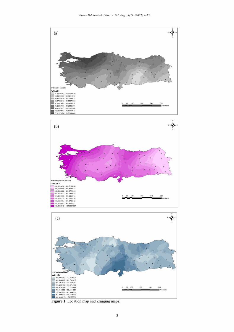
Using the "Ordinary kriging spherical model", annual

average humidity (Figure 1(a)), annual average pressure

(Figure 1(b)), annual total precipitation (Figure 1(c)),

annual average temperature (Figure 1(d)), and total

population maps (Figure 1(e)) were prepared.


3

Figure 1. Location map and krigging maps.

(c)

(a)

(b)


4

Figure 1. (Cont.) Location map and krigging maps.

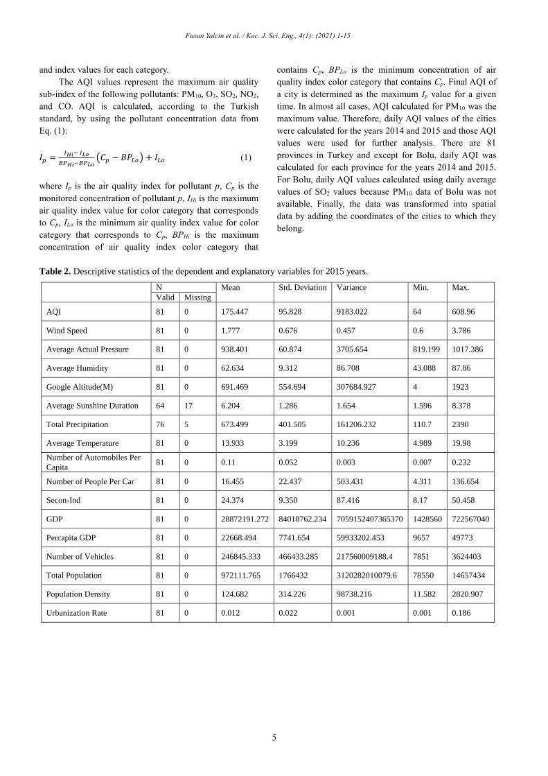
Descriptive statistics of variables for spatial models

are given in Table 2. In 2015, the lowest AQI value was

calculated in Eskişehir with 64, the highest AQI value was

608 and was calculated in Bolu. Incomplete data in the

average sunshine duration and total precipitation were

completed with the series mean method. Variation

Inflation Factor (VIF) related to linear multiple connection

problem was investigated. Accordingly, variables with

VIF> 10 are not included in the model.

2.3. Air Quality Index Calculation

The air quality data used in this study were obtained

from air quality monitoring stations operated by the

Ministry of Environment and Civilization of Turkey [28].

There was at least one air quality monitoring station in

every city that measures at least PM10 and SO2. If there

were more than one monitoring station for a city, then the

one that represents the urban background in the downtown

area was selected and used in this study.

The data coverage was from January 2014 to

December 2015. Before the use of the data, a quality

control check was done based on the correlation of data

with each other and extraordinary results were excluded

from the data set. The AQI is an index for reporting daily

air quality and its health effects by converting the observed

concentrations to a number on a range of 0 to 500. An AQI

level lower than 50 means that pollutants will not have any

significant effect to anyone. If the AQI levels are at or

higher 51, the air quality level defined as moderate, while

values below 50 considered satisfactory. Table 3 shows the

categories of AQI, the range of pollutant concentrations

(d)

(e)


5

and index values for each category.

The AQI values represent the maximum air quality

sub-index of the following pollutants: PM10, O3, SO2, NO2,

and CO. AQI is calculated, according to the Turkish

standard, by using the pollutant concentration data from

Eq. (1):

𝐼𝑝 =𝐼𝐻𝑖− 𝐼𝐿𝑜

𝐵𝑃𝐻𝑖−𝐵𝑃𝐿𝑜(𝐶𝑝 − 𝐵𝑃𝐿𝑜) + 𝐼𝐿𝑜 (1)

where Ip is the air quality index for pollutant p, Cp is the

monitored concentration of pollutant p, IHi is the maximum

air quality index value for color category that corresponds

to Cp, ILo is the minimum air quality index value for color

category that corresponds to Cp, BPHi is the maximum

concentration of air quality index color category that

contains Cp, BPLo is the minimum concentration of air

quality index color category that contains Cp. Final AQI of

a city is determined as the maximum Ip value for a given

time. In almost all cases, AQI calculated for PM10 was the

maximum value. Therefore, daily AQI values of the cities

were calculated for the years 2014 and 2015 and those AQI

values were used for further analysis. There are 81

provinces in Turkey and except for Bolu, daily AQI was

calculated for each province for the years 2014 and 2015.

For Bolu, daily AQI values calculated using daily average

values of SO2 values because PM10 data of Bolu was not

available. Finally, the data was transformed into spatial

data by adding the coordinates of the cities to which they

belong.

Table 2. Descriptive statistics of the dependent and explanatory variables for 2015 years.

N Mean Std. Deviation Variance Min. Max.

Valid Missing

AQI 81 0 175.447 95.828 9183.022 64 608.96

Wind Speed 81 0 1.777 0.676 0.457 0.6 3.786

Average Actual Pressure 81 0 938.401 60.874 3705.654 819.199 1017.386

Average Humidity 81 0 62.634 9.312 86.708 43.088 87.86

Google Altitude(M) 81 0 691.469 554.694 307684.927 4 1923

Average Sunshine Duration 64 17 6.204 1.286 1.654 1.596 8.378

Total Precipitation 76 5 673.499 401.505 161206.232 110.7 2390

Average Temperature 81 0 13.933 3.199 10.236 4.989 19.98

Number of Automobiles Per

Capita 81 0 0.11 0.052 0.003 0.007 0.232

Number of People Per Car 81 0 16.455 22.437 503.431 4.311 136.654

Secon-Ind 81 0 24.374 9.350 87.416 8.17 50.458

GDP 81 0 28872191.272 84018762.234 7059152407365370 1428560 722567040

Percapita GDP 81 0 22668.494 7741.654 59933202.453 9657 49773

Number of Vehicles 81 0 246845.333 466433.285 217560009188.4 7851 3624403

Total Population 81 0 972111.765 1766432 3120282010079.6 78550 14657434

Population Density 81 0 124.682 314.226 98738.216 11.582 2820.907

Urbanization Rate 81 0 0.012 0.022 0.001 0.001 0.186


6

Table 3. Pollutant concentrations for each AQI category of according to Turkish-AQI [28].

Index Values Category SO2 (1-hr)

(µg/m3)

NO2 (1-hr)

(µg/m3)

CO (8-hr)

(mg/m3)

O3 (8-hr)

(µg/m3)

PM10 (24-hr)

(µg/m3)

0-50 Good 0-100 0-100 0-5.5 0-120 0-50

51-100 Moderate 101-250 101-200 5.5-10 121-160 51-100

101-150 Unhealthy

for sensitive

groups

251-500 201-500 10-16 161-180 101-260

151-200 Unhealthy 501-850 501-1000 16-24 181-240 261-400

201-300 Very

unhealthy

851-1100 1001-2000 24-32 241-700 401-520

300-500 Severe >1101 >2001 >32 >701 >521

2.4. Exploratory Spatial Data Analysis

(ESDA)

Exploratory spatial data analysis (ESDA) is

frequently used in many fields of basic and social sciences.

The first studies were generally on biology and ecology,

but especially the map studies by Jhon Snow on a cholera

epidemic in London in 1854 contributed to this method

[29]. ESDA studies on air quality have been widely seen in

the literature in recent years [10], [30-33]. The phrase

"everything is related to everything else, but close things

are more related to distant things", known as Waldo

Tobler's basic law of geography, is known as the leading

sentence for spatial studies [34]. Based on this idea, we

wanted to examine whether the AQI index values are

affected by neighboring cities. The concept of spatial

dependence is similar to the autocorrelation that was

encountered in time series [35]. Therefore, spatial

dependence can be called spatial autocorrelation. Spatial

autocorrelation can offer versatile dependence, unlike the

one-way dependency in time series. Spatial dependence

shows the degree of spatial relationship between similar

units in a geographical region and error terms [36]. In this

context, there are different indices that measure spatial

dependence. The most frequently used ones can be listed

as "Moran’s I", "Geary’s C" and "General G" [37-41],

[10]. Spatial autocorrelation can be examined in two ways,

local and global. Local spatial autocorrelation (Local

Indicators of Spatial Association-LISA) has been defined

to determine the “relationship between close neighbors”.

Global spatial autocorrelation is defined to determine the

“spatial relationship of the entire region” [42-45]. In this

study, Moran's I indices, which are frequently used in the

literature, are used.

LISA, one of the spatial statistical analysis methods,

was developed with an index determined by Moran in 1948

[46]. This study was extended by Anselin in 1995 [47]. It

is used to examine the relationship between neighboring

regions. A weight matrix is created depending on the

geographical or political proximity of the neighbors. 𝑊 =

(𝑤𝑖𝑗 : 𝑖, 𝑗 = 1, … , 𝑛) is the 𝑛 𝑥 𝑛 positive matrix as Eq. (2)

[47]

[

𝑤11𝑤21

⋮𝑤𝑛1

𝑤12⋯ 𝑤1𝑛

𝑤22⋯ 𝑤2𝑛

⋮ ⋱ ⋮𝑤𝑛2

⋯ 𝑤𝑛𝑛

] (2)

The weight matrix, which is used to determine the

neighborhood, can be defined as; if 𝑖 and 𝑗 "neighbors",

then 𝑊𝑖𝑗 = 1, else 𝑊𝑖𝑗 = 0 [48]. The spatial

autocorrelation value for each region is calculated with

LISA. The GeoDa program is frequently used for the

creation of maps and for the calculation of Local Moran’s I

[47].

The local Moran’s I (LISA) used to determine local

spatial autocorrelation is as Eqs. (3-5).

𝐼𝑖 =𝑍𝑖

𝑘2∑ 𝑤𝑖𝑗𝑍𝑖𝑗 (3)

𝑘2 =∑ 𝑍𝑖

2𝑖

𝑁 (4)

𝐼 = ∑𝐼𝑖

𝑁𝑖 (5)

where, 𝐼𝑖 is the local spatial autocorrelation; 𝑁, number of

observations; 𝑍𝑖 is the deviation from the average. In other

words, Moran calculates autocorrelation by looking at the

correlation between the variable of interest and the spatial

average of that variable. Spatial average of a variable is

calculated by taking the average of that variable value in

the neighbors. The results are described in four categories;

high-high, low-low, high-low and low-high. For example,

a low-high relation indicates that once the AQI in province

A is low, the average AQI of the neighboring provinces of

province A is high. If there is also province B which shows

similar pattern around province A, than province A and B

are grouped. This indicates that these two provinces are

under the influence of same regional source or process.


7

Global spatial autocorrelation for Global Moran’s I is

calculated as Eqs. (6-7):

𝐼 =𝑛

𝑆0

∑ ∑ 𝑤𝑖𝑗(𝑥𝑖−�̅�)(𝑥𝑗−�̅�)𝑛𝑗=1

𝑛𝑖=1

∑ (𝑥𝑖−�̅�)2𝑛𝑖=1

(6)

𝑆0 = ∑ ∑ 𝑤𝑖𝑗𝑛𝑗=1

𝑛𝑖=1 (7)

where, 𝑛 is the number of cities; 𝑥𝑖 and 𝑥𝑖is the AQI of a

spatial location 𝑖, 𝑗 [49]. Global Moran indicies take values

between -1 and +1.

2.5. Spatial Models

In many similar scientific studies, the standard

approach was started by developing the non-spatial linear

regression model and then, by developing the model by

examining the spatial interaction effects of the model [50-

52]. Linear regression models are often estimated by

Ordinary Least Square (OLS). Spatial regression models,

on the other hand, are assumed to be in correlation between

each other, as opposed to traditional regression analysis

[35].

In this study, it was started with the idea that

neighboring provinces may have affected AQI values. It

was studied with the idea that independent variables may

also be affected by the neighborhood between provinces.

SLM and SEM models were used to determine these

interactions [53-54]). SEM model:

𝑌 = 𝛼𝚤𝑛 + 𝑋𝛽 + 𝜆𝑊𝑢 + 𝜀 (8)

𝜀~𝑁(0, 𝜎2𝐼𝑛)

where 𝑌 denotes an 𝑁 × 1 vector the dependent variable

for every unit in the sample (𝑖 = 1, . . . , 𝑁); 𝚤𝑁is an 𝑁 × 1

vector of ones associated with the constant term parameter

𝛼; 𝑋 denotes an 𝑁 × 𝐾 matrix of exogenous explanatory

variables; 𝛽 is a 𝐾 × 1vector of parameters; λ is the spatial

autocorrelation parameter; W denotes an 𝑁 × 𝑁 spatial

weight matrix; u is an 𝑁 × 1vector of residual and and ε is

a vector of normally distributed errors.

SLM model:

𝑌 = 𝛼𝚤𝑛 + 𝑋𝛽 + 𝜌𝑊𝑌 + 𝜀 (9)

𝜀~𝑁(0, 𝜎2𝐼𝑛)

where 𝜌 is the auto-regressive parameter [53-54],[10].

In this study, parameter estimates were obtained by

ordinary least squares Estimation (OLS) method. All

spatial regression modeling was conducted using Anselin’s

Geoda Space and Geoda software. We used ArcGIS 10.6

and Geoda to generate maps.

3. Results and Discussion

3.1. Spatial Relationship Results for AQI

In the literature, there are studies that take the AQI as

the dependent variable (i.e. the variable described). In this

study, we examined which independent variables we can

explain the AQI. We also examined whether there is a

spatial relationship in the global and local sense. Based on

this relationship, we wanted to suggest a model. Both

cluster maps and Moran I index calculations proved that

the air quality index and other variables show a spatial

distribution. The spatial distribution maps for AQI (Figure

2) showed that all the variables determined were affected

positively from neighboring provinces (i.e., the increase in

the value of one province also increased in the neighboring

province) Moran's I value was obtained as 0.279.

Figure 2. Spatial distribution of the AQI and Moran’s I

value for 2015 years.

In this study, spatial regression models were applied

instead of the traditional regression model to investigate

the relationship between the air quality index and

meteorological and anthropogenic factors. The results of

the variables showed that the independent variables

determined for the spatial regression model are in a strong

spatial relationship. These results show that AQI values are

positively affected by neighboring provinces. These results

are consistent with study in China [55].


8

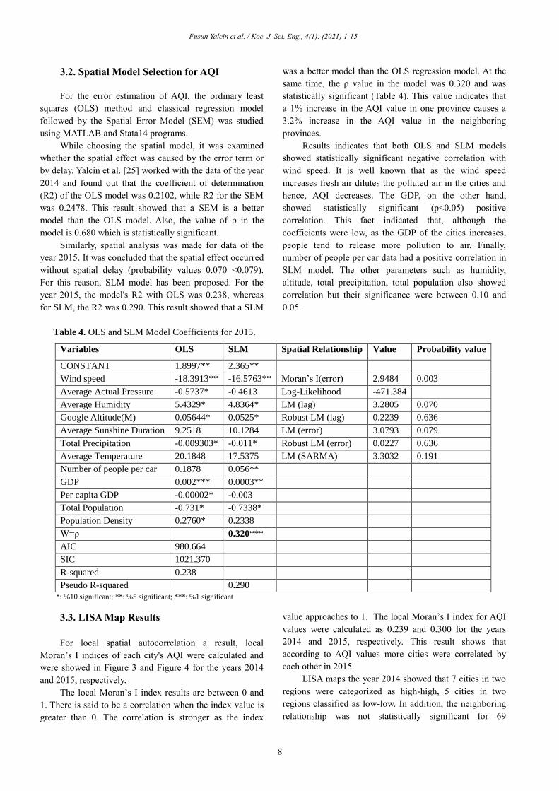
3.2. Spatial Model Selection for AQI

For the error estimation of AQI, the ordinary least

squares (OLS) method and classical regression model

followed by the Spatial Error Model (SEM) was studied

using MATLAB and Stata14 programs.

While choosing the spatial model, it was examined

whether the spatial effect was caused by the error term or

by delay. Yalcin et al. [25] worked with the data of the year

2014 and found out that the coefficient of determination

(R2) of the OLS model was 0.2102, while R2 for the SEM

was 0.2478. This result showed that a SEM is a better

model than the OLS model. Also, the value of ρ in the

model is 0.680 which is statistically significant.

Similarly, spatial analysis was made for data of the

year 2015. It was concluded that the spatial effect occurred

without spatial delay (probability values 0.070 <0.079).

For this reason, SLM model has been proposed. For the

year 2015, the model's R2 with OLS was 0.238, whereas

for SLM, the R2 was 0.290. This result showed that a SLM

was a better model than the OLS regression model. At the

same time, the ρ value in the model was 0.320 and was

statistically significant (Table 4). This value indicates that

a 1% increase in the AQI value in one province causes a

3.2% increase in the AQI value in the neighboring

provinces.

Results indicates that both OLS and SLM models

showed statistically significant negative correlation with

wind speed. It is well known that as the wind speed

increases fresh air dilutes the polluted air in the cities and

hence, AQI decreases. The GDP, on the other hand,

showed statistically significant (p<0.05) positive

correlation. This fact indicated that, although the

coefficients were low, as the GDP of the cities increases,

people tend to release more pollution to air. Finally,

number of people per car data had a positive correlation in

SLM model. The other parameters such as humidity,

altitude, total precipitation, total population also showed

correlation but their significance were between 0.10 and

0.05.

Table 4. OLS and SLM Model Coefficients for 2015.

Variables OLS SLM Spatial Relationship Value Probability value

CONSTANT 1.8997** 2.365**

Wind speed -18.3913** -16.5763** Moran’s I(error) 2.9484 0.003

Average Actual Pressure -0.5737* -0.4613 Log-Likelihood -471.384

Average Humidity 5.4329* 4.8364* LM (lag) 3.2805 0.070

Google Altitude(M) 0.05644* 0.0525* Robust LM (lag) 0.2239 0.636

Average Sunshine Duration 9.2518 10.1284 LM (error) 3.0793 0.079

Total Precipitation -0.009303* -0.011* Robust LM (error) 0.0227 0.636

Average Temperature 20.1848 17.5375 LM (SARMA) 3.3032 0.191

Number of people per car 0.1878 0.056**

GDP 0.002*** 0.0003**

Per capita GDP -0.00002* -0.003

Total Population -0.731* -0.7338*

Population Density 0.2760* 0.2338

W=ρ 0.320***

AIC 980.664

SIC 1021.370

R-squared 0.238

Pseudo R-squared 0.290

*: %10 significant; **: %5 significant; ***: %1 significant

3.3. LISA Map Results

For local spatial autocorrelation a result, local

Moran’s I indices of each city's AQI were calculated and

were showed in Figure 3 and Figure 4 for the years 2014

and 2015, respectively.

The local Moran’s I index results are between 0 and

1. There is said to be a correlation when the index value is

greater than 0. The correlation is stronger as the index

value approaches to 1. The local Moran’s I index for AQI

values were calculated as 0.239 and 0.300 for the years

2014 and 2015, respectively. This result shows that

according to AQI values more cities were correlated by

each other in 2015.

LISA maps the year 2014 showed that 7 cities in two

regions were categorized as high-high, 5 cities in two

regions classified as low-low. In addition, the neighboring

relationship was not statistically significant for 69


9

provinces. High-high relations were observed in

Zonguldak, Bolu and Düzce provinces on Black Sea region

and Mardin, Diyarbakır, Batman and Siirt provinces in

Southeastern Anatolia. AQI values for the year 2014 of

Zonguldak, Bolu and Düzce provinces, showed statistically

significant correlation (p<0.01) with Pearson correlation

coefficient varying between 0.602 (Zonguldak-Bolu) and

0.735 (Zonguldak-Düzce). The AQI of these provinces

were statistically higher than the surrounding provinces.

There are no strong natural source affecting this region.

Therefore, anthropogenic emissions, especially coal

combustion for household heating, seems to be the major

source of pollution. Similar meteorological activity in the

area could have a negative effect on accumulation of air

pollutants in the atmosphere resulting in higher AQI. In the

Southeastern Anatolia region, AQI for the year 2014 of the

four provinces (Mardin, Diyarbakır, Batman and Siirt) also

showed statistically significant correlation (p<0.01) with

Pearson correlation coefficient varying between 0.330

(Batman-Mardin) and 0.728 (Diyarbakır-Mardin). Winter

season household heating in the area is expected to be the

major local source. However, there is a very strong natural

source in the region: desert dust transport from Arabian

Peninsula [56]. The dust transport from Arabian Peninsula

seems to increase AQI values in the region.

For the both of the low-low zones observed in 2014,

the AQI values were observed lower than the surrounding

provinces. The reason of low AQI from the surrounding

provinces could be due to lower pollutant emissions than

the surrounding provinces or have a different

meteorological condition that increases the air quality of

the regions. In general, we do not expect to see lower

emissions form the surrounding provinces under same

meteorological activities, but location of the downtown

area might have an effect on such observation.

LISA maps of AQI values for 2015 showed us that.

Eight provinces in two regions were categorized as high-

high, eight provinces were grouped as low-low in one

region and two provinces were clustered as low-high. In

addition, the neighboring relationship was not statistically

significant for 63 cities. The low-low zone for the year

2015 in the Central Black Sea coast and composed of

Kırıkkale, Çorum, Kastamonu, Sinop Samsun, Ordu, Tokat

and Amasya provinces. On the east of the low-low region,

there was a low-high region consist of Bartın and

Zonguldak provinces. AQI values for the year 2015 of

these low-low and low-high classified nine provinces,



(Kırıkkale-Sinop) and 0.845 (Çorum-Tokat). The results

indicate that the meteorological conditions on the Central

Black Sea coast together with some central Anatolia region

decreases the AQI of the area. On the south of low-high

region, there was a high-high cluster. This cluster was

composed of Sakarya, Düzce and Bolu provinces. Daily

AQI values for the year 2015 of these three provinces



(Sakarya-Bolu) and 0.749 (Düzce-Bolu). These three cities

AQI values also showed statistically significant correlation

with low-low and low-high provinces located on the Black

Sea coast and Central Anatolia region (p<0.05). This

indicates that AQI show similar pattern for this group of

provinces. As indicated previously, there is not any

regional natural source in the region. The only regional

parameter is the meteorological events (precipitation and

wind speed). These parameters could vary from province

to province due to the topography of the downtown area.

Therefore, this high-high relation could be a result of local

anthropogenic emissions and similar negative effect of

meteorological events. The second high-high cluster was

on the south Anatolia and composed of Niğde, Adana, Kilis

and Osmaniye and Antakya provinces. Daily AQI values

for the year 2015 of these three provinces showed

statistically significant correlation (p<0.01) with Pearson

correlation coefficient varying between 0.439 (Niğde-

Antakya) and 0.845 (Antakya-Osmaniye). In Adana,

agriculture and agriculture related industry is dominant. In

between Adana, Antakya and Osmaniye provinces,

İskenderun Heavy Industry Zone is located. However, in

the downtown area of the other provinces, there is not any

important industrial area. Therefore, this high-high trend in

the region could not be due to local or regional

anthropogenic emissions. As indicated earlier, the South

Eastern part of Anatolia region is under influence of desert

dust transport from Arabian Peninsula. Also, studies

conducted in this region showed that desert dust transport

from Northern Africa increases the particulate matter

concentrations in the region [57-58]. Therefore, the

regional dust transport has a negative effect on AQI of

these cities.


10

Figure 3. AQI Local Moran’s I Graph and LISA Map for 2014.

Figure 4. AQI Local Moran’s I Graph and LISA Map for 2015.


11

3.3. Comparison of the AQI values of the

years 2014 and 2015

Before the comparison of the averages of 2014 and

2015 AQI values of provinces basis, normality test was

conducted. The average values of the provinces were

analyzed with the Kolmogorov-Smirnov Test and Shapiro-

Wilk test provided by the normality assumption (Table 5).

Accordingly, it was determined that the data is normally

distributed for both years.

Table 5. Tests of Normality of Annual Average AQI of

Cities for the years 2014 and 2015.

Tests of Normality

Kolmogorov-Smirnov Shapiro-Wilk

Statistic df Sig. Statistic df Sig.

Average

2014

0.075 80 0.200* 0.977 80 0.170

Average

2015

0.077 80 0.200* 0.981 80 0.275

*. This is a lower bound of the true significance.

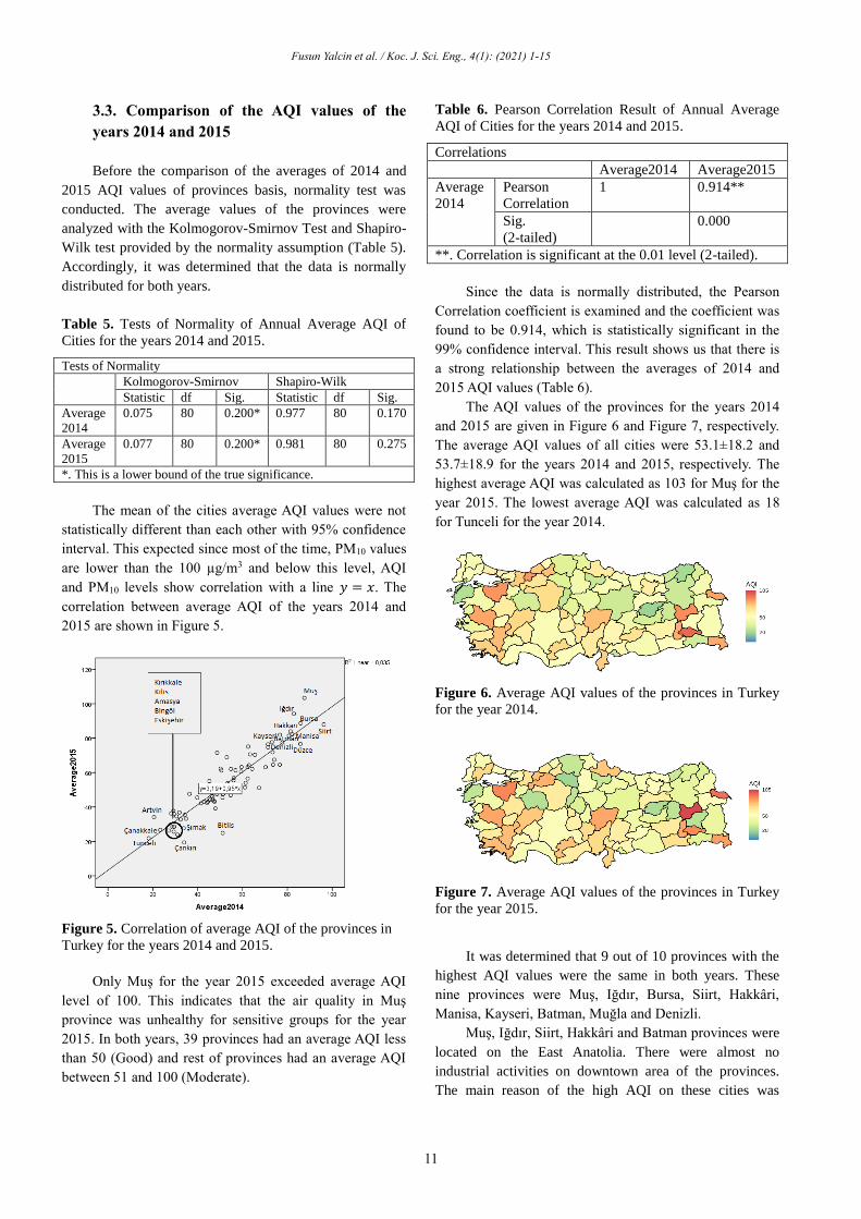
The mean of the cities average AQI values were not

statistically different than each other with 95% confidence

interval. This expected since most of the time, PM10 values

are lower than the 100 µg/m3 and below this level, AQI

and PM10 levels show correlation with a line 𝑦 = 𝑥. The

correlation between average AQI of the years 2014 and

2015 are shown in Figure 5.

Figure 5. Correlation of average AQI of the provinces in

Turkey for the years 2014 and 2015.

Only Muş for the year 2015 exceeded average AQI

level of 100. This indicates that the air quality in Muş

province was unhealthy for sensitive groups for the year

2015. In both years, 39 provinces had an average AQI less

than 50 (Good) and rest of provinces had an average AQI

between 51 and 100 (Moderate).

Table 6. Pearson Correlation Result of Annual Average

AQI of Cities for the years 2014 and 2015.

Correlations

Average2014 Average2015

Average

2014

Pearson

Correlation

1 0.914**

Sig.

(2-tailed)

0.000

**. Correlation is significant at the 0.01 level (2-tailed).

Since the data is normally distributed, the Pearson

Correlation coefficient is examined and the coefficient was

found to be 0.914, which is statistically significant in the

99% confidence interval. This result shows us that there is

a strong relationship between the averages of 2014 and

2015 AQI values (Table 6).

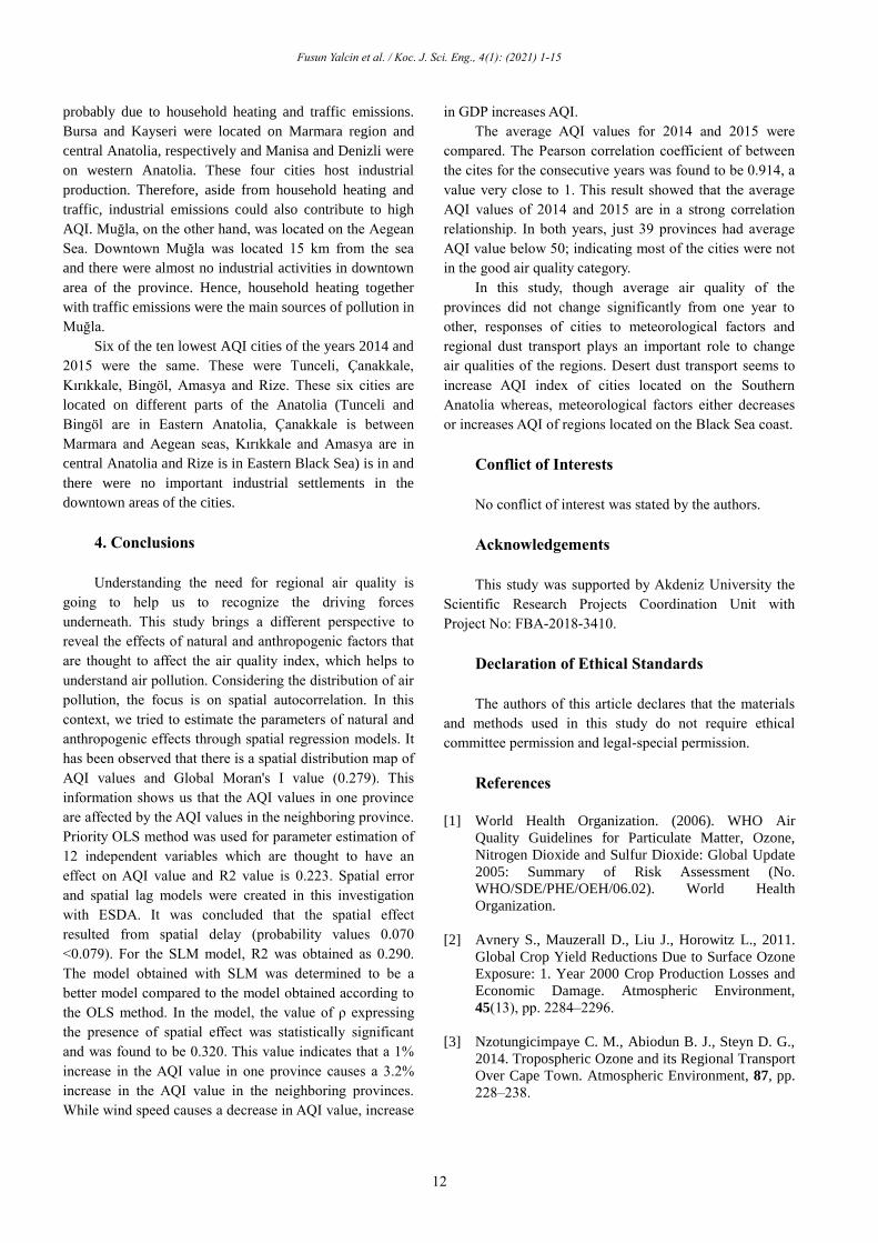
The AQI values of the provinces for the years 2014

and 2015 are given in Figure 6 and Figure 7, respectively.

The average AQI values of all cities were 53.1±18.2 and

53.7±18.9 for the years 2014 and 2015, respectively. The

highest average AQI was calculated as 103 for Muş for the

year 2015. The lowest average AQI was calculated as 18

for Tunceli for the year 2014.

Figure 6. Average AQI values of the provinces in Turkey

for the year 2014.

Figure 7. Average AQI values of the provinces in Turkey

for the year 2015.

It was determined that 9 out of 10 provinces with the

highest AQI values were the same in both years. These

nine provinces were Muş, Iğdır, Bursa, Siirt, Hakkâri,

Manisa, Kayseri, Batman, Muğla and Denizli.

Muş, Iğdır, Siirt, Hakkâri and Batman provinces were

located on the East Anatolia. There were almost no

industrial activities on downtown area of the provinces.

The main reason of the high AQI on these cities was


12

probably due to household heating and traffic emissions.

Bursa and Kayseri were located on Marmara region and

central Anatolia, respectively and Manisa and Denizli were

on western Anatolia. These four cities host industrial

production. Therefore, aside from household heating and

traffic, industrial emissions could also contribute to high

AQI. Muğla, on the other hand, was located on the Aegean

Sea. Downtown Muğla was located 15 km from the sea

and there were almost no industrial activities in downtown

area of the province. Hence, household heating together

with traffic emissions were the main sources of pollution in

Muğla.

Six of the ten lowest AQI cities of the years 2014 and

2015 were the same. These were Tunceli, Çanakkale,

Kırıkkale, Bingöl, Amasya and Rize. These six cities are

located on different parts of the Anatolia (Tunceli and

Bingöl are in Eastern Anatolia, Çanakkale is between

Marmara and Aegean seas, Kırıkkale and Amasya are in

central Anatolia and Rize is in Eastern Black Sea) is in and

there were no important industrial settlements in the

downtown areas of the cities.

4. Conclusions

Understanding the need for regional air quality is

going to help us to recognize the driving forces

underneath. This study brings a different perspective to

reveal the effects of natural and anthropogenic factors that

are thought to affect the air quality index, which helps to

understand air pollution. Considering the distribution of air

pollution, the focus is on spatial autocorrelation. In this

context, we tried to estimate the parameters of natural and

anthropogenic effects through spatial regression models. It

has been observed that there is a spatial distribution map of

AQI values and Global Moran's I value (0.279). This

information shows us that the AQI values in one province

are affected by the AQI values in the neighboring province.

Priority OLS method was used for parameter estimation of

12 independent variables which are thought to have an

effect on AQI value and R2 value is 0.223. Spatial error

and spatial lag models were created in this investigation

with ESDA. It was concluded that the spatial effect

resulted from spatial delay (probability values 0.070

<0.079). For the SLM model, R2 was obtained as 0.290.

The model obtained with SLM was determined to be a

better model compared to the model obtained according to

the OLS method. In the model, the value of ρ expressing

the presence of spatial effect was statistically significant

and was found to be 0.320. This value indicates that a 1%

increase in the AQI value in one province causes a 3.2%

increase in the AQI value in the neighboring provinces.

While wind speed causes a decrease in AQI value, increase

in GDP increases AQI.

The average AQI values for 2014 and 2015 were

compared. The Pearson correlation coefficient of between

the cites for the consecutive years was found to be 0.914, a

value very close to 1. This result showed that the average

AQI values of 2014 and 2015 are in a strong correlation

relationship. In both years, just 39 provinces had average

AQI value below 50; indicating most of the cities were not

in the good air quality category.

In this study, though average air quality of the

provinces did not change significantly from one year to

other, responses of cities to meteorological factors and

regional dust transport plays an important role to change

air qualities of the regions. Desert dust transport seems to

increase AQI index of cities located on the Southern

Anatolia whereas, meteorological factors either decreases

or increases AQI of regions located on the Black Sea coast.

Conflict of Interests

No conflict of interest was stated by the authors.

Acknowledgements

This study was supported by Akdeniz University the

Scientific Research Projects Coordination Unit with

Project No: FBA-2018-3410.

Declaration of Ethical Standards

The authors of this article declares that the materials

and methods used in this study do not require ethical

committee permission and legal-special permission.

References

[1] World Health Organization. (2006). WHO Air

Quality Guidelines for Particulate Matter, Ozone,

Nitrogen Dioxide and Sulfur Dioxide: Global Update

2005: Summary of Risk Assessment (No.

WHO/SDE/PHE/OEH/06.02). World Health

Organization.

[2] Avnery S., Mauzerall D., Liu J., Horowitz L., 2011.

Global Crop Yield Reductions Due to Surface Ozone

Exposure: 1. Year 2000 Crop Production Losses and

Economic Damage. Atmospheric Environment,

45(13), pp. 2284‒2296.

[3] Nzotungicimpaye C. M., Abiodun B. J., Steyn D. G.,

2014. Tropospheric Ozone and its Regional Transport

Over Cape Town. Atmospheric Environment, 87, pp.

228‒238.


13

[4] Dimitriou K., Kassomenos P., 2015. Three Year

Study of Tropospheric Ozone with Back Trajectories

at A Metropolitan and A Medium Scale Urban Area

in Greece. Science of the Total Environment, 502, pp.

493‒501.

[5] Cape J.N., Fowler D., Davison A., 2003. Ecological

Effects of Sulfur Dioxide, Fluorides, and Minor Air

Pollutants: Recent Trends and Research Needs.

Environment International, 29(2), pp. 201‒211.

[6] EPA, 2014. Air Quality Index: A Guide to Air

Quality and Your Health. NC, USA.

[7] Lee E., Chan C.K., Paatero P., 1999. Application of

Positive Matrix Factorization in Source

Apportionment of Particulate Pollutants in Hong

Kong. Atmospheric Environment, 33(19). pp. 3201‒

3212.

[8] Querol X., Alastuey A., Rodriguez S., Plana F., Ruiz

C.R., Cots N., Massagué G., Puig O., 2001. PM10 and

PM2.5 Source Apportionment in the Barcelona

Metropolitan Area, Catalonia, Spain. Atmospheric

Environment, 35(36), pp. 6407-6419.

[9] Mansha M., Ghauri B., Rahman S. Amman A. 2012.

Characterization and Source Apportionment of

Ambient Air Particulate Matter (PM2.5) in Karachi.

Science Of The Total Environment, 425, pp. 176-183.

[10] Liu H., Fang C., Zhang X., Wang Z., Bao C., Li F.,

2017. The Effect of Natural and Anthropogenic

Factors on Haze Pollution in Chinese Cities: A

Spatial Econometrics Approach. Journal of Cleaner

Prod., 165, pp. 323-333.

[11] Xu W., Tian Y., Liu Y., Zhao B., Liu Y., Zhang X.

2019. Understanding the Spatial-Temporal Patterns

and Influential Factors on Air Quality Index: The

Case of North China. International Journal of

Environmental Research and Public Health, 16(16),

pp. 2820.

[12] Gaga E. O., Döğeroğlu T., Özden Ö., Ari A., Yay O.

D., Altuğ H., Van Doorn, W., 2012. Evaluation of Air

Quality by Passive and Active Sampling in An Urban

City in Turkey: Current Status and Spatial Analysis

of Air Pollution Exposure. Environmental Science

and Pollution Research, 19(8), pp. 3579-3596.

[13] Demir M., Dindaroğlu T., Yılmaz S., 2014. Effects of

Forest Areas on air Quality; Aras Basin and its

Environment. Journal of Environmental Health

Science and Engineering, 12(1), pp. 60.

[14] Tecer L. H., Tagil S., 2014. Impact of Urbanization

on Local Air Quality: Differences in Urban and Rural

Areas of Balikesir, Turkey. CLEAN–Soil, Air, Water,

42(11), pp.1489-1499.

[15] Dursun S., Alqaysi N. H. H., 2016. Estimating Air

Pollution Quality In Istanbul City Centre By

Geographic Information System. International

Journal Of Ecosystems And Ecology Science-IjeeS,

6(3), pp. 329-340.

[16] Kurnaz K., Cobanoglu G., 2017. Biomonitoring of

Air Quality in Istanbul Metropolitan Territory with

Epiphytic Lichen Physcia Adscendens (Fr.) Olivier.

Fresen. Environ. Bull, 26, pp. 7296.

[17] Baykara M., Im U., Unal A., 2019. Evaluation of

Impact of Residential Heating on Air Quality of

Megacity Istanbul by CMAQ. Science of the Total

Environment, 651, pp.1688-1697.

[18] Güçlü Y. S., Dabanlı İ., Şişman E., Şen, Z., 2019. Air

Quality (AQ) Identification by Innovative Trend

Diagram and AQ Index Combinations in Istanbul

Megacity. Atmospheric Pollution Research, 10(1),

pp. 88-96.

[19] Gokce H. B., Arıoğlu E., Copty N. K., Onay T. T.,

Gun B., 2020. Exterior Air Quality Monitoring for

The Eurasia Tunnel in Istanbul, Turkey. Science of

The Total Environment, 699, pp. 134312.

[20] Dagsuyu C., 2020. Process Capability and Risk

Assessment for Air Quality: an Integrated Approach.

Human and Ecological Risk Assessment: An

International Journal, 26(2), pp. 394-405.

[21] Yalcin F., 2016, “Spatial Analysis of The Factors

Affecting The Room Price Offered by The Hotels in

Antalya City” (in Turkish), Unpublished Doctorate

Thesis, Akdeniz University, Graduate School of

Social Sciences, Antalya, Turkey.

[22] Yalcin F., Mert M., 2018. Determinación de Precios

Hedónicos de Habitación de Hotel con Efecto

Espacial en Antalya. Economía, Sociedad y territorio,

18(58), pp.697-734.

[23] Kowe P., Mutanga O., Odindi J., Dube T., 2019.

Exploring the Spatial Patterns of Vegetation

Fragmentation Using Local Spatial Autocorrelation

Indices. Journal of Applied Remote Sensing, 13(2),

pp. 1-14.

[24] Lutz S.U., 2019. The European Digital Single Market

Strategy: Local Indicators of Spatial Association

2011–2016. Telecommunications Policy, 43(5), pp.

393-410.

[25] Yalcin F., Tepe A., Dogan G., Cizmeci N., 2019.

Investigation of Air Quality Index by Spatial Data

Analysis: a Case Study on Turkey. Proceedings Book

of the 2nd Mediterranean, 23.


14

[26] Sensoy S., Demircan M., Ulupinar Y., Balta I., 2008.

Climate of Turkey. Turkish State Meteorological

Service, 401.

[27] Yalcin F., Tepe A. M., Doğan G., Cizmeci N. 2019.

Regression Analysis of The Effect of Meteorological

Parameters on Air Quality in Three Neighboring

Cities Located on The Mediterranean Coast of

Turkey. In AIP Conference Proceedings, July, Vol.

2116, No. 1, p. 100015. AIP Publishing LLC.

[28] CSB. 2020. SIM Veri Bankasi. (Web page:

https://sim.csb.gov.tr) (Date accessed: 01.04.2020).

[29] Snow J., 1855. On the Mode of Communication of

Cholera (2nd ed.). London: John Churchill.

[30] Fang C., Liu H., Li G., Sun D., Miao Z., 2015.

Estimating the Impact of Urbanization on Air Quality

in China Using Spatial Regression Models.

Sustainability, 7(11), pp. 15570-15592.

[31] Mahara G., Wang C., Yang K., Chen S., Guo J., Gao

Q., Guo, X., 2016. The Association Between

Environmental Factors and Scarlet Fever Incidence in

Beijing Region: Using GIS and Spatial Regression

Models. International Journal of Environmental

Research and Public Health, 13(11), pp.1083.

[32] Guo Y., Tang Q., Gong D. Y., Zhang Z., 2017.

Estimating Ground-Level PM2. 5 Concentrations in

Beijing Using a Satellite-Based Geographically and

Temporally Weighted Regression Model.Remote

Sensing of Environment, 198, pp. 140-149.

[33] Li H., You S., Zhang H., Zheng W., Zheng X., Jia J.,

Zou L., 2017. Modelling of AQI Related to Building

Space Heating Energy Demand Based on Big Data

Analytics. Applied Energy, 203, pp. 57-71.

[34] Tobler W. R., 1970. A Computer Movie Simulating

Urban Growth in The Detroit Region. Economic

Geography, 46(sup1), pp. 234-240.

[35] Anselin L., 1988. Spatial Econometrics: Methods

And Models, Kluwer Academic Publishers,

Dordrecht.

[36] Cliff A. D., Ord J. K., Haggett P., Versey G. R.,

1981.Spatial Diffusion: An Historical Geography of

Epidemics in an island community (Vol. 14). CUP

Archive.

[37] Moran P.A.P., 1950a. Notes on Continuous

Stochastic Phenomena. Biometrika, 37, pp.17-23.

[38] Moran P.A.P., 1950b. A Test for The Serial

Independence of Residuals. Biometrika, 37, pp. 178-

181.

[39] Geary R. C., 1954. The Contiguity Ratio and

Statistical Mapping. The Incorporated Statistician,

5(3), pp. 115-146.

[40] Getis A., 2008. A History of The Concept of Spatial

Autocorrelation: A Geographer's Perspective.

Geographical Analysis, 40(3), pp. 297-309.

[41] Wheeler D.C., Tiefelsdorf M., 2005. Multicollinearity

and Correlation Among Local Regression

Coefficients in Geographically Weighted Regression.

Journal of Geographical Systems 7, pp. 161–87.

[42] Ord J. K., Getis A., 1995. Local Spatial

Autocorrelation Statistics: Distributional Issues and

an Application.Geographical Analysis, 27(4), pp.

286-306.

[43] Anselin L., Bera A. K., Florax R., Yoon M. J., 1996.

Simple Diagnostic Tests for Spatial Dependence.

Regional Science and Urban Economics, 26(1), pp.

77-104.

[44] Getis A., Ord J. K., 1996. Spatial Analysis and

Modeling in A GIS Environment. A research Agenda

for Geographic Information Science, pp.157-196.

[45] Boots B., Tiefelsdorf M., 2000. Global and Local

Spatial Autocorrelation in Bounded Regular

Tessellations. Journal of Geographical Systems, 2(4),

pp. 319-348.

[46] Moran P.A.P., 1948. The Interpretation of Statistical

Maps. Journal of the Royal Statistical Society B., 10,

pp. 243-251

[47] Anselin L., 1995. Local Indicators of Spatial

Association-LISA, Geographical Analysis, 27, pp.

93-115.

[48] Anselin L., Florax, R.J.G.M., Rey, S.J. (ed.). 2004.

Advances in Spatial Econometrics, Methodology,

Tools and Applications. Springer-Verlag Berlin

Heidelberg, Berlin.

[49] Anselin L., Hudak S., 1992. Spatial Econometrics in

Practice: A Review of Software Options. Regional

Science and Urban Economics, 22(3), pp.509-536.

[50] Li X. X., Wang L. X., Zhang J., Liu Y. X., Zhang H.,

Jiang S. W., Zhou X. N., 2014. Exploration of

Ecological Factors Related to The Spatial

Heterogeneity of Tuberculosis Prevalence in PR

China. Global Health Action, 7(1), pp.23620.

[51] Jung M. C., Park J., & Kim S., 2019. Spatial

Relationships Between Urban Structures and Air

Pollution in Korea. Sustainability, 11(2), p. 476.


15

[52] Wang M., Wang H., 2020. Spatial Distribution

Patterns and Influencing Factors of PM 2.5 Pollution

in the Yangtze River Delta: Empirical Analysis Based

on a GWR Model. Asia-Pacific Journal of

Atmospheric Sciences, pp.1-13.

[53] Anselin L., 2013. Spatial Econometrics: Methods and

Models (Vol. 4). Springer Science & Business Media.

[54] Elhorst J. P., 2010. Applied Spatial Econometrics:

Raising the Bar. Spatial Economic Analysis, 5(1), pp.

9-28.

[55] Liu, H., Fang, C., Zhang, X., Wang, Z., Bao, C., Li

F., 2017. The Effect of Natural and Anthropogenic

Factors on Haze Pollution in Chinese Cities: A

Spatial Econometrics Approach. Journal of Cleaner

Prod., 165, pp. 323-333

[56] Ecer A., Sarikaya B., Tepe A. M., Doğan, G., 2017.

Mardin Ili Hava Kalitesinin Degerlendirilmesi. Paper

Presented at the 7. Ulusal Hava Kirliliği ve Kontrolü

Sempozyumu, Antalya, Turkey.

[57] Tepe A. M., Doğan G., 2016. Comparison of Effect

of Saharan Dust Transport to Cities Located on Black

Sea and Mediterranean Coasts of Turkey. Paper

Presented at the 1st International Black Sea Congress

on Environmental Sciences, Giresun, Turkey.

[58] Tepe A. M., Doğan G., 2019. Türkiye'nin Güney

Sahilinde Yer Alan Dört Sehrin Have Kalitelerinin

Incelenmesi. Mühendislik Bilimleri ve Tasarım

Dergisi, 7(3) , pp. 585-595.

Documents

Kocaeli Journal of Science and Engineering Spatial