Embed Size (px)
Citation preview
8/3/2019 Ko Honda, William H. Kazez and Gordana Matic- The Contact Invariant in Sutured Floer Homology
http://slidepdf.com/reader/full/ko-honda-william-h-kazez-and-gordana-matic-the-contact-invariant-in-sutured 1/34
a r X i v : 0 7 0 5
. 2 8 2 8 v 2
[ m a t h . G T
] 2 1 O c t 2 0 0 7
THE CONTACT INVARIANT IN SUTURED FLOER HOMOLOGY
KO HONDA, WILLIAM H. KAZEZ, AND GORDANA MATIC
Abstract. We describe an invariant of a contact 3-manifold with convex boundary as anelement of Juhasz’s sutured Floer homology. Our invariant generalizes the contact invariantin Heegaard Floer homology in the closed case, due to Ozsvath and Szabo.
The goal of this paper is to present an invariant of a contact 3-manifold with convexboundary. The contact class is an element of sutured Floer homology , defined by Andras
Juhasz, and generalizes the contact class in Heegaard Floer homology in the closed case,as defined by Ozsvath and Szabo [OS3] and reformulated by the authors in [HKM2]. Inthis paper we assume familiarity with convex surface theory (cf. [Gi1, H1]), Heegaard Floerhomology (cf. [OS1, OS2]), and sutured manifold theory (cf. [Ga]).
Sutured manifold theory was introduced by Gabai [Ga] to study and construct taut fo-liations. A sutured manifold (M, Γ) is a compact oriented 3-manifold (not necessarily con-nected) with boundary, together with a compact subsurface Γ = A(Γ) ⊔ T (Γ) ⊂ ∂M , whereA(Γ) is a union of pairwise disjoint annuli and T (Γ) is a union of tori. We orient eachcomponent of ∂M − Γ, subject to the condition that the orientation changes every time wenontrivially cross A(Γ). Let R+(Γ) (resp. R−(Γ)) be the open subsurface of ∂M − Γ onwhich the orientation agrees with (resp. is the opposite of) the boundary orientation on ∂M .
Moreover, Γ is oriented so that the orientation agrees with the orientation of ∂R+(Γ) and isthe opposite that of ∂R−(Γ). A sutured manifold (M, Γ) is balanced if M has no closed com-ponents, π0(A(Γ)) → π0(∂M ) is surjective, and χ(R+(Γ)) = χ(R−(Γ)) on every componentof M . In particular, Γ = A(Γ) and every boundary component of ∂M nontrivially intersectsthe suture Γ. In this paper, all our sutured manifolds are assumed to be balanced.
In what follows, we view the suture Γ as the union of cores of the annuli, i.e., as a disjointunion of simple closed curves.
In the setting of contact structures, a natural condition to impose on a contact 3-manifold(M, ξ) with boundary is to require that ∂M be convex , i.e., there is a contact vector fieldtransverse to ∂M . To a convex surface F one can associate its dividing set ΓF — it is definedas the isotopy class of multicurves {x ∈ F |X (x) ∈ ξ(x)}, where X is a transverse contact
vector field. It was explained in [HKM3] that dividing sets and sutures on balanced suturedmanifolds can be viewed as equivalent objects. As usual, our contact structures are assumedto be cooriented.
Date: This version: September 10, 2007. (The pictures are in color.)1991 Mathematics Subject Classification. Primary 57M50; Secondary 53C15.Key words and phrases. tight, contact structure, open book decomposition, fibered link, Dehn twists,
Heegaard Floer homology, sutured manifolds.KH supported by an NSF CAREER Award (DMS-0237386); GM supported by NSF grant DMS-0410066;
WHK supported by NSF grant DMS-0406158.1
8/3/2019 Ko Honda, William H. Kazez and Gordana Matic- The Contact Invariant in Sutured Floer Homology
http://slidepdf.com/reader/full/ko-honda-william-h-kazez-and-gordana-matic-the-contact-invariant-in-sutured 2/34
2 KO HONDA, WILLIAM H. KAZEZ, AND GORDANA MATIC
In a pair of important papers [Ju1, Ju2], Andras Juhasz generalized (the hat versions of)Ozsvath and Szabo’s Heegaard Floer homology [OS1, OS2] and link Floer homology [OS4]
theories, and assigned a Floer homology group SFH (M, Γ) to a balanced sutured manifold(M, Γ). (A similar theory was also worked out by Lipshitz [Li2].) An important property
of this sutured Floer homology is the following: if (M, Γ)T (M ′, Γ′) is a sutured mani-
fold decomposition along a cutting surface T , then SFH (M ′, Γ′) is a direct summand of SFH (M, Γ).
The main result of this paper is the following:
Theorem 0.1. Let (M, Γ) be a balanced sutured manifold, and let ξ be a contact structureon M with convex boundary, whose dividing set on ∂M is Γ. Then there exists an invariant EH (M, Γ, ξ) of the contact structure which lives in SFH (−M, −Γ)/{±1}.
Here we are using Z-coefficients. Note that there is currently a ±1 ambiguity when Z-
coefficients are used.The paper is organized as follows. Section 1 is devoted to discussing the contact-topological
preliminaries for obtaining a partial open book decomposition of a contact 3-manifold withconvex boundary. We define the contact invariant in Section 2 and prove that it is indepen-dent of the choices made in Section 3. We discuss some basic properties of the contact classin Section 4 and compute some examples in Section 5. Finally, we explain the relationshipto sutured manifold decompositions in Section 6.
1. Contact structure preliminaries
Let (M, Γ) be a sutured manifold. Let ξ be a contact structure on M with convex boundary
so that the dividing set Γ∂M on ∂M is isotopic to Γ. Such a contact manifold will be denoted(M, Γ, ξ).The following theorem is the key to obtaining a partial open book decomposition, slightly
generalizing the work of Giroux [Gi2] to the relative case. For more detailed expositions of Giroux’s work, see [Co2, Et].
Theorem 1.1. There exists a Legendrian graph K ⊂ M whose endpoints, i.e., univalent vertices, lie on Γ ⊂ ∂M and which satisfies the following:
(1) There is a neighborhood N (K ) ⊂ M of K so that (i) ∂N (K ) = T ∪ (∪iDi), (ii) T is a convex surface with Legendrian boundary, (iii) Di ⊂ ∂M is a convex disk with Legendrian boundary, (iv) T ∩ ∂M = ∪i∂Di, (v) #(∂Di ∩ Γ∂M ) = 2, and (vi) thereis a system of pairwise disjoint compressing disks D′
jfor N (K ) so that ∂D ′
j⊂ T ,
|∂D ′ j ∩ ΓT | = 2, and each component of N (K ) − ∪ jD′
j is a standard contact 3-ball,after rounding the corners.
(2) Each component H of the complement M −N (K ) is a handlebody with convex bound-ary. There is a system of pairwise disjoint compressing disks Dα
k for H so that |∂Dα
k ∩ Γ∂H | = 2 and H − ∪kDαk is a standard contact 3-ball, after rounding the
corners.
Here | · | denotes the geometric intersection number and #(·) denotes the number of connected components. A standard contact 3-ball is a tight contact 3-ball B3 with convex
8/3/2019 Ko Honda, William H. Kazez and Gordana Matic- The Contact Invariant in Sutured Floer Homology
http://slidepdf.com/reader/full/ko-honda-william-h-kazez-and-gordana-matic-the-contact-invariant-in-sutured 3/34
THE CONTACT INVARIANT IN SUTURED FLOER HOMOLOGY 3
boundary and #Γ∂B3 = 1. We say that a handlebody H with convex boundary admits aproduct disk decomposition if condition (2) of Theorem 1.1 holds.
Proof. Since F = ∂M is convex, there is an I = [0, 1]-invariant contact neighborhood F ×I ⊂M so that F × {1} = ∂M . First we take a polyhedral decomposition of F 0 = F × {0} so thatthe 1-skeleton is Legendrian and the boundary of each 2-cell intersects ΓF 0 in two points.During this process we need to use the Legendrian realization principle and slightly isotopF 0. Next, extend the polyhedral decomposition on F 0 to M − (F × I ) so that the 1-skeletonK ′ is Legendrian and the boundary of each 2-cell has Thurston-Bennequin invariant tb = −1.Finally, we need to connect K ′ to ∂M . To achieve this, for each intersection point p of K ′|F 0
with ΓF 0 , we add an edge { p} × [0, 1] ⊂ F × [0, 1] to K ′. The resulting graph is our desiredK .
We now prove that K satisfies the properties of the theorem. There is a collection of compressing disks in (M − N (K ′)) − (F × I ) which intersect the dividing set Γ
∂N (K ′
)at
exactly two points, by the tb = −1 condition. Without loss of generality, these compressingdisks can be made convex with Legendrian boundary. Then the compressing disks cut up M −N (K ′) into a disjoint union of standard contact 3-balls and F × I . After removing standardneighborhoods of { p} × I from F × I , the remaining contact 3-manifold admits a productdisk decomposition. This implies that M − N (K ) admits a product disk decomposition.
The next theorem is the relative version of the subdivision theorem of Giroux [Gi2] for con-tact cellular decompositions, which implies that on a closed manifold M any two open bookscorresponding to a fixed (M, ξ) become isotopic after a sequence of positive stabilizations toeach.
Theorem 1.2. Let K and K ′
be Legendrian graphs on (M, Γ, ξ) which satisfy the conditionsof Theorem 1.1 and K ∩ K ′ = ∅. Then there exists a common Legendrian extension L of K and K ′ so that L = K n is obtained inductively from K = K 0 by attaching Legendrian arcsci, i = 1, . . . , n − 1, to the standard neighborhood N (K i) of K i so that the following hold:
(1) The arc ci has both endpoints on the dividing set of ∂ (M − N (K i)), and int(ci) ⊂int(M − N (K i)).
(2) N (K i+1) = N (ci) ∪ N (K i), and K i+1 is a Legendrian graph so that N (K i+1) is itsstandard neighborhood.
(3) There is a Legendrian arc di on ∂ (M − N (K i)) with the same endpoints as ci, after possible application of the Legendrian realization principle. The arc di intersectsΓ∂ (M −N (K i)) only at its endpoints.
(4) The Legendrian knot γ i = ci ∪ di bounds a disk in M − N (K i) and has tb(γ i) = −1with respect to this disk. This implies that ci and di are Legendrian isotopic relativeto their endpoints inside the closure of M − N (K i).
The graph L = K ′m is similarly obtained from K ′ = K ′0 by inductively attaching Legendrian arcs c′i to N (K ′i) to obtain K ′i+1.
Proof. Consider the invariant neighborhood F × [0, 1] with F = F 1 = ∂M as in the firstparagraph of Theorem 1.1, and take a copy F 1−δ near F . The procedure for finding acommon refinement L of K and K ′ is as follows:
8/3/2019 Ko Honda, William H. Kazez and Gordana Matic- The Contact Invariant in Sutured Floer Homology
http://slidepdf.com/reader/full/ko-honda-william-h-kazez-and-gordana-matic-the-contact-invariant-in-sutured 4/34
4 KO HONDA, WILLIAM H. KAZEZ, AND GORDANA MATIC
(1) First add Legendrian arcs to K so that K i, i ≫ 0, contains a Legendrian 1-skeletonof the protective layer F 1−δ (as in the first paragraph of Theorem 1.1).
(2) Subdivide the Legendrian 1-skeleton of F 1−δ sufficiently, so that every arc of K ′
near∂M (we assume they are all of the form { p} × [1 − δ, 1]) intersects the 1-skeleton.(3) Next add enough Legendrian arcs of the type { p} × [1 − δ, 1], where p ∈ ΓF , so that
K i ⊃ (K ∪ K ′) ∩ (F × [1 − δ, 1]), i ≫ 0.(4) Finally, apply the contact subdivision procedure of [Gi2] away from F × [1 − δ, 1].
Steps (2) and (4) involve the same procedure used in [Gi2], namely, given a face ∆ of thecontact cellular decomposition with Legendrian boundary ∂ ∆ ⊂ K , take a Legendrian arcci ⊂ ∆ with endpoints on ∂ ∆, so that ci cuts ∆ into ∆1, ∆2, each of which has tb(∂ ∆i) = −1.
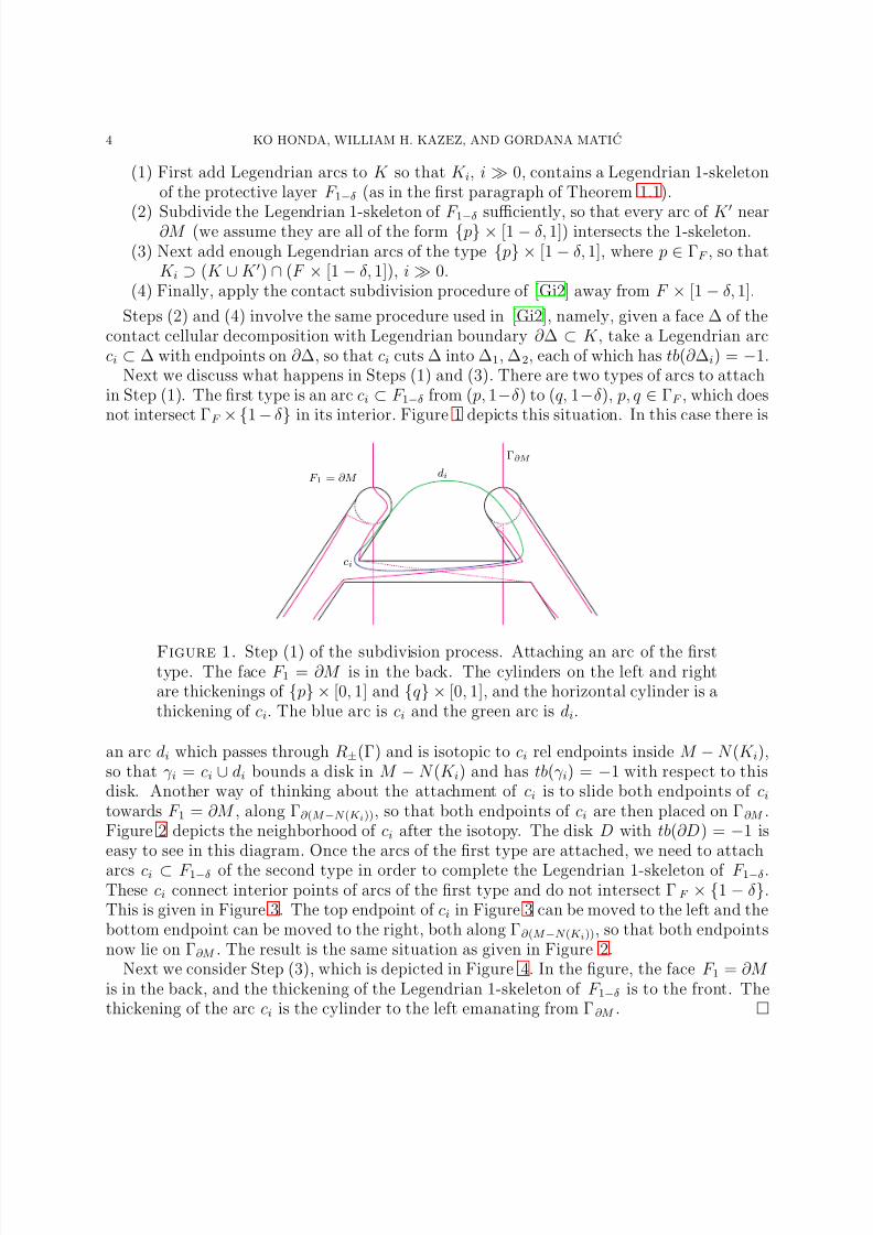
Next we discuss what happens in Steps (1) and (3). There are two types of arcs to attachin Step (1). The first type is an arc ci ⊂ F 1−δ from ( p, 1−δ) to (q, 1−δ), p, q ∈ ΓF , which doesnot intersect ΓF × {1 − δ} in its interior. Figure 1 depicts this situation. In this case there is
F 1 = ∂M
Γ∂M
di
ci
Figure 1. Step (1) of the subdivision process. Attaching an arc of the firsttype. The face F 1 = ∂M is in the back. The cylinders on the left and rightare thickenings of { p} × [0, 1] and {q} × [0, 1], and the horizontal cylinder is athickening of ci. The blue arc is ci and the green arc is di.
an arc di which passes through R±(Γ) and is isotopic to ci rel endpoints inside M − N (K i),so that γ i = ci ∪ di bounds a disk in M − N (K i) and has tb(γ i) = −1 with respect to thisdisk. Another way of thinking about the attachment of ci is to slide both endpoints of ci
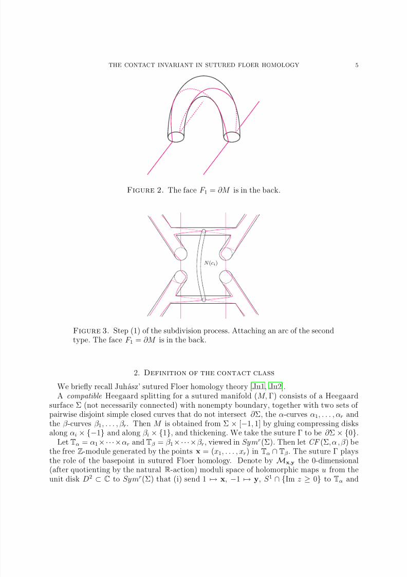
towards F 1 = ∂M , along Γ∂ (M −N (K i)), so that both endpoints of ci are then placed on Γ∂M .Figure 2 depicts the neighborhood of ci after the isotopy. The disk D with tb(∂D) = −1 iseasy to see in this diagram. Once the arcs of the first type are attached, we need to attach
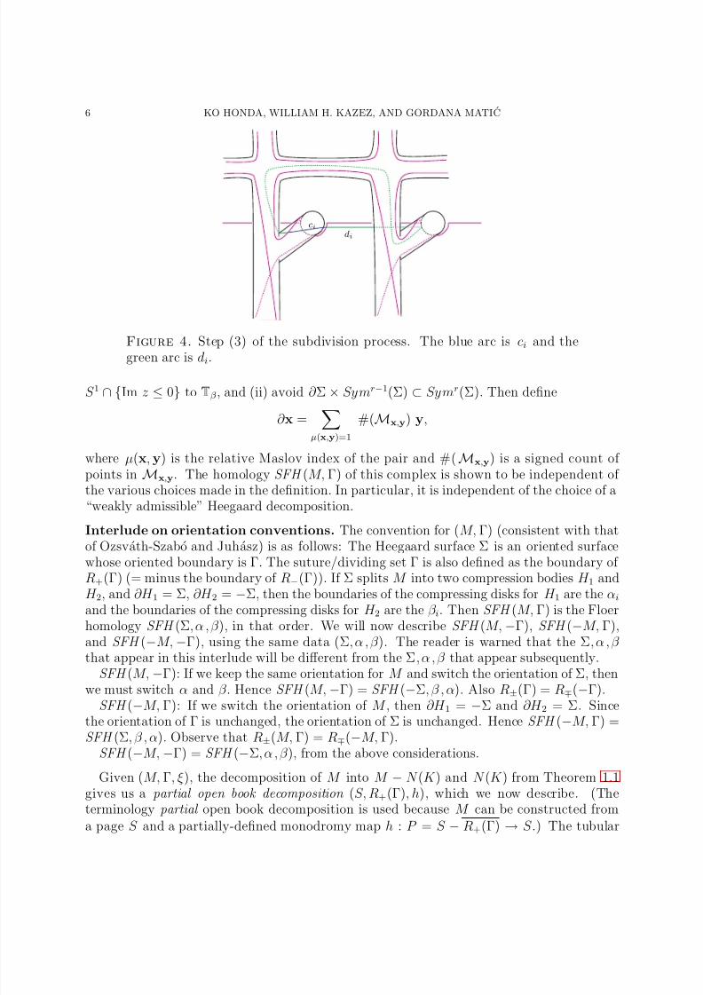
arcs ci ⊂ F 1−δ of the second type in order to complete the Legendrian 1-skeleton of F 1−δ.These ci connect interior points of arcs of the first type and do not intersect ΓF × {1 − δ}.This is given in Figure 3. The top endpoint of ci in Figure 3 can be moved to the left and thebottom endpoint can be moved to the right, both along Γ∂ (M −N (K i)), so that both endpointsnow lie on Γ∂M . The result is the same situation as given in Figure 2.
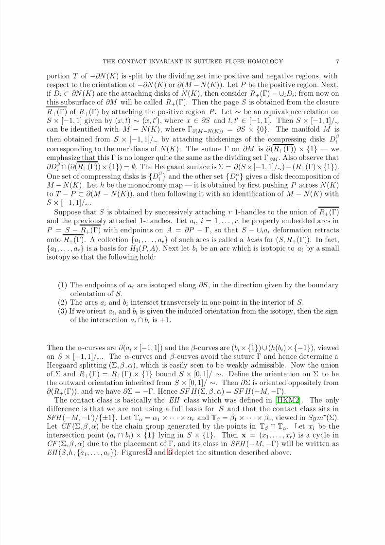
Next we consider Step (3), which is depicted in Figure 4. In the figure, the face F 1 = ∂M is in the back, and the thickening of the Legendrian 1-skeleton of F 1−δ is to the front. Thethickening of the arc ci is the cylinder to the left emanating from Γ∂M .
8/3/2019 Ko Honda, William H. Kazez and Gordana Matic- The Contact Invariant in Sutured Floer Homology
http://slidepdf.com/reader/full/ko-honda-william-h-kazez-and-gordana-matic-the-contact-invariant-in-sutured 5/34
THE CONTACT INVARIANT IN SUTURED FLOER HOMOLOGY 5
Figure 2. The face F 1 = ∂M is in the back.
N (ci)
Figure 3. Step (1) of the subdivision process. Attaching an arc of the secondtype. The face F 1 = ∂M is in the back.
2. Definition of the contact class
We briefly recall Juhasz’ sutured Floer homology theory [Ju1, Ju2].A compatible Heegaard splitting for a sutured manifold (M, Γ) consists of a Heegaard
surface Σ (not necessarily connected) with nonempty boundary, together with two sets of pairwise disjoint simple closed curves that do not intersect ∂ Σ, the α-curves α1, . . . , αr andthe β -curves β 1, . . . , β r. Then M is obtained from Σ × [−1, 1] by gluing compressing disksalong αi × {−1} and along β i × {1}, and thickening. We take the suture Γ to be ∂ Σ × {0}.
Let Tα = α1× · · · ×αr and Tβ = β 1× · · · ×β r, viewed in Symr(Σ). Then let CF (Σ, α , β ) bethe free Z-module generated by the points x = (x1, . . . , xr) in Tα ∩ Tβ . The suture Γ playsthe role of the basepoint in sutured Floer homology. Denote by Mx,y the 0-dimensional(after quotienting by the natural R-action) moduli space of holomorphic maps u from theunit disk D2 ⊂ C to Symr(Σ) that (i) send 1 → x, −1 → y, S 1 ∩ {Im z ≥ 0} to Tα and
8/3/2019 Ko Honda, William H. Kazez and Gordana Matic- The Contact Invariant in Sutured Floer Homology
http://slidepdf.com/reader/full/ko-honda-william-h-kazez-and-gordana-matic-the-contact-invariant-in-sutured 6/34
6 KO HONDA, WILLIAM H. KAZEZ, AND GORDANA MATIC
cidi
Figure 4.Step (3) of the subdivision process. The blue arc is ci and thegreen arc is di.
S 1 ∩ {Im z ≤ 0} to Tβ , and (ii) avoid ∂ Σ × Symr−1(Σ) ⊂ Symr(Σ). Then define
∂ x =
µ(x,y)=1
#(Mx,y) y,
where µ(x, y) is the relative Maslov index of the pair and #(Mx,y) is a signed count of points in Mx,y. The homology SFH (M, Γ) of this complex is shown to be independent of the various choices made in the definition. In particular, it is independent of the choice of a“weakly admissible” Heegaard decomposition.
Interlude on orientation conventions. The convention for (M, Γ) (consistent with thatof Ozsvath-Szabo and Juhasz) is as follows: The Heegaard surface Σ is an oriented surfacewhose oriented boundary is Γ. The suture/dividing set Γ is also defined as the boundary of R+(Γ) (= minus the boundary of R−(Γ)). If Σ splits M into two compression bodies H 1 andH 2, and ∂H 1 = Σ, ∂H 2 = −Σ, then the boundaries of the compressing disks for H 1 are the αi
and the boundaries of the compressing disks for H 2 are the β i. Then SFH (M, Γ) is the Floerhomology SFH (Σ, α , β ), in that order. We will now describe SFH (M, −Γ), SFH (−M, Γ),and SFH (−M, −Γ), using the same data (Σ, α , β ). The reader is warned that the Σ, α , β that appear in this interlude will be different from the Σ, α , β that appear subsequently.
SFH (M, −Γ): If we keep the same orientation for M and switch the orientation of Σ, thenwe must switch α and β . Hence SFH (M, −Γ) = SFH (−Σ, β , α). Also R
±(Γ) = R
∓(−Γ).
SFH (−M, Γ): If we switch the orientation of M , then ∂H 1 = −Σ and ∂H 2 = Σ. Sincethe orientation of Γ is unchanged, the orientation of Σ is unchanged. Hence SFH (−M, Γ) =SFH (Σ, β , α). Observe that R±(M, Γ) = R∓(−M, Γ).
SFH (−M, −Γ) = SFH (−Σ, α , β ), from the above considerations.
Given (M, Γ, ξ), the decomposition of M into M − N (K ) and N (K ) from Theorem 1.1gives us a partial open book decomposition (S, R+(Γ), h), which we now describe. (Theterminology partial open book decomposition is used because M can be constructed froma page S and a partially-defined monodromy map h : P = S − R+(Γ) → S .) The tubular
8/3/2019 Ko Honda, William H. Kazez and Gordana Matic- The Contact Invariant in Sutured Floer Homology
http://slidepdf.com/reader/full/ko-honda-william-h-kazez-and-gordana-matic-the-contact-invariant-in-sutured 7/34
THE CONTACT INVARIANT IN SUTURED FLOER HOMOLOGY 7
portion T of −∂N (K ) is split by the dividing set into positive and negative regions, withrespect to the orientation of −∂N (K ) or ∂ (M − N (K )). Let P be the positive region. Next,
if Di ⊂ ∂N (K ) are the attaching disks of N (K ), then consider R+(Γ) − ∪iDi; from now onthis subsurface of ∂M will be called R+(Γ). Then the page S is obtained from the closure
R+(Γ) of R+(Γ) by attaching the positive region P . Let ∼ be an equivalence relation onS × [−1, 1] given by (x, t) ∼ (x, t′), where x ∈ ∂S and t, t′ ∈ [−1, 1]. Then S × [−1, 1]/∼can be identified with M − N (K ), where Γ∂ (M −N (K )) = ∂S × {0}. The manifold M is
then obtained from S × [−1, 1]/∼ by attaching thickenings of the compressing disks Dβ i
corresponding to the meridians of N (K ). The suture Γ on ∂M is ∂ (R+(Γ)) × {1} — weemphasize that this Γ is no longer quite the same as the dividing set Γ∂M . Also observe that∂Dβ
i ∩ (∂ (R+(Γ)) × {1}) = ∅. The Heegaard surface is Σ = ∂ (S × [−1, 1]/∼) − (R+(Γ) × {1}).
One set of compressing disks is {Dβ i } and the other set {Dα
i } gives a disk decomposition of M − N (K ). Let h be the monodromy map — it is obtained by first pushing P across N (K )to T − P ⊂ ∂ (M − N (K )), and then following it with an identification of M − N (K ) withS × [−1, 1]/∼.
Suppose that S is obtained by successively attaching r 1-handles to the union of R+(Γ)and the previously attached 1-handles. Let ai, i = 1, . . . , r, be properly embedded arcs inP = S − R+(Γ) with endpoints on A = ∂P − Γ, so that S − ∪iai deformation retracts
onto R+(Γ). A collection {a1, . . . , ar} of such arcs is called a basis for (S, R+(Γ)). In fact,{a1, . . . , ar} is a basis for H 1(P, A). Next let bi be an arc which is isotopic to ai by a smallisotopy so that the following hold:
(1) The endpoints of ai are isotoped along ∂S , in the direction given by the boundaryorientation of S .
(2) The arcs ai and bi intersect transversely in one point in the interior of S .(3) If we orient ai, and bi is given the induced orientation from the isotopy, then the sign
of the intersection ai ∩ bi is +1.
Then the α-curves are ∂ (ai × [−1, 1]) and the β -curves are (bi × {1}) ∪ (h(bi) × {−1}), viewedon S × [−1, 1]/∼. The α-curves and β -curves avoid the suture Γ and hence determine aHeegaard splitting (Σ, β , α), which is easily seen to be weakly admissible. Now the unionof Σ and R+(Γ) = R+(Γ) × {1} bound S × [0, 1]/ ∼. Define the orientation on Σ to be
the outward orientation inherited from S × [0, 1]/ ∼. Then ∂ Σ is oriented oppositely from∂ (R+(Γ)), and we have ∂ Σ = −Γ. Hence SF H (Σ, β , α) = SF H (−M, −Γ).
The contact class is basically the EH class which was defined in [HKM2]. The onlydifference is that we are not using a full basis for S and that the contact class sits inSFH (−M, −Γ)/{±1}. Let Tα = α1 × · · · × αr and Tβ = β 1 × · · · × β r, viewed in Symr(Σ).Let CF (Σ, β , α) be the chain group generated by the points in Tβ ∩ Tα. Let xi be theintersection point (ai ∩ bi) × {1} lying in S × {1}. Then x = (x1, . . . , xr) is a cycle inCF (Σ, β , α) due to the placement of Γ, and its class in SFH (−M, −Γ) will be written asEH (S,h, {a1, . . . , ar}). Figures 5 and 6 depict the situation described above.
8/3/2019 Ko Honda, William H. Kazez and Gordana Matic- The Contact Invariant in Sutured Floer Homology
http://slidepdf.com/reader/full/ko-honda-william-h-kazez-and-gordana-matic-the-contact-invariant-in-sutured 8/34
8 KO HONDA, WILLIAM H. KAZEZ, AND GORDANA MATIC
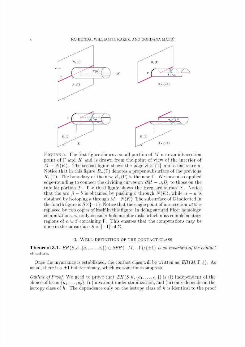
Figure 5. The first figure shows a small portion of M near an intersectionpoint of Γ and K and is drawn from the point of view of the interior of M − N (K ). The second figure shows the page S × {1} and a basis arc a.Notice that in this figure R+(Γ) denotes a proper subsurface of the previousR+(Γ). The boundary of the new R+(Γ) is the new Γ. We have also applied
edge-rounding to connect the dividing curves on ∂M − ∪iDi to those on thetubular portion T . The third figure shows the Heegaard surface Σ. Noticethat the arc β − b is obtained by pushing b through N (K ), while α − a isobtained by isotoping a through M − N (K ). The subsurface of Σ indicated inthe fourth figure is S ×{−1}. Notice that the single point of intersection a∩b isreplaced by two copies of itself in this figure. In doing sutured Floer homologycomputations, we only consider holomorphic disks which miss complementaryregions of α ∪ β containing Γ. This ensures that the computations may bedone in the subsurface S × {−1} of Σ.
3. Well-definition of the contact class
Theorem 3.1. EH (S,h, {a1, . . . , ar}) ∈ SFH (−M, −Γ)/{±1} is an invariant of the contact structure.
Once the invariance is established, the contact class will be written as EH (M, Γ, ξ). Asusual, there is a ±1 indeterminacy, which we sometimes suppress.
Outline of Proof. We need to prove that EH (S,h, {a1, . . . , ar}) is (i) independent of thechoice of basis {a1, . . . , ar}, (ii) invariant under stabilization, and (iii) only depends on theisotopy class of h. The dependence only on the isotopy class of h is identical to the proof
8/3/2019 Ko Honda, William H. Kazez and Gordana Matic- The Contact Invariant in Sutured Floer Homology
http://slidepdf.com/reader/full/ko-honda-william-h-kazez-and-gordana-matic-the-contact-invariant-in-sutured 9/34
THE CONTACT INVARIANT IN SUTURED FLOER HOMOLOGY 9
Γ
x
α
β
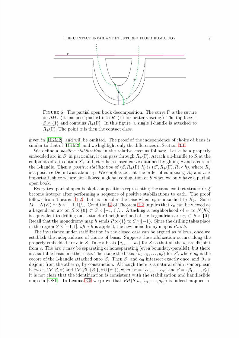
Figure 6. The partial open book decomposition. The curve Γ is the suture
on ∂M . (It has been pushed into R+(Γ) for better viewing.) The top face isS × {1} and contains R+(Γ). In this figure, a single 1-handle is attached to
R+(Γ). The point x is then the contact class.
given in [HKM2], and will be omitted. The proof of the independence of choice of basis issimilar to that of [HKM2], and we highlight only the differences in Section 3.1.
We define a positive stabilization in the relative case as follows: Let c be a properlyembedded arc in S ; in particular, it can pass through R+(Γ). Attach a 1-handle to S at theendpoints of c to obtain S ′, and let γ be a closed curve obtained by gluing c and a core of the 1-handle. Then a positive stabilization of (S, R+(Γ), h) is (S ′, R+(Γ), Rγ ◦ h), where Rγ
is a positive Dehn twist about γ . We emphasize that the order of composing Rγ and h is
important, since we are not allowed a global conjugation of S when we only have a partialopen book.
Every two partial open book decompositions representing the same contact structure ξbecome isotopic after performing a sequence of positive stabilizations to each. The proof follows from Theorem 1.2: Let us consider the case when c0 is attached to K 0. SinceM − N (K ) ≃ S × [−1, 1]/∼, Condition 4 of Theorem 1.2 implies that c0 can be viewed asa Legendrian arc on S × {0} ⊂ S × [−1, 1]/∼. Attaching a neighborhood of c0 to N (K 0)is equivalent to drilling out a standard neighborhood of the Legendrian arc c0 ⊂ S × {0}.Recall that the monodromy map h sends P × {1} to S × {−1}. Since the drilling takes placein the region S × [−1, 1], after h is applied, the new monodromy map is Rγ ◦ h.
The invariance under stabilization in the closed case can be argued as follows, once we
establish the independence of choice of basis: Suppose the stabilization occurs along theproperly embedded arc c in S . Take a basis {a1, . . . , ar} for S so that all the ai are disjointfrom c. The arc c may be separating or nonseparating (even boundary-parallel), but thereis a suitable basis in either case. Then take the basis {a0, a1, . . . , ar} for S ′, where a0 is thecocore of the 1-handle attached onto S . Then β 0 and α0 intersect exactly once, and β 0 isdisjoint from the other αi by construction. Although there is a natural chain isomorphismbetween CF (β, α) and CF (β ∪{β 0}, α∪{α0}), where α = {α1, . . . , αr} and β = {β 1, . . . , β r},it is not clear that the identification is consistent with the stabilization and handleslidemaps in [OS1]. In Lemma 3.5 we prove that EH (S,h, {a1, . . . , ar}) is indeed mapped to
8/3/2019 Ko Honda, William H. Kazez and Gordana Matic- The Contact Invariant in Sutured Floer Homology
http://slidepdf.com/reader/full/ko-honda-william-h-kazez-and-gordana-matic-the-contact-invariant-in-sutured 10/34
10 KO HONDA, WILLIAM H. KAZEZ, AND GORDANA MATIC
EH (S ′, h′, {a0, . . . , ar}) under the stabilization and handleslide maps in [OS1]. (Notice thatthis proof of invariance could have been used in [HKM2] without appealing to the equivalence
with the Ozsvath-Szabo contact invariant. This was pointed out to the authors by AndrasStipsicz.)Now, if R+(Γ) is not a homotopically trivial disk, then it is not always possible to find
a basis {a1, . . . , ar} which is disjoint from the arc of stabilization c. This difficulty is dealtwith in Section 3.2.
3.1. Change of basis. Let {a1, a2, . . . , ar} be a basis for (S, R+(Γ)). After possibly re-ordering the ai’s, suppose a1 and a2 are adjacent arcs on A = ∂P − Γ, i.e., there is an arcτ ⊂ A with endpoints on a1 and a2 such that τ does not intersect any ai in int(τ ). Definea1 + a2 as the isotopy class of a1 ∪ τ ∪ a2, relative to the endpoints. Then the modification{a1, a2, . . . , ar} → {a1 + a2, a2, . . . , ar} is called an arc slide.
Lemma 3.2. EH (S, h) is invariant under an arc slide {a1, a2, . . . , ar} → {a1+a2, a2, . . . , ar}.
Proof. Same as that of Lemma 3.4 of [HKM2].
Let {a1, . . . , ar} and {b1, . . . , br} be two bases for (S, R+(Γ)). Assume that the two basesintersect transversely and efficiently , i.e., each pair of arcs ai, b j realizes the minimum numberof intersections in its isotopy class, where the endpoints of the arcs are allowed to move inA. In particular, there are no bigons consisting of a subarc of ai and a subarc of b j , and notriangles consisting of a subarc of ai, a subarc of b j , and a subarc of A.
Lemma 3.3. Suppose that each component of P intersects Γ along at least two arcs. Then there is a sequence of arc slides which takes {a1, . . . , ar} to {b1, . . . , br}.
Here P is the closure of P . The condition of the lemma is easily satisfied by performing atrivial stabilization along a boundary-parallel arc. Moreover, a trivial stabilization is easilyseen to preserve the EH class.
Proof. Consider a connected component Q of S − ∪ri=1ai − R+(Γ). Then Q is a (partially
open) polygon whose boundary ∂Q consists of 2k arcs, k−1 of which are ai or a−1i , k of whichare subarcs τ 1, . . . , τ k of ∂P − Γ, and one which is a subarc γ of Γ. (For the moment we haveoriented the ai, and the notation a−1i means that the orientation of ai and the orientation of ∂Q are opposite.) Since each component of P intersects Γ along at least two arcs, there isat least one arc c ⊂ ∂Q of type ai or a−1i so that c−1 does not appear on ∂Q. Otherwise, Qglues up to a component of P whose closure intersects Γ along one arc.
Suppose (ri=1 ai) ∩ (ri=1 bi) = 0. We will apply a sequence of arc slides to {ai}ri=1 toobtain {a′i}
ri=1 which is disjoint from {bi}
ri=1. After possibly reordering the arcs, there is a
subarc b01 ⊂ b1 in Q with endpoints on a1 and τ 1 on ∂Q. The subarc b01 separates Q into tworegions Q1 and Q2, only one of which (say Q1) has γ as a boundary arc. If c = a1, then wecan slide c around the boundary of Q2 to obtain a′1 which has fewer intersections with b1. If a1 and a−11 both occur on ∂Q, then we have a problem if Q1 has γ as a boundary arc and Q2
has a−11 as a boundary arc. To maneuver around this problem, move c via a sequence of arcslides so that the resulting c′ is parallel to γ (and protects it). Then we can slide a1 aroundthe boundary of ∂Q1 as in [HKM2].
8/3/2019 Ko Honda, William H. Kazez and Gordana Matic- The Contact Invariant in Sutured Floer Homology
http://slidepdf.com/reader/full/ko-honda-william-h-kazez-and-gordana-matic-the-contact-invariant-in-sutured 11/34
THE CONTACT INVARIANT IN SUTURED FLOER HOMOLOGY 11
Finally, suppose that {ai}ri=1 and {bi}r
i=1 are disjoint. Let Q be a component of S − ∪iai −
R+(Γ), as before. Let b1 be an arc in Q which is not parallel to any ai or a−1i . The arc b1
cuts Q into two components Q1 and Q2, where Q1 has γ as a boundary arc. We claim thatthere is some ai on ∂Q2 so that a−1i is not on ∂Q2. Otherwise, the arcs on ∂Q2 will be pairedup and b1 will cut off a subsurface of S whose closure does not intersect Γ. Moreover, wemay also assume that ai is not parallel to any b j . Now, apply a sequence of arc slides to ai
so that it becomes parallel to b1.
3.2. Stabilization. A properly embedded arc c in S that intersects Γ efficiently is saidto have complexity n if there are n subarcs of c in P , both of whose endpoints are on Γ.Let (S ′, h′) be a positive stabilization of a partial open book decomposition (S, h) along aproperly embedded arc c ⊂ S that intersects Γ efficiently. Then (S ′, h′) is a stabilization of (S, h) of complexity n if c has complexity n.
The following lemma gives the fundamental property of arcs of complexity zero:
Lemma 3.4. An arc c has complexity zero if and only if there is a basis for (S, R+(Γ)) which is disjoint from c.
Proof. If an arc c has complexity > 0, then there is a subarc c0 ⊂ c in P , both of whoseendpoints are on Γ. It is impossible to find a basis that does not intersect c0, since the pair(c0, ∂c0) is homotopically nontrivial in (P , Γ).
On the other hand, suppose the complexity is zero. Then there are at most two subarcsof c ∩ P . If c lies in R+(Γ), then it does not intersect any basis of (S, R+(Γ)). If c is entirelycontained in P , then it is easy to see that there is a basis which avoids c. (There are twocases, depending on whether c cuts off a subsurface of P whose boundary does not intersectΓ.) Let ci be a subarc of c ∩ P . Depending on c, there may be two such, i.e., i = 1, 2, oronly one such, i.e., i = 1. In either case, for each ci, one of its endpoints is on Γ and theother on ∂P − Γ. If ci is a trivial subarc, i.e., forms a triangle in P , together with an arcof Γ and an arc of ∂P − Γ, then ci does not obstruct the formation of a basis and can infact be isotoped out of P . Therefore assume that ci is nontrivial. Let τ 1, γ , τ 2 be subarcs of ∂P in counterclockwise order, where γ ⊂ Γ contains an endpoint of c1, and τ i are subarcsof ∂P − Γ. Also let τ be the component of ∂P − Γ with the other endpoint of c1. Thentake the first arc a of the basis to be parallel to c1, with endpoints on either τ and τ 1 or τ and τ 2. We have a choice of either of these unless c2 also has an endpoint on γ , in whichcase only one of these will work (and not intersect c2). The nontriviality of c1 implies thata is neither boundary-parallel, i.e., cuts off a disk in P , nor parallel to Γ. If the arc a cutsoff a subsurface of P whose boundary does not intersect Γ, then we must replace it withdisjoint, nonseparating arcs a1, . . . , a2g, where g is the genus of the cut-off surface. Oncewe cut P along a or a1, . . . , a2g, then c1 becomes trivial in the cut-open surface, and can beignored. We apply the same technique to c2, if necessary, and the rest of the basis can befound without difficulty.
Lemma 3.5. Let (S ′, h′) be a stabilization of (S, h) along an arc c of complexity zero. Suppose{a1, . . . , ar} is a basis for S which is disjoint from c and {a0, a1, . . . , ar} is a basis for S ′,where a0 is the cocore of the 1-handle attached to obtain S ′. Then EH (S,h, {a1, . . . , ar}) is
8/3/2019 Ko Honda, William H. Kazez and Gordana Matic- The Contact Invariant in Sutured Floer Homology
http://slidepdf.com/reader/full/ko-honda-william-h-kazez-and-gordana-matic-the-contact-invariant-in-sutured 12/34
12 KO HONDA, WILLIAM H. KAZEZ, AND GORDANA MATIC
mapped to EH (S ′, h′, {a0, . . . , ar}) under the stabilization and handleslide maps defined in [OS1].
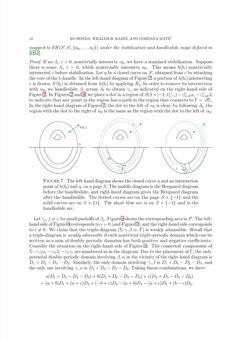
Proof. If no β i, i > 0, nontrivially intersects α0, we have a standard stabilization. Supposethere is some β i, i > 0, which nontrivially intersects α0. This means h(bi) nontriviallyintersected c before stabilization. Let η be a closed curve on S ′, obtained from c by attachingthe core of the 1-handle. In the left-hand diagram of Figure 7, a portion of h(bi) intersectingc is drawn; h′(bi) is obtained from h(bi) by applying Rη. In order to remove its intersectionwith α0, we handleslide β i across β 0 to obtain γ i, as indicated on the right-hand side of Figure 7. In Figures 7 and 8, we place a dot in a region of ∂ (S × [−1, 1]/∼) − ∪r
i=0αi − ∪ri=0β i
to indicate that any point in the region has a path in the region that connects to Γ = ∂ Σ.In the right-hand diagram of Figure 7, the dot to the left of α0 is clear; by following β 0, theregion with the dot to the right of α0 is the same as the region with the dot to the left of α0.
η
h(bi)
α0
β 0
x0
Figure 7. The left-hand diagram shows the closed curve η and an intersectionpoint of h(bi) and η, on a page S . The middle diagram is the Heegaard diagrambefore the handleslide, and right-hand diagram gives the Heegaard diagramafter the handleslide. The dotted curves are on the page S × {−1} and thesolid curves are on S × {1}. The short blue arc is on S × {−1} and is thehandleslide arc.
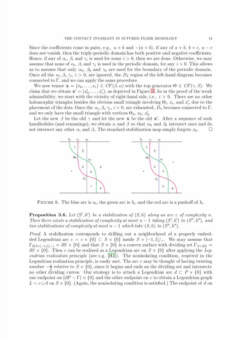
Let γ j, j = i, be small pushoffs of β j. Figure 8 shows the corresponding arcs in P . The left-hand side of Figure 8 corresponds to i = 0 (and Figure 7), and the right-hand side correspondsto i = 0. We claim that the triple-diagram (Σ,γ ,β ,α, Γ) is weakly admissible. Recall thata triple-diagram is weakly admissible if each nontrivial triply-periodic domain which can be
written as a sum of doubly-periodic domains has both positive and negative coefficients.Consider the situation on the right-hand side of Figure 8. The connected components of Σ − ∪iαi − ∪iβ i − ∪iγ i are numbered as in the diagram. Due to the placement of Γ, the onlypotential doubly-periodic domain involving β, α in the vicinity of the right-hand diagram isD1 + D2 − D4 − D5. Similarly, the only domain involving γ, β is D1 + D6 − D3 − D4, andthe only one involving γ, α is D2 + D3 − D5 − D6. Taking linear combinations, we have
a(D1 + D2 − D4 − D5) + b(D1 + D6 − D3 − D4) + c(D2 + D3 − D5 − D6)
= (a + b)D1 + (a + c)D2 + (−b + c)D3 − (a + b)D4 − (a + c)D5 + (b − c)D6.
8/3/2019 Ko Honda, William H. Kazez and Gordana Matic- The Contact Invariant in Sutured Floer Homology
http://slidepdf.com/reader/full/ko-honda-william-h-kazez-and-gordana-matic-the-contact-invariant-in-sutured 13/34
THE CONTACT INVARIANT IN SUTURED FLOER HOMOLOGY 13
Since the coefficients come in pairs, e.g., a + b and −(a + b), if any of a + b, b + c, a − cdoes not vanish, then the triply-periodic domain has both positive and negative coefficients.
Hence, if any of αi, β i and γ i is used for some i > 0, then we are done. Otherwise, we mayassume that none of αi, β i and γ i is used in the periodic domain, for any i > 0. This allowsus to assume that only α0, β 0 and γ 0 are used for the boundary of the periodic domain.Once all the αi, β i, γ i, i > 0, are ignored, the D4 region of the left-hand diagram becomesconnected to Γ, and we can apply the same procedure.
We now tensor x = (x0, . . . , xr) ∈ CF (β, α) with the top generator Θ ∈ CF (γ, β ). Weclaim that we obtain x′ = (x′0, . . . , x′r), as depicted in Figure 8. As in the proof of the weakadmissibility, we start with the vicinity of right-hand side, i.e., i > 0. There are no otherholomorphic triangles besides the obvious small triangle involving Θi, xi, and x′i, due to theplacement of the dots. Once the αi, β i, γ i, i > 0, are exhausted, D4 becomes connected to Γ,and we only have the small triangle with vertices Θ0, x0, x′0.
Let the new β be the old γ and let the new x be the old x′
. After a sequence of suchhandleslides (and renamings), we obtain α and β so that α0 and β 0 intersect once and donot intersect any other αi and β i. The standard stabilization map simply forgets x0.
Figure 8. The blue arc is ai, the green arc is bi, and the red arc is a pushoff of bi.
Proposition 3.6. Let (S ′, h′) be a stabilization of (S, h) along an arc c of complexity n.Then there exists a stabilization of complexity at most n − 1 taking (S ′, h′) to (S ′′, h′′), and two stabilizations of complexity at most n − 1 which take (S, h) to (S ′′, h′′).
Proof. A stabilization corresponds to drilling out a neighborhood of a properly embed-
ded Legendrian arc c = c × {0} ⊂ S × {0} inside S × [−1, 1]/∼. We may assume thatΓ∂ (S ×[−1,1]/∼) = ∂S × {0} and that S × {0} is a convex surface with dividing set ΓS ×{0} =∂S × {0}. Then c can be realized as a Legendrian arc on S × {0} after applying the Leg-endrian realization principle (see e.g. [H1]). The nonisolating condition, required in theLegendrian realization principle, is easily met. The arc c may be thought of having twistingnumber −1
2relative to S × {0}, since it begins and ends on the dividing set and intersects
no other dividing curves. Our strategy is to attach a Legendrian arc d ⊂ P × {0} withone endpoint on (∂P − Γ) × {0} and the other endpoint on c to obtain a Legendrian graphL = c ∪ d on S × {0}. (Again, the nonisolating condition is satisfied.) The endpoint of d on
8/3/2019 Ko Honda, William H. Kazez and Gordana Matic- The Contact Invariant in Sutured Floer Homology
http://slidepdf.com/reader/full/ko-honda-william-h-kazez-and-gordana-matic-the-contact-invariant-in-sutured 14/34
14 KO HONDA, WILLIAM H. KAZEZ, AND GORDANA MATIC
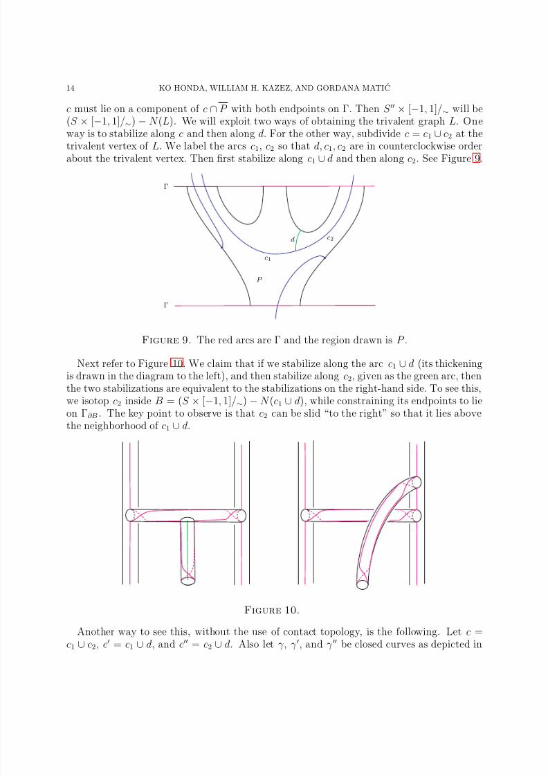
c must lie on a component of c ∩ P with both endpoints on Γ. Then S ′′ × [−1, 1]/∼ will be(S × [−1, 1]/∼) − N (L). We will exploit two ways of obtaining the trivalent graph L. One
way is to stabilize along c and then along d. For the other way, subdivide c = c1 ∪ c2 at thetrivalent vertex of L. We label the arcs c1, c2 so that d, c1, c2 are in counterclockwise orderabout the trivalent vertex. Then first stabilize along c1 ∪ d and then along c2. See Figure 9.
d
c1
c2
P
Γ
Γ
Figure 9. The red arcs are Γ and the region drawn is P .
Next refer to Figure 10. We claim that if we stabilize along the arc c1 ∪ d (its thickeningis drawn in the diagram to the left), and then stabilize along c2, given as the green arc, thenthe two stabilizations are equivalent to the stabilizations on the right-hand side. To see this,we isotop c2 inside B = (S × [−1, 1]/∼) − N (c1 ∪ d), while constraining its endpoints to lieon Γ∂B . The key point to observe is that c2 can be slid “to the right” so that it lies abovethe neighborhood of c1 ∪ d.
Figure 10.
Another way to see this, without the use of contact topology, is the following. Let c =c1 ∪ c2, c′ = c1 ∪ d, and c′′ = c2 ∪ d. Also let γ , γ ′, and γ ′′ be closed curves as depicted in
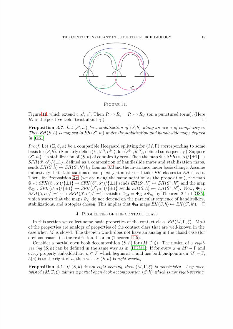
8/3/2019 Ko Honda, William H. Kazez and Gordana Matic- The Contact Invariant in Sutured Floer Homology
http://slidepdf.com/reader/full/ko-honda-william-h-kazez-and-gordana-matic-the-contact-invariant-in-sutured 15/34
THE CONTACT INVARIANT IN SUTURED FLOER HOMOLOGY 15
γ
γ ′ γ ′′
Figure 11.
Figure 11, which extend c, c′
, c′′
. Then Rγ ′ ◦ Rγ = Rγ ′′ ◦ Rγ ′ (on a punctured torus). (HereRγ is the positive Dehn twist about γ .)
Proposition 3.7. Let (S ′, h′) be a stabilization of (S, h) along an arc c of complexity n.Then EH (S, h) is mapped to EH (S ′, h′) under the stabilization and handleslide maps defined in [OS1].
Proof. Let (Σ, β , α) be a compatible Heegaard splitting for (M, Γ) corresponding to somebasis for (S, h). (Similarly define (Σ, β (i), α(i)), for (S (i), h(i)), defined subsequently.) Suppose(S ′, h′) is a stabilization of (S, h) of complexity zero. Then the map Φ : SFH (β, α)/{±1} →SFH (β ′, α′)/{±1}, defined as a composition of handleslide maps and stabilization maps,sends EH (S, h) → EH (S ′, h′) by Lemma 3.5 and the invariance under basis change. Assume
inductively that stabilizations of complexity at most n − 1 take EH classes to EH classes.Then, by Proposition 3.6 (we are using the same notation as the proposition), the mapΦ12 : SFH (β ′, α′)/{±1} → SFH (β ′′, α′′)/{±1} sends EH (S ′, h′) → EH (S ′′, h′′) and the mapΦ02 : SFH (β, α)/{±1} → SFH (β ′′, α′′)/{±1} sends EH (S, h) → EH (S ′′, h′′). Now, Φ01 :SFH (β, α)/{±1} → SFH (β ′, α′)/{±1} satisfies Φ02 = Φ12 ◦ Φ01 by Theorem 2.1 of [OS5],which states that the maps Φij do not depend on the particular sequence of handleslides,stabilizations, and isotopies chosen. This implies that Φ01 maps EH (S, h) → EH (S ′, h′).
4. Properties of the contact class
In this section we collect some basic properties of the contact class EH (M, Γ, ξ). Mostof the properties are analogs of properties of the contact class that are well-known in thecase when M is closed. The theorem which does not have an analog in the closed case (forobvious reasons) is the restriction theorem (Theorem 4.5).
Consider a partial open book decomposition (S, h) for (M, Γ, ξ). The notion of a right-veering (S, h) can be defined in the same way as in [HKM1]: If for every x ∈ ∂P − Γ andevery properly embedded arc a ⊂ P which begins at x and has both endpoints on ∂P − Γ,h(a) is to the right of a, then we say (S, h) is right-veering .
Proposition 4.1. If (S, h) is not right-veering, then (M, Γ, ξ) is overtwisted. Any over-twisted (M, Γ, ξ) admits a partial open book decomposition (S, h) which is not right-veering.
8/3/2019 Ko Honda, William H. Kazez and Gordana Matic- The Contact Invariant in Sutured Floer Homology
http://slidepdf.com/reader/full/ko-honda-william-h-kazez-and-gordana-matic-the-contact-invariant-in-sutured 16/34
16 KO HONDA, WILLIAM H. KAZEZ, AND GORDANA MATIC
Proof. The first assertion is proved in the same way as the analogous statement in [HKM1].For the second assertion, note that Example 1 of Section 5 gives a partial open book
decomposition of a neighborhood of an overtwisted disk with a left-veering arc. Attach theneighborhood of a Legendrian arc a which connects the boundary of the overtwisted disk toΓ ⊂ ∂M , and then complete it to a partial open book for (M, Γ). The left-veering arc fromExample 1 survives to give a left-veering arc.
Proposition 4.2. If (M, Γ, ξ) admits a partial open book decomposition (S, h) which is not right-veering, then EH (M, Γ, ξ) = 0.
Proof. Same as that of [HKM2].
By combining Propositions 4.1 and 4.2, we obtain the following:
Corollary 4.3. If (M, Γ, ξ) is overtwisted, then EH (M, Γ, ξ) = 0.
The next proposition describes the effect of Legendrian surgery on the contact invariant.
Proposition 4.4. If EH (M, Γ, ξ) = 0 and (M ′, Γ′, ξ′) is obtained from (M, Γ, ξ) by a Leg-endrian (−1)-surgery along a closed Legendrian curve L, then EH (M ′, Γ′, ξ′) = 0.
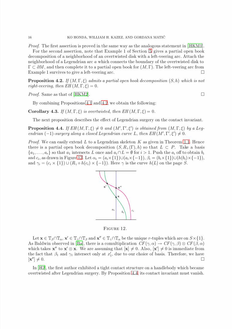
Proof. We can easily extend L to a Legendrian skeleton K as given in Theorem 1.1. Hencethere is a partial open book decomposition (S, R+(Γ), h) so that L ⊂ P . Take a basis{a1, . . . , ar} so that a1 intersects L once and ai ∩ L = ∅ for i > 1. Push the ai off to obtain biand ci, as drawn in Figure 12. Let αi = (ai×{1})∪(ai×{−1}), β i = (bi×{1})∪(h(bi)×{−1}),and γ i = (ci × {1}) ∪ (Rγ ◦ h(ci) × {−1}). Here γ is the curve h(L) on the page S .
aibi
ci
x
x′ x′′
Figure 12.
Let x ∈ Tβ ∩Tα, x′ ∈ Tγ ∩Tβ and x′′ ∈ Tγ ∩Tα be the unique r-tuples which are on S ×{1}.As Baldwin observed in [Ba], there is a comultiplication CF (γ, α) → CF (γ, β ) ⊗ CF (β, α)which takes x′′ to x′ ⊗ x. We are assuming that [x] = 0. Also, [x′] = 0 is immediate fromthe fact that β 1 and γ 1 intersect only at x′1, due to our choice of basis. Therefore, we have[x′′] = 0.
In [H2], the first author exhibited a tight contact structure on a handlebody which becameovertwisted after Legendrian surgery. By Proposition 4.4, its contact invariant must vanish.
8/3/2019 Ko Honda, William H. Kazez and Gordana Matic- The Contact Invariant in Sutured Floer Homology
http://slidepdf.com/reader/full/ko-honda-william-h-kazez-and-gordana-matic-the-contact-invariant-in-sutured 17/34
THE CONTACT INVARIANT IN SUTURED FLOER HOMOLOGY 17
Theorem 4.5. Let (M, ξ) be a closed contact 3-manifold and N ⊂ M be a compact sub-manifold (without any closed components) with convex boundary and dividing set Γ. If
EH (M, ξ) = 0, then EH (N, Γ, ξ|N ) = 0.Proof. Consider the partial open book decomposition (S, R+(Γ), h) for (N, Γ, ξ|N ), obtainedby decomposing N into N (K ) and N − N (K ). Now, the complement N ′ = M − N can besimilarly decomposed into N (K ′) and N ′ − N (K ′), where K ′ is a Legendrian graph in N ′
with univalent vertices on Γ. We may assume that the univalent vertices of K ′ and K do notintersect. Then an open book decomposition for (M, ξ) can be obtained from the Heegaarddecomposition (N − N (K )) ∪ N (K ′) and (N ′ − N (K ′)) ∪ N (K ). Indeed, both handlebodiesare easily seen to be product disk decomposable. The page T for (M, ξ) can be obtainedfrom (S, R+(Γ), h) by successively attaching 1-handles, subject to the condition that none of
the handles be attached along ∂P , where P = S − R+(Γ). The monodromy map g : T → T extends h : P → S .
Let {a1, . . . , ar, a′1, . . . , a′s} be a basis for T which extends a basis {a1, . . . , ar} for (S, R+(Γ)).For such an extension to exist, T − P must be connected. This is possible if M − N is con-nected — simply take suitable stabilizations to connect up the components of T − P . If M − N is disconnected, we apply a standard contact connected sum inside M − N to con-nect up disjoint components of M − N . This has the effect of attaching 1-handles to T awayfrom P and extending the monodromy map by the identity. The contact manifold ( M, ξ) hasbeen modified, but it is easy to see that the contact class of the connected sum is nonzero if and only if the original contact class is nonzero.
Let x be the generator of EH (N, Γ, ξ|N ) with respect to {a1, . . . , ar} and (x, x′) be thegenerator of EH (M, ξ) with respect to {a1, . . . , ar, a′1, . . . , a′s}. If ∂ (
i ciyi) = x, then we
claim that ∂ (i ci(y
i,x′
)) = (x
,x′
). Indeed, each of the intersection points of x′
must mapto itself via the constant map — this uses up all the intersection points of x′. We thenerase all the αi and β i corresponding to x′, and are left with the Heegaard diagram for(S, R+(Γ)).
Comparison with other invariants. We now make some remarks on the relationship tothe contact invariant in the closed case and to Legendrian knot invariants.
1. If we start with a closed (M, ξ), then we can remove a standard contact 3-ball B3
with Γ∂B3 = S 1. The sutured manifold is called M (1) in Juhasz [Ju1]. In this case,
SFH (−M (1)) = HF (−M ), and the contact element in SFH (−M (1)) coincides with the
Ozsvath-Szabo contact class in HF (−M ). (Think of the disk R+ being squashed to a pointto give the basepoint z.)
2. A Legendrian knot L has a standard neighborhood N (L) which has convex boundary. Thedividing set Γ∂N (L) satisfies #Γ∂N (L) = 2 and |Γ∂N (L) ∩ ∂D2| = 2, where D2 is the meridianof N (L). Moreover, the framing for L induced by ξ agrees with the framing induced by theribbon in N (L) which contains L and has boundary on Γ∂N (L).
If (M, ξ) is closed, then EH (M − N (L), Γ∂N (L), ξ) is an invariant of the Legendrian knotL which sits in SFH (−(M − N (L)), −Γ∂N (L)). On the other hand, if we choose the sutureΓ on ∂N (L) to consist of two parallel meridian curves, then SFH (−(M − N (L)), −Γ) =
8/3/2019 Ko Honda, William H. Kazez and Gordana Matic- The Contact Invariant in Sutured Floer Homology
http://slidepdf.com/reader/full/ko-honda-william-h-kazez-and-gordana-matic-the-contact-invariant-in-sutured 18/34
18 KO HONDA, WILLIAM H. KAZEZ, AND GORDANA MATIC
HFK (−M, L). Hence we are slightly off from the Legendrian knot invariants of Ozsvath-Szabo-Thurston [OST] and Lisca-Ozsvath-Stipsicz-Szabo [LOSS] — the Legendrian knot
invariant currently does not sit in HFK (−M, L). We also only have one invariant, ratherthan two.
5. Examples
In this section we calculate a few basic examples.
Example 1: Standard neighborhood of an overtwisted disk. Let D be a convex surface whichis a slight outward extension of an overtwisted disk. Then consider its [0, 1]-invariant contactneighborhood M = D × [0, 1]. After rounding the edges, we obtain Γ∂M which consists of three closed curves, two which are γ × {0, 1}, where γ is a closed curve in the interior of D2,and one which is ∂D2 × {1
2}. Our Legendrian graph K is an arc { p} × [0, 1], where p ∈ γ .
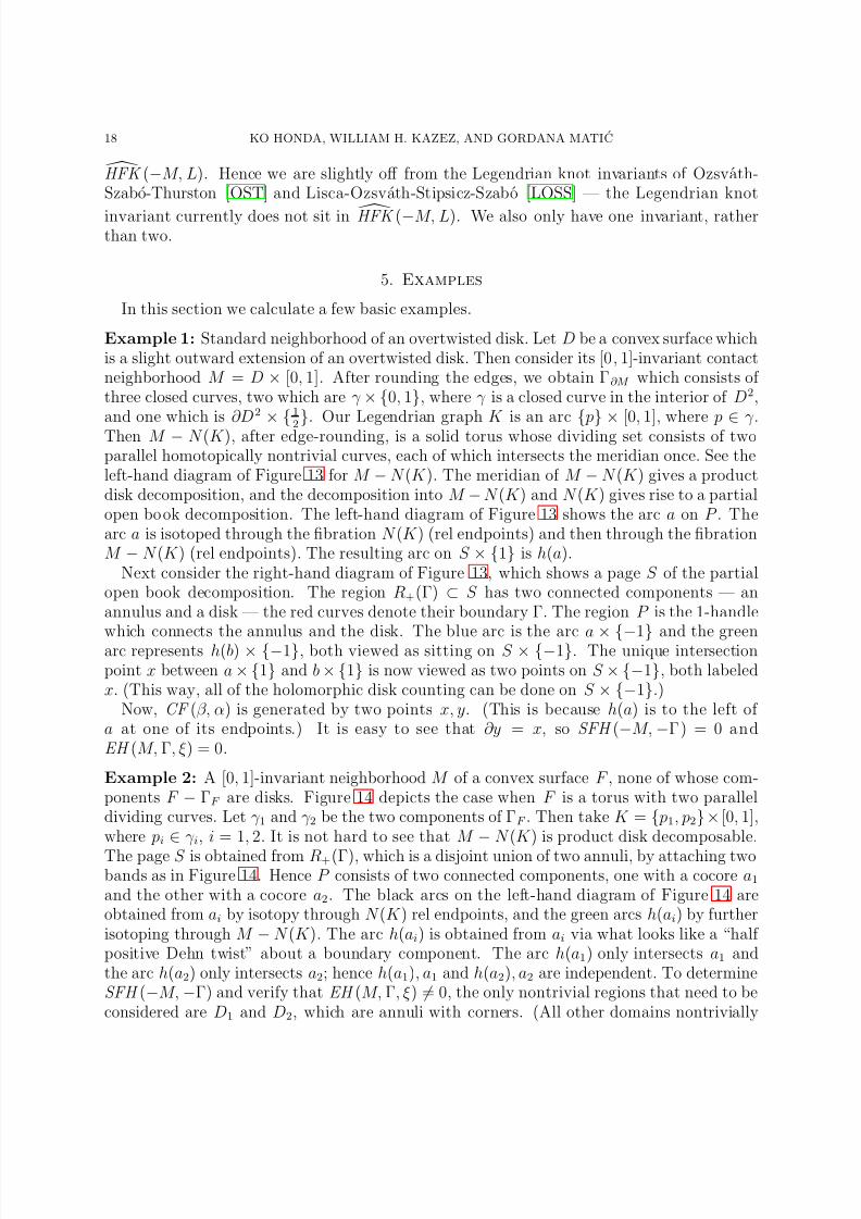
Then M − N (K ), after edge-rounding, is a solid torus whose dividing set consists of twoparallel homotopically nontrivial curves, each of which intersects the meridian once. See theleft-hand diagram of Figure 13 for M − N (K ). The meridian of M − N (K ) gives a productdisk decomposition, and the decomposition into M − N (K ) and N (K ) gives rise to a partialopen book decomposition. The left-hand diagram of Figure 13 shows the arc a on P . Thearc a is isotoped through the fibration N (K ) (rel endpoints) and then through the fibrationM − N (K ) (rel endpoints). The resulting arc on S × {1} is h(a).
Next consider the right-hand diagram of Figure 13, which shows a page S of the partialopen book decomposition. The region R+(Γ) ⊂ S has two connected components — anannulus and a disk — the red curves denote their boundary Γ. The region P is the 1-handlewhich connects the annulus and the disk. The blue arc is the arc a × {−1} and the greenarc represents h(b) × {−1}, both viewed as sitting on S × {−1}. The unique intersectionpoint x between a × {1} and b × {1} is now viewed as two points on S × {−1}, both labeledx. (This way, all of the holomorphic disk counting can be done on S × {−1}.)
Now, CF (β, α) is generated by two points x, y. (This is because h(a) is to the left of a at one of its endpoints.) It is easy to see that ∂y = x, so SFH (−M, −Γ) = 0 andEH (M, Γ, ξ) = 0.
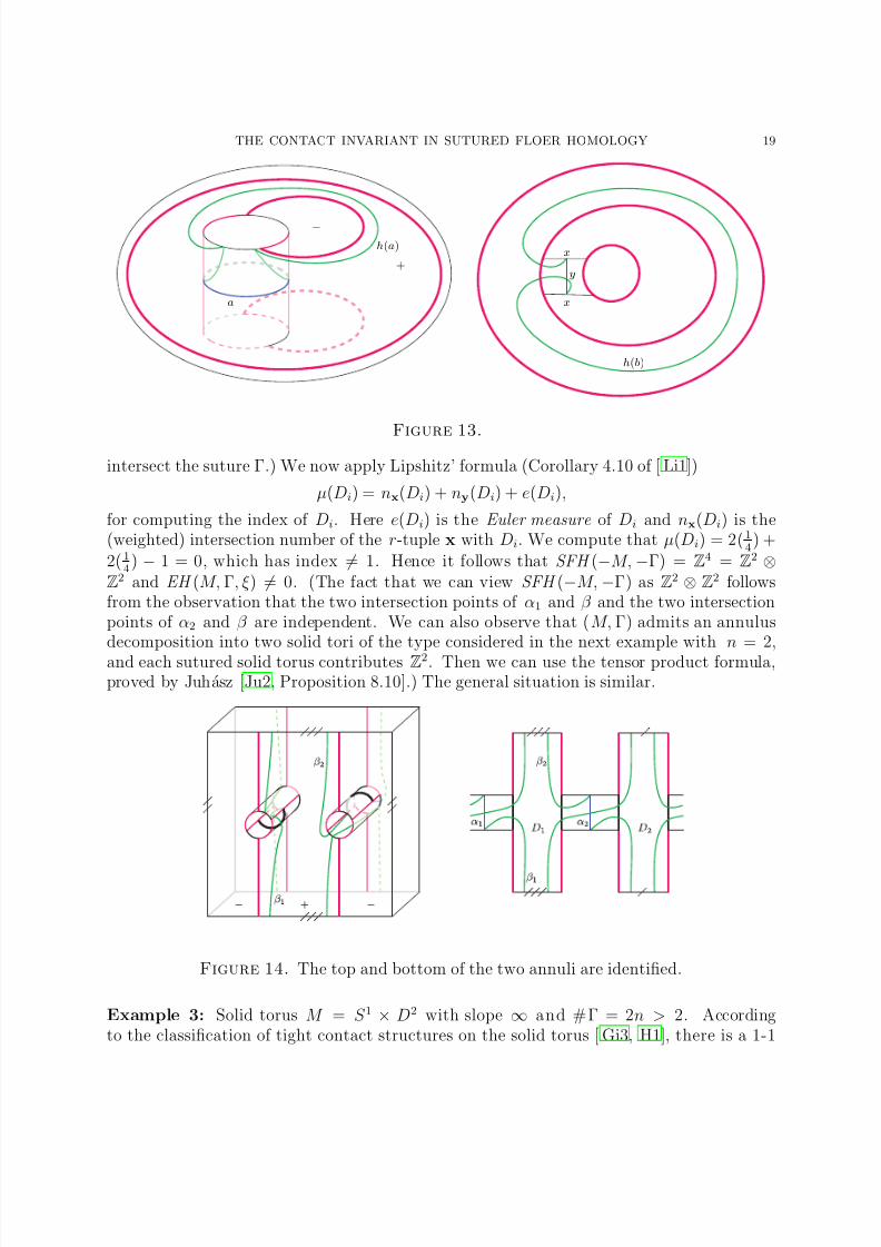
Example 2: A [0, 1]-invariant neighborhood M of a convex surface F , none of whose com-ponents F − ΓF are disks. Figure 14 depicts the case when F is a torus with two paralleldividing curves. Let γ 1 and γ 2 be the two components of ΓF . Then take K = { p1, p2}× [0, 1],where pi ∈ γ i, i = 1, 2. It is not hard to see that M − N (K ) is product disk decomposable.
The page S is obtained from R+(Γ), which is a disjoint union of two annuli, by attaching twobands as in Figure 14. Hence P consists of two connected components, one with a cocore a1
and the other with a cocore a2. The black arcs on the left-hand diagram of Figure 14 areobtained from ai by isotopy through N (K ) rel endpoints, and the green arcs h(ai) by furtherisotoping through M − N (K ). The arc h(ai) is obtained from ai via what looks like a “half positive Dehn twist” about a boundary component. The arc h(a1) only intersects a1 andthe arc h(a2) only intersects a2; hence h(a1), a1 and h(a2), a2 are independent. To determineSFH (−M, −Γ) and verify that EH (M, Γ, ξ) = 0, the only nontrivial regions that need to beconsidered are D1 and D2, which are annuli with corners. (All other domains nontrivially
8/3/2019 Ko Honda, William H. Kazez and Gordana Matic- The Contact Invariant in Sutured Floer Homology
http://slidepdf.com/reader/full/ko-honda-william-h-kazez-and-gordana-matic-the-contact-invariant-in-sutured 19/34
THE CONTACT INVARIANT IN SUTURED FLOER HOMOLOGY 19
a
h(a)
+
−
x
x
y
h(b)
Figure 13.
intersect the suture Γ.) We now apply Lipshitz’ formula (Corollary 4.10 of [ Li1])
µ(Di) = nx(Di) + ny(Di) + e(Di),
for computing the index of Di. Here e(Di) is the Euler measure of Di and nx(Di) is the(weighted) intersection number of the r-tuple x with Di. We compute that µ(Di) = 2(1
4) +
2(14
) − 1 = 0, which has index = 1. Hence it follows that SFH (−M, −Γ) = Z4 = Z2 ⊗Z2 and EH (M, Γ, ξ) = 0. (The fact that we can view SFH (−M, −Γ) as Z2 ⊗ Z2 followsfrom the observation that the two intersection points of α1 and β and the two intersectionpoints of α2 and β are independent. We can also observe that (M, Γ) admits an annulusdecomposition into two solid tori of the type considered in the next example with n = 2,and each sutured solid torus contributes Z2. Then we can use the tensor product formula,proved by Juhasz [Ju2, Proposition 8.10].) The general situation is similar.
Figure 14. The top and bottom of the two annuli are identified.
Example 3: Solid torus M = S 1 × D2 with slope ∞ and #Γ = 2n > 2. Accordingto the classification of tight contact structures on the solid torus [ Gi3, H1], there is a 1-1
8/3/2019 Ko Honda, William H. Kazez and Gordana Matic- The Contact Invariant in Sutured Floer Homology
http://slidepdf.com/reader/full/ko-honda-william-h-kazez-and-gordana-matic-the-contact-invariant-in-sutured 20/34
20 KO HONDA, WILLIAM H. KAZEZ, AND GORDANA MATIC
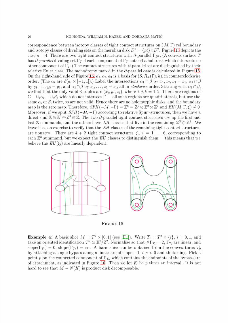
correspondence between isotopy classes of tight contact structures on (M, Γ) rel boundaryand isotopy classes of dividing sets on the meridian disk D2 = { pt}×D2. Figure 15 depicts the
case n = 4. There are two tight contact structures with ∂ -parallel ΓD2. (A convex surface T has ∂ -parallel dividing set ΓT if each component of ΓT cuts off a half-disk which intersects noother component of ΓT .) The contact structures with ∂ -parallel set are distinguished by theirrelative Euler class. The monodromy map h in the ∂ -parallel case is calculated in Figure 15.On the right-hand side of Figure 15, a1, a2, a3 is a basis for (S, R+(Γ), h), in counterclockwiseorder. (The αi are ∂ (ai × [−1, 1]).) Label the intersections α1 ∩ β by x1, x2, x3 = x1, α2 ∩ β by y1, . . . , y5 = y1, and α3 ∩ β by z1, . . . , z5 = z1, all in clockwise order. Starting with α1 ∩ β ,we find that the only valid 3-tuples are (xi, y j, zk), where i,j,k = 1, 2. There are regions of Σ − ∪iαi − ∪iβ j which do not intersect Γ — all such regions are quadrilaterals, but use thesame αi or β i twice, so are not valid. Hence there are no holomorphic disks, and the boundarymap is the zero map. Therefore, SFH (−M, −Γ) = Z8 = Z2 ⊗Z2 ⊗Z2 and EH (M, Γ, ξ) = 0.
Moreover, if we split SFH (−M, −Γ) according to relative Spinc
-structures, then we have adirect sum Z⊕Z3 ⊕Z3 ⊕Z. The two ∂ -parallel tight contact structures use up the first andlast Z summands, and the others have EH classes that live in the remaining Z3 ⊕ Z3. Weleave it as an exercise to verify that the EH classes of the remaining tight contact structuresare nonzero. There are 4 + 2 tight contact structures ξi, i = 1, . . . , 6, corresponding toeach Z3 summand, but we expect the EH classes to distinguish them — this means that webelieve the EH (ξi) are linearly dependent.
Figure 15.
Example 4: A basic slice M = T 2 × [0, 1] (see [H1]). Write T i = T 2 × {i}, i = 0, 1, andtake an oriented identification T 2 ≃ R2/Z2. Normalize so that #ΓT i = 2, ΓT i are linear, andslope(ΓT 1) = 0, slope(ΓT 0) = ∞. A basic slice can be obtained from the convex torus T 0by attaching a single bypass along a linear arc of slope −1 < s < 0 and thickening. Pick apoint p on the connected component of ΓT 0 which contains the endpoints of the bypass arcof attachment, as indicated in Figure 16. Then we let K be p times an interval. It is nothard to see that M − N (K ) is product disk decomposable.
8/3/2019 Ko Honda, William H. Kazez and Gordana Matic- The Contact Invariant in Sutured Floer Homology
http://slidepdf.com/reader/full/ko-honda-william-h-kazez-and-gordana-matic-the-contact-invariant-in-sutured 21/34
THE CONTACT INVARIANT IN SUTURED FLOER HOMOLOGY 21
p
−+ −+
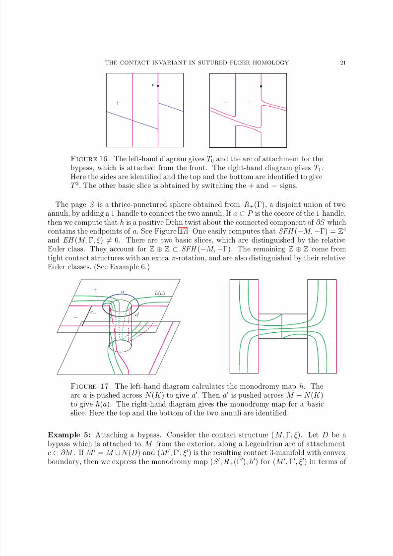
Figure 16. The left-hand diagram gives T 0 and the arc of attachment for thebypass, which is attached from the front. The right-hand diagram gives T 1.Here the sides are identified and the top and the bottom are identified to giveT 2. The other basic slice is obtained by switching the + and − signs.
The page S is a thrice-punctured sphere obtained from R+(Γ), a disjoint union of twoannuli, by adding a 1-handle to connect the two annuli. If a ⊂ P is the cocore of the 1-handle,then we compute that h is a positive Dehn twist about the connected component of ∂S whichcontains the endpoints of a. See Figure 17. One easily computes that SFH (−M, −Γ) = Z4
and EH (M, Γ, ξ) = 0. There are two basic slices, which are distinguished by the relativeEuler class. They account for Z ⊕ Z ⊂ SFH (−M, −Γ). The remaining Z ⊕ Z come fromtight contact structures with an extra π-rotation, and are also distinguished by their relativeEuler classes. (See Example 6.)
+
−
a h(a)
a′c−
Figure 17. The left-hand diagram calculates the monodromy map h. Thearc a is pushed across N (K ) to give a′. Then a′ is pushed across M − N (K )to give h(a). The right-hand diagram gives the monodromy map for a basicslice. Here the top and the bottom of the two annuli are identified.
Example 5: Attaching a bypass. Consider the contact structure (M, Γ, ξ). Let D be abypass which is attached to M from the exterior, along a Legendrian arc of attachmentc ⊂ ∂M . If M ′ = M ∪ N (D) and (M ′, Γ′, ξ′) is the resulting contact 3-manifold with convexboundary, then we express the monodromy map (S ′, R+(Γ′), h′) for (M ′, Γ′, ξ′) in terms of
8/3/2019 Ko Honda, William H. Kazez and Gordana Matic- The Contact Invariant in Sutured Floer Homology
http://slidepdf.com/reader/full/ko-honda-william-h-kazez-and-gordana-matic-the-contact-invariant-in-sutured 22/34
22 KO HONDA, WILLIAM H. KAZEZ, AND GORDANA MATIC
(S, R+(Γ), h) for (M, Γ, ξ). Assume without loss of generality that c does not intersect theneighborhood N (K ) of the Legendrian skeleton K for M . Let p1, p2 be the endpoints of c
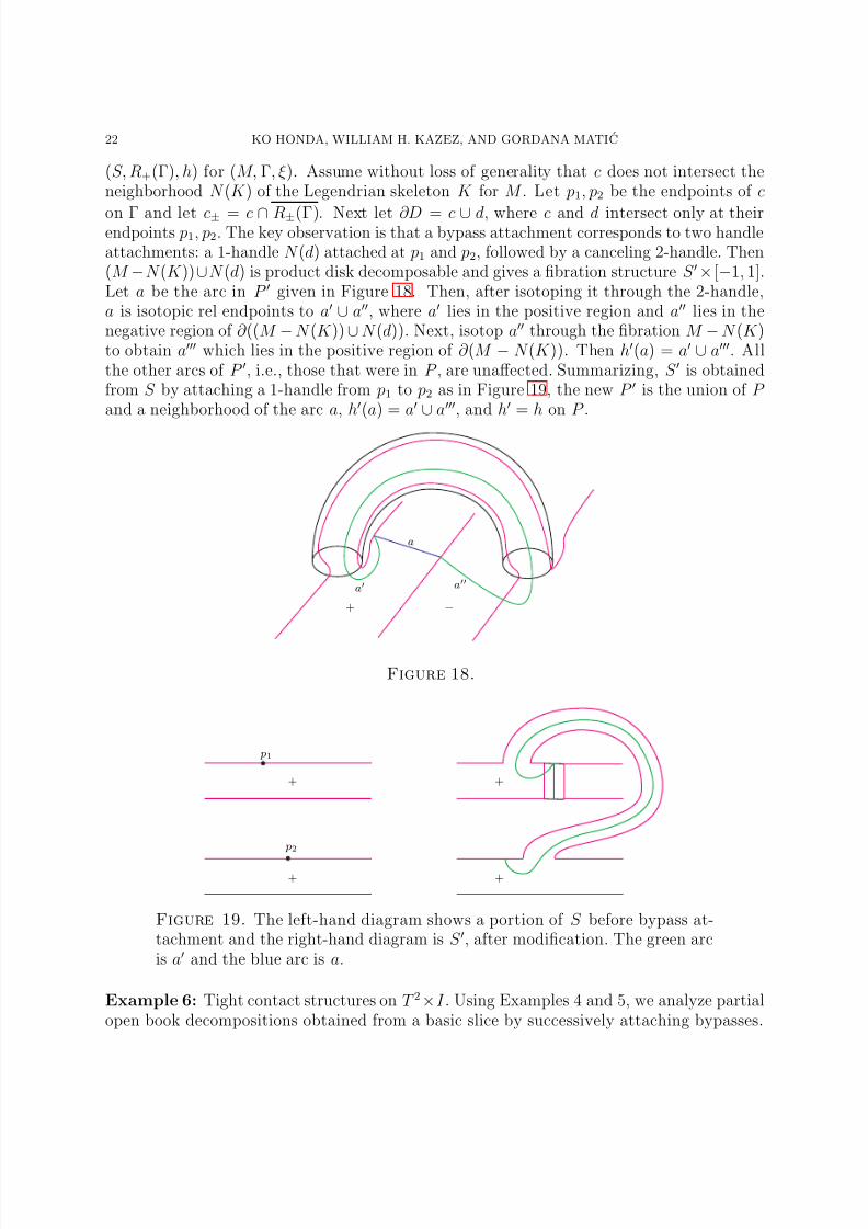
on Γ and let c± = c ∩ R±(Γ). Next let ∂D = c ∪ d, where c and d intersect only at theirendpoints p1, p2. The key observation is that a bypass attachment corresponds to two handleattachments: a 1-handle N (d) attached at p1 and p2, followed by a canceling 2-handle. Then(M −N (K ))∪N (d) is product disk decomposable and gives a fibration structure S ′×[−1, 1].Let a be the arc in P ′ given in Figure 18. Then, after isotoping it through the 2-handle,a is isotopic rel endpoints to a′ ∪ a′′, where a′ lies in the positive region and a′′ lies in thenegative region of ∂ ((M − N (K )) ∪ N (d)). Next, isotop a′′ through the fibration M − N (K )to obtain a′′′ which lies in the positive region of ∂ (M − N (K )). Then h′(a) = a′ ∪ a′′′. Allthe other arcs of P ′, i.e., those that were in P , are unaffected. Summarizing, S ′ is obtainedfrom S by attaching a 1-handle from p1 to p2 as in Figure 19, the new P ′ is the union of P and a neighborhood of the arc a, h′(a) = a′ ∪ a′′′, and h′ = h on P .
a
a′ a′′
+ −
Figure 18.
+
+
+
+
p1
p2
Figure 19. The left-hand diagram shows a portion of S before bypass at-tachment and the right-hand diagram is S ′, after modification. The green arcis a′ and the blue arc is a.
Example 6: Tight contact structures on T 2×I . Using Examples 4 and 5, we analyze partialopen book decompositions obtained from a basic slice by successively attaching bypasses.
8/3/2019 Ko Honda, William H. Kazez and Gordana Matic- The Contact Invariant in Sutured Floer Homology
http://slidepdf.com/reader/full/ko-honda-william-h-kazez-and-gordana-matic-the-contact-invariant-in-sutured 23/34
THE CONTACT INVARIANT IN SUTURED FLOER HOMOLOGY 23
These calculations were motivated by computations of open books for tight contact structureson T 3 by Van Horn-Morris [VH], and echo the results obtained there. In particular, we
will build up to an open book for the following tight contact structure on T 2
× [0, 4]: If (x,y,t) are coordinates on T 2 × [0, 4], then consider ker α, where α = cos(π2
t)dx − sin(π2
t)dy.Perturb ker α along ∂ (T 2 × [0, 4]) so that so it becomes convex with #ΓT 0 = #ΓT 4 = 2, andslope(ΓT 0) = slope(ΓT 4) = ∞.
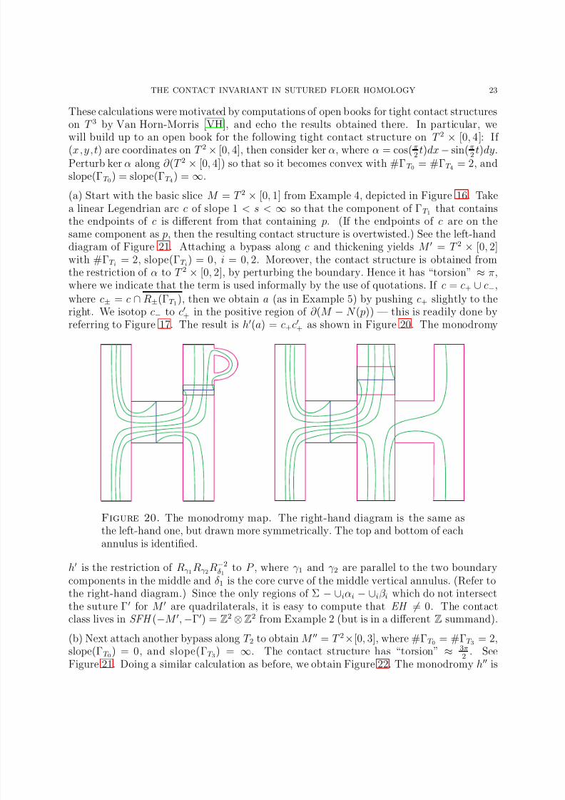
(a) Start with the basic slice M = T 2 × [0, 1] from Example 4, depicted in Figure 16. Takea linear Legendrian arc c of slope 1 < s < ∞ so that the component of ΓT 1 that containsthe endpoints of c is different from that containing p. (If the endpoints of c are on thesame component as p, then the resulting contact structure is overtwisted.) See the left-handdiagram of Figure 21. Attaching a bypass along c and thickening yields M ′ = T 2 × [0, 2]with #ΓT i = 2, slope(ΓT i) = 0, i = 0, 2. Moreover, the contact structure is obtained fromthe restriction of α to T 2 × [0, 2], by perturbing the boundary. Hence it has “torsion” ≈ π,where we indicate that the term is used informally by the use of quotations. If c = c+ ∪ c−,where c± = c ∩ R±(ΓT 1), then we obtain a (as in Example 5) by pushing c+ slightly to theright. We isotop c− to c′+ in the positive region of ∂ (M − N ( p)) — this is readily done byreferring to Figure 17. The result is h′(a) = c+c′+ as shown in Figure 20. The monodromy
Figure 20. The monodromy map. The right-hand diagram is the same asthe left-hand one, but drawn more symmetrically. The top and bottom of eachannulus is identified.
h′ is the restriction of Rγ 1Rγ 2R−2δ1
to P , where γ 1 and γ 2 are parallel to the two boundarycomponents in the middle and δ1 is the core curve of the middle vertical annulus. (Refer tothe right-hand diagram.) Since the only regions of Σ − ∪iαi − ∪iβ i which do not intersectthe suture Γ′ for M ′ are quadrilaterals, it is easy to compute that EH = 0. The contactclass lives in SFH (−M ′, −Γ′) = Z2 ⊗Z2 from Example 2 (but is in a different Z summand).
(b) Next attach another bypass along T 2 to obtain M ′′ = T 2×[0, 3], where #ΓT 0 = #ΓT 3 = 2,slope(ΓT 0) = 0, and slope(ΓT 3) = ∞. The contact structure has “torsion” ≈ 3π
2. See
Figure 21. Doing a similar calculation as before, we obtain Figure 22. The monodromy h′′ is
8/3/2019 Ko Honda, William H. Kazez and Gordana Matic- The Contact Invariant in Sutured Floer Homology
http://slidepdf.com/reader/full/ko-honda-william-h-kazez-and-gordana-matic-the-contact-invariant-in-sutured 24/34
24 KO HONDA, WILLIAM H. KAZEZ, AND GORDANA MATIC
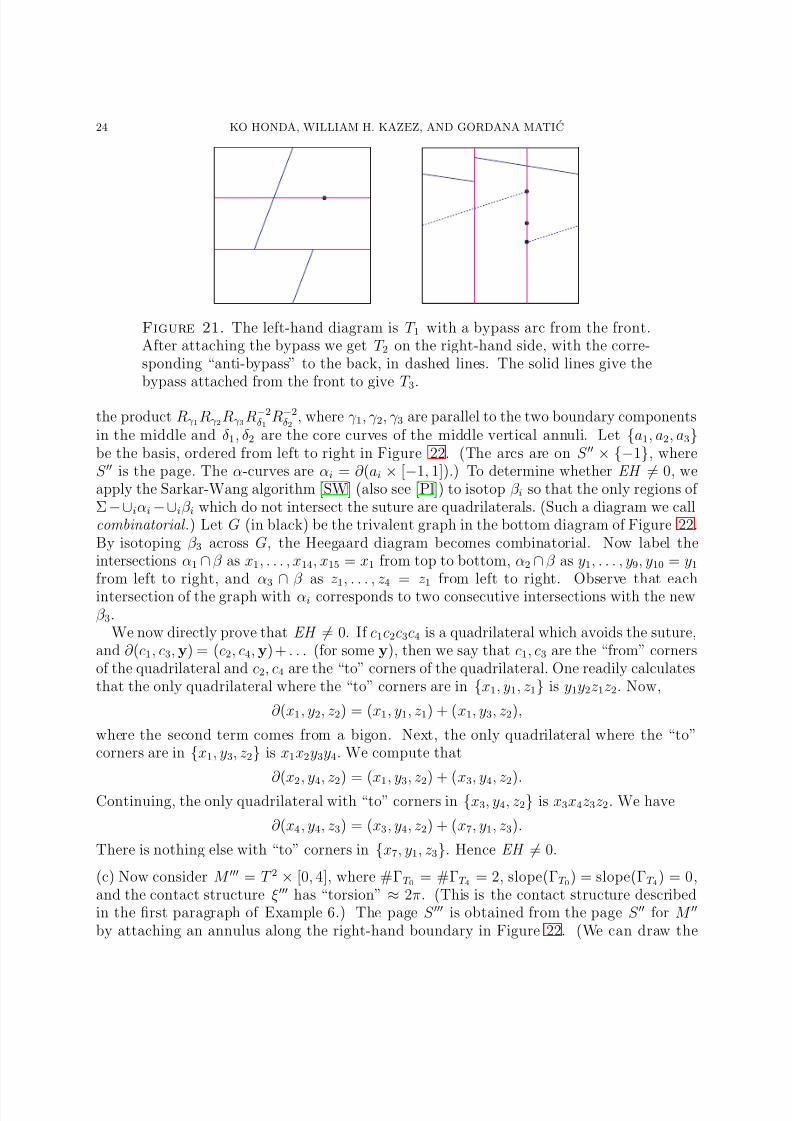
Figure 21. The left-hand diagram is T 1 with a bypass arc from the front.After attaching the bypass we get T 2 on the right-hand side, with the corre-sponding “anti-bypass” to the back, in dashed lines. The solid lines give thebypass attached from the front to give T 3.
the product Rγ 1Rγ 2Rγ 3R−2δ1
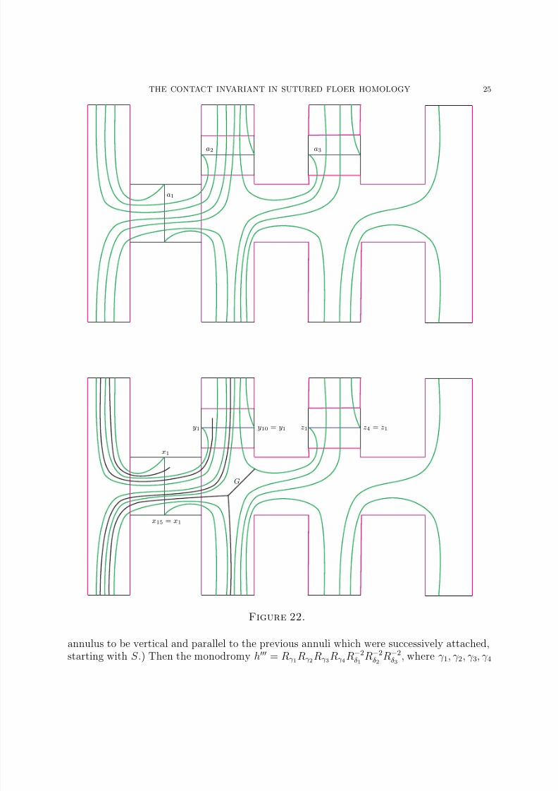
R−2δ2
, where γ 1, γ 2, γ 3 are parallel to the two boundary componentsin the middle and δ1, δ2 are the core curves of the middle vertical annuli. Let {a1, a2, a3}be the basis, ordered from left to right in Figure 22. (The arcs are on S ′′ × {−1}, whereS ′′ is the page. The α-curves are αi = ∂ (ai × [−1, 1]).) To determine whether EH = 0, weapply the Sarkar-Wang algorithm [SW] (also see [Pl]) to isotop β i so that the only regions of Σ − ∪iαi − ∪iβ i which do not intersect the suture are quadrilaterals. (Such a diagram we callcombinatorial .) Let G (in black) be the trivalent graph in the bottom diagram of Figure 22.By isotoping β 3 across G, the Heegaard diagram becomes combinatorial. Now label theintersections α1 ∩ β as x1, . . . , x14, x15 = x1 from top to bottom, α2 ∩ β as y1, . . . , y9, y10 = y1from left to right, and α3 ∩ β as z1, . . . , z4 = z1 from left to right. Observe that eachintersection of the graph with αi corresponds to two consecutive intersections with the newβ 3.
We now directly prove that EH = 0. If c1c2c3c4 is a quadrilateral which avoids the suture,and ∂ (c1, c3, y) = (c2, c4, y) + . . . (for some y), then we say that c1, c3 are the “from” cornersof the quadrilateral and c2, c4 are the “to” corners of the quadrilateral. One readily calculatesthat the only quadrilateral where the “to” corners are in {x1, y1, z1} is y1y2z1z2. Now,
∂ (x1, y2, z2) = (x1, y1, z1) + (x1, y3, z2),
where the second term comes from a bigon. Next, the only quadrilateral where the “to”corners are in {x1, y3, z2} is x1x2y3y4. We compute that
∂ (x2
, y4, z
2) = (x
1, y
3, z
2) + (x
3, y
4, z
2).
Continuing, the only quadrilateral with “to” corners in {x3, y4, z2} is x3x4z3z2. We have
∂ (x4, y4, z3) = (x3, y4, z2) + (x7, y1, z3).
There is nothing else with “to” corners in {x7, y1, z3}. Hence EH = 0.
(c) Now consider M ′′′ = T 2 × [0, 4], where #ΓT 0 = #ΓT 4 = 2, slope(ΓT 0) = slope(ΓT 4) = 0,and the contact structure ξ′′′ has “torsion” ≈ 2π. (This is the contact structure describedin the first paragraph of Example 6.) The page S ′′′ is obtained from the page S ′′ for M ′′
by attaching an annulus along the right-hand boundary in Figure 22. (We can draw the
8/3/2019 Ko Honda, William H. Kazez and Gordana Matic- The Contact Invariant in Sutured Floer Homology
http://slidepdf.com/reader/full/ko-honda-william-h-kazez-and-gordana-matic-the-contact-invariant-in-sutured 25/34
THE CONTACT INVARIANT IN SUTURED FLOER HOMOLOGY 25
a1
a2 a3
G
x1
x15 = x1
y1 y10 = y1 z1 z4 = z1
Figure 22.
annulus to be vertical and parallel to the previous annuli which were successively attached,starting with S .) Then the monodromy h′′′ = Rγ 1Rγ 2Rγ 3Rγ 4R−2
δ1R−2
δ2R−2
δ3, where γ 1, γ 2, γ 3, γ 4
8/3/2019 Ko Honda, William H. Kazez and Gordana Matic- The Contact Invariant in Sutured Floer Homology
http://slidepdf.com/reader/full/ko-honda-william-h-kazez-and-gordana-matic-the-contact-invariant-in-sutured 26/34
26 KO HONDA, WILLIAM H. KAZEZ, AND GORDANA MATIC
are parallel to the three boundary components in the middle and δ1, δ2, δ3 are the core curvesof the middle vertical annuli. One can probably directly show that EH (M ′′′, Γ′′′, ξ′′′) = 0
with some patience, but instead we invoke Theorem 4.5 and observe that (M ′′′
, ξ′′′
) canbe embedded in the unique Stein fillable contact structure on T 3, which has nonvanishingcontact invariant.
(d) Recall that a contact manifold (M, ξ) has nπ-torsion with n a positive integer if it admitsan embedding (T 2 × [0, 1], ηnπ) → (M, ξ), where (x,y,t) are coordinates on T 2 × [0, 1] ≃R2/Z2 × [0, 1] and ηnπ = ker(cos(nπt)dx − sin(nπt)dy). In a subsequent paper [GHV],Ghiggini, the first author, and Van Horn-Morris prove that if (M, ξ) has torsion ≥ 2π withM closed, then EH (M, ξ) = 0 when Z-coefficients are used.
6. Relationship with sutured manifold decompositions
A sutured manifold decomposition (M, Γ)
T
(M ′
, Γ′
) is well-groomed if for every compo-nent R of ∂M − Γ, T ∩ R is a union of parallel oriented nonseparating simple closed curves if R is nonplanar and arcs if R is planar. According to [HKM3], to each well-groomed sutured
manifold decomposition there is a corresponding convex decomposition (M, Γ)(T,ΓT ) (M ′, Γ′),
where T is a convex surface with Legendrian boundary and ΓT is a dividing set which is ∂ -parallel, i.e., each component of ΓT cuts off a half-disk which intersects no other componentof ΓT .
In [Ju2], Juhasz proved the following theorem:
Theorem 6.1 (Juhasz). Let (M, Γ)T (M ′, Γ′) be a well-groomed sutured manifold decom-
position. Then SFH (−M ′, −Γ′) is a direct summand of SFH (−M, −Γ).
More precisely, SFH (−M ′, −Γ′) is the direct sum ⊕sSFH (−M, −Γ, s), where s rangesover all relative Spinc-structures which evaluate maximally on T . (The are called “outer” in[Ju2].)
In this section we give an alternate proof from the contact-topological perspective. Weremark that our proof does not require the use of the Sarkar-Wang algorithm. In particular,our proof will imply the following:
Theorem 6.2. Let (M, Γ, ξ) be the contact structure obtained from (M ′, Γ′, ξ′) by gluing along a ∂ -parallel (T, ΓT ). Under the inclusion of SFH (−M ′, −Γ′) in SFH (−M, −Γ) as a direct summand, EH (M ′, Γ′, ξ′) is mapped to EH (M, Γ, ξ).
Corollary 6.3.EH (M
′
, Γ
′
, ξ
′
) = 0 if and only if EH (M, Γ, ξ) = 0.Proof. The “if” direction is given by Theorem 4.5. The “only if” direction follows fromTheorem 6.2.
The corollary is a gluing theorem for tight contact structures which are glued along a ∂ -parallel dividing set, and does not require any universally tight condition which was neededfor its predecessors, e.g., Colin’s gluing theorem [Co1].
Proof. Let T be a convex surface with Legendrian boundary and ΓT be its dividing set, whichwe assume is ∂ -parallel. Let (M, Γ, ξ) be a contact structure obtained from (M ′, Γ′, ξ′) by
8/3/2019 Ko Honda, William H. Kazez and Gordana Matic- The Contact Invariant in Sutured Floer Homology
http://slidepdf.com/reader/full/ko-honda-william-h-kazez-and-gordana-matic-the-contact-invariant-in-sutured 27/34
THE CONTACT INVARIANT IN SUTURED FLOER HOMOLOGY 27
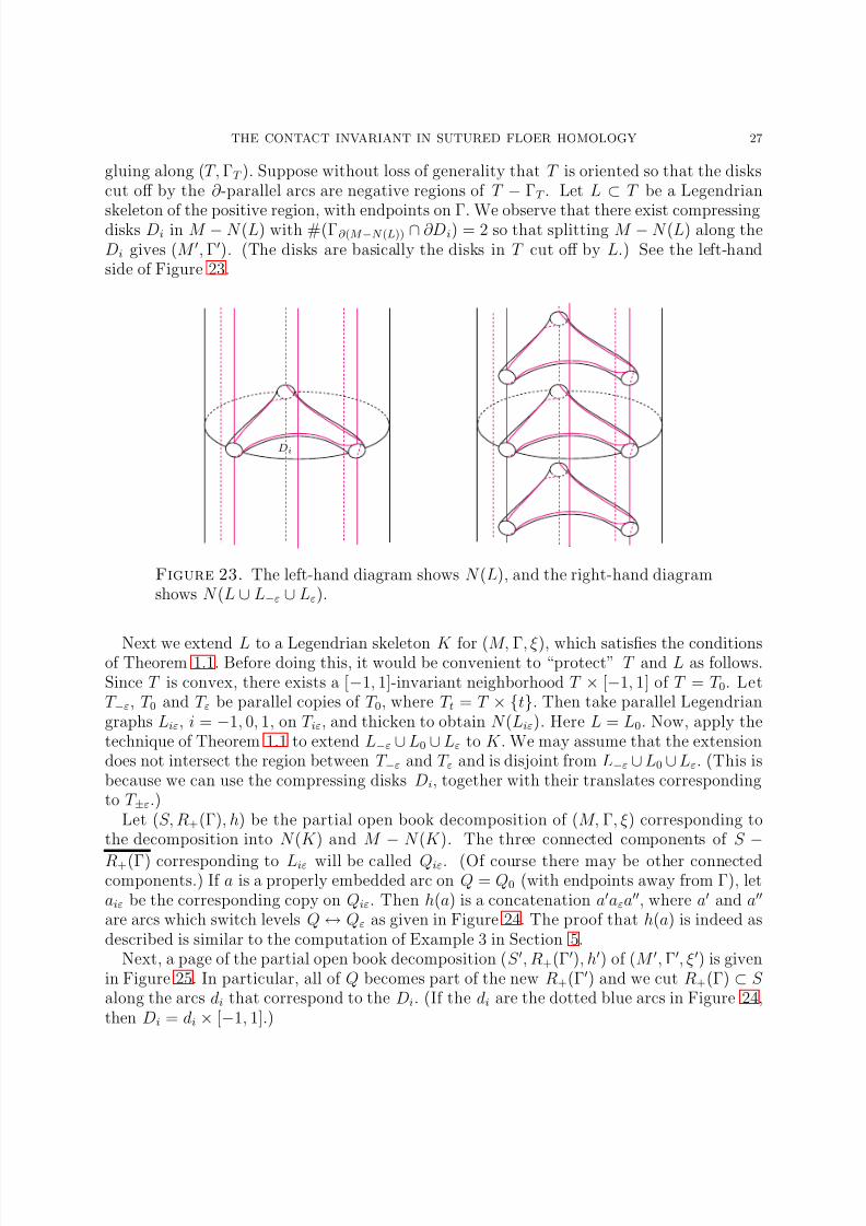
gluing along (T, ΓT ). Suppose without loss of generality that T is oriented so that the diskscut off by the ∂ -parallel arcs are negative regions of T − ΓT . Let L ⊂ T be a Legendrian
skeleton of the positive region, with endpoints on Γ. We observe that there exist compressingdisks Di in M − N (L) with #(Γ∂ (M −N (L)) ∩ ∂Di) = 2 so that splitting M − N (L) along theDi gives (M ′, Γ′). (The disks are basically the disks in T cut off by L.) See the left-handside of Figure 23.
Di
Figure 23. The left-hand diagram shows N (L), and the right-hand diagramshows N (L ∪ L−ε ∪ Lε).
Next we extend L to a Legendrian skeleton K for (M, Γ, ξ), which satisfies the conditionsof Theorem 1.1. Before doing this, it would be convenient to “protect” T and L as follows.Since T is convex, there exists a [−1, 1]-invariant neighborhood T × [−1, 1] of T = T 0. LetT −ε, T 0 and T ε be parallel copies of T 0, where T t = T × {t}. Then take parallel Legendriangraphs Liε, i = −1, 0, 1, on T iε, and thicken to obtain N (Liε). Here L = L0. Now, apply thetechnique of Theorem 1.1 to extend L−ε ∪ L0 ∪ Lε to K . We may assume that the extensiondoes not intersect the region between T −ε and T ε and is disjoint from L−ε ∪ L0 ∪ Lε. (This isbecause we can use the compressing disks Di, together with their translates correspondingto T ±ε.)
Let (S, R+(Γ), h) be the partial open book decomposition of (M, Γ, ξ) corresponding tothe decomposition into N (K ) and M − N (K ). The three connected components of S −
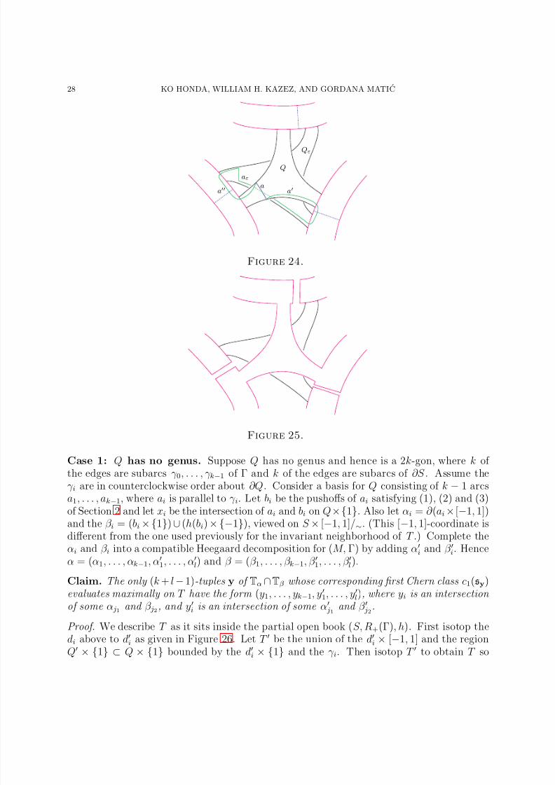
R+(Γ) corresponding to Liε will be called Qiε. (Of course there may be other connectedcomponents.) If a is a properly embedded arc on Q = Q0 (with endpoints away from Γ), letaiε be the corresponding copy on Qiε. Then h(a) is a concatenation a′aεa′′, where a′ and a′′
are arcs which switch levels Q ↔ Qε as given in Figure 24. The proof that h(a) is indeed asdescribed is similar to the computation of Example 3 in Section 5.
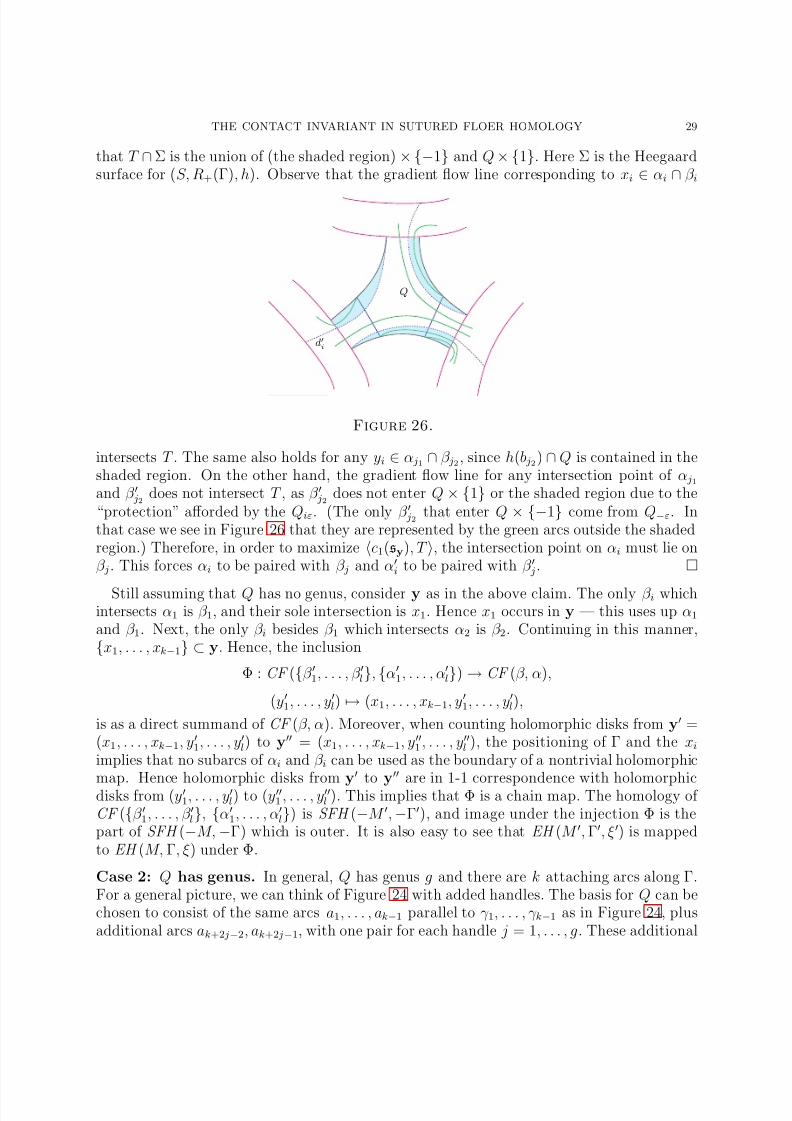
Next, a page of the partial open book decomposition (S ′, R+(Γ′), h′) of (M ′, Γ′, ξ′) is givenin Figure 25. In particular, all of Q becomes part of the new R+(Γ′) and we cut R+(Γ) ⊂ S along the arcs di that correspond to the Di. (If the di are the dotted blue arcs in Figure 24,then Di = di × [−1, 1].)
8/3/2019 Ko Honda, William H. Kazez and Gordana Matic- The Contact Invariant in Sutured Floer Homology
http://slidepdf.com/reader/full/ko-honda-william-h-kazez-and-gordana-matic-the-contact-invariant-in-sutured 28/34
28 KO HONDA, WILLIAM H. KAZEZ, AND GORDANA MATIC
Q
a
Qε
aε
a′a′′
Figure 24.
Figure 25.
Case 1: Q has no genus. Suppose Q has no genus and hence is a 2k-gon, where k of the edges are subarcs γ 0, . . . , γ k−1 of Γ and k of the edges are subarcs of ∂S . Assume theγ i are in counterclockwise order about ∂Q. Consider a basis for Q consisting of k − 1 arcsa1, . . . , ak−1, where ai is parallel to γ i. Let bi be the pushoffs of ai satisfying (1), (2) and (3)of Section 2 and let xi be the intersection of ai and bi on Q×{1}. Also let αi = ∂ (ai ×[−1, 1])and the β i = (bi × {1}) ∪ (h(bi) × {−1}), viewed on S × [−1, 1]/∼. (This [−1, 1]-coordinate isdifferent from the one used previously for the invariant neighborhood of T .) Complete the
αi and β i into a compatible Heegaard decomposition for (M, Γ) by adding α′i and β
′i. Hence
α = (α1, . . . , αk−1, α′1, . . . , α′l) and β = (β 1, . . . , β k−1, β ′1, . . . , β ′l).
Claim. The only (k + l − 1)-tuples y of Tα ∩Tβ whose corresponding first Chern class c1( sy)evaluates maximally on T have the form (y1, . . . , yk−1, y′1, . . . , y′l), where yi is an intersection of some α j1 and β j2, and y′i is an intersection of some α′
j1 and β ′ j2.
Proof. We describe T as it sits inside the partial open book (S, R+(Γ), h). First isotop thedi above to d′i as given in Figure 26. Let T ′ be the union of the d′i × [−1, 1] and the regionQ′ × {1} ⊂ Q × {1} bounded by the d′i × {1} and the γ i. Then isotop T ′ to obtain T so
8/3/2019 Ko Honda, William H. Kazez and Gordana Matic- The Contact Invariant in Sutured Floer Homology
http://slidepdf.com/reader/full/ko-honda-william-h-kazez-and-gordana-matic-the-contact-invariant-in-sutured 29/34
THE CONTACT INVARIANT IN SUTURED FLOER HOMOLOGY 29
that T ∩ Σ is the union of (the shaded region) × {−1} and Q × {1}. Here Σ is the Heegaardsurface for (S, R+(Γ), h). Observe that the gradient flow line corresponding to xi ∈ αi ∩ β i
Q
d′i
Figure 26.
intersects T . The same also holds for any yi ∈ α j1 ∩ β j2, since h(b j2) ∩ Q is contained in theshaded region. On the other hand, the gradient flow line for any intersection point of α j1
and β ′ j2 does not intersect T , as β ′ j2 does not enter Q × {1} or the shaded region due to the“protection” afforded by the Qiε. (The only β ′ j2 that enter Q × {−1} come from Q−ε. Inthat case we see in Figure 26 that they are represented by the green arcs outside the shadedregion.) Therefore, in order to maximize c1( sy), T , the intersection point on αi must lie onβ j. This forces αi to be paired with β j and α′
i to be paired with β ′ j.
Still assuming that Q has no genus, consider y as in the above claim. The only β i whichintersects α1 is β 1, and their sole intersection is x1. Hence x1 occurs in y — this uses up α1
and β 1. Next, the only β i besides β 1 which intersects α2 is β 2. Continuing in this manner,{x1, . . . , xk−1} ⊂ y. Hence, the inclusion
Φ : CF ({β ′1, . . . , β ′l}, {α′1, . . . , α′l}) → CF (β, α),
(y′1, . . . , y′l) → (x1, . . . , xk−1, y′1, . . . , y′l),
is as a direct summand of CF (β, α). Moreover, when counting holomorphic disks from y′ =(x1, . . . , xk−1, y′1, . . . , y′l) to y′′ = (x1, . . . , xk−1, y′′1 , . . . , y′′l ), the positioning of Γ and the xi
implies that no subarcs of αi and β i can be used as the boundary of a nontrivial holomorphic
map. Hence holomorphic disks fromy′
toy′′
are in 1-1 correspondence with holomorphicdisks from (y′1, . . . , y′l) to (y′′1 , . . . , y′′l ). This implies that Φ is a chain map. The homology of CF ({β ′1, . . . , β ′l}, {α′
1, . . . , α′l}) is SFH (−M ′, −Γ′), and image under the injection Φ is thepart of SFH (−M, −Γ) which is outer. It is also easy to see that EH (M ′, Γ′, ξ′) is mappedto EH (M, Γ, ξ) under Φ.
Case 2: Q has genus. In general, Q has genus g and there are k attaching arcs along Γ.For a general picture, we can think of Figure 24 with added handles. The basis for Q can bechosen to consist of the same arcs a1, . . . , ak−1 parallel to γ 1, . . . , γ k−1 as in Figure 24, plusadditional arcs ak+2 j−2, ak+2 j−1, with one pair for each handle j = 1, . . . , g. These additional
8/3/2019 Ko Honda, William H. Kazez and Gordana Matic- The Contact Invariant in Sutured Floer Homology
http://slidepdf.com/reader/full/ko-honda-william-h-kazez-and-gordana-matic-the-contact-invariant-in-sutured 30/34
30 KO HONDA, WILLIAM H. KAZEZ, AND GORDANA MATIC
1
2
3
Q
Qε
β ′
j
α′j
Figure 27.
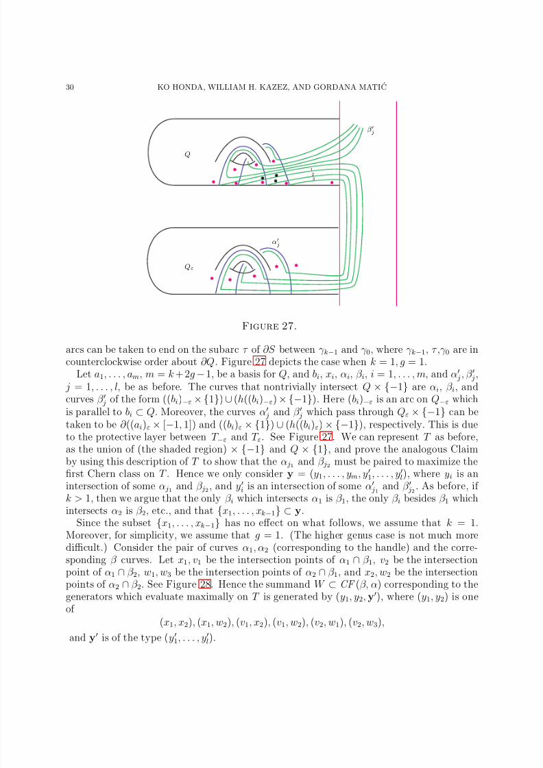
arcs can be taken to end on the subarc τ of ∂S between γ k−1 and γ 0, where γ k−1, τ ,γ 0 are incounterclockwise order about ∂Q. Figure 27 depicts the case when k = 1, g = 1.
Let a1, . . . , am, m = k + 2g − 1, be a basis for Q, and bi, xi, αi, β i, i = 1, . . . , m, and α′ j , β ′ j,
j = 1, . . . , l, be as before. The curves that nontrivially intersect Q × {−1} are αi, β i, and
curves β ′
j of the form ((bi)−ε × {1}) ∪ (h((bi)−ε) × {−1}). Here (bi)−ε is an arc on Q−ε whichis parallel to bi ⊂ Q. Moreover, the curves α′ j and β ′ j which pass through Qε × {−1} can be
taken to be ∂ ((ai)ε × [−1, 1]) and ((bi)ε × {1}) ∪ (h((bi)ε) × {−1}), respectively. This is dueto the protective layer between T −ε and T ε. See Figure 27. We can represent T as before,as the union of (the shaded region) × {−1} and Q × {1}, and prove the analogous Claimby using this description of T to show that the α j1 and β j2 must be paired to maximize thefirst Chern class on T . Hence we only consider y = (y1, . . . , ym, y′1, . . . , y′l), where yi is anintersection of some α j1 and β j2, and y′i is an intersection of some α′ j1 and β ′ j2 . As before, if k > 1, then we argue that the only β i which intersects α1 is β 1, the only β i besides β 1 whichintersects α2 is β 2, etc., and that {x1, . . . , xk−1} ⊂ y.
Since the subset {x1, . . . , xk−1} has no effect on what follows, we assume that k = 1.
Moreover, for simplicity, we assume that g = 1. (The higher genus case is not much moredifficult.) Consider the pair of curves α1, α2 (corresponding to the handle) and the corre-sponding β curves. Let x1, v1 be the intersection points of α1 ∩ β 1, v2 be the intersectionpoint of α1 ∩ β 2, w1, w3 be the intersection points of α2 ∩ β 1, and x2, w2 be the intersectionpoints of α2 ∩ β 2. See Figure 28. Hence the summand W ⊂ CF (β, α) corresponding to thegenerators which evaluate maximally on T is generated by (y1, y2, y′), where (y1, y2) is oneof
(x1, x2), (x1, w2), (v1, x2), (v1, w2), (v2, w1), (v2, w3),
and y′ is of the type (y′1, . . . , y′l).
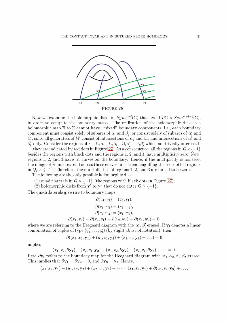
8/3/2019 Ko Honda, William H. Kazez and Gordana Matic- The Contact Invariant in Sutured Floer Homology
http://slidepdf.com/reader/full/ko-honda-william-h-kazez-and-gordana-matic-the-contact-invariant-in-sutured 31/34
THE CONTACT INVARIANT IN SUTURED FLOER HOMOLOGY 31
x1 x2 x1 x2
u1
v1
v2
w1
w2
w3
Figure 28.
Now we examine the holomorphic disks in Symm+l(Σ) that avoid ∂ Σ × Symm+l−1(Σ),in order to compute the boundary maps. The realization of the holomorphic disk as aholomorphic map u to Σ cannot have “mixed” boundary components, i.e., each boundarycomponent must consist solely of subarcs of αi and β j , or consist solely of subarcs of α′
i andβ ′ j, since all generators of W consist of intersections of α j and β k, and intersections of α′ j andβ ′k only. Consider the regions of Σ − ∪iαi − ∪iβ i − ∪ jα′
j − ∪ jβ ′ j which nontrivially intersect Γ— they are indicated by red dots in Figure 27. As a consequence, all the regions in Q×{−1}besides the regions with black dots and the regions 1, 2, and 3, have multiplicity zero. Now,regions 1, 2, and 3 have α′
j curves on the boundary. Hence, if the multiplicity is nonzero,the image of u must extend across those curves, in the end engulfing the red-dotted regions
in Qε × {−1}. Therefore, the multiplicities of regions 1, 2, and 3 are forced to be zero.The following are the only possible holomorphic disks:
(1) quadrilaterals in Q × {−1} (the regions with black dots in Figure 27);(2) holomorphic disks from y′ to y′′ that do not enter Q × {−1}.
The quadrilaterals give rise to boundary maps:
∂ (u1, v2) = (x2, v1),
∂ (v1, w2) = (v2, w1),
∂ (v2, w3) = (x1, w2),
∂ (x1, x2) = ∂ (x2, v1) = ∂ (v2, w1) = ∂ (x1, w2) = 0,
where we are referring to the Heegaard diagram with the α′i, β
′i erased. If yi denotes a linearcombination of tuples of type (y′1, . . . , y′l) (by slight abuse of notation), then
∂ ((x1, x2, y1) + (u1, v2, y2) + (x2, v1, y3) + . . . ) = 0
implies(x1, x2, ∂ y1) + (x2, v1, y2) + (u1, v2, ∂ y2) + (x2, v1, ∂ y3) + · · · = 0.
Here ∂ yi refers to the boundary map for the Heegaard diagram with α1, α2, β 1, β 2 erased.This implies that ∂ y1 = ∂ y2 = 0, and ∂ y3 = y2. Hence,
(x1, x2, y1) + (u1, v2, y2) + (x2, v1, y3) + · · · = (x1, x2, y1) + ∂ (u1, v2, y3) + . . . ,
8/3/2019 Ko Honda, William H. Kazez and Gordana Matic- The Contact Invariant in Sutured Floer Homology
http://slidepdf.com/reader/full/ko-honda-william-h-kazez-and-gordana-matic-the-contact-invariant-in-sutured 32/34
32 KO HONDA, WILLIAM H. KAZEZ, AND GORDANA MATIC
and the inclusionΦ : CF ({β ′1, . . . , β ′l}, {α′
1, . . . , α′l}) → CF (β, α),
(y′1, . . . , y′l) → (x1, x2, y′1, . . . , y′l),induces an isomorphism of SFH (−M ′, −Γ′) onto a direct summand of SFH (−M, −Γ), asbefore.
Acknowledgements. We thank Andras Juhasz for patiently explaining sutured Floer ho-mology and Andras Stipsicz for helpful discussions. We also thank John Etnyre for thediscussions which led to the reformulation of the contact invariant in [HKM2].
References
[Ba] J. Baldwin, Comultiplicativity of the Ozsv´ ath-Szab´ o contact invariant , preprint 2007.ArXiv:math.SG/0702603.
[Co1] V. Colin, Recollement de varietes de contact tendues, Bull. Soc. Math. France 127 (1999), 43–69.[Co2] V. Colin, Livres ouverts en geometrie de contact [d’apres Emmanuel Giroux] , Seminaire Bourbaki, to
appear.[Et] J. Etnyre, Lectures on open book decompositions and contact structures, in Floer homology, gauge theory,
and low-dimensional topology, 103–141, Clay Math. Proc., 5, Amer. Math. Soc., Providence, RI, 2006.[Ga] D. Gabai, Foliations and the topology of 3-manifolds, J. Differential Geom. 18 (1983), 445–503.[GHV] P. Ghiggini, K. Honda and J. Van Horn-Morris, The vanishing of the contact invariant in the presence
of torsion , preprint 2007. ArXiv:0706.1602.[Gi1] E. Giroux, Convexite en topologie de contact , Comment. Math. Helv. 66 (1991), 637–677.[Gi2] E. Giroux, Geometrie de contact: de la dimension trois vers les dimensions superieures, Proceedings of
the International Congress of Mathematicians, Vol. II (Beijing, 2002), 405–414, Higher Ed. Press, Beijing,2002.
[Gi3] E. Giroux, Structures de contact en dimension trois et bifurcations des feuilletages de surfaces, Invent.
Math. 141 (2000), 615–689.[H1] K. Honda, On the classification of tight contact structures I , Geom. Topol. 4 (2000), 309–368 (elec-
tronic).[H2] K. Honda, Gluing tight contact structures, Duke Math. J. 115 (2002), 435–478.[HKM1] K. Honda, W. Kazez and G. Matic, Right-veering diffeomorphisms of compact surfaces with bound-
ary , Invent. Math., to appear.[HKM2] K. Honda, W. Kazez and G. Matic, On the contact class in Heegaard Floer homology , preprint
2006. ArXiv:math.GT/0609734.[HKM3] K. Honda, W. Kazez and G. Matic, Convex decomposition theory , Int. Math. Res. Not. 2002, 55–88.[Ju1] A. Juhasz, Holomorphic discs and sutured manifolds, Algebr. Geom. Topol. 6 (2006), 1429–1457 (elec-
tronic).[Ju2] A. Juhasz, Floer homology and surface decompositions, preprint 2006. ArXiv:math.GT/0609779.[Li1] R. Lipshitz, A cylindrical reformulation of Heegaard Floer homology , Geom. Topol. 10 (2006), 955–1097
(electronic).[Li2] R. Lipshitz, A Heegaard Floer invariant of bordered three-manifolds, Ph.D. thesis, 2006.[LOSS] P. Lisca, P. Ozsvath, A. Stipsicz and Z. Szabo, Heegaard Floer invariants of Legendrian knots in
contact 3-manifolds, in preparation.[OS1] P. Ozsvath and Z. Szabo, Holomorphic disks and topological invariants for closed three-manifolds,
Ann. of Math. (2) 159 (2004), 1027–1158.[OS2] P. Ozsvath and Z. Szabo, Holomorphic disks and three-manifold invariants: properties and applica-
tions, Ann. of Math. (2) 159 (2004), 1159–1245.[OS3] P. Ozsvath and Z. Szabo, Heegaard Floer homology and contact structures, Duke Math. J. 129 (2005),
39–61.
8/3/2019 Ko Honda, William H. Kazez and Gordana Matic- The Contact Invariant in Sutured Floer Homology
http://slidepdf.com/reader/full/ko-honda-william-h-kazez-and-gordana-matic-the-contact-invariant-in-sutured 33/34
THE CONTACT INVARIANT IN SUTURED FLOER HOMOLOGY 33
[OS4] P. Ozsvath and Z. Szabo, Link Floer homology and the Thurston norm , preprint 2006.ArXiv:math.GT/0601618.
[OS5] P. Ozsvath and Z. Szabo, Holomorphic triangles and invariants for smooth four-manifolds, Adv. Math.202 (2006), 326–400.
[OST] P. Ozsvath, Z. Szabo and D. Thurston, Legendrian knots, transverse knots and combinatorial Floer homology , preprint 2006. ArXiv:math.GT/0611841.
[Pl] O. Plamenevskaya, A combinatorial description of the Heegaard Floer contact invariant , preprint 2006.ArXiv:math.GT/0612322.
[SW] S. Sarkar, J. Wang, A combinatorial description of some Heegaard Floer homologies, preprint 2006.ArXiv:math.GT/0607777.
[VH] J. Van Horn-Morris, Ph.D. thesis, 2007.
University of Southern California, Los Angeles, CA 90089
E-mail address: [email protected]
URL: http://rcf.usc.edu/~khonda
University of Georgia, Athens, GA 30602E-mail address: [email protected]
URL: http://www.math.uga.edu/~will
University of Georgia, Athens, GA 30602
E-mail address: [email protected]
URL: http://www.math.uga.edu/~gordana
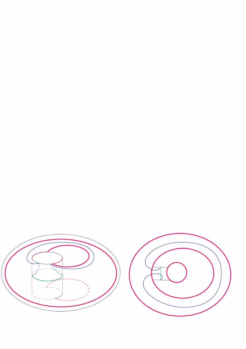
8/3/2019 Ko Honda, William H. Kazez and Gordana Matic- The Contact Invariant in Sutured Floer Homology
http://slidepdf.com/reader/full/ko-honda-william-h-kazez-and-gordana-matic-the-contact-invariant-in-sutured 34/34


![Contents - i2m.univ-amu.fr€¦ · of these invariants: an invariant of sutured 3-manifolds, due to Juh asz, called sutured Floer homology [Juh06]. The main goal will be to relate](https://img.pdfslide.us/doc/110x75/6034f152a197e573c26181a1/contents-i2muniv-amufr-of-these-invariants-an-invariant-of-sutured-3-manifolds.jpg)


![Contents · of these invariants: an invariant of sutured 3-manifolds, due to Juh asz, called sutured Floer homology [Juh06]. The main goal will be to relate these invariants to ideas](https://img.pdfslide.us/doc/110x75/5f7a9bc74e54ad20214d4968/contents-of-these-invariants-an-invariant-of-sutured-3-manifolds-due-to-juh-asz.jpg)