Embed Size (px)
Citation preview

KNOWLEDGE INSTITUTE OF TECHNOLOGY
KIOT Campus, NH – 47, Kakapalayam,
Salem – 637 504
DEPARTMENT OF CIVIL ENGINEERING
CE8461- HYDRAULIC ENGINEERING LABORATORY
2017 Regulation
IV Semester B.E. Civil Engineering
LAB MANUAL

KNOWLEDGE INSTITUTE OF TECHNOLOGY
[AFFILIATED TO ANNA UNIVERSITY, CHENNAI -600025]
KAKKAPALYAM (PO), SALEM-637504
LABORATORY MANUAL
NAME OF THE STUDENT :
REG. NO. :
YEAR / SEM :
SUBJECT CODE : CE 8461
SUBJECT NAME : HYDRAULIC ENGINEERING LABORATORY

GENERAL INSTRUCTIONS
The following instructions should be strictly followed by students in the Laboratory:
1. Students should wear lab coat in the laboratory.
2. Students are advised to enter the lab WITH FORMAL SHOES ONLY.
3. They are not supposed to operate the instrument in absents of professor/NTS.
4. They can also utilizes the laboratory during their free hours.
5. Students are advised to complete their record work before the next class.
6. Students are asked to switch off the instrument and fans before leaving the lab.
7. Students can access the instrument through lab technician.
8. Students have free access to use the instrument available in the lab.
9. During the laboratory hours, using mobile is strictly prohibited.
10. NON WATER Proof electronic things are strictly prohibited in the lab.

CE8461 - HYDRAULIC ENGINEERING LABORATORY L T P C 0 0 4 2
OBJECTIVE: Students should be able to verify the principles studied in theory by performing the experiments in lab.
LIST OF EXPERIMENTSA. Flow Measurement1. Calibration of Rotameter2. Calibration of Venturimeter / Orificemeter3. Bernoulli’s Experiment
B.Losses in Pipes4.Determination of friction factor in pipes5. Determination of min or lossesC. Pumps6. Characteristics of Centrifugal pumps7. Characteristics of Gear pump8. Characteristics of Submersible pump9. Characteristics of Reciprocating pump
D. Turbines10. Characteristics of Pelton wheel turbine11. Characteristics of Francis turbine/Kaplan turbineE. Determination of Metacentric height12.Determination of Metacentric height of floating bodies
TOTAL: 60 PERIODSOUTCOMES:
The students will be able to measure flow in pipes and determine frictional losses. The students will be able to develop characteristics of pumps and turbines.
REFERENCES:1. Sarbjit Singh."Experiments in Fluid Mechanics", Prentice Hall of India Pvt. Ltd, Learning Private
Limited, Delhi, 2009.2. "Hydraulic Laboratory Manual", Centre for Water Resources, Anna University, 2004.3. Modi P.N. and Seth S.M., "Hydraulics and Fluid Mechanics", Standard Book House, New Delhi, 2000.4. Subramanya K. "Flow in open channels", Tata McGraw Hill Publishing.Company, 2001.
LIST OF EQUIPMENTS1. One set up of Rotometer2. One set up of Venturimeter/Orifice meter3. One Bernoulli’s Experiment set up4. One set up of Centrifugal Pump5. One set up of Gear Pump6. One set up of Submersible pump7. One set up of Reciprocating Pump8. One set up of Pelton Wheel turbine9. One set up of Francis turbines/one set of kaplon turbine10. One set up of equipment for determination of Metacentric height of floating bodies11. One set up for determination of friction factor in pipes12. One set up for determination of minor losses.

INDEX
S. No Date Name of the Experiment Marks Sign
1. Calibration of Rotameter
2. Calibration of Venturimeter / Orificemeter
3. Bernoulli’s Experiment
4. Determination of friction factor in pipes
5. Determination of min or losses
6. Characteristics of Centrifugal pumps
7. Characteristics of Gear pump
8. Characteristics of Submersible pump
9. Characteristics of Reciprocating pump
10. Characteristics of Pelton wheel turbine
11. Characteristics of Francis turbine/Kaplan turbine
12. Determination of Metacentric height of floating bodies

1
TABULATION
Internal area of measuring tank (A) = 300mm x 300mm
Difference in level of water (h) = 50mm
S. No Rota meter
reading (lpm)
Time taken (t) for H=50 mm rise in collecting tank (sec)
Actual Discharge
(m3/sec)
Actual
discharge
(lit/sec)
Percentage
Error of Rota
meter (%) T1 T2 Mean
Mean

2
AIM
To determine the percentage error in Rota meter with the actual flow rate.
APPARATUS REQUIRED
1. Rotameter (0–10LPMrange)
2. Single phase mono block pump set (0.5HP, 1440RPM)
3. Reservoir tank arrangement.
4. Measuring tank arrangement.
5. Piping System
FORMULAE
ACTUAL DISCHARGE
Actual rate of flow Qact = 𝐴𝐻
𝑡 mm3/sec
Where A = Area of the measuring tank in mm2.
h = Difference in levels of water in mm
t = Time taken for 5 cm rise of water level in collecting Tank in Seconds.
CONVERSION
Flow rate conversion:
Amount: 1 cubic millimeter per second (mm3/sec) of flow rate.
Equals: 0.000060 liters per minute (litre/min) in flow rate.
Converting cubic meter per second to liters per minute value in the flow rate units scale.
Actual flow rate (lit/sec), Qact = Qact x 0.000060 (litre/min)
Percentage error of Rota meter (%) = 𝐴𝑐𝑡𝑢𝑎𝑙 𝐷𝑖𝑠𝑐ℎ𝑎𝑟𝑔𝑒 −𝑅𝑜𝑡𝑎𝑚𝑒𝑡𝑒𝑟 𝑟𝑒𝑎𝑑𝑖𝑛𝑔
𝑅𝑜𝑡𝑎𝑚𝑒𝑡𝑒𝑟 𝑟𝑒𝑎𝑑𝑖𝑛𝑔×100
Ex.No: 1
Date: CALIBRATION OF ROTAMETER

3

4
PROCEDURE
1. Switch on the motor and the delivery valve is opened.
2. Adjust the delivery valve to control the rate in the pipe.
3. Set the flow rate in the Rota meter, for example say 50 liters per minute
4. Note down the time taken for 5cm rise in collecting tank
5. Repeat the experiment for different set of Rota meter readings
6. Tabular column is drawn and readings are noted
7. Graphic drawn by plotting Rota meter reading Vs percentage error of the Rota meter
GRAPH:
Rota meter reading Vs percentage error
RESULT The percentage error of the Rota meter was found to be ……………
5
EXPERIMENTAL SET-UP:
The set-up consists of a pipe connected to a constant head supply tank. A horizontal
Venturimeter is fitted to the pipe at a distance of an atleast 30 times diameter. A regulating
valve is provided at the exit to vary the discharge as shown in figure. A measuring tank is
provided to determine the discharge. The difference of pressure between the inlet and the throat
is measured with U- tube manometer.
Theoretical Discharge , (Qt)
(Qt) =a1a2√2gh
√a12 − a2
2 (mm3/sec)
Where,
a1= Area of inlet pipe in mm2.
a2= Area of throat in mm2.
h = the pressure difference in mm.
The pressure difference h is determined from the deflection of the manometer liquid (h).
Thus
h = (h1 − h2) (Sm
Sl
− 1) (mm)
Where
h1 = Manometric head in one limb of the manometer in mm.
h2 = Manometric head in other limb of the manometer in mm.
Sm = specific gravity of the manometer liquid in mm.
Sl = specific gravity of the fluid in the pipe.
g = Acceleration due to gravity in mm/sec2.
Actual Discharge
(Qa ) =Internal plan area of collecting tank(A) ×Rise of liquid (H)
Time of collection (t) =
AH
t (mm3 /sec)
Coefficient of discharge, Cd
Cd =Qa
Qt
(𝑁𝑜 𝑢𝑛𝑖𝑡)

6
AIM:
To determine the coefficient of discharge (Cd) of a given Venturimeter.
APPARATUS USED:
A Venturimeter
Differential U –tube manometer
Meter Scale
Stop watch
Collecting tank, fitted with piezometer and control valve.
INTRODUCTION:
1. A Venturimeter is commonly used to measure discharge in closed conduits having pipe
flow. It consists of a converging cone, a throat section and a diverging cone. An expression
for the discharge is derived by applying the Bernoulli equation to the inlet and the throat
and using the continuity equation. The discharge
Q = Cd
a1a2
√a12 − a2
2√2gh (mm3/sec)
Where
Cd = coefficient of discharge, between 0.97 to 0.99
a1 = area of cross section at the inlet in mm2
a2 = area of cross section at the throat in mm2
h = difference of piezometric heads in mm
2. The converging cone has an angle of convergence about 20°. The flow in the converging
cone is accelerating and the loss of head is relatively small.
3. The diverging cone, the flow is decelerating. To avoid excessive head loss, it is essential to
keep the angle of divergence small, usually 5° to 7°.
4. Throat diameter D2 is between ¼ to ¾ times the inlet diameters D1. The smaller the D2/ D1
ratio, the more is the pressure difference. However, the pressure at the throat should not be
allowed to drop to the vapour pressure to prevent cavitations.
5. For accurate results, the Venturimeter should be preceded by a straight and uniform length
of about 30D1 or so. Alternatively, straightening vanes can be used in the pipe.
Ex.No: 2
Date: FLOW THROUGH VENTURIMETER

7
OBSERVATION AND CALCULATION:
Acceleration due to gravity, g = 9810 mm/sec2 Area of the pipe 1-1 (a1) = 490.87 mm2
Diameter of inlet, D1 = 25 mm Area of the pipe 1-1 (a2)= 176.71 mm2
Diameter of inlet, D2 = 15 mm Area of the collecting tank (A) = 250000 mm2
Internal plan dimension, L = 500 mm Specific gravity of mercury, (Sm) = 13.6
B = 500 mm Specific gravity, (Sl) = 1
S.No Manometric
readings
( mm of mercury)
h = (h1 − h2)
(Sm
Sl− 1)
(mm)
√h
(mm)
Time taken ‘t’ for H=50 mm
rise in collecting tank (sec)
Discharge in
mm3/sec
Coefficient of
discharge
Cd =Qa
Qt
h1 h2 h1- h2 T1 T2 Avg Qa=
AH
t Qt
=a1a2√2gh
√a12 − a2
2
Mean value of Cd
8
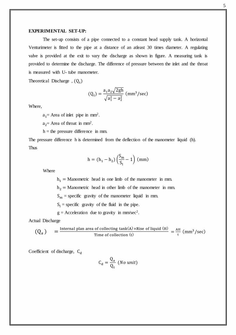
PROCEDURE:
1. Measure the inlet and throat diameters of the Venturimeter. Also measure the length
and width of the measuring tank.
2. Keep the outlet valve closed and the inlet valve is opened fully.
3. The outlet valve is opened slightly and the manometric heads is both the limbs (h1 and
h2) are noted. Measure the deflection of the manometer liquid.
4. The outlet valve of the collecting tank is closed tightly and the time ‘t' and required for
H rise of water in the collecting tank is observed using a stopwatch. Collect water in
the measuring tank for a suitable time period.
5. Repeat step 2 and 4 for different discharges. The observation are tabulated and the
coefficient and orifice meter cd i.e. computed.
Graphs:
Plot a graph between Q and h on an ordinary graph paper, with Q as ordinate. Measure the
slope of the straight line and hence determine the coefficient of discharge.
Result:
Coefficient of dischargeCd (Analytically) =
Coefficient of discharge Cd (Graphically) =

9
Formulae:
1. Theoretical Discharge of orifice meter
𝑄𝑡ℎ =𝑎1𝑎2√2𝑔ℎ
√𝑎12−𝑎2
2 (mm3/sec)
Where
= Theoretical Discharge in mm3/sec.
a1 = Area of inlet in mm2.
a2 = Area of orifice in mm2.
g = Acceleration due to gravity in mm/sec2.
h = Orifice head in terms of following liquid in mm.
h = (h1 – h2)
h1 = Manometric head in one limb of the manometer in mm.
h2 = Manometric head in other limb of the manometer in mm.
2. Actual Discharge
= (mm3/sec)
Where,
A = internal plan area of collecting tank in mm2.
H = Rise of liquid in mm.
T = time of collection in sec.
3. Coefficient of Discharge
Coefficient of orifice meter ( is the ratio between the actual discharge (Qa)
and the theoretical discharge (Qt)
Cd =Qa
Qt
(𝑁𝑜 𝑢𝑛𝑖𝑡)
Qa = Actual discharge in mm3/sec.
Qt = Theoretical discharge in mm3/sec.

10
AIM:
To determine the coefficient of discharge (Cd) of the given orifice meter.
APPARATUS USED:
1. Orifice meter with all accessories
2. Meter Scale
3. Stop watch
4. Collecting tank, fitted with control valve.
INTRODUCTION:
An orifice is an opening in the side wall of a tank or a vessel. The liquid flows out of
the tank when the orifice is opened. In a sharp-edged orifice, there is a line contact of the liquid
as it flows out. An orifice is called the orifice discharging free when it discharges into
atmosphere. The jet issuing from the tank forms the vena contracta at a distance of d 2⁄ , where
is the diameter of the orifice.
Discharge by Bernoulli’s theorem,
(mm3/sec)
Where,
= coefficient of contraction, varies between 0.61 and 0.65
= coefficient of velocity varies between 0.95 and 0.99
= coefficient of discharge varies between 0.59 and 0.64
= head causing flow. This is equal to the ratio vertical distance between the
free surface in the tank and the centre of the orifice in mm.
= area of the orifice of diameter in mm2.
THEORY:
Orifice meter is a device used to measure the discharge or any liquid flowing through
pipeline. The pressure difference between the inlet orifice meter is recorded using a differential
manometer the line time is recorded for a measurement discharge.
Ex.No: 3
Date: FLOW THROUGH ORIFICE METER

11
OBSERVATIONS AND CALCULATIONS:
Acceleration due to gravity = 9810 mm/sec2 Area of the pipe 1-1 (a1) = 490.87 mm2
Diameter of inlet, D1 = 25 mm Area of the pipe 1-1 (a2) = 176.71 mm2
Diameter of inlet, D2 = 15 mm Area of the collecting Tank (A) = 250000 mm2
Internal plan dimension,
Length (L) = 500 mm Specific gravity of mercury (Sm) = 13.6
Breadth (B) = 500 mm Specific gravity of water (Sl)= 1
S.No
Manometer reading
Total Head
x10 (mm)
(mm)
Time taken ‘t’ for H=50 mm
rise in collecting tank (sec)
Discharge ( )
Coefficient of
discharge
Cd
Actual
Discharge
Theoretical
Discharge
h1
(cm)
h2
(cm)
X= h1 -
h2 (cm) T1 T2
Average
(sec)
𝑄𝑎
𝑄𝑡
Mean value of Cd=

12
PROCEDURE:
1. The dimensions of the inlet and orifice are recorded and the internal plan dimensions
of the collecting tank are measured.
2. Keeping the outlet valve closed, the inlet valve is opened fully.
3. The outlet valve is opened slightly and the Manometric heads in both limbs (h1 and h2)
are noted.
4. The outlet valve is the collecting tank is closed tightly and time is closed tightly and
time required for H rise of water is the collecting tank is observed using a stop watch.
5. The above procedure is repeated by gradually increasing the flow and observing the
required reading.
6. The observations are tabulated and the coefficient of orifice meterCd is computed.
GRAPH:
Plot versus on an ordinary graph, with a ordinate, and determine the value of
from the slope of the line.
RESULTS:
Coefficient of discharge of the orifice meter
1. (Analytically =
2. (Graphically) =

13
OBSERVATION:
Internal Plan Dimensions of collecting tank ,Length (L) = 300 mm
Breadth = 300 mm
a1= 50x 25mm a2= 45x25mm a3= 36x25mm a4= 25x 25mm a5= 16x25mm
a6=12.5x25mm a7= 14x25mm a8= 18.5x25mm a9=23x25mm a10= 29x25mm
a11= 36x25mm a12=41x25mm a13= 46x25mm a14= 50x 25mm
S.No Cross
section
area
Time taken
‘t’ for H=50
mm rise in
collecting
tank (sec)
Discharge
Q = 𝐀𝐇
𝐭
(mm3/sec)
Velocity
V = 𝑄
𝑎
(mm)
Velocity
head
𝑣2
2𝑔
(mm)
Piezometer
reading
h = 𝑝
𝛾
(mm)
Datum
head
Z
(mm)
Total
head
H = Z
+ 𝑃
𝛿
+𝑉2
2𝑔
(mm)
mm2 1 2 Avg
1. a1
2. a2
3. a3
4. a4
5. a5
6. a6
7. a7
8. a8
9. a9
10. a10
11. a11
12. a12
13. a13
14. a14

14
AIM
To verify the Bernoulli’s theorem Flow through variable Duct Area.
APPARATUS USED
1) A supply tank of water a tapered inclined pipe fitted with no of piezometer tubes point,
2) Measuring tank
3) Scale,
4) Stopwatch.
THEORY Bernoulli’s theorem states that when there is a continues connection between the particle of
flowing mass liquid, the total energy of any sector of flow will remain same provided there is no
reduction or addition at any point.
FORMULA
Total Head
H1 = Z1 + 𝑃
𝛿 +
𝑉2
2𝑔 (mm)
H2 = Z2 + 𝑃
𝛿 +
𝑉2
2𝑔 (mm)
Z = Datum Head (mm) 𝑃
𝛿 = Pressure Head (mm)
𝑉2
2𝑔 = Velocity Head (mm)
H = Total Head (mm)
Ex.No: 4
Date: FLOW THROUGH VARIABLE DUCT AREA-BERNOULLI’S EXPERIMENT

15

16
PROCEDURE
1. Open the inlet valve slowly and allow the water to flow from the supply tank.
2. Now adjust the flow to get a constant head in the supply tank to make flow in and outflow equal.
3. Under this condition the pressure head will become constant in the piezometer tubes.
4. Note down the quantity of water collected in the measuring tank for a given interval of time.
5. Compute the area of cross-section under the piezometer tube.
6. Compute the area of cross-section under the tube.
7. Change the inlet and outlet supply and note the reading.
8. Take at least three readings as described in the above steps.
RESULT
1. When fluid is flowing, there is a fluctuation in the height of piezometer tubes, note the mean position
carefully.
2. Carefully keep some level of fluid in inlet and outlet supply tank.

17
DESCRIPTION
The experiment is performed by using a number of long horizontal pipes of different
diameters connected to water supply using a regulator valve for achieving different constant
flow rates. Pressure tappings are provided on each pipe at suitable distances apart and
connected to U-tube differential manometer. Manometer is filled with enough mercury to read
the differential head ‘hm’. Water is collected in the collecting tank for arriving actual discharge
using stop watch and the piezometric level attached to the collecting tank.
FORMULAE USED:
1). Darcy coefficient of friction (Friction factor)
𝑓 =2𝑔 × 𝐷 × ℎ𝑓
4𝐿𝑉2
Where,
f = Darcy coefficient of friction.
g = gravity due to acceleration in mm/sec2.
D = Diameter of the pipe in mm.
hf = hm x (
m-1) (hm is differential level of manometer fluid measured in mm)
L = Length of pipe between the sections used for measuring loss of head in mm.
Qa = Actual discharge measured from volumetric technique in mm3/sec.
2. Velocity, V = Qa
a (mm/sec)
3. Actual discharge, Qa= AH
t (mm3/sec)

18
AIM:
To determine the coefficient of friction (f) of the given pipe material.
APPARATUS REQUIRED:
1. A pipe provided with inlet and outlet valves
2. U- tube manometer
3. Collecting tank
4. Stop watch
5. Meter scale
THEORY:
When liquid flows through a pipe line, it is subjected to frictional resistance. The
frictional resistance depends upon the roughness of the inner surface of the pipe. The loss of
head between selected lengths of pipe is observed for a measured discharge. The coefficient of
friction is calculated by using the expression.
hf =4fL𝑉2
2gd (mm)
Where,
fh Loss of head due to friction in mm.
L = Length of pipe between the sections used for measuring loss of head in mm.
D = Diameter of the pipe in mm.
f = Darcy coefficient of friction.
g = gravity due to acceleration in mm/sec2.
h1 = manometric head in one limb of the manometer in mm.
h2 = manometric head in outer limb of the manometer in mm.
L = length of the pipe between pressure tapping cock’s in mm.
V = velocity of flow in the pipe Qa in mm/sec.
Qa = Actual discharge in mm3/sec.
A = internal plan area of the collecting tank in mm2.
H = height of collecting on the collecting tank in mm2.
T = time of the collection in sec.
a = across sectional area of the pipe in mm2.
d = diameter of pipe in mm.
g = acceleration due to gravity in mm/sec2.
Ex.No: 5 Date: FLOW THROUGH PIPES (MAJOR LOSS)

19
Observation
Diameter of the pipe (D) = 25 mm Area of the pipe (a) = 490.625 mm2
Length of the pipe = 3000 mm Area of collecting Tank (A) = 250 x 103mm2
Length of the tank (L) = 500 mm
Breadth of the tank(b) = 500 mm
Acceleration due to gravity (g) = 9810 mm/sec2
S.No
Manometric readings Time taken ‘t’
for H=50 mm
rise in collecting
tank (sec)
Actual discharge
𝐐𝐚
(𝒎𝒎𝟑
𝑺𝒆𝒄)
Velocity
(V)
(𝒎𝒎
𝑺𝒆𝒄)
(V2)
(𝒎𝒎
𝑺𝒆𝒄)2
Coefficient of
friction
24
..2
LV
hDgf
f
h1
(mm)
h2
(mm)
hf =h1- h2
(mm)
Mean value of 𝐂𝐝

20
PROCEDURE:
1. The diameter of the pipe, the internal plane dimension of the collecting tank and the length
of the pipe line between the pressure tapping cocks are measured.
2. Keep the outlet valve fully closed, the inlet valve is opened completely.
3. The outlet valve of the collecting tank is closed tightly and the time‘t’ required for H rise
of water in the collecting tank is observed using a stop watch.
4. The above procedure is repeated by gradually increasing the flow and observing the
required readings.
5. The observations are tabulated and the coefficient of friction is computed
GRAPH:
A graph hf vs. v2 is drawn taking v2 on x axis
RESULTS
The coefficient of friction of the given pipe.
1. Theoretically f =
2. Graphically f =

21

22
AIM:
To determine the loss of coefficient of flow through pipe due to sudden enlargement,
sudden contraction, pipe fitting such as elbows, bends & etc.
APPARATUS REQUIRED:
1. Collecting tank
2. Stop watch
3. Meter scale
4. A pipe line provided with bend, elbow, pipe fitting, etc.
THEORY:
1. The loss of energy due to friction is clarified as major losses and minor losses of energy.
2. Due to charge in velocity of fluid of fluid either in magnitude described in minor
velocity.
3. In long pipes minor losses are quite small which is normally ignored however in short
that loss may be some time used weight the major losses.
4. The general equations for minor loss is,
k =2gh
V2
h1 =kV2
2g (mm)
Actual discharge
Qa= AH
t mm3/sec
V1 = Qact
a1 (mm/sec)
Where,
h1 = head losses in mm.
V = velocity of fluid flowing through normal diameter in pipe in mm/sec.
K = loss of coefficient of pipe fitting and nature of change in velocity.
PROCEDURE:
1. Select the required pipe line and noted down the diameter.
2. Connect pressure tapings in any pipe line close all other pressure tappings.
3. Open the inlet valve in selected pipe line and closed valve in remaining pipe line.
4. Open the main gate valve and connect pressure taping of the bent to the manometer.
Ex.No: 6 Date: DETERMINATION OF MINOR LOSSES
23
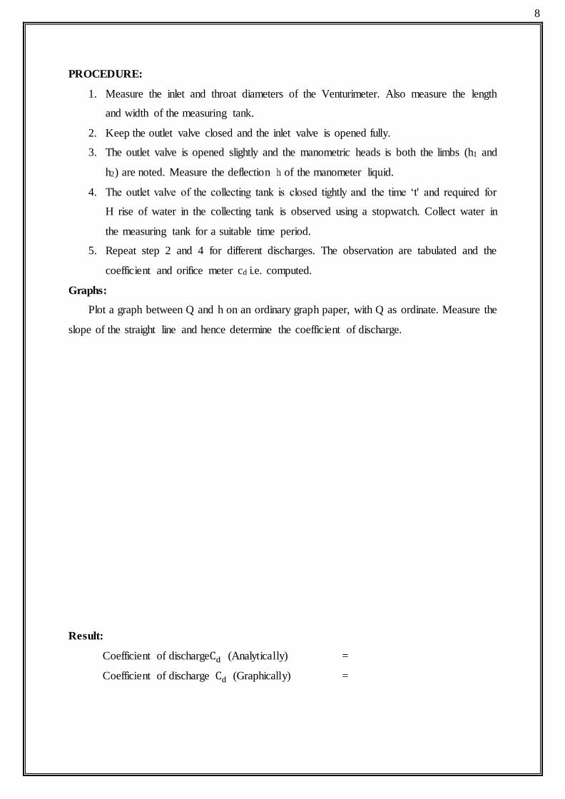
OBSERVATION
1. Loss of head due to expansion:
Dia of the pipe (d1) = 15 mm area (a1) = π/4 x 152 = 176.71 mm2
Dia of the pipe (d2) = 50 mm area (a2) = π/4 x 502 = 1963.5 mm2
Rise of water level (h) = 50 mm Area of collecting tank (A) = 160 x 106 mm2
S.No Manometer reading (H)
Time taken ‘t’ for H=50 mm rise in
collecting tank (sec)
Actual discharge
Qa= AH
t
(mm3/s)
V1 = Qact
a1
(mm/sec)
V2 = Qact
a2
(mm/sec)
Coefficient of discharge
k =2gh
(V1−V2 )2 h1
(mm)
h2
(mm)
x = h1 – h2
(mm)
24
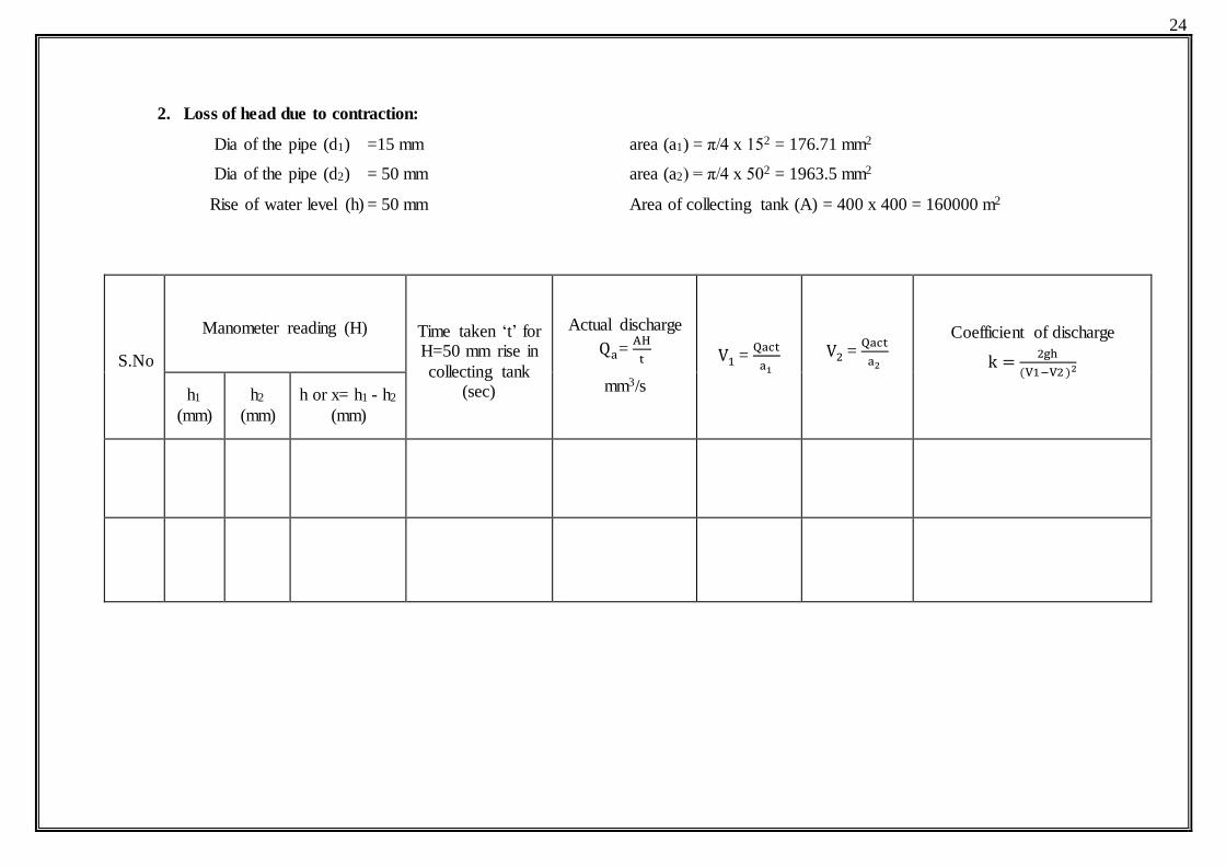
2. Loss of head due to contraction:
Dia of the pipe (d1) =15 mm area (a1) = π/4 x 152 = 176.71 mm2
Dia of the pipe (d2) = 50 mm area (a2) = π/4 x 502 = 1963.5 mm2
Rise of water level (h) = 50 mm Area of collecting tank (A) = 400 x 400 = 160000 m2
S.No
Manometer reading (H) Time taken ‘t’ for H=50 mm rise in
collecting tank (sec)
Actual discharge
Qa= AH
t
mm3/s
V1 = Qact
a1 V2 =
Qact
a2
Coefficient of discharge
k =2gh
(V1−V2 )2
h1
(mm)
h2
(mm)
h or x= h1 - h2
(mm)

25
3. Loss of head due to elbow:
Dia of the pipe (d) = 15 mm
Rise of water level (h) = 50 mm
Area of collecting tank (A) = 160000mm2
Area (a) = π/4 x 152 = 176.71 mm2
S.No
Manometer reading (H) Time taken ‘t’ for H=50 mm rise in collecting tank
(sec)
Actual discharge
Qa= AH
t
(mm3/s)
V = Qact
a1
(mm/sec)
Coefficient of discharge
k =2gh
(V)2
h1
(mm)
h2
(mm)
X= h1 – h2
(mm)

26
4. Loss of head due to bend:
Dia of the pipe (d) = 15 mm
Rise of water level (h) = 50 mm
Area of collecting tank (A) = 160000 mm2
Area (a) = π/4 x 152 = 176.71 mm2
S.No
Manometer reading (H) Time taken ‘t’ for
H=50 mm rise in collecting tank
(sec)
Actual discharge
Qa= AH
t
(mm3/s)
V = Qact
a1
(mm/sec)
Coefficient of discharge
k =2gh
(V)2
h1
(mm)
h2
(mm)
X= h1 – h2
(mm)

27
28
5. Note down the reading in left and right column of manometer.
6. Close the valve in collecting tank and note down the time taken for the h cm rise in
collecting tank.
7. Repeat the experiment for 5 set reading for different flow rate.
8. Remove and connect the pressure tapings to other pipe fittings and repeat the above
process.
RESULT
1. Loss of head due to expansion, k =
2. Loss of head due to contraction, k =
3. Loss of head due to elbow, k =
4. Loss of head due to bend, k =

29
FORMULA:
1. Total head,
H = Hs + Hd + X (m of water)
Where
Pd = Pressure head in kg cm2⁄
PV = Vacuum head in mm Hg
X = Distance between pressure gauge and vacuum gauge.
Hs = Suction head in m = [PV × 0.0136]
Hd = Delivery head in m = [Pd × 10]
2. Actual discharge, Qa =AH
t(m3 sec⁄ )
Where,
A = area of collecting tank in m2.
H = rise of water level in collecting tank = 0.05 m.
t = time taken for 5 cm rise in collecting tank in sec.
3. Input power, Pi = [3600 x (𝑛𝑟
𝑐𝑡)] (watts)
Where,
Nr = Number of revolutions of energy meter disc = 5 rev
C = Energy meter constent = 0.75
T = time for 5 revolutions energy meter disc in sec .
EMC = Energy meter constant in rev kwhr.⁄
4. Output power, PO = W × Qact × H (watts)
Where,
W = Specific weight of water 980 or 1000 (N m3⁄ )
Qa = Actual discharge in m3/sec
H = Head of water in m.
5. Efficiency of the pump, η = [Output power
Input power] × 100 (%)
ƞ 𝛈 = [PO
Pi
] × 100 (%)
30
AIM:
To study the characteristics of a centrifugal pump and to draw the characteristics
curve.
APPARATUS REQUIRED:
1. Centrifugal pump setup
2. Centrifugal pump with pressure gauge and vacuum gauge setup.
3. Stop Watch
4. Collecting tank
5. Steel Scale
THEORY:
A centrifugal pump is a roto dynamic pump that uses a rotating impeller to increase the
pressure of a fluid. The pump works by the conversion of the rotational kinetic energy, typically
from an electric motor or turbine, to an increased static fluid pressure. This action is described
by Bernoulli's principle.
The rotation of the pump impeller imparts kinetic energy to the fluid as it is drawn in
from the impeller eye and is forced outward through the impeller vanes to the periphery. As
the fluid exits the impeller, the fluid kinetic energy is then converted to pressure due to the
change in area the fluid experiences in the volute section. The energy conversion, results in an
increased pressure on the delivery side of the pump, causes the flow.
DESCRIPTION:
The test pump is a single stage centrifugal pump. It is coupled with an electric motor by
means cone pulley belt drive system. An energy meter is permanently connected to measure
the energy consumed by the electric motor for driving the pump. A stop watch is provided to
measure the input power to the pump. A pressure gauge and a vacuum gauge are fitted it the
delivery and suction pipes, respectively, to measure the pressure.
1. The pump is run by a single phase motor.
2. The pressure gauge is fitted to the delivery side and a vacuum gauge to the suction side.
3. The energy input to the pump can be measured through an energy meter.
4. There is a collecting tank with a level indicator.
Ex.No: 7 Date: PERFORMANCE TEST ON CENTRIFUGAL PUMP

31
OBSERVATIONS AND TABULATION:
Internal plan area of collecting tank (l x b) = 700 x 700 = 0.49 m2 Specific gravity of mercury (Sm) = 13.6 x 10⁻³
Rise of water level in collecting tank (h) = 50 mm
Different on head between pressure & vacuum (d) = 0.37 m
Energy meter constant (C) = 200 kw/hr
Difference between pressure and vacuum gauge, x = 0.512 m
S.No
Suction head
Hs (m)
Delivery head
Hd (m)
Total
head, H
(m)
Time
taken ‘t’
for
H=50
mm rise
in
collectin
g tank
(sec)
Time for 5 N
rev of energy
meter disc
(T sec)
Discharge
Input
power,
(kW)
Output
power,
PO
(kW)
Efficiency
=𝑃𝑜
𝑃𝑖 × 100
(%)
Vacuum
gauge
mm of
Hg
Head
suction
‘m’of
water
Pressure
gauge
(kg/cm2)
Head
‘m’of
water
Mean value,

32
PROCEDURE:
1. Note down the area of collecting tank, position of delivery pressure gauge and
arm distance of the spring from the centre of shaft.
2. Priming the pump set before starting.
3. Open the delivery valve fully pressure gauge shown (kg/cm2) and switch on
motor.
4. In above said gate openings, note switch on motor.
5. Vacuum gauge reading in mm of Hg.
6. Time taken for h cm rise in collecting tank.
7. Time taken for Nr revolution of energy meter.
8. Now close the gate valve in such a way presence gauge shown 0.5 kgh cm2
9. The flow rate is reduced in stages and the above procedure is repeated.
10. The procedure is repeated other types of values.
GRAPHS:
The following graphs are drawn taking head (H) on X axis:
The characteristic test was conducted on the centrifugal pump and the following graphs were
drawn:
i) Head vs Actual discharge
ii) Head vs Efficiency of pump
iii) Head vs Output power
RESULT:
i) Maximum efficiency of centrifugal pump, 𝛈 = %
ii) Actual discharge, Qact = m3 /sec
iii) Output power from the pump, PO = kW
iv) Total head, = m

33
FORMULAE:
1. ACTUAL DISCHARGE:
Qact = 𝐴 × ℎ
𝑇 (m³ / sec)
Where, A = Area of the collecting tank in m2
y = Rise of oil level in collecting tank in m
t = Time taken for ‘h’ rise of oil in collecting tank in s.
2. TOTAL HEAD:
H = Hd + Hs + Z
Where
Hd = Discharge head; Hd = Pd x 12.5 (m)
Hs = Suction head; Pd = Ps x 0.0136 (m)
Z = Datum head in m
Pd = Pressure gauge reading in kg / cm2
Ps = Suction pressure gauge reading in mm of Hg
3. INPUT POWER:
Pi = (3600 ´ N
E´ T) (KW)
Where, Nr = Number of revolutions of energy meter disc.
Ne = Energy meter constant in rev / kWhr
te = Time taken for ‘Nr’ revolutions in seconds.
4. OUTPUT POWER:
Po = W ́ Qact ´ H
1000 (w)
Where, W = Specific weight of oil in N/m³
Qact = Actual discharge in m³/s
h = Total head of oil in m.
5. EFFICIENCY:
= (Output power Po
input power Pi ) ´ 100 (%)

34
AIM:
To draw the characteristics curves of gear oil pump and also to determine efficiency of
given gear oil pump.
APPARATUS REQUIRED:
1. Gear oil pump setup
2. Meter scale
3. Stop watch
DESCRIPTION:
The gear oil pump consists of two identical intermeshing spur wheels working with a
fine clearance inside the casing. The wheels are so designed that they form a fluid tight joint at
the point of contact. One of the wheels is keyed to driving shaft and the other revolves as the
driven wheel.
The pump is first filled with the oil before it starts. As the gear rotates, the oil is
trapped in between their teeth and is flown to the discharge end round the casing. The rotating
gears build-up sufficient pressure to force the oil in to the delivery pipe.
Ex.No: 8 Date: CHARACTERISTICS CURVES OF GEAR OIL PUMP

35
TABULATION
Area of the collection tank (A) = 0.7 m X 0.7 m = 0.49m2
Energy meter constant (k) = 200 in rev/KwH
Specific gravity of oil (S) = 0.8
S. No.
Suction Head (Hs)
Delivery
Head
Total Head
H (m)
Time taken ‘t’
for H=50 mm
rise in collecting
tank (sec)
Actual discharge Q (m3/sec)
Time for 3 rev of EM
(Sec)
Input Pi
(kW)
Output Po
(kW)
Efficiency η (%)
V Hs P Hd
mm of Hg
mm of H2o
mm of Hg
mm of H2o
Efficiency,

36
PROCEDURE:
1. The gear oil pump is stated.
2. The delivery gauge reading is adjusted for the required value.
3. The corresponding suction gauge reading is noted.
4. The time taken for ‘N’ revolutions in the energy meter is noted with the help of a
stopwatch.
5. The time taken for ‘h’ rise in oil level is also noted down after closing the gate
valve.
6. With the help of the meter scale the distance between the suction and delivery
gauge is noted.
7. For calculating the area of the collecting tank its dimensions are noted down.
8. The experiment is repeated for different delivery gauge readings.
9. Finally the readings are tabulated.
GRAPH:
1. Actual discharge Vs Total head
2. Actual discharge Vs Efficiency
RESULT:
Thus the performance characteristic of gear oil pump was studied and maximum
efficiency was found to be ……….

37
FORMULAE:
1. Total head, H = Hs + Hd + X m of water
Where,
Pd = pressure head in kg cm2⁄
PV = vacuum head in mmHg
X = distance between pressure gauge and vacuum gauge,m
Hs = Suction head in m = [PV × 0.0136]
Hd = Delivery head in m = [Pd × 10]
a) Actual discharge of water
Qact = AH t⁄ (m3 sec⁄ )
Where,
A = area of collecting tank in m2
H = rise of water level in collecting tank = 0.05, m
t = time taken for 5 cm rise in collecting tank in sec
b) Theoretical discharge of water,
Qthe = 2πd² 4⁄ x l x N/(4 x 60)
Where,
l = stroke length in m
d = Diameter of cyclinder in m
NP = pump speed
Co-efficient of discharge, Cd = Qa Qt⁄ (No unit)
c) Slip = Qt − Qa
𝑠𝑙𝑖𝑝 (%) = (Qt − Qa Qt⁄ ) × 100
d) Power input to the pump,
Pi =[3600 × n × motor × 1000]
[T × EMC](Watts)
Where,
n = Number of revolutions of energy meter disc = 5 rev
motor = 1
T = time for 5 revolutions energy meter disc in sec
EMC = Energy meter constant in 750rev kwhr⁄
e) Power output from the pump,
PO = W × Qact × H ( watts)
Where,
W = Specific weight of water 980 or 1000 in N/m2
Qact = Actual discharge in m3/s
H = Head of water in m
f) Efficiency of the pump,
= [PO Pi⁄ ] × 100 (%)

38
AIM:
To study the characteristics of the reciprocating pump and to determine the efficiency
of the pump.
APPARATUS REQUIRED:
1. Reciprocating pump with pressure gauge and vacuum gauge setup.
2. Stop Watch
3. Collecting tank
4. Steel Scale
5. Tachometer
THEORY:
A reciprocating pump is a positive displacement type pump, because of the liquid is
sucked and displaced due to the thrust exerted on it by a moving piston inside the cylinder. The
cylinder has two one-way valves, one for allowing water into the cylinder from the suction pipe
and the other for discharging water from the cylinder to the delivery pipe. The pump operates
in two strokes.
During suction stroke, the suction valve opens and delivery valve closes while the
piston moves away from the valve. This movement creates low pressure/partial vacuum inside
the cylinder hence water enters through suction valve. During delivery stroke, the piston moves
towards the valves. Due to this, the suction valve closes and the delivery valve opens, hence
liquid is delivered through delivery valve to the delivery pipe.
DESCRIPTION:
The reciprocating pump is a displacement type of pump and consists of a piston or a
plunger working inside a cylinder. The cylinder has got two valves, one allowing water into
the cylinder from the suction pipe and the other allowing water from the cylinder into the
delivery pipe.
During the suction stroke, a petrol vacuum is created inside the cylinder, the suction
valve opens and water enters into the cylinder. During the return stroke the suction valve closes
and the water inside the cylinder is displaced into the delivery pipe through the delivery valve.
In case of double acting pump two sets of delivery and suction valves are
Ex.No: 9 Date: PERFORMANCE TESTS ON RECIPROCATING PUMP

39
OBSERVATIONS AND TABULATION:
Length of the collecting tank (l) = 0.3m X = 0.35m
Breadth of the collecting tank (b) = 0.3m
Energy meter constants (c) = 1800 rev/KwH
Dia of the cylinder (d) = 0.045m
Stoke length (l) = 0.04m
S.No
Suction Head
Hs (m)
Delivery head
Hd (m) Total Head
H=Hs+Hd+X
(m)
Time
taken ‘t’
for H=50
mm rise
in
collecting
tank
(sec)
Speed
of
Pump
(rpm)
Time
taken
for
‘5’rev
energy
meter
(T in
sec)
Actual
Discharge
Qact
(m3 s)⁄
Theoretical
Discharge
Qth
(m3 s)⁄
%
Slip
Input
power
P i=W x Qa
xH
kW
Output
power,
P o =
2πNT/60
kW
Efficiency 𝜂 = (Po/P i)×100
(%)
mm of Hg m of
water
Kg/cm2 m of
water
Efficiency, η

40
provided. So for each stroke one set of valves are operated and there is a continuous flow of
water.
An energy meter is provided for determination of input to the motor. The pump is belt
driven by a A.C motor .The pump can be run at three different speeds by the use of V- belt and
differential pulley system. The belt can be put in different grooves of pulleys for different
speeds. A set of pressure gauge are provided and the required pipe lines are also provided.
PROCEDURE:
1. Select the required speed.
2. Open the gate valve in the delivery pipe fully.
3. Start the motor.
4. Throttle the gate valve to get the required head.
5. Note the following :
a. Pressure gauge (Pd) and vacuum gauge (Pv) readings.
b. Time taken for 5 cm rise of water in the collecting tank and 5 revolutions of
the energy meter.
6. Repeat the experiment for different heads. Take atleast 5 set of readings.
GRAPHS :
The following graphs are drawn taking Total head on X axis:
The characteristic test was conducted on the reciprocating pump and the following graphs
were drawn:
i) Total head vs Actual discharge
ii) Total head vs Efficiency of the pump
iii) Total head vs Power output
iv) Total head vs % Slip
RESULT:
The efficiency of the reciprocating pump at constant speed cools found out
and the characteristic curves are drawn
Maximum efficiency of Reciprocating pump, = %
Maximum slip percentage, = %

41
FORMULA:
1. Different in head (h) = (p1− p2)
specific gravity of H2O x 1000 x 104 (m)
2. Qact = k√H (m3 s)⁄
K = coefficient of venturimeter = 3.183 x10⁻³
H = (pressure gauge reading x 104 )
(sp. gravity of water x 1000 ) (m of water)
3. Input power = W x Qact x H
= pgQH (kW)
4. Output power, Po =2πNT
60 (kW)
=2πN( F x d 2⁄ )
60 (kW) (F=ma)
= π x N x m x a x d x 10
60 (kW)
5. Efficiency (𝜂) = Output power
Input power x 100 (%)

42
AIM:
To conduct the load test on the given pelton wheel turbine by keeping constant gate
opening and variable speed and to draw the characteristic curve.
APPARATUS REQUIRED:
1. Pelton wheel set up
2. Supply pump
3. Venturi meter with pressure gauge
4. Tachometer
5. Pressure gauge at the inlet to the turbine
6. Rope brake drum with spring balance connected to the turbine.
INTRODUCTION:
The pelton wheel is a tangential flow impulse turbine. The available head is first
converted into kinetic energy by means of an efficient nozzle. The jet issuing from the nozzle
strikes a series of buckets fixed on the rim of a wheel. Thus the hydraulic energy is converted
to the mechanical energy. Ina a water power project, a generator is coupled to the pelton wheel
for producing electricity.
When the load on the pelton wheel changes, the discharge can be changed by a spear
mechanism moving in the nozzle. The water coming out the buckets is discharged into a tail
race. Since the water flowing through the pelton wheel is at atmospheric pressure, the casing
has no hydraulic action to perform. However, it is usually provided to prevent the splashing `of
water and to guard against the accidents.
THEORY
Schematic of the Pelton turbine experimental setup is shown in Figure 8.1. The Pelton
turbine consists of three basic components, a stationary inlet nozzle, a runner and a casing. The
runner consists of multiple buckets mounted on a rotating wheel. The jet strikes the buckets
and imparts momentum. The buckets are shaped manner to divide the flow in half and turn its
relative velocity vector nearly 180°. Nozzle is controlled by the spear valve attached. A
pressure gauge is attached to the water pipe entering the turbine for reading the available water
head. The discharge to the setup is supplied by a pump and discharge is calculated from reading
Ex.No: 10 Date: PERFORMANCE TEST OF A PELTON WHEEL TURBINE

43
OBSERVATION AND TABULATION:
Dia of break drum, D = 0.31m
Empty hanger weight = 2kg
Equivalent diameter = 0.325m
Coefficient of venturimeter, k = 3.183x10⁻³
Pipe diameter = 0.015m
S.No
Inlet Head Venturimeter
readings
Qact = k√H
(m3 s)⁄
Speed
(N)
Weight
of
hanger
(kg)
Spring
Balance
Reading
(kg)
Net
Weight
(kg)
Input
power
P i=W x Qa xH
(kW)
Output
power,
P o = 2πNT/60 (kW)
Efficiency 𝜂 = (Po/P i)×100
(%)
Pressure
(Kg/m2)
Head
(m)
h1
(Kg/m2)
h2
(Kg/m2)
H = h1 – h2
(m)

44
of pressure gauge that is attached to the venturi-meter. Power is measured from the turbine
using rope brake arrangement with spring balance system.
EXPERIMENTAL SETUP:
The setup consists of a rig with a scale model of the prototype pelton wheel. Water
under high head is supplied to the model by a centrifugal pump. The discharge is measured
with a calibrated Venturimeter inserted on the supply pipe as shown in fig. a pressure gauge is
fitted to the supply line to measure the pressure before the water enters the nozzle.
A rope brake is generally used to measure the output. The rope brake consists of a rope
wound around the rim of the brake drum keyed to the shaft of the turbine. Both ends of the
rope are connected to spring balances to measure the tension in the rope.
PELTON WHEEL TURBINE TEST RIG – 5 HP SPECIFICATIONS:-
1) Turbine Power – 5 H.P. fitted with 18 number of buckets, mounted over the sump tank
provided with nozzle and spear.
2) Pump – 15 H.P. mono-block pump, Head 85m, Discharge 6 lps provided with semi
automatic star-delta starter
3) Measurements –
a) Venturi meter with mercury manometer for discharge measurement.
b) Rope brake pulley dia 0.270 meter with spring balance 50 Kgs. Capacity and belt thk.
6mm.
c) Pressure gauge to note down the pressure 0 – 7 Kg/cm2 capacity.
PROCEDURE:
1. Fill up sufficient water in the sump tank.
2. The supply pump is first started with the discharge valve fully closed.
3. The gate valve is fully opened and the head on the water supplied on the turbine is
adjusted by regulating the discharge valve.
4. The following observation readings are noted
Manometer reading, Pressure gauge reading, Shaft speed, Dead weight on the hanger,
Spring balance reading
5. Load on the turbine is increased by adding weights in the hanger
6. Repeat the above steps for a five time and note the readings.

45

46
GRAPH:
Graphs are drawn,
1. Constant head vs. Unit power
2. Constant speed vs. efficiency
RESULTS:
Thus the pelton wheel turbine was conducted and the characteristics waves are plotted.

47
FORMULE:
1. Outlet pressure head = vacuum gauge reading x 10³ x sp.gravity of mercury
sp.gravity of the water (m)
2. Inlet pressure head = pressure gauge reading x 10−4
sp.gravity of the water x 1000 (m)
3. Actual discharge, Qact = k √h (m3/sec)
4. Input power, Pi = W x Qact x H
= pg x Q x H (kW)
5. Output power, 𝑃𝑜 = 2πNT/60 (kW)
=2πN ( F x d 2⁄ )
60 (kW) (F=ma)
= π x N x m x a x d x 10 ̅̄³
60 (kW)
6. Efficiency ,𝜂 = Output power
Input power x 100 (%)

48
AIM:
To study the characteristics of a Francis turbine and to plot the characteristics curves.
APPARATUS REQUIRED:
7. Francis turbine set up
8. Supply pump,
9. Stop watch
10. Tachometer
11. Pressure gauge
INTRODUCTION:
A Francis turbine is a radial flow reaction turbine. Because only a part of the total head
is converted into kinetic energy at the inlet to the turbine and the rest remains in the form of
pressure energy, a casing is absolutely necessary to enclose the turbine. Moreover, a draft tube
is also required to connect the turbine exit to the tail race.
The vanes of a Francis turbine are fitted between two circular plates. The shape of the
vanes is such that the water enters the runner radially at the outer periphery and leaves in the
axial direction at the inner periphery.
Water from the supply pipe (called penstock) enters the scroll casing which distributes
the water over the guide vanes. By regulating a shaft attached to the regulating ring, the passage
between the adjacent guide vanes can be varied to change the discharge striking the vanes of
the turbine.
EXPERIMENTAL SETUP:
The setup consists of a scale model of the prototype Francis turbine. Water is supplied
to the Francis turbine model by a centrifugal pump of the required capacity. The discharge is
measured with a Venturimeter installed on the supply pipe. A pressure gauge is fitted near the
inlet to the turbine at an elevation of Z1 above the axis of the turbine. A pressure gauge is fitted
near the inlet to the turbine at an elevation of Z1 above the axis of the turbine. A vacuum gauge
is fitted near the exit of the turbine at a height of Z2 above the axis of the turbine.
A brake drum is coupled to the shaft of the turbine to measure the output. The load is
applied to the drum by tightening the rope around the drum. The speed of the turbine is
measured with a tachometer.
Ex.No: 11 Date:
FRANCIS TURBINE

49

50
THEORY:
A turbine is designed to work at one particular set of head 𝐻, discharge 𝑄, speed (𝑁)
and overall efficiency 𝜂0 . In practice, the turbines may be required to run at conditions different
from those for which these have been designed. The behavior of turbines under varying
conditions of , , , and η0 may be studied by carrying out tests on the models. The results
of these tests are plotted in the form of curves called the characteristics curves and it’s plotted
in terms of unit quantities are,
Unit discharge, Qu =Q
√H (m3/sec)
Unit power, Pu =P
H3 2⁄ (Watt)
Unit speed, Nu =N
√H (m/s)
The specific speed (Ns) is calculated from the relation
Ns =N √P
H5 4⁄ (kW)
PROCEDURE:
1. Prime the centrifugal pump and start the electric motor coupled to the pump.
2. Set the turbine at the full gate opening.
3. Gradually open the delivery valve of the pump and just it so as to attain the required
head and discharge.
4. Open the inlet valve of the brake cooling system.
5. Gradually apply the load on the brake drum by tightening the rope
6. Determine the shaft speed with a tacheometer.
7. Repeat steps 5 and 6 for different loads and note the corresponding speeds.
8. Note the manometer reading for the measurement of discharge.
9. Repeat steps 3 to 8 for 1/4, 1/2 and 3/4 gate opening.
10. While closing the system, take the following steps:
a) Remove all spring balance tensions.
b) Close the cooling water system valve.
c) Close the gate opening by moving the spear wheel.
d) Close the delivery valve of the pump.
e) Finally switch off the electric motor.

51
OBSERVATIONS AND CALCULATIONS:
Brake down diameter = 0.31 m
Rope diameter = 0.015 m
Equivalent drum diameter = 0.325 m
Weight of empty hanger = 2 kg
k = 5x10⁻³
S.
No
Inlet pressure
head
Outlet pressure
head
Venturimeter
reading
Total
head
Hs + Hd
(m of
H2O)
Speed,
N
(rpm)
Qact = k√H
(m3 s⁄ )
Weight
of hanger
(kg)
Spring
Balance
Reading
(kg)
Net
Weight
(kg)
Turbine
inlet
Pi
(kW)
Turbine
output
Po
(kW)
Efficiency
𝜂
(%)
(Kg/cm2)
m
of
H2O
(Kg/cm2)
m
of
H2O
P1 P2 P1 - P2

52
GRAPHS:
Plot main characteristic curves between
1. Speed Vs discharge
2. Speed Vs head
3. Speed Vs output
4. Speed Vs efficiency
RESULTS:
Thus the performance test on Francis Turbine was calculated and the characteristic curves
are plotted.

53
54
AIM:
To find metacentric height for floating body.
APPARATUS REQUIRED:
1. Model ship
2. Weight
3. Watchable
4. Meter scale
5. Hook gauge
THEORY:
Metacentric is defined as the point of which line of action of forces of buoyancy will meet
the normal a is of body whose body is given smaller angular displacement the distance between the distance the center of gravity and metacentric of the body is known as metacentric height.
Total weight of warship W= W1+W0+m
Total weight of cargo ship W= W0 – W1+m
Metacentric height H = 𝑀𝑥
𝑊 tan 𝜃
Where ,
X= Distance through which the hanging weight is moved. W1= Dead load A= Area of collecting
W= Total weight of model ship including weight added and dead weight θ = Angle through which the ship is tilted.
PROCEDURE:
1. Known the initial height of water in the vessel before floating of the body.
2. Place of the model ship in vessel with water.
3. Adjust the counter weight to keep the ship in equilibrium.
4. Know the height of float
5. To find the metacentric height keep dead load on the top of the ship are other side.
6. Check whether the needle shows the difference.
7. Now the weight as the side way and note the deflection of needle.
8. Now center of horizontal the hanger’s weight on the right side.
9. Repeat the above procedure at different centers.
RESULT:
The metacentric height for Cargo ship and warship was demonstrated.
Ex.No: 12 Date:
METACENTRIC HEIGHT (CARGO &WARSHIP)

55
OBSERVATION:
Diameter of mouthpiece (d) = 30 mm
Area of mouthpiece (a) =𝜋
4 x (30)2 = 706.85 mm2
Internal plan dimension of collecting tank, Length = 500 mm Breadth = 500 mm
TABULATION:
S.NO Head,H
(mm)
Time taken ‘t’ for H=50
mm rise in collecting tank
(sec)
Discharge (mm3/sec) Coefficient of
discharge
Cd
T1 T2 Avg
Actual
𝐐𝐚
(𝐦𝐦𝟑 𝐬𝐞𝐜⁄ )
Theoretical
Discharge
Qt
(𝐦𝐦𝟑 𝐬𝐞𝐜⁄ )
Mean, Cd

56
AIM
To determine the coefficient of discharge of the orifice by Constant head method.
APPARATUS REQUIRED
1. Piezometer
2. Meter scale
3. Stopwatch
4. Collecting tank fitted with controlled valve
THEORY
The orifice is a small opening closed pointer provided in a vessel through which the
liquid flows. The orifice may be provided in the side of bottom of the vessel.
FORMULAE USED
COEFFICIENT OF DISCHARGE AND THEORETICAL DISCHARGE
Cd = 𝑄𝑎
𝑄𝑡 (no unit)
Qt = a√2𝑔ℎ (mm3/sec)
Where,
A = Area of internal plan in mm2.
g = Acceleration due to gravity in mm/sec2.
a = Area of orifice in mm2.
H = Rise of liquid in mm.
T= Time for H rise in sec.
Ex.No: 13 Date:
FLOW THROUGH ORIFICE (CONSTANT HEAD METHOD)

57

58
PROCEDURE
1. The diameter of orifice and internal plan dimension of the collecting tank are measured.
2. Supply valve to the orifice taken in regulation and water raised in allowed to full the tank.
3. The outlet valve of the collecting tank is closed tightly the time t required for H cm rice of
water in collecting tank.
4. The above procedure is repeated for different head and the observations are tabulated.
GRAPH
A graph was plotted by taking discharge along the x axis and ‘t’sec along y axis.
RESULT
The coefficient of discharge of the given orifice by analytical method = ……..
The coefficient of discharge of the given orifice by graphical method = …….

59
Observation
Diameter of mouthpiece (d) = 30 mm
Internal plan dimension of collecting tank, Length(L) = 500 mm
Breadth (B) = 500 mm
Tabulation:
S.NO
Head
H1
(mm)
Head,H2
(mm)
Time taken ‘t’ for
H=50 mm rise in
collecting tank
(sec)
√𝑯𝟏 -√𝑯𝟐
(mm)
Coefficient
of
discharge
(Cd)
Mean, Cd

60
AIM
To determine the coefficient of discharge of the orifice by variable head method.
APPARATUS REQUIRED
1. Piezometer
2. Meter scale
3. Stopwatch
4. Collecting tank fitted with controlled valve
THEORY The orifice is a small opening closed pointer provided in a vessel through which the
liquid flows. The orifice may be provided in the side of bottom of the vessel.
FORMULA USED
COEFFICIENT OF DISCHARGE
Cd = 2𝐴(√𝐻1−𝐻2)
𝑇𝑋𝑎𝑋√2𝑔 (mm3/sec)
Where, A = Area of internal plan in mm2. g = Acceleration due to gravity in mm/sec2.
a = Area of orifice in mm2. H = Rise of liquid in mm.
T= Time for H rise in sec.
Ex.No: 13 Date:
FLOW THROUGH ORIFICE (VARIABLE HEAD METHOD)

61

62
PROCEDURE 1. The diameter of orifice and internal plan dimension of the collecting tank are measured.
2. Supply valve to the orifice taken in regulation and water raised in allowed to full the tank.
3. The outlet valve of the collecting tank is closed tightly the time t required for H cm rice
of water in collecting tank.
4. The above procedure is repeated for different head and the observations are tabulated.
GRAPH
A graph was plotted by taking (√𝐻1 − 𝐻2) along the x axis and ‘t’sec along y axis.
RESULT:
The coefficient of discharge of the given orifice by analytical method=
The coefficient of discharge of the given orifice by graphical method =