Embed Size (px)
Citation preview
8/8/2019 Knobbe a.J. Multi-Relational Data Mining
http://slidepdf.com/reader/full/knobbe-aj-multi-relational-data-mining 1/129

8/8/2019 Knobbe a.J. Multi-Relational Data Mining
http://slidepdf.com/reader/full/knobbe-aj-multi-relational-data-mining 2/129
MULTI-RELATIONAL DATA MINING
8/8/2019 Knobbe a.J. Multi-Relational Data Mining
http://slidepdf.com/reader/full/knobbe-aj-multi-relational-data-mining 3/129
Frontiers in Artificial Intelligence and Applications
Volume 145
Published in the subseries
Dissertations in Artificial IntelligenceUnder the Editorship of the ECCAI Dissertation Board
Proposing Board Member: Joost Kok
Recently published in this series
Vol. 144. P.E. Dunne and T.J.M. Bench-Capon (Eds.), Computational Models of Argument –
Proceedings of COMMA 2006
Vol. 143. P. Ghodous et al. (Eds.), Leading the Web in Concurrent Engineering – Next
Generation Concurrent Engineering
Vol. 142. L. Penserini et al. (Eds.), STAIRS 2006 – Proceedings of the Third Starting AI
Researchers’ Symposium
Vol. 141. G. Brewka et al. (Eds.), ECAI 2006 – 17th European Conference on Artificial
Intelligence
Vol. 140. E. Tyugu and T. Yamaguchi (Eds.), Knowledge-Based Software Engineering –
Proceedings of the Seventh Joint Conference on Knowledge-Based Software
Engineering
Vol. 139. A. Bundy and S. Wilson (Eds.), Rob Milne: A Tribute to a Pioneering AI Scientist,
Entrepreneur and Mountaineer
Vol. 138. Y. Li et al. (Eds.), Advances in Intelligent IT – Active Media Technology 2006
Vol. 137. P. Hassanaly et al. (Eds.), Cooperative Systems Design – Seamless Integration of
Artifacts and Conversations – Enhanced Concepts of Infrastructure for
Communication
Vol. 136. Y. Kiyoki et al. (Eds.), Information Modelling and Knowledge Bases XVIIVol. 135. H. Czap et al. (Eds.), Self-Organization and Autonomic Informatics (I)
Vol. 134. M.-F. Moens and P. Spyns (Eds.), Legal Knowledge and Information Systems –
JURIX 2005: The Eighteenth Annual Conference
Vol. 133. C.-K. Looi et al. (Eds.), Towards Sustainable and Scalable Educational Innovations
Informed by the Learning Sciences – Sharing Good Practices of Research,
Experimentation and Innovation
ISSN 0922-6389
8/8/2019 Knobbe a.J. Multi-Relational Data Mining
http://slidepdf.com/reader/full/knobbe-aj-multi-relational-data-mining 4/129
Multi-Relational Data Mining
Arno J. Knobbe Kiminkii, The Netherlands
Amsterdam • Berlin • Oxford • Tokyo • Washington, DC

8/8/2019 Knobbe a.J. Multi-Relational Data Mining
http://slidepdf.com/reader/full/knobbe-aj-multi-relational-data-mining 5/129
© 2006 The author.
All rights reserved. No part of this book may be reproduced, stored in a retrieval system,
or transmitted, in any form or by any means, without prior written permission from the publisher.
ISBN 1-58603-661-0
Library of Congress Control Number: 2006931539
Publisher
IOS Press
Nieuwe Hemweg 6B
1013 BG Amsterdam
Netherlands
fax: +31 20 687 0019
e-mail: [email protected]
Distributor in the UK and Ireland Distributor in the USA and Canada
Gazelle Books Services Ltd. IOS Press, Inc.
White Cross Mills 4502 Rachael Manor Drive
Hightown Fairfax, VA 22032
Lancaster LA1 4XS USA
United Kingdom fax: +1 703 323 3668
fax: +44 1524 63232 e-mail: [email protected]
e-mail: [email protected]
LEGAL NOTICE
The publisher is not responsible for the use which might be made of the following information.
PRINTED IN THE NETHERLANDS
8/8/2019 Knobbe a.J. Multi-Relational Data Mining
http://slidepdf.com/reader/full/knobbe-aj-multi-relational-data-mining 6/129
v
&RQWHQWV
Contents.......................................................................................................................................... vAcknowledgements........................................................................................................................ ix1 Introduction............................................................................................................................. 1
1.1 Data Mining ....................................................................................................................21.2 Propositional Data Mining............................................................................................... 3
1.3 Structured Data Mining ...................................................................................................41.4 Multi-Relational Data Mining.......................................................................................... 61.5 Outline of this text ........................................................................................................... 6
2 Structured Data Mining ........................................................................................................... 92.1 Structured Data................................................................................................................ 92.2 Search............................................................................................................................ 102.3 Structured Data Mining Paradigms ................................................................................ 122.4 A Comparison ............................................................................................................... 132.5 What’s in a Name? ........................................................................................................ 16
3 Multi-Relational Data............................................................................................................ 173.1 Structured Data in Relational Form................................................................................ 17
3.2 Multi-Relational Data Models........................................................................................ 183.3 Structure of the Data Model........................................................................................... 203.3.1 Tables and their Roles............................................................................................ 203.3.2 Directions .............................................................................................................. 22
4 Multi-Relational Patterns....................................................................................................... 254.1 Local Structure .............................................................................................................. 254.2 Pattern language ............................................................................................................ 26
4.2.1 Refinements........................................................................................................... 274.2.2 Pattern Complexity ................................................................................................ 29
4.3 Characteristics of Multi-Relational Patterns................................................................... 29
Multi-Relational Data Mining
A.J. Knobbe
IOS Press, 2006
© 2006 The author. All rights reserved.
8/8/2019 Knobbe a.J. Multi-Relational Data Mining
http://slidepdf.com/reader/full/knobbe-aj-multi-relational-data-mining 7/129
vi
4.4 Numeric Data ................................................................................................................ 314.4.1 Discretisation......................................................................................................... 32
5 Multi-Relational Rule Discovery ........................................................................................... 355.1 Rule Discovery .............................................................................................................. 35
5.2 Implementation.............................................................................................................. 375.3 Experiments................................................................................................................... 395.4 Related Work................................................................................................................. 42
6 Multi-Relational Decision Tree Induction.............................................................................. 456.1 Extended Selection Graphs............................................................................................ 46
6.1.1 Refinements........................................................................................................... 486.2 Multi-Relational Decision Trees .................................................................................... 506.3 Look-Ahead................................................................................................................... 516.4 Two Instances................................................................................................................52
6.4.1 MRDTL................................................................................................................. 526.4.2 Mr-SMOTI ............................................................................................................ 53
7 Aggregate Functions.............................................................................................................. 557.1 Aggregate Functions...................................................................................................... 557.2 Aggregation................................................................................................................... 567.3 Aggregate Functions & Association-width..................................................................... 58
8 Aggregate Functions & Propositionalisation.......................................................................... 618.1 Propositionalisation ....................................................................................................... 628.2 The RollUp Algorithm................................................................................................... 638.3 Experiments................................................................................................................... 64
8.3.1 Musk...................................................................................................................... 648.3.2 Mutagenesis........................................................................................................... 658.3.3 Financial................................................................................................................ 66
8.4 Discussion..................................................................................................................... 668.4.1 Aggregate functions............................................................................................... 668.4.2 Propositionalisation................................................................................................ 668.4.3 Related Work......................................................................................................... 67
9 Aggregate Functions & Rule Discovery................................................................................. 699.1 Generalised Selection Graphs ........................................................................................ 709.2 Refinement Operator ..................................................................................................... 719.3 Experiments................................................................................................................... 73
9.3.1 Mutagenesis........................................................................................................... 739.3.2 Financial................................................................................................................ 74
10 MRDM Primitives............................................................................................................. 75
10.1 An MRDM Architecture ................................................................................................ 7510.2 Data Mining Primitives.................................................................................................. 7610.3 Selection Graphs............................................................................................................77
10.3.1 Association Refinement ......................................................................................... 7710.3.2 Nominal Condition Refinement.............................................................................. 7810.3.3 Numeric Condition Refinement.............................................................................. 79
10.4 Extended Selection Graphs............................................................................................ 8010.5 Generalised Selection Graphs ........................................................................................ 81
10.5.1 Association Refinement ......................................................................................... 8110.5.2 Nominal Condition Refinement.............................................................................. 8110.5.3 Numeric Condition Refinement.............................................................................. 8310.5.4 AggregateCrossTable............................................................................................. 84
8/8/2019 Knobbe a.J. Multi-Relational Data Mining
http://slidepdf.com/reader/full/knobbe-aj-multi-relational-data-mining 8/129
vii
11 MRDM in Action .............................................................................................................. 8511.1 An MRDM Project Blueprint......................................................................................... 8511.2 An MRDM Project ........................................................................................................ 88
11.2.1 Data Understanding ............................................................................................... 88
11.2.2 Data Preparation .................................................................................................... 8911.3 An MRDM Pre-processing Consultant........................................................................... 9011.4 Transformation Rules .................................................................................................... 91
11.4.1 Denormalise........................................................................................................... 9111.4.2 Normalise .............................................................................................................. 9211.4.3 Reverse Pivot......................................................................................................... 9211.4.4 Aggregate .............................................................................................................. 9411.4.5 Select Attributes..................................................................................................... 9411.4.6 Select tables........................................................................................................... 9411.4.7 Create Indexes ....................................................................................................... 94
12 Conclusion ........................................................................................................................ 97
12.1 Contributions................................................................................................................. 9712.2 Validity of MRDM Approach........................................................................................ 9812.3 Overview of Algorithms ................................................................................................ 9912.4 Conclusion .................................................................................................................. 10012.5 Pattern Languages ....................................................................................................... 10112.6 Improved Search.......................................................................................................... 103
Appendix A: MRML................................................................................................................... 107Bibliography ............................................................................................................................... 109Index........................................................................................................................................... 115

8/8/2019 Knobbe a.J. Multi-Relational Data Mining
http://slidepdf.com/reader/full/knobbe-aj-multi-relational-data-mining 9/129
This page intentionally left blank
8/8/2019 Knobbe a.J. Multi-Relational Data Mining
http://slidepdf.com/reader/full/knobbe-aj-multi-relational-data-mining 10/129
ix
$FNQRZOHGJHPHQWV
As is customary for a Ph.D. thesis, the road towards completion of this text has been long. Twopeople have been instrumental in reaching the end successfully, and getting me started in the firstplace. I am very grateful to Pieter Adriaans for convincing me that my research ideas were asuitable basis for a dissertation, and that getting a degree was a mere formality and would be amatter of one or two years (a slight underestimate). Equal praise to my supervisor Arno Siebes, forsupporting my ideas, having the patient conviction all would end well, and letting me do things myway. Whenever my research led me off the beaten track of mainstream Data Mining, he encouragedme to press on.I would also like to thank my colleagues at the Large Distributed Databases (read ‘Data Mining’)group at Utrecht University, who, for obscure reasons, tended to come up with Spanish nicknames,ranging from Arniño to Pensionado. In particular Lennart Herlaar, Rainer Malik and CarstenRiggelsen were of great help in getting the document printer-ready. Ad Feelders, also at the LDDgroup, devoted his time reading through an early draft. I hope this was as beneficial to him as it wasto me.
A greatly appreciated effort was done by Kathy Astrahantseff, who checked the manuscript fortypos and bad phrasing. Thanks a lot for spending so much time crossing the t’s and dotting the lastı’s.The person with probably the most visible impact on the book as you are currently holding it isLieske Meima, who spent lots of here valuable spare time designing the cover and taking wonderfulpictures.Many of the experimental results in this thesis would have been impossible without the hard workof the team at Kiminkii: Eric Ho, Bart Marseille, Wouter Radder and Michel Schaake. I amparticularly indebted to Eric and Bart for helping me implement Safarii and ProSafarii. Even thoughat times, they must have been wondering where all their efforts were leading, they can be proud of the end result.

8/8/2019 Knobbe a.J. Multi-Relational Data Mining
http://slidepdf.com/reader/full/knobbe-aj-multi-relational-data-mining 11/129
x
Although at the end of the day, every letter in this thesis was conceived by me, a surprisingly smallfraction of these letters was actually typed in person. Many thanks to Karin Klompmakers, TiddoEvenhuis and Hans van Kampen for typing out endless pages of manuscript and sitting down withme to make corrections and draw tables and diagrams.
I want to express my gratitude to the members of the reading committee, Jean-François Boulicaut,Luc De Raedt, Peter Flach, Joost Kok and Hannu Toivonen, for voluntarily spoiling their summercarefully reading the manuscript and approving its publication.Thanks also to my two assistants at the public defence of this thesis, Marc de Haas and Leendertvan den Berg. Looking like a clown is best done in teams.The following institutions have supported or contributed to the research reported in this thesis: PerotSystems Nederland B.V., the CWI (the Dutch national research laboratory for mathematics andcomputer science), the Telematica Institute, Utrecht University and Kiminkii.Finally I have to mention my dad, Freerk Knobbe, who provided a lot of technical support and stillrecognizes randomly located paragraphs he claims to have typed. On many occasions, he helped outwith tedious jobs such as creating an index or editing formulae in Word. His only complaint was
that the randomness of his contributions prevented him from seeing the big picture andunderstanding the ‘plot’. I guess with the present dissertation in print, he will have to read it start tofinish.But all the technical and scientific support would have been in vain if it hadn’t been for the moralsupport provided by my friends and family, in particular my parents.
Houten, September 2004
8/8/2019 Knobbe a.J. Multi-Relational Data Mining
http://slidepdf.com/reader/full/knobbe-aj-multi-relational-data-mining 12/129
1
,QWURGXFWLRQ
This thesis is concerned with Data Mining: extracting useful insights from large and detailedcollections of data. With the increased possibilities in modern society for companies and institutionsto gather data cheaply and efficiently, this subject has become of increasing importance. Thisinterest has inspired a rapidly maturing research field with developments both on a theoretical, aswell as on a practical level with the availability of a range of commercial tools. Unfortunately, the
widespread application of this technology has been limited by an important assumption inmainstream Data Mining approaches. This assumption – all data resides, or can be made to reside,in a single table – prevents the use of these Data Mining tools in certain important domains, orrequires considerable massaging and altering of the data as a pre-processing step. This limitationhas spawned a relatively recent interest in richer Data Mining paradigms that do allow structureddata as opposed to the traditional flat representation.Over the last decade, we have seen the emergence of Data Mining techniques that cater to theanalysis of structured data. These techniques are typically upgrades from well-known and acceptedData Mining techniques for tabular data, and focus on dealing with the richer representationalsetting. Within these techniques, which we will collectively refer to as Structured Data Miningtechniques, we can identify a number of paradigms or ‘traditions’, each of which is inspired by an
existing and well-known choice for representing and manipulating structured data. For example,Graph Mining deals with data stored as graphs, whereas Inductive Logic Programming builds ontechniques from the logic programming field. This thesis specifically focuses on a tradition thatrevolves around relational database theory: Multi-Relational Data Mining (MRDM).Building on relational database theory is an obvious choice, as most data-intensive applications of industrial scale employ a relational database for storage and retrieval. But apart from this pragmaticmotivation, there are more substantial reasons for having a relational database view on StructuredData Mining. Relational database theory has a long and rich history of ideas and developmentsconcerning the efficient storage and processing of structured data, which should be exploited insuccessful Multi-Relational Data Mining technology. Concepts such as data modelling and database
Multi-Relational Data Mining
A.J. Knobbe
IOS Press, 2006
© 2006 The author. All rights reserved.
8/8/2019 Knobbe a.J. Multi-Relational Data Mining
http://slidepdf.com/reader/full/knobbe-aj-multi-relational-data-mining 13/129
2
normalisation may help to properly approach an MRDM project, and guide the effective andefficient search for interesting knowledge in the data. Recent developments in dealing withextremely large databases and managing query-intensive analytical processing will aid theapplication of MRDM in larger and more complex domains.
To a degree, many concepts from relational database theory have their counterparts in othertraditions that have inspired other Structured Data Mining paradigms. As such, MRDM haselements that are variations of those in approaches that may have a longer history. Nevertheless, wewill show that the clear choice for a relational starting point, which has been the inspiration behindmany ideas in this thesis, is a fruitful one, and has produced solutions that have been overlooked in‘competing’ approaches.
'DWD0LQLQJ
The primary ingredient of any Data Mining [20, 33, 43, 110, 112] exercise is the database. Adatabase is an organised and typically large collection of detailed facts concerning some domain inthe outside world. The aim of Data Mining is to examine this database for regularities that may leadto a better understanding of the domain described by the database. In Data Mining we generallyassume that the database consists of a collection of individuals. Depending on the domain,individuals can be anything from customers of a bank to molecular compounds or books in alibrary. For each individual, the database gives us detailed information concerning the differentcharacteristics of the individual, such as the name and address of a customer of a bank, or theaccounts owned.When considering the descriptive information, we can select subsets of individuals on the basis of this information. For example we could identify the set of customers younger than 18. Suchintensionally defined collections of individuals are referred to as subgroups. While consideringdifferent subgroups, we may notice that certain subgroups have characteristics that set them apart
from other subgroups. For instance, the subgroup ‘age under 18’ may have a negative balance onaverage. The discovery of such a subgroup will lead us to believe that there is a dependency
between age and balance of a customer. Therefore, a methodical survey of potentially interestingsubgroups will lead to the discovery of dependencies in the database. Clearly, a good definition of the nature of the dependency (e.g. deviating average balance) is essential to guide the search forinteresting subgroups. Such a statistical definition is known as an interestingness measure or score
function.
Interesting subgroups are a powerful and common component of Data Mining, as they provide theinterface between the actual data in the database and the higher-level dependencies describing thedata. Some Data Mining algorithms are dedicated to the discovery of such interesting subgroups.However, interesting subgroups are a limited means of capturing knowledge about the database,
because by definition they only describe parts of the database. Most algorithms will therefore regardinteresting subgroups not as the end product, but as mere building blocks for comprehensivedescriptions of the existing regularities. The structures that are the aim of such algorithms areknown as models, and the actual process of considering subgroups and laboriously constructing acomplete picture of the data is therefore often referred to as modelling.
We can think of the database as a collection of raw measurements concerning a particular domain.Each individual serves as an example of the rules that govern this domain. The model that isinduced from the raw data is a concise representation of the workings of the domain, ignoring thedetails of individuals. Having a model allows us to reason about the domain, for example to findcauses for diseases in genetic databases of patients. More importantly, Data Mining is often appliedin order to derive predictive models. If we assume that the database under consideration is but a
sample of a larger or growing population of individuals, we can use the induced model to predict
8/8/2019 Knobbe a.J. Multi-Relational Data Mining
http://slidepdf.com/reader/full/knobbe-aj-multi-relational-data-mining 14/129
3
the behaviour of new individuals. Consider, for example, a sample of customers of a bank and howthey responded to a certain offer. We can build a model describing how the response depends ondifferent characteristics of the customers, with the aim of predicting how other customers willrespond to the offer. A lot of time and effort can thus be saved by only approaching customers with
a predicted interest. 3URSRVLWLRQDO'DWD0LQLQJ
An important formalism in Data Mining is known as Propositional Data Mining. The mainassumption is that each individual is represented by a fixed set of characteristics, known asattributes. Individuals can thus be thought of as a collection of attribute-value pairs, typically storedas a vector of values. In this representation, the central database of individuals becomes a table:rows (or records) correspond to individuals, and columns correspond to attributes. The algorithmsin this formalism will typically employ some form of propositional logic to identify subgroups,hence the name Propositional Data Mining.
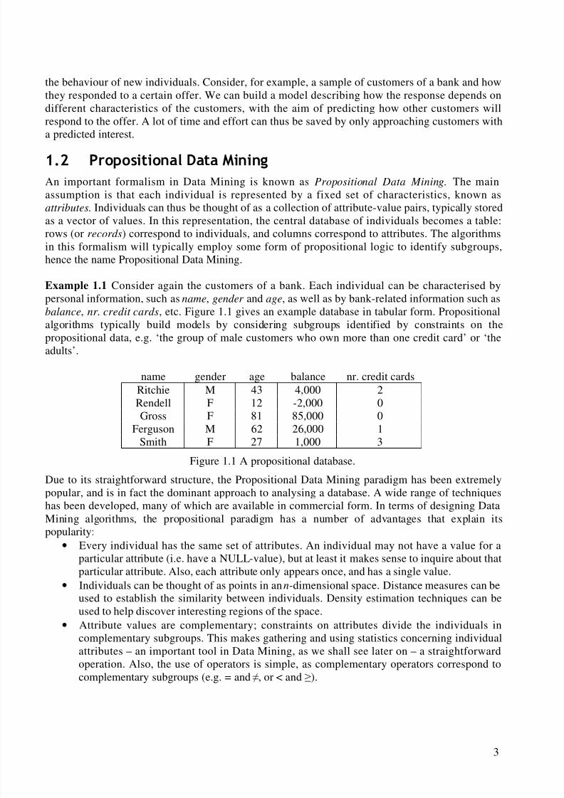
Example 1.1 Consider again the customers of a bank. Each individual can be characterised bypersonal information, such as name, gender and age, as well as by bank-related information such asbalance, nr. credit cards, etc. Figure 1.1 gives an example database in tabular form. Propositionalalgorithms typically build models by considering subgroups identified by constraints on thepropositional data, e.g. ‘the group of male customers who own more than one credit card’ or ‘theadults’.
name gender age balance nr. credit cardsRitchie M 43 4,000 2Rendell F 12 -2,000 0
Gross F 81 85,000 0Ferguson M 62 26,000 1Smith F 27 1,000 3
Figure 1.1 A propositional database.
Due to its straightforward structure, the Propositional Data Mining paradigm has been extremelypopular, and is in fact the dominant approach to analysing a database. A wide range of techniqueshas been developed, many of which are available in commercial form. In terms of designing DataMining algorithms, the propositional paradigm has a number of advantages that explain itspopularity:
• Every individual has the same set of attributes. An individual may not have a value for a
particular attribute (i.e. have a NULL-value), but at least it makes sense to inquire about thatparticular attribute. Also, each attribute only appears once, and has a single value.• Individuals can be thought of as points in an n-dimensional space. Distance measures can be
used to establish the similarity between individuals. Density estimation techniques can beused to help discover interesting regions of the space.
• Attribute values are complementary; constraints on attributes divide the individuals incomplementary subgroups. This makes gathering and using statistics concerning individualattributes – an important tool in Data Mining, as we shall see later on – a straightforwardoperation. Also, the use of operators is simple, as complementary operators correspond tocomplementary subgroups (e.g. = and , or < and ).
8/8/2019 Knobbe a.J. Multi-Relational Data Mining
http://slidepdf.com/reader/full/knobbe-aj-multi-relational-data-mining 15/129
4
• The meta-data describing the database is simple. This meta-data is used to guide the searchfor interesting subgroups, which in Propositional Data Mining boils down to addingpropositional expressions on the basis of available attributes.
There is a single, yet essential disadvantage to the propositional paradigm: there are fundamental
limitations to the expressive power of the propositional framework. Objects in the real world oftenexhibit some internal structure that is hard to fit in a tabular template. Some typical situations wherethe representational power of Propositional Data Mining is insufficient are the following:
• Real world objects often consist of parts, differing in size and number from one object to thenext. A fixed set of attributes cannot represent this variation in structure.
• Real-world objects contain parts that do not differ in size and number, but that are unorderedor interchangeable. It is impossible to assign properties of parts to particular attributes of theindividual without introducing some artificial and harmful ordering.
• Real-world objects can exhibit a recursive structure.
6WUXFWXUHG'DWD0LQLQJ
The Propositional Data Mining paradigm has been popular because of the simple tabular structure itproposes. This property is, at the same time, its weakness. Many databases, especially of largeindustrial nature, are simply too complex to analyse with a propositional algorithm without ignoringimportant information. Rather than working with individuals that can be thought of as vectors of attribute-value data, we will have to deal with structured objects that consist of parts that may beconnected in a variety of ways. Data Mining algorithms will have to consider not only attribute-value information concerning parts (which may be absent), but also important informationconcerning the presence of different types of parts, and how they are connected.
active inactive
NH2
NHN
NH2
NHN
CH3
Histamine
NH
NHN
CH3
NH2
ON
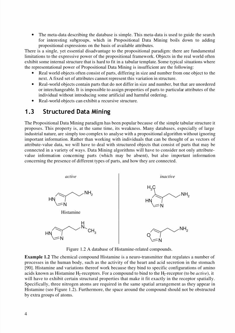
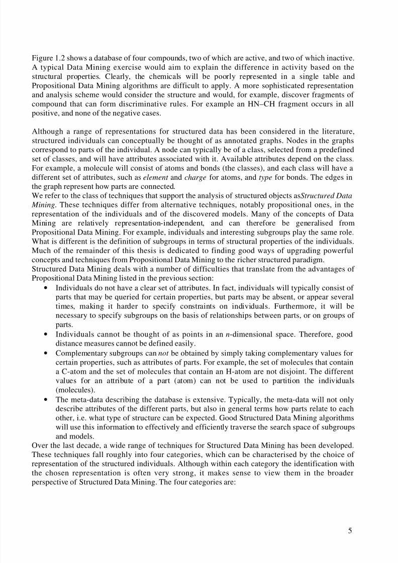
Figure 1.2 A database of Histamine-related compounds.
Example 1.2 The chemical compound Histamine is a neuro-transmitter that regulates a number of processes in the human body, such as the activity of the heart and acid secretion in the stomach[90]. Histamine and variations thereof work because they bind to specific configurations of aminoacids known as Histamine H2-receptors. For a compound to bind to the H2-receptor (to be active), itwill have to exhibit certain structural properties that make it fit exactly in the receptor spatially.Specifically, three nitrogen atoms are required in the same spatial arrangement as they appear in
Histamine (see Figure 1.2). Furthermore, the space around the compound should not be obstructedby extra groups of atoms.
8/8/2019 Knobbe a.J. Multi-Relational Data Mining
http://slidepdf.com/reader/full/knobbe-aj-multi-relational-data-mining 16/129
5
Figure 1.2 shows a database of four compounds, two of which are active, and two of which inactive.A typical Data Mining exercise would aim to explain the difference in activity based on thestructural properties. Clearly, the chemicals will be poorly represented in a single table andPropositional Data Mining algorithms are difficult to apply. A more sophisticated representation
and analysis scheme would consider the structure and would, for example, discover fragments of compound that can form discriminative rules. For example an HN–CH fragment occurs in allpositive, and none of the negative cases.
Although a range of representations for structured data has been considered in the literature,structured individuals can conceptually be thought of as annotated graphs. Nodes in the graphscorrespond to parts of the individual. A node can typically be of a class, selected from a predefinedset of classes, and will have attributes associated with it. Available attributes depend on the class.For example, a molecule will consist of atoms and bonds (the classes), and each class will have adifferent set of attributes, such as element and charge for atoms, and type for bonds. The edges inthe graph represent how parts are connected.
We refer to the class of techniques that support the analysis of structured objects as Structured Data Mining. These techniques differ from alternative techniques, notably propositional ones, in therepresentation of the individuals and of the discovered models. Many of the concepts of DataMining are relatively representation-independent, and can therefore be generalised fromPropositional Data Mining. For example, individuals and interesting subgroups play the same role.What is different is the definition of subgroups in terms of structural properties of the individuals.Much of the remainder of this thesis is dedicated to finding good ways of upgrading powerfulconcepts and techniques from Propositional Data Mining to the richer structured paradigm.Structured Data Mining deals with a number of difficulties that translate from the advantages of Propositional Data Mining listed in the previous section:
• Individuals do not have a clear set of attributes. In fact, individuals will typically consist of
parts that may be queried for certain properties, but parts may be absent, or appear severaltimes, making it harder to specify constraints on individuals. Furthermore, it will benecessary to specify subgroups on the basis of relationships between parts, or on groups of parts.
• Individuals cannot be thought of as points in an n-dimensional space. Therefore, gooddistance measures cannot be defined easily.
• Complementary subgroups can not be obtained by simply taking complementary values forcertain properties, such as attributes of parts. For example, the set of molecules that containa C-atom and the set of molecules that contain an H-atom are not disjoint. The differentvalues for an attribute of a part (atom) can not be used to partition the individuals(molecules).
• The meta-data describing the database is extensive. Typically, the meta-data will not onlydescribe attributes of the different parts, but also in general terms how parts relate to eachother, i.e. what type of structure can be expected. Good Structured Data Mining algorithmswill use this information to effectively and efficiently traverse the search space of subgroupsand models.
Over the last decade, a wide range of techniques for Structured Data Mining has been developed.These techniques fall roughly into four categories, which can be characterised by the choice of representation of the structured individuals. Although within each category the identification withthe chosen representation is often very strong, it makes sense to view them in the broaderperspective of Structured Data Mining. The four categories are:
8/8/2019 Knobbe a.J. Multi-Relational Data Mining
http://slidepdf.com/reader/full/knobbe-aj-multi-relational-data-mining 17/129
6
• Graph Mining [19, 48, 79, 80] The database consists of labelled graphs, and graphmatching is used to select individuals on the basis of substructures that may or may not bepresent.
• Inductive Logic Programming (ILP) [9, 11, 12, 13, 14, 22, 28, 30, 31, 70, 83, 89] The
database consists of a collection of facts in first-order logic. Each fact represents a part, andindividuals can be reconstructed by piecing together these facts. First-order logic (oftenProlog) can be used to select subgroups.
• Semi-Structured Data Mining [1, 8, 16, 81, 104] The database consists of XML-documents, which describe objects in a mixture of structural and free-text information.
• Multi-Relational Data Mining (MRDM) [7, 31, 53, 59, 61, 62, 63, 74, 107] The databaseconsists of a collection of tables (a relational database). Records in each table representparts, and individuals can be reconstructed by joining over the foreign key relations betweenthe tables. Subgroups can be defined by means of SQL or a graphical query languagepresented in Chapter 4.
In Chapter 2 we will examine Structured Data Mining in depth, and compare the four categories of
techniques according to how they approach different aspects of structured data.
0XOWL5HODWLRQDO'DWD0LQLQJ
The approach to Structured Data Mining that is the main subject of this thesis, Multi-RelationalData Mining, is inspired by the relational model [21, 100, 101]. This model presents a number of techniques to store, manipulate and retrieve complex and structured data in a database consisting of a collection of tables. It has been the dominant paradigm for industrial database applications duringthe last decades, and it is at the core of all major commercial database systems, commonly knownas relational database management systems (RDBMS). A relational database consists of a collectionof named tables, often referred to as relations that individually behave as the single table that is the
subject of Propositional Data Mining. Data structures more complex than a single record areimplemented by relating pairs of tables through so-called foreign key relations. Such a relationspecifies how certain columns in one table can be used to look up information in correspondingcolumns in the other table, thus relating sets of records in the two tables.Structured individuals (graphs) are represented in a relational database in a distributed fashion. Eachpart of the individual (node) appears as a single record in one of the tables. All parts of the sameclass for all individuals appear in the same table. By following the foreign keys (edges), differentparts can be joined in order to reconstruct an individual. In our search for patterns in the relationaldatabase, we will need to query individuals for certain structural properties. Relational databasetheory employs two popular languages for retrieving information from a relational database:relational algebra and the Structured Query Language (SQL). The former is primarily used in the
theoretical settings, whereas the latter is primarily used in practical systems. SQL is supported byall major RDBMSs. In this thesis we employ an additional (graphical) language that selectsindividuals on the basis of structural properties of the graphs. This language translates easily intoSQL, but is preferable because manipulation of structural expressions is more intuitive.
2XWOLQHRIWKLVWH[W
This thesis is structured as follows. The following three chapters contain an introductory text,detailing the concepts and techniques relevant for Structured Data Mining in general and Multi-Relational Data Mining in specific. Chapter 2 defines major concepts shared by all SDM paradigms,and demonstrates how each paradigm implements these concepts. Chapters 3 and 4 define in more
detail how our MRDM approach works. It covers how structured individuals are represented and
8/8/2019 Knobbe a.J. Multi-Relational Data Mining
http://slidepdf.com/reader/full/knobbe-aj-multi-relational-data-mining 18/129
7
queried in a relational database. Parts of these chapters were previously published in the followingpapers:
Knobbe, A., Siebes, A., Blockeel, H., Van der Wallen, D. Multi-Relational Data Mining,
using UML for ILP, In Proceedings of PKDD 2000, LNAI 1910, 2000Knobbe, A., Blockeel, H., Siebes, A., Van der Wallen, D. Multi-Relational Data Mining, InProceedings of Benelearn ’99, 1999
Chapter 5, Multi-Relational Rule Discovery and Chapter 6, Multi-Relational Decision TreeInduction, cover two important mining techniques in MRDM. Both techniques are based on aparticular means of capturing structural features. The text in these chapters is based on the secondpaper mentioned above, as well as the following paper:
Knobbe, A., Siebes, A., Van der Wallen, D. Multi-Relational Decision Tree Induction, In
Proceedings of PKDD ’99, LNAI 1704, pp. 378-383, 1999
Chapters 7 through 9 investigate an alternative way of extracting structural features, namely bymeans of aggregate functions. Chapter 7, Aggregate Functions, provides the necessary preliminariesfor the subsequent chapters. In Chapter 8, Aggregate Functions & Propositionalisation, we present amethod to flatten a multi-relational database using these aggregate functions in order to analyse theresulting table using traditional techniques. This method was previously published in the followingpaper:
Knobbe, A., De Haas, M., Siebes, A. Propositionalisation and Aggregates, In Proceedingsof PKDD 2001, LNAI 2168, pp. 277-288, 2001
Chapter 9 describes how this richer method of capturing structured features can be integrated in therule discovery techniques introduced in Chapter 5. This method was previously published in:
Knobbe, A., Siebes, A., Marseille, B. Involving Aggregate Functions in Multi-Relational
Search, In Proceedings of PKDD 2002, LNAI 2431, 2002
Chapter 10, MRDM Primitives, covers how MRDM techniques can gather the necessary statisticsfrom the database using a predefined set of queries. This subject has appeared in most of the above-mentioned papers.
Chapter 11 considers MRDM on a more methodological level. It provides a blueprint for MRDMprojects, focussing on the activities that precede the actual modelling step, and presents ProSafarii,a system that supports a user in the pre-processing phase of MRDM projects.
Finally, Chapter 12 concludes with a discussion and pointers for future work.

8/8/2019 Knobbe a.J. Multi-Relational Data Mining
http://slidepdf.com/reader/full/knobbe-aj-multi-relational-data-mining 19/129
This page intentionally left blank
8/8/2019 Knobbe a.J. Multi-Relational Data Mining
http://slidepdf.com/reader/full/knobbe-aj-multi-relational-data-mining 20/129
9
6WUXFWXUHG'DWD0LQLQJ
In this chapter we give an overview of the genus of Data Mining paradigms that deal withstructured data. We start with definitions of the major concepts in Structured Data Mining having todo with how structured data is represented and how knowledge can be extracted from this data.These concepts are shared by the different SDM paradigms that are the subject of the remainingsections of this chapter. We briefly outline each approach, and describe how they implement SDM.Subsequently, we describe on a more detailed level the strengths and weaknesses of each paradigm.
6WUXFWXUHG'DWD
As was outlined in Chapter 1, the central subject of analysis is the individual. We assume inStructured Data Mining that an individual consist of parts that are somehow connected to form astructured individual. Parts can be thought of as small portions of an individual that are atomic: theyexhibit no internal structure. All structural relations are between parts, rather than within parts. Partstypically have a number of attributes associated with them. They can thus be thought of as tuplesthat behave similar to the flat individuals that are the subject of Propositional Data Mining. Ingeneral, structured individuals will not be arbitrary collections of parts. Parts will appear in arelatively small number of types, referred to as classes. All parts, over all individuals, are instancesof one of the classes. A class determines which attributes are available for all instances of that class.
Definition 2.1 A class C is a triple (c, S, D) in which c is the class-name, S is the schema, a set of
attributes with their domain S = {a1 : D1, …, an : Dn}, and D is the domain of C : DC = ∏=
n
i
i D1
.
Definition 2.2 A part of class C is a tuple (a1, …, an) ∈ DC .
Not just the characteristics of parts are important in Structured Data Mining, but also how theyrelate to form structured individuals. We will think of individuals as annotated graphs, where thenodes represent the parts. Labelled, but undirected, edges between parts represent the relationshipbetween pairs of parts. Other than the label, the edge provides no information concerning therelationship between the parts. Typically, there will not be edges between arbitrary pairs of parts.Most data representation schemes will only allow relations between specific classes of parts to
enforce certain types of structure in the individuals. Furthermore, there will often be restrictions on
8/8/2019 Knobbe a.J. Multi-Relational Data Mining
http://slidepdf.com/reader/full/knobbe-aj-multi-relational-data-mining 21/129
10
the number of parts of a certain class that may be related to a part of some other class, and viceversa. A definition of the restrictions on relations between parts of two classes will be referred to asan association between two classes. Edges in an individual can thus be thought of as instances of anassociation, where the label refers to the association. It should be noted that this use of the term
association is not related to the term association rules, which indicates a popular family of modelsof statistical dependency [33]. The present associations are hard constraints on the data.The central input to the Structured Data Mining process is now the database, simply a collection of individuals. Although each individual will most probably be different in parts and structure, the setof individuals will adhere to a common set of restrictions on the appearance of individuals. Thiscollection of restrictions is referred to as the data model of the database, and consists of thedefinitions of available classes (including attributes) of parts, plus the definitions of associationsbetween classes.
Example 2.1 Consider a database of molecule-descriptions. Each individual describes a molecule,and consists of parts that come in three classes: a piece of information describing general properties
of the molecule (molecule), pieces of information for each atom (atom), and pieces of informationfor each bond between two atoms (bond). Each of these classes has a fixed set of attributes, forexample atom has attributes element and charge. The parts of these three classes are related to eachother through four associations: one determines which atoms belong to which molecule. Similarlythere is an association that determines which bond belongs to which molecule. The two remainingassociations determine the two atoms involved in each bond.
Definition 2.3 A data model is a rooted undirected connected graph M = (C , A), where:1. C is a set of class-names2. A ⊆ C × C such that, if (c, d ) ∈ A, then (d, c) ∈ A.
The elements of A are called associations. The root of the graph is denoted by c0.
Definition 2.4 An individual for data model M = (C, A) is a rooted undirected connected graph i =(P, E ), where P is a set of parts, and E is a set of triples ( p, q, a) such that
1. a = (c, d ) ∈ A
2. p is a part of class c, and q is a part of class d
3. there is a unique part p0 ∈ P such that if ( p, q, (c0, ci)) ∈ E , then p = p0.The set of all individuals for a data model M is denoted by L M .
Definition 2.5 A database for data model M is a set of individuals for M .
6HDUFK
In Chapter 1 we briefly mentioned the interesting subgroup as an important ingredient of DataMining algorithms. A large number of subgroups will be considered by such algorithms in order toproduce a manageable set of interesting subgroups that will be the basis for higher-level models of the database. Rather than being interested in subgroups as enumerations of individuals belonging toit (extensional approach), we consider short descriptions of the properties shared by all members of the subgroup (intensional approach). We refer to such descriptions as patterns. In Structured DataMining, patterns express certain required properties concerning the presence of certain parts andstructural relationships between them. Patterns can thus be used to match individuals, and definesubgroups.In order to express and manipulate patterns, we require a pattern language. As the individuals are
structured, the pattern language will need to be able to express structural properties. Because of our
8/8/2019 Knobbe a.J. Multi-Relational Data Mining
http://slidepdf.com/reader/full/knobbe-aj-multi-relational-data-mining 22/129
11
definition of individuals as graphs, the language will conceptually be graphical. In fact, a number of Structured Data Mining paradigms, including the Multi-Relational Data Mining approach wepresent in this thesis, use variations of graphs as patterns. Other paradigms, Inductive LogicProgramming and Semi-Structured Data Mining, rely on existing languages for expressing
structural constraints.Definition 2.6 A pattern language is a pair L p = (P, covers) such that P is a set of expressions, andcovers is a function P × L M → {0, 1}. A pattern p ∈ P is said to cover an individual i ∈ L M iff
covers( p, i) = 1. If clear from the context, we will often write L p to denote P.
Definition 2.7 A pattern in a pattern language L p = (P, C ) is an expression p ∈ P.
Definition 2.8 A subgroup S p is a set of individuals in a database D that is covered by a givenpattern p: S p = {i ∈ D | covers( p, i)}.
Example 2.2 Consider a database D of individuals i = ( N , E ), and the pattern language L p = (P,covers), where P is the set of graphs G = ( N ′, E ′), and covers(G, i) iff there exists an injection M : N ′→ N, such that
∀e ∈ E ′: ( M (e.p), M (e.q), a) ∈ E
where a is an uninstantiated variable representing an unspecified association. This pattern languagecan be used to describe particular subgraphs that may or may not appear in individuals in D. Thelocation of the root of the individuals, as well as the class and attributes of its parts are ignored. Byrefining P and adding more constraints on the injection M , we can define more expressive patternlanguages.
Most Data Mining algorithms are characterised by an extensive search for interesting subgroups.The pattern language of choice defines a search space of patterns, which is the starting point for thissearch process. In order to traverse this space in a sensible, guided and efficient manner, thealgorithm requires a means of judging the interestingness of a given pattern (and correspondingsubgroup). In general terms we refer to such a means as a score function. Typically a score functionconsiders the database and acquires statistics about the pattern at hand, which in turn produces ascore. This score will help the algorithm to make informed decisions about the progress anddirection of the search.Most algorithms will not only use statistical information from the database to guide the search, butalso a priori information about the kind of individuals that are known to exist in the database. Theconstraints contained in the data model concerning classes and associations tell us that we cannotexpect arbitrary structures in the database. Rather, we can limit the search to patterns that are incorrespondence with the data model. Restrictions on the search space based on a priori knowledgeabout the database, commonly referred to as declarative bias, are a very important means of keeping the search process manageable and efficient. We will consider different ways of exploitingdeclarative bias in Multi-Relational Data Mining throughout this thesis.
Definition 2.9 A score function is function f : L p × M L2 R such that, given a database D and twopatterns p and q, S p = Sq f ( p, D) = f (q, D).
Definition 2.10 A declarative bias is a set of constraints on the patterns considered by a DataMining algorithm.
8/8/2019 Knobbe a.J. Multi-Relational Data Mining
http://slidepdf.com/reader/full/knobbe-aj-multi-relational-data-mining 23/129
12
Because we know that the search is strongly guided by the data model of the database, we canexpect a certain similarity and order in the candidate patterns to be considered. Typically, a patternwill be tested on the database by means of the score function(s), and new candidate patterns will bederived from the pattern with the obtained statistics in mind. The important step of deriving new
patterns by means of minimal additions to an existing pattern is known as refinement . We will beusing a refinement operator , which specifies what syntactic operations are allowed on a givenpattern in order to derive more complex patterns.The predominant search mode in Data Mining is top-down search: start with a very general pattern,and progressively consider more specific patterns. For this, we require the refinement operator toproduce subgroups that are subsets of the original subgroup. We refer to a refinement operator withthis additional property as a top-down refinement operator.
Definition 2.11 A pattern p is more general than a pattern q ( p ≥ q) if all individuals covered by q
are also covered by p:( p ≥ q) iff ∀i : covers(q, i) covers( p, i).
Definition 2.12 A specialisation operator is a function : L p 2 Lp such that ∀ p ∈ L p: ( p) ⊆ {q | p
≥ q}.
Definition 2.13 A refinement operator is a function : L p 2 Lp such that, given a set of syntacticoperations, ∀ p ∈ L p : ( p) = {q | q is the result of a syntactic operation on p}.
Definition 2.14 A top-down refinement operator is a refinement operator that is also aspecialisation operator.
6WUXFWXUHG'DWD0LQLQJ3DUDGLJPVThe basic definitions given in the previous section outline how Structured Data Mining works ingeneral terms. The existing Structured Data Mining paradigms as introduced in Chapter 1 all exhibitthese concepts in one form or another, but we will need to consider how each paradigm implementsthem. This will help us translate terminology and practices from one paradigm to the other.Furthermore, by viewing paradigms as instances of a generic Data Mining approach, we will beable to distinguish the properties shared by all paradigms from those that are unique to a particularparadigm. We will start with an overview of the commonalities by considering how the differentparadigms implement Structured Data Mining concepts.
Graph Mining From all four Data Mining paradigms for dealing with structured data, the GraphMining paradigm is closest in approach to our abstract definition of structured Data Mining.Individuals are simply (labelled) graphs, and the database is hence a forest of these graphs. In mostapproaches a node (part) is labelled, such that each part belongs to a class. Constraints on thestructure of individuals in the form of a data model are typically not present. The same graphicallanguage used to represent individuals is used as a pattern language. Graph matching is used todetermine which individuals are covered by a particular pattern.
Inductive Logic Programming (ILP) The ILP paradigm employs (small) logic programs todescribe patterns. The logic programs need to be induced from a database of logical facts, hence thename Inductive Logic Programming. The facts in the database represent parts of the structured
individual. The class of each part can be identified by the predicate of the fact. The notion of individual is rarely made explicit, although sometimes facts are grouped together, or keys are added
8/8/2019 Knobbe a.J. Multi-Relational Data Mining
http://slidepdf.com/reader/full/knobbe-aj-multi-relational-data-mining 24/129
13
to identify the individual. A variety of declarative bias languages is used, but they mostly share theuse of mode declarations [31] in order to describe how parts can be pieced together. Modedeclarations restrict how certain attributes in certain predicates may be linked by shared variables inthe induced logic programs. This is a slight variation on the association concept. ILP typically uses
Prolog as the pattern language. ILP algorithms often allow as input not only the database of groundfacts, but also intensional predicate definitions that may help the search process for interestingpatterns.
Semi-Structured Data Mining (SSDM) The most recent approach to mining in structured data,Semi-Structured Data Mining deals with a database of semi-structured text, typically represented inthe popular language XML [2, 17, 32]. Although semi-structured documents contain both structuralinformation as well as fragments of free text, most approaches focus on the structural part and treatthe text fragments as discrete values without internal structure. XML documents essentiallyrepresent a rooted tree, where the tree-structure is identified by markers in the text, known as tags,and free-text appears at the nodes (and leaves) of the tree.
The existing SSDM approaches treat documents in two technically different, but effectively similarways. One approach is to treat a single document as the database, and regard the children of the rootof the semi-structured tree as individuals. The alternative approach is to take a collection of documents as the database, and treat each document as an individual. In either way, the nodes in thetree, identified by tags, correspond to the parts, and may have several attributes.Most XML documents come with a grammar that strongly restricts the kinds of structure that areallowed in XML documents. Typically this grammar is specified in a separate file, known as aDocument Type Definition (DTD) [41], which may be shared by multiple documents. Althoughrarely used in SSDM, DTD is ideal as a declarative bias. In the true nature of declarative bias, aDTD not only determines when XML documents are well formed, but should be used as importantinformation to guide and prune the search process. The existing SSDM approaches boast a variety
of pattern languages in order to select individuals on the basis of features of the semi-structuredtree. Most algorithms employ generic graphical or tree structures that are not specific to thetechnology surrounding XML. A new development is to use the XPath technology [108] that hasbeen specifically designed for applications that need to access and query specific locations withinXML documents. It can be expected that XPath, or more generally XQuery [109], will play agreater role as pattern language for SSDM in the future [16].
MRDM ILP GM SSDMdatabase language relational DB Prolog graphs XML
bias language UML/ER various – DTD
pattern language SQL/SG Prolog graphs graphs/XQueryTable 2.1 Representation in Structured Data Mining approaches.
$&RPSDULVRQ
The general overview of approaches to mining structured data given in the previous sectionsuggests that the paradigms mainly differ on a syntactical level. All paradigms exhibit the basicfeatures of Structured Data Mining, albeit in a different representational framework. Table 2.1summarises these representational differences for some important concepts. At first glance, theapproaches seem interchangeable if we can simply translate between representations. However, on a
more detailed level, the choice of representation does have effects on different aspects of the dataand hence on the power of the mining paradigm. Below, we give a brief comparison of some of
8/8/2019 Knobbe a.J. Multi-Relational Data Mining
http://slidepdf.com/reader/full/knobbe-aj-multi-relational-data-mining 25/129
14
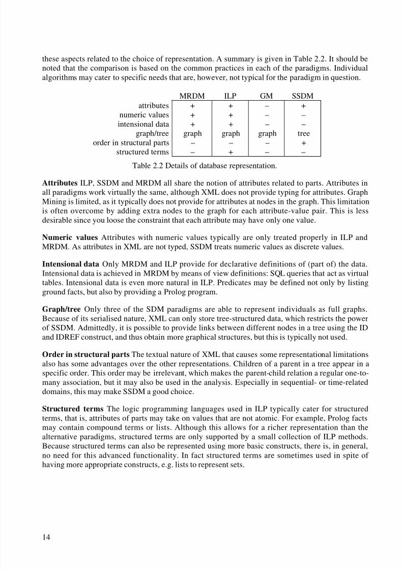
these aspects related to the choice of representation. A summary is given in Table 2.2. It should benoted that the comparison is based on the common practices in each of the paradigms. Individualalgorithms may cater to specific needs that are, however, not typical for the paradigm in question.
MRDM ILP GM SSDMattributes + + – +numeric values + + – –intensional data + + – –
graph/tree graph graph graph treeorder in structural parts – – – +
structured terms – + – –
Table 2.2 Details of database representation.
Attributes ILP, SSDM and MRDM all share the notion of attributes related to parts. Attributes inall paradigms work virtually the same, although XML does not provide typing for attributes. Graph
Mining is limited, as it typically does not provide for attributes at nodes in the graph. This limitationis often overcome by adding extra nodes to the graph for each attribute-value pair. This is lessdesirable since you loose the constraint that each attribute may have only one value.
Numeric values Attributes with numeric values typically are only treated properly in ILP andMRDM. As attributes in XML are not typed, SSDM treats numeric values as discrete values.
Intensional data Only MRDM and ILP provide for declarative definitions of (part of) the data.Intensional data is achieved in MRDM by means of view definitions: SQL queries that act as virtualtables. Intensional data is even more natural in ILP. Predicates may be defined not only by listingground facts, but also by providing a Prolog program.
Graph/tree Only three of the SDM paradigms are able to represent individuals as full graphs.Because of its serialised nature, XML can only store tree-structured data, which restricts the powerof SSDM. Admittedly, it is possible to provide links between different nodes in a tree using the IDand IDREF construct, and thus obtain more graphical structures, but this is typically not used.
Order in structural parts The textual nature of XML that causes some representational limitationsalso has some advantages over the other representations. Children of a parent in a tree appear in aspecific order. This order may be irrelevant, which makes the parent-child relation a regular one-to-many association, but it may also be used in the analysis. Especially in sequential- or time-relateddomains, this may make SSDM a good choice.
Structured terms The logic programming languages used in ILP typically cater for structuredterms, that is, attributes of parts may take on values that are not atomic. For example, Prolog factsmay contain compound terms or lists. Although this allows for a richer representation than thealternative paradigms, structured terms are only supported by a small collection of ILP methods.Because structured terms can also be represented using more basic constructs, there is, in general,no need for this advanced functionality. In fact structured terms are sometimes used in spite of having more appropriate constructs, e.g. lists to represent sets.
8/8/2019 Knobbe a.J. Multi-Relational Data Mining
http://slidepdf.com/reader/full/knobbe-aj-multi-relational-data-mining 26/129
15
MRDM ILP GM SSDMrecursion – + – –
aggregate functions + – – –numeric data + – – –
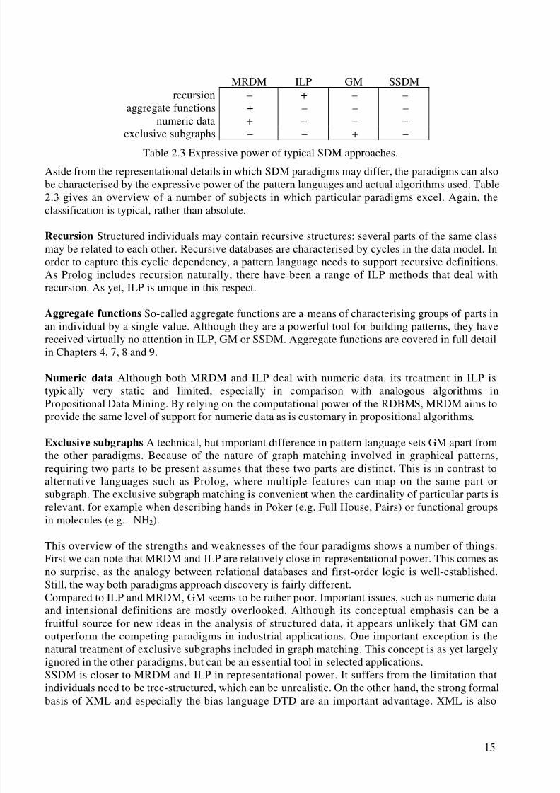
exclusive subgraphs – – + –Table 2.3 Expressive power of typical SDM approaches.
Aside from the representational details in which SDM paradigms may differ, the paradigms can alsobe characterised by the expressive power of the pattern languages and actual algorithms used. Table2.3 gives an overview of a number of subjects in which particular paradigms excel. Again, theclassification is typical, rather than absolute.
Recursion Structured individuals may contain recursive structures: several parts of the same classmay be related to each other. Recursive databases are characterised by cycles in the data model. Inorder to capture this cyclic dependency, a pattern language needs to support recursive definitions.
As Prolog includes recursion naturally, there have been a range of ILP methods that deal withrecursion. As yet, ILP is unique in this respect.
Aggregate functions So-called aggregate functions are a means of characterising groups of parts inan individual by a single value. Although they are a powerful tool for building patterns, they havereceived virtually no attention in ILP, GM or SSDM. Aggregate functions are covered in full detailin Chapters 4, 7, 8 and 9.
Numeric data Although both MRDM and ILP deal with numeric data, its treatment in ILP istypically very static and limited, especially in comparison with analogous algorithms inPropositional Data Mining. By relying on the computational power of the RDBMS, MRDM aims to
provide the same level of support for numeric data as is customary in propositional algorithms.
Exclusive subgraphs A technical, but important difference in pattern language sets GM apart fromthe other paradigms. Because of the nature of graph matching involved in graphical patterns,requiring two parts to be present assumes that these two parts are distinct. This is in contrast toalternative languages such as Prolog, where multiple features can map on the same part orsubgraph. The exclusive subgraph matching is convenient when the cardinality of particular parts isrelevant, for example when describing hands in Poker (e.g. Full House, Pairs) or functional groupsin molecules (e.g. –NH2).
This overview of the strengths and weaknesses of the four paradigms shows a number of things.
First we can note that MRDM and ILP are relatively close in representational power. This comes asno surprise, as the analogy between relational databases and first-order logic is well-established.Still, the way both paradigms approach discovery is fairly different.Compared to ILP and MRDM, GM seems to be rather poor. Important issues, such as numeric dataand intensional definitions are mostly overlooked. Although its conceptual emphasis can be afruitful source for new ideas in the analysis of structured data, it appears unlikely that GM canoutperform the competing paradigms in industrial applications. One important exception is thenatural treatment of exclusive subgraphs included in graph matching. This concept is as yet largelyignored in the other paradigms, but can be an essential tool in selected applications.SSDM is closer to MRDM and ILP in representational power. It suffers from the limitation thatindividuals need to be tree-structured, which can be unrealistic. On the other hand, the strong formalbasis of XML and especially the bias language DTD are an important advantage. XML is also
8/8/2019 Knobbe a.J. Multi-Relational Data Mining
http://slidepdf.com/reader/full/knobbe-aj-multi-relational-data-mining 27/129
8/8/2019 Knobbe a.J. Multi-Relational Data Mining
http://slidepdf.com/reader/full/knobbe-aj-multi-relational-data-mining 28/129
17
0XOWL5HODWLRQDO'DWD
In the previous chapter, a general framework for mining structured data was outlined, and anoverview was given of how the different Structured Data Mining paradigms approach such data. Inthis and the following chapter, we will describe in more detail how MRDM works, and introducesome basic concepts upon which the different MRDM techniques described in following chapterswill build. We will explain how structured data is stored in a relational database, and how MRDMalgorithms may query such data. A multi-relational pattern language will be introduced, along witha refinement operator that lays out a search space of multi-relational patterns for MRDM algorithmsto explore.
6WUXFWXUHG'DWDLQ5HODWLRQDO)RUP
Structured data will always be represented in a relational database by multiple tables. Theinformation concerning the different parts of an individual will be distributed over these tables.There is one particular table, which we will refer to as the target table, that has a special role. Each
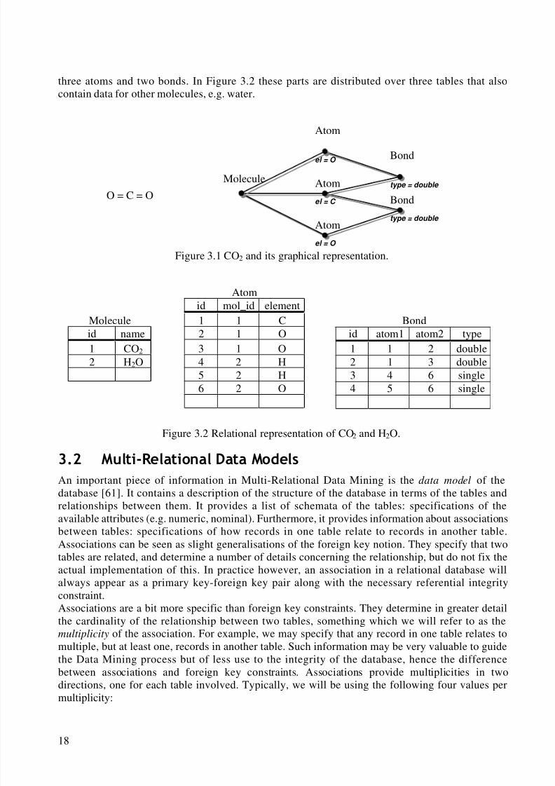
record in this table corresponds to exactly one individual. The target table will be connected to othertables through foreign key relations. By following these keys the remaining data concerningindividuals may be looked up. The target table will always be the starting point for searchinginteresting patterns, as patterns represent sets of individuals. The target table will often containattributes that describe individuals as a whole, but may also just contain a single key-attribute thatpoints to the structural parts in the remaining tables. Each table contains parts belonging to oneparticular class. All parts of this class, regardless of the individual, appear in the same table. Inorder to determine the individual that a part belongs to, or to collect all parts belonging to a givenindividual, one will have to join over the foreign key relations. Figure 3.1 and Figure 3.2 give anexample of how molecules may be stored in a relational database for multi-relational analysis.Figure 3.1 demonstrates how carbon dioxide consists of six parts in three classes: one molecule,
8/8/2019 Knobbe a.J. Multi-Relational Data Mining
http://slidepdf.com/reader/full/knobbe-aj-multi-relational-data-mining 29/129
18
three atoms and two bonds. In Figure 3.2 these parts are distributed over three tables that alsocontain data for other molecules, e.g. water.
Figure 3.1 CO2 and its graphical representation.
Atomid mol_id element
Molecule 1 1 C Bondid name 2 1 O id atom1 atom2 type1 CO2 3 1 O 1 1 2 double2 H2O 4 2 H 2 1 3 double
5 2 H 3 4 6 single6 2 O 4 5 6 single
Figure 3.2 Relational representation of CO2 and H2O.
0XOWL5HODWLRQDO'DWD0RGHOV
An important piece of information in Multi-Relational Data Mining is the data model of thedatabase [61]. It contains a description of the structure of the database in terms of the tables andrelationships between them. It provides a list of schemata of the tables: specifications of theavailable attributes (e.g. numeric, nominal). Furthermore, it provides information about associationsbetween tables: specifications of how records in one table relate to records in another table.Associations can be seen as slight generalisations of the foreign key notion. They specify that twotables are related, and determine a number of details concerning the relationship, but do not fix theactual implementation of this. In practice however, an association in a relational database willalways appear as a primary key-foreign key pair along with the necessary referential integrityconstraint.Associations are a bit more specific than foreign key constraints. They determine in greater detailthe cardinality of the relationship between two tables, something which we will refer to as themultiplicity of the association. For example, we may specify that any record in one table relates tomultiple, but at least one, records in another table. Such information may be very valuable to guidethe Data Mining process but of less use to the integrity of the database, hence the differencebetween associations and foreign key constraints. Associations provide multiplicities in two
directions, one for each table involved. Typically, we will be using the following four values permultiplicity:
Atom
Atom
Atom
Molecule
Bond
Bondel = C
el = O
type = double
type = double
O = C = O
el = O
8/8/2019 Knobbe a.J. Multi-Relational Data Mining
http://slidepdf.com/reader/full/knobbe-aj-multi-relational-data-mining 30/129
19
• Zero or one (0..1)• One (1)• Zero or more (0..n)• One or more (1..n)
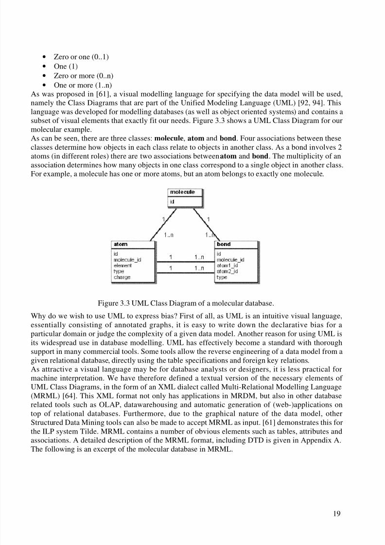
As was proposed in [61], a visual modelling language for specifying the data model will be used,namely the Class Diagrams that are part of the Unified Modeling Language (UML) [92, 94]. Thislanguage was developed for modelling databases (as well as object oriented systems) and contains asubset of visual elements that exactly fit our needs. Figure 3.3 shows a UML Class Diagram for ourmolecular example.As can be seen, there are three classes: molecule, atom and bond. Four associations between theseclasses determine how objects in each class relate to objects in another class. As a bond involves 2atoms (in different roles) there are two associations between atom and bond. The multiplicity of anassociation determines how many objects in one class correspond to a single object in another class.For example, a molecule has one or more atoms, but an atom belongs to exactly one molecule.
Figure 3.3 UML Class Diagram of a molecular database.
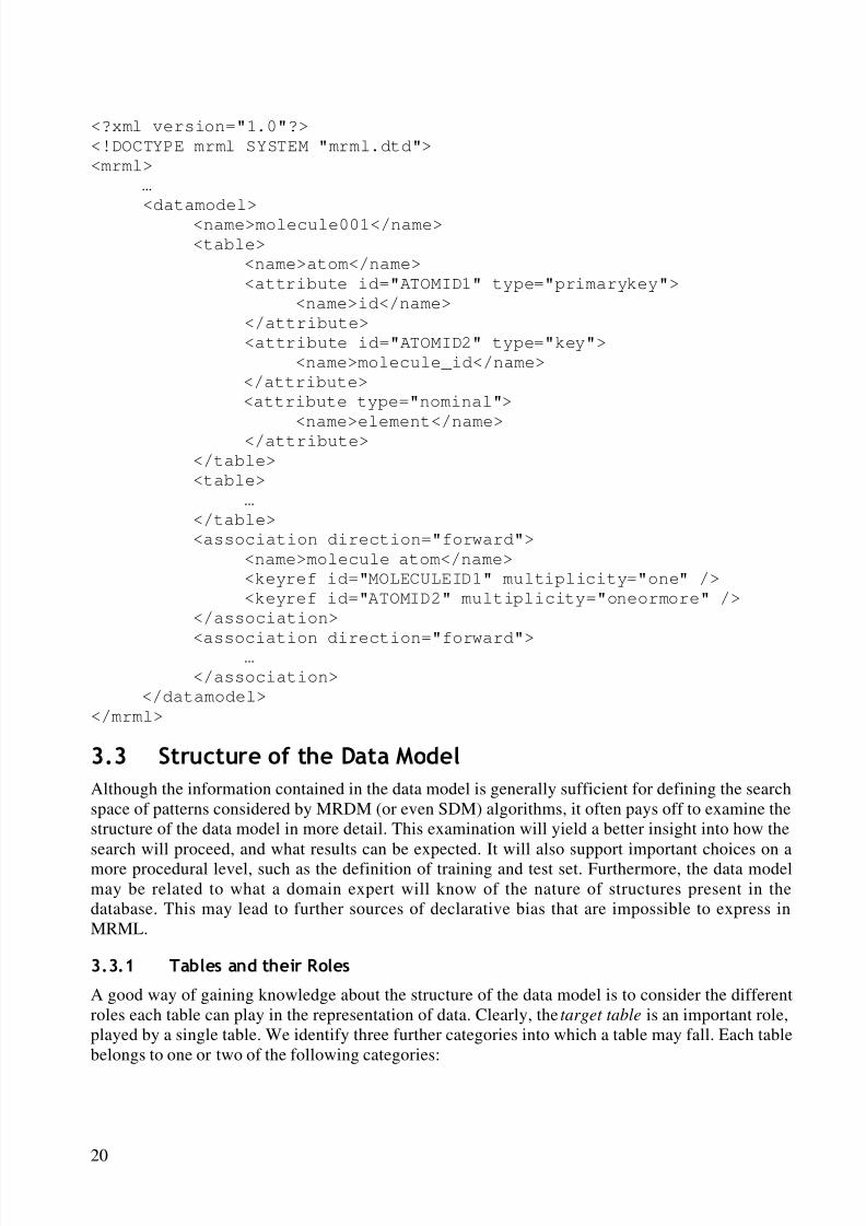
Why do we wish to use UML to express bias? First of all, as UML is an intuitive visual language,essentially consisting of annotated graphs, it is easy to write down the declarative bias for aparticular domain or judge the complexity of a given data model. Another reason for using UML isits widespread use in database modelling. UML has effectively become a standard with thoroughsupport in many commercial tools. Some tools allow the reverse engineering of a data model from agiven relational database, directly using the table specifications and foreign key relations.As attractive a visual language may be for database analysts or designers, it is less practical for
machine interpretation. We have therefore defined a textual version of the necessary elements of UML Class Diagrams, in the form of an XML dialect called Multi-Relational Modelling Language(MRML) [64]. This XML format not only has applications in MRDM, but also in other databaserelated tools such as OLAP, datawarehousing and automatic generation of (web-)applications ontop of relational databases. Furthermore, due to the graphical nature of the data model, otherStructured Data Mining tools can also be made to accept MRML as input. [61] demonstrates this forthe ILP system Tilde. MRML contains a number of obvious elements such as tables, attributes andassociations. A detailed description of the MRML format, including DTD is given in Appendix A.The following is an excerpt of the molecular database in MRML.
8/8/2019 Knobbe a.J. Multi-Relational Data Mining
http://slidepdf.com/reader/full/knobbe-aj-multi-relational-data-mining 31/129
20
<?xml version="1.0"?>
<!DOCTYPE mrml SYSTEM "mrml.dtd">
<mrml>
…
<datamodel>
<name>molecule001</name>
<table>
<name>atom</name>
<attribute id="ATOMID1" type="primarykey">
<name>id</name>
</attribute>
<attribute id="ATOMID2" type="key">
<name>molecule_id</name>
</attribute>
<attribute type="nominal">
<name>element</name>
</attribute>
</table>
<table>
…
</table>
<association direction="forward">
<name>molecule atom</name>
<keyref id="MOLECULEID1" multiplicity="one" />
<keyref id="ATOMID2" multiplicity="oneormore" />
</association>
<association direction="forward">…
</association>
</datamodel>
</mrml>
6WUXFWXUHRIWKH'DWD0RGHO
Although the information contained in the data model is generally sufficient for defining the searchspace of patterns considered by MRDM (or even SDM) algorithms, it often pays off to examine thestructure of the data model in more detail. This examination will yield a better insight into how thesearch will proceed, and what results can be expected. It will also support important choices on amore procedural level, such as the definition of training and test set. Furthermore, the data modelmay be related to what a domain expert will know of the nature of structures present in thedatabase. This may lead to further sources of declarative bias that are impossible to express inMRML.
7DEOHVDQGWKHLU5ROHV
A good way of gaining knowledge about the structure of the data model is to consider the differentroles each table can play in the representation of data. Clearly, the target table is an important role,played by a single table. We identify three further categories into which a table may fall. Each tablebelongs to one or two of the following categories:
8/8/2019 Knobbe a.J. Multi-Relational Data Mining
http://slidepdf.com/reader/full/knobbe-aj-multi-relational-data-mining 32/129
21
• Foreground-data The foreground typically consists of tables that describe the primarydomain that will be analysed. The data is gathered in-house, and is of a dynamic nature,often a snapshot of an operational system.
• Background-data The background, on the other hand, consists of tables that describe static
knowledge about the outside world (demographics, periodic table of elements, etc.) that isnot specific to the problem domain, and often of aggregated nature. It is thus thecomplement of the foreground.
• Individual-data Tables belonging to this set contain data that is individual-specific: therecords in the target table define disjoint sets of records in the tables of individual-data. If arecord in a table belongs to two individuals, then this table is not part of the individual-data.In order to determine whether a table belongs to the individual-data, we will have todetermine the multiplicity of any of the transitive associations between this table and thetarget table. If this transitive association is one-to-many or many-to-many, a single recordmay belong to multiple individuals, and the table is not part of the individual-data.
The previously defined sets of tables influence the analysis in later stages. Let us consider the
relation between foreground and individual-data. If these two sets coincide, there is a clearboundary of individuals in the data model. No dynamic data from the foreground is shared betweenindividuals. This situation is known as the learning from interpretations setting in ILP [13, 31], andhas a number of advantages. The most important of these is that sampling is straightforward: anydivision in the target table will divide the data in non-overlapping sets. This is important in laterstages for internal validation, separation between training and test sets, and scalableimplementations [13].In the case where the individual-data is a proper subset of the foreground, the boundaries betweenindividuals are unclear, and part of the data is shared. Any sampling will have to be done withgreater care in order to prevent a bias on processes using samples, for example cross-validation. If the overlap has too great an influence, any tables that are part of the foreground, but not of
individual-data should be left out.
Example 3.1 Figure 3.4 shows the Financial database, taken from the Discovery Challengeorganised at PKDD ’99 and PKDD 2000 [106]. The database is based on data from a Czech bank. Itdescribes the operations of 5369 clients holding 4500 accounts. The data is stored in seven tables,three of which describe the activities of clients. Three further tables describe client and accountinformation, and the remaining table contains demographic information about 77 Czech districts.We have chosen the account table as our target table.The background of the Financial dataset consists of a single table: district. All other tables containdynamic data that is gathered specifically for the financial domain, and thus belong to theforeground. Given the selected target table account, the individual-data consists of all tables exceptthe two tables district and client. Clearly district-information is shared between many individuals(accounts). Although not directly clear from the data model, we can deduce from the existence of disp that there is a many-to-many relationship between accounts and clients. Therefore, clients mayhave multiple accounts, which excludes client from the individual-data.The large proportion of the database formed by the individual-data tells us that a lot of structuraldata is available to distinguish among accounts. Therefore, an MRDM approach is justified. If weintend to use sampling in one form or another, we have to consider the client table, the onlyforeground table not part of the individual-data. If clients typically have multiple accounts, we mayhave to sample on the clients and project this sampling onto the accounts, in order to arrive at a truepartitioning. Alternatively, client may be excluded from the analysis.
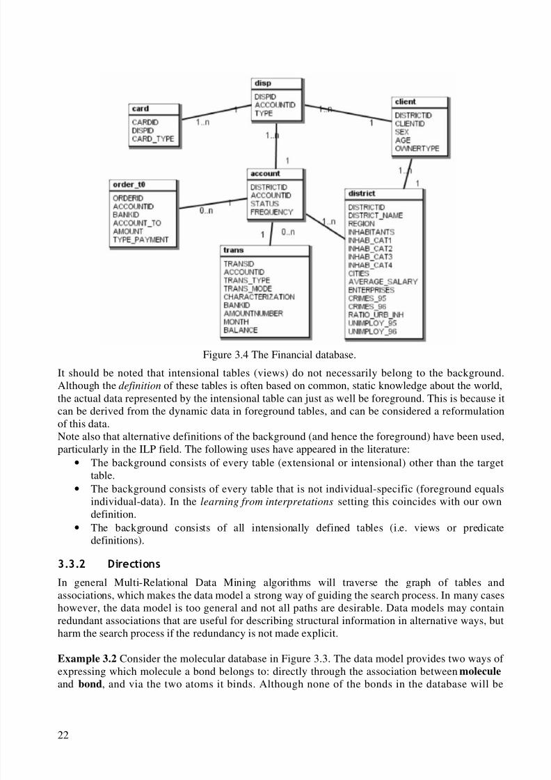
8/8/2019 Knobbe a.J. Multi-Relational Data Mining
http://slidepdf.com/reader/full/knobbe-aj-multi-relational-data-mining 33/129
22
Figure 3.4 The Financial database.
It should be noted that intensional tables (views) do not necessarily belong to the background.Although the definition of these tables is often based on common, static knowledge about the world,the actual data represented by the intensional table can just as well be foreground. This is because it
can be derived from the dynamic data in foreground tables, and can be considered a reformulationof this data.Note also that alternative definitions of the background (and hence the foreground) have been used,particularly in the ILP field. The following uses have appeared in the literature:
• The background consists of every table (extensional or intensional) other than the targettable.
• The background consists of every table that is not individual-specific (foreground equalsindividual-data). In the learning from interpretations setting this coincides with our owndefinition.
• The background consists of all intensionally defined tables (i.e. views or predicatedefinitions).
'LUHFWLRQV
In general Multi-Relational Data Mining algorithms will traverse the graph of tables andassociations, which makes the data model a strong way of guiding the search process. In many caseshowever, the data model is too general and not all paths are desirable. Data models may containredundant associations that are useful for describing structural information in alternative ways, butharm the search process if the redundancy is not made explicit.
Example 3.2 Consider the molecular database in Figure 3.3. The data model provides two ways of expressing which molecule a bond belongs to: directly through the association between molecule
and bond, and via the two atoms it binds. Although none of the bonds in the database will be
8/8/2019 Knobbe a.J. Multi-Relational Data Mining
http://slidepdf.com/reader/full/knobbe-aj-multi-relational-data-mining 34/129
23
associated with another molecule than the molecule its two atoms belong to, the data model doesnot exclude this. Therefore, the data model suggests patterns that are known to be impossible, andMDRM algorithms will waste time considering these patterns. The alternative paths in a data modelshould be explored during the search, but never together in the same pattern.
Directed associations are a good way to specify this extra declarative bias, as well as to furthercontrol the produced results. If an association between two tables is directed, the search process canonly introduce information in one table after the other table is introduced, in the direction of theassociation and not vice-versa. Directions can best be added in the following cases:
• redundant associations. An association is redundant if it represents a relation between twotables that is also represented by several other associations combined. The redundancy inExample 3.2 is solved by adding directions away from molecule.
• from foreground to background. In most cases it does not make sense to add structuralinformation to the static information in the background, hence the directional bias. In theFinancial dataset, we add directions to the associations connecting the demographic
information in district. As a further advantage, this will remove the only cycle in the datamodel.

8/8/2019 Knobbe a.J. Multi-Relational Data Mining
http://slidepdf.com/reader/full/knobbe-aj-multi-relational-data-mining 35/129
This page intentionally left blank
8/8/2019 Knobbe a.J. Multi-Relational Data Mining
http://slidepdf.com/reader/full/knobbe-aj-multi-relational-data-mining 36/129
25
0XOWL5HODWLRQDO3DWWHUQV
/RFDO6WUXFWXUH
It has become clear that individuals, and even more importantly groups of individuals, are the mainsubject of analysis in MRDM. Now that we know how individuals are represented in relational
databases, we should consider how to query databases of individuals, and select subgroups thatshare certain structural characteristics. In our MRDM framework we will mainly express suchstructural characteristics by building on conditions at the low level of relationships between pairs of tables. For example we will select candidate subgroups of molecules by extracting structuralfeatures from the molecule and the atom table and the association between them. We will refer tosuch incomplete and localised information as local structure. By combining conditions on the localstructure (not necessarily involving the target table) we end up with expressions about individuals.Local structure involves data in two tables, but more importantly, the association between them.The association will typically be one-to-many (or many-to-one depending on the order of the twotables). Such a one-to-many relationship basically defines a grouping on the records in the table onthe ‘many’ side, as demonstrated below:
We can select records in one table on the basis of features of the associated group of records in theother table. This way of extracting information about local structure by means of describing groupsof records will be the primary approach to building descriptions of individuals.There are two important ways of expressing conditions on groups in local structure. Choosing one
of these ways has a major impact on the pattern language to be used, and thus on the type of knowledge that can be extracted from the database. Furthermore, this choice determines the
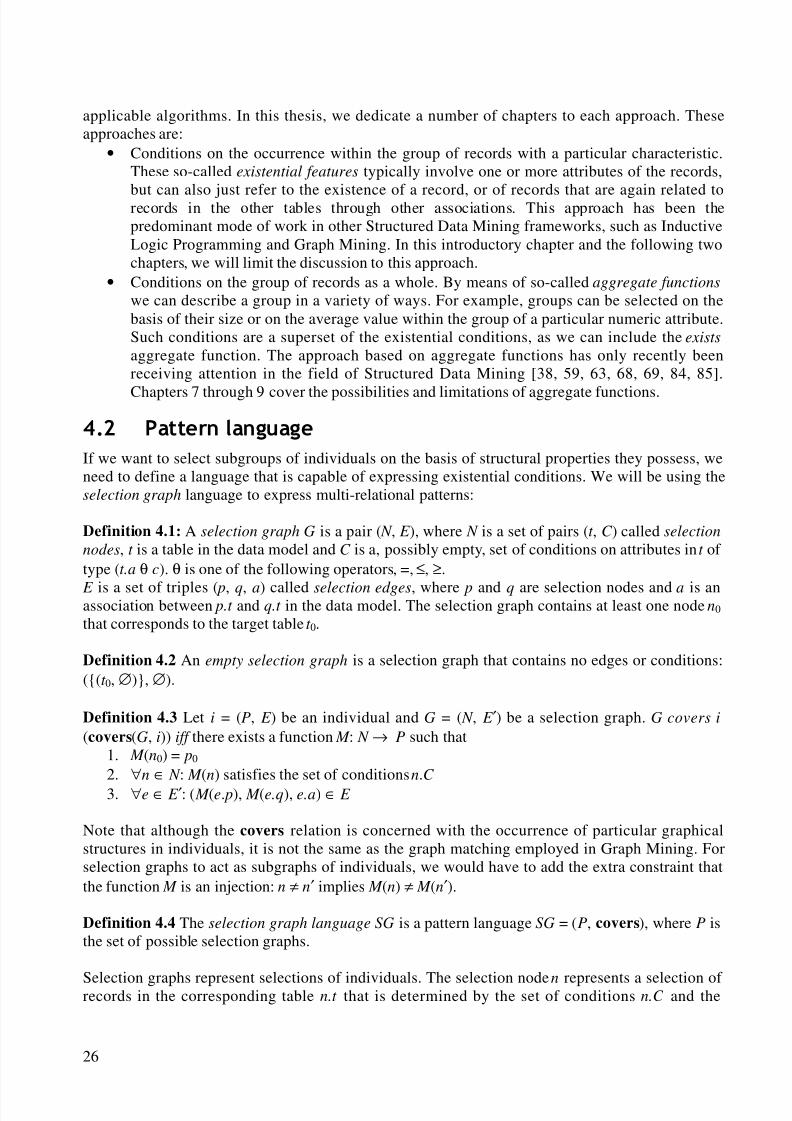
8/8/2019 Knobbe a.J. Multi-Relational Data Mining
http://slidepdf.com/reader/full/knobbe-aj-multi-relational-data-mining 37/129
26
applicable algorithms. In this thesis, we dedicate a number of chapters to each approach. Theseapproaches are:
• Conditions on the occurrence within the group of records with a particular characteristic.These so-called existential features typically involve one or more attributes of the records,
but can also just refer to the existence of a record, or of records that are again related torecords in the other tables through other associations. This approach has been thepredominant mode of work in other Structured Data Mining frameworks, such as InductiveLogic Programming and Graph Mining. In this introductory chapter and the following twochapters, we will limit the discussion to this approach.
• Conditions on the group of records as a whole. By means of so-called aggregate functions
we can describe a group in a variety of ways. For example, groups can be selected on thebasis of their size or on the average value within the group of a particular numeric attribute.Such conditions are a superset of the existential conditions, as we can include the exists
aggregate function. The approach based on aggregate functions has only recently beenreceiving attention in the field of Structured Data Mining [38, 59, 63, 68, 69, 84, 85].
Chapters 7 through 9 cover the possibilities and limitations of aggregate functions.
3DWWHUQODQJXDJH
If we want to select subgroups of individuals on the basis of structural properties they possess, weneed to define a language that is capable of expressing existential conditions. We will be using theselection graph language to express multi-relational patterns:
Definition 4.1: A selection graph G is a pair ( N , E ), where N is a set of pairs (t , C ) called selection
nodes, t is a table in the data model and C is a, possibly empty, set of conditions on attributes in t of type (t.a θ c). θ is one of the following operators, =, ≤, ≥.
E is a set of triples ( p, q, a) called selection edges, where p and q are selection nodes and a is anassociation between p.t and q.t in the data model. The selection graph contains at least one node n0
that corresponds to the target table t 0.
Definition 4.2 An empty selection graph is a selection graph that contains no edges or conditions:({(t 0, ∅)}, ∅).
Definition 4.3 Let i = (P, E ) be an individual and G = ( N , E ′) be a selection graph. G covers i
(covers(G, i)) iff there exists a function M : N → P such that1. M (n0) = p0
2. ∀n ∈ N : M (n) satisfies the set of conditions n.C
3. ∀e ∈ E ′: ( M (e. p), M (e.q), e.a) ∈ E
Note that although the covers relation is concerned with the occurrence of particular graphicalstructures in individuals, it is not the same as the graph matching employed in Graph Mining. Forselection graphs to act as subgraphs of individuals, we would have to add the extra constraint thatthe function M is an injection: n ≠ n′ implies M (n) ≠ M (n′).
Definition 4.4 The selection graph language SG is a pattern language SG = (P, covers), where P isthe set of possible selection graphs.
Selection graphs represent selections of individuals. The selection node n represents a selection of records in the corresponding table n.t that is determined by the set of conditions n.C and the
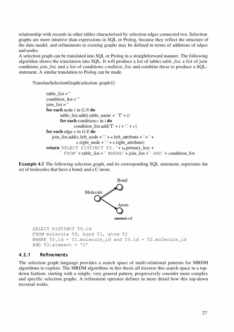
8/8/2019 Knobbe a.J. Multi-Relational Data Mining
http://slidepdf.com/reader/full/knobbe-aj-multi-relational-data-mining 38/129
27
relationship with records in other tables characterised by selection edges connected to n. Selectiongraphs are more intuitive than expressions in SQL or Prolog, because they reflect the structure of the data model, and refinements to existing graphs may be defined in terms of additions of edgesand nodes.
A selection graph can be translated into SQL or Prolog in a straightforward manner. The followingalgorithm shows the translation into SQL. It will produce a list of tables table_list , a list of joinconditions join_list , and a list of conditions condition_list , and combine these to produce a SQL-statement. A similar translation to Prolog can be made.
TranslateSelectionGraph(selection graph G)
table_list = ''condition_list = '' join_list = ''for each node i in G.N do
table_list.add(i.table_name + ' T' + i)for each condition c in i do
condition_list.add('T' + i + '.' + c)for each edge e in G.E do
join_list.add(e.left_node + '.' + e.left_attribute + ' = ' +e.right_node + '.' + e.right_attribute)
return 'SELECT DISTINCT T0. ' + t 0.primary_key +
' FROM ' + table_list + ' WHERE ' + join_list + ' AND ' + condition_list
Example 4.1 The following selection graph, and its corresponding SQL statement, represents theset of molecules that have a bond, and a C-atom.
SELECT DISTINCT T0.id
FROM molecule T0, bond T1, atom T2WHERE T0.id = T1.molecule_id and T0.id = T2.molecule_id
AND T2.element = 'C'
5HILQHPHQWV
The selection graph language provides a search space of multi-relational patterns for MRDMalgorithms to explore. The MRDM algorithms in this thesis all traverse this search space in a top-down fashion: starting with a simple, very general pattern, progressively consider more complexand specific selection graphs. A refinement operator defines in more detail how this top-downtraversal works.
Atom
Molecule
Bond
element = C
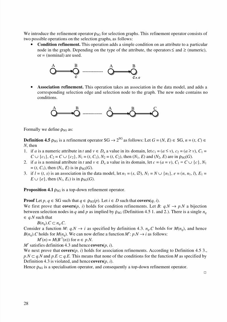
8/8/2019 Knobbe a.J. Multi-Relational Data Mining
http://slidepdf.com/reader/full/knobbe-aj-multi-relational-data-mining 39/129
28
A B
C ∧∧∧∧ c
A B
C
A B A B C
We introduce the refinement operator ρSG for selection graphs. This refinement operator consists of two possible operations on the selection graphs, as follows:
• Condition refinement. This operation adds a simple condition on an attribute to a particularnode in the graph. Depending on the type of the attribute, the operators ≤ and ≥ (numeric),
or = (nominal) are used.
• Association refinement. This operation takes an association in the data model, and adds acorresponding selection edge and selection node to the graph. The new node contains noconditions.
Formally we define ρSG as:
Definition 4.5 ρSG is a refinement operator SG → 2SG as follows: Let G = ( N , E ) ∈ SG, n = (t , C ) ∈ N , then1. if a is a numeric attribute in t and v ∈ Da a value in its domain, let c1 = (a ≤ v), c2 = (a ≥ v), C 1 =
C ∪ {c1}, C 2 = C ∪ {c2}, N 1 = (t , C 1), N 2 = (t , C 2), then ( N 1, E ) and ( N 2, E ) are in ρSG(G).2. if a is a nominal attribute in t and v ∈ Da a value in its domain, let c = (a = v), C 1 = C ∪ {c}, N 1
= (t , C 1), then ( N 1, E ) is in ρSG(G).3. if l = (t , s) is an association in the data model, let n1 = (s, ∅), N 1 = N ∪ {n1}, e = (n, n1, l), E 1 = E ∪ {e}, then ( N 1, E 1) is in ρSG(G).
Proposition 4.1 ρSG is a top-down refinement operator.
Proof Let p, q ∈ SG such that q ∈ ρSG( p). Let i ∈ D such that covers(q, i).We first prove that covers( p, i) holds for condition refinements. Let B: q. N → p. N a bijectionbetween selection nodes in q and p as implied by ρSG (Definition 4.5 1. and 2.). There is a single nq
∈ q.N such that B(nq).C ⊂ nq.C .
Consider a function M : q. N → i as specified by definition 4.3. nq.C holds for M (nq), and hence B(nq).C holds for M (nq). We can now define a function M ′: p. N → i as follows:
M ′(n) = M ( B-1(n)) for n ∈ p. N . M ′ satisfies definition 4.3 and hence covers( p, i).We next prove that covers( p, i) holds for association refinements. According to Definition 4.5 3., p.N ⊂ q.N and p.E ⊂ q.E. This means that none of the conditions for the function M as specified byDefinition 4.3 is violated, and hence covers( p, i).Hence ρSG is a specialisation operator, and consequently a top-down refinement operator.
8/8/2019 Knobbe a.J. Multi-Relational Data Mining
http://slidepdf.com/reader/full/knobbe-aj-multi-relational-data-mining 40/129
29
It should be noted that only tree-structured selection graphs can be derived from the empty selectiongraph. The refinement operator will never produce a cycle in the graph. As such, ρSG is notcomplete: some patterns in SG cannot be derived. Although a single refinement can be added tomake ρSG complete, we have chosen to restrict ourselves to tree-structured graphs. Later extensions
of SG will make cycles troublesome (see Chapters 6, 9 and 10). 3DWWHUQ&RPSOH[LW\
In the remainder of this thesis, we will be presenting a number of MRDM techniques thatmanipulate selection graphs. In order to judge the power and limitations of these techniques, wewill consider the complexity of the multi-relational patterns they are able to discover. The followingmeasures of complexity for selection graphs will be helpful:
Definition 4.6
1. association-depth: da(G) equals the length of the longest path starting at the root-node in G.2. refinement-depth: dr(G) equals the sum of the number of edges and conditions in G.
3. association-width: wa(G) equals the largest sum of the number of conditions and childrenper node, not including the root-node.
The intuition of these definitions is as follows. An algorithm searches association-deep if pieces of discovered substructure are refined by adding more substructure, which results in chains of edges inselection graphs. With each new association, information from a new table is involved. Analgorithm searches refinement-deep if it considers very specific patterns, regardless of the numberof tables involved. The refinement-depth of a selection graph corresponds to the number of consecutive refinements necessary to derive the graph from the empty graph. Even propositionalalgorithms may produce refinement-deep patterns that contain many conditions at the root-node andno other nodes. Rather than long chains of associations, association-wide algorithms are concernedwith the frequent reuse of a single association. If information from a new table is included, it will befurther refined by extra restrictions, either through conditions on this information or through furtherlocal structure.
Example 4.2 The measures produce the following complexity characteristics for the selection graphpresented in Example 4.1:
da(G) = 1, dr(G) = 3, wa(G) = 1
&KDUDFWHULVWLFVRI0XOWL5HODWLRQDO3DWWHUQVAnalysing local structure by means of existential features over groups has a number of characteristics that set it apart from what one might be used to in Propositional Data Mining. Thesepeculiarities of MRDM are important because of their impact on the design of MRDM algorithms.They are also important when interpreting correctly the output of algorithms. We summarise themost crucial ones. Note that these characteristics derive directly from predicate logic:
• Refinements may not always produce patterns with a lower coverage. This is especially truefor association refinements, where nodes that are totally redundant may be added to aselection graph. This redundancy is the result of declarative bias that indicates that there willalways be a part corresponding to the new node. In our molecular example, simply adding a
new atom-node through the association between atom and molecule does not logicallychange the pattern at hand, as all molecules must contain atoms. Although such irrelevant
8/8/2019 Knobbe a.J. Multi-Relational Data Mining
http://slidepdf.com/reader/full/knobbe-aj-multi-relational-data-mining 41/129
30
nodes produce no immediate benefit, they are essential because they may be the startingpoint for further refinements.
• Associations will often appear multiple times as edges from a single node in a selectiongraph. This indicates that parts with different characteristics, but of the same class, are
required to appear. These different sets of characteristics need not be mutually exclusive.They may appear in a single part. Multiple edges of the same association only make sense(and should be allowed as refinements) if the data model indicates a one-to-manyrelationship.
• In Data Mining, it is often desirable to split a particular subgroup into mutually exclusivesubgroups, for example to build hierarchical models of the data, such as decision trees. InPropositional Data Mining, this can be done for example on the basis of the values of anominal attribute. Each value represents a subgroup, and the union of subgroups thusformed represents the original subgroup. There is no overlap between subgroups, so the sizeof the original subgroup equals the sum of the sizes of the splits. This simple and attractivefeature does not hold for splits on nominal attributes in MRDM. Due to the one-to-many
associations and the existential nature of conditions, individuals will often exhibit multiplevalues for the nominal attribute at the same time. This will place individuals in multiplesubgroups represented by the nominal values, causing overlap, and thus problems withadding sizes. In general, nominal attributes can only be used to form true splits if they occurin the target table. As a resulting effect, it is often not possible to use the distribution of values in the nominal attribute to predict the size of subgroups. For example, if we list allatoms in a database of organic compounds, we notice that hydrogen atoms occur more oftenthan carbon atoms. However, if we use these values to produce subgroups, we notice thatboth subgroups are equal. In fact, all organic molecules (in this case) contain both carbonand hydrogen.
• A similar effect occurs with numeric splits. The intuition from PDM is that as one changes
the numeric threshold to increasing values as they occur in the numeric attributes, the size of the resulting subgroup will either monotonically increase or decrease. In MRDM however,often only a few of the encountered values will actually be proper thresholds. Of all thenumeric values occurring within a single individual, only the minimum and maximum arevalid as thresholds to in- or exclude the individual. Handling numeric data is covered inSection 4.4.
• As a corollary of the previous two effects, it should be noted that complementary operators,such as = and , or < and , do not generally produce complementary subgroups. This isclear if we think of the two operators as representing the two values of a binary attribute,which is a special case of a nominal attribute. Each operator should be consideredindependently. For numeric attributes, each inequality operator should be treated separately,together with separate sets of valid thresholds. See again Section 4.4.
• The most obscure peculiarity of MRDM has to do with interactions between multipleconditions. An interesting effect of this is that two conditions may be irrelevant in isolation,whereas combined they do produce a proper refinement. This is demonstrated by thedatabase in Figure 4.1. The database describes two hands of playing cards. If we query thisdatabase for suit = , we obtain two hands. Two hands are also obtained if queried for rank
= A. We would expect the conjunction of these conditions to produce the same result, asboth conditions appear not to be selective. However, there is only a single hand with suit =
∧ rank = A. This example shows how a refinement may change (beneficially or not) theusefulness of a prior refinement, thus producing interactions between conditions. One way
to understand this is to look at conditions not just as selections on the level of individuals,
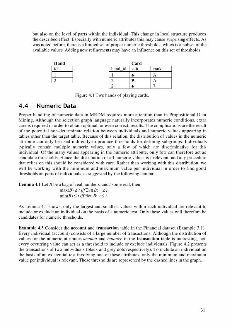
8/8/2019 Knobbe a.J. Multi-Relational Data Mining
http://slidepdf.com/reader/full/knobbe-aj-multi-relational-data-mining 42/129
31
but also on the level of parts within the individual. This change in local structure producesthe described effect. Especially with numeric attributes this may cause surprising effects. Aswas noted before, there is a limited set of proper numeric thresholds, which is a subset of theavailable values. Adding new refinements may have an influence on this set of thresholds.
Figure 4.1 Two hands of playing cards.
1XPHULF'DWD
Proper handling of numeric data in MRDM requires more attention than in Propositional DataMining. Although the selection graph language naturally incorporates numeric conditions, extracare is required in order to obtain optimal, or even correct, results. The complications are the resultof the potential non-determinate relation between individuals and numeric values appearing intables other than the target table. Because of this relation, the distribution of values in the numericattribute can only be used indirectly to produce thresholds for defining subgroups. Individualstypically contain multiple numeric values, only a few of which are discriminative for thisindividual. Of the many values appearing in the numeric attribute, only few can therefore act ascandidate thresholds. Hence the distribution of all numeric values is irrelevant, and any procedurethat relies on this should be considered with care. Rather than working with this distribution, wewill be working with the minimum and maximum value per individual in order to find good
thresholds on parts of individuals, as suggested by the following lemma:
Lemma 4.1 Let B be a bag of real numbers, and t some real, thenmax( B) ≥ t iff ∃v∈ B: v ≥ t ,min( B) ≤ t iff ∃v∈ B: v ≤ t .
As Lemma 4.1 shows, only the largest and smallest values within each individual are relevant toinclude or exclude an individual on the basis of a numeric test. Only these values will therefore becandidates for numeric thresholds.
Example 4.3 Consider the account and transaction table in the Financial dataset (Example 3.1).Every individual (account) consists of a large number of transactions. Although the distribution of values for the numeric attributes amount and balance in the transaction table is interesting, notevery occurring value can act as a threshold to include or exclude individuals. Figure 4.2 presentsthe transactions of two individuals (black and grey dots respectively). To include an individual onthe basis of an existential test involving one of these attributes, only the minimum and maximumvalue per individual is relevant. These thresholds are represented by the dashed lines in the graph.
Hand Card
id hand_id suit rank1 1 A2 2 A
2 7
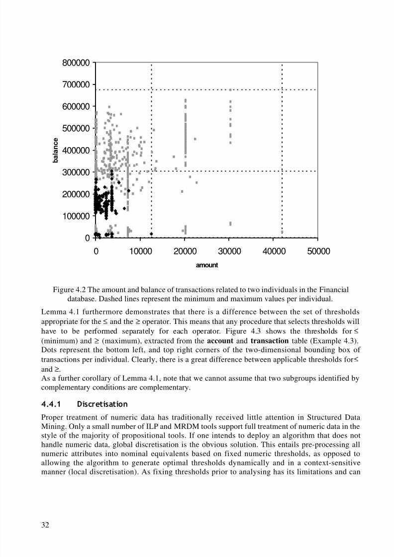
8/8/2019 Knobbe a.J. Multi-Relational Data Mining
http://slidepdf.com/reader/full/knobbe-aj-multi-relational-data-mining 43/129
32
0
100000
200000
300000
400000
500000
600000
700000
800000
0 10000 20000 30000 40000 50000
amount
b a l a n c e
Figure 4.2 The amount and balance of transactions related to two individuals in the Financialdatabase. Dashed lines represent the minimum and maximum values per individual.
Lemma 4.1 furthermore demonstrates that there is a difference between the set of thresholdsappropriate for the ≤ and the ≥ operator. This means that any procedure that selects thresholds willhave to be performed separately for each operator. Figure 4.3 shows the thresholds for ≤(minimum) and ≥ (maximum), extracted from the account and transaction table (Example 4.3).Dots represent the bottom left, and top right corners of the two-dimensional bounding box of transactions per individual. Clearly, there is a great difference between applicable thresholds for ≤and ≥.As a further corollary of Lemma 4.1, note that we cannot assume that two subgroups identified by
complementary conditions are complementary. 'LVFUHWLVDWLRQ
Proper treatment of numeric data has traditionally received little attention in Structured DataMining. Only a small number of ILP and MRDM tools support full treatment of numeric data in thestyle of the majority of propositional tools. If one intends to deploy an algorithm that does nothandle numeric data, global discretisation is the obvious solution. This entails pre-processing allnumeric attributes into nominal equivalents based on fixed numeric thresholds, as opposed toallowing the algorithm to generate optimal thresholds dynamically and in a context-sensitivemanner (local discretisation). As fixing thresholds prior to analysing has its limitations and can
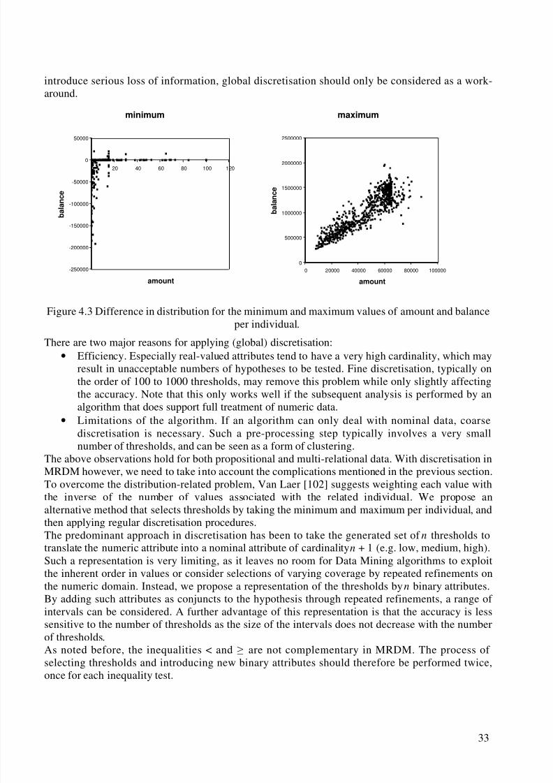
8/8/2019 Knobbe a.J. Multi-Relational Data Mining
http://slidepdf.com/reader/full/knobbe-aj-multi-relational-data-mining 44/129
33
introduce serious loss of information, global discretisation should only be considered as a work-around.
minimum
-250000
-200000
-150000
-100000
-50000
0
50000
0 20 40 60 80 100 120
amount
b a l a n c e
maximum
0
500000
1000000
1500000
2000000
2500000
0 20000 40000 60000 80000 100000
amount
b a l a n c e
Figure 4.3 Difference in distribution for the minimum and maximum values of amount and balanceper individual.
There are two major reasons for applying (global) discretisation:• Efficiency. Especially real-valued attributes tend to have a very high cardinality, which may
result in unacceptable numbers of hypotheses to be tested. Fine discretisation, typically onthe order of 100 to 1000 thresholds, may remove this problem while only slightly affectingthe accuracy. Note that this only works well if the subsequent analysis is performed by an
algorithm that does support full treatment of numeric data.• Limitations of the algorithm. If an algorithm can only deal with nominal data, coarsediscretisation is necessary. Such a pre-processing step typically involves a very smallnumber of thresholds, and can be seen as a form of clustering.
The above observations hold for both propositional and multi-relational data. With discretisation inMRDM however, we need to take into account the complications mentioned in the previous section.To overcome the distribution-related problem, Van Laer [102] suggests weighting each value withthe inverse of the number of values associated with the related individual. We propose analternative method that selects thresholds by taking the minimum and maximum per individual, andthen applying regular discretisation procedures.The predominant approach in discretisation has been to take the generated set of n thresholds to
translate the numeric attribute into a nominal attribute of cardinality n + 1 (e.g. low, medium, high).Such a representation is very limiting, as it leaves no room for Data Mining algorithms to exploitthe inherent order in values or consider selections of varying coverage by repeated refinements onthe numeric domain. Instead, we propose a representation of the thresholds by n binary attributes.By adding such attributes as conjuncts to the hypothesis through repeated refinements, a range of intervals can be considered. A further advantage of this representation is that the accuracy is lesssensitive to the number of thresholds as the size of the intervals does not decrease with the numberof thresholds.As noted before, the inequalities < and are not complementary in MRDM. The process of selecting thresholds and introducing new binary attributes should therefore be performed twice,once for each inequality test.

8/8/2019 Knobbe a.J. Multi-Relational Data Mining
http://slidepdf.com/reader/full/knobbe-aj-multi-relational-data-mining 45/129
34
Example 4.4 Consider the order table in the Financial dataset. The amount attribute can bediscretised with the respect to the target table account as follows. For the operator we canintroduce three thresholds (1000, 2800 and 4720) which divide the accounts up into four subgroupsof roughly equal coverage. These thresholds produce three new attributes in order (amountlow1 =
(amount 1000) etc.). This process is repeated with thresholds 7820, 5850 and 4000 for the operator, to form attributes amounthigh1 etc. These thresholds produce a similar equal-coveragedivision, although generally not with the same subgroups. Note how MRDM algorithms canconsider subgroups of 75%, 50% and 25% of the accounts in two ways, or go through thesesubgroups in progressive refinements by adding conditions on the binary attributes.
8/8/2019 Knobbe a.J. Multi-Relational Data Mining
http://slidepdf.com/reader/full/knobbe-aj-multi-relational-data-mining 46/129
35
0XOWL5HODWLRQDO5XOH'LVFRYHU\
In this chapter, we take a common Data Mining task, known as Rule Discovery, and show how itcan be approached in a multi-relational setting. Rule discovery is concerned with producing acollection of regularities from a given database. As the name suggests, the regularities take the formof rules. In this case, we present an algorithm that finds rules with a previously specifiedconclusion, as follows:
ST
where S is an interesting subgroup identified by a selection graph, and T is a subgroup identified bya simple propositional condition on the target table that is fixed (the target ). Rules are local models:they specify some knowledge about the individuals covered by S, but not about the remainder of thedatabase. The rules that are reported are independent. They simply express a regularity of sufficientinterest, regardless of other rules that may express (partially) similar results. As such, the collectionof rules should not be treated as a classifier: not all conceivable individuals may be covered, andsome individuals may be covered by multiple (competing) rules.
5XOH'LVFRYHU\
Our rule discovery algorithm follows the generic Data Mining algorithm outline, as proposed byHand, Mannila and Smyth [43]. This generic algorithm is centred around a top-down searchalgorithm with five variables:
• The data mining task that is addressed.• The structure (functional form) of the model considered.• The score function used to judge candidate models.• The search strategy employed to traverse the space of models.• The data management technique used for storing, indexing and retrieving data.
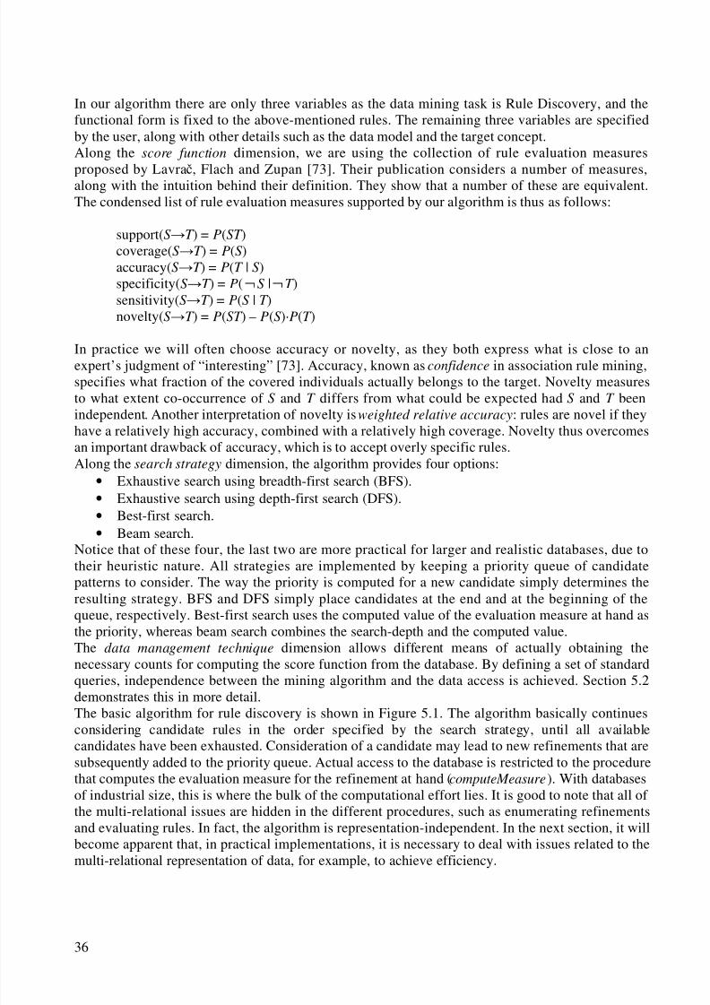
8/8/2019 Knobbe a.J. Multi-Relational Data Mining
http://slidepdf.com/reader/full/knobbe-aj-multi-relational-data-mining 47/129
36
In our algorithm there are only three variables as the data mining task is Rule Discovery, and thefunctional form is fixed to the above-mentioned rules. The remaining three variables are specifiedby the user, along with other details such as the data model and the target concept.Along the score function dimension, we are using the collection of rule evaluation measures
proposed by Lavraþ, Flach and Zupan [73]. Their publication considers a number of measures,along with the intuition behind their definition. They show that a number of these are equivalent.The condensed list of rule evaluation measures supported by our algorithm is thus as follows:
support(ST ) = P(ST )coverage(ST ) = P(S)accuracy(ST ) = P(T | S)specificity(ST ) = P( ¬ S | ¬ T )sensitivity(ST ) = P(S | T )novelty(ST ) = P(ST ) – P(S)·P(T )
In practice we will often choose accuracy or novelty, as they both express what is close to anexpert’s judgment of “interesting” [73]. Accuracy, known as confidence in association rule mining,specifies what fraction of the covered individuals actually belongs to the target. Novelty measuresto what extent co-occurrence of S and T differs from what could be expected had S and T beenindependent. Another interpretation of novelty is weighted relative accuracy: rules are novel if theyhave a relatively high accuracy, combined with a relatively high coverage. Novelty thus overcomesan important drawback of accuracy, which is to accept overly specific rules.Along the search strategy dimension, the algorithm provides four options:
• Exhaustive search using breadth-first search (BFS).• Exhaustive search using depth-first search (DFS).• Best-first search.
• Beam search.Notice that of these four, the last two are more practical for larger and realistic databases, due totheir heuristic nature. All strategies are implemented by keeping a priority queue of candidatepatterns to consider. The way the priority is computed for a new candidate simply determines theresulting strategy. BFS and DFS simply place candidates at the end and at the beginning of thequeue, respectively. Best-first search uses the computed value of the evaluation measure at hand asthe priority, whereas beam search combines the search-depth and the computed value.The data management technique dimension allows different means of actually obtaining thenecessary counts for computing the score function from the database. By defining a set of standardqueries, independence between the mining algorithm and the data access is achieved. Section 5.2demonstrates this in more detail.The basic algorithm for rule discovery is shown in Figure 5.1. The algorithm basically continuesconsidering candidate rules in the order specified by the search strategy, until all availablecandidates have been exhausted. Consideration of a candidate may lead to new refinements that aresubsequently added to the priority queue. Actual access to the database is restricted to the procedurethat computes the evaluation measure for the refinement at hand (computeMeasure). With databasesof industrial size, this is where the bulk of the computational effort lies. It is good to note that all of the multi-relational issues are hidden in the different procedures, such as enumerating refinementsand evaluating rules. In fact, the algorithm is representation-independent. In the next section, it willbecome apparent that, in practical implementations, it is necessary to deal with issues related to themulti-relational representation of data, for example, to achieve efficiency.
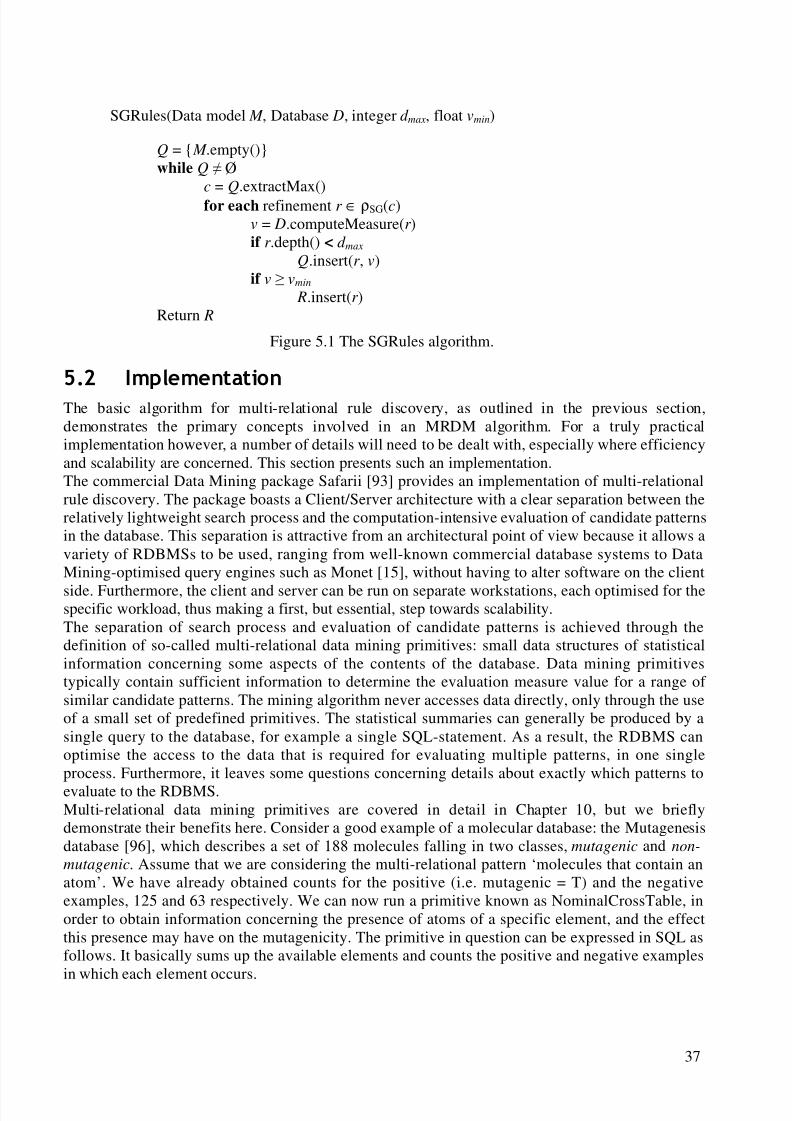
8/8/2019 Knobbe a.J. Multi-Relational Data Mining
http://slidepdf.com/reader/full/knobbe-aj-multi-relational-data-mining 48/129
37
SGRules(Data model M , Database D, integer d max, float vmin)
Q = { M .empty()}while Q Ø
c = Q.extractMax()for each refinement r ∈ ρSG(c)
v = D.computeMeasure(r )if r .depth() < d max
Q.insert(r , v)if v vmin
R.insert(r )Return R
Figure 5.1 The SGRules algorithm.
,PSOHPHQWDWLRQ
The basic algorithm for multi-relational rule discovery, as outlined in the previous section,demonstrates the primary concepts involved in an MRDM algorithm. For a truly practicalimplementation however, a number of details will need to be dealt with, especially where efficiencyand scalability are concerned. This section presents such an implementation.The commercial Data Mining package Safarii [93] provides an implementation of multi-relationalrule discovery. The package boasts a Client/Server architecture with a clear separation between therelatively lightweight search process and the computation-intensive evaluation of candidate patternsin the database. This separation is attractive from an architectural point of view because it allows avariety of RDBMSs to be used, ranging from well-known commercial database systems to DataMining-optimised query engines such as Monet [15], without having to alter software on the client
side. Furthermore, the client and server can be run on separate workstations, each optimised for thespecific workload, thus making a first, but essential, step towards scalability.The separation of search process and evaluation of candidate patterns is achieved through thedefinition of so-called multi-relational data mining primitives: small data structures of statisticalinformation concerning some aspects of the contents of the database. Data mining primitivestypically contain sufficient information to determine the evaluation measure value for a range of similar candidate patterns. The mining algorithm never accesses data directly, only through the useof a small set of predefined primitives. The statistical summaries can generally be produced by asingle query to the database, for example a single SQL-statement. As a result, the RDBMS canoptimise the access to the data that is required for evaluating multiple patterns, in one singleprocess. Furthermore, it leaves some questions concerning details about exactly which patterns toevaluate to the RDBMS.Multi-relational data mining primitives are covered in detail in Chapter 10, but we brieflydemonstrate their benefits here. Consider a good example of a molecular database: the Mutagenesisdatabase [96], which describes a set of 188 molecules falling in two classes, mutagenic and non-
mutagenic. Assume that we are considering the multi-relational pattern ‘molecules that contain anatom’. We have already obtained counts for the positive (i.e. mutagenic = T) and the negativeexamples, 125 and 63 respectively. We can now run a primitive known as NominalCrossTable, inorder to obtain information concerning the presence of atoms of a specific element, and the effectthis presence may have on the mutagenicity. The primitive in question can be expressed in SQL asfollows. It basically sums up the available elements and counts the positive and negative examplesin which each element occurs.
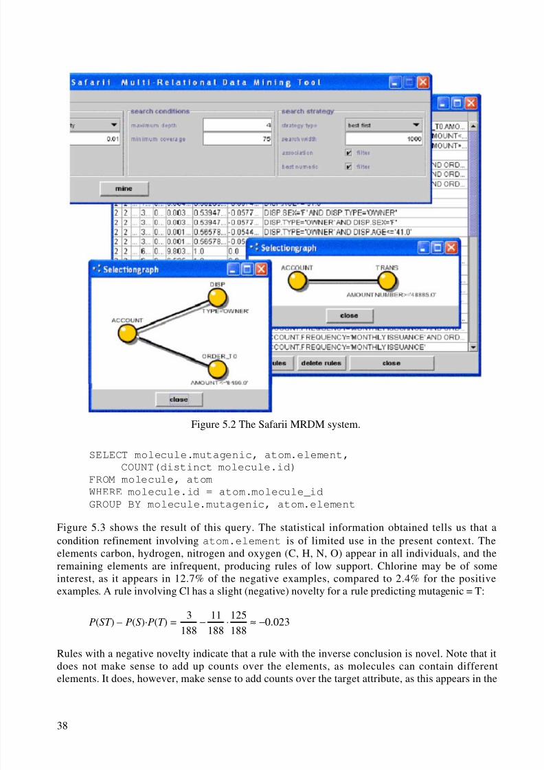
8/8/2019 Knobbe a.J. Multi-Relational Data Mining
http://slidepdf.com/reader/full/knobbe-aj-multi-relational-data-mining 49/129
38
Figure 5.2 The Safarii MRDM system.
SELECT molecule.mutagenic, atom.element,
COUNT(distinct molecule.id)
FROM molecule, atom
WHERE molecule.id = atom.molecule_id
GROUP BY molecule.mutagenic, atom.element
Figure 5.3 shows the result of this query. The statistical information obtained tells us that a
condition refinement involving atom.element is of limited use in the present context. Theelements carbon, hydrogen, nitrogen and oxygen (C, H, N, O) appear in all individuals, and theremaining elements are infrequent, producing rules of low support. Chlorine may be of someinterest, as it appears in 12.7% of the negative examples, compared to 2.4% for the positiveexamples. A rule involving Cl has a slight (negative) novelty for a rule predicting mutagenic = T:
P(ST ) – P(S)·P(T ) = 023.0188
125
188
11
188
3−≈⋅−
Rules with a negative novelty indicate that a rule with the inverse conclusion is novel. Note that itdoes not make sense to add up counts over the elements, as molecules can contain differentelements. It does, however, make sense to add counts over the target attribute, as this appears in the
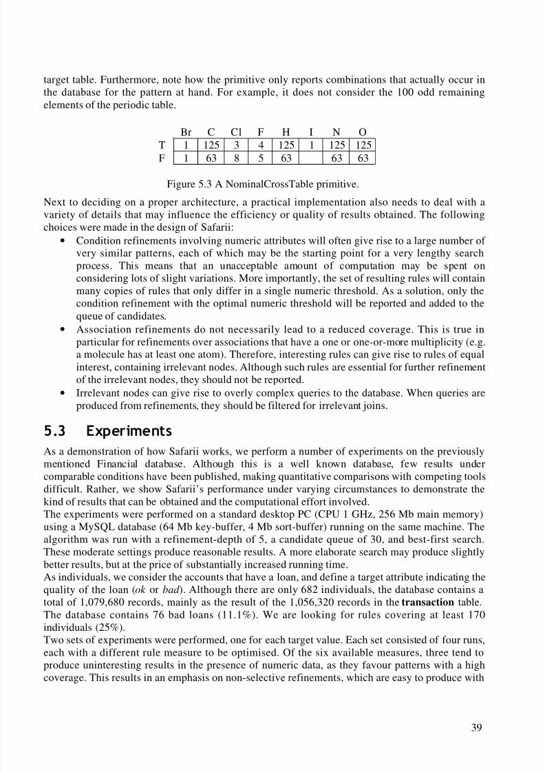
8/8/2019 Knobbe a.J. Multi-Relational Data Mining
http://slidepdf.com/reader/full/knobbe-aj-multi-relational-data-mining 50/129
39
target table. Furthermore, note how the primitive only reports combinations that actually occur inthe database for the pattern at hand. For example, it does not consider the 100 odd remainingelements of the periodic table.
Figure 5.3 A NominalCrossTable primitive.
Next to deciding on a proper architecture, a practical implementation also needs to deal with avariety of details that may influence the efficiency or quality of results obtained. The followingchoices were made in the design of Safarii:
• Condition refinements involving numeric attributes will often give rise to a large number of very similar patterns, each of which may be the starting point for a very lengthy search
process. This means that an unacceptable amount of computation may be spent onconsidering lots of slight variations. More importantly, the set of resulting rules will containmany copies of rules that only differ in a single numeric threshold. As a solution, only thecondition refinement with the optimal numeric threshold will be reported and added to thequeue of candidates.
• Association refinements do not necessarily lead to a reduced coverage. This is true inparticular for refinements over associations that have a one or one-or-more multiplicity (e.g.a molecule has at least one atom). Therefore, interesting rules can give rise to rules of equalinterest, containing irrelevant nodes. Although such rules are essential for further refinementof the irrelevant nodes, they should not be reported.
• Irrelevant nodes can give rise to overly complex queries to the database. When queries are
produced from refinements, they should be filtered for irrelevant joins.
([SHULPHQWV
As a demonstration of how Safarii works, we perform a number of experiments on the previouslymentioned Financial database. Although this is a well known database, few results undercomparable conditions have been published, making quantitative comparisons with competing toolsdifficult. Rather, we show Safarii’s performance under varying circumstances to demonstrate thekind of results that can be obtained and the computational effort involved.The experiments were performed on a standard desktop PC (CPU 1 GHz, 256 Mb main memory)using a MySQL database (64 Mb key-buffer, 4 Mb sort-buffer) running on the same machine. The
algorithm was run with a refinement-depth of 5, a candidate queue of 30, and best-first search.These moderate settings produce reasonable results. A more elaborate search may produce slightlybetter results, but at the price of substantially increased running time.As individuals, we consider the accounts that have a loan, and define a target attribute indicating thequality of the loan (ok or bad ). Although there are only 682 individuals, the database contains atotal of 1,079,680 records, mainly as the result of the 1,056,320 records in the transaction table.The database contains 76 bad loans (11.1%). We are looking for rules covering at least 170individuals (25%).Two sets of experiments were performed, one for each target value. Each set consisted of four runs,each with a different rule measure to be optimised. Of the six available measures, three tend toproduce uninteresting results in the presence of numeric data, as they favour patterns with a high
coverage. This results in an emphasis on non-selective refinements, which are easy to produce with
Br C Cl F H I N OT 1 125 3 4 125 1 125 125F 1 63 8 5 63 63 63
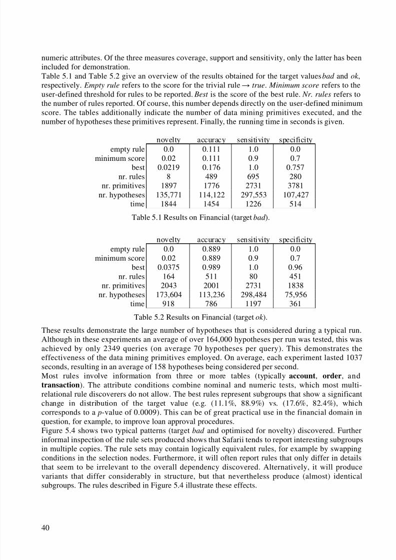
8/8/2019 Knobbe a.J. Multi-Relational Data Mining
http://slidepdf.com/reader/full/knobbe-aj-multi-relational-data-mining 51/129
40
numeric attributes. Of the three measures coverage, support and sensitivity, only the latter has beenincluded for demonstration.Table 5.1 and Table 5.2 give an overview of the results obtained for the target values bad and ok ,respectively. Empty rule refers to the score for the trivial rule true. Minimum score refers to the
user-defined threshold for rules to be reported. Best is the score of the best rule. Nr. rules refers tothe number of rules reported. Of course, this number depends directly on the user-defined minimumscore. The tables additionally indicate the number of data mining primitives executed, and thenumber of hypotheses these primitives represent. Finally, the running time in seconds is given.
novelty accuracy sensitivity specificityempty rule 0.0 0.111 1.0 0.0
minimum score 0.02 0.111 0.9 0.7best 0.0219 0.176 1.0 0.757
nr. rules 8 489 695 280nr. primitives 1897 1776 2731 3781
nr. hypotheses 135,771 114,122 297,553 107,427time 1844 1454 1226 514
Table 5.1 Results on Financial (target bad ).
novelty accuracy sensitivity specificityempty rule 0.0 0.889 1.0 0.0
minimum score 0.02 0.889 0.9 0.7best 0.0375 0.989 1.0 0.96
nr. rules 164 511 80 451nr. primitives 2043 2001 2731 1838
nr. hypotheses 173,604 113,236 298,484 75,956time 918 786 1197 361
Table 5.2 Results on Financial (target ok ).
These results demonstrate the large number of hypotheses that is considered during a typical run.Although in these experiments an average of over 164,000 hypotheses per run was tested, this wasachieved by only 2349 queries (on average 70 hypotheses per query). This demonstrates theeffectiveness of the data mining primitives employed. On average, each experiment lasted 1037seconds, resulting in an average of 158 hypotheses being considered per second.Most rules involve information from three or more tables (typically account, order, andtransaction). The attribute conditions combine nominal and numeric tests, which most multi-
relational rule discoverers do not allow. The best rules represent subgroups that show a significantchange in distribution of the target value (e.g. (11.1%, 88.9%) vs. (17.6%, 82.4%), whichcorresponds to a p-value of 0.0009). This can be of great practical use in the financial domain inquestion, for example, to improve loan approval procedures.Figure 5.4 shows two typical patterns (target bad and optimised for novelty) discovered. Furtherinformal inspection of the rule sets produced shows that Safarii tends to report interesting subgroupsin multiple copies. The rule sets may contain logically equivalent rules, for example by swappingconditions in the selection nodes. Furthermore, it will often report rules that only differ in detailsthat seem to be irrelevant to the overall dependency discovered. Alternatively, it will producevariants that differ considerably in structure, but that nevertheless produce (almost) identicalsubgroups. The rules described in Figure 5.4 illustrate these effects.
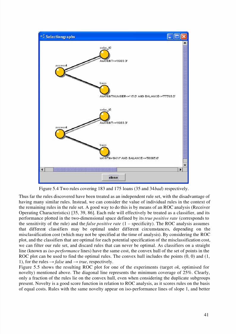
8/8/2019 Knobbe a.J. Multi-Relational Data Mining
http://slidepdf.com/reader/full/knobbe-aj-multi-relational-data-mining 52/129
41
Figure 5.4 Two rules covering 183 and 175 loans (35 and 34 bad ) respectively.
Thus far the rules discovered have been treated as an independent rule set, with the disadvantage of having many similar rules. Instead, we can consider the value of individual rules in the context of the remaining rules in the rule set. A good way to do this is by means of an ROC analysis (ReceiverOperating Characteristics) [35, 39, 86]. Each rule will effectively be treated as a classifier, and itsperformance plotted in the two-dimensional space defined by its true positive rate (corresponds tothe sensitivity of the rule) and the false positive rate (1 – specificity). The ROC analysis assumesthat different classifiers may be optimal under different circumstances, depending on the
misclassification cost (which may not be specified at the time of analysis). By considering the ROCplot, and the classifiers that are optimal for each potential specification of the misclassification cost,we can filter our rule set, and discard rules that can never be optimal. As classifiers on a straightline (known as iso-performance lines) have the same cost, the convex hull of the set of points in theROC plot can be used to find the optimal rules. The convex hull includes the points (0, 0) and (1,1), for the rules false and true, respectively.Figure 5.5 shows the resulting ROC plot for one of the experiments (target ok , optimised fornovelty) mentioned above. The diagonal line represents the minimum coverage of 25%. Clearly,only a fraction of the rules lie on the convex hull, even when considering the duplicate subgroupspresent. Novelty is a good score function in relation to ROC analysis, as it scores rules on the basisof equal costs. Rules with the same novelty appear on iso-performance lines of slope 1, and better
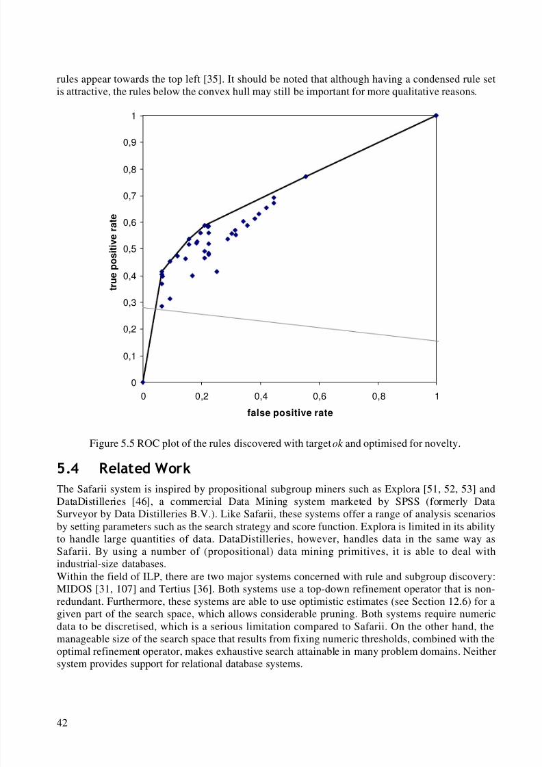
8/8/2019 Knobbe a.J. Multi-Relational Data Mining
http://slidepdf.com/reader/full/knobbe-aj-multi-relational-data-mining 53/129
42
rules appear towards the top left [35]. It should be noted that although having a condensed rule setis attractive, the rules below the convex hull may still be important for more qualitative reasons.
0
0,1
0,2
0,3
0,4
0,5
0,6
0,7
0,8
0,9
1
0 0,2 0,4 0,6 0,8 1
false positive rate
t r u e p
o s i t i v e
r a t e
Figure 5.5 ROC plot of the rules discovered with target ok and optimised for novelty.
5HODWHG:RUN
The Safarii system is inspired by propositional subgroup miners such as Explora [51, 52, 53] andDataDistilleries [46], a commercial Data Mining system marketed by SPSS (formerly DataSurveyor by Data Distilleries B.V.). Like Safarii, these systems offer a range of analysis scenariosby setting parameters such as the search strategy and score function. Explora is limited in its ability
to handle large quantities of data. DataDistilleries, however, handles data in the same way asSafarii. By using a number of (propositional) data mining primitives, it is able to deal withindustrial-size databases.Within the field of ILP, there are two major systems concerned with rule and subgroup discovery:MIDOS [31, 107] and Tertius [36]. Both systems use a top-down refinement operator that is non-redundant. Furthermore, these systems are able to use optimistic estimates (see Section 12.6) for agiven part of the search space, which allows considerable pruning. Both systems require numericdata to be discretised, which is a serious limitation compared to Safarii. On the other hand, themanageable size of the search space that results from fixing numeric thresholds, combined with theoptimal refinement operator, makes exhaustive search attainable in many problem domains. Neithersystem provides support for relational database systems.

8/8/2019 Knobbe a.J. Multi-Relational Data Mining
http://slidepdf.com/reader/full/knobbe-aj-multi-relational-data-mining 54/129
43
A third ILP system, called WARMR [22] discovers rules in two steps. First, a collection of frequentpatterns is produced. Then, each pattern is split into a head and a body of a rule in several ways.The resulting rule set contains rules with a variety of heads, unlike the results of MIDOS, Tertius,and Safarii, which work with a predetermined target. WARMR does not fully support numeric data,
as the notion of frequent patterns conflicts with the freedom of selecting thresholds from acontinuous domain.

8/8/2019 Knobbe a.J. Multi-Relational Data Mining
http://slidepdf.com/reader/full/knobbe-aj-multi-relational-data-mining 55/129
This page intentionally left blank
8/8/2019 Knobbe a.J. Multi-Relational Data Mining
http://slidepdf.com/reader/full/knobbe-aj-multi-relational-data-mining 56/129
45
0XOWL5HODWLRQDO'HFLVLRQ7UHH,QGXFWLRQ
In the previous chapter, we have considered a method for discovering local models of the data. Eachlocal model, a multi-relational rule, describes a dependency that holds for some part of the space of individuals, and all rules do so independently of one another. Particular individuals may be coveredby multiple rules, or in fact by no rule at all. Such an approach may be interesting if a descriptiveanalysis of the database is required. However, if we require a predictive model of the domain,which makes a unique prediction for each individual and can deal with every conceivableindividual, we need a global model. In this chapter, we will consider a popular class of globalmodels, decision trees, and demonstrate how they can be induced from a multi-relational database.Decision trees have been popular, especially in Propositional Data Mining, due to their goodperformance as well as because of the elegant and intuitive representation of the knowledge that isdiscovered [88]. Decision trees are typically induced by considering a number of tests, and pickingone that divides the database into two or more mutually exclusive subgroups. This process is then
repeated recursively to each of these branches, to grow a tree. In the propositional case, the testperformed at an internal node of the tree can be a simple condition on one of the input attributes,which corresponds to one branch. The condition is then negated to form the second branch.Alternatively, a nominal attribute with cardinality n may be used to form n branches. If we nowwant to determine which subgroup a particular internal node or leaf represents, we simply take theconjunction of conditions along the path from the root to the node in question.In multi-relational decision trees, the situation is more complex. As was outlined in Chapter 4, it isgenerally not possible in MRDM to produce two mutually exclusive subgroups by usingcomplementary operators, or to divide a subgroup on the basis of nominal values. Instead a moreelaborate way of producing complementary refinements of a selection graph must be devised. Inthis chapter, we will show how the existing collection of refinements can be extended into a
collection of pairs of complementary refinements. Each pair can thus be used to split a group into
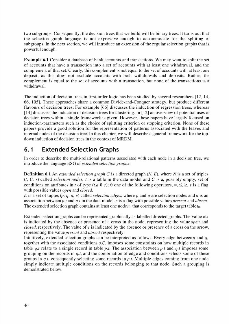
8/8/2019 Knobbe a.J. Multi-Relational Data Mining
http://slidepdf.com/reader/full/knobbe-aj-multi-relational-data-mining 57/129
46
two subgroups. Consequently, the decision trees that we build will be binary trees. It turns out thatthe selection graph language is not expressive enough to accommodate for the splitting of subgroups. In the next section, we will introduce an extension of the regular selection graphs that ispowerful enough.
Example 6.1 Consider a database of bank accounts and transactions. We may want to split the setof accounts that have a transaction into a set of accounts with at least one withdrawal, and thecomplement of that set. Clearly, this complement is not equal to the set of accounts with at least onedeposit, as this does not exclude accounts with both withdrawals and deposits. Rather, thecomplement is equal to the set of accounts with a transaction, but none of the transactions is awithdrawal.
The induction of decision trees in first-order logic has been studied by several researchers [12, 14,66, 105]. These approaches share a common Divide-and-Conquer strategy, but produce differentflavours of decision trees. For example [66] discusses the induction of regression trees, whereas
[14] discusses the induction of decision trees for clustering. In [12] an overview of potential uses of decision trees within a single framework is given. However, these papers have largely focused oninduction-parameters such as the choice of splitting criterion or stopping criterion. None of thesepapers provide a good solution for the representation of patterns associated with the leaves andinternal nodes of the decision tree. In this chapter, we will describe a general framework for the top-down induction of decision trees in the context of MRDM.
([WHQGHG6HOHFWLRQ*UDSKV
In order to describe the multi-relational patterns associated with each node in a decision tree, weintroduce the language ESG of extended selection graphs:
Definition 6.1 An extended selection graph G is a directed graph ( N , E ), where N is a set of triples(t , C, s) called selection nodes, t is a table in the data model and C is a, possibly empty, set of conditions on attributes in t of type (t.a θ c); θ one of the following operators, =, ≤, ≥. s is a flagwith possible values open and closed.
E is a set of tuples ( p, q, a, e) called selection edges, where p and q are selection nodes and a is anassociation between p.t and q.t in the data model. e is a flag with possible values present and absent .The extended selection graph contains at least one node n0 that corresponds to the target table t 0.
Extended selection graphs can be represented graphically as labelled directed graphs. The value of sis indicated by the absence or presence of a cross in the node, representing the value open and
closed , respectively. The value of e is indicated by the absence or presence of a cross on the arrow,representing the value present and absent respectively.Intuitively, extended selection graphs can be interpreted as follows. Every edge between p and q,together with the associated conditions q.C , imposes some constraints on how multiple records intable q.t relate to a single record in table p.t . The association between p.t and q.t imposes somegrouping on the records in q.t , and the combination of edge and conditions selects some of thesegroups in q.t , consequently selecting some records in p.t . Multiple edges coming from one nodesimply indicate multiple conditions on the records belonging to that node. Such a grouping isdemonstrated below.
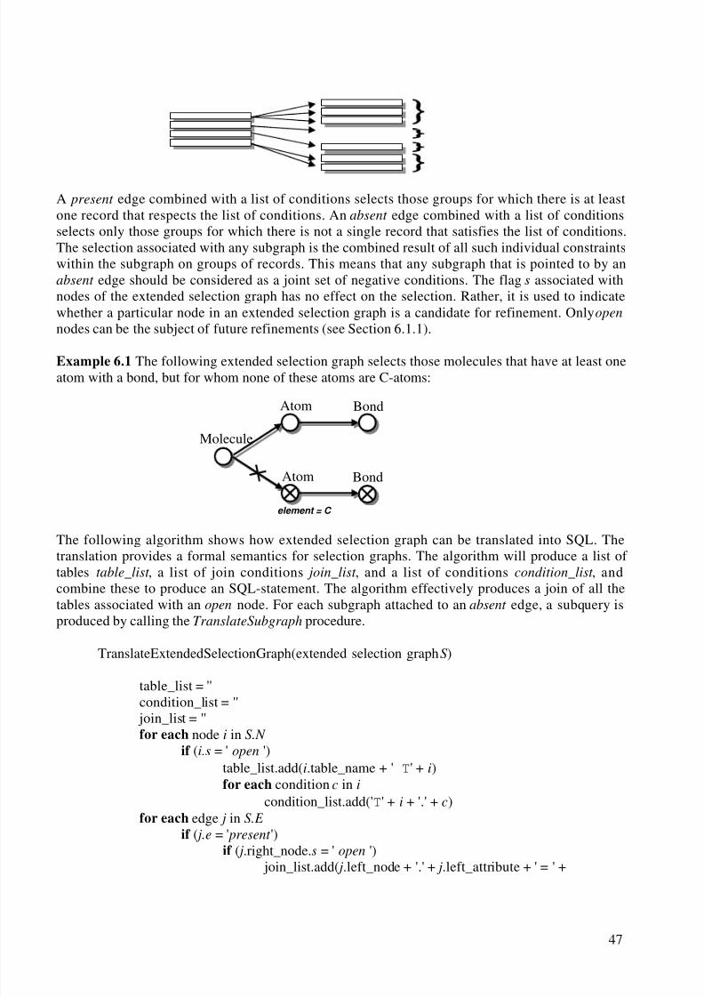
8/8/2019 Knobbe a.J. Multi-Relational Data Mining
http://slidepdf.com/reader/full/knobbe-aj-multi-relational-data-mining 58/129
47
A present edge combined with a list of conditions selects those groups for which there is at leastone record that respects the list of conditions. An absent edge combined with a list of conditionsselects only those groups for which there is not a single record that satisfies the list of conditions.The selection associated with any subgraph is the combined result of all such individual constraintswithin the subgraph on groups of records. This means that any subgraph that is pointed to by anabsent edge should be considered as a joint set of negative conditions. The flag s associated withnodes of the extended selection graph has no effect on the selection. Rather, it is used to indicatewhether a particular node in an extended selection graph is a candidate for refinement. Only open
nodes can be the subject of future refinements (see Section 6.1.1).
Example 6.1 The following extended selection graph selects those molecules that have at least oneatom with a bond, but for whom none of these atoms are C-atoms:
The following algorithm shows how extended selection graph can be translated into SQL. Thetranslation provides a formal semantics for selection graphs. The algorithm will produce a list of tables table_list , a list of join conditions join_list , and a list of conditions condition_list , andcombine these to produce an SQL-statement. The algorithm effectively produces a join of all thetables associated with an open node. For each subgraph attached to an absent edge, a subquery isproduced by calling the TranslateSubgraph procedure.
TranslateExtendedSelectionGraph(extended selection graph S)
table_list = ''
condition_list = '' join_list = ''for each node i in S.N
if (i.s = ' open ')table_list.add(i.table_name + ' T' + i)for each condition c in i
condition_list.add('T' + i + '.' + c)for each edge j in S.E
if ( j.e = ' present ')if ( j.right_node.s = ' open ')
join_list.add( j.left_node + '.' + j.left_attribute + ' = ' +
Atom
Atom Bond
Bond
Molecule
element = C
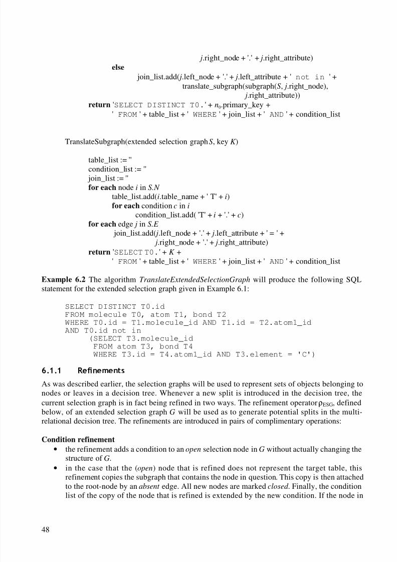
8/8/2019 Knobbe a.J. Multi-Relational Data Mining
http://slidepdf.com/reader/full/knobbe-aj-multi-relational-data-mining 59/129
48
j.right_node + '.' + j.right_attribute)else
join_list.add( j.left_node + '.' + j.left_attribute + ' not in ' +translate_subgraph(subgraph( S, j.right_node),
j.right_attribute))return 'SELECT DISTINCT T0.' + n0.primary_key +
' FROM ' + table_list + ' WHERE ' + join_list + ' AND ' + condition_list
TranslateSubgraph(extended selection graph S, key K )
table_list := ''condition_list := '' join_list := ''for each node i in S.N
table_list.add(i.table_name + ' T' + i)for each condition c in i
condition_list.add( 'T' + i + '.' + c)for each edge j in S.E
join_list.add( j.left_node + '.' + j.left_attribute + ' = ' + j.right_node + '.' + j.right_attribute)
return 'SELECT T0.' + K +
' FROM ' + table_list + ' WHERE ' + join_list + ' AND ' + condition_list
Example 6.2 The algorithm TranslateExtendedSelectionGraph will produce the following SQLstatement for the extended selection graph given in Example 6.1:
SELECT DISTINCT T0.idFROM molecule T0, atom T1, bond T2WHERE T0.id = T1.molecule_id AND T1.id = T2.atom1_idAND T0.id not in
(SELECT T3.molecule_idFROM atom T3, bond T4WHERE T3.id = T4.atom1_id AND T3.element = 'C')
5HILQHPHQWV
As was described earlier, the selection graphs will be used to represent sets of objects belonging to
nodes or leaves in a decision tree. Whenever a new split is introduced in the decision tree, thecurrent selection graph is in fact being refined in two ways. The refinement operator ρESG, definedbelow, of an extended selection graph G will be used as to generate potential splits in the multi-relational decision tree. The refinements are introduced in pairs of complimentary operations:
Condition refinement
• the refinement adds a condition to an open selection node in G without actually changing thestructure of G.
• in the case that the (open) node that is refined does not represent the target table, thisrefinement copies the subgraph that contains the node in question. This copy is then attachedto the root-node by an absent edge. All new nodes are marked closed . Finally, the conditionlist of the copy of the node that is refined is extended by the new condition. If the node in
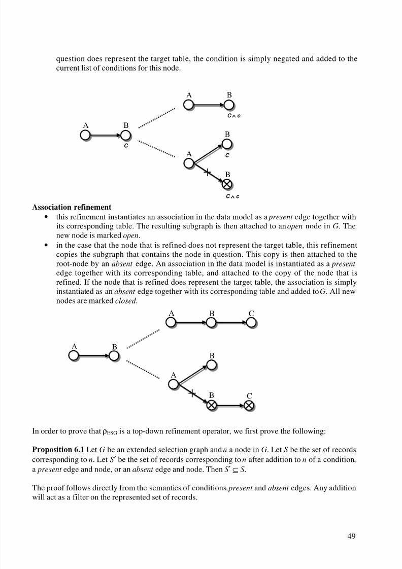
8/8/2019 Knobbe a.J. Multi-Relational Data Mining
http://slidepdf.com/reader/full/knobbe-aj-multi-relational-data-mining 60/129
49
A B
A B C
CB
A
B
A B
C ∧∧∧∧ c
A B
C
B
A
B
C ∧∧∧∧ c
C
question does represent the target table, the condition is simply negated and added to thecurrent list of conditions for this node.
Association refinement
• this refinement instantiates an association in the data model as a present edge together withits corresponding table. The resulting subgraph is then attached to an open node in G. Thenew node is marked open.
• in the case that the node that is refined does not represent the target table, this refinementcopies the subgraph that contains the node in question. This copy is then attached to theroot-node by an absent edge. An association in the data model is instantiated as a present
edge together with its corresponding table, and attached to the copy of the node that isrefined. If the node that is refined does represent the target table, the association is simplyinstantiated as an absent edge together with its corresponding table and added to G. All new
nodes are marked closed .
In order to prove that ρESG is a top-down refinement operator, we first prove the following:
Proposition 6.1 Let G be an extended selection graph and n a node in G. Let S be the set of recordscorresponding to n. Let S′ be the set of records corresponding to n after addition to n of a condition,a present edge and node, or an absent edge and node. Then S′ ⊆ S.
The proof follows directly from the semantics of conditions, present and absent edges. Any addition
will act as a filter on the represented set of records.
8/8/2019 Knobbe a.J. Multi-Relational Data Mining
http://slidepdf.com/reader/full/knobbe-aj-multi-relational-data-mining 61/129
50
Proposition 6.2 Let G be an extended selection graph and n a node in G. Let S and S′ be the set of records corresponding to n before and after a refinement to a node m in the subgraph starting at n,respectively. Then S′ ⊆ S.
Proof Inspection of ρESG shows that all nodes in a subgraph that is attached by an absent edge areclosed , and open otherwise. A path between two open nodes therefore always consists of present
edges. n and m are both open and hence connected by a present path. Now consider two nodes n1
and n2 connected by a present edge, along with two sets of records at n2, S2 and S2′, such that S2′ ⊆S2. We can easily show that for the corresponding sets S1 and S1′ at n1, S1′ ⊆ S1 holds. By inductionwe can now show the same property for any present path between two nodes. Because Proposition6.1 applies to m, we get that S′ ⊆ S.
By applying Proposition 6.2 to the root-node n0 of an extended selection graph that is being refined,
we can see that the refinement in the subgraph works as a filter on the individuals. The possibleabsent subgraph introduced by the two complementary refinements works as an additional filter.Hence:
Proposition 6.3 ρESG is a top-down refinement operator.
0XOWL5HODWLRQDO'HFLVLRQ7UHHV
Top-down induction of decision trees is basically a Divide-and-Conquer algorithm. The algorithmstarts with a single node at the root of the tree, which represents all individuals. By analysing allpossible refinements of the empty extended selection graph, and examining their quality by
applying some interestingness measure, the optimal refinement is determined. This optimalrefinement together with its complement is used to create the patterns associated with the left andthe right branch, respectively. Based on the stopping criterion, it may turn out that the optimalrefinement and its complement do not give cause for further splitting. In this case, a leaf node isintroduced instead. Whenever the optimal refinement does provide a good split, a left and rightbranch are introduced and the procedure is applied to each of these recursively.
BuildTree(tree T , database D, pattern P)
R = OptimalRefinement(P, D)if StoppingCriterion( R)
T = leaf(P)else
Pleft = R(P)Pright = Rcompl(P)BuildTree(left, D, Pleft)BuildTree(right, D, Pright)T = node(left, right, R)
The function OptimalRefinement takes the current pattern P and considers every possible genericpositive refinement with respect to the data model of D. For each of these generic refinements a
multi-relational data mining primitive call is sent to the server that handles the data, and thenecessary statistics are retrieved. The statistics describe the support of all possible refinements
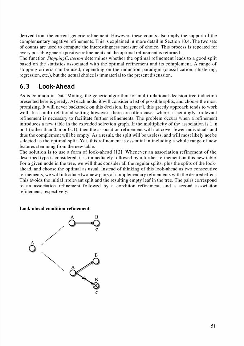
8/8/2019 Knobbe a.J. Multi-Relational Data Mining
http://slidepdf.com/reader/full/knobbe-aj-multi-relational-data-mining 62/129
51
A B
C
A
B
A
B
C
derived from the current generic refinement. However, these counts also imply the support of thecomplementary negative refinements. This is explained in more detail in Section 10.4. The two setsof counts are used to compute the interestingness measure of choice. This process is repeated forevery possible generic positive refinement and the optimal refinement is returned.
The function StoppingCriterion determines whether the optimal refinement leads to a good splitbased on the statistics associated with the optimal refinement and its complement. A range of stopping criteria can be used, depending on the induction paradigm (classification, clustering,regression, etc.), but the actual choice is immaterial to the present discussion.
/RRN$KHDG
As is common in Data Mining, the generic algorithm for multi-relational decision tree inductionpresented here is greedy. At each node, it will consider a list of possible splits, and choose the mostpromising. It will never backtrack on this decision. In general, this greedy approach tends to workwell. In a multi-relational setting however, there are often cases where a seemingly irrelevantrefinement is necessary to facilitate further refinements. The problem occurs when a refinementintroduces a new table in the extended selection graph. If the multiplicity of the association is 1..nor 1 (rather than 0..n or 0..1), then the association refinement will not cover fewer individuals andthus the complement will be empty. As a result, the split will be useless, and will most likely not beselected as the optimal split. Yet, this refinement is essential in including a whole range of newfeatures stemming from the new table.The solution is to use a form of look-ahead [12]. Whenever an association refinement of thedescribed type is considered, it is immediately followed by a further refinement on this new table.For a given node in the tree, we will thus consider all the regular splits, plus the splits of the look-ahead, and choose the optimal as usual. Instead of thinking of this look-ahead as two consecutiverefinements, we will introduce two new pairs of complementary refinements with the desired effect.
This avoids the initial irrelevant split and the resulting empty leaf in the tree. The pairs correspondto an association refinement followed by a condition refinement, and a second associationrefinement, respectively.
Look-ahead condition refinement
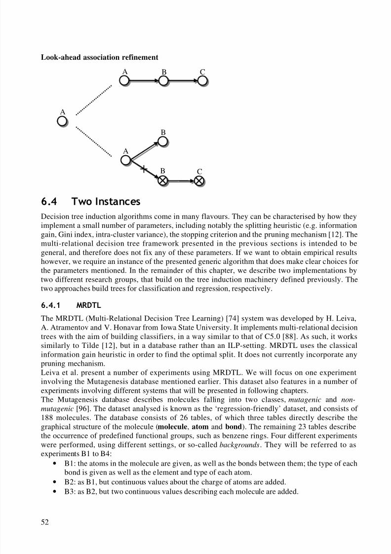
8/8/2019 Knobbe a.J. Multi-Relational Data Mining
http://slidepdf.com/reader/full/knobbe-aj-multi-relational-data-mining 63/129
52
A
A B C
CB
A
B
Look-ahead association refinement
7ZR,QVWDQFHV
Decision tree induction algorithms come in many flavours. They can be characterised by how theyimplement a small number of parameters, including notably the splitting heuristic (e.g. informationgain, Gini index, intra-cluster variance), the stopping criterion and the pruning mechanism [12]. Themulti-relational decision tree framework presented in the previous sections is intended to begeneral, and therefore does not fix any of these parameters. If we want to obtain empirical resultshowever, we require an instance of the presented generic algorithm that does make clear choices forthe parameters mentioned. In the remainder of this chapter, we describe two implementations bytwo different research groups, that build on the tree induction machinery defined previously. The
two approaches build trees for classification and regression, respectively. 05'7/
The MRDTL (Multi-Relational Decision Tree Learning) [74] system was developed by H. Leiva,A. Atramentov and V. Honavar from Iowa State University. It implements multi-relational decisiontrees with the aim of building classifiers, in a way similar to that of C5.0 [88]. As such, it workssimilarly to Tilde [12], but in a database rather than an ILP-setting. MRDTL uses the classicalinformation gain heuristic in order to find the optimal split. It does not currently incorporate anypruning mechanism.Leiva et al. present a number of experiments using MRDTL. We will focus on one experimentinvolving the Mutagenesis database mentioned earlier. This dataset also features in a number of
experiments involving different systems that will be presented in following chapters.The Mutagenesis database describes molecules falling into two classes, mutagenic and non-
mutagenic [96]. The dataset analysed is known as the ‘regression-friendly’ dataset, and consists of 188 molecules. The database consists of 26 tables, of which three tables directly describe thegraphical structure of the molecule (molecule, atom and bond). The remaining 23 tables describethe occurrence of predefined functional groups, such as benzene rings. Four different experimentswere performed, using different settings, or so-called backgrounds. They will be referred to asexperiments B1 to B4:
• B1: the atoms in the molecule are given, as well as the bonds between them; the type of eachbond is given as well as the element and type of each atom.
• B2: as B1, but continuous values about the charge of atoms are added.• B3: as B2, but two continuous values describing each molecule are added.
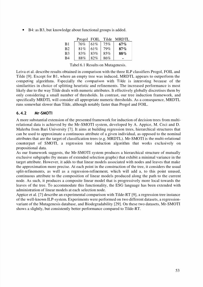
8/8/2019 Knobbe a.J. Multi-Relational Data Mining
http://slidepdf.com/reader/full/knobbe-aj-multi-relational-data-mining 64/129
53
• B4: as B3, but knowledge about functional groups is added.
Progol FOIL Tilde MRDTLB1 76% 61% 75% 67%
B2 81% 61% 79% 87%B3 83% 83% 85% 88%B4 88% 82% 86% -
Tabel 6.1 Results on Mutagenesis.
Leiva et al. describe results obtained in comparison with the three ILP classifiers Progol, FOIL andTilde [9]. Except for B1, where an empty tree was induced, MRDTL appears to outperform thecompeting algorithms. Especially the comparison with Tilde is interesting because of thesimilarities in choice of splitting heuristic and refinements. The increased performance is mostlikely due to the way Tilde deals with numeric attributes. It effectively globally discretises them byonly considering a small number of thresholds. In contrast, our tree induction framework, and
specifically MRDTL will consider all appropriate numeric thresholds. As a consequence, MRDTLruns somewhat slower than Tilde, although notably faster than Progol and FOIL.
0U6027,
A more substantial extension of the presented framework for induction of decision trees from multi-relational data is achieved by the Mr-SMOTI system, developed by A. Appice, M. Ceci and D.Malerba from Bari University [7]. It aims at building regression trees, hierarchical structures thatcan be used to approximate a continuous attribute of a given individual, as opposed to the nominalattributes that are the target of classification trees (e.g. MRDTL). Mr-SMOTI is the multi-relationalcounterpart of SMOTI, a regression tree induction algorithm that works exclusively onpropositional data.As our framework suggests, the Mr-SMOTI system produces a hierarchical structure of mutuallyexclusive subgraphs (by means of extended selection graphs) that exhibit a minimal variance in thetarget attribute. However, it adds to that linear models associated with nodes and leaves that makethe approximation more precise. At each point in the construction of the tree, it considers the usualsplit-refinements, as well as a regression-refinement, which will add a, to this point unused,continuous attribute to the composition of linear models produced along the path to the currentnode. As such, it produces a composite linear model that is progressively more local towards theleaves of the tree. To accommodate this functionality, the ESG language has been extended withadministration of linear models at each selection node.Appice et al. [7] describe an experimental comparison with Tilde-RT [9], a regression tree instance
of the well-known ILP-system. Experiments were performed on two different datasets, a regression-variant of the Mutagenesis database, and Biodegradability [29]. On these two datasets, Mr-SMOTIshows a slightly, but consistently better performance compared to Tilde-RT.

8/8/2019 Knobbe a.J. Multi-Relational Data Mining
http://slidepdf.com/reader/full/knobbe-aj-multi-relational-data-mining 65/129
This page intentionally left blank
8/8/2019 Knobbe a.J. Multi-Relational Data Mining
http://slidepdf.com/reader/full/knobbe-aj-multi-relational-data-mining 66/129
55
$JJUHJDWH)XQFWLRQV
As was outlined in Chapter 4, we can identify two important approaches to capturing localstructure. The first approach describes groups of records by means of existential features. Thesecond approach focuses on features of the group as a whole, by means of aggregate functions. TheMRDM technology presented so far has been based on capturing local structure exclusively throughexistential features. In this and the following two chapters, we investigate the extra benefits thataggregate functions have to offer. The present chapter describes the basic properties of aggregatefunctions, and how a good set of features can be selected from the potentially infinite set of aggregate functions. Having a set of well-chosen aggregate functions will allow us to describe theessence of the structural information over a wide variety of structures.
$JJUHJDWH)XQFWLRQV
We define an aggregate function as a function that takes as input a set of records in a database,related through the associations in the data model, and produces a single value as output. Aggregatefunctions will be used to project information stored in several tables on one of these tables,
essentially adding virtual attributes to this table. In the case where the information is projected onthe target table, and structural information belonging to an individual is summarised as a newfeature of that individual, aggregate functions can be thought of as a form of feature construction.The broad definition used here includes aggregate functions of a great variety of complexity. Animportant aspect of the complexity of an aggregate function is the number of (associations between)tables it involves. As each aggregate function essentially considers a subset of the data model, wecan use our three previously defined complexity-measures for data models to characterise aggregatefunctions. Specifically association-depth is useful to classify aggregate functions. An aggregatefunction of association-depth 0 involves just one table, and is hence, a case of propositional featureconstruction. In their basic usage, aggregate functions found in SQL (count, min, sum, etc.) have anassociation-depth of 1, whereas association-deeper aggregate functions represent some form of
8/8/2019 Knobbe a.J. Multi-Relational Data Mining
http://slidepdf.com/reader/full/knobbe-aj-multi-relational-data-mining 67/129
56
multi-relational pattern (benzene-rings in molecules, etc.). Using this classification of association-depth, we give some examples to illustrate the range of possibilities.
da( A) = 0:
• Propositions (adult = (age 18))• Arithmetic functions (area = (width · length))
da( A) = 1:• Count, count with condition• Count distinct• Min, max, sum, avg• Exists, exists with condition• Select record (eldest son, first contract)• Mode
da( A) > 1:• Exists substructure• Count substructure• Conjunction of aggregate functions (maximum count of children)
Clearly the list of possible classes of aggregate functions is long, and the number of instances isinfinite. An overview of interesting classes of aggregate functions, along with a hierarchy of increasing complexity is given in [85]. In order to arrive at a practical and manageable set of aggregate functions, we will have to drastically limit the range of classes and instances. Apart fromdeterministic and heuristic rules to select good candidates, pragmatic limitations to a small set of
aggregate function classes are unavoidable. In this thesis, we have chosen to restrict ourselves to theclasses available in SQL and combinations thereof.
$JJUHJDWLRQ
Let us consider two tables P and Q, neither of which needs to be the target table, that are joined byan association A. By aggregating over A, information can be added to P about the structuralproperties of A, as well as the data within Q. To aggregate Q, a set of aggregate functions of association-depth 1 is needed.As was demonstrated before, the multiplicity of association A influences the search space of multi-relational patterns involving A. The same is true for aggregation over A using aggregate functions.The choice of aggregate functions depends on the multiplicity of A. In particular, if we aggregate Q
over A, only the multiplicity on the side of Q is relevant. This is because an association generallydescribes two relationships between the records in both tables, one for each direction. The followingfour options exist:1 For every record in P there is but a single record in Q. This is basically a look-up over a
foreign key relation, and no aggregate functions are required. A simple join will add all non-key attributes of Q to P.
0..1 Similar to the 1 case, but now a look-up may fail because a record in P may not have acorresponding record in Q. An outer join is necessary, which fills in NULL values formissing records.
1..n For every record in P, there is at least one record in Q. Aggregate functions are required in
order to capture the information in the group of records belonging to a single record in P.
8/8/2019 Knobbe a.J. Multi-Relational Data Mining
http://slidepdf.com/reader/full/knobbe-aj-multi-relational-data-mining 68/129
57
0..n Similar to the 1..n case, but now the value of certain aggregate functions may be undefineddue to empty groups. Special care will need to be taken to deal with the resulting NULLvalues.
Let us now consider the 1..n case in more detail. A imposes a grouping on the records in Q. For m
records in P there will be m groups of records in Q. Because of the set-semantics of relationaldatabases every group can be described by a collection of histograms or data-cubes. We can nowview an aggregate function instance as a function of one of these types of histograms. For examplethe mode aggregate function for an attribute Q.a simply returns the value corresponding to thehighest count in the histogram of Q.a. Note that m groups will produce m histograms andconsequently m values for one aggregate function instance, one for each record in P. The notion of functions of histograms helps us to define relevant aggregate function classes.
count The count aggregate function is the most obvious aggregate function through its directrelation to histograms. The most basic instance without conditions simply returns the single value inthe 0-dimensional histogram. Adding a single condition requires a 1-dimensional histogram of the
attribute involved in the condition. For example, the number of sons in a family can be computedfrom a histogram of gender of that family. An attribute with a cardinality c will produce c aggregatefunction instances of count with one condition.There is some overlap in the patterns that can be expressed using the count aggregate function andthose expressed by existential features. Testing for a count greater than zero obviously correspondsto existence. Testing for a count greater than some threshold t however, requires a refinement-depthof O(t
2) in existential features, as a quadratic number of inequalities needs to be added in order toguarantee correct counting. Things become even worse for existential features when the < operatoris used, as it requires the use of negation in a way that (extended) selection graphs (as well as thelanguage bias of many ILP algorithms) does not cater to. The use of the count aggregate function isclearly more powerful in these respects.
min and max The two obvious aggregate functions for numeric attributes, min and max, exhibitsimilar behaviour. Again there is a trivial way of computing min and max from the histogram; thesmallest and largest values having a non-zero count, respectively. The min and max aggregatefunctions support another type of constraint commonly used in existential feature-based algorithms,exists with a numeric constraint. Lemma 4.1 describes the correspondence between the minimumand maximum of a group of numbers, and the occurrence of particular values in the group. It simplystates that testing whether the maximum is greater than some threshold is equivalent to testingwhether any value is greater than t . Analogous for min. It is important to note the combination of max and ≥, and min and ≤. If max were to be used in combination with ≤ or =, then the existentialfeature equivalent would again require the use of negation.
Such use of the min and max aggregate function gives us a natural means of introducing theuniversal quantor ∀: all values are required to be above the minimum, or below the maximum.Another advantage of the min and max aggregate function is that they each replace a set of binaryexists aggregate function instances (one for each threshold), making the representation of virtualattributes a lot more compact. The following lemma illustrates how the min and max function caneasily capture local structure in a way that would require undesirable universal quantification (ornegation) otherwise.
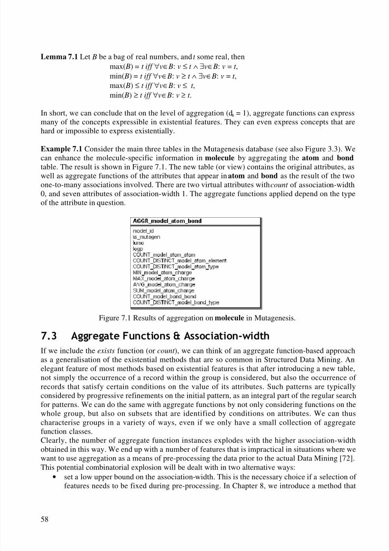
8/8/2019 Knobbe a.J. Multi-Relational Data Mining
http://slidepdf.com/reader/full/knobbe-aj-multi-relational-data-mining 69/129
58
Lemma 7.1 Let B be a bag of real numbers, and t some real, thenmax( B) = t iff ∀v∈ B: v ≤ t ∧ ∃v∈ B: v = t ,min( B) = t iff ∀v∈ B: v ≥ t ∧ ∃v∈ B: v = t ,max( B) ≤ t iff ∀v∈ B: v ≤ t ,
min( B) ≥ t iff ∀v∈ B: v ≥ t .
In short, we can conclude that on the level of aggregation (da = 1), aggregate functions can expressmany of the concepts expressible in existential features. They can even express concepts that arehard or impossible to express existentially.
Example 7.1 Consider the main three tables in the Mutagenesis database (see also Figure 3.3). Wecan enhance the molecule-specific information in molecule by aggregating the atom and bond
table. The result is shown in Figure 7.1. The new table (or view) contains the original attributes, aswell as aggregate functions of the attributes that appear in atom and bond as the result of the twoone-to-many associations involved. There are two virtual attributes with count of association-width
0, and seven attributes of association-width 1. The aggregate functions applied depend on the typeof the attribute in question.
Figure 7.1 Results of aggregation on molecule in Mutagenesis.
$JJUHJDWH)XQFWLRQV$VVRFLDWLRQZLGWK
If we include the exists function (or count ), we can think of an aggregate function-based approachas a generalisation of the existential methods that are so common in Structured Data Mining. Anelegant feature of most methods based on existential features is that after introducing a new table,not simply the occurrence of a record within the group is considered, but also the occurrence of
records that satisfy certain conditions on the value of its attributes. Such patterns are typicallyconsidered by progressive refinements on the initial pattern, as an integral part of the regular searchfor patterns. We can do the same with aggregate functions by not only considering functions on thewhole group, but also on subsets that are identified by conditions on attributes. We can thuscharacterise groups in a variety of ways, even if we only have a small collection of aggregatefunction classes.Clearly, the number of aggregate function instances explodes with the higher association-widthobtained in this way. We end up with a number of features that is impractical in situations where wewant to use aggregation as a means of pre-processing the data prior to the actual Data Mining [72].This potential combinatorial explosion will be dealt with in two alternative ways:
• set a low upper bound on the association-width. This is the necessary choice if a selection of features needs to be fixed during pre-processing. In Chapter 8, we introduce a method that
8/8/2019 Knobbe a.J. Multi-Relational Data Mining
http://slidepdf.com/reader/full/knobbe-aj-multi-relational-data-mining 70/129
59
repeatedly flattens pairs of tables by aggregation to arrive at a single target table containinga range of multi-relational features, a process known as propositionalisation. For thismethod we restrict ourselves to the aggregate function classes available in SQL, and fix wa
1: for count we add up to one condition on a nominal attribute (no numeric conditions), and
for the remaining classes no conditions as they already have an association-width of 1.• allow any association-width, but only through progressive refinement. This approach onlyworks if patterns with aggregate functions are considered dynamically, rather than prior toData Mining. In Chapter 9, we examine an upgrade of the rule discovery algorithmpresented in Chapter 5 that works along these lines.
If we want to consider aggregate functions of higher association-width by progressively refining theset of records that is aggregated, we will need to examine how the value of the aggregate functionsdepends on different sets of records. The following observations will be relevant for selectingproper refinements (see Section 9.3).
Definition 7.1
1. An aggregate function f is ascending iff , given sets of records S and S', S' ⊆ S f (S' ) f (S).
2. An aggregate function f is descending iff , given sets of records S and S' , S' ⊆ S f (S' ) f (S).
Lemma 7.21. Aggregate functions count , count distinct and max are ascending.2. Aggregate function min is descending.3. Aggregate functions sum and avg are neither ascending nor descending.
Example 7.2 In the Mutagenesis problem database [95], there are tables for the concepts molecule,atom and bond. Some promising aggregate functions to describe the relation between molecule andatom are:
count(atom), min(atom.charge), avg(atom.charge)
We might also have similar functions for C-atoms in a molecule, or for C-atoms involved in adouble bond. Clearly, the count decreases if we only consider a subset of atoms, such as the C-atoms. In contrast, the minimum charge will increase.

8/8/2019 Knobbe a.J. Multi-Relational Data Mining
http://slidepdf.com/reader/full/knobbe-aj-multi-relational-data-mining 71/129
This page intentionally left blank
8/8/2019 Knobbe a.J. Multi-Relational Data Mining
http://slidepdf.com/reader/full/knobbe-aj-multi-relational-data-mining 72/129
61
$JJUHJDWH)XQFWLRQV3URSRVLWLRQDOLVDWLRQ
In this chapter we will consider an approach to analysing multi-relational data that is different fromthe remainder of MRDM algorithms presented in this thesis. Rather than searching through a searchspace of multi-relational patterns and progressively discovering more complex structures, we willbe using traditional propositional techniques. In order to apply these techniques with at least somedegree of success, it will be necessary to transfer the original multi-table database into a singletable, with one record for each individual. In order not to ignore the information in the tables otherthan the target table, the transformed table will contain an (often large) collection of features thatcapture different aspects of the structure in the individuals. This process of transforming a multi-relational database into a single table is known as propositionalisation.The idea of propositionalisation (the construction of one table) is not new. Several relativelysuccessful algorithms have been proposed in the context of Inductive Logic Programming (ILP) [6,24, 65, 67, 97]. A common aspect of these algorithms is that the derived table consists solely of
binary features, each corresponding to a (promising) clause discovered by an ILP-algorithm. Thischapter however presents an alternative approach, based on the aggregate function machineryintroduced in Chapter 7. It does not involve searching for relevant substructure, but rather relies onrepeatedly summarising pairs of tables into a single new table by means of aggregate functions.It may seem that having to select a fixed set of features before actually mining the data gives ourapproach a disadvantage compared to the more dynamic nature of regular MRDM algorithms. Wewill show, among others with experiments, that the propositionalisation approach has alternativebenefits that allow it to compete with these algorithms. Their good performance can not only beattributed to how the transformation interacts with subsequent mining, but to a greater extent to therich features that can be extracted from individuals by using aggregate functions.
8/8/2019 Knobbe a.J. Multi-Relational Data Mining
http://slidepdf.com/reader/full/knobbe-aj-multi-relational-data-mining 73/129
62
3URSRVLWLRQDOLVDWLRQ
In this section we describe the basic concepts involved in propositionalisation, and provide somedefinitions. We define propositionalisation as the process of transforming a multi-relational datasetinto a propositional dataset with derived attribute-value features, describing specific structuralproperties of the individuals. The process can thus be thought of as summarising data stored inmultiple tables in a single table (the target table) containing one record per individual. The aim of this process, of course, is to pre-process multi-relational data for subsequent analysis by attribute-value learners.We will be using this definition in the broadest sense. We will make no assumptions about the datatype of the derived attribute (binary, nominal, numeric, etc.) nor do we specify what language willbe used to specify the propositional features.Traditionally, propositionalisation has been approached from an ILP standpoint with only binaryfeatures, expressed in first-order logic [6, 24, 67, 65]. To our knowledge, the use of other aggregatefunctions than existence has been limited. One example is given in [29], which describes a
propositionalisation-step where numeric attributes were defined for counts of differentsubstructures. Friedman et al. [38] also mention aggregate functions as a means of establishingprobabilistic relationships between objects in pairs of tables. It is our aim to analyse theapplicability of a broader range of aggregate functions.With a growing availability of algorithms from the fields of ILP and MRDM, one might wonderwhy such a cumbersome pre-processing step is desirable in the first place, instead of applying oneof these algorithms to the multi-relational data directly. The following is a (possibly incomplete) listof reasons:
• Pragmatic choice for specific propositional techniques. People may wish to apply theirfavourite attribute-value learner, or only have access to commercial of-the-shelf DataMining tools. Good examples can be found in the contributions to the Financial dataset
challenge at PKDD conferences [106].• Superiority of propositional algorithms with respect to certain Machine Learningparameters. Although extra facilities are quickly being added to existing Structured DataMining engines, propositional algorithms still have a head start concerning handling of numeric values, regression, distance measures, cumulativity etc.
• Greater speed of propositional algorithms. This advantage of course only holds if thepreceding work for propositionalisation was limited, or performed only once and thenreused during multiple attribute-value learning sessions.
• Advantages related to multiple consecutive learning steps. Because two learning steps areapplied, we are effectively combining two search strategies. The first step essentiallytransforms a multi-relational search space into a propositional one. The second step thenuses these complex patterns to search deeper than either step could achieve when applied inisolation. This issue is investigated in more detail in the remainder of this section.
The term propositionalisation leads to some confusion because, although it pertains to the initialstep of flattening a multi-relational database, it is often used to indicate the whole approach,including the subsequent propositional learning step. Because we are mostly interested in the twosteps in unison, and for the sake of discussion, we introduce the following generic algorithm. Thename is taken from Czech, and describes a two-step dance.
Polka (database D, data model M , integer r , p)
P= MRDM (
D,
M ,
r ) R = PDM (P, p)
8/8/2019 Knobbe a.J. Multi-Relational Data Mining
http://slidepdf.com/reader/full/knobbe-aj-multi-relational-data-mining 74/129
63
The algorithm takes a database D and data model M (acting as declarative bias), and first applies aMulti-Relational Data Mining algorithm MRDM. The resulting propositional features P are then fedto a propositional Data Mining algorithm PDM, producing result R. We use the integers r and p
very informally to identify the extent of the multi-relational and propositional search, respectively.
Note that the propositionalisation step is independent of subsequent use in propositional learning.In order to characterise the extent of the search more formally, we consider the complexitymeasures for the most complex patterns in the search space. We can thus characterise bothindividual patterns, as well as algorithms.
Lemma 8.11. da(Polka) = da(MRDM)2. dr(Polka) = dr(MRDM) · dr(PDM)3. wa(Polka) = wa(MRDM)
Not surprisingly, the complexity of Polka depends largely on the complexity of the actual
propositionalisation step. However, Lemma 8.1 2. demonstrates that Polka considers veryrefinement-deep patterns, in fact deeper than a multi-relational algorithm would consider inisolation. This is due to the combining of search spaces mentioned earlier. Later on we will examinethe search restrictions that the use of aggregate functions have on the propositionalisation step andthus on Polka.
7KH5ROO8S$OJRULWKP
With the foundations provided in the previous sections we can now define a basicpropositionalisation algorithm. The algorithm will traverse the data model graph and repeatedly usethe aggregation operation to project data from one table onto another, until all information has beenaggregated at the target table. Although this repeated summarisation can be done in several ways,we will describe a basic algorithm, called RollUp.The RollUp algorithm performs a depth-first search (DFS) through the data model, up to a specifieddepth. Whenever the recursive algorithm reaches its maximum depth or a leaf in the graph, it will“roll up” the relevant table by aggregating it onto the parent in the DFS tree. Internal nodes in thetree will again be aggregated after all its children have been aggregated. This means that attributesconsidered deep in the tree may be aggregated multiple times. The process continues until all tablesare summarised onto the target table. Combined with a propositional learner we obtain an instanceof Polka. The following pseudo code describes RollUp more formally:
RollUp (table T , data model M , integer d )
V = T
if d > 0for all associations A from T in M
W = RollUp(T .getTable( A), M , d -1)S = Aggregate(W , A)V .add(S)
return V
The effect of RollUp is that each attribute appearing in a table other than the target table will appear
several times in aggregated form in the resulting view. This multiple occurrence happens for two
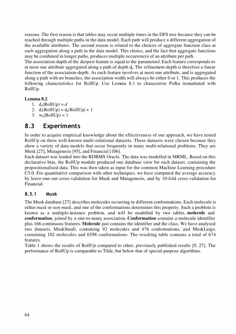
8/8/2019 Knobbe a.J. Multi-Relational Data Mining
http://slidepdf.com/reader/full/knobbe-aj-multi-relational-data-mining 75/129
64
reasons. The first reason is that tables may occur multiple times in the DFS tree because they can bereached through multiple paths in the data model. Each path will produce a different aggregation of the available attributes. The second reason is related to the choices of aggregate function class ateach aggregation along a path in the data model. This choice, and the fact that aggregate functions
may be combined in longer paths, produces multiple occurrences of an attribute per path.The association-depth of the deepest feature is equal to the parameter d . Each feature corresponds toat most one attribute aggregated along a path of depth da. The refinement-depth is therefore a linearfunction of the association-depth. As each feature involves at most one attribute, and is aggregatedalong a path with no branches, the association-width will always be either 0 or 1. This produces thefollowing characteristics for RollUp. Use Lemma 8.1 to characterise Polka instantiated withRollUp.
Lemma 8.2
1. da(RollUp) = d
2. dr(RollUp) = da(RollUp) + 1
3. wa(RollUp) = 1
([SHULPHQWV
In order to acquire empirical knowledge about the effectiveness of our approach, we have testedRollUp on three well-known multi-relational datasets. These datasets were chosen because theyshow a variety of data models that occur frequently in many multi-relational problems. They areMusk [27], Mutagenesis [95], and Financial [106].Each dataset was loaded into the RDBMS Oracle. The data was modelled in MRML. Based on thisdeclarative bias, the RollUp module produced one database view for each dataset, containing thepropositionalised data. This was then taken as input for the common Machine Learning procedureC5.0. For quantitative comparison with other techniques, we have computed the average accuracyby leave-one-out cross-validation for Musk and Mutagenesis, and by 10-fold cross-validation forFinancial.
0XVN
The Musk database [27] describes molecules occurring in different conformations. Each molecule iseither musk or non-musk , and one of the conformations determines this property. Such a problem isknown as a multiple-instance problem, and will be modelled by two tables, molecule andconformation, joined by a one-to-many association. Conformation contains a molecule identifierplus 166 continuous features. Molecule just contains the identifier and the class. We have analysedtwo datasets, MuskSmall, containing 92 molecules and 476 conformations, and MuskLarge,
containing 102 molecules and 6598 conformations. The resulting table contains a total of 674features.Table 1 shows the results of RollUp compared to other, previously published results [9, 27]. Theperformance of RollUp is comparable to Tilde, but below that of special-purpose algorithms.
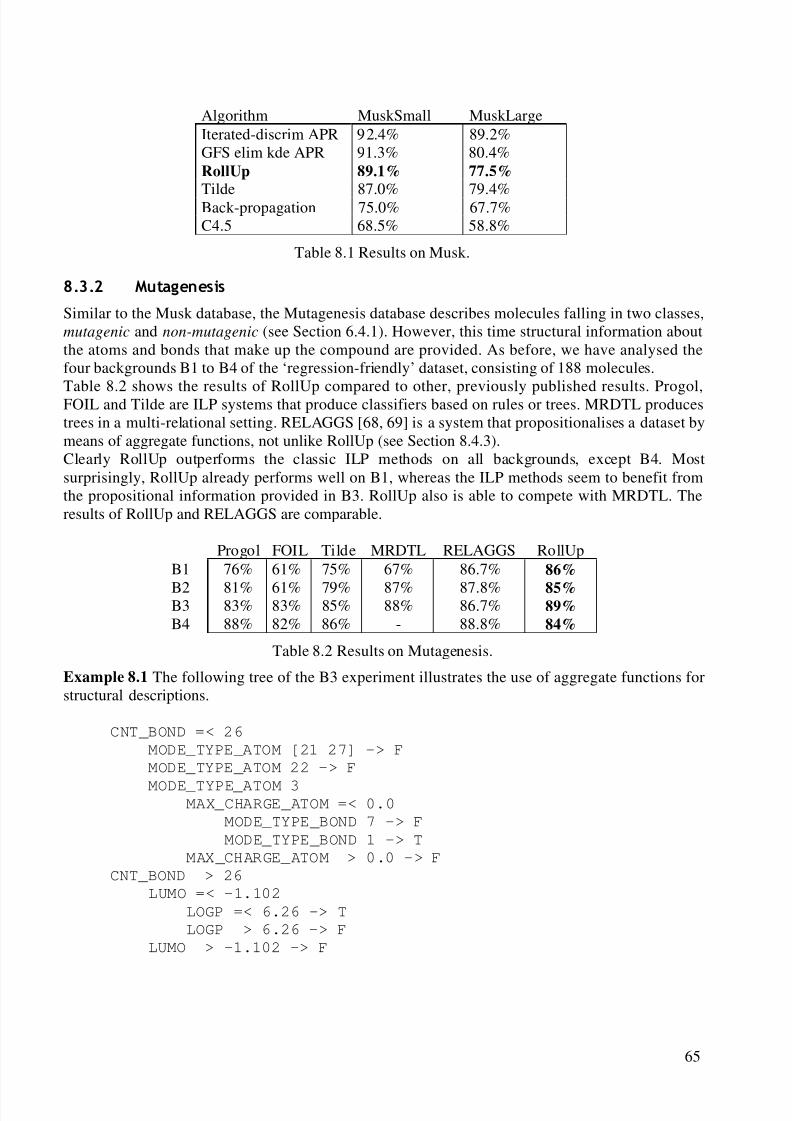
8/8/2019 Knobbe a.J. Multi-Relational Data Mining
http://slidepdf.com/reader/full/knobbe-aj-multi-relational-data-mining 76/129
65
Algorithm MuskSmall MuskLargeIterated-discrim APR 92.4% 89.2%GFS elim kde APR 91.3% 80.4%RollUp 89.1% 77.5%
Tilde 87.0% 79.4%Back-propagation 75.0% 67.7%C4.5 68.5% 58.8%
Table 8.1 Results on Musk.
0XWDJHQHVLV
Similar to the Musk database, the Mutagenesis database describes molecules falling in two classes,mutagenic and non-mutagenic (see Section 6.4.1). However, this time structural information aboutthe atoms and bonds that make up the compound are provided. As before, we have analysed thefour backgrounds B1 to B4 of the ‘regression-friendly’ dataset, consisting of 188 molecules.
Table 8.2 shows the results of RollUp compared to other, previously published results. Progol,FOIL and Tilde are ILP systems that produce classifiers based on rules or trees. MRDTL producestrees in a multi-relational setting. RELAGGS [68, 69] is a system that propositionalises a dataset bymeans of aggregate functions, not unlike RollUp (see Section 8.4.3).Clearly RollUp outperforms the classic ILP methods on all backgrounds, except B4. Mostsurprisingly, RollUp already performs well on B1, whereas the ILP methods seem to benefit fromthe propositional information provided in B3. RollUp also is able to compete with MRDTL. Theresults of RollUp and RELAGGS are comparable.
Progol FOIL Tilde MRDTL RELAGGS RollUpB1 76% 61% 75% 67% 86.7% 86%
B2 81% 61% 79% 87% 87.8% 85%B3 83% 83% 85% 88% 86.7% 89%B4 88% 82% 86% - 88.8% 84%
Table 8.2 Results on Mutagenesis.
Example 8.1 The following tree of the B3 experiment illustrates the use of aggregate functions forstructural descriptions.
CNT_BOND =< 26
MODE_TYPE_ATOM [21 27] -> F
MODE_TYPE_ATOM 22 -> F
MODE_TYPE_ATOM 3MAX_CHARGE_ATOM =< 0.0
MODE_TYPE_BOND 7 -> F
MODE_TYPE_BOND 1 -> T
MAX_CHARGE_ATOM > 0.0 -> F
CNT_BOND > 26
LUMO =< -1.102
LOGP =< 6.26 -> T
LOGP > 6.26 -> F
LUMO > -1.102 -> F
8/8/2019 Knobbe a.J. Multi-Relational Data Mining
http://slidepdf.com/reader/full/knobbe-aj-multi-relational-data-mining 77/129
66
)LQDQFLDO
The third experiment covers the Financial database as described in Section 5.3. A near perfect scoreof 99.9% was achieved on this dataset. Due to the great variety of problem definitions described inthe literature, quantitative comparisons with previous results are impossible. Similar (descriptive)
analyses of loan-quality however, have never produced the pattern responsible for RollUp’s goodperformance. The aggregation approach proved particularly successful on the large transaction
table (1056320 records). This table has sometimes been left out of other experiments due toscalability problems.
'LVFXVVLRQ
The experimental results in the previous section demonstrate that our approach is at leastcompetitive with existing techniques based on existential features, such as Progol, Tilde, andMRDTL. Our approach has two major differences with these techniques, which may be the sourceof the good performance: the use of aggregate functions and the use of propositionalisation. Let us
consider the contribution of each of these in turn.
$JJUHJDWHIXQFWLRQV
There is an essential difference in the way a group of records is characterised by existential featuresand by aggregate functions. Existential features are based on the occurrence of one or more recordsin the group with certain properties. Aggregate functions on the other hand typically describe thegroup as a whole: each record has some influence on the value of the aggregate function. The resultof this difference is that existential features and aggregate functions provide two unique feature-spaces to the learning procedure. Each feature-space has its advantages and disadvantages, and maybe more or less suitable for the problem at hand.Although the feature-spaces produced by existential features and aggregate functions have entirelydifferent characteristics, there is still some overlap. As was shown in Chapter 7, some aggregatefunctions are very similar in behaviour to existential features. The common features in the twospaces typically
• select one or a few records in a group (min and <, max and >, count > 0 for some condition).• involve a single attribute: wa ≤ 1• have a relatively low association-depth.
If these properties hold, aggregate-based learning procedures will generally perform better, as theycan dispose of the common selective aggregate functions, as well as the complete aggregatefunctions such as sum and avg.Data models with a low association-depth are quite common in database design, and are called star-
shaped (da = 1) or snowflake schemata (da > 1). The Musk dataset is the most simple example of astar-shaped model. The data model of Mutagenesis consists for the large part of a star-shapedmodel, and Financial is essentially a snowflake schema. Many real-world datasets described in theliterature as SDM applications essentially have such a manageable structure. Moreover, results onthese datasets frequently exhibit the extra condition of wa ≤ 1. Some illustrative examples are givenin [29, 95].
3URSRVLWLRQDOLVDWLRQ
According to lemma 8.2, Polka has the ability to discovery patterns that have a bigger refinement-depth than either of its steps has. This is demonstrated by the experiments with the particularinstance of Polka presented here. RollUp produces relatively association-deep, and thus,refinement-deep features. These refinement-deep features are combined in the decision tree. Some
8/8/2019 Knobbe a.J. Multi-Relational Data Mining
http://slidepdf.com/reader/full/knobbe-aj-multi-relational-data-mining 78/129
67
leaves represent very refinement-deep patterns, even though their support is still sufficient. This isan advantage of Polka (propositionalisation + propositional learning) over SDM algorithms ingeneral.Next to advantages related to expressiveness, there are more practical reasons for using Polka. Once
the propositionalisation stage is finished, a large part of the computationally expensive work isdone, and the derived view can be analysed multiple times. This not only provides a greaterefficiency, but also gives the analyst more flexibility in choosing the right modelling techniquefrom a large range of well-developed commercially available set of tools. The analyst can vary thestyle of analysis (trees, rules, neural, instance-based) as well as the Data Mining task (classification,regression).
5HODWHG:RUN
Two alternative MRDM approaches implement propositionalisation by means of aggregatefunctions. The RELAGGS system [68, 69] uses a slightly larger collection of aggregate functionclasses to summarise groups of records. The essential difference with RollUp however, is where
aggregation is applied. Rather than recursively joining and aggregating pairs of tables towards thetarget table, RELAGGS propagates the key of the individual to each table, effectively turning thedata model into a star schema (association-depth 1). It then applies aggregate functions to all tables,as if directly connected to the target table. This process produces the same result (given the samecollection of aggregate function classes) whenever a database of association-depth 1 or less isprocessed. On association-deeper data models however, RollUp will nest aggregate functions (e.g.average of the count), whereas RELAGGS will aggregate over the transitive association.Perlich et al. [85] describe another approach that treats the data model as a star schema, althoughnot using propagated keys, but aggregate functions over the joins along paths in the data modelstarting from the target table. This work focuses on concept classes of aggregate functions that gobeyond the basic functions employed by RollUp and RELAGGS. Experimental results show theclear benefit of using more elaborate aggregate functions. To some degree, these more complexfunctions correspond to the resulting nested functions of RollUp, or constructs described in Chapter9.A comparison between RELAGGS and two propositionalisation approaches based on binaryfeatures produced by ILP algorithms is presented in [69]. The results are not conclusive in favour of either approach, but aggregate functions appear to work better in domains where counting anddealing with numbers is relevant. Binary features are preferred in domains were the occurrence of association-deep and association-wide structures is of significance. This coincides with ourfindings.

8/8/2019 Knobbe a.J. Multi-Relational Data Mining
http://slidepdf.com/reader/full/knobbe-aj-multi-relational-data-mining 79/129
This page intentionally left blank
8/8/2019 Knobbe a.J. Multi-Relational Data Mining
http://slidepdf.com/reader/full/knobbe-aj-multi-relational-data-mining 80/129
69
$JJUHJDWH)XQFWLRQV5XOH'LVFRYHU\
The experiments in the previous chapter demonstrate the power of aggregate functions. Particularlyon databases that combine a high level of non-determinacy with large numbers of (numeric)attributes, these aggregate functions are a promising means of capturing local structure.Unfortunately, the propositionalisation method in which we embedded these functions has adisadvantage that reduces their potential. This has to do with the static nature of the featuresproduced in the propositionalisation step. The small set of aggregate functions employed produces amoderate set of fixed features which cannot be modified when the actual mining takes place.In contrast, the top-down algorithms presented in Chapters 5 and 6 select a new set of relevantfeatures dynamically, based on the subgroup under investigation, say at a branch in a decision tree.As such, the range of substructures that can be recognised is not fixed from the outset. In thischapter we propose a method that combines the expressive power of aggregate functions with thedesired dynamic behaviour of the top-down algorithms.The aim is to include aggregate functions in the Rule Discovery framework introduced in Chapter 5.The selection graphs pattern language is extended to deal with our need for aggregation. Edges in
the graph, which originally represented existential constraints, are annotated with aggregatefunctions that summarise the substructure selected by the connected subgraph. Although wecontinue to use the restricted set of aggregate functions, a large range of features can be consideredby refining the subgraph with the usual conditions, and even with further aggregation-basedconditions on the subgraph.The overall structure of the Rule Discovery method remains unchanged. The primary changes dealwith the richer pattern language and the refinement operator that introduces aggregate functions intoa given pattern. We will show that extra care needs to be taken in order to guarantee that therefinement operator is actually a specialisation operator. Catering to aggregation also requires morecomplex data mining primitives. This subject is covered in Section 10.5.Related work on aggregate functions primarily focuses on propositionalisation [59, 68, 69, 85]. To
our knowledge, only a single method (relational probability trees [84]) introduces aggregate
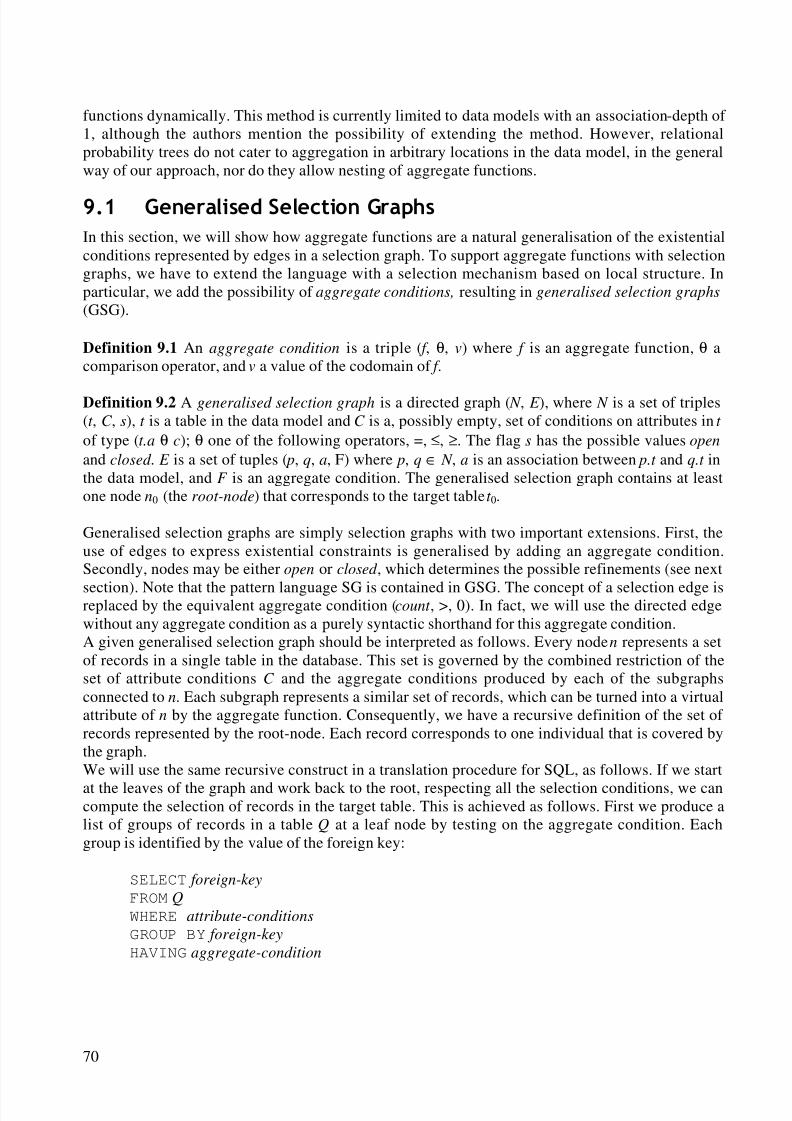
8/8/2019 Knobbe a.J. Multi-Relational Data Mining
http://slidepdf.com/reader/full/knobbe-aj-multi-relational-data-mining 81/129
70
functions dynamically. This method is currently limited to data models with an association-depth of 1, although the authors mention the possibility of extending the method. However, relationalprobability trees do not cater to aggregation in arbitrary locations in the data model, in the generalway of our approach, nor do they allow nesting of aggregate functions.
*HQHUDOLVHG6HOHFWLRQ*UDSKV
In this section, we will show how aggregate functions are a natural generalisation of the existentialconditions represented by edges in a selection graph. To support aggregate functions with selectiongraphs, we have to extend the language with a selection mechanism based on local structure. Inparticular, we add the possibility of aggregate conditions, resulting in generalised selection graphs
(GSG).
Definition 9.1 An aggregate condition is a triple ( f , θ, v) where f is an aggregate function, θ acomparison operator, and v a value of the codomain of f .
Definition 9.2 A generalised selection graph is a directed graph ( N , E ), where N is a set of triples(t , C , s), t is a table in the data model and C is a, possibly empty, set of conditions on attributes in t
of type (t.a θ c); θ one of the following operators, =, ≤, ≥. The flag s has the possible values open
and closed . E is a set of tuples ( p, q, a, F) where p, q ∈ N , a is an association between p.t and q.t inthe data model, and F is an aggregate condition. The generalised selection graph contains at leastone node n0(the root-node) that corresponds to the target table t 0.
Generalised selection graphs are simply selection graphs with two important extensions. First, theuse of edges to express existential constraints is generalised by adding an aggregate condition.Secondly, nodes may be either open or closed , which determines the possible refinements (see next
section). Note that the pattern language SG is contained in GSG. The concept of a selection edge isreplaced by the equivalent aggregate condition (count , >, 0). In fact, we will use the directed edgewithout any aggregate condition as a purely syntactic shorthand for this aggregate condition.A given generalised selection graph should be interpreted as follows. Every node n represents a setof records in a single table in the database. This set is governed by the combined restriction of theset of attribute conditions C and the aggregate conditions produced by each of the subgraphsconnected to n. Each subgraph represents a similar set of records, which can be turned into a virtualattribute of n by the aggregate function. Consequently, we have a recursive definition of the set of records represented by the root-node. Each record corresponds to one individual that is covered bythe graph.We will use the same recursive construct in a translation procedure for SQL, as follows. If we start
at the leaves of the graph and work back to the root, respecting all the selection conditions, we cancompute the selection of records in the target table. This is achieved as follows. First we produce alist of groups of records in a table Q at a leaf node by testing on the aggregate condition. Eachgroup is identified by the value of the foreign key:
SELECT foreign-key
FROM Q
WHERE attribute-conditions
GROUP BY foreign-key
HAVING aggregate-condition
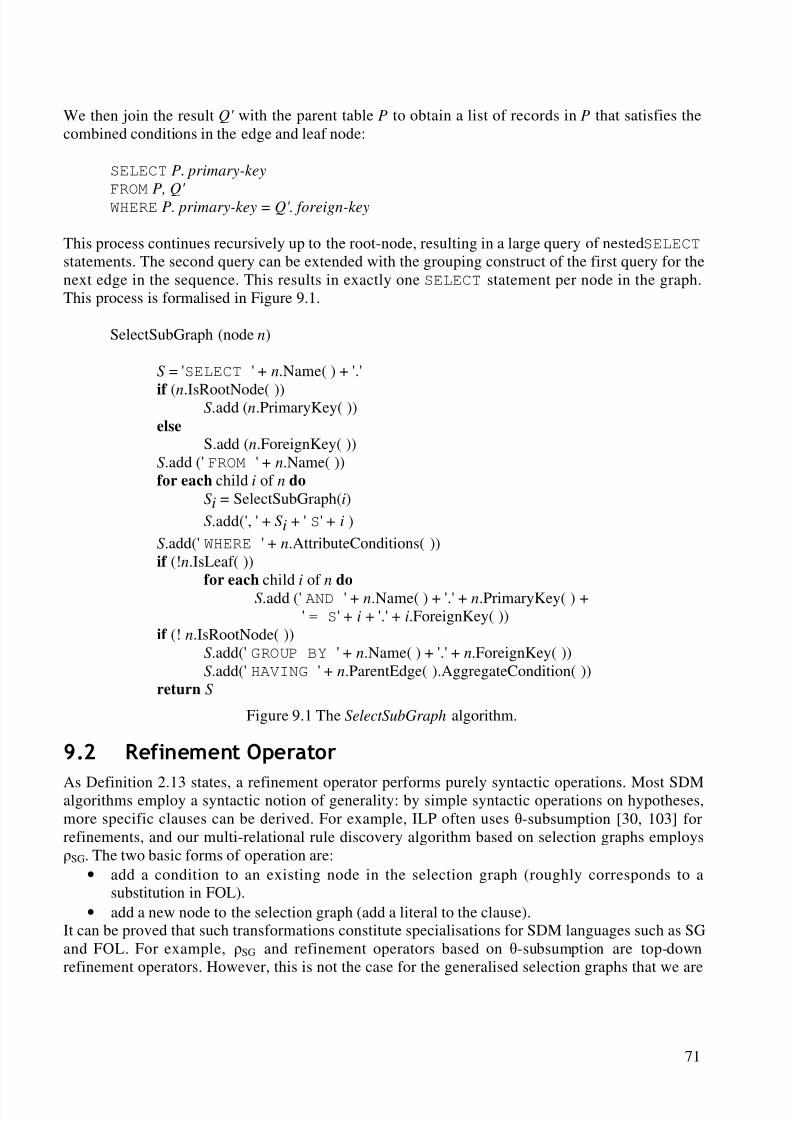
8/8/2019 Knobbe a.J. Multi-Relational Data Mining
http://slidepdf.com/reader/full/knobbe-aj-multi-relational-data-mining 82/129
71
We then join the result Q' with the parent table P to obtain a list of records in P that satisfies thecombined conditions in the edge and leaf node:
SELECT P. primary-key
FROM P, Q' WHERE P. primary-key = Q'. foreign-key
This process continues recursively up to the root-node, resulting in a large query of nested SELECT
statements. The second query can be extended with the grouping construct of the first query for thenext edge in the sequence. This results in exactly one SELECT statement per node in the graph.This process is formalised in Figure 9.1.
SelectSubGraph (node n)
S = 'SELECT ' + n.Name( ) + '.'
if (n.IsRootNode( ))S.add (n.PrimaryKey( ))else
S.add (n.ForeignKey( ))S.add (' FROM ' + n.Name( ))for each child i of n do
Si = SelectSubGraph(i)
S.add(', ' + Si + ' S' + i )
S.add(' WHERE ' + n.AttributeConditions( ))if (!n.IsLeaf( ))
for each child i of n do
S.add (' AND ' + n.Name( ) + '.' + n.PrimaryKey( ) +' = S' + i + '.' + i.ForeignKey( ))
if (! n.IsRootNode( ))S.add(' GROUP BY ' + n.Name( ) + '.' + n.ForeignKey( ))S.add(' HAVING ' + n.ParentEdge( ).AggregateCondition( ))
return S
Figure 9.1 The SelectSubGraph algorithm.
5HILQHPHQW2SHUDWRU
As Definition 2.13 states, a refinement operator performs purely syntactic operations. Most SDMalgorithms employ a syntactic notion of generality: by simple syntactic operations on hypotheses,more specific clauses can be derived. For example, ILP often uses -subsumption [30, 103] forrefinements, and our multi-relational rule discovery algorithm based on selection graphs employsSG. The two basic forms of operation are:
• add a condition to an existing node in the selection graph (roughly corresponds to asubstitution in FOL).
• add a new node to the selection graph (add a literal to the clause).It can be proved that such transformations constitute specialisations for SDM languages such as SGand FOL. For example, SG and refinement operators based on -subsumption are top-downrefinement operators. However, this is not the case for the generalised selection graphs that we are
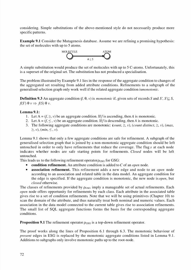
8/8/2019 Knobbe a.J. Multi-Relational Data Mining
http://slidepdf.com/reader/full/knobbe-aj-multi-relational-data-mining 83/129
72
considering. Simple substitutions of the above-mentioned style do not necessarily produce morespecific patterns.
Example 9.1 Consider the Mutagenesis database. Assume we are refining a promising hypothesis:
the set of molecules with up to 5 atoms.
A simple substitution would produce the set of molecules with up to 5 C-atoms. Unfortunately, thisis a superset of the original set. The substitution has not produced a specialisation.
The problem illustrated by Example 9.1 lies in the response of the aggregate condition to changes of the aggregated set resulting from added attribute conditions. Refinements to a subgraph of thegeneralised selection graph only work well if the related aggregate condition is monotonic.
Definition 9.3 An aggregate condition ( f , θ, v) is monotonic if, given sets of records S and S' , S' ⊆ S, f (S' ) θ v f(S) θ v.
Lemma 9.1:1. Let A = ( f , , v) be an aggregate condition. If f is ascending, then A is monotonic.2. Let A = ( f , , v) be an aggregate condition. If f is descending, then A is monotonic.3. The following aggregate conditions are monotonic: (count , , v), (count distinct , , v), (max,
, v), (min, , v).
Lemma 9.1 shows that only a few aggregate conditions are safe for refinement. A subgraph of the
generalised selection graph that is joined by a non-monotonic aggregate condition should be leftuntouched in order to only have refinements that reduce the coverage. The flag s at each nodeindicates whether nodes are safe starting points for refinements. Closed nodes will be leftuntouched.This leads us to the following refinement operator GSG for GSG:
• condition refinement. An attribute condition is added to C of an open node.• association refinement. This refinement adds a new edge and node to an open node
according to an association and related table in the data model. An aggregate condition forthe edge is specified. If the aggregate condition is monotonic, the new node is open, butclosed otherwise.
The classes of refinements provided by GSG
imply a manageable set of actual refinements. Eachopen node offers opportunity for refinements by each class. Each attribute in the associated tablegives rise to a set of condition refinements. Note that we will be using primitives (Chapter 10) toscan the domain of the attribute, and thus naturally treat both nominal and numeric values. Eachassociation in the data model connected to the current table gives rise to association refinements.The small list of SQL aggregate functions forms the basis for the corresponding aggregateconditions.
Proposition 9.1 The refinement operator GSG is a top-down refinement operator.
The proof works along the lines of Proposition 6.1 through 6.3. The monotonic behaviour of
present edges in ESG is replaced by the monotonic aggregate conditions listed in Lemma 9.1.Additions to subgraphs only involve monotonic paths up to the root-node.
MOLECULE
# 5
ATOM
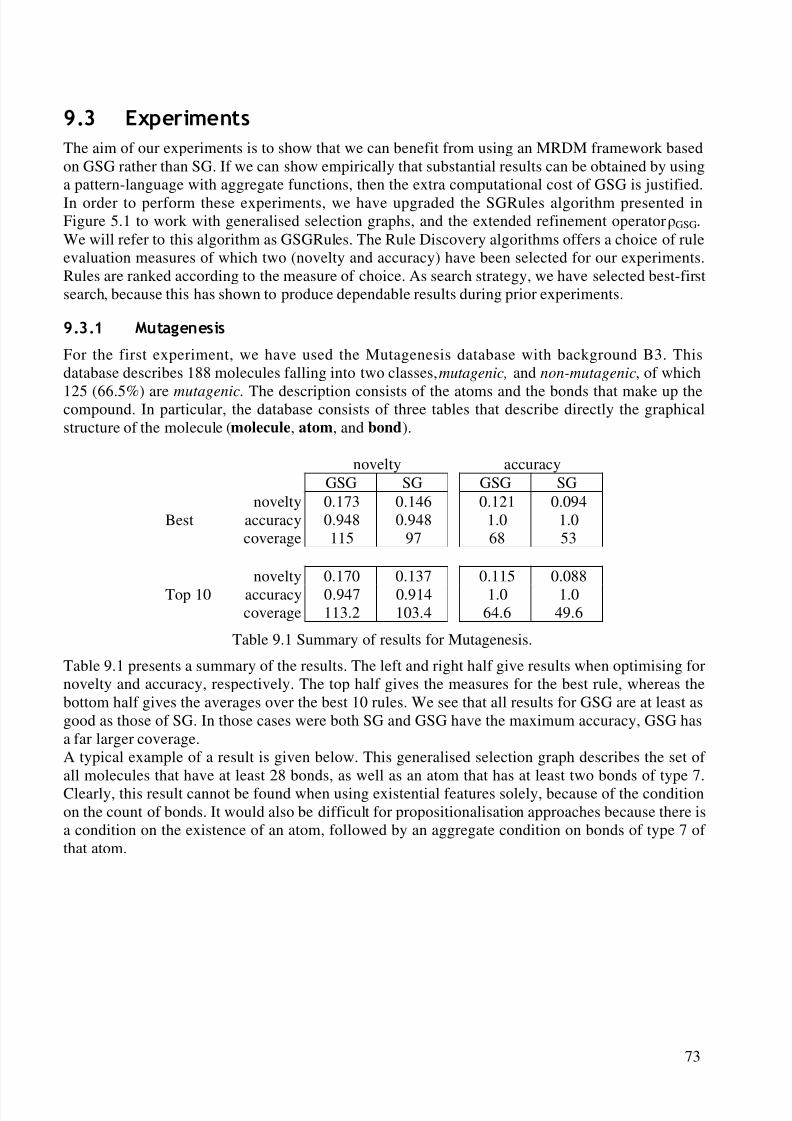
8/8/2019 Knobbe a.J. Multi-Relational Data Mining
http://slidepdf.com/reader/full/knobbe-aj-multi-relational-data-mining 84/129
73
([SHULPHQWV
The aim of our experiments is to show that we can benefit from using an MRDM framework basedon GSG rather than SG. If we can show empirically that substantial results can be obtained by usinga pattern-language with aggregate functions, then the extra computational cost of GSG is justified.In order to perform these experiments, we have upgraded the SGRules algorithm presented inFigure 5.1 to work with generalised selection graphs, and the extended refinement operator GSG.We will refer to this algorithm as GSGRules. The Rule Discovery algorithms offers a choice of ruleevaluation measures of which two (novelty and accuracy) have been selected for our experiments.Rules are ranked according to the measure of choice. As search strategy, we have selected best-firstsearch, because this has shown to produce dependable results during prior experiments.
0XWDJHQHVLV
For the first experiment, we have used the Mutagenesis database with background B3. Thisdatabase describes 188 molecules falling into two classes, mutagenic, and non-mutagenic, of which
125 (66.5%) are mutagenic. The description consists of the atoms and the bonds that make up thecompound. In particular, the database consists of three tables that describe directly the graphicalstructure of the molecule (molecule, atom, and bond).
novelty accuracyGSG SG GSG SG
novelty 0.173 0.146 0.121 0.094Best accuracy 0.948 0.948 1.0 1.0
coverage 115 97 68 53
novelty 0.170 0.137 0.115 0.088
Top 10 accuracy 0.947 0.914 1.0 1.0coverage 113.2 103.4 64.6 49.6
Table 9.1 Summary of results for Mutagenesis.
Table 9.1 presents a summary of the results. The left and right half give results when optimising fornovelty and accuracy, respectively. The top half gives the measures for the best rule, whereas thebottom half gives the averages over the best 10 rules. We see that all results for GSG are at least asgood as those of SG. In those cases were both SG and GSG have the maximum accuracy, GSG hasa far larger coverage.A typical example of a result is given below. This generalised selection graph describes the set of all molecules that have at least 28 bonds, as well as an atom that has at least two bonds of type 7.Clearly, this result cannot be found when using existential features solely, because of the conditionon the count of bonds. It would also be difficult for propositionalisation approaches because there isa condition on the existence of an atom, followed by an aggregate condition on bonds of type 7 of that atom.
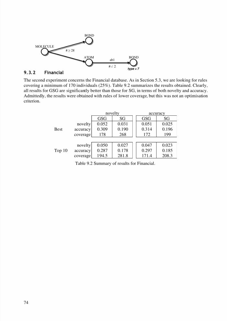
8/8/2019 Knobbe a.J. Multi-Relational Data Mining
http://slidepdf.com/reader/full/knobbe-aj-multi-relational-data-mining 85/129
74
)LQDQFLDO
The second experiment concerns the Financial database. As in Section 5.3, we are looking for rulescovering a minimum of 170 individuals (25%). Table 9.2 summarizes the results obtained. Clearly,all results for GSG are significantly better than those for SG, in terms of both novelty and accuracy.Admittedly, the results were obtained with rules of lower coverage, but this was not an optimisationcriterion.
novelty accuracyGSG SG GSG SG
novelty 0.052 0.031 0.051 0.025Best accuracy 0.309 0.190 0.314 0.196
coverage 178 268 172 199
novelty 0.050 0.027 0.047 0.023Top 10 accuracy 0.287 0.178 0.297 0.185
coverage 194.5 281.8 171.4 208.3
Table 9.2 Summary of results for Financial.
MOLECULE
ab1
BOND
# 28
ATOM
# 2type = 7
BOND
8/8/2019 Knobbe a.J. Multi-Relational Data Mining
http://slidepdf.com/reader/full/knobbe-aj-multi-relational-data-mining 86/129
75
05'03ULPLWLYHV
$Q05'0$UFKLWHFWXUH
Data Mining, and specifically the multi-relational variety, is a computation-intensive activity.Especially with serious applications of industrial size, a lot of data needs to be processed and
scanned multiple times, in order to validate the large number of hypotheses generated by thealgorithms such as covered in this text. We demand implementations of these algorithms to be atleast moderately efficient and more importantly scalable, that is to perform predictively withincreasing data volumes. These demands force us to pay attention to the architecture of suchimplementations. In this section we propose a three-tiered Client/Server architecture that satisfiesthese demands. It has been applied with success in Propositional Data Mining software [42, 46, 55].An important subject in Data Mining architecture is how data access is organised. The remainingsections of this chapter are therefore devoted to multi-relational data mining primitives (see alsoSection 5.2) that address this subject.The architecture consists of three tiers (see Figure 10.1): the presentation tier , the Data Mining tier
and the database tier . Each tier will typically run on a separate workstation that is tuned towards thespecific needs of the tier in question. For example the database tier will ideally run on a large serverwith ample main memory and fast access to secondary storage, whereas for the presentation tier, aregular desktop machine will suffice. Although separate workstations for each tier are optimal,several tiers can be run on a single machine. The presentation and Data Mining tier are an obviouschoice, as they both have moderate computation requirements. The MRDM package Safarii followsthis scheme.The database tier has exclusive access to the data. It is responsible for the actual scanning of thisdata, and answering queries about the frequency of certain patterns. Furthermore its task is to findan efficient way of processing the many (similar) queries. The Data Mining tier is responsible forguiding the search, and producing interesting hypotheses for the database tier to test. It will often
consist of an MRDM kernel that deals with the basics of MRDM, such as the representation of datamodels, selection graphs and refinements etc., as well as a number of search algorithms that
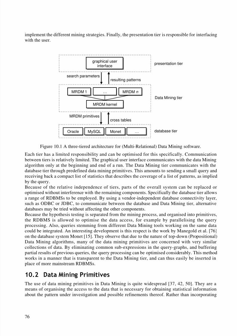
8/8/2019 Knobbe a.J. Multi-Relational Data Mining
http://slidepdf.com/reader/full/knobbe-aj-multi-relational-data-mining 87/129
76
implement the different mining strategies. Finally, the presentation tier is responsible for interfacingwith the user.
Figure 10.1 A three-tiered architecture for (Multi-Relational) Data Mining software.
Each tier has a limited responsibility and can be optimised for this specifically. Communicationbetween tiers is relatively limited. The graphical user interface communicates with the data Miningalgorithm only at the beginning and end of a run. The Data Mining tier communicates with thedatabase tier through predefined data mining primitives. This amounts to sending a small query and
receiving back a compact list of statistics that describes the coverage of a list of patterns, as impliedby the query.Because of the relative independence of tiers, parts of the overall system can be replaced oroptimised without interference with the remaining components. Specifically the database tier allowsa range of RDBMSs to be employed. By using a vendor-independent database connectivity layer,such as ODBC or JDBC, to communicate between the database and Data Mining tier, alternativedatabases may be tried without affecting the other components.Because the hypothesis testing is separated from the mining process, and organised into primitives,the RDBMS is allowed to optimise the data access, for example by parallelising the queryprocessing. Also, queries stemming from different Data Mining tools working on the same datacould be integrated. An interesting development is this respect is the work by Manegold et al. [76]
on the database system Monet [15]. They observe that due to the nature of top-down (Propositional)Data Mining algorithms, many of the data mining primitives are concerned with very similarcollections of data. By eliminating common sub-expressions in the query-graphs, and bufferingpartial results of previous queries, the query processing can be optimised considerably. This methodworks in a manner that is transparent to the Data Mining tier, and can thus easily be inserted inplace of more mainstream RDBMSs.
'DWD0LQLQJ3ULPLWLYHV
The use of data mining primitives in Data Mining is quite widespread [37, 42, 50]. They are ameans of organising the access to the data that is necessary for obtaining statistical information
about the pattern under investigation and possible refinements thereof. Rather than incorporating
…
MRDM kernel
MRDM n MRDM 1
MySQL Monet …Oracle
graphical userinterface
resulting patternssearch parameters
cross tablesMRDM primitives
database tier
Data Mining tier
presentation tier
8/8/2019 Knobbe a.J. Multi-Relational Data Mining
http://slidepdf.com/reader/full/knobbe-aj-multi-relational-data-mining 88/129
77
random access to individual pieces of data in the Data Mining algorithm, a small set of queries isdefined, typically in SQL, that produce the necessary summaries to guide the search algorithm. Thefollowing sections provide an overview of the different multi-relational data mining primitivesrequired to support the variety of MRDM approaches introduced in the previous chapters.
Data mining primitives have a number of important benefits:• they represent a concise summary of both the necessary and sufficient information requiredto judge a pattern. They provide the efficient communication that is typical of a goodClient/Server architecture.
• a range of possible refinements for a given pattern is investigated by a single primitive. TheRDBMS is thus given an opportunity to optimise multiple very similar scans of the data.
• deciding which actual refinements will be considered by the search process is left to theRDBMS to some extent. When considering, for example, a condition refinement on a givenselection graph for a given node and attribute, the primitive will list all the values that areavailable for this attribute under these circumstances. This allows algorithms to consider thecorrect set of condition refinements, without a priori knowledge of the domain of the
attribute. Particularly with aggregate functions, where the domain of the function dependsentirely on the aggregated set, a data-driven generation of possible aggregate conditions isessential.
Although a large variety of primitives can be defined, we will be using primitives that producecounts. These counts will be in terms of individuals, i.e. in terms of records in the target table. Eachcount thus represents the coverage of a specific subgroup.We will be considering primitives in two styles. In the first style, we will be treating selectiongraphs as specifications of joins over the tables involved. Because we can think of both theexistential constraints as well as the attribute conditions as selections on the Cartesian product of the tables, the whole selection can be expressed in a single SELECT statement. This will produceSQL statements similar to those introduced in Chapter 4. The second style of primitives is moreapplicable if patterns involve aggregate functions. Here we treat (generalised) selection graphs asrecursive definitions of groups of records associated with each node. We will be using nestedqueries rather than joins to produce the collective counts over individuals.In the next sections we will consider primitives for each refinement, for selection graphs, extendedselection graphs, and generalised selection graphs in turn.
6HOHFWLRQ*UDSKV
The following four data mining primitives can be used to support the discovery of selection graphsas defined in Chapter 4. The first two primitives provide the necessary counts to test associationrefinements. The next pair supports condition refinements.
$VVRFLDWLRQ5HILQHPHQW
The following primitive counts the number of individuals covered by a given selection graph. Itbasically counts over a selection of the Cartesian product of tables involved (see theTranslateSelectionGraph algorithm in Section 4.2). As individuals can occur multiple times in thisselection, we have to apply the DISTINCT operator. Although the CountSelection primitive can beused to compute the coverage of arbitrary selection graphs, we will mainly use it to assess theinterestingness of an association refinement by running the primitive on the selection graphproduced by the association refinement. This count is typically compared to the coverage of theselection graph prior to refinement, or to that of the empty selection graph.
8/8/2019 Knobbe a.J. Multi-Relational Data Mining
http://slidepdf.com/reader/full/knobbe-aj-multi-relational-data-mining 89/129
78
CountSelection:
SELECT COUNT(DISTINCT t 0. primary_key)
FROM table_list
WHERE join_list AND condition_list
Instead of working with the coverage of subgroups, we will often be interested in the distribution of values for the target attribute within the subgroup. From these counts, and the overall distribution,we can compute the value of a range of evaluation measures, as was briefly demonstrated in Section5.2. The Histogram primitive produces this list of counts for association refinements. Note that thesum of the counts in the resulting histogram is equal to the result of the CountSelection primitive.
Histogram:
SELECT t 0.target , COUNT(DISTINCT t 0. primary_key)
FROM table_list
WHERE join_list AND condition_list
GROUP BY t 0.target
1RPLQDO&RQGLWLRQ5HILQHPHQW
Similar to the Histogram primitive, the NominalCrossTable primitive produces counts pertaining tothe distribution of values for the target attribute. In this case however, we are interested in how thisdistribution depends on the value of a nominal attribute t i.c j in one of the tables appearing in theselection graph at hand. The NominalCrossTable primitive will list all pairs of values that occur inthe database, along with the number of individuals this combination occurs in. The resulting crosstable can be used to compute a range of statistical measures describing the dependency betweenthese two attributes. Note that the sum of these counts can exceed the support of the given multi-
relational pattern, if the attribute t i.c j is in a table that is not the target table. This is because multiplerecords, with different values for the selected attribute, may correspond to a single record in thetarget table, causing this record to contribute to multiple counts in the cross table.The NominalCrossTable primitive can be used to evaluate a set of condition refinements involvingthe condition t i.c j = x. Each count in the cross table describes the number of individuals for aparticular target value, as if the condition refinement were already executed for a particular value of t i.c j. The primitive will only return combinations of values that actually appear in the database.
NominalCrossTable:
SELECT t 0.target , t i.c j, COUNT(DISTINCT t 0. primary_key)
FROM table_list
WHERE join_list AND condition_list
GROUP BY t 0.target, t i.c j
Example 10.1 Consider the following NominalCrossTable primitive introduced in Section 5.2:
SELECT molecule.mutagenic, atom.element,
COUNT(DISTINCT molecule.id)
FROM molecule, atom
WHERE molecule.id = atom.molecule_id
GROUP BY molecule.mutagenic, atom.element
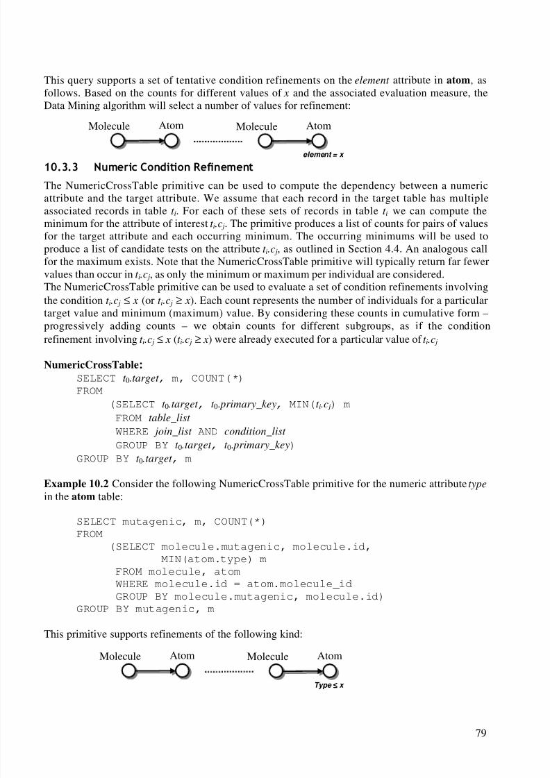
8/8/2019 Knobbe a.J. Multi-Relational Data Mining
http://slidepdf.com/reader/full/knobbe-aj-multi-relational-data-mining 90/129
79
This query supports a set of tentative condition refinements on the element attribute in atom, asfollows. Based on the counts for different values of x and the associated evaluation measure, theData Mining algorithm will select a number of values for refinement:
1XPHULF&RQGLWLRQ5HILQHPHQW
The NumericCrossTable primitive can be used to compute the dependency between a numericattribute and the target attribute. We assume that each record in the target table has multipleassociated records in table t i. For each of these sets of records in table t i we can compute theminimum for the attribute of interest t i.c j. The primitive produces a list of counts for pairs of valuesfor the target attribute and each occurring minimum. The occurring minimums will be used toproduce a list of candidate tests on the attribute t i.c j, as outlined in Section 4.4. An analogous callfor the maximum exists. Note that the NumericCrossTable primitive will typically return far fewer
values than occur in t i.c j, as only the minimum or maximum per individual are considered.The NumericCrossTable primitive can be used to evaluate a set of condition refinements involvingthe condition t i.c j ≤ x (or t i.c j ≥ x). Each count represents the number of individuals for a particulartarget value and minimum (maximum) value. By considering these counts in cumulative form –progressively adding counts – we obtain counts for different subgroups, as if the conditionrefinement involving t i.c j ≤ x (t i.c j ≥ x) were already executed for a particular value of t i.c j
NumericCrossTable:SELECT t 0.target , m, COUNT(*)
FROM
(SELECT t 0.target , t 0. primary_key, MIN(t i.c j) mFROM table_list
WHERE join_list AND condition_list
GROUP BY t 0.target , t 0. primary_key)
GROUP BY t 0.target , m
Example 10.2 Consider the following NumericCrossTable primitive for the numeric attribute type
in the atom table:
SELECT mutagenic, m, COUNT(*)
FROM
(SELECT molecule.mutagenic, molecule.id,MIN(atom.type) m
FROM molecule, atom
WHERE molecule.id = atom.molecule_id
GROUP BY molecule.mutagenic, molecule.id)
GROUP BY mutagenic, m
This primitive supports refinements of the following kind:
AtomMolecule AtomMolecule
element = x
AtomMolecule AtomMolecule
Type ≤≤≤≤ x
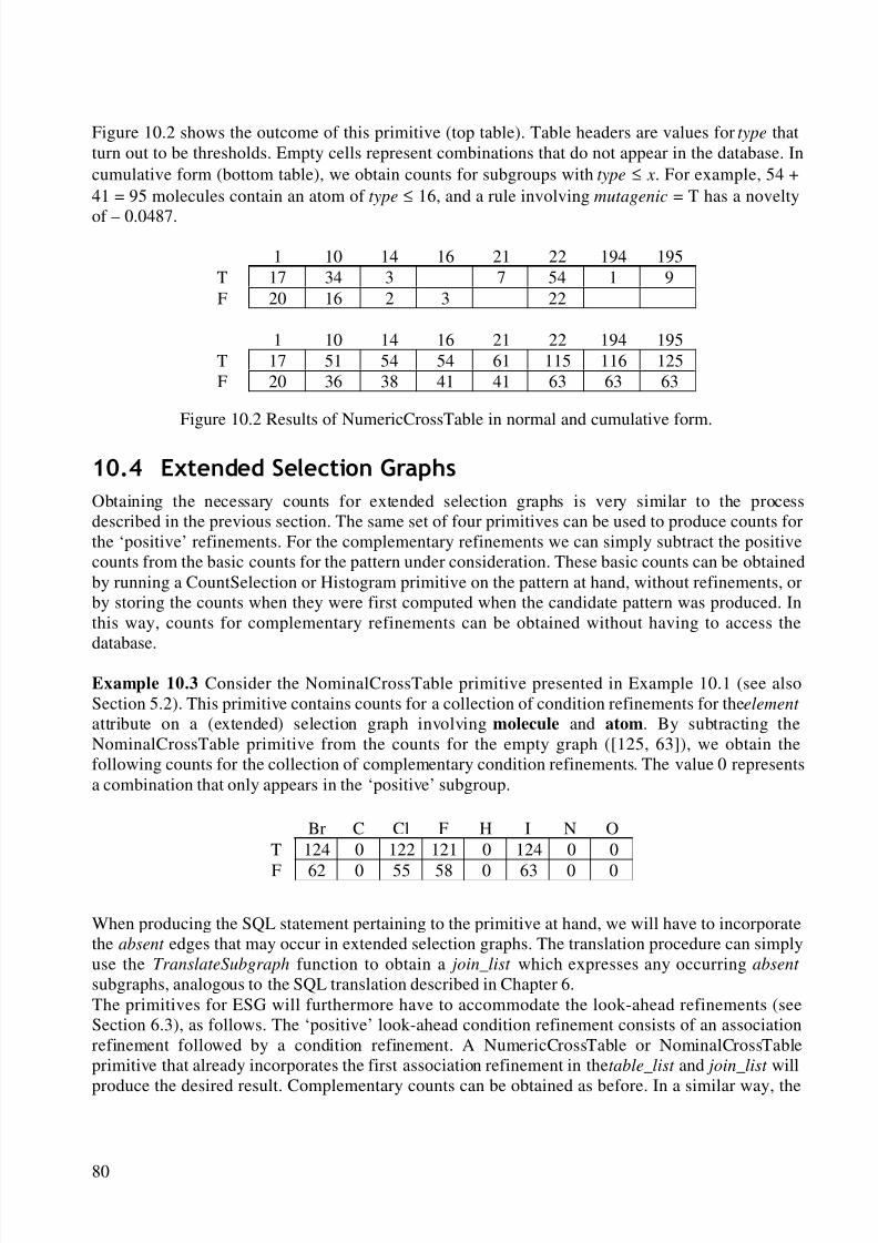
8/8/2019 Knobbe a.J. Multi-Relational Data Mining
http://slidepdf.com/reader/full/knobbe-aj-multi-relational-data-mining 91/129
80
Figure 10.2 shows the outcome of this primitive (top table). Table headers are values for type thatturn out to be thresholds. Empty cells represent combinations that do not appear in the database. Incumulative form (bottom table), we obtain counts for subgroups with type ≤ x. For example, 54 +41 = 95 molecules contain an atom of type ≤ 16, and a rule involving mutagenic = T has a novelty
of – 0.0487.
1 10 14 16 21 22 194 195T 17 34 3 7 54 1 9F 20 16 2 3 22
1 10 14 16 21 22 194 195T 17 51 54 54 61 115 116 125F 20 36 38 41 41 63 63 63
Figure 10.2 Results of NumericCrossTable in normal and cumulative form.
([WHQGHG6HOHFWLRQ*UDSKV
Obtaining the necessary counts for extended selection graphs is very similar to the processdescribed in the previous section. The same set of four primitives can be used to produce counts forthe ‘positive’ refinements. For the complementary refinements we can simply subtract the positivecounts from the basic counts for the pattern under consideration. These basic counts can be obtainedby running a CountSelection or Histogram primitive on the pattern at hand, without refinements, orby storing the counts when they were first computed when the candidate pattern was produced. Inthis way, counts for complementary refinements can be obtained without having to access thedatabase.
Example 10.3 Consider the NominalCrossTable primitive presented in Example 10.1 (see alsoSection 5.2). This primitive contains counts for a collection of condition refinements for the element
attribute on a (extended) selection graph involving molecule and atom. By subtracting theNominalCrossTable primitive from the counts for the empty graph ([125, 63]), we obtain thefollowing counts for the collection of complementary condition refinements. The value 0 representsa combination that only appears in the ‘positive’ subgroup.
When producing the SQL statement pertaining to the primitive at hand, we will have to incorporatethe absent edges that may occur in extended selection graphs. The translation procedure can simplyuse the TranslateSubgraph function to obtain a join_list which expresses any occurring absent
subgraphs, analogous to the SQL translation described in Chapter 6.The primitives for ESG will furthermore have to accommodate the look-ahead refinements (seeSection 6.3), as follows. The ‘positive’ look-ahead condition refinement consists of an associationrefinement followed by a condition refinement. A NumericCrossTable or NominalCrossTableprimitive that already incorporates the first association refinement in the table_list and join_list will
produce the desired result. Complementary counts can be obtained as before. In a similar way, the
Br C Cl F H I N OT 124 0 122 121 0 124 0 0
F 62 0 55 58 0 63 0 0
8/8/2019 Knobbe a.J. Multi-Relational Data Mining
http://slidepdf.com/reader/full/knobbe-aj-multi-relational-data-mining 92/129
81
look-ahead association refinement can be validated by a Histogram primitive that includes the twonew tables in the table_list and join_list .
*HQHUDOLVHG6HOHFWLRQ*UDSKV
We start by repeating the basic process of recursively selecting groups of records, as described inChapter 9 and Figure 9.1. This process will be the basis for the primitives related to generalisedselection graphs. Every node in a generalised selection graph represents a selection of records in theassociated table. If we start at the leaves of the graph and work back to the root, respecting all theselection conditions, we can compute the selection of records in the target table. This is achieved asfollows. First we produce a list of groups of records in a table Q at a leaf node by testing on theaggregate condition. Each group is identified by the value of the foreign key:
SELECT foreign_key
FROM Q
WHERE attribute_conditionsGROUP BY foreign_key
HAVING aggregate_condition
We then join the result Q' with the parent table P to obtain a list of records in P that adheres to thecombined conditions in the edge and leaf node:
SELECT P. primary_key
FROM P, Q'
WHERE P.primary_key = Q'. foreign_key
This process continues recursively up to the root-node, resulting in a large query C of nestedSELECT statements. The different primitives are all variations on this basic construct.
$VVRFLDWLRQ5HILQHPHQW
The CountSelection primitive simply counts the number of individuals covered by the generalisedselection graph, as in the case of selection graphs:
CountSelection:SELECT COUNT(*)
FROM C
The Histogram primitive computes the distribution of values of the target attribute within the set of individuals covered by the generalised selection graph, as before.
Histogram:
SELECT target , COUNT(*)
FROM C
GROUP BY target
1RPLQDO&RQGLWLRQ5HILQHPHQW
As before, the NominalCrossTable primitive can be used to determine the effect of a conditionrefinement involving a nominal attribute on the distribution of target values. All pairs of nominal
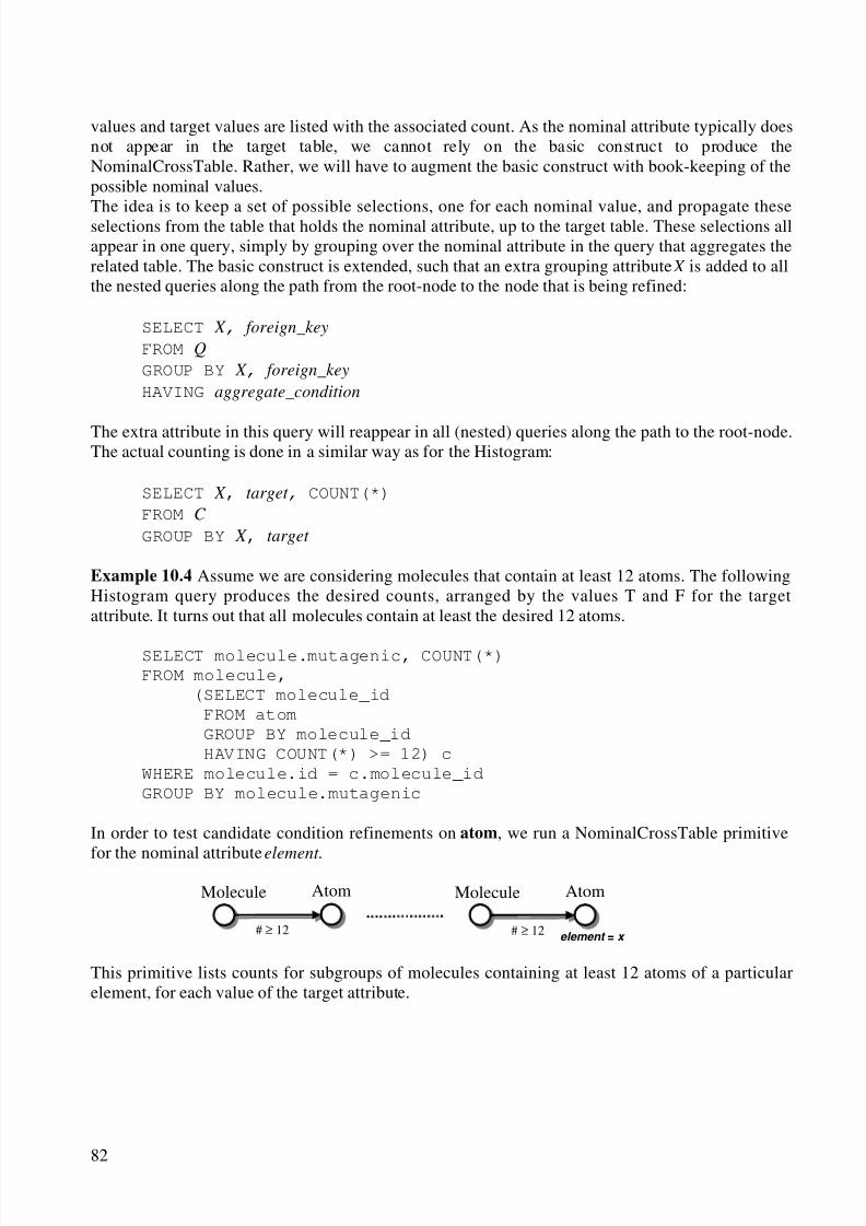
8/8/2019 Knobbe a.J. Multi-Relational Data Mining
http://slidepdf.com/reader/full/knobbe-aj-multi-relational-data-mining 93/129
82
values and target values are listed with the associated count. As the nominal attribute typically doesnot appear in the target table, we cannot rely on the basic construct to produce theNominalCrossTable. Rather, we will have to augment the basic construct with book-keeping of thepossible nominal values.
The idea is to keep a set of possible selections, one for each nominal value, and propagate theseselections from the table that holds the nominal attribute, up to the target table. These selections allappear in one query, simply by grouping over the nominal attribute in the query that aggregates therelated table. The basic construct is extended, such that an extra grouping attribute X is added to allthe nested queries along the path from the root-node to the node that is being refined:
SELECT X , foreign_key
FROM Q
GROUP BY X , foreign_key
HAVING aggregate_condition
The extra attribute in this query will reappear in all (nested) queries along the path to the root-node.The actual counting is done in a similar way as for the Histogram:
SELECT X , target , COUNT(*)
FROM C
GROUP BY X , target
Example 10.4 Assume we are considering molecules that contain at least 12 atoms. The followingHistogram query produces the desired counts, arranged by the values T and F for the targetattribute. It turns out that all molecules contain at least the desired 12 atoms.
SELECT molecule.mutagenic, COUNT(*)
FROM molecule,
(SELECT molecule_id
FROM atom
GROUP BY molecule_id
HAVING COUNT(*) >= 12) c
WHERE molecule.id = c.molecule_id
GROUP BY molecule.mutagenic
In order to test candidate condition refinements on atom, we run a NominalCrossTable primitive
for the nominal attribute element .
This primitive lists counts for subgroups of molecules containing at least 12 atoms of a particularelement, for each value of the target attribute.
# ≥ 12
AtomMolecule
# ≥ 12
AtomMolecule
element = x
8/8/2019 Knobbe a.J. Multi-Relational Data Mining
http://slidepdf.com/reader/full/knobbe-aj-multi-relational-data-mining 94/129
83
SELECT molecule.mutagenic, c.element, COUNT(*)
FROM molecule,
(SELECT element, molecule_id
FROM atom
GROUP BY element, molecule_id
HAVING COUNT(*) >= 12) c
WHERE molecule.id = c.molecule_id
GROUP BY c.element, molecule.mutagenic
This query produces the following results. For example, there is a single non-mutagenic moleculethat has at least 12 hydrogen atoms. Note that only carbon and hydrogen appear frequent enoughper molecule to appear in the result.
C HT 112 12
F 18 1 1XPHULF&RQGLWLRQ5HILQHPHQW
As before, the NumericCrossTable primitive can be used to obtain a list of suitable numericrefinements together with the effect this has on the class-distribution. It is very similar to theNominalCrossTable, but requires yet a little more book-keeping. This is because a given record maysatisfy a number of numeric conditions, whereas it will only satisfy a single nominal condition. Theprocess starts by producing a list of combinations of records and thresholds, and then proceeds asbefore. Note that there is a version of the NummericCrossTable for each operator ≤ and ≥.The NumericCrossTable primitive for GSG works differently from its SG counterpart. Because theGSG primitives do not work on selections of the Cartesian product, we can not rely on theminimum and maximum as before. Rather we will have to keep track of different tentative numericthresholds and propagate the associated selections of records up to the target table.
SELECT b. X , a. foreign_key
FROM Q a, (SELECT DISTINCT X FROM Q) b
WHERE a. X <= b. X
GROUP BY b. X , a. foreign_key
HAVING aggregate_condition
Example 10.5 Assume we are looking for subgroups of molecules that contain at least 12 atoms
again, and are interested in the effect of adding a numeric condition on the atoms. The followingprimitive produces counts for condition refinements involving atom.type ≤ x. The query listssuitable values for x, along with the number of individuals that satisfy these conditions.
8/8/2019 Knobbe a.J. Multi-Relational Data Mining
http://slidepdf.com/reader/full/knobbe-aj-multi-relational-data-mining 95/129
84
SELECT molecule.mutagenic, c.type, COUNT(*)
FROM molecule,
(SELECT b.type, a.molecule_id
FROM atom a, (SELECT DISTINCT type FROM atom) b
WHERE a.type <= b.type
GROUP BY b.type, a.molecule_id
HAVING COUNT(*) >= 12) c
WHERE molecule.id = c.molecule_id
GROUP BY c.type, molecule.mutagenic
This NumericCrossTable primitive produces the following results. Values above the columnsindicate thresholds for type.
3 8 10 14 16 19 21 25 26 27 …T 12 12 20 20 23 23 28 119 119 121 …
F 1 1 4 4 6 6 6 50 52 52 …
$JJUHJDWH&URVV7DEOH
The AggregateCrossTable is our most elaborate primitive. It can be used to obtain a list of suitableaggregate conditions for a given aggregate function. The AggregateCrossTable primitivedemonstrates the power of data mining primitives because the list of suitable conditions can only beobtained through extensive analysis of the database. It cannot be obtained from the domainknowledge or a superficial scan when starting the mining process.We will treat candidate aggregate conditions as virtual attributes of the parent table. A first query isapplied to produce this virtual attribute. Then the NumericCrossTable primitive is applied with thevirtual attribute as the candidate. The first step looks as follows:
SELECT foreign_key, aggregate_function
FROM Q
GROUP BY foreign_key
Example 10.6 Assume we are working with the subgroup of molecules that contain at least 12atoms, as in Example 10.4 and 10.5. If we are considering an association refinement involvingcounting over one of the associations between atom and bond, we can apply the above query. Thisquery produces a virtual numeric attribute in atom, representing the number of associated bonds:
SELECT atom1, COUNT(*) c
FROM bond
GROUP BY atom1
We can now run the NumericCrossTable primitive, as we did before on the type attribute.
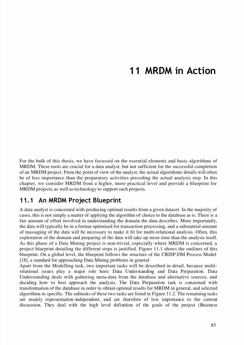
8/8/2019 Knobbe a.J. Multi-Relational Data Mining
http://slidepdf.com/reader/full/knobbe-aj-multi-relational-data-mining 96/129
85
05'0LQ$FWLRQ
For the bulk of this thesis, we have focussed on the essential elements and basic algorithms of MRDM. These tools are crucial for a data analyst, but not sufficient for the successful completionof an MRDM project. From the point of view of the analyst, the actual algorithmic details will oftenbe of less importance than the preparatory activities preceding the actual analysis step. In thischapter, we consider MRDM from a higher, more practical level and provide a blueprint forMRDM projects, as well as technology to support such projects.
$Q05'03URMHFW%OXHSULQW
A data analyst is concerned with producing optimal results from a given dataset. In the majority of cases, this is not simply a matter of applying the algorithm of choice to the database as is. There is afair amount of effort involved in understanding the domain the data describes. More importantly,the data will typically be in a format optimised for transaction processing, and a substantial amountof massaging of the data will be necessary to make it fit for multi-relational analysis. Often, thisexploration of the domain and preparing of the data will take up more time than the analysis itself.
As this phase of a Data Mining project is non-trivial, especially where MRDM is concerned, aproject blueprint detailing the different steps is justified. Figure 11.1 shows the outlines of thisblueprint. On a global level, the blueprint follows the structure of the CRISP-DM Process Model[18], a standard for approaching Data Mining problems in general.Apart from the Modelling task, two important tasks will be described in detail, because multi-relational issues play a major role here: Data Understanding and Data Preparation. DataUnderstanding deals with gathering meta-data from the database and alternative sources, anddeciding how to best approach the analysis. The Data Preparation task is concerned withtransformation of the database in order to obtain optimal results for MRDM in general, and selectedalgorithms in specific. The subtasks of these two tasks are listed in Figure 11.2. The remaining tasksare mainly representation-independent, and are therefore of less importance to the currentdiscussion. They deal with the high level definition of the goals of the project (Business
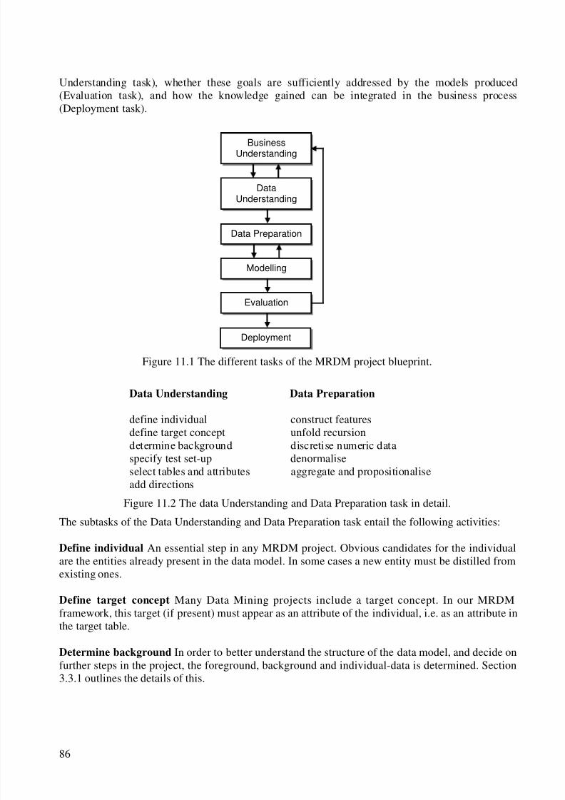
8/8/2019 Knobbe a.J. Multi-Relational Data Mining
http://slidepdf.com/reader/full/knobbe-aj-multi-relational-data-mining 97/129
86
Understanding task), whether these goals are sufficiently addressed by the models produced(Evaluation task), and how the knowledge gained can be integrated in the business process(Deployment task).
Figure 11.1 The different tasks of the MRDM project blueprint.
Data Understanding Data Preparation
define individual construct featuresdefine target concept unfold recursiondetermine background discretise numeric dataspecify test set-up denormaliseselect tables and attributes aggregate and propositionaliseadd directions
Figure 11.2 The data Understanding and Data Preparation task in detail.
The subtasks of the Data Understanding and Data Preparation task entail the following activities:
Define individual An essential step in any MRDM project. Obvious candidates for the individual
are the entities already present in the data model. In some cases a new entity must be distilled fromexisting ones.
Define target concept Many Data Mining projects include a target concept. In our MRDMframework, this target (if present) must appear as an attribute of the individual, i.e. as an attribute inthe target table.
Determine background In order to better understand the structure of the data model, and decide onfurther steps in the project, the foreground, background and individual-data is determined. Section3.3.1 outlines the details of this.
BusinessUnderstanding
DataUnderstanding
Data Preparation
Modelling
Evaluation
Deployment
8/8/2019 Knobbe a.J. Multi-Relational Data Mining
http://slidepdf.com/reader/full/knobbe-aj-multi-relational-data-mining 98/129
87
Specify test set-up Any serious Data Mining project involves validating the quality of the models.Validation is typically achieved by splitting the database into multiple samples, then building andtesting the model on separate samples, referred to as the training and test set. The most commonprocedure, n-fold cross-validation, involves n mutually exclusive samples. The Data Mining
algorithm is then applied n times to the union of n-1 samples with the resulting model tested on theremaining sample.Clearly, any sampling in MRDM should be done on the level of the individual. This can easily bedone if the foreground and the individual-data coincide. Care will have to be taken if tables appearin the foreground that are not individual-specific. This dynamic data that is shared by samples canbest be removed from the analysis.
Select tables and attributes Selecting a subset of the available information for analysis is a simple,yet important and frequent operation in Data Mining projects. It is mainly used as it is typicallyused in Propositional Data Mining: to restrict the scope of the analysis, to reduce the analysis time,to remove information that directly depends on the target concept, or to remove data that is shared
by individuals.
Add directions Section 3.3.2 explains how directions can be an important form of declarative biasthat can help make the search more efficient or relevant.
The Data Preparation task consists of the following subtasks:
Construct features A database designed for transaction processing will generally not contain anyredundancy. For analysis however, having multiple views on the same information may be valuablebecause not all of these alternative representations may demonstrate the desired dependencies.Feature construction involves the definition of new attributes (or even tables) as a function of
existing data, with the aim of providing the Data Mining tool with such alternative views. Featureconstruction is an important means of incorporating domain knowledge into the analysis. As anexample, think of a database of objects in the physical world, where derived attributes such assurface area, volume or density can be just as informative as the primary dimensions of the objects.The validity of specific arithmetic functions of attributes must be made specific.
Unfold recursion A special form of feature construction deals with recursive structures. Recursionis an important challenge and research topic in ILP. Most methods aim at discovering opportunitiesfor applying recursive patterns in databases of which little is know about the data model. In MRDMhowever, a detailed data model is generally available, and recursive structures in the data can beeasily identified by locating possible cycles in the data model. Because our MRDM framework does
not support recursive patterns, the unfold recursion subtask involves eliciting essential informationfrom the recursive structure. The extracted features capture as much of the original information,while respecting the limitations of non-recursive algorithms.Recursive fragments of a data model typically represent datastructures such as lists, trees or sets.Although the data representation is complete, it hides a number of properties of the datastructure(such as its size) to general purpose Data Mining algorithms. The aim of the unfold recursion task isto transform the data, such that important and promising features are made explicit, at the cost of losing some of the complete recursive description. This entails defining a number of new (ideallyintensional) tables that replace the recursive fragment. Because these definitions need to considerthe recursive structure, we will have to use a procedural language or, often vendor-specific,recursive constructs in SQL. Full support for recursion as included in the SQL3 definition iscurrently not provided by the major RDBMSs [101].
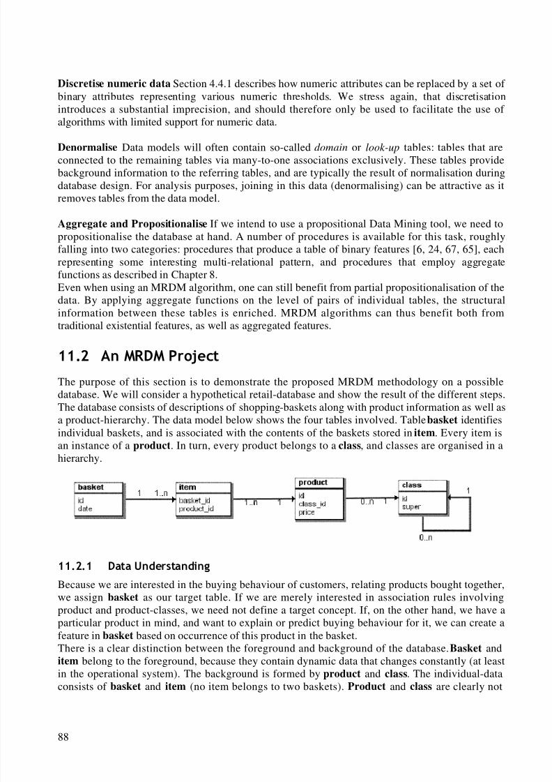
8/8/2019 Knobbe a.J. Multi-Relational Data Mining
http://slidepdf.com/reader/full/knobbe-aj-multi-relational-data-mining 99/129
88
Discretise numeric data Section 4.4.1 describes how numeric attributes can be replaced by a set of binary attributes representing various numeric thresholds. We stress again, that discretisationintroduces a substantial imprecision, and should therefore only be used to facilitate the use of algorithms with limited support for numeric data.
Denormalise Data models will often contain so-called domain or look-up tables: tables that areconnected to the remaining tables via many-to-one associations exclusively. These tables providebackground information to the referring tables, and are typically the result of normalisation duringdatabase design. For analysis purposes, joining in this data (denormalising) can be attractive as itremoves tables from the data model.
Aggregate and Propositionalise If we intend to use a propositional Data Mining tool, we need topropositionalise the database at hand. A number of procedures is available for this task, roughlyfalling into two categories: procedures that produce a table of binary features [6, 24, 67, 65], eachrepresenting some interesting multi-relational pattern, and procedures that employ aggregate
functions as described in Chapter 8.Even when using an MRDM algorithm, one can still benefit from partial propositionalisation of thedata. By applying aggregate functions on the level of pairs of individual tables, the structuralinformation between these tables is enriched. MRDM algorithms can thus benefit both fromtraditional existential features, as well as aggregated features.
$Q05'03URMHFW
The purpose of this section is to demonstrate the proposed MRDM methodology on a possibledatabase. We will consider a hypothetical retail-database and show the result of the different steps.
The database consists of descriptions of shopping-baskets along with product information as well asa product-hierarchy. The data model below shows the four tables involved. Table basket identifiesindividual baskets, and is associated with the contents of the baskets stored in item. Every item isan instance of a product. In turn, every product belongs to a class, and classes are organised in ahierarchy.
'DWD8QGHUVWDQGLQJ
Because we are interested in the buying behaviour of customers, relating products bought together,we assign basket as our target table. If we are merely interested in association rules involvingproduct and product-classes, we need not define a target concept. If, on the other hand, we have aparticular product in mind, and want to explain or predict buying behaviour for it, we can create afeature in basket based on occurrence of this product in the basket.There is a clear distinction between the foreground and background of the database. Basket anditem belong to the foreground, because they contain dynamic data that changes constantly (at leastin the operational system). The background is formed by product and class. The individual-data
consists of basket and item (no item belongs to two baskets). Product and class are clearly not
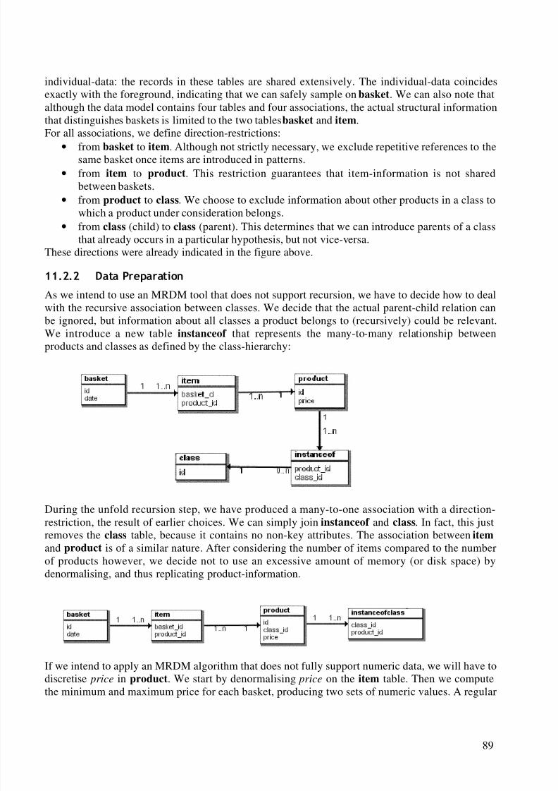
8/8/2019 Knobbe a.J. Multi-Relational Data Mining
http://slidepdf.com/reader/full/knobbe-aj-multi-relational-data-mining 100/129
89
individual-data: the records in these tables are shared extensively. The individual-data coincidesexactly with the foreground, indicating that we can safely sample on basket. We can also note thatalthough the data model contains four tables and four associations, the actual structural informationthat distinguishes baskets is limited to the two tables basket and item.
For all associations, we define direction-restrictions:• from basket to item. Although not strictly necessary, we exclude repetitive references to thesame basket once items are introduced in patterns.
• from item to product. This restriction guarantees that item-information is not sharedbetween baskets.
• from product to class. We choose to exclude information about other products in a class towhich a product under consideration belongs.
• from class (child) to class (parent). This determines that we can introduce parents of a classthat already occurs in a particular hypothesis, but not vice-versa.
These directions were already indicated in the figure above.
'DWD3UHSDUDWLRQAs we intend to use an MRDM tool that does not support recursion, we have to decide how to dealwith the recursive association between classes. We decide that the actual parent-child relation canbe ignored, but information about all classes a product belongs to (recursively) could be relevant.We introduce a new table instanceof that represents the many-to-many relationship betweenproducts and classes as defined by the class-hierarchy:
During the unfold recursion step, we have produced a many-to-one association with a direction-restriction, the result of earlier choices. We can simply join instanceof and class. In fact, this justremoves the class table, because it contains no non-key attributes. The association between item
and product is of a similar nature. After considering the number of items compared to the numberof products however, we decide not to use an excessive amount of memory (or disk space) bydenormalising, and thus replicating product-information.
If we intend to apply an MRDM algorithm that does not fully support numeric data, we will have todiscretise price in product. We start by denormalising price on the item table. Then we compute
the minimum and maximum price for each basket, producing two sets of numeric values. A regular
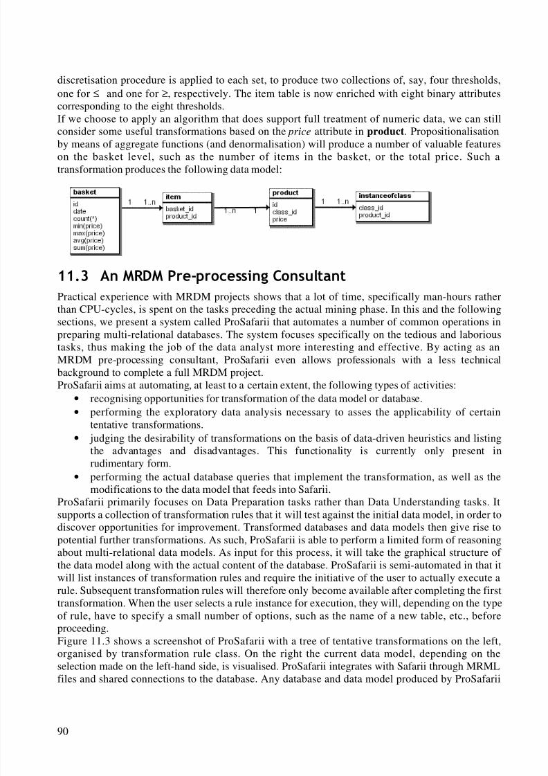
8/8/2019 Knobbe a.J. Multi-Relational Data Mining
http://slidepdf.com/reader/full/knobbe-aj-multi-relational-data-mining 101/129
90
discretisation procedure is applied to each set, to produce two collections of, say, four thresholds,one for ≤ and one for ≥, respectively. The item table is now enriched with eight binary attributescorresponding to the eight thresholds.If we choose to apply an algorithm that does support full treatment of numeric data, we can still
consider some useful transformations based on the price attribute in product. Propositionalisationby means of aggregate functions (and denormalisation) will produce a number of valuable featureson the basket level, such as the number of items in the basket, or the total price. Such atransformation produces the following data model:
$Q05'03UHSURFHVVLQJ&RQVXOWDQWPractical experience with MRDM projects shows that a lot of time, specifically man-hours ratherthan CPU-cycles, is spent on the tasks preceding the actual mining phase. In this and the followingsections, we present a system called ProSafarii that automates a number of common operations inpreparing multi-relational databases. The system focuses specifically on the tedious and laborioustasks, thus making the job of the data analyst more interesting and effective. By acting as anMRDM pre-processing consultant, ProSafarii even allows professionals with a less technicalbackground to complete a full MRDM project.ProSafarii aims at automating, at least to a certain extent, the following types of activities:
• recognising opportunities for transformation of the data model or database.
• performing the exploratory data analysis necessary to asses the applicability of certaintentative transformations.
• judging the desirability of transformations on the basis of data-driven heuristics and listingthe advantages and disadvantages. This functionality is currently only present inrudimentary form.
• performing the actual database queries that implement the transformation, as well as themodifications to the data model that feeds into Safarii.
ProSafarii primarily focuses on Data Preparation tasks rather than Data Understanding tasks. Itsupports a collection of transformation rules that it will test against the initial data model, in order todiscover opportunities for improvement. Transformed databases and data models then give rise to
potential further transformations. As such, ProSafarii is able to perform a limited form of reasoningabout multi-relational data models. As input for this process, it will take the graphical structure of the data model along with the actual content of the database. ProSafarii is semi-automated in that itwill list instances of transformation rules and require the initiative of the user to actually execute arule. Subsequent transformation rules will therefore only become available after completing the firsttransformation. When the user selects a rule instance for execution, they will, depending on the typeof rule, have to specify a small number of options, such as the name of a new table, etc., beforeproceeding.Figure 11.3 shows a screenshot of ProSafarii with a tree of tentative transformations on the left,organised by transformation rule class. On the right the current data model, depending on theselection made on the left-hand side, is visualised. ProSafarii integrates with Safarii through MRML
files and shared connections to the database. Any database and data model produced by ProSafarii
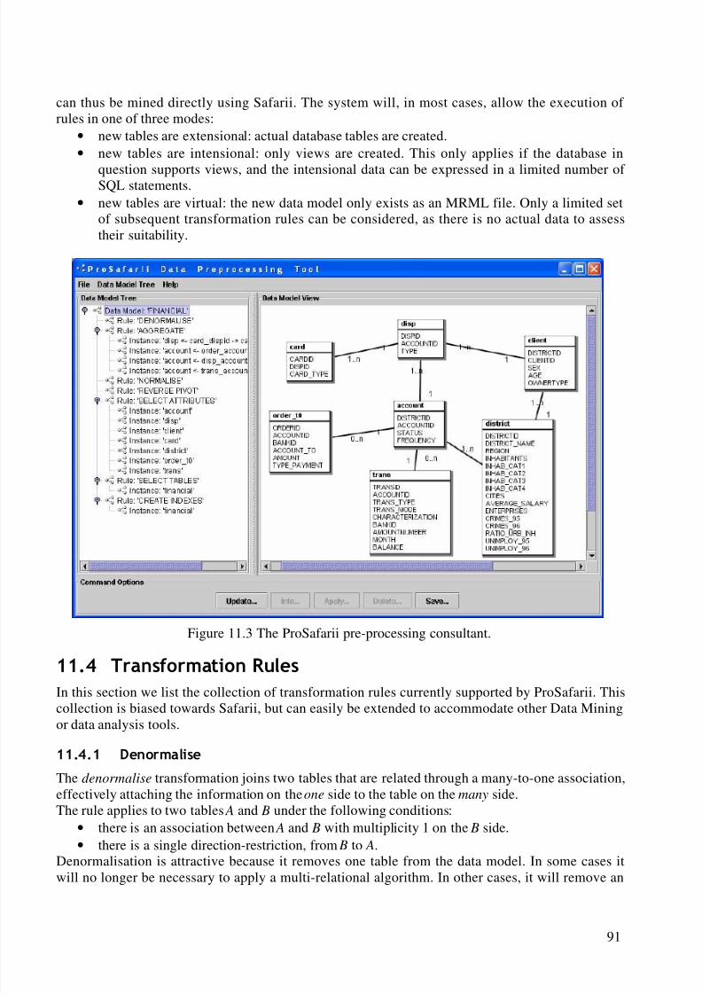
8/8/2019 Knobbe a.J. Multi-Relational Data Mining
http://slidepdf.com/reader/full/knobbe-aj-multi-relational-data-mining 102/129
91
can thus be mined directly using Safarii. The system will, in most cases, allow the execution of rules in one of three modes:
• new tables are extensional: actual database tables are created.• new tables are intensional: only views are created. This only applies if the database in
question supports views, and the intensional data can be expressed in a limited number of SQL statements.• new tables are virtual: the new data model only exists as an MRML file. Only a limited set
of subsequent transformation rules can be considered, as there is no actual data to assesstheir suitability.
Figure 11.3 The ProSafarii pre-processing consultant.
7UDQVIRUPDWLRQ5XOHV
In this section we list the collection of transformation rules currently supported by ProSafarii. Thiscollection is biased towards Safarii, but can easily be extended to accommodate other Data Miningor data analysis tools.
'HQRUPDOLVH
The denormalise transformation joins two tables that are related through a many-to-one association,effectively attaching the information on the one side to the table on the many side.The rule applies to two tables A and B under the following conditions:
• there is an association between A and B with multiplicity 1 on the B side.• there is a single direction-restriction, from B to A.
Denormalisation is attractive because it removes one table from the data model. In some cases itwill no longer be necessary to apply a multi-relational algorithm. In other cases, it will remove an
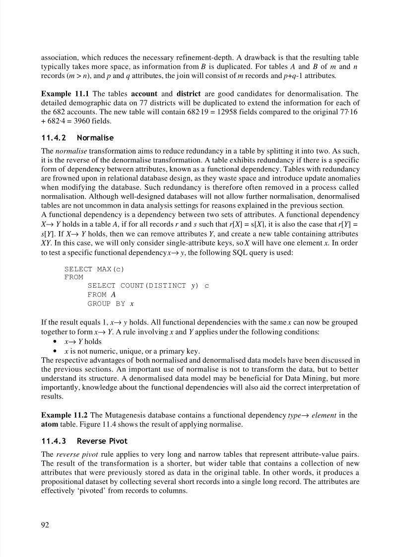
8/8/2019 Knobbe a.J. Multi-Relational Data Mining
http://slidepdf.com/reader/full/knobbe-aj-multi-relational-data-mining 103/129
92
association, which reduces the necessary refinement-depth. A drawback is that the resulting tabletypically takes more space, as information from B is duplicated. For tables A and B of m and n
records (m > n), and p and q attributes, the join will consist of m records and p+q-1 attributes.
Example 11.1 The tables account and district are good candidates for denormalisation. Thedetailed demographic data on 77 districts will be duplicated to extend the information for each of the 682 accounts. The new table will contain 682Â19 = 12958 fields compared to the original 77Â16+ 682Â4 = 3960 fields.
1RUPDOLVH
The normalise transformation aims to reduce redundancy in a table by splitting it into two. As such,it is the reverse of the denormalise transformation. A table exhibits redundancy if there is a specificform of dependency between attributes, known as a functional dependency. Tables with redundancyare frowned upon in relational database design, as they waste space and introduce update anomalieswhen modifying the database. Such redundancy is therefore often removed in a process called
normalisation. Although well-designed databases will not allow further normalisation, denormalisedtables are not uncommon in data analysis settings for reasons explained in the previous section.A functional dependency is a dependency between two sets of attributes. A functional dependency X → Y holds in a table A, if for all records r and s such that r [ X ] = s[ X ], it is also the case that r [Y ] =s[Y ]. If X → Y holds, then we can remove attributes Y , and create a new table containing attributes XY . In this case, we will only consider single-attribute keys, so X will have one element x. In orderto test a specific functional dependency x→ y, the following SQL query is used:
SELECT MAX(c)FROM
SELECT COUNT(DISTINCT y) c
FROM AGROUP BY x
If the result equals 1, x→ y holds. All functional dependencies with the same x can now be groupedtogether to form x→ Y . A rule involving x and Y applies under the following conditions:
• x→ Y holds• x is not numeric, unique, or a primary key.
The respective advantages of both normalised and denormalised data models have been discussed inthe previous sections. An important use of normalise is not to transform the data, but to betterunderstand its structure. A denormalised data model may be beneficial for Data Mining, but more
importantly, knowledge about the functional dependencies will also aid the correct interpretation of results.
Example 11.2 The Mutagenesis database contains a functional dependency type→ element in theatom table. Figure 11.4 shows the result of applying normalise.
5HYHUVH3LYRW
The reverse pivot rule applies to very long and narrow tables that represent attribute-value pairs.The result of the transformation is a shorter, but wider table that contains a collection of newattributes that were previously stored as data in the original table. In other words, it produces apropositional dataset by collecting several short records into a single long record. The attributes are
effectively ‘pivoted’ from records to columns.
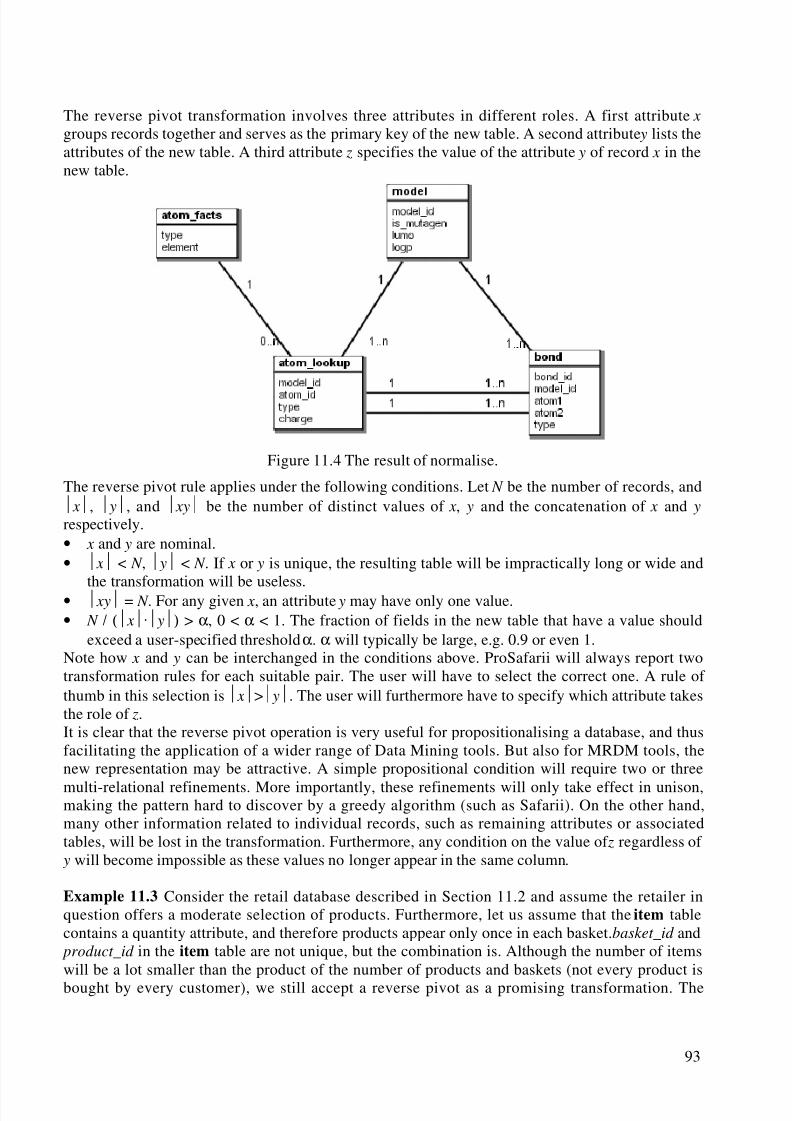
8/8/2019 Knobbe a.J. Multi-Relational Data Mining
http://slidepdf.com/reader/full/knobbe-aj-multi-relational-data-mining 104/129
93
The reverse pivot transformation involves three attributes in different roles. A first attribute x
groups records together and serves as the primary key of the new table. A second attribute y lists theattributes of the new table. A third attribute z specifies the value of the attribute y of record x in thenew table.
Figure 11.4 The result of normalise.
The reverse pivot rule applies under the following conditions. Let N be the number of records, and⏐ x⏐, ⏐ y⏐, and ⏐ xy⏐ be the number of distinct values of x, y and the concatenation of x and y
respectively.• x and y are nominal.• ⏐ x⏐ < N , ⏐ y⏐ < N . If x or y is unique, the resulting table will be impractically long or wide and
the transformation will be useless.• ⏐ xy⏐ = N . For any given x, an attribute y may have only one value.• N / (⏐ x⏐Â⏐ y⏐) > α, 0 < α < 1. The fraction of fields in the new table that have a value should
exceed a user-specified threshold α. α will typically be large, e.g. 0.9 or even 1.Note how x and y can be interchanged in the conditions above. ProSafarii will always report twotransformation rules for each suitable pair. The user will have to select the correct one. A rule of thumb in this selection is ⏐ x⏐>⏐ y⏐. The user will furthermore have to specify which attribute takesthe role of z.It is clear that the reverse pivot operation is very useful for propositionalising a database, and thusfacilitating the application of a wider range of Data Mining tools. But also for MRDM tools, thenew representation may be attractive. A simple propositional condition will require two or three
multi-relational refinements. More importantly, these refinements will only take effect in unison,making the pattern hard to discover by a greedy algorithm (such as Safarii). On the other hand,many other information related to individual records, such as remaining attributes or associatedtables, will be lost in the transformation. Furthermore, any condition on the value of z regardless of y will become impossible as these values no longer appear in the same column.
Example 11.3 Consider the retail database described in Section 11.2 and assume the retailer inquestion offers a moderate selection of products. Furthermore, let us assume that the item tablecontains a quantity attribute, and therefore products appear only once in each basket. basket_id and product_id in the item table are not unique, but the combination is. Although the number of itemswill be a lot smaller than the product of the number of products and baskets (not every product isbought by every customer), we still accept a reverse pivot as a promising transformation. The
8/8/2019 Knobbe a.J. Multi-Relational Data Mining
http://slidepdf.com/reader/full/knobbe-aj-multi-relational-data-mining 105/129
94
resulting table contains basket_id , as well as attributes for each product. Each field represents thequantity of a product in a particular basket. Although the other tables are still available, we couldmake the new table the target and analyse it with a propositional algorithm, e.g. Apriori [5]. Thenew table does not however allow us to work in multi-relational style, and use background
knowledge from product and class, or query the quantity of items regardless of their product code.Clearly, the resulting table only serves a special purpose, that is being the input to limitedalgorithms such as Apriori.
$JJUHJDWH
The aggregate transformation involves the aggregation step, as described in Chapter 7. Thistransformation enriches the information in one table with aggregated information from anothertable, joined by a one-to-many association. This second table is left unaltered. The rule applies totwo tables A and B under the following conditions:• there is an association between A and B with multiplicity 1 on the A side, and 0..n or 1..n on the
B side.
• There is at least one non-key attribute in B.As was demonstrated in Chapter 8 and 9, aggregate functions can be a very powerful tool to capturelocal structure. Because the aggregate transformation preserves the original table, it improves theinformation available to MRDM algorithms. As Chapter 8 demonstrates, repeated aggregation mayproduce a flat table fit for analysis using traditional tools. The only downside to this transformationis the increased space required.
Example 11.4 Figure 11.5 shows the result of four aggregate rules applied to the Mutagenesisdatabase. Information from atom and bond is aggregated at molecule, and bond is aggregatedtwice at atom, once for each association. The appropriate set of aggregate functions depends on thedata type of the attributes.
6HOHFW$WWULEXWHV
The select attributes transformation performs an obvious, yet practical and common operation:produce a table that contains a subset of the attributes of the original table. The rule applies to anytable that has one or more non-key attributes. Clearly this rule depends entirely on input from theuser.
6HOHFWWDEOHV
The select tables transformation provides a basic service: it removes tables from the data model (butnot from the database) as indicated by the user.
&UHDWH,QGH[HV
The create indexes transformation does not change anything in the data model or in the underlyingdata, and is therefore not strictly a pre-processing operation. It is however, a very useful operationbefore any MRDM run, as it will improve the performance of the RDBMS on data miningprimitives. The transformation will create database indexes for the primary and foreign key relatedto each association in the data model. The data structure that each index represents will speed upany joins performed over the association. The tedious task of considering the structure of thedatabase, and subsequently creating the necessary indexes is thus automated by ProSafarii.
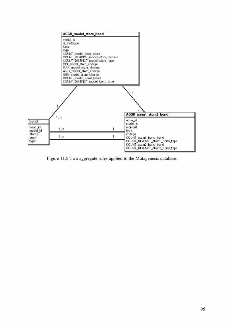
8/8/2019 Knobbe a.J. Multi-Relational Data Mining
http://slidepdf.com/reader/full/knobbe-aj-multi-relational-data-mining 106/129
95
Figure 11.5 Two aggregate rules applied to the Mutagenesis database.

8/8/2019 Knobbe a.J. Multi-Relational Data Mining
http://slidepdf.com/reader/full/knobbe-aj-multi-relational-data-mining 107/129
This page intentionally left blank
8/8/2019 Knobbe a.J. Multi-Relational Data Mining
http://slidepdf.com/reader/full/knobbe-aj-multi-relational-data-mining 108/129
97
&RQFOXVLRQ
&RQWULEXWLRQV
In this section we outline the main contributions of this thesis.We have defined Structured Data Mining as the genus of Data Mining paradigms concerned with
structured data. SDM provides a unified framework for important concepts shared by the differentparadigms. We have shown how, and to what extent four popular SDM approaches implement theseconcepts, and in what areas each of these paradigms excels. Specifically, we have outlined Multi-Relational Data Mining, a paradigm that is concerned with structured data in relational form.We have demonstrated how structured individuals can be described by features based on localstructure. Such features fall into two classes: existential features, which express the presence of specific substructures, and aggregate functions, which express global properties of groups of parts.Three pattern languages (with increasing expressive power) have been defined that can be used toselect individuals, or define subgroups. Selection graphs can be used to select individuals purely onthe basis of existential features. Extended selection graphs also work with existential features, butadd the possibility of complementary patterns, a necessity for Divide-and-Conquer approaches.Finally, generalised selection graphs offer the possibility of aggregate functions, combined withexistential features.An important aspect of our MRDM framework is declarative bias. Relational databases aregenerally well-designed, and the underlying data model is an important means of guiding the searchfor patterns and achieving efficiency. We have introduced the popular Unified Modeling Language(UML) as declarative bias language in MRDM. The UML data model that describes the structure of the database both acts as a restriction on the shape of individuals, as well as on that of tentativemodels of the data. For Data Mining software to work with the graphical data models in UML, wehave defined an XML dialect called MRML (Multi-Relational Modelling Language) that representsthe same information serially.
In order to support the analysis of industrial-size databases stored in an RDBMS, we have outlineda Client/Server architecture that organises the major computational processes in data analysis. This
8/8/2019 Knobbe a.J. Multi-Relational Data Mining
http://slidepdf.com/reader/full/knobbe-aj-multi-relational-data-mining 109/129
98
architecture revolves around a set of multi-relational data mining primitives that each support one of the refinement steps within the different pattern languages. The primitives are a means of separatingthe data access challenge from the actual pattern discovery. The information contained in such aprimitive is both sufficient for the algorithm to guide the search, as well as (relatively) easy to
compute for the query processing component of the architecture (typically the RDBMS).We have defined four algorithms for analysing multi-relational data. Three of these algorithms workwith one of the above-mentioned pattern languages in turn. A fourth algorithm involves pre-processing of the data in order to arrive at a representation that is suitable for existing propositionalalgorithms. A comparison of these four algorithms is given in Section 12.3. The Multi-RelationalRule Discovery algorithm that works with selection graphs has been the basis of a commercialMRDM tool, called Safarii. This systems is based on the presented architecture.The MRDM technology presented in this thesis mainly pertains to the modelling step of a largerprocess, which is often referred to as Knowledge Discovery in Databases (KDD) [33]. As werecognise the importance of the remaining steps in this process, we have presented an MRDMproject blueprint. This blueprint outlines how we can arrive at a dataset that is suitable for mining.
The blueprint focuses on two major tasks, Data Understanding and Data Preparation. The first taskis concerned with deciding the best way to approach an analysis task on the basis of available meta-data describing the database. The second task deals with pre-processing the data in a way thatemphasises promising features of the individuals, and that is optimal for the mining algorithm of choice.In order to support the data analyst in these activities, we have developed an MRDM pre-processingconsultant. The application, called ProSafarii, makes a superficial scan of the data model and theactual database, and suggests a number of interesting transformations of the database. Each of thesetransformations potentially allows a number of further transformations. After validation by the user,the system performs selected transformations by executing the necessary queries in the RDBMS. Itfurthermore updates the data model to enable direct analysis of the derived database by MRDM
tools such as Safarii. As a by-product of the transformations that are found to be applicable, thesystem provides a basic degree of insight into the structure of the data model.
9DOLGLW\RI05'0$SSURDFK
This thesis deals with Multi-Relational Data Mining. From the start we have defined our MRDMapproach as one of a collection of Structured Data Mining paradigms. Although based on differentrepresentational settings, these paradigms are very similar in their treatment of structured data. Sohas our emphasis on MRDM been justified, or have we just reformulated achievements of SDMparadigms with a longer history, such as ILP?One of our motivations for considering MRDM in detail was to benefit from a large body of
research in the field of relational databases, for example where data modelling, query languages andquery optimisation is concerned. The intended ‘paradigm shift’ would inspire new developments inSDM that seem logical steps in a multi-relational setting, but may have been overlooked inalternative paradigms. A certain degree of reinventing the wheel is a necessary element of ourwhish to take a fresh look at the analysis of structured data. Still, we can outline a number of important developments that validate MRDM as a strong competitor to alternative SDM paradigms.The validity of MRDM is further supported by empirical results as described in the differentsections on experimental evaluation. We mention a number of areas where MRDM outperformsrelated paradigms.First, there is the strong role of the data model of the database as declarative bias for the searchprocess. Rather than trying to define the shape of patterns the algorithm is required to discover,
MRDM uses the structure of the database in UML to guide the search. The same data model is used
8/8/2019 Knobbe a.J. Multi-Relational Data Mining
http://slidepdf.com/reader/full/knobbe-aj-multi-relational-data-mining 110/129
99
in transformation-based approaches such as propositionalisation or semi-automated pre-processing(see Section 11.3). A similar database orientation inspires a further strong point of MRDM:hypothesis testing in the RDBMS. The Client/Server architecture that separates the miningalgorithms from the data handling offers a range of opportunities for query optimisations (e.g.
parallelisation, batch processing) independent of the actual mining algorithm. The proposed DataMining primitives already achieve an initial level of optimisation by combining several hypothesesinto one query.A further characteristic of MRDM is its incorporation of aggregate functions in pattern languages.Different experiments show that such features can be very powerful, particularly in the presence of numeric data and high levels of non-determinacy. Although existential features are a logical choicein certain SDM paradigms, for example first-order logic in ILP or subgraphs in GM, they are simplytoo restrictive in a range of application domains.Although not entirely exclusive to MRDM, the full treatment of numeric data seems to be typicalfor this paradigm. This subject has often been ignored because it conflicts with a number of popularconcepts, such as exhaustive search or frequent pattern discovery. Still, empirical comparisons
show that SDM algorithms benefit from good support for numeric data. See for example Chapter 6,or [69, 85].These qualities of MRDM clearly show that our emphasis on this field has paid off, and in factMRDM deserves further attention in the future. However, the choice of paradigm to employ whendealing with structured data will in practice be a question of taste. Because the different paradigmshave a lot in common, people are likely to base their choice on ‘superficial’ properties, such asthose outlined in Table 2.1.
2YHUYLHZRI$OJRULWKPV
In this thesis we have presented four algorithms that approach the analysis of multi-relational data
in a variety of ways. Although it is often wise to approach a problem from multiple sides, and trymore than one algorithm, one could wonder which of these four algorithms is the preferred choicefor a given MRDM problem. In this section we will shed some light on the particulars of eachalgorithm.The most important feature of a problem that influences the choice of algorithm is whether the taskis predictive or descriptive in nature. If the task is predictive, one is interested in global models thatgive a unique classification of each individual, be it an individual that occurs in the database at handor in as yet unseen databases. Predictive models are primarily aimed at classifying unseenindividuals for which the target value is unknown. A descriptive data Mining task on the other handis concerned with producing local models that explain particular aspects of the data, or uncoverpartial dependencies. As such, the aim is possibly fragmented but increased understanding, rather
than a full explanation that is geared towards prediction. The algorithms SGRules and GSGRulesare descriptive. MRDTL (as an instance of our decision tree induction framework) and RollUp +C5.0 (as an instance of Polka) are predictive. Note that the predictive nature of this last algorithm isthe result of using C5.0. RollUp can be employed in a descriptive fashion, given the rightpropositional algorithm.RollUp and GSGRules both include aggregate functions. As we have seen, aggregate functions area potentially richer means of capturing local structure compared to existential features only. Section9.3 demonstrates in practice the increased descriptive power of GSGRules compared to SGRules.However, this power comes at the price of lower efficiency or a smaller proportion of the searchspace being considered. Furthermore, patterns that include aggregate functions can be more difficultto interpret.
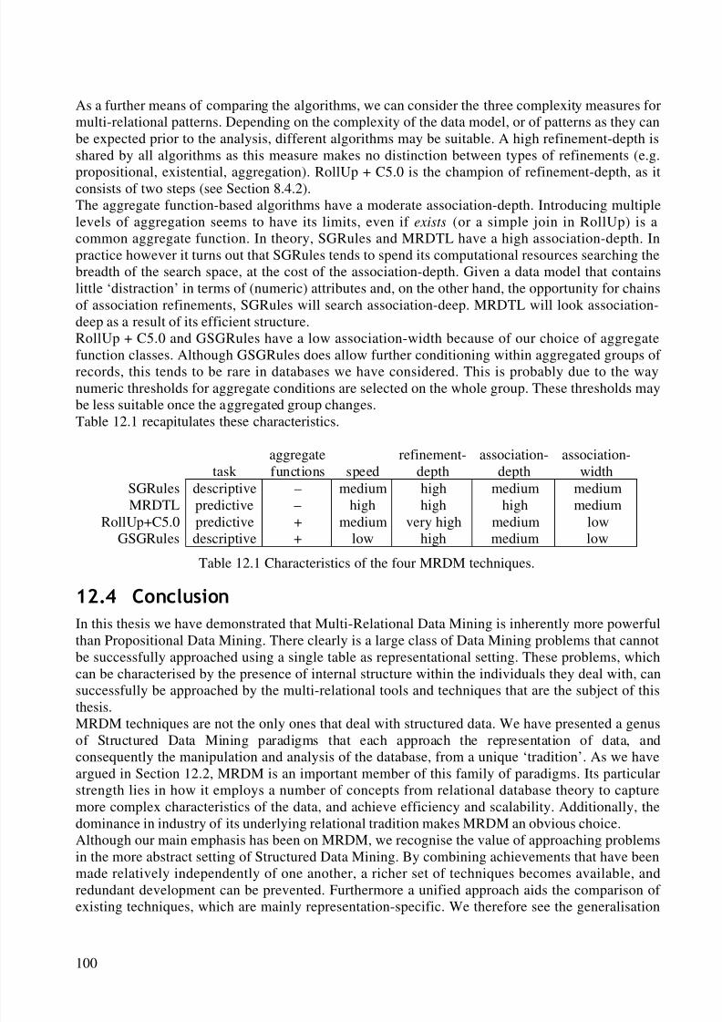
8/8/2019 Knobbe a.J. Multi-Relational Data Mining
http://slidepdf.com/reader/full/knobbe-aj-multi-relational-data-mining 111/129
100
As a further means of comparing the algorithms, we can consider the three complexity measures formulti-relational patterns. Depending on the complexity of the data model, or of patterns as they canbe expected prior to the analysis, different algorithms may be suitable. A high refinement-depth isshared by all algorithms as this measure makes no distinction between types of refinements (e.g.
propositional, existential, aggregation). RollUp + C5.0 is the champion of refinement-depth, as itconsists of two steps (see Section 8.4.2).The aggregate function-based algorithms have a moderate association-depth. Introducing multiplelevels of aggregation seems to have its limits, even if exists (or a simple join in RollUp) is acommon aggregate function. In theory, SGRules and MRDTL have a high association-depth. Inpractice however it turns out that SGRules tends to spend its computational resources searching thebreadth of the search space, at the cost of the association-depth. Given a data model that containslittle ‘distraction’ in terms of (numeric) attributes and, on the other hand, the opportunity for chainsof association refinements, SGRules will search association-deep. MRDTL will look association-deep as a result of its efficient structure.RollUp + C5.0 and GSGRules have a low association-width because of our choice of aggregate
function classes. Although GSGRules does allow further conditioning within aggregated groups of records, this tends to be rare in databases we have considered. This is probably due to the waynumeric thresholds for aggregate conditions are selected on the whole group. These thresholds maybe less suitable once the aggregated group changes.Table 12.1 recapitulates these characteristics.
taskaggregatefunctions speed
refinement-depth
association-depth
association-width
SGRules descriptive – medium high medium mediumMRDTL predictive – high high high medium
RollUp+C5.0 predictive + medium very high medium low
GSGRules descriptive + low high medium lowTable 12.1 Characteristics of the four MRDM techniques.
&RQFOXVLRQ
In this thesis we have demonstrated that Multi-Relational Data Mining is inherently more powerfulthan Propositional Data Mining. There clearly is a large class of Data Mining problems that cannotbe successfully approached using a single table as representational setting. These problems, whichcan be characterised by the presence of internal structure within the individuals they deal with, cansuccessfully be approached by the multi-relational tools and techniques that are the subject of thisthesis.MRDM techniques are not the only ones that deal with structured data. We have presented a genusof Structured Data Mining paradigms that each approach the representation of data, andconsequently the manipulation and analysis of the database, from a unique ‘tradition’. As we haveargued in Section 12.2, MRDM is an important member of this family of paradigms. Its particularstrength lies in how it employs a number of concepts from relational database theory to capturemore complex characteristics of the data, and achieve efficiency and scalability. Additionally, thedominance in industry of its underlying relational tradition makes MRDM an obvious choice.Although our main emphasis has been on MRDM, we recognise the value of approaching problemsin the more abstract setting of Structured Data Mining. By combining achievements that have beenmade relatively independently of one another, a richer set of techniques becomes available, and
redundant development can be prevented. Furthermore a unified approach aids the comparison of existing techniques, which are mainly representation-specific. We therefore see the generalisation
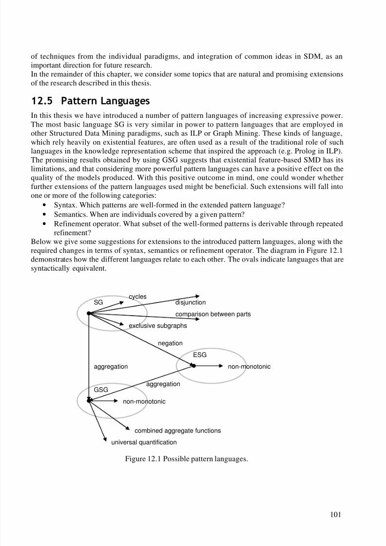
8/8/2019 Knobbe a.J. Multi-Relational Data Mining
http://slidepdf.com/reader/full/knobbe-aj-multi-relational-data-mining 112/129
101
of techniques from the individual paradigms, and integration of common ideas in SDM, as animportant direction for future research.In the remainder of this chapter, we consider some topics that are natural and promising extensionsof the research described in this thesis.
3DWWHUQ/DQJXDJHV
In this thesis we have introduced a number of pattern languages of increasing expressive power.The most basic language SG is very similar in power to pattern languages that are employed inother Structured Data Mining paradigms, such as ILP or Graph Mining. These kinds of language,which rely heavily on existential features, are often used as a result of the traditional role of suchlanguages in the knowledge representation scheme that inspired the approach (e.g. Prolog in ILP).The promising results obtained by using GSG suggests that existential feature-based SMD has itslimitations, and that considering more powerful pattern languages can have a positive effect on thequality of the models produced. With this positive outcome in mind, one could wonder whetherfurther extensions of the pattern languages used might be beneficial. Such extensions will fall intoone or more of the following categories:
• Syntax. Which patterns are well-formed in the extended pattern language?• Semantics. When are individuals covered by a given pattern?• Refinement operator. What subset of the well-formed patterns is derivable through repeated
refinement?Below we give some suggestions for extensions to the introduced pattern languages, along with therequired changes in terms of syntax, semantics or refinement operator. The diagram in Figure 12.1demonstrates how the different languages relate to each other. The ovals indicate languages that aresyntactically equivalent.
Figure 12.1 Possible pattern languages.
SG disjunction
comparison between parts
GSG
ESG
cycles
exclusive subgraphs
non-monotonic
negation
aggregation
universal quantification
combined aggregate functions
aggregation
non-monotonic
8/8/2019 Knobbe a.J. Multi-Relational Data Mining
http://slidepdf.com/reader/full/knobbe-aj-multi-relational-data-mining 113/129
102
• Allow cycles in the selection graphs. This can be achieved by a simple addition to thenormal refinement operator that adds edges between two existing nodes in the graph. Thefollowing pattern is an example:
‘the set of molecules that contain two atoms joined by a bond’• Interpret subgraphs of a particular node connected by the same association as referring to
distinct parts in the individual. Such an extension deals with the semantics of SG. Selectiongraphs that appear as usual now select different subgroups.
‘the set of molecules that contain a C-atom and a different atom of charge greaterthan 6.60Â10-7’
• Allow disjunctive conditions in selection nodes. The current set of conditions associatedwith each node represents a conjunction of conditions, whereas both the syntax and the
semantics could be changed in order to incorporate both. Note that disjunction will introducenon-monotonic refinements.
‘the set of molecules that contain a Br, Cl, F, or I-atom’
This example covers 22 individuals in the Mutagenesis database and has a novelty of –0.030 (see also Section 5.2).
• Allow comparison between selection nodes of the same class, for example, between twoinstances of the same attribute. Previously, comparison between parts was exclusive to theconcept of associations. A less restrictive notion can be used to allow the comparison of attributes of parts other than the primary and foreign keys.
‘the set of molecules that contain 2 atoms of equal element’
• Include non-monotonic refinements in ESG. Adding conditions to absent subgraphsintroduces a generalisation and is thus not acceptable in top-down algorithms such aspresented in Chapter 6. Interesting patterns can however be considered if non-monotonicsearch is allowed.
‘the set of molecules that do not contain an O-atom’
• Include non-monotonic refinements in GSG.
‘the set of molecules that contain at most 5 C-atoms’
• Include universal quantification over associations: every part that is introduced over anassociation should meet the specified conditions. Because universal quantification captureslocal structure, one can think of it as a special type of aggregate condition, although theinteraction between aggregate function and further conditions is different. Conditions on thesubgraphs should not be interpreted as selections on the sets of parts that are aggregated, butrather as necessary features of all parts.
8/8/2019 Knobbe a.J. Multi-Relational Data Mining
http://slidepdf.com/reader/full/knobbe-aj-multi-relational-data-mining 114/129
103
‘the set of molecules that contain just C-atoms’
• Include nested aggregate functions that work over multiple associations. The virtual attributecreated by the first aggregate function is the argument of a second function, and so on. This
kind of nested aggregate function is produced by the pre-processing procedure Roll-Up, buta more general dynamic algorithm based on extensions of GSG does not exist.
‘the set of molecules that have an average bond-count per atom greater than 2.6’
• Include aggregate functions over a single association that are arithmetic functions of thebasic set of aggregate function classes used thus far (count, min, max, etc.).
‘the set of molecules that have a difference between the minimum and maximumatom-charge less than 4.37Â10-5’
The list of flavours of the features to extract from structured data is long, and seemingly tempting.The expressive power of each of these extensions may be of benefit to upgraded Data Miningalgorithms. Even if technical difficulties to implement these algorithms can be overcome, theincreased expressiveness comes at a substantial price. One could wonder how transparent orunderstandable less trivial variations of the example patterns mentioned above are to human users.Also, the new constructs will increase the level of redundancy in the output (as well as in candidatequeues), and leave room for many logically equivalent or at least very similar rules.A more important consideration is the effect of such extensions on the size of the hypothesis space.Practical and user-friendly Data Mining systems will be allowed a fixed amount of time or numberof hypotheses to test. Any increase in size of the hypothesis space will hence result in a smallerfraction actually being considered. As a consequence, good patterns may be overlooked. Although a
bigger and richer hypothesis space holds the promise of better patterns, the chances of actuallydiscovering such patterns will decrease. In our view, we have already reached the limit in thisrespect with the current implementation of rule induction in GSG.Still, a number of the suggested patterns appear as natural as the kind of patterns that is consideredby current MDRM algorithms. Specifically, the patterns that cannot be reached by top-down searchdeserve attention, albeit maybe in a restricted form. Before richer pattern languages can beconsidered however, the fairly straightforward search strategies presented in the previous chaptersneed to be refined, in order to explore the larger search space effectively. In the following section,we consider a number of necessary improvements in multi-relational search.
,PSURYHG6HDUFKThe search strategies employed in the Rule Discovery algorithms in this thesis are fairlystraightforward. As a result, these algorithms may suffer from some effects that will become moreimportant with enrichments of the pattern languages as suggested in the previous section. In order tocontinue to be able to effectively and efficiently consider a promising subset of hypotheses, theseundesirable issues must be addressed.The most obvious problem is poor efficiency due to a large number of hypotheses being tested onthe database. An important reduction in the data mining primitives executed can be achieved byremoving redundant hypotheses. The current refinement operators (as defined in Chapter 4, 6 and 9)will sometimes produce the same selection graph multiple times as a result of alternative orderingsof refinements. The solution is to use an optimal refinement operator: every point in the searchspace can only be reached along a single path of refinements. This optimality is typically achieved
8/8/2019 Knobbe a.J. Multi-Relational Data Mining
http://slidepdf.com/reader/full/knobbe-aj-multi-relational-data-mining 115/129
104
by defining an ordering on refinements through lexicographic comparison. Unfortunately, thissyntactic notion of optimality only works in combination with exhaustive search. It conflicts withthe heuristic search strategies that are vital in larger industrial applications. Different classes of heuristics may choose refinement paths that are prohibited by the optimal refinement operator.
A more pragmatic approach to avoiding redundant hypothesis testing is to maintain a data structureof previously considered patterns, and check for redundancy before testing on the database. Thismethod has attained some popularity in Propositional Data Mining due to the availability of efficient indexing structures for retrieving equivalent or otherwise relevant previous hypotheses.The trade-off between executing a database query and searching in the data structure has thus beenin favour of the latter. In Structured Data Mining, such indexing of patterns is less trivial and moreresearch is required to produce data structures that justify the effort.Another important method of reducing hypothesis testing is known as optimistic estimate pruning.This method is applied for example in the ILP-systems MIDOS [31, 107] and Tertius [36]. It relieson the idea that it is possible to estimate the score of the best pattern that can ever be derived fromthe pattern at hand, keeping in mind that there is a limit to the amount of change in distribution in
the subgroups resulting from the minimum coverage constraint. If this optimistic estimate is worsethan the score of the current pattern or its ancestors, or worse than the minimum score, then theentire subtree of the search space can be pruned. Optimistic estimates can be derived for all of thepopular rule measures. These estimate functions typically consider the ‘ideal’ pattern, for exampleone that covers all the positive examples, and compute its score.The important challenge in richer pattern languages deals with non-monotonic refinement operators.Such operators are refinement operators that are not specialisation operators: refined patterns do notnecessarily produce subsets of the original subgroup. This property makes top-down searchimpossible. In itself this need not be a problem. Exhaustive search of a particular hypothesis spacedefined by a maximum pattern complexity (i.e. refinement depth) can be done in any order. Inpractical cases however, exhaustive search is unrealistic, and some form of heuristic (parallel) hill-
climbing is required that relies heavily on monotonicity. So what are the effects of dispensing withmonotonicity? First of all, there is no pruning on minimum coverage. Although we can filter theultimate result on coverage, intermediate hypotheses along the refinement path may even have zerocoverage. An important source of efficiency is thus lost. Important Data Mining algorithms such asApriori [5] rely on minimum coverage pruning for their practical applicability. Secondly, theoptimistic estimate pruning mentioned above cannot be applied as it relies both on a minimumcoverage and on derived patterns being a subset of the current pattern. Finally, the heuristics used toguide the search (typically the score of the pattern at hand, or an optimistic estimate of its subtree)become problematic.The solution is to use a form of look-ahead in order to bridge intermediate hypotheses with a lowcoverage. A superficial form of such a look-ahead involves deriving a monotonic refinement
operator from a non-monotonic one by combining refinement steps. This can be achieved bypreceding every generalisation by a specialisation, such that the combined result is a specialisation.This combination of refinement steps is not unlike the look-ahead in multi-relational decision treeinduction. Unfortunately, this solution is limited as is excludes refinement paths that involvemultiple consecutive generalisations.
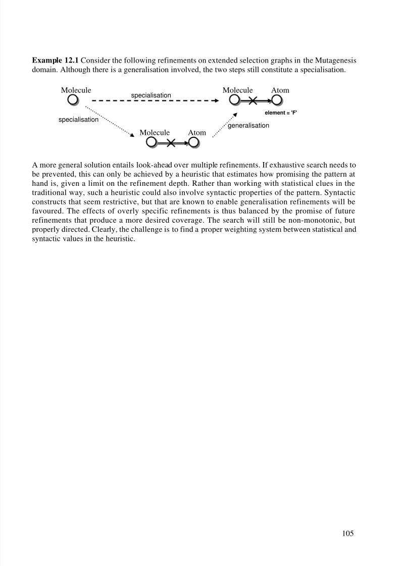
8/8/2019 Knobbe a.J. Multi-Relational Data Mining
http://slidepdf.com/reader/full/knobbe-aj-multi-relational-data-mining 116/129
105
Example 12.1 Consider the following refinements on extended selection graphs in the Mutagenesisdomain. Although there is a generalisation involved, the two steps still constitute a specialisation.
A more general solution entails look-ahead over multiple refinements. If exhaustive search needs tobe prevented, this can only be achieved by a heuristic that estimates how promising the pattern athand is, given a limit on the refinement depth. Rather than working with statistical clues in thetraditional way, such a heuristic could also involve syntactic properties of the pattern. Syntacticconstructs that seem restrictive, but that are known to enable generalisation refinements will befavoured. The effects of overly specific refinements is thus balanced by the promise of futurerefinements that produce a more desired coverage. The search will still be non-monotonic, butproperly directed. Clearly, the challenge is to find a proper weighting system between statistical andsyntactic values in the heuristic.
Molecule
generalisation
specialisation
specialisation
AtomMolecule
element = 'F'
AtomMolecule

8/8/2019 Knobbe a.J. Multi-Relational Data Mining
http://slidepdf.com/reader/full/knobbe-aj-multi-relational-data-mining 117/129
This page intentionally left blank
8/8/2019 Knobbe a.J. Multi-Relational Data Mining
http://slidepdf.com/reader/full/knobbe-aj-multi-relational-data-mining 118/129
107
$SSHQGL[$050/
The Document Type Definition (DTD) of the MRML file format is as follows:
<?xml version="1.0" encoding="UTF-8"?>
<!ELEMENT mrml (version, database, datamodel)>
<!ELEMENT database (name, server?, host?, user?, password?)><!ELEMENT datamodel (name, table+, association*)>
<!ELEMENT table (name, attribute+)>
<!ELEMENT attribute (name)>
<!ATTLIST attribute type (nominal|numeric|key|primarykey) #REQUIRED>
<!ATTLIST attribute id ID #IMPLIED>
<!ELEMENT association (name, keyref, keyref)>
<!ATTLIST association direction (none|forward|reverse|both) "forward">
<!ELEMENT keyref EMPTY>
<!ATTLIST keyref id IDREF #REQUIRED>
<!ATTLIST keyref multiplicity (zeroorone|one|zeroormore|oneormore) "zeroormore">
<!ELEMENT version (#PCDATA)>
<!ELEMENT server (#PCDATA)>
<!ELEMENT host (#PCDATA)>
<!ELEMENT user (#PCDATA)>
<!ELEMENT password (#PCDATA)>
<!ELEMENT name (#PCDATA)>
An MRML file describes in detail the data model of a database. Let us consider the majorcomponents in turn.
8/8/2019 Knobbe a.J. Multi-Relational Data Mining
http://slidepdf.com/reader/full/knobbe-aj-multi-relational-data-mining 119/129
108
<!ELEMENT database (name, server?, host?, user?, password?)>
This rule sates that the database element must contain a name of a physical database, andoptionally information concerning the location and access to the database.
<!ELEMENT datamodel (name, table+, association*)>
This states that a data model consists of at least one table, and zero or more associations.
<!ELEMENT table (name, attribute+)>
<!ELEMENT attribute (name)>
Every table element consists of at least one attribute that in turn consists of a name element.
<!ATTLIST attribute type (nominal|numeric|key|primarykey) #REQUIRED>
<!ATTLIST attribute id ID #IMPLIED>
The rules state that an attribute element contains one or two XML-attributes. An attribute atleast contains a type element, which indicates the nature of the data. The values nominal andnumeric refer to actual data, whereas key and primarykey indicate the use of this attribute inforeign key relations. The optional XML-attribute id is used to give a unique identifier forreference by other XML-elements.
<!ELEMENT association (name, keyref, keyref)>
<!ATTLIST association direction (none|forward|reverse|both) "forward">
An association element has a name and two references to keys. Furthermore theassociation has an XML-attribute direction, which specifies in which direction anassociation may be traversed.
<!ELEMENT keyref EMPTY>
<!ATTLIST keyref id IDREF #REQUIRED>
<!ATTLIST keyref multiplicity (zeroorone|one|zeroormore|oneormore) "zeroormore">
The keyref element contains one mandatory XML-attribute id that states the identifier of aparticular attribute in a table. An optional XML-attribute multiplicity fixes the multiplicity of the association in question (one on each side).
8/8/2019 Knobbe a.J. Multi-Relational Data Mining
http://slidepdf.com/reader/full/knobbe-aj-multi-relational-data-mining 120/129
%LEOLRJUDSK\
1. Abe, K., Kawasoe, S., Asai, T., Arimura, H., Arikawa, S. Optimized Substructure
Discovery for Semi-Structured Data, In Proceedings of PKDD 2002, LNAI 2431, 20022. Abiteboul, S., Buneman, P., and Suciu, D. Data on the Web, Morgan Kaufmann, 20003. Adriaans, P. Adaptive System Management , in Advances in Applied Ergonomics, In
Proceedings of ICAE'96, Istanbul, 19964. Adriaans, P., Zantinge, R. Data mining. Addison-Wesley, 19965. Agrawal, R., Mannila, H., Srikant, R., Toivonen, H., Verkamo, A. Fast Discovery of
Association Rules, in Artificial Intelligence, 19976. Alphonse, É., Rouveirol, C. Selective Propositionalization for Relational Learning, In
Proceedings of PKDD ’99, LNAI 1704, 19997. Appice, A., Ceci, M., Malerba, D. MR-SMOTI: A Data Mining System for Regression
Tasks Tightly-Coupled with a Relational Database, In Proceedings of KDID-2003, 20038. Asai, T., Abe, K., Kawasoe, S., Arimura, H., Sakamoto, H., and Arikawa, S. Efficient
substructure discovery from large semi-structured data, In Proceedings of SDM2002,
20029. Blockeel, H. Top-Down Induction of First Order Logical Decision Trees, Ph.D. thesis,1998
10. Blockeel, H., Dehaspe, L., Demoen, B., Janssens, G., Ramon, J., Vandecasteele, H.
Executing Query Packs in ILP, In Proceedings of ILP 2000, LNAI 1866, 200011. Blockeel, H., De Raedt, L. Relational knowledge discovery in databases, In Stephen
Muggleton, editor, In Proceedings of ILP '96, LNAI 314, pp. 199-211, 199612. Blockeel, H., De Raedt, L. Top-down induction of first order logical decision trees,
Artificial Intelligence, 101(1-2):285-297, June 199813. Blockeel, H., De Raedt, L., Jacobs, N., Demoen, B. Scaling up inductive logic
programming by learning from interpretations. Data Mining and knowledge Discovery,
3(1):59-93, March 1999
8/8/2019 Knobbe a.J. Multi-Relational Data Mining
http://slidepdf.com/reader/full/knobbe-aj-multi-relational-data-mining 121/129
110
14. Blockeel, H., De Raedt, L., Ramon, J. Top-down induction of clustering trees, InProceedings of ICML'98, 55-63, 1998
15. Boncz, P. Monet, a next-Generation DBMS Kernel for Query-Intensive Applications,Ph.D. thesis, 2002
16. Braga, D., Campi, A., Klemettinen, M., Lanzi, P. Mining Association Rules from XML Data, In Proceedings of DaWak 2002, 200217. Bray, T. Introduction to the Annotated XML Specification,
http://www.xml.com/axml/axml.html18. Chapman, P., Clinton, J., Khabaza, T., Reinartz, T., Wirth, R. The CRISP-DM Process
Model, 199919. Cook, D., Holder, L. Graph-Based Data Mining, Intelligent Systems & their
Applications, 15(2):32-41, 200020. Dasu, T., Johnson, T. Exploratory Data Mining and Data Cleaning, Wiley, 200321. Date, C. An Introduction to Database Systems, Volume I , The Systems Programming
Series, Addison-Wesley, 1986
22. Dehaspe, L. Frequent Pattern Discovery in First-Order Logic, Ph.D. thesis, 199823. Dehaspe, L., and De Raedt, L. Mining association rules in multiple relations, InProceedings of ILP’97, LNAI 1297, 1997
24. Dehaspe, L., Toivonen, H., Discovery of frequent Datalog patterns, Data Mining andKnowledge Discovery, 3(1), 1999
25. Dehaspe, L., Toivonen, H., King, R. Finding frequent substructures in chemical
compounds, In Proceedings of KDD '98, 30-36, 199826. Dewhurst, N., Lavington, S. Knowledge Discovery from Client/Server Databases, In
Proceedings of PKDD ’98, 199827. Dietterich, T., Lathrop, R., Lozano-Pérez, T. Solving the multiple-instance problem with
axis-parallel rectangles, Artificial Intelligence, 89(1-2):31-71, 1997
28. Džeroski, S. Inductive Logic Programming and Knowledge Discovery in Databases, in[33], AAAI Press, 1996
29. Džeroski, S., Blockeel, H., Kompare, B., Kramer, S., Pfahringer, B., Van Laer, W., Experiments in Predicting Biodegradability, In Proceedings of ILP ‘99, LNAI 1634,1999
30. Džeroski, S., Lavraþ, N., An Introduction to Inductive Logic Programming, In [31]31. Džeroski, S., Lavraþ, N., Relational Data Mining, Springer-Verlag, 200132. Extensible Markup Language (XML), http://www.w3.org/XML/ 33. Fayyad, U., Piatetsky-Shapiro, G., Smyth, P., Uthurusamy, R., Advances in Knowledge
Discovery and Data Mining, MIT Press, 199634. Finkelstein, S., Mattos, N. Mimick, I., Pirahesh, H., Expressing recursive queries in
SQL, ISO WG3 report X3H2-96-075, March, 199635. Flach, P. The geometry of roc space: Understanding machine learning metrics through
roc isometrics, In Proceedings of ICML 2003, pp. 194–201, 200336. Flach, P., Lachiche, N. Confirmation-Guided Discovery of First-Order Rules with
Tertius. Machine Learning, 42(1/2):61-95, January 200137. Freitas, A., Lavington, S. Using SQL-primitives and parallel DB servers to speed up
knowledge discovery in large relational databases, In Proceedings of EMCSR '96, 1996.38. Friedman, N., Getoor, L., Koller, D., Pfeffer, A., Learning Probabilistic Relational
Models, In Proceedings of IJCAI ’99, 199939. Fürnkrantz, J. Flach, P. ROC ’n’ Rule Learning - Towards a Better Understanding of
Covering Algorithms, to appear in the Machine Learning journal40. Giudici, P. Applied Data Mining, Wiley, 2003
8/8/2019 Knobbe a.J. Multi-Relational Data Mining
http://slidepdf.com/reader/full/knobbe-aj-multi-relational-data-mining 122/129
111
41. Guide to the W3C XML Specification ("XMLspec") DTD, Version 2.1,
http://www.w3.org/XML/1998/06/xmlspec-report.htm42. Hahn, M. Info Charger Data Sheet, http://www.tektonic.de/ icdatash.htm, 199743. Hand, D., Mannila H., Smyth, P., Principles of Data Mining, MIT Press, 2001
44. Herlaar, L. Diagnosing Performane of Relational Database Managament Systems,technical report, Utrecht University, 199545. Holsheimer, M., Kersten, M., Mannila, H., Toivonen, H. A Perspective on Databases
and Data Mining, In Proceedings of KDD '95, 199546. Holsheimer, M., Kersten, M., Siebes, A. Data Surveyor: Searching the nuggets in
parallel, In [33]47. Ibraheem, S., Kokar, M., Lewis, L. Capturing a Qualitative Model of Network
Performance and Predictive Behavior , Journal of Network and System Management, vol6, 2, 1997
48. Inokuchi, A., Washio, T. and Motoda, H. An Apriori-Based Algorithm for Mining
Frequent Substructures from Graph Data, In Proceedings of PKDD 2000, LNAI 1910,
200049. Jensen, D., Neville, J., Hay, M. Avoiding Bias when Aggregating Relational Data with
Degree Disparity, In Proceedings ICML-2003, 2003.50. John, G.H., Lent, B. SIPping from the Data Firehose, In Proceedings of KDD '97, 199751. Klösgen, W. Explora: A Multipattern and Multistrategy Discovery Assistant, In [33]52. Klösgen, W. Deviation and Association Patterns for Subgroup Mining in Temporal,
Spatial, and Textual Data Bases, In Proceedings RSCTC’98, 199853. Klösgen, W., May, M. Spatial Subgroup Mining Integrated in an Object-Relational
Spatial Database, In Proceedings of PKDD 2002, LNAI 2431, 200254. Knobbe, A. Data Mining for Adaptive System Management, in Proceedings of PADD
’97
55. Knobbe, A. Towards Scalable Industrial Implementations of ILP, ILPNet2 Seminar onILP & KDD, Caminha, Portugal, 1998
56. Knobbe, A., Adriaans, P. Analysing Binary Associations, in Proceedings of KDD '9657. Knobbe A., Adriaans, P. Discovering Foreign Key Relations in Relational Databases, In
Proceedings of EMCSR '96, 199658. Knobbe, A., Blockeel, H., Siebes, A. Van der Wallen, D. Multi-Relational Data Mining,
In Proceedings of Benelearn ’99, 199959. Knobbe A., De Haas, M., Siebes, A. Propositionalisation and Aggregates, In
Proceedings of PKDD 2001, LNAI 2168, pp. 277-288, 200160. Knobbe, A., Den Heijer, E., Waldron, R. A Practical View on Data Mining, in
Proceedings of PAKM ‘96
61. Knobbe, A., Siebes, A., Blockeel, H., Van der Wallen, D. Multi-Relational Data Mining,using UML for ILP, In Proceedings of PKDD 2000, LNAI 1910, 2000
62. Knobbe, A., Siebes A, Van der Wallen, D. Multi-Relational Decision Tree Induction, InProceedings of PKDD’99, LNAI 1704, pp. 378-383, 1999
63. Knobbe, A., Siebes, A., Marseille, B. Involving Aggregate Functions in Multi-Relational
Search, In Proceedings of PKDD 2002, LNAI 2431, 200264. Knobbe, A. A Guide to MRML, http://www.kiminkii.com/ mrml.html65. Kramer, S., Pfahringer, B., Helma, C. Stochastic Propositionalization of non-
determinate background knowledge, In Proceedings of ILP ’98, 199866. Kramer, S. Structural regression trees, In Proceedings of AAAI '96 , 199667. Kramer, S. Relational Learning vs. Propositionalization, Ph.D thesis, 199968. Krogel, M., Wrobel, S. Transformation-Based Learning Using Multirelational
8/8/2019 Knobbe a.J. Multi-Relational Data Mining
http://slidepdf.com/reader/full/knobbe-aj-multi-relational-data-mining 123/129
112
Aggregation, In Proceedings of ILP 2001, LNAI 2157, pp. 142-155. 200169. Krogel, M., Rawles, S., Železný, F., Flach, P., Lavraþ, N., Wrobel, S. Comparative
Evaluation of Approaches to Propositionalization, In Proceedings of ILP 2003, 200370. Lavraþ, N., Dzeroski, S. Inductive Logic Programming: Techniques and Applications.
Ellis Horwood, 199471. Lavraþ, N., Džeroski S. Inductive Logic Programming, In Proceedings of ILP-97, 199772. Lavraþ, N., Džeroski, S., Grobelnik, M. Learning nonrecursive definitions of relations
with LINUS, In Proceedings of EWSL’91, 199173. Lavraþ, N., Flach, P., Zupan, B. Rule Evaluation Measures: A Unifying View, In
Proceedings of ILP ’99, LNAI 1634, 199974. Leiva, H., Atramentov, A., Honavar, V. Experiments with MRDTL – A Multi-relational
Decision Tree Learning Algorithm, In Proceedings of Workshop MRDM 2002, 200275. Lindner, G., Morik, K. Coupling a relational learning algorithm with a database system,
Workshop Notes of the MLNet Familiarization Workshop on Statistics, MachineLearning and Knowledge Discovery in Databases, 1995
76. Manegold, S., Pellenkoft, A., Kersten, M. A Multi-Query Optimizer for Monet , InProceedings of BNCOD 2000, LNCS 1832, 200077. Mannila, H., Toivonen, H. On an algorithm for finding all interesting sentences, In
Proceedings of EMCSR '96, 973-978, 199678. Martin, L., Moal, F., Vrain, C. A Relational Data Mining Tool Based on Genetic
Programming, In Proceedings of PKDD '98, Nantes, France, 130-138, 199879. Matsuda, T., Horiuchi, T., Motoda, H., Washio, T., et al. Graph-bases induction for
general graph structured data, In Proceedings of DS’99, 340-342, 199980. Miyahara, T., Shoudai, T., Uchida, T., Kuboyama, T., Takahashi, K., Ueda, H.
Discovering New Knowledge from Graph Data Using Inductive Logic Programming, InProceedings of ILP ‘99, LNAI 1634, 1999
81. Miyahara, T., Shoudai, T., Uchida, T., Takahashi, K. and Ueda, H. Discovery of frequent tree structured patterns in semistructured web documents. In Proceedings PAKDD2001,47-52, 2001
82. Morik, K., Brockhausen, P., A Multistrategy Approach to Relational Knowledge
Discovery in Databases, in Machine Learning 27(3), 287-312, Kluwer, 199783. Muggleton, S. Inverse entailment and Progol. New Generation Computing, 13:245-286,
199584. Neville, J., Jensen, D., Friedland, L., Hay, M. Learning Relational Probability Trees, In
Proceedings of SIGGKDD ’03, 200385. Perlich, C., Provost, F. Aggregation-Based Feature Invention and Relational Concept
Classes, In Proceedings of SIGGKDD ’03, 2003
86. Provost, F., Fawcett, T. Analysis and visualization of classifier performance:comparison under imprecise class and cost distribution. In Proceedings KDD ’97, 1998.
87. Pyle, D. Data Preparation For Data Mining, Morgan Kaufmann, 199988. Quinlan, R. C4.5: Programs for Machine Learning, Morgan Kaufmann, 199389. de Raedt, L. (Ed.) Advances in Inductive Logic Programming, IOS Press, 199690. Rang, H., Dale, M. Pharmacology, Churchill Livingstone Inc., Longman Group UK
Limited, 199391. Ribeiro, J., Kaufman, K., and Kerschberg, L. Knowledge discovery from multiple
databases, In Proceedings of KDD ’95, 240-245, 199592. Rumbaugh, J., Booch, G., Jacobson, I. Unified Modeling Language Reference Manual,
Addison Wesley, 199893. Safarii, http://www.kiminkii.com/safarii.html
8/8/2019 Knobbe a.J. Multi-Relational Data Mining
http://slidepdf.com/reader/full/knobbe-aj-multi-relational-data-mining 124/129
113
94. Si Alhir, S. UML in a Nutshell, O’Reilly & Associates, 199895. Srinivasan, A., King, R., Feature construction with ILP: a study of quantitative
predictions of biological activity by structural attributes, In Proceedings of ILP ’96,1996
96. Srinivasan, A., Muggleton, S., Sternberg, M., King, R. Theories for mutagenicity: Astudy in first-order and feature-based induction, Artificial Intelligence, 85(1,2), 199697. Srinivasan, A., King, R., Bristol, D., An Assessment of ILP-Assisted Models for
Toxicology and the PTE-3 Experiment , In Proceedings of ILP ‘99, LNAI 1634, 199998. Todorovski, L., Džeroski, S. Experiments in Meta-level Learning with ILP, In
Proceedings of PKDD ’99, LNAI 1704, 199999. Toivonen, H. Discovery of Frequent Patterns in Large Data Collections, Ph.D. thesis,
1996100. Ullman, I.D. Principles of Databases and Knowledge-Based Systems, Volume I,
Computer Science Press, 1988101. Ullman, J., Widom, J., A First Course in Database Systems, Prentice Hall, 2001
102. Van Laer, W. From Propositional to First Order Logic in Machine Learning and Data Mining, Ph.D. thesis, 2002
103. Van Laer, W., De Raedt, L., How to Upgrade Propositional Learners to First Order
Logic: A Case Study, In [33]104. Wang, K., Liu, H. Discovering structural association of semistructured data, IEEE
Trans. Knowledge and Data Engineering (TKDE2000), 12(3):353-371, 2000105. Watanabe, L., Rendell, L. Learning structural decision trees from examples, In
Proceedings of IJCAI '91, 770-776, 1991106. Workshop notes on Discovery Challenge PKDD ’99, 1999107. Wrobel, S. An algorithm for multi-relational discovery of subgroups, In Proceedings of
PKDD '97, 78-87, 1997
108. XML Path Language (XPath), http://www.w3.org/TR/xpath109. XQuery 1.0: An XML Query Language, http://www.w3.org/TR/xquery110. Yao, I., Lin, H. Searching Multiple Databases for Interesting Complexes, In Proceedings
of PAKDD '97, 198-210, 1997111. Zantinge, R., Adriaans, P. Managing Client/Server . Addison-Wesley, 1996

8/8/2019 Knobbe a.J. Multi-Relational Data Mining
http://slidepdf.com/reader/full/knobbe-aj-multi-relational-data-mining 125/129
This page intentionally left blank
8/8/2019 Knobbe a.J. Multi-Relational Data Mining
http://slidepdf.com/reader/full/knobbe-aj-multi-relational-data-mining 126/129
,QGH[
absent........................................46, 48, 49, 80accuracy..........................................36, 40, 73acid secretion...............................................4aggregate condition.............................. 70, 72aggregate function
90, 97, 99, 102
AggregateCrossTable................................. 84aggregation .....................................56, 64, 94analytical processing.................................... 2annotated graph............................................ 9Apriori....................................................... 94ascending............................................. 59, 72association ........................................... 10, 18association refinement...............28, 29, 72, 77
association-depth ........ 29, 55, 64, 66, 70, 100association-width ..........................29, 58, 100atom................................................. 5, 47, 73attribute............................................ 3, 14, 18attribute-value........................................ 4, 62avg............................................................. 59background .....................................21, 86, 88beam search ............................................... 36best-first search.................................... 36, 39bijection..................................................... 28binary feature..................................61, 62, 88
Biodegradability......................................... 53
bond................................................. 5, 47, 73breadth-first search..................................... 36BuildTree................................................... 50C5.0........................................................... 52carbon dioxide ........................................... 17Cartesian product ....................................... 77class......................................................... 6, 9Class Diagram............................................ 19classification ........................................ 52, 99Client/Server architecture.... 37, 75, 77, 97, 99closed................................................... 46, 70combinatorial explosion............................. 58common sub-expression............................. 76complementary ............................................3
complementary operator....................... 30, 45complementary refinement................... 45, 51complementary subgroups.......................... 30complexity..............................29, 55, 63, 100compound....................................................5condition refinement ........... 28, 38, 48, 72, 77convex hull ................................................ 41count.........................................38, 57, 59, 77count distinct.............................................. 59CountSelection........................................... 81coverage ..................... 36, 40, 41, 74, 77, 104
covers .................................................. 11, 26
......15, 26, 55, 61, 66, 69,
88,
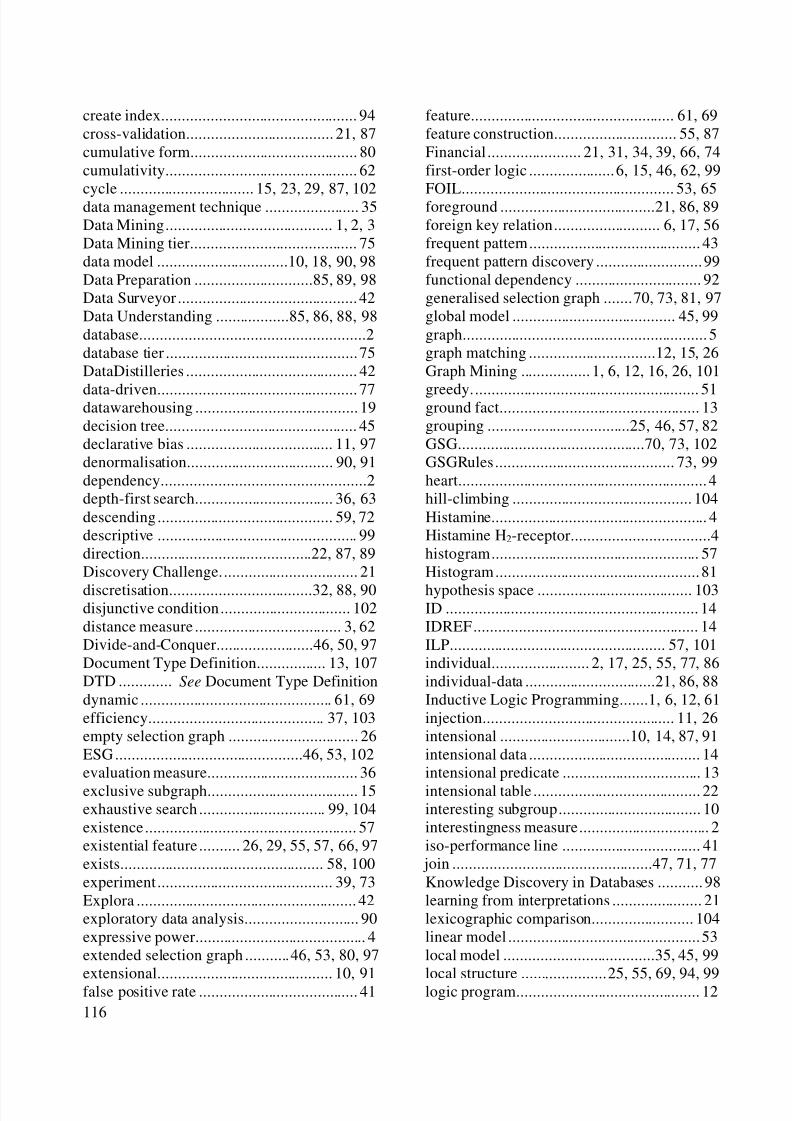
8/8/2019 Knobbe a.J. Multi-Relational Data Mining
http://slidepdf.com/reader/full/knobbe-aj-multi-relational-data-mining 127/129
116
create index................................................ 94cross-validation.................................... 21, 87cumulative form......................................... 80cumulativity............................................... 62
cycle ................................. 15, 23, 29, 87, 102data management technique ....................... 35Data Mining......................................... 1, 2, 3Data Mining tier......................................... 75data model ................................10, 18, 90, 98Data Preparation .............................85, 89, 98Data Surveyor............................................ 42Data Understanding ..................85, 86, 88, 98database.......................................................2database tier ............................................... 75DataDistilleries .......................................... 42
data-driven................................................. 77datawarehousing ........................................ 19decision tree............................................... 45declarative bias .................................... 11, 97denormalisation.................................... 90, 91dependency..................................................2depth-first search.................................. 36, 63descending........................................... 59, 72descriptive ................................................. 99direction..........................................22, 87, 89Discovery Challenge.................................. 21
discretisation...................................32, 88, 90disjunctive condition................................ 102distance measure .................................... 3, 62Divide-and-Conquer........................46, 50, 97Document Type Definition................. 13, 107DTD ............. See Document Type Definitiondynamic ............................................... 61, 69efficiency........................................... 37, 103empty selection graph ................................ 26ESG ..............................................46, 53, 102evaluation measure..................................... 36
exclusive subgraph..................................... 15exhaustive search............................... 99, 104existence.................................................... 57existential feature.......... 26, 29, 55, 57, 66, 97exists.................................................. 58, 100experiment........................................... 39, 73Explora ...................................................... 42exploratory data analysis............................ 90expressive power.......................................... 4extended selection graph ...........46, 53, 80, 97extensional........................................... 10, 91false positive rate ....................................... 41
feature.................................................. 61, 69feature construction.............................. 55, 87Financial....................... 21, 31, 34, 39, 66, 74first-order logic .....................6, 15, 46, 62, 99
FOIL.................................................... 53, 65foreground ......................................21, 86, 89foreign key relation.......................... 6, 17, 56frequent pattern.......................................... 43frequent pattern discovery .......................... 99functional dependency ............................... 92generalised selection graph .......70, 73, 81, 97global model ........................................ 45, 99graph............................................................ 5graph matching ...............................12, 15, 26Graph Mining ................. 1, 6, 12, 16, 26, 101
greedy........................................................ 51ground fact................................................. 13grouping ...................................25, 46, 57, 82GSG..............................................70, 73, 102GSGRules............................................ 73, 99heart............................................................. 4hill-climbing ............................................ 104Histamine..................................................... 4Histamine H2-receptor..................................4histogram................................................... 57Histogram.................................................. 81
hypothesis space ...................................... 103ID .............................................................. 14IDREF ....................................................... 14ILP..................................................... 57, 101individual........................ 2, 17, 25, 55, 77, 86individual-data ................................21, 86, 88Inductive Logic Programming.......1, 6, 12, 61injection............................................... 11, 26intensional ................................10, 14, 87, 91intensional data .......................................... 14intensional predicate .................................. 13
intensional table ......................................... 22interesting subgroup................................... 10interestingness measure................................ 2iso-performance line .................................. 41 join .................................................47, 71, 77Knowledge Discovery in Databases ........... 98learning from interpretations ...................... 21lexicographic comparison......................... 104linear model ............................................... 53local model .....................................35, 45, 99local structure .....................25, 55, 69, 94, 99logic program............................................. 12
8/8/2019 Knobbe a.J. Multi-Relational Data Mining
http://slidepdf.com/reader/full/knobbe-aj-multi-relational-data-mining 128/129
117
look-ahead ....................................51, 80, 104look-ahead association refinement........ 52, 81look-ahead condition refinement .......... 51, 80look-up ...................................................... 56
look-up table .............................................. 88many-to-many............................................ 21many-to-one............................................... 91max...................................................... 57, 59maximum........................................31, 57, 79meta-data ..................................................... 4MIDOS...................................................... 42MIDOS.................................................... 104min ...................................................... 57, 59minimum ........................................31, 57, 79mining structured data................................ 16
mode declaration........................................ 13model...........................................................2molecule .....................................5, 10, 15, 47Monet .................................................. 37, 76monotonic.......................................... 72, 104monotonicity............................................ 104MRDM ..... See Multi-Relational Data MiningMRDM pre-processing consultant........ 90, 98MRDM project..................................... 85, 98MRDTL............................................... 52, 99
107, See Multi-Relational
Modelling LanguageMr-SMOTI ................................................ 53multiple-instance........................................ 64multiplicity .....................................18, 56, 94Multi-Relational Data Mining .......1, 6, 16, 97
50, 77, 98multi-relational decision tree................ 45, 50Multi-Relational Modelling Language.. 19, 97Musk.......................................................... 64Mutagenesis ..............................52, 58, 65, 73
mutually exclusive subgroup................ 30, 45MySQL...................................................... 39nested aggregate function......................... 103nominal attribute .................................. 30, 59NominalCrossTable ........................37, 78, 81non-determinacy .................................. 69, 99non-monotonic refinement ....................... 102non-monotonic refinement operator ......... 104non-monotonic search.............................. 102normalisation ............................................. 92novelty......................................36, 38, 40, 73numeric...................................................... 14
numeric attribute.................................. 39, 79numeric data ...................................30, 31, 88numeric value ............................................ 62NumericCrossTable ............................. 79, 83
OLAP ........................................................ 19one-to-many..............................21, 25, 64, 94open..................................................... 46, 70optimal refinement operator ..................... 103OptimalRefinement.................................... 50optimistic estimate ............................. 42, 104order .......................................................... 14outer join.................................................... 56parallelisation............................................. 99part .............................................................. 9pattern........................................................ 10
pattern language......................10, 69, 97, 101playing card ............................................... 31Poker ......................................................... 15Polka...............................................62, 64, 99predicate .................................................... 12predictive ...................................................99predictive model .................................... 2, 45pre-processing...................................... 58, 99present ................................................. 46, 49presentation tier ......................................... 75primary key................................................ 93
priority queue............................................. 36Progol .................................................. 53, 65project blueprint......................................... 85Prolog ........................................................ 13propagated key........................................... 67propositional ................................................ 3Propositional Data Mining ...........................3propositionalisation.............59, 61, 67, 90, 99ProSafarii............................................. 90, 98
See Relational DatabaseManagement Systems
Receiver Operating Characteristics............. 41recursion.........................................15, 87, 89redundancy .............................................. 103redundant association................................. 23refinement.................................................. 12refinement depth ...................................... 104refinement operator........... 12, 27, 69, 71, 102refinement-depth......... 29, 39, 57, 66, 92, 100regression............................................. 52, 62regression tree............................................ 53RELAGGS........................................... 65, 67Relational Data Mining .............................. 16
multi-relational data mining primitive........ 37,
MRML...............90,
RDBMS...............76,
8/8/2019 Knobbe a.J. Multi-Relational Data Mining
http://slidepdf.com/reader/full/knobbe-aj-multi-relational-data-mining 129/129
relational database................................ 15, 25relational database management system ....... 6relational database theory............................. 1Relational Learning.................................... 16
relational model ...........................................6relational probability tree ........................... 69representation....................................... 14, 46retail database ............................................ 93reverse pivot .............................................. 93ROC analysis ............................................. 41RollUp............................................63, 65, 99rule ...................................................... 40, 73Rule Discovery .............................35, 69, 103Safarii.................................37, 39, 75, 90, 98sampling .................................................... 21
scalability................................................... 75schema.........................................................9score function ........................................ 2, 11search process .................................22, 37, 77search space ........................................... 5, 61search strategy ........................................... 35select attribute............................................ 94select table ................................................. 94selection edge ............................................ 27selection graph................................26, 77, 97selection node ............................................ 26
semi-automated.......................................... 90Semi-Structured Data Mining........... 6, 13, 16semi-structured text.................................... 13sensitivity............................................. 36, 40SG ................................................70, 73, 101SGRules..........................................37, 73, 99SMOTI ...................................................... 53
Structured Query Language..........................6structured term........................................... 14subgraph .................................................... 11subgroup.....................................2, 11, 32, 77
sum............................................................ 59support................................................. 36, 40tag.............................................................. 13target attribute............................................ 38target concept....................................... 86, 88target table ......................................17, 20, 61Tertius ............................................... 42, 104test set........................................................ 87threshold.................................................... 31Tilde .........................................19, 52, 53, 65Tilde-RT.................................................... 53
top-down algorithm............................ 69, 102top-down induction.................................... 4628, 49,
71,72top-down search................................. 12, 104training ...................................................... 87transaction ........................................... 39, 66transformation............................................ 90transformation rule..................................... 91TranslateExtendedSelectionGraph.............. 47TranslateSelectionGraph ............................ 27
TranslateSubgraph ............................... 47, 80true positive rate......................................... 41tuple............................................................. 9UML........... See Unified Modeling Languageunfold recursion......................................... 87Unified Modeling Language................. 19, 97universal quantification............................ 102
top-down refinement operator.........12,