KeystoneML: Optimizing Pipelines for Large-ScaleAdvanced Analytics

Evan R. Sparks, Shivaram Venkataraman, Tomer Kaftan, Michael Franklin, Benjamin RechtAMPLab, University of California, Berkeley,

{sparks,shivaram,tomerk11,franklin,brecht}@cs.berkeley.edu

AbstractModern advanced analytics applications make use ofmachine learning techniques and contain multiple stepsof domain-specific and general-purpose processing withhigh resource requirements. We present KeystoneML, asystem that captures and optimizes the end-to-end large-scale machine learning applications for high-throughputtraining in a distributed environment with a high-levelAPI. This approach offers increased ease of use andhigher performance over existing systems for large scalelearning. We demonstrate the effectiveness of Key-stoneML in achieving high quality statistical accuracyand scalable training using real world datasets in sev-eral domains. By optimizing execution KeystoneMLachieves up to 15× training throughput over unoptimizedexecution on a real image classification application.

1 IntroductionToday’s advanced analytics applications increasingly usemachine learning (ML) as a core technique in areasranging from business intelligence to recommendationto natural language processing [39] and speech recog-nition [29]. Practitioners build complex, multi-stagepipelines involving feature extraction, dimensionality re-duction, data transformations, and training supervisedlearning models to achieve high accuracy [52]. However,current systems provide little support for automating theconstruction and optimization of these pipelines.

To assemble such pipelines, developers typically piecetogether domain specific libraries1 for feature extrac-tion and general purpose numerical optimization pack-ages [34, 44] for supervised learning. This is often acumbersome and error-prone process [53]. Further, thesepipelines need to be completely re-engineered when thetraining data or features grow by an order of magnitude–often the difference between an application that providesgood statistical accuracy and one that does not [23]. As

1e.g. OpenCV for Images (http://opencv.org/), Kaldi for Speech(http://kaldi-asr.org/)

1. Pipeline Specification 2. Logical Operator DAG

3. Optimized Physical DAG 4. Distributed Training

val pipe = Preprocess andThen Featurize andThen (Est, data, labels)

Figure 1: KeystoneML takes a high-level ML applica-tion specification, optimizes and trains it in a distributedenvironment. The trained pipeline is used to make pre-dictions on new data.

no broader system has purview of the end-to-end appli-cation, only narrow optimizations can be applied.

These challenges motivate the need for a system that

• Allows users to specify end-to-end ML applicationsin a single system using high level logical operators.

• Scales out dynamically as data volumes and prob-lem complexity change.

• Automatically optimizes these applications given alibrary of ML operators and the user’s compute re-sources.

While existing efforts in the data management com-munity [27, 21, 44] and in the broader machine learningsystems community [34, 45, 3] have built systems to ad-dress some of these problems, each of them misses themark on at least one of the points above.

We present KeystoneML, a framework for MLpipelines designed to satisfy the above requirements.Fundamental to the design of KeystoneML is the obser-vation that model training is only one component of anML application. While a significant body of recent workhas focused on high performance algorithms [61, 50],

1

arX

iv:1

610.

0945

1v1

[cs

.LG

] 2

9 O

ct 2

016

and scalable implementations [17, 44] for model train-ing, they do not capture the featurization process or thelogical intent of the workflow. KeystoneML provides ahigh-level, type-safe API built around logical operatorsto capture end-to-end applications.

To optimize ML pipelines, database query optimiza-tion provides a natural motivation for the core designof such a system [32]. However, compared to relationaldatabase query optimization, ML applications present anadditional set of concerns. First, ML operators are of-ten iterative and may require multiple passes over theirinputs, presenting opportunities for data reuse. Second,many ML operators provide only approximate answers totheir inputs [50]. Third, numerical data properties suchas sparsity and dimensionality are a necessary source ofinformation when selecting optimal execution plans andconventional optimizers do not consider such measures.Finally, the system should be aware of the computation-vs-communication tradeoffs inherent in distributed pro-cessing of ML workloads [21, 34] and choose appropri-ate execution strategies in this regime.

To address these challenges we develop techniquesto do both per-operator optimization and end-to-endpipeline optimization for ML pipelines. We use a cost-based optimizer that accounts for both computation andcommunication costs and our cost model can easily ac-commodate new operators and hardware configurations.To determine which intermediate states are materializedin memory during iterative execution, we formulate anoptimization problem and present a greedy algorithmthat works efficiently and accurately in practice.

We measure the importance of cost-based optimiza-tion and its associated overheads using real-world work-loads from computer vision, speech and natural languageprocessing. We find that end-to-end optimization canimprove performance by 7× and that physical operatoroptimizations combined with end-to-end optimizationscan improve performance by up to 15× versus unopti-mized execution. We show that in our experiments, poorphysical operator selection can result in up to a 260×slowdown. Using an image classification pipeline onover 1M images [52], we show that KeystoneML pro-vides linear performance scalability across various clus-ter sizes, and statistical performance comparable to re-cent results [11, 52]. Additionally, KeystoneML canmatch the performance of a specialized phoneme classifi-cation system on a BlueGene supercomputer while using8× fewer resources. In summary, we make the followingcontributions:

• We present KeystoneML, a system for describingML applications using high level logical opera-tors. KeystoneML enables end-to-end optimizationof ML applications at both the operator and pipelinelevel.

val textClassifier = Trim andThenLowerCase andThenTokenizer andThenNGramsFeaturizer(1 to 2) andThenTermFrequency(x => 1) andThen(CommonSparseFeatures(1e5), data) andThen(LinearSolver(), data, labels)

val predictions = textClassifier(testData)

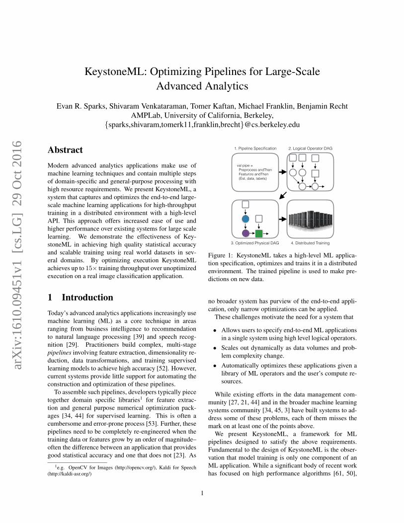
Figure 2: A text classification pipeline is specified usinga small set of logical operators.

• We demonstrate the importance of physical opera-tor selection in the context of input characteristicsof three commonly used logical ML operators, andpropose a cost model for making this selection.

• We present and evaluate an initial set of whole-pipeline optimizations, including a novel algorithmthat automatically identifies a subset of intermediatedata to materialize to speed up pipeline execution.

• We evaluate these optimizations in the context ofreal-world pipelines in a diverse set of domains:phoneme classification, image classification, andtextual sentiment analysis, and demonstrate near-linear scalability over 100s of machines with strongstatistical performance.

• We compare KeystoneML with several recent sys-tems for large-scale learning and demonstrate supe-rior runtime from our optimization techniques andscale-out strategy.

KeystoneML is open source software2 and is beingused in scientific applications in solar physics [30] andgenomics [2]

2 Pipeline Construction and CoreAPIs

In this section we introduce the KeystoneML API thatcan be used to express end-to-end ML pipelines. Eachpipeline is composed a number of operators that arechained together. For example, Figure 2 shows the Key-stoneML source code for a complete text classificationpipeline. We next describe the building blocks of ourAPI.

2.1 Logical ML OperatorsConventional analytics queries are typically composedusing a small number of well studied relational databaseoperators. This well-defined environment enables im-portant optimizations. However, ML applications lacksuch an abstraction and practitioners typically piece to-gether imperative libraries. Recent efforts have proposed

2http://www.keystone-ml.org/

2

trait Transformer[A, B] extends Pipeline[A, B] {def apply(in: Dataset[A]): Dataset[B] =in.map(apply)

def apply(in: A): B}

trait Estimator[A, B] {def fit(data: Dataset[A]): Transformer[A, B]

}

trait Optimizable[T, A, B] {val options: List[(CostModel, T[A,B])]def optimize(sample: Dataset[A], d: ResourceDesc):

T[A,B]}

class CostProfile(flops: Long, bytes: Long, network: Long)

trait CostModel {def cost(sample: Dataset[A], workers: Int):

CostProfile}

trait Iterative {def weight: Int

}

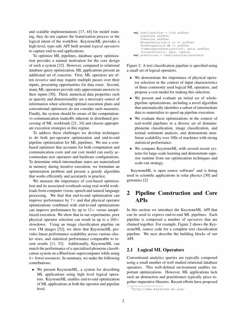
Figure 3: The KeystoneML API consists of two extend-able operator types and interfaces for optimization.

using linear algebra operators such as matrix multipli-cation [21], convex optimization routines [20] or multi-dimensional arrays as logical building blocks [57].

In contrast, with KeystoneML we propose a de-sign where high-level ML operations (such as PCA,LinearSolver) are used as building blocks. Our ap-proach has two major benefits: First, it simplifies build-ing applications. Even complex pipelines can be built us-ing just a handful of operators. Second, this higher levelabstraction allows us to perform a wider range of opti-mizations. Our key insight here is that there are usuallymultiple well studied algorithms for a given ML opera-tor, but that their performance and statistical characteris-tics vary based on the inputs and system configuration.We next describe the API for operators in KeystoneML.

Pipelines are composed of operators. Transformersand Estimators are two abstract types of operators inKeystoneML. An operator is a function which operateson zero or more inputs to produce some output. A logicaloperator satisfies some logical contract. For example, ittakes an image and converts it to grayscale. Every logicaloperator must have at least one physical operator asso-ciated with it which implements its logic. Logical oper-ators with multiple physical implementations are candi-dates for optimization. They are marked Optimizableand have a set of CostModels associated with them.Operators that are iterative with respect to their inputsare marked Iterative.

A Transformer is an operator that can be applied toindividual data items (or to a collection of items) andproduces a new data item (or a collection of data items)–it is a deterministic unary function without side-effects.

trait Pipeline[A,B] {def andThen[C](

next: Pipeline[B, C]): Pipeline[A, C]def andThen[C](

est: Estimator[B, C],data: Dataset[A]): Pipeline[A, C]

// Combine the outputs of branches// into a sequencedef gather[A, B](branches: Seq[Pipeline[A, B]]):

Pipeline[A, Seq[B]]}

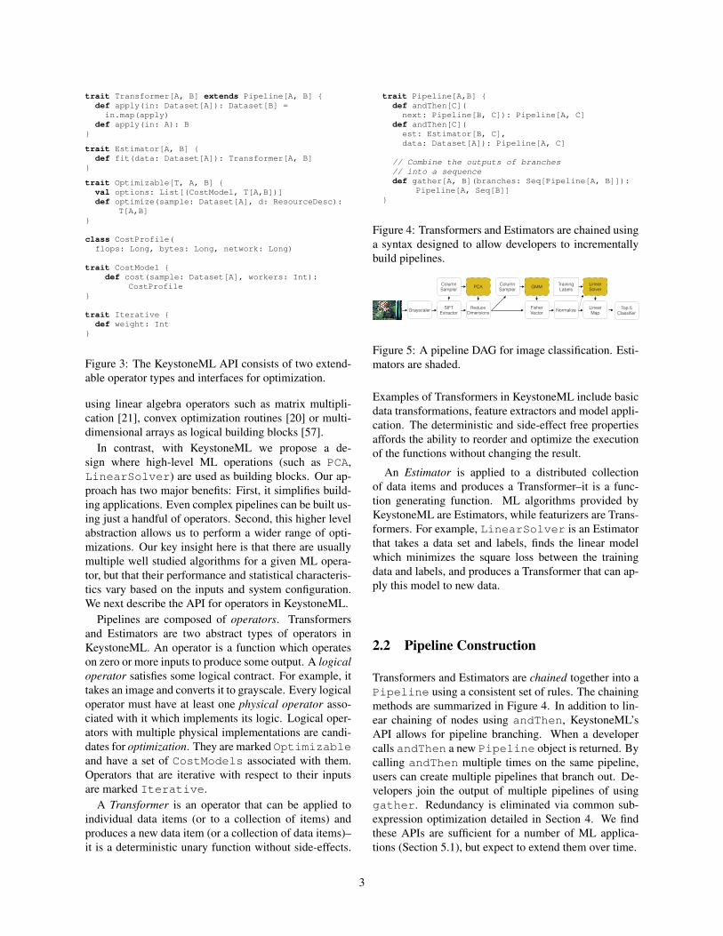
Figure 4: Transformers and Estimators are chained usinga syntax designed to allow developers to incrementallybuild pipelines.

Grayscaler SIFT Extractor

Reduce Dimensions

Fisher Vector Normalize

Column Sampler

Linear Map

PCA Column Sampler GMM Linear

Solver

Grayscale

PCA GMM

SIFTWeighted

Linear Solver

Top 5 Classifier

Fisher Vector Normalize Top 5 Classifier

Training Labels

Figure 5: A pipeline DAG for image classification. Esti-mators are shaded.

Examples of Transformers in KeystoneML include basicdata transformations, feature extractors and model appli-cation. The deterministic and side-effect free propertiesaffords the ability to reorder and optimize the executionof the functions without changing the result.

An Estimator is applied to a distributed collectionof data items and produces a Transformer–it is a func-tion generating function. ML algorithms provided byKeystoneML are Estimators, while featurizers are Trans-formers. For example, LinearSolver is an Estimatorthat takes a data set and labels, finds the linear modelwhich minimizes the square loss between the trainingdata and labels, and produces a Transformer that can ap-ply this model to new data.

2.2 Pipeline Construction

Transformers and Estimators are chained together into aPipeline using a consistent set of rules. The chainingmethods are summarized in Figure 4. In addition to lin-ear chaining of nodes using andThen, KeystoneML’sAPI allows for pipeline branching. When a developercalls andThen a new Pipeline object is returned. Bycalling andThen multiple times on the same pipeline,users can create multiple pipelines that branch out. De-velopers join the output of multiple pipelines of usinggather. Redundancy is eliminated via common sub-expression optimization detailed in Section 4. We findthese APIs are sufficient for a number of ML applica-tions (Section 5.1), but expect to extend them over time.

3

2.3 Pipeline Execution

KeystoneML is designed to run with large, distributeddatasets on commodity clusters. Our high level APIand optimizers can be executed using any distributeddata-flow engine. The execution flow of KeystoneMLis shown in Figure 1. First, developers specify pipelinesusing the KeystoneML APIs described above. As calls tothese APIs are made, KeystoneML incrementally buildsan operator DAG for the pipeline. An example operatorDAG for image classification is shown in Figure 5. Oncea pipeline is applied to some data, this DAG is then op-timized using a set of optimizations described below–wecall this stage optimization time. Once the applicationhas been optimized, the DAG is traversed depth-first andoperators are executed one at a time, with nodes up untilpipeline breakers (i.e. Estimators) packed into the samejob–this stage is runtime. This lazy optimization proce-dure gives the optimizer full information about the appli-cation in question. We now consider the optimizationsmade by KeystoneML.

3 Operator-Level Optimization

In this section we describe the operator-level optimiza-tion procedure used in KeystoneML. Similar to databasequery optimizers, the goal of the operator-level optimizeris to choose the best physical implementation for everymachine learning operator in the pipeline. This is chal-lenging to do because operators in KeystoneML are dis-tributed i.e. they involve computation and communica-tion across the cluster. Operator performance may alsodepend on statistical properties like sparsity of input dataand level of accuracy desired. Finally, as discussed inSection 2, KeystoneML consists of a set of high-leveloperators. The advantage of having high-level operatorsis that we can perform more wide-ranging optimizations.But this makes designing an optimizer more challengingbecause unlike relational operators or linear algebra [21],the set of operators in KeystoneML is not closed. Wenext discuss how we address these challenges.Approach: The approach we take in KeystoneML is todevelop a cost-based optimizer that splits the cost modelinto two parts: an operator-specific part and a cluster-specific part. The operator-specific part models the com-putation and communication time given statistics of theinput data and number of workers and the cluster specificpart is used to weigh their relative importance. More for-mally, the cost estimate for each physical operator, f canbe expressed as:

c(f,As, R) = Rexeccexec(f,As, Rw)+ (1)Rcoordccoord(f,As, Rw) (2)

Algorithm Compute Network Memory

Local QR O(nd(d+ k)) O(n(d+ k)) O(d(n+ k))

Dist. QR O(nd(d+k)

w) O(d(d+ k)) O(nd

w+ d2)

L-BFGS O( inskw

) O(idk) O(nsw

+ dk)

Block Solve O(ind(b+k)

w) O(id(b+ k)) O(nb

w+ dk)

Table 1: Resource requirements for linear solvers. w isthe number of workers in the cluster, i the number ofpasses over the dataset. For the sparse solvers s is thethe average number of non-zero features per example,and b is the block size for the block solver. Computeand Memory requirements are per-node, while networkrequirements are in terms of the data sent over the mostloaded link.

Where f is the operator in question,As contains statis-tics of a dataset to be used as its input, and R, the clus-ter resource descriptor represents the cluster computing,memory, and networking resources available. The clus-ter resource descriptor is collected via configuration dataand microbenchmarks. Statistics captured include per-node CPU throughput (in GFLOP/s), disk and memorybandwidth (GB/s), and network speed (GB/s), as wellas information about the number of nodes available. Asis determined through a process we will discuss in Sec-tion 4. Rw is the number of cluster nodes available.

The functions, cexec, and ccoord are developer-definedoperator-specific functions (defined as part of the oper-ator CostModel) that describe execution and coordi-nation costs in terms of the longest critical path in theexecution graph of the individual operators [59], e.g.the most FLOPS used by a node in the cluster or theamount of data transferred over the most loaded link.Such functions are also used in the analysis of parallelalgorithms [6] and are well known for common linear al-gebra based operators. Rexec and Rcoord are determinedby the optimizer from the cluster resource descriptor (R)and capture the relative speed of local and network re-sources on the cluster.

Splitting the cost model in this fashion allows the theoptimizer to easily adapt to new hardware (e.g., GPUsor Infiniband networks) and also for it to work with bothexisting and future operators. Operator developers onlyneed to implement a CostModel and the system ac-counts for hardware properties. Finally we note that thecost model we use here is approximate and that the costc need not be equal to the actual running time of the op-erator. Rather, as in conventional query optimizers, thegoal of the cost model is to avoid bad decisions, which aroughly accurate model will do. At the boundary of twonearly equivalent operators, either should be acceptablein terms of runtime. We next illustrate the cost functionsfor three central operators in KeystoneML and the perfor-mance trade-offs that arise from varying input properties.

4

Linear Solvers are supervised Estimators that learn alinear map X between an input dataset A in Rn×d to alabels dataset B in Rn×k by finding the X which mini-mizes the value ||AX−B||F . In a multi-class classifica-tion setting, n is the number of examples or data points,d the number of features and k the number of classes. Inthe KeystoneML Standard Library we have several im-plementations of linear solvers, distributed and local, in-cluding

• Exact solvers [18] that compute closed form solu-tions to the least squares loss and return an X toextremely high precision.

• Block solvers that partition the features into a setof blocks and use second-order Jacobi or Gauss-Seidel [9] updates to converge to the right solution.

• Gradient based methods like SGD [50] or L-BFGS [14] which perform iterative updates usingthe gradient and converge to a globally optimal so-lution.

Table 1 summarizes the cost model for each method.Constants are omitted for readability but are necessaryin practice.

To illustrate these cost tradeoffs empirically, we varythe number of features generated by the featurizationstage of two different pipelines and measure the train-ing time and the training loss. We compare the methodson a 16 node cluster.

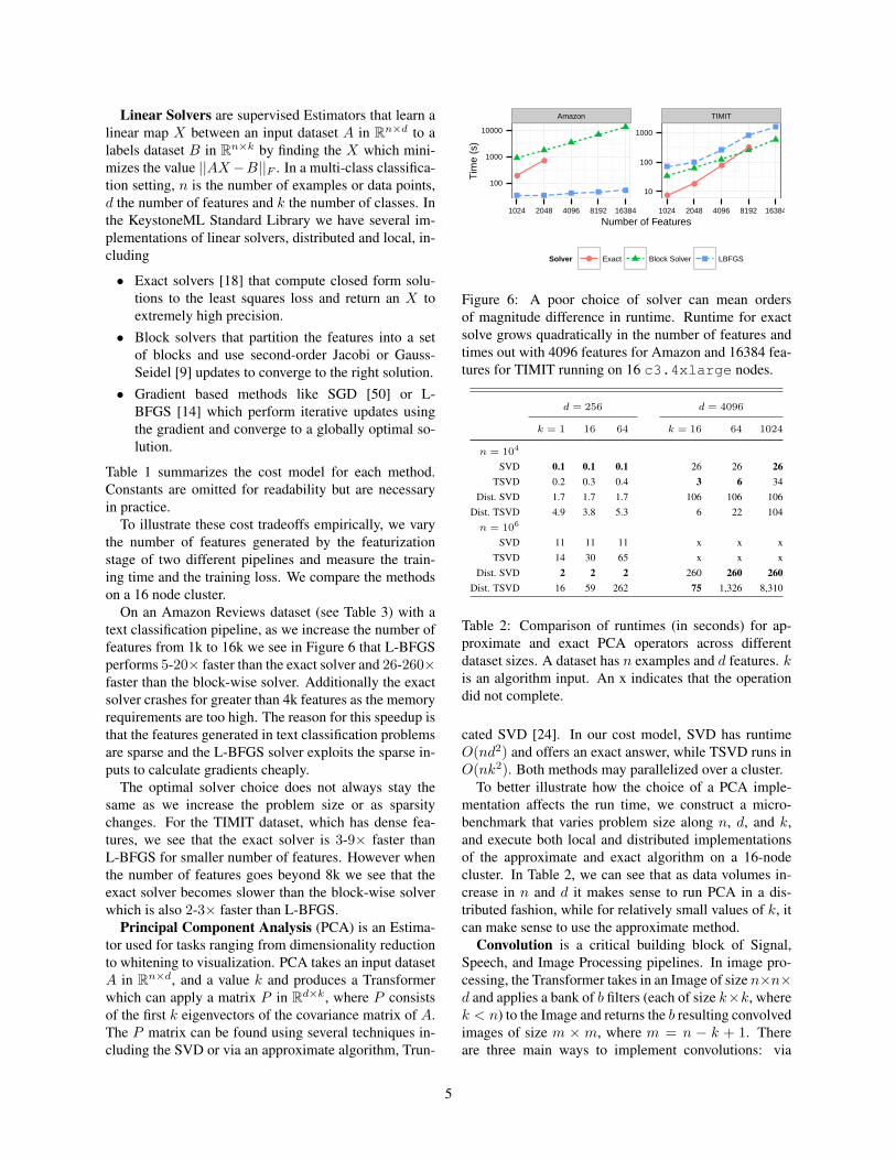
On an Amazon Reviews dataset (see Table 3) with atext classification pipeline, as we increase the number offeatures from 1k to 16k we see in Figure 6 that L-BFGSperforms 5-20× faster than the exact solver and 26-260×faster than the block-wise solver. Additionally the exactsolver crashes for greater than 4k features as the memoryrequirements are too high. The reason for this speedup isthat the features generated in text classification problemsare sparse and the L-BFGS solver exploits the sparse in-puts to calculate gradients cheaply.

The optimal solver choice does not always stay thesame as we increase the problem size or as sparsitychanges. For the TIMIT dataset, which has dense fea-tures, we see that the exact solver is 3-9× faster thanL-BFGS for smaller number of features. However whenthe number of features goes beyond 8k we see that theexact solver becomes slower than the block-wise solverwhich is also 2-3× faster than L-BFGS.

Principal Component Analysis (PCA) is an Estima-tor used for tasks ranging from dimensionality reductionto whitening to visualization. PCA takes an input datasetA in Rn×d, and a value k and produces a Transformerwhich can apply a matrix P in Rd×k, where P consistsof the first k eigenvectors of the covariance matrix of A.The P matrix can be found using several techniques in-cluding the SVD or via an approximate algorithm, Trun-

●

●

●

●

●

●

Amazon TIMIT

100

1000

10000

10

100

1000

1024 2048 4096 8192 16384 1024 2048 4096 8192 16384

Number of Features

Tim

e (s

)

Solver ● Exact Block Solver LBFGS

Figure 6: A poor choice of solver can mean ordersof magnitude difference in runtime. Runtime for exactsolve grows quadratically in the number of features andtimes out with 4096 features for Amazon and 16384 fea-tures for TIMIT running on 16 c3.4xlarge nodes.

d = 256 d = 4096

k = 1 16 64 k = 16 64 1024

n = 104

SVD 0.1 0.1 0.1 26 26 26TSVD 0.2 0.3 0.4 3 6 34

Dist. SVD 1.7 1.7 1.7 106 106 106Dist. TSVD 4.9 3.8 5.3 6 22 104n = 106

SVD 11 11 11 x x xTSVD 14 30 65 x x x

Dist. SVD 2 2 2 260 260 260Dist. TSVD 16 59 262 75 1,326 8,310

Table 2: Comparison of runtimes (in seconds) for ap-proximate and exact PCA operators across differentdataset sizes. A dataset has n examples and d features. kis an algorithm input. An x indicates that the operationdid not complete.

cated SVD [24]. In our cost model, SVD has runtimeO(nd2) and offers an exact answer, while TSVD runs inO(nk2). Both methods may parallelized over a cluster.

To better illustrate how the choice of a PCA imple-mentation affects the run time, we construct a micro-benchmark that varies problem size along n, d, and k,and execute both local and distributed implementationsof the approximate and exact algorithm on a 16-nodecluster. In Table 2, we can see that as data volumes in-crease in n and d it makes sense to run PCA in a dis-tributed fashion, while for relatively small values of k, itcan make sense to use the approximate method.

Convolution is a critical building block of Signal,Speech, and Image Processing pipelines. In image pro-cessing, the Transformer takes in an Image of size n×n×d and applies a bank of b filters (each of size k×k, wherek < n) to the Image and returns the b resulting convolvedimages of size m × m, where m = n − k + 1. Thereare three main ways to implement convolutions: via

5

●●

●●

● ● ● ● ● ● ● ●●●●

100

1000

10000

2 4 6 10 20 30

Convolution Size (k)

Tim

e (m

s)

Strategy ● Separable BLAS FFT

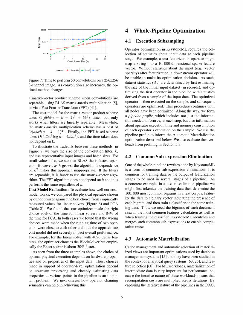
Figure 7: Time to perform 50 convolutions on a 256x2563-channel image. As convolution size increases, the op-timal method changes.

a matrix-vector product scheme when convolutions areseparable, using BLAS matrix-matrix multiplication [5],or via a Fast Fourier Transform (FFT) [41].

The cost model for the matrix-vector product schemetakes O(dbk(n − k + 1)2 + bk3) time, but onlyworks when filters are linearly separable. Meanwhile,the matrix-matrix multiplication scheme has a cost ofO(dbk2(n − k + 1)2). Finally, the FFT based schemetakes O(6dbn2 log n + 4dbn2), and the time taken doesnot depend on k.

To illustrate the tradeoffs between these methods, inFigure 7, we vary the size of the convolution filter, k,and use representative input images and batch sizes. Forsmall values of k, we see that BLAS the is fastest oper-ator. However, as k grows, the algorithm’s dependenceon k2 makes this approach inappropriate. If the filtersare separable, it is faster to use the matrix-vector algo-rithm. The FFT algorithm does not depend on k and thusperforms the same regardless of k.Cost Model Evaluation: To evaluate how well our cost-model works, we compared the physical operator chosenby our optimizer against the best choice from empiricallymeasured values for linear solvers (Figure 6) and PCA(Table 2). We found that our optimizer made the rightchoice 90% of the time for linear solvers and 84% ofthe time for PCA. In both cases we found that the wrongchoices were made when the running time of two oper-ators were close to each other and thus the approximatecost model did not severely impact overall performance.For example, for the linear solver with 4096 dense fea-tures, the optimizer chooses the BlockSolver but empiri-cally the Exact solver is about 30% faster.

As seen from the three examples above, the choice ofoptimal physical execution depends on hardware proper-ties and on properties of the input data. Thus, choicesmade in support of operator-level optimization dependon upstream processing and cheaply estimating dataproperties at various points in the pipeline is an impor-tant problem. We next discuss how operator chainingsemantics can help in achieving this.

4 Whole-Pipeline Optimization

4.1 Execution Subsampling

Operator optimization in KeystoneML requires the col-lection of statistics about input data at each pipelinestage. For example, a text featurization operator mightmap a string into a 10, 000-dimensional sparse featurevector. Without statistics about the input (e.g. vectorsparsity) after featurization, a downstream operator willbe unable to make its optimization decision. As such,dataset statistics (As) are determined by first estimatingthe size of the initial input dataset (in records), and op-timizing the first operator in the pipeline with statisticsderived from a sample of the input data. The optimizedoperator is then executed on the sample, and subsequentoperators are optimized. This procedure continues untilall nodes have been optimized. Along the way, we forma pipeline profile, which includes not just the informa-tion needed to form As at each step, but also informationabout operator execution time and memory consumptionof each operator’s execution on the sample. We use thepipeline profile to inform the Automatic Materializationoptimization described below. We also evaluate the over-heads from profiling in Section 5.3.

4.2 Common Sub-expression Elimination

One of the whole-pipeline rewrites done by KeystoneMLis a form of common sub-expression elimination. It iscommon for training data or the output of featurizationstages to be used in several stages of a pipeline. Asa concrete example, in a text classification pipeline wemight first tokenize the training data then determine the100, 000 most common bigrams in a text corpus, featur-ize the data to a binary vector indicating the presence ofeach bigram, and then train a classifier on the same train-ing data. Thus, we need the bigrams of each documentboth in the most common features calculation as well aswhen training the classifier. KeystoneML identifies andmerges such common sub-expressions to enable compu-tation reuse.

4.3 Automatic Materialization

Cache management and automatic selection of material-ized views are important optimizations used by databasemanagement systems [15] and they have been studied inthe context of analytical query systems [63, 25], and fea-ture selection [60]. For ML workloads, materialization ofintermediate data is very important for performance be-cause the iterative nature of these workloads means thatrecomputation costs are multiplied across iterations. Bycapturing the iterative nature of the pipelines in the DAG,

6

our optimizer is capable of identifying opportunities forreuse, eliminating redundant computation. We next de-scribe a formulation for the materialization problem initerative pipelines and propose an algorithm to automati-cally select a good set of intermediate objects to materi-alize in order to speed up ML pipeline execution.

Given the depth-first execution model and the deter-ministic and side-effect free nature of KeystoneML op-erators, a natural strategy is materialization of operatoroutputs that are visited multiple times during the exe-cution. This optimization works well in the absence ofmemory constraints.

However, in many applications we have built withKeystoneML, intermediate output can grow to multipleterabytes in size, even for modestly sized inputs. Oncurrent hardware, this output is too big to fit in mem-ory, even with hundreds of GB of memory per machine.Commonly used caching policies such as LRU can resultin suboptimal run times because the decision to cachea large object (e.g. intermediate features) may evict asmaller object that is needed later in the pipeline and maybe expensive to recompute (e.g. image features).

We propose an algorithm to automatically select theitems to cache in the presence of memory constraints,given that we know how often the objects will be ac-cessed, that we can estimate their size, and that we canestimate the runtime associated with materializing them.

We formulate the problem as follows: Given a mem-ory budget, we want to find the set of nodes to include inthe cache set that minimizes total execution time.

Let v be our node of interest in a pipeline G, t(v) isthe time taken to do the computation that is local to nodev per iteration, C(v) is the number of times a node willby called by its direct successors during execution, andwv is the number of times a node iterates over its inputs.T (n), the total execution time of the pipeline up to andincluding node v is:

T (v) =

wv(t(v) +∑

c∈χ(v)T (c))

C(v)κv

where κv ∈ {0, 1} is a binary indicator variable signify-ing whether a node is cached or not, and χ(v) representsthe direct predecessors of v in the DAG.

Where C(v) is defined as follows:

C(v) =

∑

p∈π(v)wpC(p)

κp , |π(v)| > 0

1, otherwise

where π(v) represents the direct successors of v in theDAG. Because of the DAG structure of the pipelinegraph, we are guaranteed to not have any cycles in thisgraph, thus both T (v) and C(v) are well-defined.

1 Algorithm GreedyOptimizer:input : G, t, size, memSizeoutput: cache

2 cache← ∅;3 memLeft← memSize;4 next← pickNext (G, cache, size, memLeft, t);5 while nextNode 6= ∅ do6 cache← cache ∪ next;7 memLeft← memLeft - size(next);8 next← pickNext (G, cache, size, memLeft, t);9 end

10 return cache;11 end

1 Procedure pickNext:input : G, cache, size, memLeft, toutput: next

2 minTime←∞;3 next← ∅;4 for v ∈ nodes(G) do5 runtime← estRuntime (G, cache ∪ v, t);6 if runtime < minTime & size(v) < memLeft then7 next← v;8 minTime← runtime;9 end

10 end11 return next;12 end

Algorithm 1: The caching algorithm in KeystoneMLbuilds a cache set by finding the node that willmaximize time saved subject to memory constraints.estRuntime is a procedure that computes T (v) fora given DAG, cache set, and node.

We can state the problem of minimizing pipeline ex-ecution time formally as an optimization problem withlinear constraints as follows:

minκT (sink(G))

s.t.∑v∈V

size(v)κv ≤ memSize

Where sink(G) is the pipeline terminus, size(v) thesize of v’s output, andmemSize the memory constraint.

This problem can also be thought of as problem offinding an optimal cache schedule. It is tempting to reachfor classical results [7, 48] in the optimal paging litera-ture to identify an optimal or near-optimal schedule forthis problem. However, neither of these results matchesour problem setting fully. In particular, Belady’s algo-rithm is only optimal when each item has a fixed cost tobring into cache (as is common in reads from a two-levelmemory hierarchy), while in our problem these costs arevariable and depend heavily on the computation time tomaterialize them–in many cases recomputing may be twoorders of magnitude faster than reading from disk but

7

an order of magnitude slower than reading from mem-ory, and each operator will have a different computa-tional profile. Second, algorithms for the weighted pag-ing problem don’t take into account weights that are de-pendent on the current state of the cache. e.g. it may bemuch faster to compute image features if images are al-ready in cluster memory than if they need to be retrievedfrom disk.

However, it is possible to rewrite the optimizationproblem above as a mixed-integer linear program (ILP),but in our experiments the cost of solving these prob-lems for reasonably complex pipelines with high endILP solvers was prohibitive for practical use [22] at op-timization time. Instead, we implement the greedy Al-gorithm 1. Given an unoptimized pipeline DAG, the al-gorithm chooses to cache the node which will lead tothe largest savings in terms of execution time but whoseoutput fits in available memory. This process proceedsiteratively until either no benefit to additional caching ispossible or all available memory has been used.

5 Evaluation

To evaluate the effectiveness of KeystoneML, we exploreits ability to efficiently support large scale ML applica-tions in three domains. We also compare KeystoneMLwith other systems for large scale ML and show how ourhigh-level operators and optimizations can improve per-formance. Following that we break down the end-to-endbenefits of the previously discussed optimizations. Fi-nally, we assess the system’s ability to scale and showthat KeystoneML scales well by enabling the develop-ment of scalable, composable components.Implementation: We implement KeystoneML on topof Apache Spark, a cluster computing engine that hasbeen shown to have good scalability and performancefor many iterative ML algorithms [44]. In KeystoneMLwe added an additional cache-management layer that isaware of the multiple Spark jobs that comprise a pipeline,and implemented ML operators in the KeystoneML Stan-dard Library that are absent from Spark MLlib. While thecurrent implementation of the system is Spark-specific,Spark is merely a distributed execution environment andour system can be ported to other backends.

Experiments are run on Amazon EC2 r3.4xlargeinstances. Each machine has 8 physical cores, 122 GBof memory, and a 320 GB SSD, and was running ApacheSpark 1.3.1, Scala 2.10, and HDFS from the CDH4 dis-tribution of Hadoop. We have also run KeystoneMLon Apache Spark 1.5, 1.6 and not encountered any per-formance regressions. We use OpenBLAS for numer-ical operations and Vowpal Wabbit [34] v8.0 and Sys-temML [21] v0.9 in our comparisons. If not otherwise

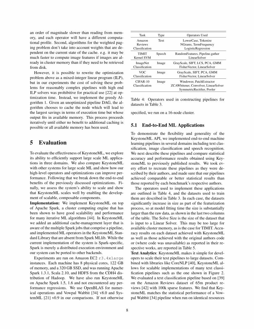
Task Type Operators Used

Amazon Text LowerCase, TokenizeReviews NGrams, TermFrequency

Classification LogisticRegression

TIMIT Speech RandomFeatures, Pipeline.gatherKernel SVM LinearSolver

ImageNet Image GrayScale, SIFT, LCS, PCA, GMMClassification FisherVector, LinearSolver

VOC Image GrayScale, SIFT, PCA, GMMClassification FisherVector, LinearSolver

CIFAR-10 Image Windower, PatchExtractorClassification ZCAWhitener, Convolver, LinearSolver

SymmetricRectifier, Pooler

Table 4: Operators used in constructing pipelines fordatasets in Table 3.

specified, we run on a 16-node cluster.

5.1 End-to-End ML Applications

To demonstrate the flexibility and generality of theKeystoneML API, we implemented end-to-end machinelearning pipelines in several domains including text clas-sification, image classification and speech recognition.We next describe these pipelines and compare statisticalaccuracy and performance results obtained using Key-stoneML to previously published results. We took ev-ery effort to recreate these pipelines as they were de-scribed by their authors, and made sure that our pipelinesachieved comparable or better statistical results thanthose reported by each benchmark’s respective authors.

The operators used to implement these applicationsare outlined in Table 4, and the datasets used to trainthem are described in Table 3. In each case, the datasetssignificantly increase in size as part of the featurizationprocess, so at model fitting time the size is substantiallylarger than the raw data, as shown in the last two columnsof the table. The Solve Size is the size of the dataset thatis input to a Linear Solver. This may be too large foravailable cluster memory, as is the case for TIMIT. Accu-racy results on each dataset achieved with KeystoneMLas well as those achieved with the original authors codeor (where code was unavailable) as reported in their re-spective works, are reported in Table 5.Text Analytics: KeystoneML makes it simple for devel-opers to scale their text pipelines to large datasets. Com-bined with libraries like CoreNLP [40], KeystoneML al-lows for scalable implementations of many text classi-fication pipelines such as the one shown in Figure 2.We evaluated a text classification pipeline based on [39]on the Amazon Reviews dataset of 65m product re-views [42] with 100k sparse features. We find that Key-stoneML matches the statistical performance of a Vow-pal Wabbit [34] pipeline when run on identical resources

8

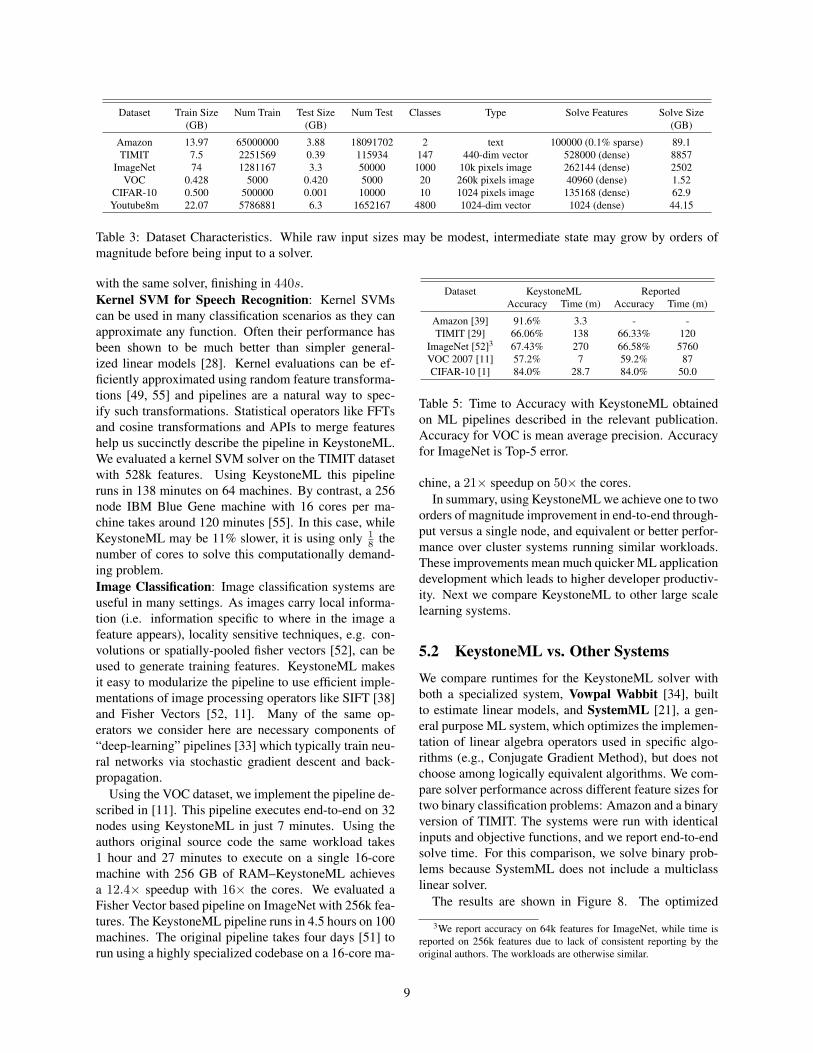
Dataset Train Size Num Train Test Size Num Test Classes Type Solve Features Solve Size(GB) (GB) (GB)

Amazon 13.97 65000000 3.88 18091702 2 text 100000 (0.1% sparse) 89.1TIMIT 7.5 2251569 0.39 115934 147 440-dim vector 528000 (dense) 8857

ImageNet 74 1281167 3.3 50000 1000 10k pixels image 262144 (dense) 2502VOC 0.428 5000 0.420 5000 20 260k pixels image 40960 (dense) 1.52

CIFAR-10 0.500 500000 0.001 10000 10 1024 pixels image 135168 (dense) 62.9Youtube8m 22.07 5786881 6.3 1652167 4800 1024-dim vector 1024 (dense) 44.15

Table 3: Dataset Characteristics. While raw input sizes may be modest, intermediate state may grow by orders ofmagnitude before being input to a solver.

with the same solver, finishing in 440s.Kernel SVM for Speech Recognition: Kernel SVMscan be used in many classification scenarios as they canapproximate any function. Often their performance hasbeen shown to be much better than simpler general-ized linear models [28]. Kernel evaluations can be ef-ficiently approximated using random feature transforma-tions [49, 55] and pipelines are a natural way to spec-ify such transformations. Statistical operators like FFTsand cosine transformations and APIs to merge featureshelp us succinctly describe the pipeline in KeystoneML.We evaluated a kernel SVM solver on the TIMIT datasetwith 528k features. Using KeystoneML this pipelineruns in 138 minutes on 64 machines. By contrast, a 256node IBM Blue Gene machine with 16 cores per ma-chine takes around 120 minutes [55]. In this case, whileKeystoneML may be 11% slower, it is using only 1

8 thenumber of cores to solve this computationally demand-ing problem.Image Classification: Image classification systems areuseful in many settings. As images carry local informa-tion (i.e. information specific to where in the image afeature appears), locality sensitive techniques, e.g. con-volutions or spatially-pooled fisher vectors [52], can beused to generate training features. KeystoneML makesit easy to modularize the pipeline to use efficient imple-mentations of image processing operators like SIFT [38]and Fisher Vectors [52, 11]. Many of the same op-erators we consider here are necessary components of“deep-learning” pipelines [33] which typically train neu-ral networks via stochastic gradient descent and back-propagation.

Using the VOC dataset, we implement the pipeline de-scribed in [11]. This pipeline executes end-to-end on 32nodes using KeystoneML in just 7 minutes. Using theauthors original source code the same workload takes1 hour and 27 minutes to execute on a single 16-coremachine with 256 GB of RAM–KeystoneML achievesa 12.4× speedup with 16× the cores. We evaluated aFisher Vector based pipeline on ImageNet with 256k fea-tures. The KeystoneML pipeline runs in 4.5 hours on 100machines. The original pipeline takes four days [51] torun using a highly specialized codebase on a 16-core ma-

Dataset KeystoneML ReportedAccuracy Time (m) Accuracy Time (m)

Amazon [39] 91.6% 3.3 - -TIMIT [29] 66.06% 138 66.33% 120

ImageNet [52]3 67.43% 270 66.58% 5760VOC 2007 [11] 57.2% 7 59.2% 87CIFAR-10 [1] 84.0% 28.7 84.0% 50.0

Table 5: Time to Accuracy with KeystoneML obtainedon ML pipelines described in the relevant publication.Accuracy for VOC is mean average precision. Accuracyfor ImageNet is Top-5 error.

chine, a 21× speedup on 50× the cores.In summary, using KeystoneML we achieve one to two

orders of magnitude improvement in end-to-end through-put versus a single node, and equivalent or better perfor-mance over cluster systems running similar workloads.These improvements mean much quicker ML applicationdevelopment which leads to higher developer productiv-ity. Next we compare KeystoneML to other large scalelearning systems.

5.2 KeystoneML vs. Other Systems

We compare runtimes for the KeystoneML solver withboth a specialized system, Vowpal Wabbit [34], builtto estimate linear models, and SystemML [21], a gen-eral purpose ML system, which optimizes the implemen-tation of linear algebra operators used in specific algo-rithms (e.g., Conjugate Gradient Method), but does notchoose among logically equivalent algorithms. We com-pare solver performance across different feature sizes fortwo binary classification problems: Amazon and a binaryversion of TIMIT. The systems were run with identicalinputs and objective functions, and we report end-to-endsolve time. For this comparison, we solve binary prob-lems because SystemML does not include a multiclasslinear solver.

The results are shown in Figure 8. The optimized

3We report accuracy on 64k features for ImageNet, while time isreported on 256k features due to lack of consistent reporting by theoriginal authors. The workloads are otherwise similar.

9

Amazon Binary TIMIT

1030

100300

1000

1024 2048 4096 8192 16384 1024 2048 4096 8192 16384Features

Tim

e (s

)

System KeystoneML Vowpal Wabbit SystemML

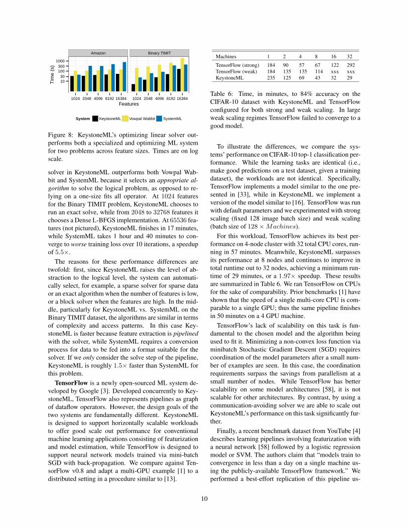
Figure 8: KeystoneML’s optimizing linear solver out-performs both a specialized and optimizing ML systemfor two problems across feature sizes. Times are on logscale.

solver in KeystoneML outperforms both Vowpal Wab-bit and SystemML because it selects an appropriate al-gorithm to solve the logical problem, as opposed to re-lying on a one-size fits all operator. At 1024 featuresfor the Binary TIMIT problem, KeystoneML chooses torun an exact solve, while from 2048 to 32768 features itchooses a Dense L-BFGS implementation. At 65536 fea-tures (not pictured), KeystoneML finishes in 17 minutes,while SystemML takes 1 hour and 40 minutes to con-verge to worse training loss over 10 iterations, a speedupof 5.5×.

The reasons for these performance differences aretwofold: first, since KeystoneML raises the level of ab-straction to the logical level, the system can automati-cally select, for example, a sparse solver for sparse dataor an exact algorithm when the number of features is low,or a block solver when the features are high. In the mid-dle, particularly for KeystoneML vs. SystemML on theBinary TIMIT dataset, the algorithms are similar in termsof complexity and access patterns. In this case Key-stoneML is faster because feature extraction is pipelinedwith the solver, while SystemML requires a conversionprocess for data to be fed into a format suitable for thesolver. If we only consider the solve step of the pipeline,KeystoneML is roughly 1.5× faster than SystemML forthis problem.

TensorFlow is a newly open-sourced ML system de-veloped by Google [3]. Developed concurrently to Key-stoneML, TensorFlow also represents pipelines as graphof dataflow operators. However, the design goals of thetwo systems are fundamentally different. KeystoneMLis designed to support horizontally scalable workloadsto offer good scale out performance for conventionalmachine learning applications consisting of featurizationand model estimation, while TensorFlow is designed tosupport neural network models trained via mini-batchSGD with back-propagation. We compare against Ten-sorFlow v0.8 and adapt a multi-GPU example [1] to adistributed setting in a procedure similar to [13].

Machines 1 2 4 8 16 32

TensorFlow (strong) 184 90 57 67 122 292TensorFlow (weak) 184 135 135 114 xxx xxxKeystoneML 235 125 69 43 32 29

Table 6: Time, in minutes, to 84% accuracy on theCIFAR-10 dataset with KeystoneML and TensorFlowconfigured for both strong and weak scaling. In largeweak scaling regimes TensorFlow failed to converge to agood model.

To illustrate the differences, we compare the sys-tems’ performance on CIFAR-10 top-1 classification per-formance. While the learning tasks are identical (i.e.,make good predictions on a test dataset, given a trainingdataset), the workloads are not identical. Specifically,TensorFlow implements a model similar to the one pre-sented in [33], while in KeystoneML we implement aversion of the model similar to [16]. TensorFlow was runwith default parameters and we experimented with strongscaling (fixed 128 image batch size) and weak scaling(batch size of 128×Machines).

For this workload, TensorFlow achieves its best per-formance on 4-node cluster with 32 total CPU cores, run-ning in 57 minutes. Meanwhile, KeystoneML surpassesits performance at 8 nodes and continues to improve intotal runtime out to 32 nodes, achieving a minimum run-time of 29 minutes, or a 1.97× speedup. These resultsare summarized in Table 6. We ran TensorFlow on CPUsfor the sake of comparability. Prior benchmarks [1] haveshown that the speed of a single multi-core CPU is com-parable to a single GPU; thus the same pipeline finishesin 50 minutes on a 4 GPU machine.

TensorFlow’s lack of scalability on this task is fun-damental to the chosen model and the algorithm beingused to fit it. Minimizing a non-convex loss function viaminibatch Stochastic Gradient Descent (SGD) requirescoordination of the model parameters after a small num-ber of examples are seen. In this case, the coordinationrequirements surpass the savings from parallelism at asmall number of nodes. While TensorFlow has betterscalability on some model architectures [58], it is notscalable for other architectures. By contrast, by using acommunication-avoiding solver we are able to scale outKeystoneML’s performance on this task significantly fur-ther.

Finally, a recent benchmark dataset from YouTube [4]describes learning pipelines involving featurization witha neural network [58] followed by a logistic regressionmodel or SVM. The authors claim that “models train toconvergence in less than a day on a single machine us-ing the publicly-available TensorFlow framework.” Weperformed a best-effort replication of this pipeline us-

10

KeystoneML

Pipe Only

None

KeystoneML

Pipe Only

None

KeystoneML

Pipe Only

None

Am

azonT

imit

VO

C

0 2000 4000 6000

Duration (s)

Opt

imiz

atio

n Le

vel

Stage Optimize Featurize Solve Eval

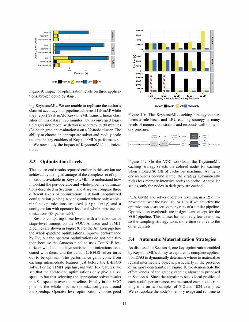
Figure 9: Impact of optimization levels on three applica-tions, broken down by stage.

ing KeystoneML. We are unable to replicate the author’sclaimed accuracy–our pipeline achieves 21% mAP whilethey report 28% mAP. KeystoneML trains a linear clas-sifier on this dataset in 3 minutes, and a converged logis-tic regression model with worse accuracy in 90 minutes(31 batch gradient evaluations) on a 32-node cluster. Theability to choose an appropriate solver and readily scaleout are the key enablers of KeystoneML’s performance.

We now study the impact of KeystoneML’s optimiza-tions.

5.3 Optimization LevelsThe end-to-end results reported earlier in this section areachieved by taking advantage of the complete set of opti-mizations available in KeystoneML. To understand howimportant the per-operator and whole-pipeline optimiza-tions described in Sections 3 and 4 are we compare threedifferent levels of optimization: a default unoptimizedconfiguration (None), a configuration where only whole-pipeline optimizations are used (Pipe Only) and aconfiguration with operator-level and whole-pipeline op-timizations (KeystoneML).

Results comparing these levels, with a breakdown ofstage-level timings on the VOC, Amazon and TIMITpipelines are shown in Figure 9. For the Amazon pipelinethe whole-pipeline optimizations improve performanceby 7×, but the operator optimizations do not help fur-ther, because the Amazon pipeline uses CoreNLP fea-turizers which do not have statistical optimizations asso-ciated with them, and the default L-BFGS solver turnsout to be optimal. The performance gains come fromcaching intermediate features just before the L-BFGSsolve. For the TIMIT pipeline, run with 16k features, wesee that the end-to-end optimizations only give a 1.3×speedup but that selecting the appropriate solver resultsin a 8× speedup over the baseline. Finally in the VOCpipeline the whole pipeline optimization gives around3× speedup. Operator-level optimization chooses good

Figure 10: The KeystoneML caching strategy outper-forms a rule-based and LRU caching strategy at manylevels of memory constraints and responds well to mem-ory pressure.

Training Data Grayscaler SIFT Extractor

Reduce Dimensions

Fisher Vector Normalize

Column Sampler

Linear Map

PCA Column Sampler GMM Linear

Solver

Predictions

Training Labels

Figure 11: On the VOC workload, the KeystoneMLcaching strategy selects the colored nodes for cachingwhen allotted 80 GB of cache per machine. As mem-ory resources become scarce, the strategy automaticallypicks less memory intensive nodes to cache. At smallerscales, only the nodes in dark gray are cached.

PCA, GMM and solver operators resulting in a 12× im-provement over the baseline, or 15× if we amortize theoptimization costs across many runs of a similar pipeline.Optimization overheads are insignificant except for theVOC pipeline. This dataset has relatively few examples,so the sampling strategy takes more time relative to theother datasets.

5.4 Automatic Materialization Strategies

As discussed in Section 4, one key optimization enabledby KeystoneML’s ability to capture the complete applica-tion DAG to dynamically determine where to materializereused intermediate objects, particularly in the presenceof memory constraints. In Figure 10 we demonstrate theeffectiveness of the greedy caching algorithm proposedin Section 4. Since the algorithm needs local profiles ofeach node’s performance, we measured each node’s run-ning time on two samples of 512 and 1024 examples.We extrapolate the node’s memory usage and runtime to

11

full scale using linear regression. We found that memoryestimates from this process are highly accurate and run-time estimates were within 15% of actual runtimes. Ifestimates are inaccurate, we fall back to an LRU replace-ment policy for the cache set determined by this proce-dure. While this measurement process is imperfect, it isadequate at identifying relative running times and thus issufficient for our purpose of resource management.

We compare this strategy with two alternatives–thefirst is a simple rule-based approach which only cachesthe results of Estimators. This is a sensible rule to follow,as the result of an Estimator (a Transformer or model) iscomputationally expensive to acquire and typically holdsa small memory footprint. However, this is not sufficientfor most practical pipelines because if a pipeline containsmore than one Estimator, often the input to the first Es-timator will be used downstream, thus presenting an op-portunity for reuse. The second approach is a Least Re-cently Used (LRU) policy: in a regime where memory isunconstrained, LRU matches the ideal strategy and fur-ther, LRU is the default memory management strategyused by Apache Spark. However, LRU does not take intoaccount that datasets from other jobs (even ones in thesame pipeline) are vying for presence in cluster memory.

From Figure 10 we notice several important trends.First, the KeystoneML strategy is nearly always betterthan either of the other strategies. In the unconstrainedcase, the algorithm is going to remember all reused itemsas late in their journey through the pipeline as possible.In the constrained case, it will do as least as well as re-membering the (small) estimators which are by definitionreused later in the pipeline. Additionally, the strategy de-grades effectively, mixing between the best performanceof the limited-memory rule-based strategy and the LRUbased “cache everything” strategy which works well inunconstrained settings. Curiously, as we increased thememory available to caching per-node, the LRU strategyperformed worse for the Amazon pipeline. Upon furtherinvestigation, this is because Spark has an implicit ad-mission control policy which only allows objects undersome proportion of the cache size to be admitted to thecache at runtime. As the cache size gets bigger in theLRU case, massive objects which are not then reused areadmitted to the cache and evict smaller objects which arereused and thus need to be recomputed.

To give a concrete example of the optimizer in action,consider the VOC pipeline (Figure 11). When mem-ory is not unconstrained (80 GB per node), the outputsfrom the SIFT, ReduceDimensions, Normalizeand TrainingLabels are cached. When memoryis restricted (5 GB per node) only the output fromNormalize and TrainingLabels are cached.

These results show that both per-operator and whole-pipeline optimizations are important for end-to-end per-

Amazon TIMIT ImageNet

0

5

10

15

0

20

40

60

0

100

200

300

400

500

8 16 32 64 128 8 16 32 64 128 8 16 32 64 128Cluster Size (# of nodes)

Tim

e (m

inut

es)

StageLoading Train Data Featurization Model Solve

Loading Test Data Model Eval

Figure 12: Time breakdown of workloads by stage. Thered line indicates ideal strong scaling performance over8 nodes.

formance improvements. We next study the scalabilityof the system on three workloads

5.5 Scalability

As discussed in previous sections, KeystoneML’s APIdesign encourages the construction of scalable operators.However, some estimators like linear solvers need co-ordination [18] among workers to compute correct re-sults. In Figure 12 we demonstrate the scaling propertiesfrom 8 to 128 nodes of the text, image, and Kernel SVMpipelines on the Amazon, ImageNet (with 16k features)and TIMIT datasets (with 65k features) respectively. TheImageNet pipeline exhibits near-perfect horizontal scal-ability up to 128 nodes, while the Amazon and TIMITpipeline scale well up to 64 nodes.

To understand why the Amazon and TIMIT pipelinedo not scale linearly to 128 nodes, we further analyze thebreakdown of time take by each stage. We see that eachpipeline is dominated by a different part of its computa-tion. The TIMIT pipeline is dominated by its solve stage,while featurization dominates the Amazon and ImageNetpipelines. Scaling linear solvers is known to require co-ordination [18], which leads directly to sub-linear scal-ability of the whole pipeline. Similarly, in the Amazonpipeline, one of the featurization steps uses an aggrega-tion tree which does not scale linearly.

6 Related WorkML Frameworks: ML researchers have traditionallyused MATLAB or R packages to develop ML routines.The importance of feature engineering has led to toolslike scikit-learn [45] and KNIME [8] adding supportfor featurization for small datasets. Further, existing li-braries for large scale ML [10] like Vowpal Wabbit [34],GraphLab [37], MLlib [44], RIOT [62], DimmWit-ted [61] focus on efficient implementations of learningalgorithms like regression, classification and linear alge-

12

bra routines. In KeystoneML, we focus on pipelines thatinclude featurization and show how to optimize perfor-mance with end-to-end information. Work in ParameterServers [36] has studied how to share model updates. InKeystoneML we implement a high-level API for linearsolvers and can leverage parameter servers in our archi-tecture.

Closely related to KeystoneML is SystemML [21]which also uses an optimization based approach to deter-mine the physical execution strategy of ML algorithms.However, SystemML places less emphasis on support forUDFs and featurization, while instead focusing on linearalgebra operators which have well specified semantics.To handle featurization we develop an extensible API inKeystoneML which allows for cost profiling of arbitrarynodes and uses these cost estimates to make node-leveland whole-pipeline optimizations. Other work [60, 5]has looked at optimizing caching strategies and operatorselection in the regime of feature selection and featuregeneration workloads. KeystoneML considers similarproblems in the context of distributed ML operators andend-to-end learning pipelines. Developed concurrentlyto KeystoneML is TensorFlow [3]. While designed tosupport different learning workloads the optimizationsthat are a part of KeystoneML can also be applied to sys-tems like TensorFlow.

Projects such as Bismarck [20], MADLib [27], andGLADE [47] have proposed techniques to integrate MLalgorithms inside database engines. In KeystoneML, wedevelop a high level API and show how we can achievesimilar benefits of modularity and end-to-end optimiza-tion while also being scalable. These systems do notpresent cross-operator optimizations and do not considertradeoffs at the operator level that we consider in Key-stoneML. Finally, Spark ML [43] represents an early de-sign of a similar high-level API for machine learning.We present a type safe API and optimization frameworkfor such a system. The version we present in this pa-per differs in its use of type-safe operations, support forcomplex data flows, internal DAG representation and op-timizations discussed in Sections 3 and 4. Finally, theconcept of using a high-level programming model hasbeen explored in a number of other contexts, includingcompilers [35] and networking [31]. In this paper wefocus on machine learning workloads and propose node-level and end-to-end optimizations.Query Optimization, Modular Design, Caching:There are several similarities between the optimizationsmade by KeystoneML and traditional relational queryoptimizers. Even the earliest relational query opti-mizers [54] used multiple physical implementations ofequivalent logical operators, and like many relational op-timizers, the KeystoneML optimizer is cost-based. How-ever, KeystoneML supports a much richer set of data

types than a traditional relational query system, and ouroperators lack some relational algebra semantics, such ascommutativity, limiting the system’s ability to performcertain optimizations. Further, KeystoneML switchesamong operators that provide exact answers vs approxi-mate ones to save time due to the workload setting. Datacharacteristics such as sparsity are not traditionally con-sidered by optimizers.

The caching strategy employed by KeystoneML canbe viewed as a form of view selection for material-ized view maintenance over queries with expensive user-defined functions [15, 26], we focus on materializationfor intra-query optimization, as opposed to inter-queryoptimization [25, 12, 63, 19, 46]. While much of therelated work focuses on the challenging problem of viewmaintenance in the presence of updates, KeystoneML weexploit the iterative nature and immutable properties ofthis state.

7 Future Work and Conclusion

KeystoneML represents a significant first step towardseasy-to-use, robust, and efficient end-to-end ML at mas-sive scale. We plan to investigate pipeline optimiza-tions like node reordering to reduce data transfers andalso look at how hyperparameter tuning [56] can be inte-grated into the system. The existing KeystoneML oper-ator APIs are synchronous and our existing pipelines areacyclic. In the future we plan to study how algorithmslike asynchronous SGD [36] or back-propagation can beintegrated with the robustness and scalability that Key-stoneML provides.

We have presented the design of KeystoneML, asystem that enables the development end-to-end MLpipelines. By capturing the end-to-end application, Key-stoneML can automatically optimize execution at boththe operator and whole-pipeline levels, enabling solu-tions that automatically adapt to changes in data, hard-ware, and other environmental characteristics.Acknowledgements: We would like to thank XiangruiMeng, Joseph Bradley for their help in design discus-sions and Henry Milner, Daniel Brucker, Gylfi Gud-mundsson, Zongheng Yang, Vaishaal Shankar for theircontributions to the KeystoneML source code. We wouldalso like to thank Peter Alvaro, Peter Bailis, Joseph Gon-zales, Nick Lanham, Aurojit Panda, Ameet Talwarkar fortheir feedback on earlier versions of this paper. Thisresearch is supported in part by NSF CISE Expedi-tions Award CCF-1139158, DOE Award SN10040 de-sc0012463, and DARPA XData Award FA8750-12-2-0331, and gifts from Amazon Web Services, Google,IBM, SAP, The Thomas and Stacey Siebel Foundation,Adatao, Adobe, Apple, Inc., Blue Goji, Bosch, Cisco,

13

Cray, Cloudera, EMC2, Ericsson, Facebook, Guavus,HP, Huawei, Informatica, Intel, Microsoft, NetApp,Pivotal, Samsung, Schlumberger, Splunk, Virdata andVMware.

References[1] TensorFlow CIFAR-10 Performance as reported in Ten-

sorFlow Source Code. https://git.io/v2b4J.

[2] ENCODE-DREAM in vivo Transcription Factor BindingSite Prediction Challenge. https://www.synapse.org/#!Synapse:syn6131484, 2016.

[3] M. Abadi, A. Agarwal, P. Barham, E. Brevdo, et al. Ten-sorFlow: Large-scale machine learning on heterogeneoussystems, 2015. Software available from tensorflow.org.

[4] S. Abu-El-Haija, N. Kothari, J. Lee, P. Natsev, et al.YouTube-8M: A Large-Scale Video Classification Bench-mark. arXiv preprint arXiv: 1609.08675, 2016.

[5] F. Abuzaid, S. Hadjis, C. Zhang, and C. Re. Caffe conTroll: Shallow Ideas to Speed Up Deep Learning. CoRRabs/1504.04343, 2015.

[6] G. M. Ballard. Avoiding Communication in Dense LinearAlgebra. PhD thesis, University of California, Berkeley,2013.

[7] L. A. Belady. A study of replacement algorithms for avirtual-storage computer. IBM Systems journal, 5(2):78–101, 1966.

[8] M. R. Berthold, N. Cebron, F. Dill, T. R. Gabriel, et al.KNIME: The Konstanz information miner. In Data anal-ysis, machine learning and applications, pages 319–326.Springer, 2008.

[9] D. P. Bertsekas and J. N. Tsitsiklis. Parallel and dis-tributed computation: numerical methods. Prentice-Hall,Inc., 1989.

[10] Z. Cai, Z. J. Gao, S. Luo, L. L. Perez, et al. A compari-son of platforms for implementing and running very largescale machine learning algorithms. In SIGMOD 2014,pages 1371–1382, 2014.

[11] K. Chatfield, V. Lempitsky, A. Vedaldi, and A. Zisserman.The devil is in the details: an evaluation of recent featureencoding methods. In British Machine Vision Conference,2011.

[12] S. Chaudhuri and V. R. Narasayya. AutoAdmin ’What-if’Index Analysis Utility. SIGMOD, 1998.

[13] J. Chen, R. Monga, S. Bengio, and R. Jozefowicz. Re-visiting distributed synchronous sgd. arXiv preprintarxiv:1604.00981, 2016.

[14] W. Chen, Z. Wang, and J. Zhou. Large-scale l-bfgs usingmapreduce. In NIPS, pages 1332–1340, 2014.

[15] R. Chirkova and J. Yang. Materialized Views. Founda-tions and Trends in Databases, 2012.

[16] A. Coates and A. Y. Ng. Learning Feature Representa-tions with K-Means. In Neural Networks: Tricks of theTrade. 2012.

[17] A. Crotty, A. Galakatos, and T. Kraska. Tupleware: Dis-tributed machine learning on small clusters. IEEE DataEng. Bull, 37(3), 2014.

[18] J. Demmel, L. Grigori, M. Hoemmen, and J. Langou.Communication-optimal parallel and sequential QR andLU factorizations. SIAM Journal on Scientific Comput-ing, 34(1):A206–A239, 2012.

[19] I. Elghandour and A. Aboulnaga. ReStore: reusing resultsof MapReduce jobs. In PVLDB, 2012.

[20] X. Feng, A. Kumar, B. Recht, and C. Re. Towards aunified architecture for in-rdbms analytics. In SIGMOD,2012.

[21] A. Ghoting, R. Krishnamurthy, E. Pednault, B. Rein-wald, et al. SystemML: Declarative machine learning onMapReduce. In ICDE, pages 231–242. IEEE, 2011.

[22] I. Gurobi Optimization. Gurobi optimizer reference man-ual, 2015.

[23] A. Halevy, P. Norvig, and F. Pereira. The unreasonableeffectiveness of data. Intelligent Systems, IEEE, 24(2):8–12, 2009.

[24] N. Halko, P. G. Martinsson, and J. A. Tropp. Find-ing Structure with Randomness: Probabilistic Algorithmsfor Constructing Approximate Matrix Decompositions.SIAM Review, 2011.

[25] V. Harinarayan, A. Rajaraman, and J. D. Ullman. Imple-menting Data Cubes Efficiently. SIGMOD, pages 205–216, 1996.

[26] J. M. Hellerstein and J. F. Naughton. Query executiontechniques for caching expensive methods. SIGMOD,1997.

[27] J. M. Hellerstein, C. Re, F. Schoppmann, D. Z. Wang,et al. The MADlib analytics library: or MAD skills, theSQL. PVLDB, 5(12):1700–1711, 2012.

[28] C.-W. Hsu, C.-C. Chang, C.-J. Lin, et al. A practicalguide to support vector classification. https://goo.gl/m68USr, 2003.

[29] P.-S. Huang, H. Avron, T. N. Sainath, V. Sindhwani, andB. Ramabhadran. Kernel methods match deep neural net-works on timit. In ICASSP, pages 205–209. IEEE, 2014.

[30] E. Jonas, V. Shankar, M. Bobra, and B. Recht. Flare pre-diction using photospheric and coronal image data. AGUFall Meeting, 2016.

[31] E. Kohler, R. Morris, B. Chen, J. Jannotti, and M. F.Kaashoek. The Click modular router. ACM Transactionson Computer Systems (TOCS), 2000.

[32] T. Kraska, A. Talwalkar, J. C. Duchi, R. Griffith, et al.MLbase: A Distributed Machine-learning System. CIDR,2013.

[33] A. Krizhevsky and G. Hinton. Convolutional Deep BeliefNetworks on CIFAR-10. Unpublished manuscript, 2010.

[34] J. Langford, L. Li, and A. Strehl. Vowpal wabbit onlinelearning project, 2007.

14

[35] C. Lattner and V. Adve. LLVM: A Compilation Frame-work for Lifelong Program Analysis & Transformation.In CGO, 2004.

[36] M. Li, D. G. Andersen, J. W. Park, A. J. Smola, et al.Scaling Distributed Machine Learning with the ParameterServer. OSDI, 2014.

[37] Y. Low, D. Bickson, J. Gonzalez, C. Guestrin, et al. Dis-tributed graphlab: a framework for machine learning anddata mining in the cloud. PVLDB, 5(8):716–727, 2012.

[38] D. G. Lowe. Object recognition from local scale-invariantfeatures. In ICCV, volume 2, pages 1150–1157. IEEE,1999.

[39] C. Manning and D. Klein. Optimization, maxent mod-els, and conditional estimation without magic. In HLT-NAACL, Tutorial Vol 5, 2003.

[40] C. D. Manning, M. Surdeanu, J. Bauer, J. Finkel,et al. The Stanford CoreNLP natural language process-ing toolkit. In ACL, 2014.

[41] M. Mathieu, M. Henaff, and Y. LeCun. Fast Training ofConvolutional Networks through FFTs. ICLR, 2014.

[42] J. McAuley, R. Pandey, and J. Leskovec. Inferring net-works of substitutable and complementary products. InKDD, pages 785–794, 2015.

[43] X. Meng, J. Bradley, E. Sparks, and S. Venkataraman. MLPipelines: A New High-Level API for MLlib. https://goo.gl/pluhq0, 2015.

[44] X. Meng, J. K. Bradley, B. Yavuz, E. R. Sparks, et al.MLlib: Machine Learning in Apache Spark. CoRR,abs/1505.06807, 2015.

[45] F. Pedregosa, G. Varoquaux, A. Gramfort, et al. Scikit-learn: Machine learning in Python. JMLR, 12:2825–2830, 2011.

[46] L. Perez and C. Jermaine. History-aware query opti-mization with materialized intermediate views. In ICDE,pages 520–531, March 2014.

[47] C. Qin and F. Rusu. Scalable I/O-bound Parallel In-cremental Gradient Descent for Big Data Analytics inGLADE. In DanaC, 2013.

[48] P. Raghavan and M. Snir. Memory versus randomizationin on-line algorithms. In International Colloquium on Au-tomata, Languages, and Programming, pages 687–703.Springer, 1989.

[49] A. Rahimi and B. Recht. Random features for large-scalekernel machines. In NIPS, pages 1177–1184, 2007.

[50] B. Recht, C. Re, S. Wright, and F. Niu. Hogwild!: A lock-free approach to parallelizing stochastic gradient descent.In NIPS, pages 693–701, 2011.

[51] J. Sanchez, F. Perronnin, and T. Mensink. Im-proved fisher vector for large scale image classifi-cation. http://image-net.org/challenges/LSVRC/2010/ILSVRC2010_XRCE.pdf.

[52] J. Sanchez, F. Perronnin, T. Mensink, and J. Verbeek.Image classification with the fisher vector: Theory andpractice. International journal of computer vision,105(3):222–245, 2013.

[53] D. Sculley, G. Holt, D. Golovin, E. Davydov, T. Phillips,D. Ebner, V. Chaudhary, and M. Young. Machine learn-ing: The high interest credit card of technical debt.In SE4ML: Software Engineering for Machine Learning(NIPS 2014 Workshop), 2014.

[54] P. G. Selinger, M. M. Astrahan, D. D. Chamberlin, R. A.Lorie, and T. G. Price. Access path selection in a re-lational database management system. SIGMOD, pages141–152, Aug. 1979.

[55] V. Sindhwani and H. Avron. High-performance kernelmachines with implicit distributed optimization and ran-domization. CoRR, abs/1409.0940, 2014.

[56] E. R. Sparks, A. Talwalkar, D. Haas, M. J. Franklin, et al.Automating model search for large scale machine learn-ing. In SoCC ’15, 2015.

[57] M. Stonebraker, J. Becla, D. J. DeWitt, K.-T. Lim,D. Maier, O. Ratzesberger, and S. B. Zdonik. Require-ments for science data bases and scidb. In CIDR, vol-ume 7, pages 173–184, 2009.

[58] C. Szegedy, V. Vanhoucke, et al. Rethinking the in-ception architecture for computer vision. arXiv preprintarXiv:1512.00567, 2015.

[59] S. Williams, A. Waterman, and D. Patterson. Roofline:An Insightful Visual Performance Model for MulticoreArchitectures. CACM, 2009.

[60] C. Zhang, A. Kumar, and C. Re. Materialization opti-mizations for feature selection workloads. In SIGMOD,2014.

[61] C. Zhang and C. Re. Dimmwitted: A study of main-memory statistical analytics. PVLDB, 7(12):1283–1294,2014.

[62] Y. Zhang, H. Herodotou, and J. Yang. RIOT: I/O-EfficientNumerical Computing without SQL. In CIDR, 2009.

[63] D. C. Zilio, C. Zuzarte, G. M. Lohman, H. Pirahesh,et al. Recommending Materialized Views and Indexeswith IBM DB2 Design Advisor. In ICAC 2004, May2004.

15