Human contribution to the record-breaking July 2019 heat wave in

Western Europe

Robert Vautard, Olivier Boucher (IPSL Paris)

Geert Jan van Oldenborgh (KNMI)

Friederike Otto, Karsten Haustein (University of Oxford)

Martha M. Vogel, Sonia I. Seneviratne (ETH Zürich)

Jean-Michel Soubeyroux, Michel Schneider, Agathe Drouin, Aurélien Ribes (Météo France)

Frank Kreienkamp (Deutscher Wetterdienst)

Peter Stott (UK Met Office)

Maarten van Aalst (ITC/University of Twente and Red Cross Red Crescent Climate Centre)

Key findings

● A second record-breaking heat wave of 3-4 days took place in Western Europe

in the last week of July 2019, with temperatures exceeding 40 degrees in many

countries including Belgium and the Netherlands where temperatures above

40°C were recorded for the first time. In the U.K. the event was shorter lived (1-

2 days), yet a new historical daily maximum temperature was recorded

exceeding the previous record set during the hazardous August 2003

heatwave.

● In contrast to other heat waves that have been attributed in Western Europe

before, this July heat was also a rare event in today’s climate in France and the

Netherlands. There, the observed temperatures, averaged over 3 days, were

estimated to have a 50-year to 150-year return period in the current climate.

Note that return periods of temperatures vary between different measures and

locations, and are therefore highly uncertain.

● Combining information from models and observations, we find that such

heatwaves in France and the Netherlands would have had return periods that

are about a hundred times higher (at least 10 times) without climate change.

Over France and the Netherlands, such temperatures would have had

extremely little chance to occur without human influence on climate (return

periods higher than ~1000 years).

● In the U.K. and Germany, the event is less rare (estimated return periods

around 10-30 years in the current climate) and the likelihood is about 10 times

higher (at least 3 times) due to climate change. Such an event would have had

return periods of from a few tens to a few hundreds of years without climate

change.

● In all locations an event like the observed would have been 1.5 to 3 ºC cooler in

an unchanged climate.

● As for the June heatwave, we found that climate models have systematic

biases in representing heat waves at these time scales and they show about

50% smaller trends than observations in this part of Europe and much higher

year-to-year variability than the observations. Despite this, models still

simulate very large probability changes.

● Heatwaves during the height of summer pose a substantial risk to human

health and are potentially lethal. This risk is aggravated by climate change, but

also by other factors such as an aging population, urbanisation, changing

social structures, and levels of preparedness. The full impact is only known

after a few weeks when the mortality figures have been analysed. Effective heat

emergency plans, together with accurate weather forecasts such as those

issued before this heatwave, reduce impacts and are becoming even more

important in light of the rising risks.

● It is noteworthy that every heatwave analysed so far in Europe in recent years

(2003, 2010, 2015, 2017, 2018, June 2019 and this study) was found to be made

much more likely and more intense due to human-induced climate change.

How much more depends very strongly on the event definition: location,

season, intensity and durations. The July 2019 heatwave was so extreme over

continental Western Europe that the observed magnitudes would have been

extremely unlikely without climate change.

Introduction, Trigger

After the extreme heat that took place in the last week of June 2019, a second record-breaking

heatwave struck Western Europe and Scandinavia at the end of July 2019. In June, new all-time

records were set in multiple places across Western Europe. In July, records were broken again, albeit

in different areas. Taking into account both episodes, the spatial extent of broken historical records is

large: in most areas of France, the Benelux, Switzerland, in western Germany, Eastern U.K. and

Northern Italy. Some of these previous records were set as early as the 1950s, with some stations

setting new records that have continuously been monitoring the weather for more than 200 years (e.g.

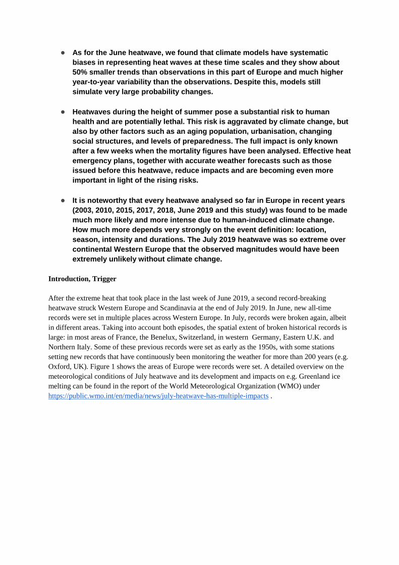
Oxford, UK). Figure 1 shows the areas of Europe were records were set. A detailed overview on the

meteorological conditions of July heatwave and its development and impacts on e.g. Greenland ice

melting can be found in the report of the World Meteorological Organization (WMO) under

https://public.wmo.int/en/media/news/july-heatwave-has-multiple-impacts .

Figure 1: Rank of annual maximum temperatures observed in Europe in 2019 compared to 1950 -

2018, based on the E-OBS data set (Haylock et al., 2008, version 19, extended with monthly and daily

updates to 30 July 2019). This figure is made with preliminary data and should be taken with caution

as some measurements are not yet validated.

The July episode was rather short and intense, with about four days of very high temperatures. In

France, the highest amplitudes of the heatwave were found in Northern and Central parts of the

country, with records of either 1947 or 2003 broken by a large departure on 25 July. For instance, the

historical record of Paris (Station Paris-Montsouris) of 40.4°C became 42.6°C and a temperature of

43.6°C was measured in Saint Maur des Fossés a few kilometers away from Paris city in a residential

area. In Belgium and the Netherlands for the first time ever temperatures above 40°C were observed.

In Germany the historical record of 40.3 °C (in Kitzingen, 2015) has been surpassed by almost 1°C

(41.2°C at two stations) on 25 July, with one station reaching 42.6 °C (Lingen), which is thus the new

- officially confirmed - German temperature record. In total, the old record was exceeded at 15

stations in Germany. In the UK, a new highest ever maximum temperature of 38.7°C was measured in

Cambridge. Further west, where the heatwave was slightly less intense, the record from 1932 (35.1°C)

at the historic Oxford Radcliffe Meteorological Station (continuous measurements for more than 200

years) was broken by more than one degree, with the new record maximum temperature of 36.5°C.

While the new records made headlines, such extreme temperatures are dangerous, in particular when

prolonged over several days and nights. Heatwaves are known to increase mortality, especially among

those with existing respiratory illnesses and cardio-vascular disease, despite the fact that the

quantification of heat-related fatalities is not straightforward to assess and thus not known in near-real

time. However, compared to the 2003 heatwave, this time authorities were better prepared. Heatwave

action plans, aiming at preventing a catastrophic scenario such as in 2003, when more than 15,000

people died in France alone, are now in place. Preparedness was also facilitated by very accurate

weather forecasts from the national met services. Several European weather services have issued heat

warnings. For instance, the temperatures of 42-43°C in Paris were consistently forecast 3-4 days

ahead by Météo-France.

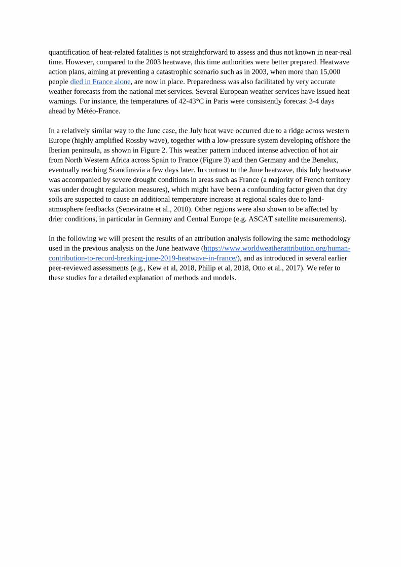
In a relatively similar way to the June case, the July heat wave occurred due to a ridge across western

Europe (highly amplified Rossby wave), together with a low-pressure system developing offshore the

Iberian peninsula, as shown in Figure 2. This weather pattern induced intense advection of hot air

from North Western Africa across Spain to France (Figure 3) and then Germany and the Benelux,

eventually reaching Scandinavia a few days later. In contrast to the June heatwave, this July heatwave

was accompanied by severe drought conditions in areas such as France (a majority of French territory

was under drought regulation measures), which might have been a confounding factor given that dry

soils are suspected to cause an additional temperature increase at regional scales due to land-

atmosphere feedbacks (Seneviratne et al., 2010). Other regions were also shown to be affected by

drier conditions, in particular in Germany and Central Europe (e.g. ASCAT satellite measurements).

In the following we will present the results of an attribution analysis following the same methodology

used in the previous analysis on the June heatwave (https://www.worldweatherattribution.org/human-

contribution-to-record-breaking-june-2019-heatwave-in-france/), and as introduced in several earlier

peer-reviewed assessments (e.g., Kew et al, 2018, Philip et al, 2018, Otto et al., 2017). We refer to

these studies for a detailed explanation of methods and models.

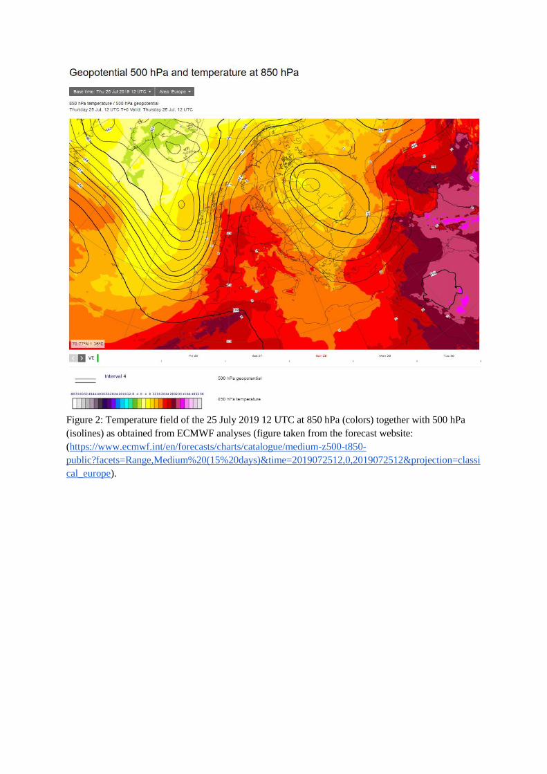
Figure 2: Temperature field of the 25 July 2019 12 UTC at 850 hPa (colors) together with 500 hPa

(isolines) as obtained from ECMWF analyses (figure taken from the forecast website:

(https://www.ecmwf.int/en/forecasts/charts/catalogue/medium-z500-t850-

public?facets=Range,Medium%20(15%20days)&time=2019072512,0,2019072512&projection=classi

cal_europe).

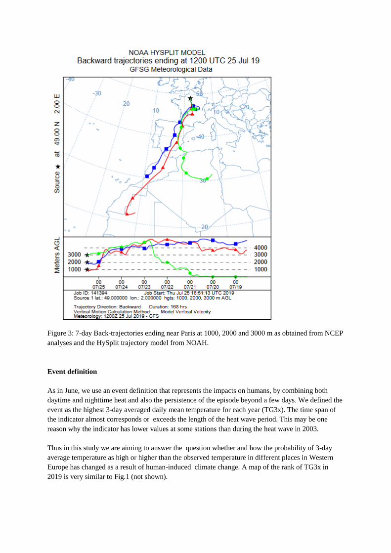
Figure 3: 7-day Back-trajectories ending near Paris at 1000, 2000 and 3000 m as obtained from NCEP

analyses and the HySplit trajectory model from NOAH.

Event definition

As in June, we use an event definition that represents the impacts on humans, by combining both

daytime and nighttime heat and also the persistence of the episode beyond a few days. We defined the

event as the highest 3-day averaged daily mean temperature for each year (TG3x). The time span of

the indicator almost corresponds or exceeds the length of the heat wave period. This may be one

reason why the indicator has lower values at some stations than during the heat wave in 2003.

Thus in this study we are aiming to answer the question whether and how the probability of 3-day

average temperature as high or higher than the observed temperature in different places in Western

Europe has changed as a result of human-induced climate change. A map of the rank of TG3x in

2019 is very similar to Fig.1 (not shown).

In order to give a flavour of how this heatwave was felt in different places in Europe, we selected

several locations in France, Germany, The Netherlands and the U.K.; countries in which a number of

temperature records were broken, and data were readily availability through study participants or

public websites.

The locations considered are shown in Table 1. The average over metropolitan France is close to the

value of the official French thermal index (used in the June heatwave study), which averages

temperature over 30 sites well distributed over the metropolitan area and is used to characterize heat

waves and cold spells at the scale of the country. The rest of the analysis is based on a set of 5

individual weather stations. We selected the stations based on the availability of data, their series

length (at least starting in 1951) and avoidance of urban heat island (UHI) and Irrigation Cooling

Effects (ICE), which result in non-climatic trends. The locations considered all witnessed a historical

record both in daily maximum and in 3-day mean temperature (apart from Oxford and Weilerswist-

Lommersum where only daily maximum temperatures set a record). Further, the selected stations are

either the nearest station with a long enough record to where the study authors reside, or representing

a national record. During the analysis we also gained access to the unreleased homogenised daily time

series from Uccle (Brussels). The trend in observations is very similar to Lille and De Bilt, but we

could not include it fully in the analysis.

Table 1: the locations considered for the event definition

Location Observation

source

Longitude Latitude Data start

France metropolitan

Average

E-OBS

Thermal index

1950

1947

Lille Lesquin (FR) ECA&D 3.15°E 50.97°N 1945

De Bilt (NL) KNMI 5.18°E 52.10°N 1901

Cambridge BG (UK) MOHC 0.13°E 52.19°N 1911

Oxford (UK) Univ Oxford -1.27°E 51.77°N 1815

Weilerswist-

Lommersum (DE)

DWD 6.79°E 50.71°N 1937

The De Bilt station has been statistically corrected for a change in hut from a pagoda to a Stevenson

screen in 1950 and a move from a sheltered garden to an open field in 1951.

The Cambridge Botanical Gardens (BG) station that observed the UK record temperature of 38.7 ºC

has a sizeable fraction of missing data. On 23 July there were battery issues, this value has been

estimated by the UK Met Office on the basis of their interpolation routine. For earlier years we used

the values of the nearby Cambridge NIAB station with a linear bias regression T(BG) = (1+A)

T(NIAB) + B, with A about 5% in summer and B -0.6 ºC in July, -0.9 ºC in August.

The German temperature was highest in Lingen, but there were debates about the validity of the

measured value. While it is now officially confirmed by the Deutscher Wetterdienst (DWD), here we

opted to analyse the nearby station Weilerswist-Lommersum. This rural station has observations

going back to 1937 with two years missing (December 1945 to November 1946 and September 2003

to July 2004). Yet the two hot summers of 1947 (TG3x 0.8 ºC cooler than 2019) and 2003 (TG3x 0.1

ºC hotter) are included.

Trend in observations

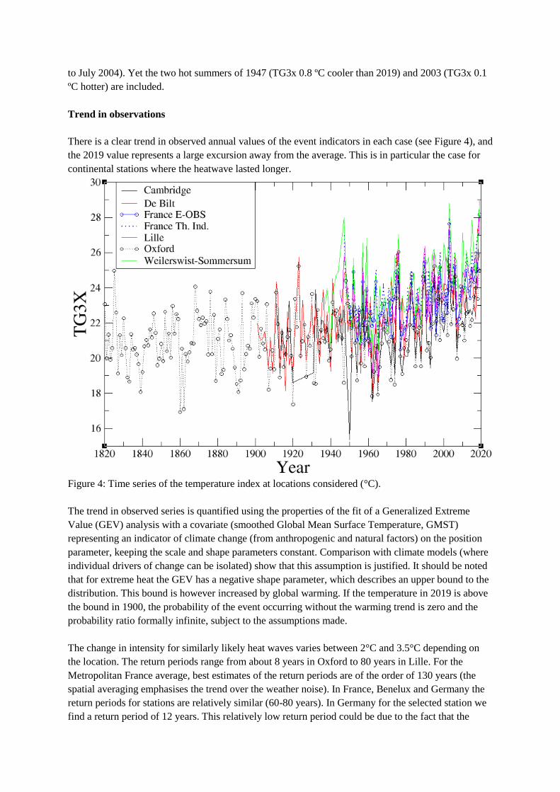
There is a clear trend in observed annual values of the event indicators in each case (see Figure 4), and

the 2019 value represents a large excursion away from the average. This is in particular the case for

continental stations where the heatwave lasted longer.

Figure 4: Time series of the temperature index at locations considered (°C).

The trend in observed series is quantified using the properties of the fit of a Generalized Extreme

Value (GEV) analysis with a covariate (smoothed Global Mean Surface Temperature, GMST)

representing an indicator of climate change (from anthropogenic and natural factors) on the position

parameter, keeping the scale and shape parameters constant. Comparison with climate models (where

individual drivers of change can be isolated) show that this assumption is justified. It should be noted

that for extreme heat the GEV has a negative shape parameter, which describes an upper bound to the

distribution. This bound is however increased by global warming. If the temperature in 2019 is above

the bound in 1900, the probability of the event occurring without the warming trend is zero and the

probability ratio formally infinite, subject to the assumptions made.

The change in intensity for similarly likely heat waves varies between 2°C and 3.5°C depending on

the location. The return periods range from about 8 years in Oxford to 80 years in Lille. For the

Metropolitan France average, best estimates of the return periods are of the order of 130 years (the

spatial averaging emphasises the trend over the weather noise). In France, Benelux and Germany the

return periods for stations are relatively similar (60-80 years). In Germany for the selected station we

find a return period of 12 years. This relatively low return period could be due to the fact that the

station is located on the eastern edge of the affected region. Note that we found much higher return

periods at the record station Lingen. However, given an initial controversy surrounding the validity of

this station, it was discarded for our analysis. In the U.K., return periods are shorter because the event

was in fact shorter than 3 days and 3-day averages there mix hot temperatures with cooler ones. As

seen in Table 2, uncertainties on the return period are very large which leads to similarly large

uncertainties for the Probability Ratios with many cases where an upper bound is infinite. In a few

cases the best fit also gives zero probability in 1900 thus only a lower bound can be given.

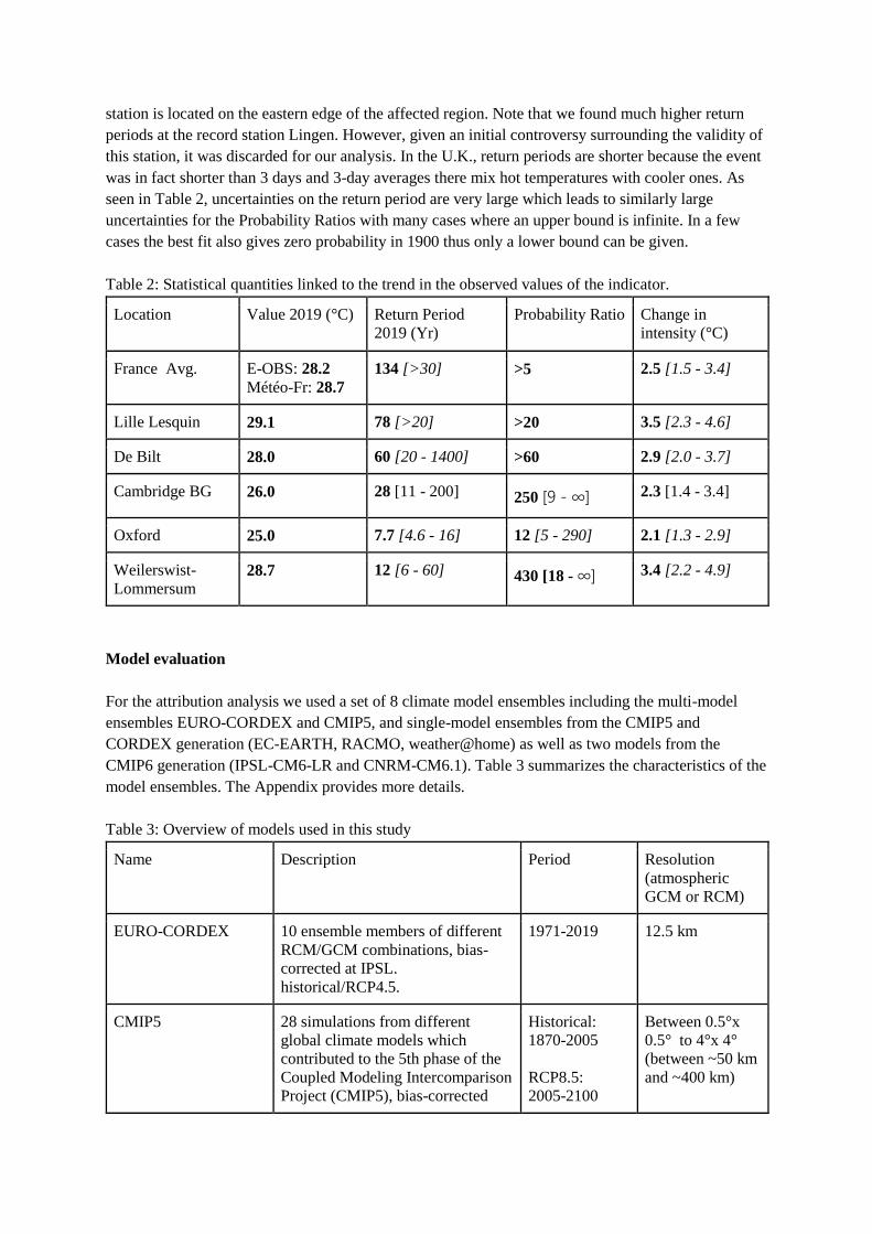
Table 2: Statistical quantities linked to the trend in the observed values of the indicator.

Location Value 2019 (°C) Return Period

2019 (Yr)

Probability Ratio Change in

intensity (°C)

France Avg. E-OBS: 28.2

Météo-Fr: 28.7

134 [>30] >5 2.5 [1.5 - 3.4]

Lille Lesquin 29.1 78 [>20] >20 3.5 [2.3 - 4.6]

De Bilt 28.0 60 [20 - 1400] >60 2.9 [2.0 - 3.7]

Cambridge BG 26.0 28 [11 - 200] 250 [9 - ∞] 2.3 [1.4 - 3.4]

Oxford 25.0 7.7 [4.6 - 16] 12 [5 - 290] 2.1 [1.3 - 2.9]

Weilerswist-

Lommersum 28.7 12 [6 - 60] 430 [18 - ∞] 3.4 [2.2 - 4.9]

Model evaluation

For the attribution analysis we used a set of 8 climate model ensembles including the multi-model

ensembles EURO-CORDEX and CMIP5, and single-model ensembles from the CMIP5 and

CORDEX generation (EC-EARTH, RACMO, weather@home) as well as two models from the

CMIP6 generation (IPSL-CM6-LR and CNRM-CM6.1). Table 3 summarizes the characteristics of the

model ensembles. The Appendix provides more details.

Table 3: Overview of models used in this study

Name Description Period Resolution

(atmospheric

GCM or RCM)

EURO-CORDEX 10 ensemble members of different

RCM/GCM combinations, bias-

corrected at IPSL.

historical/RCP4.5.

1971-2019 12.5 km

CMIP5 28 simulations from different

global climate models which

contributed to the 5th phase of the

Coupled Modeling Intercomparison

Project (CMIP5), bias-corrected

Historical:

1870-2005

RCP8.5:

2005-2100

Between 0.5°x

0.5° to 4°x 4°

(between ~50 km

and ~400 km)

against E-OBS at ETHZ.

weather@home large ensemble of HadRM3P

embedded in HadAM3P with

prescribed SST, counterfactual 11

different SST patterns subtracted

2006-2015 vs

counterfactual

2006-2015

25 km

RACMO 2.2 16 ensemble members downscaling

EC-Earth 2.3 historical/RCP8.5

runs

1950-2019 11 km

HadGEM3-A trend EUCLEIA 15-member ensemble,

SST-forced.

1961-2015 N216 (~60 km)

EC-Earth 2.3 16-member ensemble coupled

GCM, historical/RCP8.5

1861-2019 T159 (~150 km)

IPSL-CM6A-LR 31-member ensemble coupled

GCM, CMIP6 historical (1850-

2014) prolonged until 2029 with

SSP585 forcing except for constant

2014 tropospheric aerosol forcings

1850-2029 144x142 grid

points (~160 km

on average)

CNRM-CM6.1 10-member ensemble coupled

GCM, CMIP6 historical

1850-2014 1.4° at the

equator, with 91

vertical layers

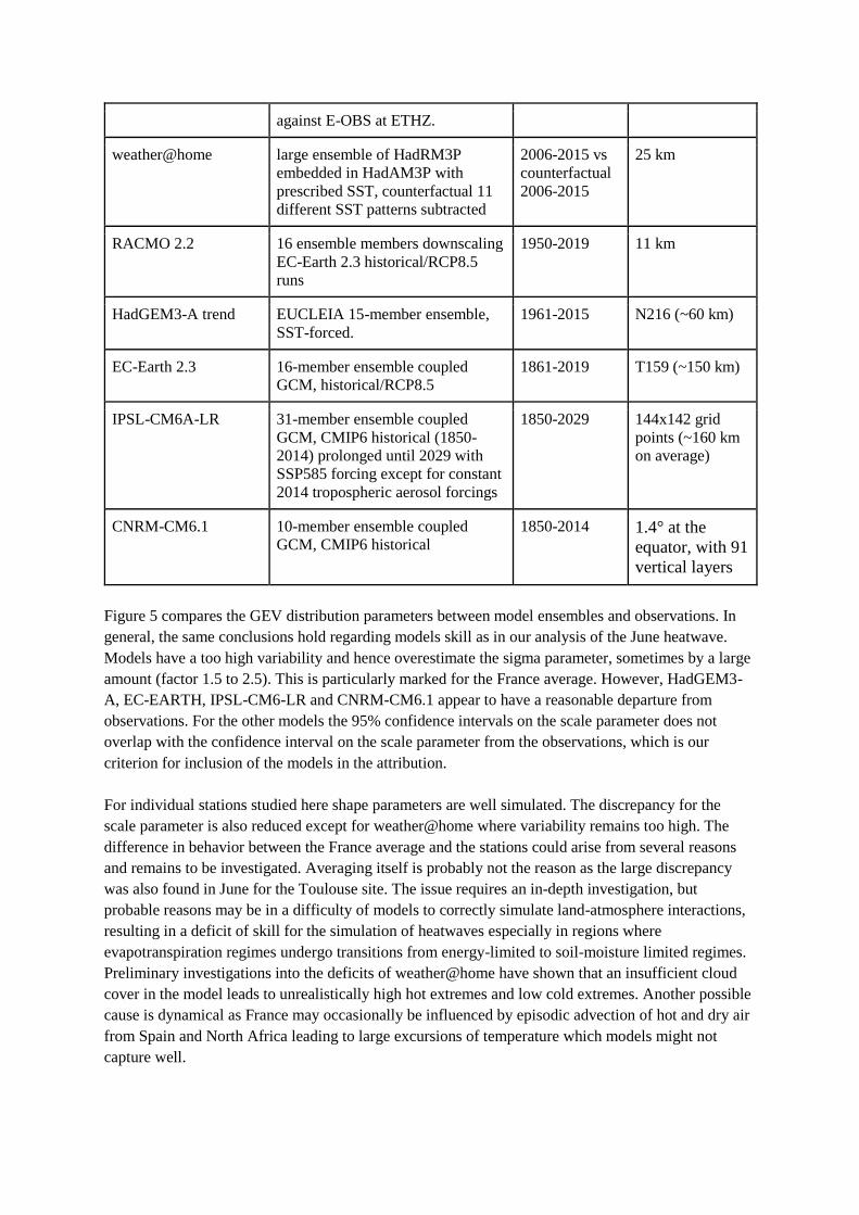
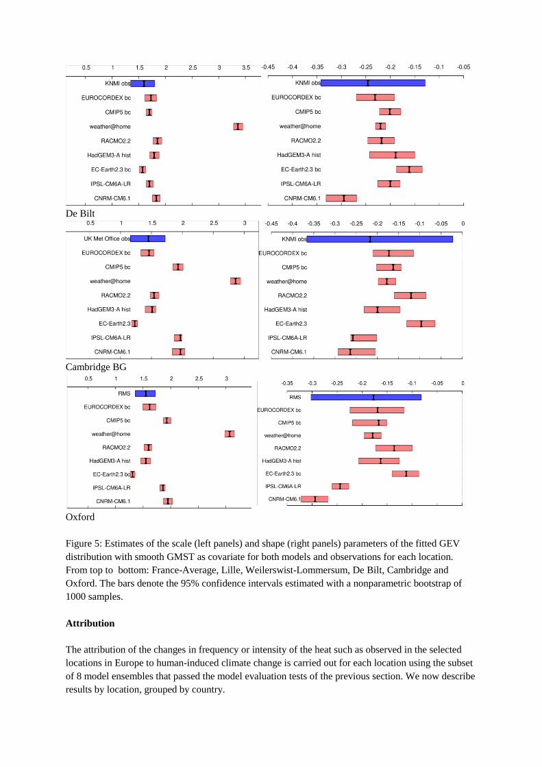
Figure 5 compares the GEV distribution parameters between model ensembles and observations. In

general, the same conclusions hold regarding models skill as in our analysis of the June heatwave.

Models have a too high variability and hence overestimate the sigma parameter, sometimes by a large

amount (factor 1.5 to 2.5). This is particularly marked for the France average. However, HadGEM3-

A, EC-EARTH, IPSL-CM6-LR and CNRM-CM6.1 appear to have a reasonable departure from

observations. For the other models the 95% confidence intervals on the scale parameter does not

overlap with the confidence interval on the scale parameter from the observations, which is our

criterion for inclusion of the models in the attribution.

For individual stations studied here shape parameters are well simulated. The discrepancy for the

scale parameter is also reduced except for weather@home where variability remains too high. The

difference in behavior between the France average and the stations could arise from several reasons

and remains to be investigated. Averaging itself is probably not the reason as the large discrepancy

was also found in June for the Toulouse site. The issue requires an in-depth investigation, but

probable reasons may be in a difficulty of models to correctly simulate land-atmosphere interactions,

resulting in a deficit of skill for the simulation of heatwaves especially in regions where

evapotranspiration regimes undergo transitions from energy-limited to soil-moisture limited regimes.

Preliminary investigations into the deficits of weather@home have shown that an insufficient cloud

cover in the model leads to unrealistically high hot extremes and low cold extremes. Another possible

cause is dynamical as France may occasionally be influenced by episodic advection of hot and dry air

from Spain and North Africa leading to large excursions of temperature which models might not

capture well.

In Lille, weather@home and HadGEM3-A fail the test that the scale parameter is compatible with the

observed range.

At Weilerswist-Lommersum and De Bilt, all models except weather@home pass our model

evaluation criterion of the observed parameter uncertainty range overlapping the modelled ones.

In Cambridge and Oxford, the CMIP5 ensemble, IPSL-CM6A-LR and CNRM-CM6.1 have a too

large scale parameter σ compared to the observations, weather@home much too large. We therefore

do not include these models in the attribution.

France-Average

Lille-Lesquin

Weilerswist-Lommersum

De Bilt

Cambridge BG

Oxford

Figure 5: Estimates of the scale (left panels) and shape (right panels) parameters of the fitted GEV

distribution with smooth GMST as covariate for both models and observations for each location.

From top to bottom: France-Average, Lille, Weilerswist-Lommersum, De Bilt, Cambridge and

Oxford. The bars denote the 95% confidence intervals estimated with a nonparametric bootstrap of

1000 samples.

Attribution

The attribution of the changes in frequency or intensity of the heat such as observed in the selected

locations in Europe to human-induced climate change is carried out for each location using the subset

of 8 model ensembles that passed the model evaluation tests of the previous section. We now describe

results by location, grouped by country.

The attribution is carried out using estimations from a GEV fit with the smoothed GMST covariate as

an indicator of climate change and human activities. The training period for the fit is taken as the

largest possible period between 1900 and 2019 for models and ending in 2018 for the observations in

order not to include the extreme event itself as it would lead to a selection bias. For some model

ensembles the fit was made over a shorter period as the data were not available back to 1900 (such as

for RACMO, EURO-CORDEX and HadGEM3-A). Due to the large ensemble size in the

weather@home simulations no distribution was fitted but a non-parametric comparison of the

observed event in the simulation of the present day climate with the same event in a counterfactual

climate performed.

A synthesis is made based on observations and the model ensembles that passed the evaluation by

weighting the results. The model results are combined with an estimate of model uncertainty such that

the spread in the model results is compatible with the total uncertainty, which is the uncertainty due to

natural variability combined with this model uncertainty (so we fit the model uncertainty to give

χ²/dof = 1). The same model uncertainty is added to the "models" subresult. This subresult is

combined with the observed estimate in two ways: a weighted average denoted by the coloured bar

and an unweighted average denoted by the open bar. As the models have more biases than the spread

indicates we base our conclusions on the latter, which gives more weight to the observations (the

method is described in detail in van Oldenborgh et al, in preparation, a copy of the draft is available

on request).

France

Figure 6 shows attribution results for (i) the average over metropolitan France and (ii) the Lille

station. Detailed numerical results can also be found in the Appendix.

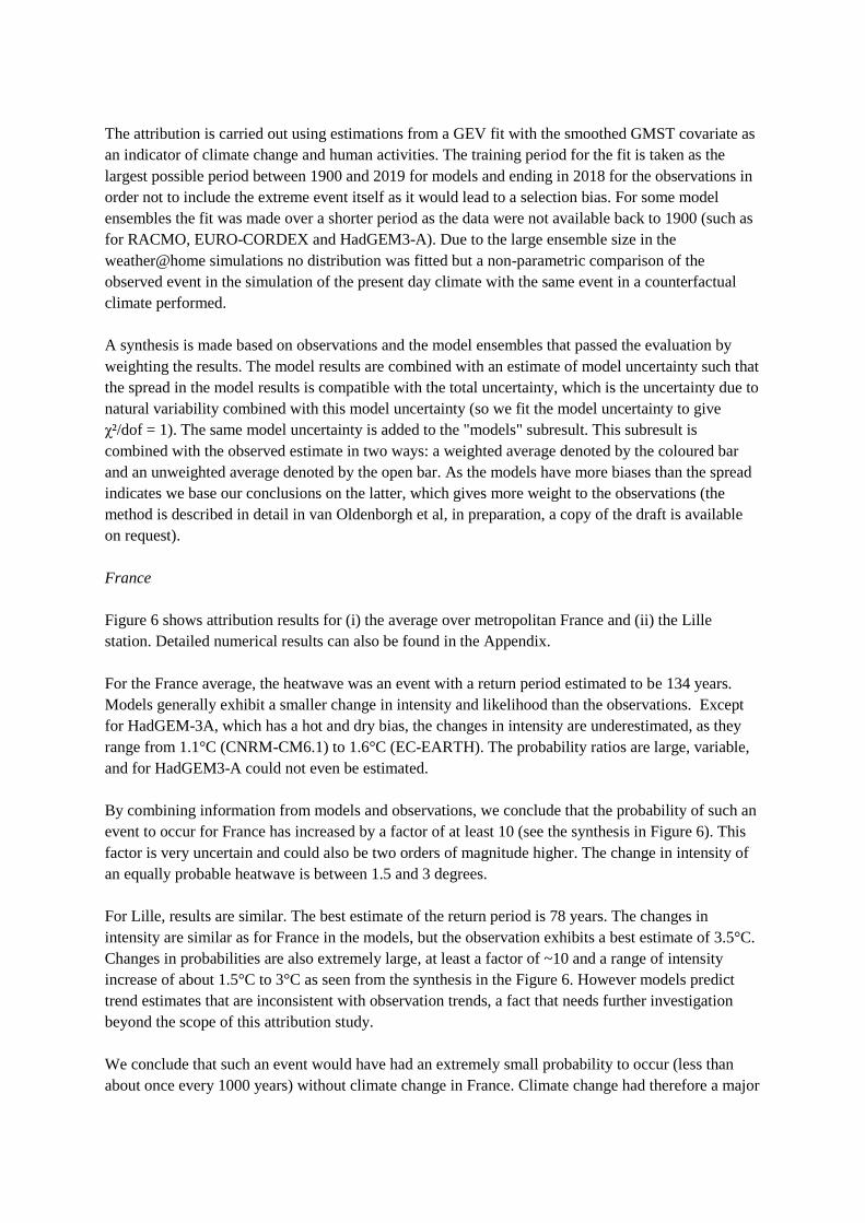
For the France average, the heatwave was an event with a return period estimated to be 134 years.

Models generally exhibit a smaller change in intensity and likelihood than the observations. Except

for HadGEM-3A, which has a hot and dry bias, the changes in intensity are underestimated, as they

range from 1.1°C (CNRM-CM6.1) to 1.6°C (EC-EARTH). The probability ratios are large, variable,

and for HadGEM3-A could not even be estimated.

By combining information from models and observations, we conclude that the probability of such an

event to occur for France has increased by a factor of at least 10 (see the synthesis in Figure 6). This

factor is very uncertain and could also be two orders of magnitude higher. The change in intensity of

an equally probable heatwave is between 1.5 and 3 degrees.

For Lille, results are similar. The best estimate of the return period is 78 years. The changes in

intensity are similar as for France in the models, but the observation exhibits a best estimate of 3.5°C.

Changes in probabilities are also extremely large, at least a factor of ~10 and a range of intensity

increase of about 1.5°C to 3°C as seen from the synthesis in the Figure 6. However models predict

trend estimates that are inconsistent with observation trends, a fact that needs further investigation

beyond the scope of this attribution study.

We conclude that such an event would have had an extremely small probability to occur (less than

about once every 1000 years) without climate change in France. Climate change had therefore a major

influence to explain such temperatures, making them about 100 times more likely (at least a factor of

ten).

Figure 6: Changes in intensity (left panels) and probability ratios (right panels) obtained for all models

and the two stations in France. From top to bottom: France Average, Lille-Lesquin.

Germany

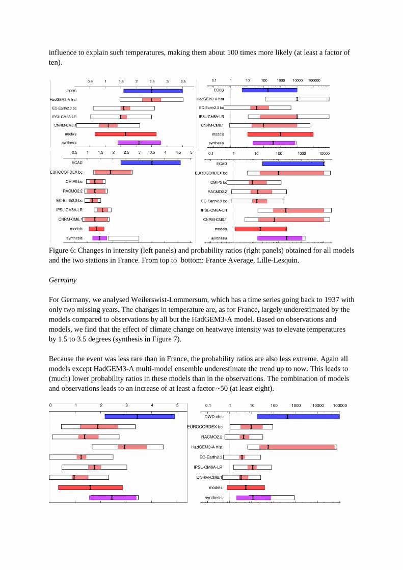
For Germany, we analysed Weilerswist-Lommersum, which has a time series going back to 1937 with

only two missing years. The changes in temperature are, as for France, largely underestimated by the

models compared to observations by all but the HadGEM3-A model. Based on observations and

models, we find that the effect of climate change on heatwave intensity was to elevate temperatures

by 1.5 to 3.5 degrees (synthesis in Figure 7).

Because the event was less rare than in France, the probability ratios are also less extreme. Again all

models except HadGEM3-A multi-model ensemble underestimate the trend up to now. This leads to

(much) lower probability ratios in these models than in the observations. The combination of models

and observations leads to an increase of at least a factor ~50 (at least eight).

Figure 7: Changes in intensity (left panels) and probability ratios (right panels) obtained for all models

and the station of Weilerswist-Lommersum

The Netherlands

The change in temperature of the hottest three days of the year is 2.9±1.0 ºC in the observations and

around 1.5 ºC in all models except HadGEM3-A (which has a dry and warm bias) and EURO-

CORDEX (which has no aerosol changes except for one of the models). The large deviation of

HadGEM3-A from the other models gives rise to a large model spread term (white boxes, which

increases the uncertainty on the model estimate so that it agrees with the observed trend). Without the

HadGEM3-A the models agree well with each other but not with the observations (not shown). The

overall synthesis provides, as for France, an intensity change in the range of 1.5 to 3 degrees.

For the Probability Ratio, we arbitrarily replaced the infinities by 10000 yr and 100000 yr for the

upper bound on the PR of the fit to the observations. As expected the models show (much) lower PRs,

due to the higher variability and lower trends. The models with the lowest trends, EC-Earth and

RACMO, also give the lowest Probability Ratio, around 10. Combining models and observations

gives a best estimate of 300 with a lower bound of 25.

Figure 8: Changes in intensity (left panels) and probability ratios (right panels) obtained for all models

at the station of De Bilt.

U. K.

For U.K. stations, only 4 (Cambridge) and 3 (Oxford) model ensembles were kept in the analysis

based on our selection criteria. As for the other locations, Probability Ratios cover a wide range.

Combining observations and models lead us to conclude that the likelihood of the event has increased

by a factor of ~20 in Cambridge (at least a factor of 3). For Oxford on the other hand, the heatwave

was less extreme in TG3x and the PR numbers are lower.

Interestingly, the change in intensity is better simulated than for other continental locations. Based on

all information we find a rather similar range of temperature trends, from slightly less than 1.5 to ~2.5

degrees. The range is slightly higher for Cambridge than for Oxford.

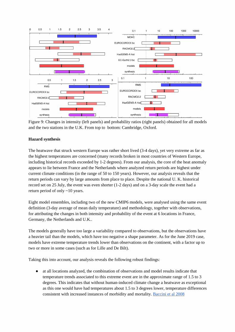
Figure 9: Changes in intensity (left panels) and probability ratios (right panels) obtained for all models

and the two stations in the U.K. From top to bottom: Cambridge, Oxford.

Hazard synthesis

The heatwave that struck western Europe was rather short lived (3-4 days), yet very extreme as far as

the highest temperatures are concerned (many records broken in most countries of Western Europe,

including historical records exceeded by 1-2 degrees). From our analysis, the core of the heat anomaly

appears to lie between France and the Netherlands where analyzed return periods are highest under

current climate conditions (in the range of 50 to 150 years). However, our analysis reveals that the

return periods can vary by large amounts from place to place. Despite the national U. K. historical

record set on 25 July, the event was even shorter (1-2 days) and on a 3-day scale the event had a

return period of only ~10 years.

Eight model ensembles, including two of the new CMIP6 models, were analysed using the same event

definition (3-day average of mean daily temperature) and methodology, together with observations,

for attributing the changes in both intensity and probability of the event at 6 locations in France,

Germany, the Netherlands and U.K..

The models generally have too large a variability compared to observations, but the observations have

a heavier tail than the models, which have too negative a shape parameter. As for the June 2019 case,

models have extreme temperature trends lower than observations on the continent, with a factor up to

two or more in some cases (such as for Lille and De Bilt).

Taking this into account, our analysis reveals the following robust findings:

● at all locations analyzed, the combination of observations and model results indicate that

temperature trends associated to this extreme event are in the approximate range of 1.5 to 3

degrees. This indicates that without human-induced climate change a heatwave as exceptional

as this one would have had temperatures about 1.5 to 3 degrees lower, temperature differences

consistent with increased instances of morbidity and mortality. Baccini et al 2008

● at all locations analyzed, the change in probability of the event is large, and in several cases it

is so large that a reliable estimate cannot be established. In France and the Netherlands, we

find changes of at least a factor 10, meaning that the event would be extremely improbable

without climate change (return period larger than about 1000 years). For the other locations,

changes in probabilities were less impressive but still very large, at least a factor of 2-3 for the

U.K. station, and 8 for the German station.

This analysis, together with the analysis of the June case, triggers several key research questions,

which are:

● what are the physical mechanisms involved in explaining the common model biases in the

extremes (eg. too high variability, too small trends)?

● would one obtain similar results using different statistical methods (only one method has been

applied), and other conditionings?

● are models improving on the simulation of extremes, from the CMIP5 to CMIP6 generation?

● has climate change induced more atmospheric flows favorable to extreme heat, and, vice

versa, for similar flows what are the changes in temperatures?

These yet unsolved questions call for more investigation which could not be carried out in this rapid

attribution study.

Vulnerability and Exposure

Heatwaves are amongst the deadliest natural disasters facing humanity today and their frequency and

intensity is on the rise globally. Consistent with this trend, the July 2019 heatwave across parts of

Europe was made more likely due to climate change, as documented in this study. Combined with

other risk factors such as age, certain non-communicable diseases, socio-economic disadvantages, and

the urban heat island effect, extreme heat impacts become even more acute. (Kovats and Hajat 2008)

The most striking impacts of heatwaves, deaths, are not fully understood until weeks, months or even

years after the initial event. While a few initial deaths due to heat stroke and drowning (from people

attempting to keep cool at beaches and pools) may be reported, these numbers consistently pale in

comparison to deaths resulting from excess mortality. Excess mortality is derived from statistical

analysis comparing deaths during an extreme heat event to the typical projected number of deaths for

the same time period based on historical record. (McGregor et al 2015) Those at highest risk of death

during a heatwave are older people, people with respiratory illnesses, cardiovascular disease and other

pre-existing conditions, homeless, socially isolated, urban residents and others. (McGregor et al 2015)

Deaths among these populations are are not attributable to instances of extreme heat in real time but

become apparent through a public health lens following the event. The 2003 European heatwave was

originally estimated to have 35,000 excess deaths, this number was later estimated to be 70,000

excess deaths in 2008. (Robine et al 2008) The Russian heatwave of 2010 was estimated to have

55,000 excess deaths, due in part to a combination of extreme heat and excess air pollution.

(Shaposhnikov at al 2014) A 2010 heatwave in India was estimated to have caused 1,344 excess

deaths, a 43.1% increase over average, in a 2014 study. (Azhar 2014) This lag time between the

occurrence of the heatwave, and an understanding of excess deaths poses significant barriers to public

action to reduce heat risks. Yet, simple, low cost measures can prevent heat deaths.

Following Europe’s extreme heat event of 2003 many life saving measures have been put in place.

The Netherlands established a ‘National Heatwave Action Plan’, France established the ‘Plane

Canicule’, in Germany a heat wave warning system has been established and The United Kingdom

established ‘The Heatwave Plan for England’. Collectively these plans include many proven good

practices such as: understanding local thresholds where excess heat becomes deadly, establishing

early warning systems, bolstering public communications about heat risks , ensuring people have

access to cool spaces for a few hours a day, such as cooling centers, fountains and green spaces, and

bolstering health systems to be prepared for a surge in demand. (Public Health England 2019, Fouillet

et al 2008, Ebi et al 2004)

However while these strong examples exist, on a whole, Europe is still highly vulnerable to heat

extremes, with approximately 42% of its population over 65 vulnerable to heat risks. (Lancet 2018) In

addition to life saving measures during a heatwave, it is also crucial to catalyze longer-term efforts to

adapt to raising heat risks in Europe. (Bittner et al 2014) This includes increasing urban green spaces,

increasing concentrations of reflective roofs, upgrading building codes to increase passive cooling

strategies, and further bolstering health systems to be prepared for excess case loads. (Singh et al

2019) The City of Paris is one of the cities in Europe leading the way on this effort. Their Paris

Adaptation Strategy includes measures such as: ensuring everyone in the city is a 7-minute walk, or

less, from a green space with drinking water; incorporating durable water cooling systems into the

urban landscape (fountains, reflecting pools, misting systems etc.); planting 20,000 trees; establishing

100 hectares of green roofs; integrating passive cooling measures into new and existing buildings and

updating building codes. (Mairie de Paris 2015) Expanding measures such as these throughout urban

areas across Europe will help to reduce the vulnerability and exposure of Europe’s residents to future

heat extremes.

Acknowledgements:

The study was made possible thanks to a strong international collaboration between several institutes

and organizations in Europe (DWD, ETHZ, IPSL, ITC/Red Cross/Red Crescent, KNMI, Météo-

France, Univ. Oxford, U.K. Met Office), whose teams shared data and methods, and thanks to the

Climate Explorer tool developed by KNMI. It was also supported by the EU ERA4CS “EUPHEME”

research project, grant #690462.

Appendix:

model details:

EURO-CORDEX: we use here an ensemble of 10 GCM-RCM models that were also used in previous

studies for heatwaves, heavy precipitation and storms (see eg. Kew et al., 2019; Luu et al., 2019;

Vautard et al., 2019). These models were bias-adjusted using the CDFt method (Vrac et al., 2016)

using a methodology that was deployed for serving the energy sector within the Copernicus Climate

Change Service (Bartok et al., submitted to Climate Services). It uses historical simulations before

2005 and the RCP4.5 scenario after then.

List of models used for EURO-CORDEX

Global Climate Model Regional Climate Model (downscaling)

1 CNRM-CERFACS-CNRM-CM5 ARPEGE (stretched)

2 CNRM-CERFACS-CNRM-CM5 RCA4

3 ICHEC-EC-ECEARTH RCA4

4 ICHEC-EC-ECEARTH RACMO22E

5 ICHEC-EC-ECEARTH HIRHAM5

6 IPSL-IPSL-CM5A-MR WRF331F

7 MOHC-HadGEM-ES RACMO22E

8 MOHC-HadGEM-ES RCA4

9 MPI-M-MPI-ESM-LR REMO2009

10 MPI-M-MPI-ESM-LR RCA4

CMIP5 global climate model simulations: We use here single runs (r1i1p1) of 28 model simulations

from the 5th phase of the Coupled Modeling Intercomparison Project (CMIP5; Taylor, et.al. 2012) for

historical and future simulations under a high emission scenario (RCP8.5, van Vuuren et al. 2011);

see Table 2) building upon previous analyses with these data (e.g. Vogel et al. 2019). We compute

TG3x between 1870-2100 from daily air temperatures (tas in CMIP5) for each model in the original

resolution and then average over metropolitan France and Toulouse. For the covariate we compute

mean summer temperatures on land over Western European (35°N-72N, 15°W-20°E).

All temperatures from the CMIP5 ensemble simulations are bias corrected to E-OBS (Haylock et al.

2008) temperatures for the reference period 1950-1979 for each model individually. To fit GEVs we

pool the data from the whole CMIP5 ensemble from 1947-2018 which allows a robust estimate.

Table 2. Overview of 28 CMIP5 models used in this study. For each model we use one ensemble

member from the historical period and RCP8.5.

Model name Modeling center

ACCESS1.0 Commonwealth Scientific and Industrial

Research Organization (CSIRO) and Bureau of

Meteorology (BOM), Australia\

ACCESS1.3 Commonwealth Scientific and Industrial

Research Organization (CSIRO) and Bureau of

Meteorology (BOM), Australia\\

BCC-CSM1.1 Beijing Climate Center, China Meteorological

Administration

BCC-CSM1.1M Beijing Climate Center, China Meteorological

Administration

CanESM2 Canadian Centre for Climate Modelling and

Analysis

CCSM4 National Center for Atmospheric Research

CESM1(BGC) Community Earth System Model Contributors

CMCC-CESM Centro Euro-Mediterraneo sui Cambiamenti

Climatic

CMCC-CM Centro Euro-Mediterraneo sui Cambiamenti

Climatici

CMCC-CMs Centro Euro-Mediterraneo sui Cambiamenti

Climatici

CNRM-CM5 Centre National de Recherches Météorologiques

/

Centre Européen de Recherche et Formation

Avancée en Calcul Scientifique\\

CSIRO-Mk3.6.0 Commonwealth Scientific and Industrial

Research Organization in collaboration with

Queensland Climate Change

Centre of Excellence

EC-EARTH European-Earth-System-Model Consortium

GFDL-CM3 NOAA Geophysical Fluid Dynamics

Laboratory

HadGEM2-A0 Met Office Hadley Centre

HadGEM2-CC Met Office Hadley Centre

INM-CM4 Institute for Numerical Mathematics

IPSL-CM5A-LR Institut Pierre-Simon Laplace

IPSL-CM5A-MR Institut Pierre-Simon Laplace

IPSL-CM5B-LR Institut Pierre-Simon Laplace

MIROC-ESM Japan Agency for Marine-Earth Science and

Technology, Atmosphere and Ocean Research

Institute (The University of

Tokyo), and National Institute for

Environmental Studies

MIROC-ESM-CHEM Japan Agency for Marine-Earth Science and

Technology, Atmosphere and Ocean Research

Institute (The University of

Tokyo), and National Institute for

Environmental Studies\\

MIROC5 Atmosphere and Ocean Research Institute (The

University of Tokyo), National Institute for

Environmental Studies, and

Japan Agency for Marine-Earth Science and

Technology \\

MPI-ESM-LR Max-Planck-Institute for Meteorology

MPI-ESM-MR Max-Planck-Institute for Meteorology

MRI-CGCM3 Meteorological Research Institute

MRI-ESM1 Meteorological Research Institute

NorESM1-M Norwegian Climate Centre\

RACMO 2.2: this regional climate model ensemble downscales 16 initial-condition realizations of the

EC-EARTH 2.3 coupled climate model in the CMIP5 RCP8.5 scenario (Lenderink et al., 2014;

Aalbers et al., 2017) on a smaller European domain over 1950-2100.

HadGEM3-A-N216: the atmosphere-only version of the Hadley Centre climate model. For the trend

analysis we use the 15 members run for the EUCLEIA project 1961-2015.

EC-Earth 2.3: a coupled GCM, 16 members using historical/RCP8.5 forcing over 1861-2100

(Hazeleger et al, 2010), each producing a transient climate simulation from 1860 to 2100. The

model resolution is T159 which translates to around 150 km in the European domain. The

underlying scenarios are the historical CMIP5 protocols until the year 2005 and the RCP8.5

scenario (Taylor et al. 2012) from 2006 onwards. Up to about 2030, the historical and

RCP8.5 temperature evolution is very similar.

RACMO is a regional climate model developed at KNMI. An ensemble of sixteen members

was generated to downscale the above-mentioned EC-Earth experiments over the period

1950-2100 at a resolution of about 11km (Lenderink et al., 2014, Aalbers et al., 2017).

The 15 HadGEM3-A atmosphere-only runs from 1960–2015 (Ciavarella et al, 2017) (N216,

about 60km) are evaluated for the separate regions. The model is driven by observed forcings

and sea-surface temperatures (SSTs) (“historical”) and with preindustrial forcings and SSTs

from which the effect of climate change has been subtracted (“historicalNat”). The latter

change has been estimated from the Coupled Model Intercomparison Project phase 5

(CMIP5) ensemble of coupled climate simulations.

Weather@home: Using the distributed computing framework known as weather@home

(Guillod et al., 2017, Massey et al., 2015) we simulate two different large ensembles of June

and July weather, using the Met Office Hadley Centre regional climate model HadRM3P at

25km resolution over Europe embedded in the atmosphere-only global circulation model

HadAM3P. The first set of ensembles represents possible weather under current climate

conditions (prescribed OSTIA sea surface temperatures for 2006-2015). This ensemble is

called the “all forcings” scenario and includes human-caused climate change. The second set

of ensembles represents possible summer weather in a world as it might have been without

anthropogenic climate drivers. This ensemble is called the “natural” or “counterfactual”

scenario with prescribed sea surface temperatures obtained from CMIP5 simulations

(Schaller et al., 2016).

IPSL-CM6A-LR is the latest version of the IPSL climate model which was prepared for

CMIP6 (publications in preparation, Servonnat et al., 2019; Lurton et al., 2019). It couples

the LMDZv6 atmospheric model, the NEMO ocean, sea ice and marine biogeochemistry

model and the ORCHIDEE land surface model. The resolution of the atmospheric model is

144x143 points in longitude and latitude, which corresponds to an average resolution of 160

km, and 79 vertical layers. The resolution of the ocean model is 1°x1° and 75 layers in the

vertical. An ensemble of 31 historical simulations have been run for CMIP6 for the period

1850-2014 and have been prolonged until 2029 with SSP585 radiative forcings (except for

constant 2014 aerosol forcing). LMDZv6 includes a ``New Physics'' package based on a full

rethinking of the parametrizations of turbulence, convection and clouds on which the IPSL-

CM6A-LR climate model is built.

CNRM-CM6.1 is the latest version of the CNRM climate model which was prepared for

CMIP6 (Voldoire et al., 2019). It couples the ARPEGE model for the atmosphere, NEMO for

the ocean, ISAB-CTRIP for land surface, GELATO for sea ice. The atmospheric horizontal

resolution is about 1.4° at the equator, with 91 vertical layers. The atmospheric and land

surface models have been subject to major improvements since the CMIP5 exercice, and the

model exhibits a higher equilibrium climate sensitivity (4.9°C). Simulations performed in the

framework of the CMIP6 exercice included 10 historical runs, extending from 1850 to 2014,

and SSP585 scenarios, which were used in this analysis.

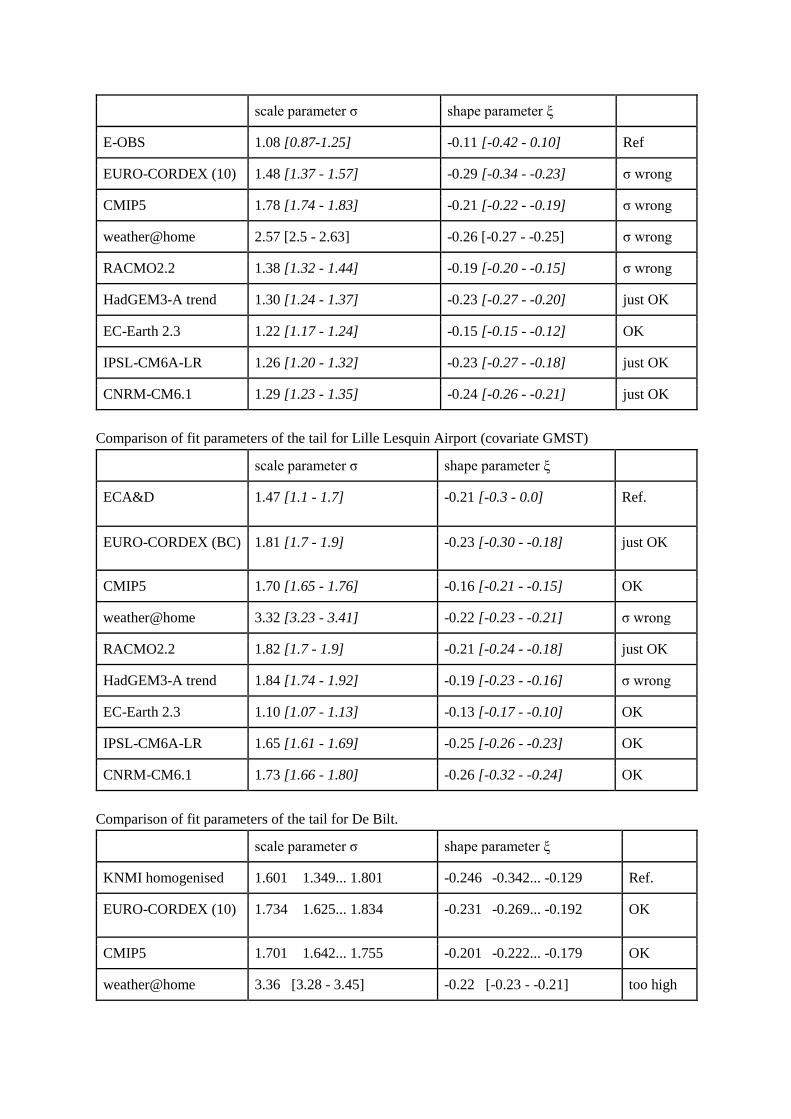
Model evaluation details

Comparison of fit parameters of the tail for France average (covariate GMST)

scale parameter σ shape parameter ξ

E-OBS 1.08 [0.87-1.25] -0.11 [-0.42 - 0.10] Ref

EURO-CORDEX (10) 1.48 [1.37 - 1.57] -0.29 [-0.34 - -0.23] σ wrong

CMIP5 1.78 [1.74 - 1.83] -0.21 [-0.22 - -0.19] σ wrong

weather@home 2.57 [2.5 - 2.63] -0.26 [-0.27 - -0.25] σ wrong

RACMO2.2 1.38 [1.32 - 1.44] -0.19 [-0.20 - -0.15] σ wrong

HadGEM3-A trend 1.30 [1.24 - 1.37] -0.23 [-0.27 - -0.20] just OK

EC-Earth 2.3 1.22 [1.17 - 1.24] -0.15 [-0.15 - -0.12] OK

IPSL-CM6A-LR 1.26 [1.20 - 1.32] -0.23 [-0.27 - -0.18] just OK

CNRM-CM6.1 1.29 [1.23 - 1.35] -0.24 [-0.26 - -0.21] just OK

Comparison of fit parameters of the tail for Lille Lesquin Airport (covariate GMST)

scale parameter σ shape parameter ξ

ECA&D 1.47 [1.1 - 1.7] -0.21 [-0.3 - 0.0] Ref.

EURO-CORDEX (BC) 1.81 [1.7 - 1.9] -0.23 [-0.30 - -0.18] just OK

CMIP5 1.70 [1.65 - 1.76] -0.16 [-0.21 - -0.15] OK

weather@home 3.32 [3.23 - 3.41] -0.22 [-0.23 - -0.21] σ wrong

RACMO2.2 1.82 [1.7 - 1.9] -0.21 [-0.24 - -0.18] just OK

HadGEM3-A trend 1.84 [1.74 - 1.92] -0.19 [-0.23 - -0.16] σ wrong

EC-Earth 2.3 1.10 [1.07 - 1.13] -0.13 [-0.17 - -0.10] OK

IPSL-CM6A-LR 1.65 [1.61 - 1.69] -0.25 [-0.26 - -0.23] OK

CNRM-CM6.1 1.73 [1.66 - 1.80] -0.26 [-0.32 - -0.24] OK

Comparison of fit parameters of the tail for De Bilt.

scale parameter σ shape parameter ξ

KNMI homogenised 1.601 1.349... 1.801 -0.246 -0.342... -0.129 Ref.

EURO-CORDEX (10) 1.734 1.625... 1.834 -0.231 -0.269... -0.192 OK

CMIP5 1.701 1.642... 1.755 -0.201 -0.222... -0.179 OK

weather@home 3.36 [3.28 - 3.45] -0.22 [-0.23 - -0.21] too high

RACMO2.2 1.851 1.770... 1.934 -0.218 -0.246... -0.192 OK

HadGEM3-A trend 1.793 1.706... 1.880 -0.189 -0.242... -0.150 OK

EC-Earth 2.3 bc 1.574 1.511... 1.629 -0.161 -0.187... -0.135 bc

IPSL-CM6A-LR 1.704 1.645... 1.768 -0.200 -0.225... -0.180 OK

CNRM-CM6.1 1.830 1.757... 1.901 -0.295 -0.331... -0.269 OK

Comparison of fit parameters of the tail for Weilerswist-Lommersum.

scale parameter σ shape parameter ξ

DWD 1.594 1.320... 1.816 -0.199 -0.338... -0.101 Ref

EURO-CORDEX (10) 1.791 1.648... 1.903 -0.221 -0.253... -0.160 OK

CMIP5* 1.95 [1.9 - 2.0] -0.19 [-0.21 - -0.18] σ wrong

weather@home 3.53362 [3.44117, 3.62855] -0.237846 [-0.251033, -

0.224659]

σ wrong

RACMO2.2 1.707 1.615... 1.799 -0.196 -0.220... -0.144 OK

HadGEM3-A trend 1.663 1.585... 1.798 -0.194 -0.265... -0.145 OK

EC-Earth 2.3 1.375 1.341... 1.455 -0.131 -0.168... -0.107 OK

IPSL-CM6A-LR* 1.705 1.664... 1.747 -0.241 -0.257... -0.225 OK

CNRM-CM6.1* 1.810 1.738... 1.879 -0.280 -0.306... -0.255 OK

*at the location of Lingen, 200 km to the north.

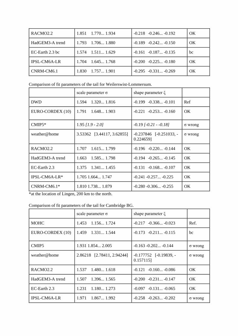
Comparison of fit parameters of the tail for Cambridge BG.

scale parameter σ shape parameter ξ

MOHC 1.453 1.156... 1.724 -0.217 -0.366... -0.023 Ref.

EURO-CORDEX (10) 1.459 1.331... 1.544 -0.173 -0.211... -0.115 bc

CMIP5 1.931 1.854... 2.005 -0.163 -0.202... -0.144 σ wrong

weather@home 2.86218 [2.78411, 2.94244] -0.177752 [-0.19839, -

0.157115]

σ wrong

RACMO2.2 1.537 1.480... 1.618 -0.121 -0.160... -0.086 OK

HadGEM3-A trend 1.507 1.396... 1.565 -0.200 -0.231... -0.147 OK

EC-Earth 2.3 1.231 1.180... 1.273 -0.097 -0.131... -0.065 OK

IPSL-CM6A-LR 1.971 1.867... 1.992 -0.258 -0.263... -0.202 σ wrong

CNRM-CM6.1 1.967 1.842... 2.036 -0.264 -0.293... -0.205 σ wrong

Comparison of fit parameters of the tail for Oxford.

scale parameter σ shape parameter ξ

RMS 1.55 1.359 1.716 -0.177 -0.302 -0.082 Ref.

EURO-CORDEX (10) 1.616 1.499 1.728 -0.169 -0.224 -0.116 bc

CMIP5 1.934 1.872 1.997 -0.167 -0.219 -0.151 bc

weather@home 3.06572 2.98365 3.15004 -0.179126 -0.195901 -

0.162352

RACMO2.2 1.595 1.524 1.657 -0.136 -0.173 -0.100

HadGEM3-A trend 1.548 1.464 1.631 -0.163 -0.207 -0.126

EC-Earth 2.3 1.310 1.267 1.348 -0.112 -0.140 -0.087

IPSL-CM6A-LR 1.859 1.811 1.899 -0.244 -0.260 -0.227

CNRM-CM6.1 1.953 1.869 2.028 -0.294 -0.322 -0.268

Attribution details

Changes for Metropolitan France average. Grey indicates models that did not pass the model

evaluation test, notably because the variability is incompatible with the observations (too high).

ref yrs Return

Value (°C)

RP=134yr

Probability Ratio Change in

temperature (°C)

E-OBS 1950-2018 28.2 179 [>5] 2.5 [1.6-3.5]

EURO-CORDEX 1971-2019 27.9 > 400 1.9 [1.2-2.6]

CMIP5 1900-2019 26.1 11 [5-21] 1.2 [0.9-1.4]

weather@home counterfactual

2006-2015

7.33 (3.24 - 23.21) 1.88

RACMO2.2 1950-2019 25.2 75 [>18] 1.6 [1.3-1.9]

HadGEM3-A 1960-2015 28.0 infinite 2.5 [2.2-2.8]

EC-Earth2.3 1900-2019 25.0 37 [16-200] 1.6 [1.5-1.8]

IPSL-CM6A-LR 1900-2019 28.6 28000 [>60] 1.5 [1.5-1.7]

CNRM-CM6.1 1900-2014 28.1 98 [>19] 1.1 [0.8-1.4]

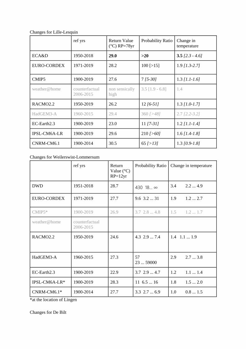
Changes for Lille-Lesquin

ref yrs Return Value

(°C) RP=78yr

Probability Ratio Change in

temperature

ECA&D 1950-2018 29.0 >20 3.5 [2.3 - 4.6]

EURO-CORDEX 1971-2019 28.2 100 [>15] 1.9 [1.3-2.7]

CMIP5 1900-2019 27.6 7 [5-30] 1.3 [1.1-1.6]

weather@home counterfactual

2006-2015

non sensically

high

3.5 [1.9 - 6.8] 1.4

RACMO2.2 1950-2019 26.2 12 [6-51] 1.3 [1.0-1.7]

HadGEM3-A 1960-2015 29.4 360 [>48] 2.7 [2.2-3.2]

EC-Earth2.3 1900-2019 23.0 11 [7-31] 1.2 [1.1-1.4]

IPSL-CM6A-LR 1900-2019 29.6 210 [>60] 1.6 [1.4-1.8]

CNRM-CM6.1 1900-2014 30.5 65 [>13] 1.3 [0.9-1.8]

Changes for Weilerswist-Lommersum

ref yrs Return

Value (°C)

RP=12yr

Probability Ratio Change in temperature

DWD 1951-2018 28.7 430 18... ∞ 3.4 2.2 ... 4.9

EURO-CORDEX 1971-2019 27.7 9.6 3.2 ... 31 1.9 1.2 ... 2.7

CMIP5* 1900-2019 26.9 3.7 2.8 ... 4.8 1.5 1.2 ... 1.7

weather@home counterfactual

2006-2015

RACMO2.2 1950-2019 24.6 4.3 2.9 ... 7.4 1.4 1.1 ... 1.9

HadGEM3-A 1960-2015 27.3 57

23 ... 59000

2.9 2.7 ... 3.8

EC-Earth2.3 1900-2019 22.9 3.7 2.9 ... 4.7 1.2 1.1 ... 1.4

IPSL-CM6A-LR* 1900-2019 28.3 11 6.5 ... 16 1.8 1.5 ... 2.0

CNRM-CM6.1* 1900-2014 27.7 3.3 2.7 ... 6.9 1.0 0.8 ... 1.5

*at the location of Lingen

Changes for De Bilt

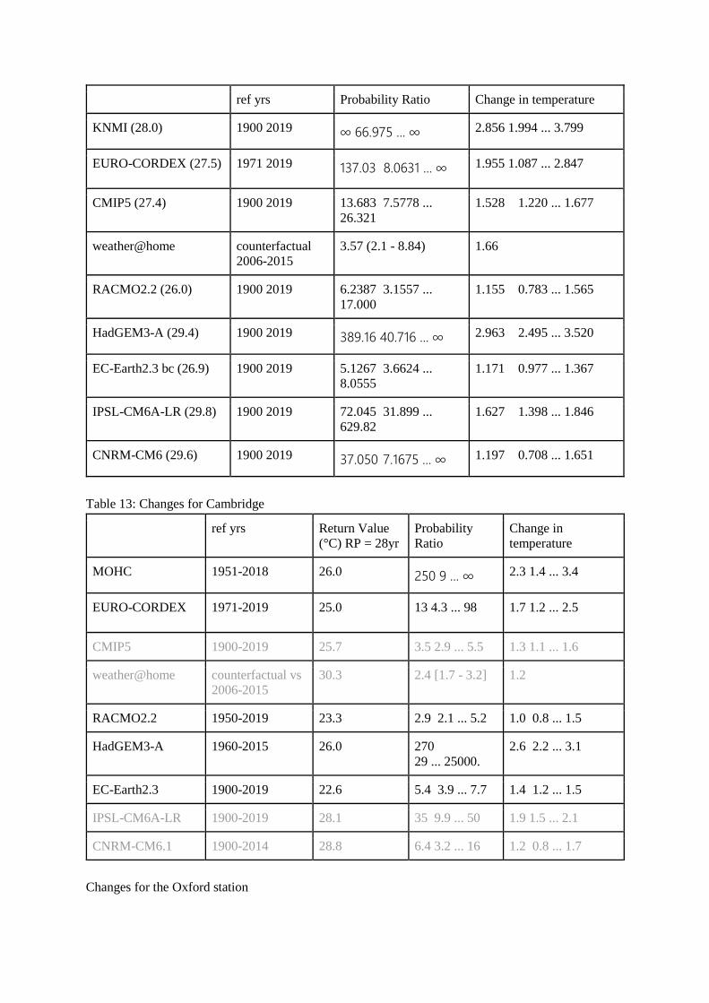
ref yrs Probability Ratio Change in temperature

KNMI (28.0) 1900 2019 ∞ 66.975 ... ∞ 2.856 1.994 ... 3.799

EURO-CORDEX (27.5) 1971 2019 137.03 8.0631 ... ∞ 1.955 1.087 ... 2.847

CMIP5 (27.4) 1900 2019 13.683 7.5778 ...

26.321

1.528 1.220 ... 1.677

weather@home counterfactual

2006-2015

3.57 (2.1 - 8.84) 1.66

RACMO2.2 (26.0) 1900 2019 6.2387 3.1557 ...

17.000

1.155 0.783 ... 1.565

HadGEM3-A (29.4) 1900 2019 389.16 40.716 ... ∞ 2.963 2.495 ... 3.520

EC-Earth2.3 bc (26.9) 1900 2019 5.1267 3.6624 ...

8.0555

1.171 0.977 ... 1.367

IPSL-CM6A-LR (29.8) 1900 2019 72.045 31.899 ...

629.82

1.627 1.398 ... 1.846

CNRM-CM6 (29.6) 1900 2019 37.050 7.1675 ... ∞ 1.197 0.708 ... 1.651

Table 13: Changes for Cambridge

ref yrs Return Value

(°C) RP = 28yr

Probability

Ratio

Change in

temperature

MOHC 1951-2018 26.0 250 9 ... ∞ 2.3 1.4 ... 3.4

EURO-CORDEX 1971-2019 25.0 13 4.3 ... 98 1.7 1.2 ... 2.5

CMIP5 1900-2019 25.7 3.5 2.9 ... 5.5 1.3 1.1 ... 1.6

weather@home counterfactual vs

2006-2015

30.3 2.4 [1.7 - 3.2] 1.2

RACMO2.2 1950-2019 23.3 2.9 2.1 ... 5.2 1.0 0.8 ... 1.5

HadGEM3-A 1960-2015 26.0 270

29 ... 25000.

2.6 2.2 ... 3.1

EC-Earth2.3 1900-2019 22.6 5.4 3.9 ... 7.7 1.4 1.2 ... 1.5

IPSL-CM6A-LR 1900-2019 28.1 35 9.9 ... 50 1.9 1.5 ... 2.1

CNRM-CM6.1 1900-2014 28.8 6.4 3.2 ... 16 1.2 0.8 ... 1.7

Changes for the Oxford station

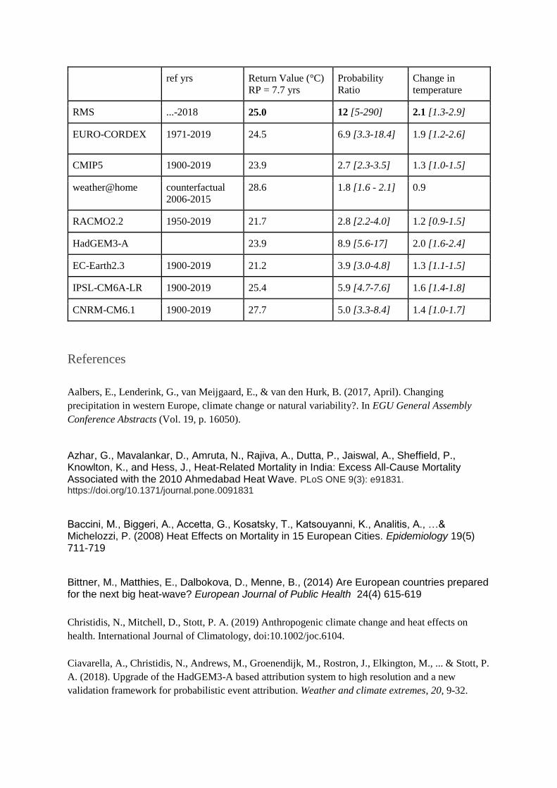
ref yrs Return Value (°C)

RP = 7.7 yrs

Probability

Ratio

Change in

temperature

RMS ...-2018 25.0 12 [5-290] 2.1 [1.3-2.9]

EURO-CORDEX 1971-2019 24.5 6.9 [3.3-18.4] 1.9 [1.2-2.6]

CMIP5 1900-2019 23.9 2.7 [2.3-3.5] 1.3 [1.0-1.5]

weather@home counterfactual

2006-2015

28.6 1.8 [1.6 - 2.1] 0.9

RACMO2.2 1950-2019 21.7 2.8 [2.2-4.0] 1.2 [0.9-1.5]

HadGEM3-A 23.9 8.9 [5.6-17] 2.0 [1.6-2.4]

EC-Earth2.3 1900-2019 21.2 3.9 [3.0-4.8] 1.3 [1.1-1.5]

IPSL-CM6A-LR 1900-2019 25.4 5.9 [4.7-7.6] 1.6 [1.4-1.8]

CNRM-CM6.1 1900-2019 27.7 5.0 [3.3-8.4] 1.4 [1.0-1.7]

References

Aalbers, E., Lenderink, G., van Meijgaard, E., & van den Hurk, B. (2017, April). Changing

precipitation in western Europe, climate change or natural variability?. In EGU General Assembly

Conference Abstracts (Vol. 19, p. 16050).

Azhar, G., Mavalankar, D., Amruta, N., Rajiva, A., Dutta, P., Jaiswal, A., Sheffield, P., Knowlton, K., and Hess, J., Heat-Related Mortality in India: Excess All-Cause Mortality Associated with the 2010 Ahmedabad Heat Wave. PLoS ONE 9(3): e91831. https://doi.org/10.1371/journal.pone.0091831

Baccini, M., Biggeri, A., Accetta, G., Kosatsky, T., Katsouyanni, K., Analitis, A., …& Michelozzi, P. (2008) Heat Effects on Mortality in 15 European Cities. Epidemiology 19(5) 711-719

Bittner, M., Matthies, E., Dalbokova, D., Menne, B., (2014) Are European countries prepared for the next big heat-wave? European Journal of Public Health 24(4) 615-619

Christidis, N., Mitchell, D., Stott, P. A. (2019) Anthropogenic climate change and heat effects on

health. International Journal of Climatology, doi:10.1002/joc.6104.

Ciavarella, A., Christidis, N., Andrews, M., Groenendijk, M., Rostron, J., Elkington, M., ... & Stott, P.

A. (2018). Upgrade of the HadGEM3-A based attribution system to high resolution and a new

validation framework for probabilistic event attribution. Weather and climate extremes, 20, 9-32.

Ebi, K. L., Teisberg, T. J., Kalkstein, L. S., Robinson, L., & Weiher, R. F. (2004). Heat Watch/

Warning Systems Save Lives: Estimated Costs and Benefits for Philadelphia 1995–98. Bulletin of the

American Meteorological Society, 85(8), 1067-1074. doi:10.1175/bams-85-8-1067

Fouillet, A., Rey, G., Wagner, V., Laaidi, K., Empereur-Bissonnet, P., Le Tertre, A., ... & Jougla, E.

(2008). Has the impact of heat waves on mortality changed in France since the European heat wave of

summer 2003? A study of the 2006 heat wave. International journal of epidemiology, 37(2), 309-317.

Guillod, B., Jones, R. G., Bowery, A., Haustein, K., Massey, N. R., Mitchell, D. M., ... & Wilson, S.

(2017). weather@ home 2: validation of an improved global–regional climate modelling system.

Geoscientific Model Development, 10(5), 1849-1872.

Haylock, M. R., Hofstra, N., Klein Tank, A. M. G., Klok, E. J., Jones, P. D., and New, M. (2008) A

European daily high-resolution gridded data set of surface temperature and precipitation for 1950–

2006, J. Geophys. Res., 113, D20119, https://doi.org/10.1029/2008JD010201.

Hazeleger, W., Severijns, C., Semmler, T., Ştefănescu, S., Yang, S., Wang, X., ... & Bougeault, P.

(2010). EC-Earth: a seamless earth-system prediction approach in action. Bulletin of the American

Meteorological Society, 91(10), 1357-1364.

Kew, S. et al, (2019) The exceptional summer heatwave in Southern {Europe} 2017. Bull. Amer.

Met. Soc., 100, S2-S5. doi:10.1175/BAMS-D-18-0109.1

Kovats, S. and Hajat, S. (2008) Heat Stress and Public Health: A Critical Review. Annual Review

Public Health 29, 41-55 doi: 10.1146/annurev.publhealth.29.020907.090843

Lenderink, G., Van den Hurk, B. J. J. M., Tank, A. K., Van Oldenborgh, G. J., Van Meijgaard, E., De

Vries, H., & Beersma, J. J. (2014). Preparing local climate change scenarios for the Netherlands using

resampling of climate model output. Environmental Research Letters, 9(11), 115008.

Luu, L., R. Vautard, P. Yiou, G. J. van Oldenborgh, and G. Lenderink, 2018, Attribution of

extreme rainfall events in the South of France using EURO-CORDEX simulations. Geophys.

Res. Lett., doi :10.1029/2018GL077807.

Mairie de Paris (2015) Adaptation Strategy: Paris Climate & Energy Action Plan Available at:

https://api-site.paris.fr/images/76271

Massey, N., Jones, R., Otto, F. E. L., Aina, T., Wilson, S., Murphy, J. M., ... & Allen, M. R.

(2015). weather@ home—development and validation of a very large ensemble modelling

system for probabilistic event attribution. Quarterly Journal of the Royal Meteorological

Society, 141(690), 1528-1545.

McGregor, G. R., Bessemoulin, R., Ebi, K., & Menne, B. (Eds.). (2015). Heatwaves and

health: Guidance on warning-system development (Vol. 1142). Geneva, Switzerland, World

Meteorological Organization and World Health Organisation. Retrieved from: http://bit.

ly/2NbDx4S

Murray, V., & Ebi, K. L. (2012). IPCC special report on managing the risks of extreme

events and disasters to advance climate change adaptation (SREX).

Otto, F.E.L., van der Wiel, K., van Oldenborgh, G.J., Philip, S., Kew, S.F., Uhe, P. and

Cullen, H. (2017) Climate change increases the probability of heavy rains in Northern

England/Southern Scotland like those of storm Desmond - a real-time event attribution

revisited. Environmental Research Letters.

Philip, S., Kew, S.F., van Oldenborgh, G.J., Aalbers, E., Vautard, R., Otto, F., Haustein, K.,

Habets, F. and Singh, R. (2018) Validation of a Rapid Attribution of the May/June 2016

Flood-Inducing, Precipitation in France to Climate Change. Journal of Hydrometeorology, 19:

1881-1898.

Public Health England (2019). Heatwave plan for England. London, UK, Crown copyright

http://bit.ly/31XMamQ

Robine, J., Cheung, S., Le Roy, S., Van Oyen, H. Griffiths, C., Michel, JP., Hermann, FR., (2008)

Death toll exceeds 70,000 in Europe during the summer of 2003. Comptes Rendus Biologies 331(2)

171-8 doi: 10.1016/j.crvi.2007.12.001

Schaller, N., A. L. Kay, R. Lamb, N. R. Massey, G.-J. van Oldenborgh, F. E. L. Otto, S. N. Sparrow, R.

Vautard, P. Yiou, A. Bowery, S. M. Crooks, C. Huntingford, W. Ingram, R. Jones, T. Legg, J. Miller, J.

Skeggs, D. Wallom, S. Wilson & M. R. Allen, 2015, Human influence on climate in the 2014 Southern

England winter floods and their impacts. Nature climate change, doi:10.1038/nclimate2927.

Seneviratne S.I., T. Corti, E.L. Davin, M. Hirschi, E.B. Jaeger, I. Lehner, B. Orlowsky and

A.J. Teuling (2010) Investigating soil moisture-climate interactions in a

changing climate: A review. Earth Sci. Rev., 99,125–161.

Singh, R., Arrighi, J., Jjemba, E., Strachan, K., Spires, M., Kadihasanoglu, A., (2019)

Heatwave Guide for Cities. Red Cross Red Crescent Climate Centre.

Stott PA, Stone DA, Allen MR. (2004) Human contribution to the European heatwave of

2003, Nature, 432, 7017, 610-614, DOI:10.1038/nature03089.

Taylor, K. E., R. J. Stouffer, and G. A. Meehl (2012) An overview of CMIP5 and the

experiment design, Bull. Am. Meteorol. Soc., 93(4), 485–498.

van Vuuren, D.P., Edmonds, J., Kainuma, M. et al. Climatic Change (2011) 109, 5.

https://doi.org/10.1007/s10584-011-0148-z

Vautard, R., van Oldenborgh, G.-J., Otto, F. E. L., Yiou, P., de Vries, H., van Meijgaard, E., Stepek,

A., Soubeyroux, J.-M., Philip, S., Kew, S. F., Costella, C., Singh, R., and C. Tebaldi, 2019: Human

influence on European wind storms such as those of January 2018. Earth System Dynamics, 10, 271-

286.

Vogel M.M., J. Zscheischler, R. Wartenburger, D. Dee, and S.I. Seneviratne (2019,

accepted). Concurrent 2018 hot extremes across Northern Hemisphere due to human-

induced climate change. Earth’s Future 7, https://doi.org/10.1029/2019EF001189.

Vrac, M., Noël, T. and R. Vautard, 2016: Bias correction of precipitation through Singularity

Stochastic Removal: Because occurrences matter, J. Geophys. Res., 121(10), 5237-5258.