Draft version June 12, 2018Preprint typeset using LATEX style emulateapj v. 05/12/14

METHANE, CARBON MONOXIDE, AND AMMONIA IN BROWN DWARFS AND SELF-LUMINOUS GIANTPLANETS

Kevin J. ZahnleNASA Ames Research Center, MS-245-3, Moffett Field, CA 94035; Kevin.J.Zahnle@NASA.gov

Mark S. MarleyNASA Ames Research Center, MS-245-3, Moffett Field, CA 94035; Mark.S.Marley@NASA.gov

Draft version June 12, 2018

ABSTRACT

We address disequilibrum abundances of some simple molecules in the atmospheres of solar compo-sition brown dwarfs and self-luminous extrasolar giant planets using a kinetics-based 1D atmosphericchemistry model. Our approach is to use the full kinetics model to survey the parameter space witheffective temperatures between 500 K and 1100 K. In all of these worlds equilibrium chemistry favorsCH4 over CO in the parts of the atmosphere that can be seen from Earth, but in most disequilibriumfavors CO. The small surface gravity of a planet strongly discriminates against CH4 when compared toan otherwise comparable brown dwarf. If vertical mixing is like Jupiter’s, the transition from methaneto CO occurs at 500 K in a planet. Sluggish vertical mixing can raise this to 600 K; but clouds ormore vigorous vertical mixing could lower this to 400 K. The comparable thresholds in brown dwarfsare 1100 ± 100 K. Ammonia is also sensitive to gravity, but unlike CH4/CO, the NH3/N2 ratio isinsensitive to mixing, which makes NH3 a potential proxy for gravity. HCN may become interestingin high gravity brown dwarfs with very strong vertical mixing. Detailed analysis of the CO-CH4

reaction network reveals that the bottleneck to CO hydrogenation goes through methanol, in partialagreement with previous work. Simple, easy to use quenching relations are derived by fitting to thecomplete chemistry of the full ensemble of models. These relations are valid for determining CO,CH4, NH3, HCN, and CO2 abundances in the range of self-luminous worlds we have studied but maynot apply if atmospheres are strongly heated at high altitudes by processes not considered here (e.g.,wave breaking).

1. INTRODUCTION

Disequilibrium chemistry has been known in Jupiter’satmosphere for several decades (Prinn and Barshay 1977;Bezard et al. 2002) and has been expected and sus-pected in brown dwarf atmospheres from the time of theirdiscovery (Fegley and Lodders 1996; Noll et al. 1997;Saumon et al. 2000). The most famous disequilibriumis an overabundance of CO relative to CH4. This oc-curs in Jupiter and brown dwarfs when CO is dredgedup from deep, hot layers of the atmosphere more quicklythan chemical reactions with ambient hydrogen can con-vert it to CH4. It is to be expected that similar pro-cesses take place in young, self-luminous extrasolar giantplanets. But the apparent paucity of methane in theatmospheres of planets with effective temperatures com-parable to those of methane-rich T-type brown dwarfswas underpredicted and has been met with surprise.

Among field brown dwarfs methane appears—bydefinition—at the L to T-type transition where theirnear-infrared colors turn to the blue at effective tempera-tures near 1200 K (Kirkpatrick 2005). The first directlyimaged planets, however, were found to have effectivetemperatures below 1200 K and yet their near-infraredspectra were devoid of signs of methane in K band (e.g.,Barman et al. 2011a). The best example is HR8799c:despite an effective temperature near 1100 K, in bothlow and high resolution spectra—particularly the highresolution spectrum taken by Konopacky et al. (2013)—methane has gone missing.

Surface gravity is the defining difference between ex-trasolar giant planets and brown dwarfs, and to dateis the only proven difference, although there are greathopes for metallicity. Field brown dwarfs (hereafter BDs)have high surface gravities (g of order 105 cm/s2) andtherefore very compressed scale heights. Extrasolar gi-ant planets (EGPs) have modest surface gravities (g oforder 103 cm/s2) and extended scale heights (e.g., Bur-rows et al. 1997; Saumon & Marley 2008)1. A BD and aself-luminous EGP of the same composition and the sameeffective temperature will have similar optical depths as afunction of temperature, at least in the absence of clouds;i.e., the function T (τ) is roughly the same. However, be-cause p ∝ τg, the BD has a much higher pressure ata given optical depth than does the EGP, and a BD ismuch cooler than the EGP at a given pressure. Becauselower temperatures and higher pressure favor CH4 in itsstruggle with CO, it has been pointed out that CH4 willbe more easily seen and CO less easily seen at lower grav-ity in BDs (Hubeny and Burrows 2007). Hence Barmanet al. (2011a) suggested that the even lower gravity ofHR8799b might be why no methane is seen in it. Weagree. We will verify that the dependence on g is strongand leads to qualitatively different outcomes for BDs andself-luminous EGPs, a result implicit in previous workbut far from fully appreciated.

1 We do not intend to wade into the nomenclature battles here.For our purposes companion objects below ∼ 13 MJ are planets.

arX

iv:1

408.

6283

v2 [

astr

o-ph

.EP]

10

Oct

201

4

2 Zahnle & Marley

Previous studies of carbon speciation in BDs and EGPshave mostly focused on a few particular objects (Saumonet al. 2006; Geballe et al. 2009; Barman et al. 2011a,b;Moses et al. 2011; Line et al. 2011), or on hot highlyirradiated EGPs (Moses et al. 2011; Visscher 2012), orused one of several quench approximations culled fromthe literature (Fegley and Lodders 1996; Saumon et al.2000; Lodders and Fegley 2002; Hubeny and Burrows2007), or various combinations of the above (Cooper andShowman 2006; Visscher and Moses 2011; Moses et al.2013a,b). The basic idea is that CH4 and CO will oftenbe seen in disequilibrium because the chemical reactionsthat would enforce equilibrium don’t have time enoughto take place while the gas is cool (Prinn and Barshay1977). The disequilibrium composition that results isdescribed as “frozen-in” or “quenched.”

Quenching has been widely used to quantify discus-sions of CO-CH4 and N2-NH3 disequilibria in a widerange of astrophysical problems, dating at least back toPrinn and Barshay (1977)’s study of CO in Jupiter. Ear-lier discussions of quenching can be found with respect tothe N2-O2-NO system that is important in thunderbolts(Chameides et al. 1979), meteor entry and rocket reentry(Park and Menees 1978), and explosions in Earth’s at-mosphere (Zel’dovich and Raizer 1967). In the quenchapproximation, the disequilibrium composition that onecan observe is approximated by the equilibrium composi-tion when the relevant chemical reaction time scale tchem

equals the relevant cooling timescale, which if due to mix-ing can be written tmix (Prinn and Barshay 1977). Thereare many different prescriptions for defining tchem andtmix that we will discuss below. The history of quenchschemes for jovian planets, exoplanets, and brown dwarfshas been comprehensively recounted in a series of recentpapers by Moses and colleagues (Moses et al. 2010, 2011;Visscher and Moses 2011).

Here we do something different. We use a 1D chemi-cal kinetics code coupled to p-T profiles from a detailed1D atmospheric structure code to compute a galaxy ofchemical compositions in a wide range of possible browndwarfs and cooling EGPs. The code explicitly includesreverses of all reactions so that, in the absence of atmo-spheric physics, the chemical composition would relaxto equilibrium at every height. Our strategy is to findthe apparent quench points in all the models and ana-lyze these for their systematic properties. We then finetune our results by using them in quench approximations.Our objective is to describe the emergent properties ofthe chemical network as a whole. Our strategy differsfrom previous work that seeks to determine the one keyrate-limiting step in a network of reactions, which is thentreated as the effective reaction rate for the network asa whole.

We limit the study to self-luminous cooling worlds forwhich insolation is not (yet) thermally important. Thisincludes brown dwarfs, free-floating planets, and youngdirectly-imaged planets. This category includes most ofthe exoplanets for which good data can be obtained inthe present or in the near future. What this limitationmeans for carbon speciation is that we are concerned onlywith the conversion of CO to CH4. Unlike Line et al.(2011), Visscher and Moses (2011), and Visscher (2012),we do not address the kinetic inhibition against oxidizing

CH4 to CO. The latter is an issue in strongly irradiatedplanets that are warm at high altitudes where, if verticalmixing is fast and the temperature not too hot, CH4 andits photochemical products will be overabundant (Lineet al. 2010; Miller-Ricci Kempton et al. 2011; Morley etal. 2013). Methane oxidation could be an issue for BDsand cooling EGPs if the higher parts of their atmospheresare strongly heated by wave-breaking processes not takeninto account in our radiative-convective model, but we donot further address this possibility here.

Quenching in the nitrogen system has also been thesubject of many studies over the years (Abelson 1966;Chameides and Walker 1981; Prinn and Fegley 1987; Fe-gley and Lodders 1994, 1996; Saumon et al. 2006; Moseset al. 2010, 2011; Line et al. 2011). As with methane,the underabundance of ammonia in brown dwarfs coldenough to favor it has been attributed to disequilibriumchemistry (Saumon et al. 2006). The visibility of am-monia has been made the distinguishing characteristic ofthe Y dwarf, the newest, coldest, and possibly last mem-ber of the stellar spectral sequence (Cushing et al. 2011).The NH3-N2-HCN system differs from CO and CH4 ininteresting ways that lead to significantly different be-havior.

Finally, for completeness, we address quenching ofCO2, a gas that can be relatively easy to observe froma space-based observatory and, because its abundance issensitive to metallicity, can be relatively telling. CO2

is not always thought of as a species subject to quench-ing (but see Prinn and Fegley (1987)). In the H2-rich,UV-poor worlds that are the subject of this study, CO2

quenching does take place.

2. OVERVIEW OF CO AND CH4

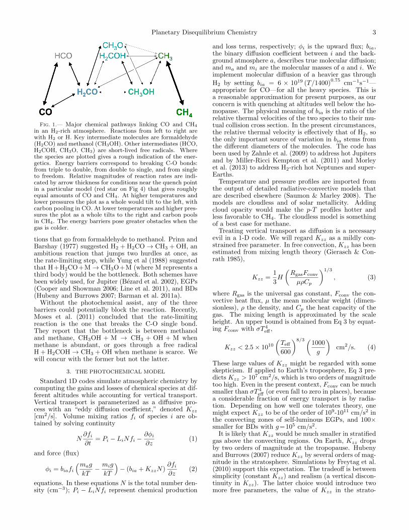
Figure 1 illustrates the most important chemical path-ways between CO and CH4 in a warm H2-rich atmo-sphere. The path from CO to CH4 climbs over threeenergy barriers, the first between CO and formaldehyde(H2CO), the second between formaldehyde and methanol(CH3OH), and the third between methanol and methane.The three barriers can be thought of as reducing theC≡O triple bond to a double bond, reducing the C=Odouble bond to a single bond, and splitting C from Oentirely.

In photochemistry the first barrier is unimportant be-cause atomic hydrogen is generated in abundances thatvastly exceed equilibrium (Liang et al. 2003). Kineticbarriers to adding H to CO to make HCO or addingH to HCO to make H2CO are insignificant. The thirdbarrier is unimportant in photochemistry because inci-dent UV radiation readily splits CH3OH into CH3 andOH, which is quickly followed by adding photochemicalH to CH3 to make CH4. In photochemistry the energyto overcome the first and third barriers comes from UVphotons.

By contrast, the middle barrier is not easily overcomeby photochemistry. Formaldehyde is readily photolyzedbut the products are either CO or HCO; i.e., regress thatleaves the C=O bond unbroken. Meanwhile successive3-body additions of photochemical H to H2CO to makeCH3OH face considerable kinetic barriers, save at hightemperatures where CH4 is not favored. The historicfocus of the planetary literature was therefore on reac-

Planetary Disequilibrium Chemistry 3

Fig. 1.— Major chemical pathways linking CO and CH4

in an H2-rich atmosphere. Reactions from left to right arewith H2 or H. Key intermediate molecules are formaldehyde(H2CO) and methanol (CH3OH). Other intermediates (HCO,H2COH, CH3O, CH3) are short-lived free radicals. Wherethe species are plotted gives a rough indication of the ener-getics. Energy barriers correspond to breaking C-O bonds:from triple to double, from double to single, and from singleto freedom. Relative magnitudes of reaction rates are indi-cated by arrow thickness for conditions near the quench pointin a particular model (red star on Fig 4) that gives roughlyequal amounts of CO and CH4. At higher temperatures andlower pressures the plot as a whole would tilt to the left, withcarbon pooling in CO. At lower temperatures and higher pres-sures the plot as a whole tilts to the right and carbon poolsin CH4. The energy barriers pose greater obstacles when thegas is colder.

tions that go from formaldehyde to methanol. Prinn andBarshay (1977) suggested H2 + H2CO→ CH3 + OH, anambitious reaction that jumps two hurdles at once, asthe rate-limiting step, while Yung et al (1988) suggestedthat H+H2CO+M→ CH3O+M (where M represents athird body) would be the bottleneck. Both schemes havebeen widely used, for Jupiter (Bezard et al. 2002), EGPs(Cooper and Showman 2006; Line et al. 2011), and BDs(Hubeny and Burrows 2007; Barman et al. 2011a).

Without the photochemical assist, any of the threebarriers could potentially block the reaction. Recently,Moses et al. (2011) concluded that the rate-limitingreaction is the one that breaks the C-O single bond.They report that the bottleneck is between methanoland methane, CH3OH + M → CH3 + OH + M whenmethane is abundant, or goes through a free radicalH + H2COH→ CH3 + OH when methane is scarce. Wewill concur with the former but not the latter.

3. THE PHOTOCHEMICAL MODEL

Standard 1D codes simulate atmospheric chemistry bycomputing the gains and losses of chemical species at dif-ferent altitudes while accounting for vertical transport.Vertical transport is parameterized as a diffusive pro-cess with an “eddy diffusion coefficient,” denoted Kzz

[cm2/s]. Volume mixing ratios fi of species i are ob-tained by solving continuity

N∂fi∂t

= Pi − LiNfi −∂φi∂z

(1)

and force (flux)

φi = biafi

(mag

kT− mig

kT

)− (bia +KzzN)

∂fi∂z

(2)

equations. In these equations N is the total number den-sity (cm−3); Pi − LiNfi represent chemical production

and loss terms, respectively; φi is the upward flux; bia,the binary diffusion coefficient between i and the back-ground atmosphere a, describes true molecular diffusion;and ma and mi are the molecular masses of a and i. Weimplement molecular diffusion of a heavier gas throughH2 by setting bia = 6 × 1019 (T/1400)

0.75cm−1s−1—

appropriate for CO—for all the heavy species. This isa reasonable approximation for present purposes, as ourconcern is with quenching at altitudes well below the ho-mopause. The physical meaning of bia is the ratio of therelative thermal velocities of the two species to their mu-tual collision cross section. In the present circumstances,the relative thermal velocity is effectively that of H2, sothe only important source of variation in bia stems fromthe different diameters of the molecules. The code hasbeen used by Zahnle et al. (2009) to address hot Jupitersand by Miller-Ricci Kempton et al. (2011) and Morleyet al. (2013) to address H2-rich hot Neptunes and super-Earths.

Temperature and pressure profiles are imported fromthe output of detailed radiative-convective models thatare described elsewhere (Saumon & Marley 2008). Themodels are cloudless and of solar metallicity. Addingcloud opacity would make the p-T profiles hotter andless favorable to CH4. The cloudless model is somethingof a best case for methane.

Treating vertical transport as diffusion is a necessaryevil in a 1-D code. We will regard Kzz as a mildly con-strained free parameter. In free convection, Kzz has beenestimated from mixing length theory (Gierasch & Con-rath 1985),

Kzz =1

3H

(RgasFconv

µρCp

)1/3

, (3)

where Rgas is the universal gas constant, Fconv the con-vective heat flux, µ the mean molecular weight (dimen-sionless), ρ the density, and Cp the heat capacity of thegas. The mixing length is approximated by the scaleheight. An upper bound is obtained from Eq 3 by equat-ing Fconv with σT 4

eff ,

Kzz < 2.5× 1010

(Teff

600

)8/3 (1000

g

)cm2/s. (4)

These large values of Kzz might be regarded with someskepticism. If applied to Earth’s troposphere, Eq 3 pre-dicts Kzz > 107 cm2/s, which is two orders of magnitudetoo high. Even in the present context, Fconv can be muchsmaller than σT 4

eff (or even fall to zero in places), becausea considerable fraction of energy transport is by radia-tion. Depending on how well one tolerates theory, onemight expect Kzz to be of the order of 109-1011 cm/s2 inthe convecting zones of self-luminous EGPs, and 100×smaller for BDs with g=105 cm/s2.

It is likely that Kzz would be much smaller in stratifiedgas above the convecting regions. On Earth, Kzz dropsby two orders of magnitude at the tropopause. Hubenyand Burrows (2007) reduce Kzz by several orders of mag-nitude in the stratosphere. Simulations by Freytag et al.(2010) support this expectation. The tradeoff is betweensimplicity (constant Kzz) and realism (a vertical discon-tinuity in Kzz). The latter choice would introduce twomore free parameters, the value of Kzz in the strato-

4 Zahnle & Marley

sphere (ill constrained) and the altitude of the disconti-nuity (reasonably well constrained, but results could besensitive to this). A two layer model also makes inter-preting the numerical results in terms of a quench ap-proximation less straightforward because there can bemore than one quench point. For this study we chooseto treat Kzz as constant with height, but vary it over arange wide enough to encompass all likely values.

The chemical system used here comprises 366 for-ward chemical reactions and 32 photolysis reactions of64 chemical species made of H, C, N, O, and S. Themost important missing species is probably methylamine,CH3NH2. Reaction rates when known are selected fromthe publicly available NIST database (http://kinetics.nist.gov/kinetics). Although many of the important re-actions have been measured in both directions in the lab(e.g., both CH4+H→ CH3+H2 and CH3+H2 → CH4+Hhave been heavily studied), in general one direction ismuch better characterized than the other. Thermody-namic data (enthalpies and entropies) are usually betterknown over a wider range of temperatures. Thus it is bet-ter to complement each specific reaction with its exactreverse, with the forward and reverse rates linked self-consistently by the thermodynamic data of the speciesinvolved. This way the transition from equilibrium tokinetically-controlled abundances is automatic. Equilib-rium is reached when all the important forward and re-verse reactions are fast compared to changes in the statevariables.

How this is done is fully explained by Visscher andMoses (2011). What follows is a telegraphic summary.For reactions of the form A + B → C + D with for-ward reaction rate kf , the reverse rate (i.e., the ratefor C + D → A + B) is kr = kf exp (−∆G/RT ), where∆G, the Gibbs free energy, is obtained from enthalpiesand entropies of the of the reactants and products,∆G = HA +HB −HC −HD − T (SA + SB − SC − SD).For associative reactions of the form A + B → AB,the rate for the reverse reaction (dissociation of AB)is kr = kf (kT/P◦) exp (−∆G/RT ), where P◦ = 106

dynes/cm2 is one atmosphere. Similarly, the associa-tive reverse of a dissociative reaction is given by kr =kf (P◦/kT ) exp (−∆G/RT ).

Thermodynamic data as a function of temper-ature are available for atoms and most smallmolecules from NIST in the form of empiricalShomate equation fits for enthalpy and entropy(http://webbook.nist.gov/chemistry/form-ser). Zeropoint data for HS are corrected by Lodders (2004). ForCH3OH and C2H6 we use heat capacities as a functionof temperature to derive Shomate equation fits for en-thalpy and entropy. Unfortunately, many of the moreexotic free radicals are not listed in the publicly avail-able NIST databases. For many of these we use estimatesgiven in Burcat and Ruscic (2005)’s widely available grayliterature compilation. For NNH we follow Haworth etal. (2003), and for N2H2 and N2H3 we follow Matuset al. (2006). Inaccurate thermodynamic data for freeradicals are not a problem for equilibrium calculationsof well-characterized abundant species because poorly-characterized free radicals are never abundant. On theother hand, poorly-characterized species do pose a prob-lem in disequilibrium kinetics because net reaction rates

depend on the uncertain abundances of free radicals,which are determined by their thermodynamic proper-ties.

The lower boundary is set deep enough that all speciesare in thermodynamic equilibrium. We find that pres-sures above 300 bars and temperatures above 2000 Kusually suffice, with the limiting species being N2. Theupper boundary condition is zero flux for all species. Weplace the upper boundary at ∼ 10−6 bars, as higheraltitudes require additional physics and chemistry (ionchemistry, thermospheric heating) that go beyond thescope of this work. Steady state solutions are found byintegrating the time-dependent chemical and transportequations through time using an overcorrected fully im-plicit backward-difference method. Most models take afew minutes to run to steady state from arbitrary initialconditions on a vintage laptop computer, although someparticular cases can be more challenging.

Photolysis significantly affects the composition of at-mospheres at very high altitudes even when the incidentUV flux is small. In our models we have set the incidentUV flux to 0.1% that at Earth. Photolysis plays almostno part at the higher pressures germane to quenching andis not further discussed here. We have not included thereverses of photolysis reactions (radiative attachment,e.g. OH + H→ H2O + hν) in detailed balancing. Recentwork has shown that radiative attachment can be im-portant in hydrocarbon growth in planetary atmosphereswhen the resulting molecule is complex enough that ra-diative relaxation can be effective (Vuitton et al. 2012).

3.1. Two examples

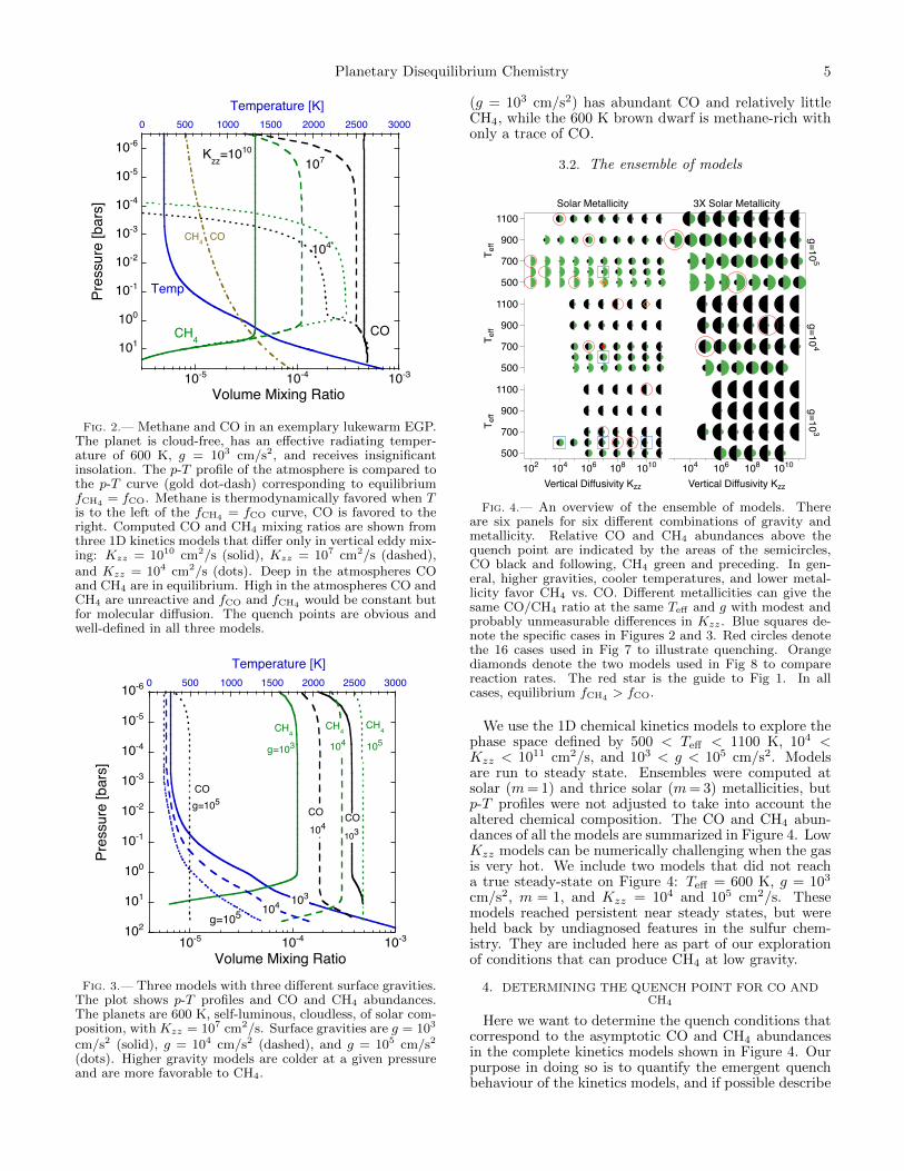
Figure 2 shows how Kzz effects chemistry on a tepid(Teff = 600 K), cloud-free, relatively low mass (g = 103

cm/s2) extrasolar planet of solar composition. Insolationis insignificant. Three different Kzz are compared. (i)Strong vertical mixing—Kzz = 1010 cm2/s—suppressesCH4 and maintains fCO � fCH4

to very high alti-tudes. CO and CH4 are in chemical equilibrium belowthe quench point at ∼ 4 bars and 1450 K. (ii) A moreJupiter-like Kzz = 107 cm2/s raises the quench point to1.5 bars and 1280 K, which is better for CH4. (iii) Weakmixing, Kzz = 104 cm2/s, raises the quench point to 0.6bars and 1000 K, which is cool enough, barely, to fall intothe CH4 field, so that fCH4 > fCO in this planet’s photo-sphere. The effect of molecular diffusion (in which heavymolecules sink through H2) is apparent above 3 × 10−6

bars at Kzz = 107 cm2/s and above 3 × 10−3 bars atKzz = 104 cm2/s.

At a given effective temperature, surface gravity de-termines whether the atmosphere is CO or CH4 domi-nated. Figure 3 shows CO and CH4 abundances in threeworlds that differ only in their surface gravities. Theatmospheres are cloud-free and of elementally solar com-position. The models shown here have effective radiat-ing temperatures of 600 K and a Jupiter-like Kzz = 107

cm2/s. Surface gravities range from a Saturn-like g = 103

cm/s2 to a brown-dwarf-like g = 105 cm/s2. The com-puted CO/CH4 ratio is sensitive to surface gravity. Thisis because the p-T profile is displaced to higher pres-sures and lower temperatures when gravity is higher.Quenching at higher pressures and lower temperaturesfavors CH4 over CO. The result is that the 600 K planet

Planetary Disequilibrium Chemistry 5

10-6

10-5

10-4

10-3

10-2

10-1

100

101

10-5 10-4 10-3

0 500 1000 1500 2000 2500 3000

Pres

sure

[bar

s]

Volume Mixing Ratio

Temperature [K]

COCH4

Temp

COCH4

107Kzz=1010

104

Fig. 2.— Methane and CO in an exemplary lukewarm EGP.The planet is cloud-free, has an effective radiating temper-ature of 600 K, g = 103 cm/s2, and receives insignificantinsolation. The p-T profile of the atmosphere is compared tothe p-T curve (gold dot-dash) corresponding to equilibriumfCH4 = fCO. Methane is thermodynamically favored when Tis to the left of the fCH4 = fCO curve, CO is favored to theright. Computed CO and CH4 mixing ratios are shown fromthree 1D kinetics models that differ only in vertical eddy mix-ing: Kzz = 1010 cm2/s (solid), Kzz = 107 cm2/s (dashed),and Kzz = 104 cm2/s (dots). Deep in the atmospheres COand CH4 are in equilibrium. High in the atmospheres CO andCH4 are unreactive and fCO and fCH4 would be constant butfor molecular diffusion. The quench points are obvious andwell-defined in all three models.

10-6

10-5

10-4

10-3

10-2

10-1

100

101

102

10-5 10-4 10-3

0 500 1000 1500 2000 2500 3000

Pres

sure

[bar

s]

Volume Mixing Ratio

Temperature [K]

CO

CH4

g=105 104 103

g=103

g=105

104

104

103

105

CO CO

CH4CH4

Fig. 3.— Three models with three different surface gravities.The plot shows p-T profiles and CO and CH4 abundances.The planets are 600 K, self-luminous, cloudless, of solar com-position, with Kzz = 107 cm2/s. Surface gravities are g = 103

cm/s2 (solid), g = 104 cm/s2 (dashed), and g = 105 cm/s2

(dots). Higher gravity models are colder at a given pressureand are more favorable to CH4.

(g = 103 cm/s2) has abundant CO and relatively littleCH4, while the 600 K brown dwarf is methane-rich withonly a trace of CO.

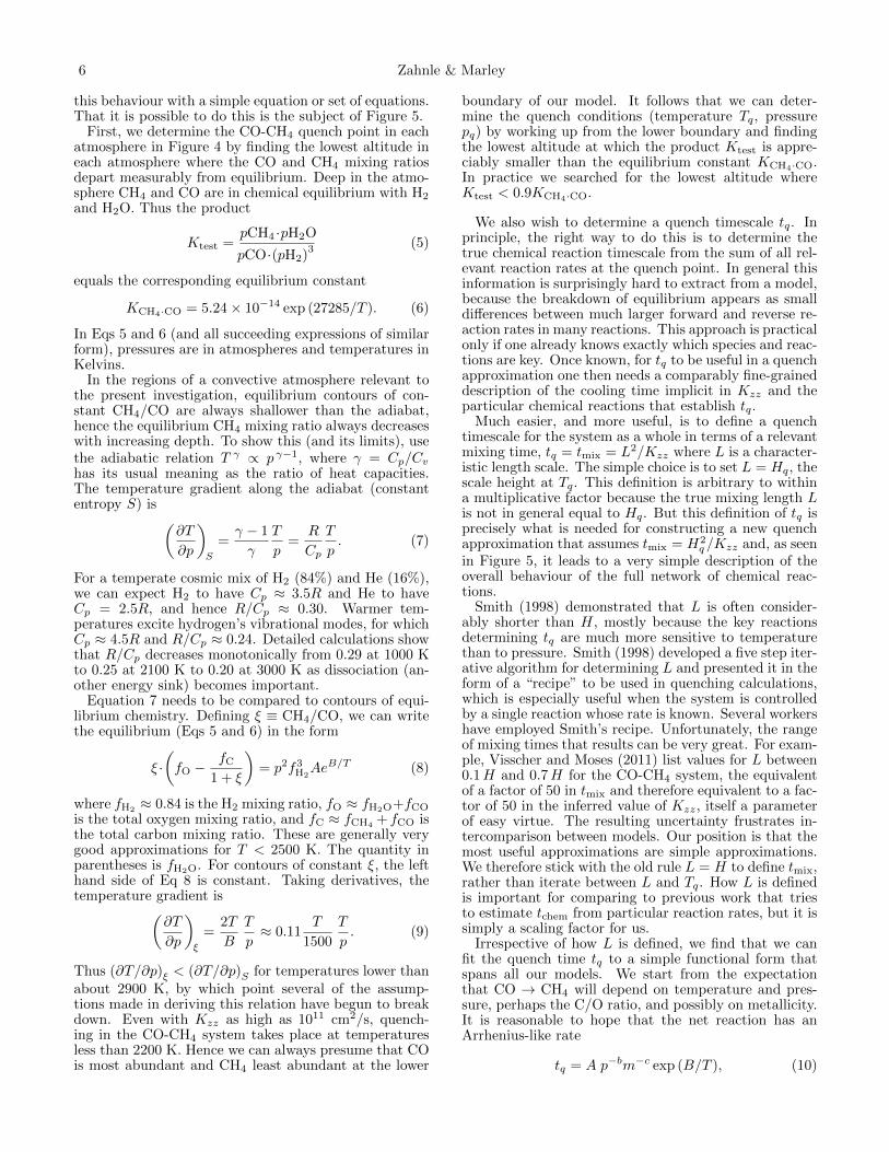
3.2. The ensemble of models

Solar Metallicity 3X Solar Metallicity

g=105

g=104

g=103T e

ff

500

700

900

1100

T eff

500

700

900

1100

T eff

500

700

900

1100

Vertical Diffusivity Kzz

102 104 106 108 1010

Vertical Diffusivity Kzz

104 106 108 1010

Fig. 4.— An overview of the ensemble of models. Thereare six panels for six different combinations of gravity andmetallicity. Relative CO and CH4 abundances above thequench point are indicated by the areas of the semicircles,CO black and following, CH4 green and preceding. In gen-eral, higher gravities, cooler temperatures, and lower metal-licity favor CH4 vs. CO. Different metallicities can give thesame CO/CH4 ratio at the same Teff and g with modest andprobably unmeasurable differences in Kzz. Blue squares de-note the specific cases in Figures 2 and 3. Red circles denotethe 16 cases used in Fig 7 to illustrate quenching. Orangediamonds denote the two models used in Fig 8 to comparereaction rates. The red star is the guide to Fig 1. In allcases, equilibrium fCH4 > fCO.

We use the 1D chemical kinetics models to explore thephase space defined by 500 < Teff < 1100 K, 104 <Kzz < 1011 cm2/s, and 103 < g < 105 cm/s2. Modelsare run to steady state. Ensembles were computed atsolar (m= 1) and thrice solar (m= 3) metallicities, butp-T profiles were not adjusted to take into account thealtered chemical composition. The CO and CH4 abun-dances of all the models are summarized in Figure 4. LowKzz models can be numerically challenging when the gasis very hot. We include two models that did not reacha true steady-state on Figure 4: Teff = 600 K, g = 103

cm/s2, m = 1, and Kzz = 104 and 105 cm2/s. Thesemodels reached persistent near steady states, but wereheld back by undiagnosed features in the sulfur chem-istry. They are included here as part of our explorationof conditions that can produce CH4 at low gravity.

4. DETERMINING THE QUENCH POINT FOR CO ANDCH4

Here we want to determine the quench conditions thatcorrespond to the asymptotic CO and CH4 abundancesin the complete kinetics models shown in Figure 4. Ourpurpose in doing so is to quantify the emergent quenchbehaviour of the kinetics models, and if possible describe

6 Zahnle & Marley

this behaviour with a simple equation or set of equations.That it is possible to do this is the subject of Figure 5.

First, we determine the CO-CH4 quench point in eachatmosphere in Figure 4 by finding the lowest altitude ineach atmosphere where the CO and CH4 mixing ratiosdepart measurably from equilibrium. Deep in the atmo-sphere CH4 and CO are in chemical equilibrium with H2

and H2O. Thus the product

Ktest =pCH4 ·pH2O

pCO·(pH2)3 (5)

equals the corresponding equilibrium constant

KCH4·CO = 5.24× 10−14 exp (27285/T ). (6)

In Eqs 5 and 6 (and all succeeding expressions of similarform), pressures are in atmospheres and temperatures inKelvins.

In the regions of a convective atmosphere relevant tothe present investigation, equilibrium contours of con-stant CH4/CO are always shallower than the adiabat,hence the equilibrium CH4 mixing ratio always decreaseswith increasing depth. To show this (and its limits), usethe adiabatic relation T γ ∝ p γ−1, where γ = Cp/Cvhas its usual meaning as the ratio of heat capacities.The temperature gradient along the adiabat (constantentropy S) is (

∂T

∂p

)S

=γ − 1

γ

T

p=

R

Cp

T

p. (7)

For a temperate cosmic mix of H2 (84%) and He (16%),we can expect H2 to have Cp ≈ 3.5R and He to haveCp = 2.5R, and hence R/Cp ≈ 0.30. Warmer tem-peratures excite hydrogen’s vibrational modes, for whichCp ≈ 4.5R and R/Cp ≈ 0.24. Detailed calculations showthat R/Cp decreases monotonically from 0.29 at 1000 Kto 0.25 at 2100 K to 0.20 at 3000 K as dissociation (an-other energy sink) becomes important.

Equation 7 needs to be compared to contours of equi-librium chemistry. Defining ξ ≡ CH4/CO, we can writethe equilibrium (Eqs 5 and 6) in the form

ξ ·(fO −

fC

1 + ξ

)= p2f3

H2AeB/T (8)

where fH2 ≈ 0.84 is the H2 mixing ratio, fO ≈ fH2O+fCO

is the total oxygen mixing ratio, and fC ≈ fCH4+ fCO is

the total carbon mixing ratio. These are generally verygood approximations for T < 2500 K. The quantity inparentheses is fH2O. For contours of constant ξ, the lefthand side of Eq 8 is constant. Taking derivatives, thetemperature gradient is(

∂T

∂p

)ξ

=2T

B

T

p≈ 0.11

T

1500

T

p. (9)

Thus (∂T/∂p)ξ < (∂T/∂p)S for temperatures lower thanabout 2900 K, by which point several of the assump-tions made in deriving this relation have begun to breakdown. Even with Kzz as high as 1011 cm2/s, quench-ing in the CO-CH4 system takes place at temperaturesless than 2200 K. Hence we can always presume that COis most abundant and CH4 least abundant at the lower

boundary of our model. It follows that we can deter-mine the quench conditions (temperature Tq, pressurepq) by working up from the lower boundary and findingthe lowest altitude at which the product Ktest is appre-ciably smaller than the equilibrium constant KCH4·CO.In practice we searched for the lowest altitude whereKtest < 0.9KCH4·CO.

We also wish to determine a quench timescale tq. Inprinciple, the right way to do this is to determine thetrue chemical reaction timescale from the sum of all rel-evant reaction rates at the quench point. In general thisinformation is surprisingly hard to extract from a model,because the breakdown of equilibrium appears as smalldifferences between much larger forward and reverse re-action rates in many reactions. This approach is practicalonly if one already knows exactly which species and reac-tions are key. Once known, for tq to be useful in a quenchapproximation one then needs a comparably fine-graineddescription of the cooling time implicit in Kzz and theparticular chemical reactions that establish tq.

Much easier, and more useful, is to define a quenchtimescale for the system as a whole in terms of a relevantmixing time, tq = tmix = L2/Kzz where L is a character-istic length scale. The simple choice is to set L = Hq, thescale height at Tq. This definition is arbitrary to withina multiplicative factor because the true mixing length Lis not in general equal to Hq. But this definition of tq isprecisely what is needed for constructing a new quenchapproximation that assumes tmix = H2

q /Kzz and, as seenin Figure 5, it leads to a very simple description of theoverall behaviour of the full network of chemical reac-tions.

Smith (1998) demonstrated that L is often consider-ably shorter than H, mostly because the key reactionsdetermining tq are much more sensitive to temperaturethan to pressure. Smith (1998) developed a five step iter-ative algorithm for determining L and presented it in theform of a “recipe” to be used in quenching calculations,which is especially useful when the system is controlledby a single reaction whose rate is known. Several workershave employed Smith’s recipe. Unfortunately, the rangeof mixing times that results can be very great. For exam-ple, Visscher and Moses (2011) list values for L between0.1H and 0.7H for the CO-CH4 system, the equivalentof a factor of 50 in tmix and therefore equivalent to a fac-tor of 50 in the inferred value of Kzz, itself a parameterof easy virtue. The resulting uncertainty frustrates in-tercomparison between models. Our position is that themost useful approximations are simple approximations.We therefore stick with the old rule L = H to define tmix,rather than iterate between L and Tq. How L is definedis important for comparing to previous work that triesto estimate tchem from particular reaction rates, but it issimply a scaling factor for us.

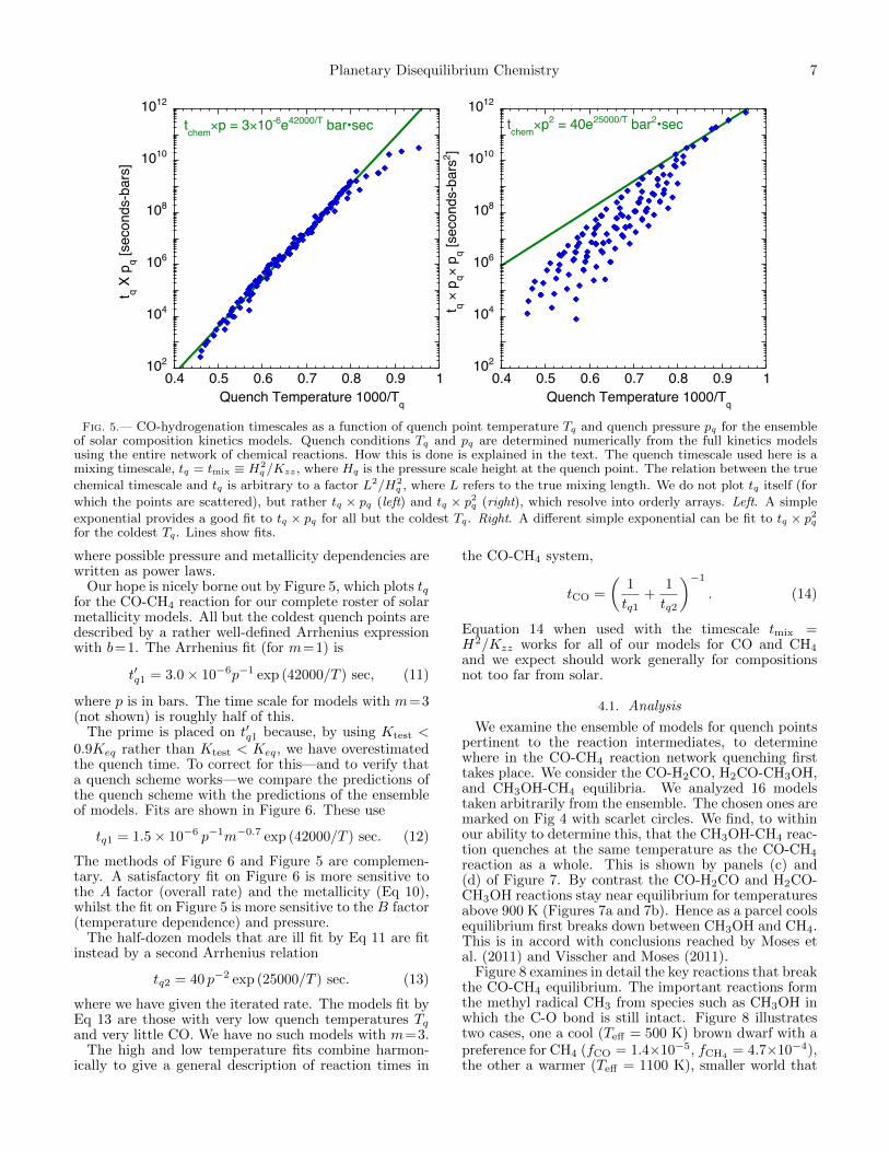
Irrespective of how L is defined, we find that we canfit the quench time tq to a simple functional form thatspans all our models. We start from the expectationthat CO → CH4 will depend on temperature and pres-sure, perhaps the C/O ratio, and possibly on metallicity.It is reasonable to hope that the net reaction has anArrhenius-like rate

tq = A p−bm−c exp (B/T ), (10)

Planetary Disequilibrium Chemistry 7

102

104

106

108

1010

1012

0.4 0.5 0.6 0.7 0.8 0.9 1

t q × p

q× p

q [sec

onds

-bar

s2 ]

Quench Temperature 1000/Tq

tchem×p2 = 40e25000/T bar2•sec

102

104

106

108

1010

1012

0.4 0.5 0.6 0.7 0.8 0.9 1

t q X p

q [sec

onds

-bar

s]

Quench Temperature 1000/Tq

tchem×p = 3×10-6e42000/T bar•sec

Fig. 5.— CO-hydrogenation timescales as a function of quench point temperature Tq and quench pressure pq for the ensembleof solar composition kinetics models. Quench conditions Tq and pq are determined numerically from the full kinetics modelsusing the entire network of chemical reactions. How this is done is explained in the text. The quench timescale used here is amixing timescale, tq = tmix ≡ H2

q /Kzz, where Hq is the pressure scale height at the quench point. The relation between the true

chemical timescale and tq is arbitrary to a factor L2/H2q , where L refers to the true mixing length. We do not plot tq itself (for

which the points are scattered), but rather tq × pq (left) and tq × p2q (right), which resolve into orderly arrays. Left. A simple

exponential provides a good fit to tq × pq for all but the coldest Tq. Right. A different simple exponential can be fit to tq × p2q

for the coldest Tq. Lines show fits.

where possible pressure and metallicity dependencies arewritten as power laws.

Our hope is nicely borne out by Figure 5, which plots tqfor the CO-CH4 reaction for our complete roster of solarmetallicity models. All but the coldest quench points aredescribed by a rather well-defined Arrhenius expressionwith b=1. The Arrhenius fit (for m=1) is

t′q1 = 3.0× 10−6p−1 exp (42000/T ) sec, (11)

where p is in bars. The time scale for models with m=3(not shown) is roughly half of this.

The prime is placed on t′q1 because, by using Ktest <0.9Keq rather than Ktest < Keq, we have overestimatedthe quench time. To correct for this—and to verify thata quench scheme works—we compare the predictions ofthe quench scheme with the predictions of the ensembleof models. Fits are shown in Figure 6. These use

tq1 = 1.5× 10−6 p−1m−0.7 exp (42000/T ) sec. (12)

The methods of Figure 6 and Figure 5 are complemen-tary. A satisfactory fit on Figure 6 is more sensitive tothe A factor (overall rate) and the metallicity (Eq 10),whilst the fit on Figure 5 is more sensitive to the B factor(temperature dependence) and pressure.

The half-dozen models that are ill fit by Eq 11 are fitinstead by a second Arrhenius relation

tq2 = 40 p−2 exp (25000/T ) sec. (13)

where we have given the iterated rate. The models fit byEq 13 are those with very low quench temperatures Tqand very little CO. We have no such models with m=3.

The high and low temperature fits combine harmon-ically to give a general description of reaction times in

the CO-CH4 system,

tCO =

(1

tq1+

1

tq2

)−1

. (14)

Equation 14 when used with the timescale tmix =H2/Kzz works for all of our models for CO and CH4

and we expect should work generally for compositionsnot too far from solar.

4.1. Analysis

We examine the ensemble of models for quench pointspertinent to the reaction intermediates, to determinewhere in the CO-CH4 reaction network quenching firsttakes place. We consider the CO-H2CO, H2CO-CH3OH,and CH3OH-CH4 equilibria. We analyzed 16 modelstaken arbitrarily from the ensemble. The chosen ones aremarked on Fig 4 with scarlet circles. We find, to withinour ability to determine this, that the CH3OH-CH4 reac-tion quenches at the same temperature as the CO-CH4

reaction as a whole. This is shown by panels (c) and(d) of Figure 7. By contrast the CO-H2CO and H2CO-CH3OH reactions stay near equilibrium for temperaturesabove 900 K (Figures 7a and 7b). Hence as a parcel coolsequilibrium first breaks down between CH3OH and CH4.This is in accord with conclusions reached by Moses etal. (2011) and Visscher and Moses (2011).

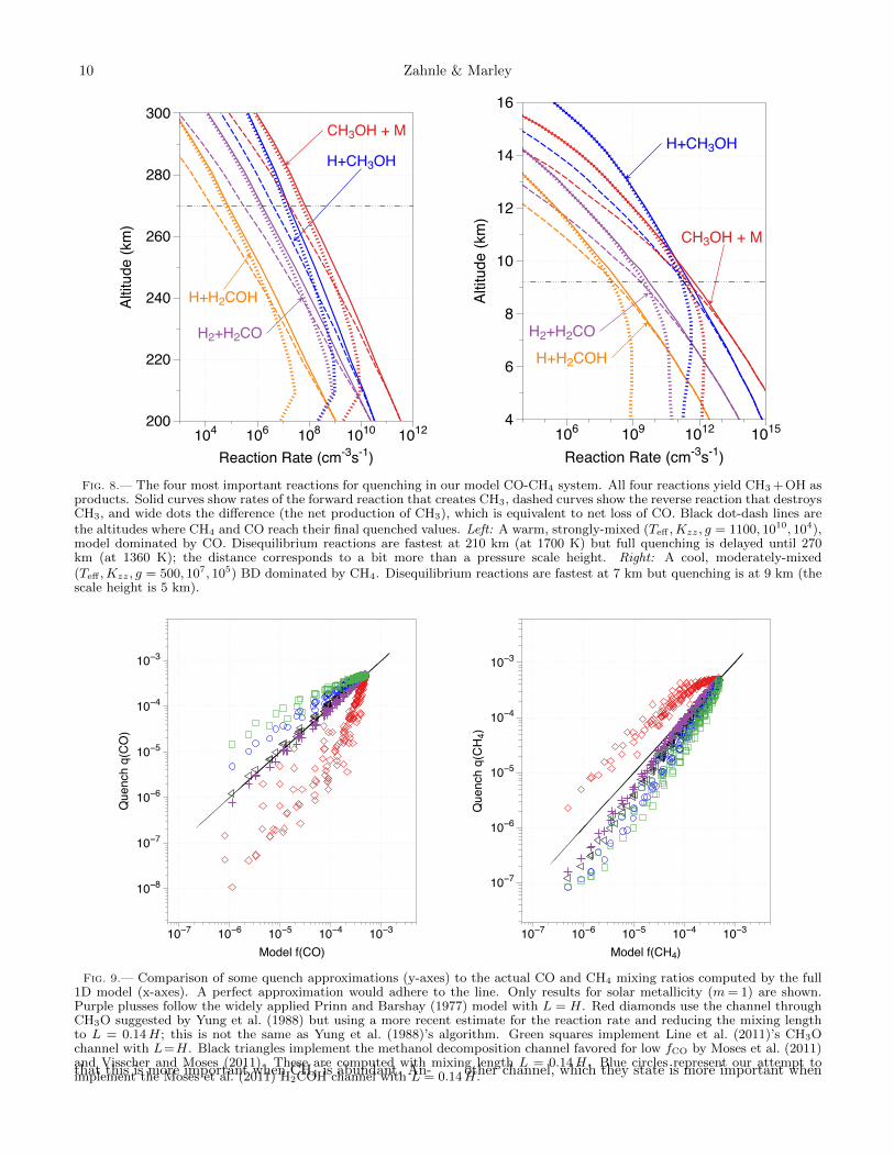
Figure 8 examines in detail the key reactions that breakthe CO-CH4 equilibrium. The important reactions formthe methyl radical CH3 from species such as CH3OH inwhich the C-O bond is still intact. Figure 8 illustratestwo cases, one a cool (Teff = 500 K) brown dwarf with apreference for CH4 (fCO = 1.4×10−5, fCH4

= 4.7×10−4),the other a warmer (Teff = 1100 K), smaller world that

8 Zahnle & Marley

10-7

10-6

10-5

10-4

10-3

10-7 10-6 10-5 10-4 10-3

Que

nch

Mix

ing

Rat

io f(

CO

)

Model Mixing Ratio f(CO)

10-7

10-6

10-5

10-4

10-3

10-7 10-6 10-5 10-4 10-3

Que

nch

Mix

ing

Rat

io f(

CH

4)

Model Mixing Ratio f(CH4)

Fig. 6.— CO (left) and CH4 (right) mixing ratios predicted by the quenching approximation tchem = tmix (y-axis) plotted againstthe actual asymptotic mixing ratio determined from the full ensemble of 1-D kinetics model (x-axis). A perfect approximationwould adhere to the line. Open red symbols are for m=1 and solid black symbols are for m=3 using Eq 12.

favors CO (fCO = 4.8× 10−4, fCH4= 1.0× 10−5). Both

models assume solar metallicity (m= 1). In both casesthe most important reaction is simple thermal decompo-sition of methanol, CH3OH + M→ CH3 + OH, althoughthe reaction of methanol with atomic hydrogen is nearlyas fast in the colder, higher gravity case. The reactionH2COH+H, which Moses et al. (2011) report as the mostimportant in their CO-rich models, does not appear tobe very important in ours. We do not claim that our sys-tem is better; we merely point out that abundances andreaction rates of furtive species like H2COH are highlyuncertain.

4.2. Comparisons with previous work

To put our results in perspective, we compare themto some quench approximations seen in the literature.Published quench approximations begin by identifying aparticular forward reaction as the bottleneck and thencalculate CO loss time scales from the chosen reaction’srate; variety lies in the reactions that are chosen and thereaction rates adopted.

We begin with the classic Prinn and Barshay (1977)prescription, used by Hubeny and Burrows (2007) astheir “slow” case. Prinn and Barshay (1977) suggested

H2 + H2CO→ CH3 + OH (15)

as a rate-limiting reaction, with reaction rate kf = 2.3×10−10e−36200/T cm3/s. R15 is a reaction that jumps overtwo energy barriers in Figure 1, which makes it look likeit should be relatively unlikely. Figure 8 shows that R15is modestly important in our system, but we use a newerslower rate estimated by Jasper et al (2007). The timeconstant for CO loss by reaction R15 using Prinn andBarshay (1977)’s rate is approximated by the forwardreaction

t−1chem =

−1

[CO]

∂ [CO]

∂t=kf [H2] [H2CO]

[CO]sec−1 (16)

where the notation [CO] refers to number density [cm−3].

To evaluate tchem for R15, we put formaldehyde in equi-librium with CO and H2,

pH2CO

pH2 ·pCO= KH2CO = 3.3× 10−7 exp (1420/T ), (17)

to obtain

tchem =1.3× 1016 exp (34780/T )

pNf2H2

sec. (18)

The number density N is related to the pressure p inbars by NkT =106 p. The predictions of Eq 18 are com-pared to results from our complete models in Figure 9.Equation 18 works quite well in a quench approximationto our full model, especially for cases where CH4 is pre-dicted to be abundant, despite its being based on thewrong reaction with the wrong rate. As the Prinn andBarshay (1977) approximation has been widely used fora very long time, it is valuable to see that it seems towork rather well. When compared to Eq 12, Eq 18 hasa stronger pressure dependence (p−2 vs. p−1), a weakertemperature dependence (T ·e34780/T vs. e42000/T ), andno dependence on metallicity.

More recent discussions of the CO-CH4 quench approx-imation omit enough details that they can be challengingto reproduce. We attempt to do so here because the com-parisons are illuminating. Yung et al. (1988) suggestedthat the rate-limiting step is the 3-body reaction

H + H2CO + M→ CH3O + M. (19)

Hubeny and Burrows (2007) use R19 as their “fast” ratewith L = H. Barman et al. (2011a) also use this rate,but following Smith (1998) they set the mixing length Lto unspecified values between 10% to 20% of the scaleheight, which effectively slows the “fast” rate by a factorof 25-100 compared to L = H. Cooper and Showman(2006) implemented the CH3O channel with a differentreaction rate while following Smith’s “recipe.” We usethe asymptotic high pressure rate

Planetary Disequilibrium Chemistry 9

10-6

10-5

10-4

600 800 1000 1200

K =p

H2C

O /p

H2/

pCO

Temperature

equilibrium

CO + H2 ↔ H2CO

(a)

10-6

10-5

10-4

10-3

10-2

800 1000 1200 1400 1600 1800 2000

K =

pCH

3OH

* pH

2 / p

CH

4 /p

H2O

Temperature K

equilibrium

CH3OH + H2 ↔ CH4 + H2O

(c)

10-4

10-3

10-2

10-1

100

101

102

103

500 1000 1500 2000

K =

pCH

3OH

/ pH

2CO

/pH

2

Temperature K

equilibrium

H2CO + H2 ↔ CH3OH

(b)

10-8

10-6

10-4

10-2

100

102

104

800 1000 1200 1400 1600 1800 2000

K =

pCH

4 * p

H2O

/ pC

O /p

H23

Temperature K

equilibrium

CO + 3H2 ↔ CH4 + H2O

(d)

Fig. 7.— Quenching behavior of the three intermediate reactions (a, b, c) and of the CO↔ CH4 system as a whole (d). Resultsare shown from 16 models chosen to provide a representative sample of the ensemble (marked by red circles in Fig. 4). Panels(a,b) show that CO↔ H2CO and H2CO↔ CH3OH appear to be equilibrated in all models at T > 900 K. Panel (c) shows thatequilibration of CH3OH and CH4 is more difficult. In detail the quench points for CH3OH ↔ CH4 appear to be the same asthe quench points for CO ↔ CH4 as shown in panel (d) for the same 16 models. Evidently the bottleneck is between CH3OHand CH4, in accord with conclusions reached by Moses et al (2011).

k∞ = 8.0× 10−10 exp (−3160/T ),a very fast rate which we obtained by reversing the

first order rate for CH3O → H + H2CO given by Rauket al. (2003). If we presume that H and H2CO are bothin equilibrium, we can use the hydrogen equilibrium con-stant KH·H2 = 1155 e−26916/T = pH · pH−0.5

2 to obtain

t−1chem =

k∞ [H] [H2CO]

[CO]= k∞ p1.5 f1.5

H2

(106

kT

)KH2COKH·H2 .

(20)Evaluated,

tchem = 4.5× 10−10 Tp−1.5f−1.5H2

exp (28656/T ). (21)

Results of using Eq 21 are shown as red diamonds on Fig9 with L = 0.14H, which is comparable to what Barmanet al. (2011a) use (the fit would look worse with L = H).These stand out with too much CH4 and too little CO,because R19 is not a true bottleneck.

Line et al. (2011) moved the bottleneck to CH3O +H2 → CH3OH + H. To compute a rate constant, weuse pCH3O = KCH3O ·pH2 ·pH ·pCO, where KCH3O =

3.0 × 10−11e10582/T is the relevant equilibrium constant(the large number of significant digits in these equilib-rium constants do not imply accuracy). To completethe equation we also assume that H and H2 are in equi-librium. We use the reaction rate given by Line et al.(2011), which results in

tchem =1.2× 1029 exp (45720/T )

T 4Npf2H2

sec. (22)

Results are shown as green squares on Figure 9 usingL = H, as Line et al. (2011) do. Because it predicts toomuch CO and too little CH4, tchem given by Eq 22 is tooslow.

Based on detailed analysis of the reactions in a com-plete 1D model similar to our own, Moses et al. (2011)concluded that the bottleneck is associated with break-ing the C-O bond. They propose several key channels.One channel is thermal decomposition of methanol,

CH3OH + M→ CH3 + OH + M. (23)

Visscher and Moses (2011) and Moses et al. (2011) state

10 Zahnle & Marley

H+CH3OH

H+H2COH

CH3OH + M

H2+H2CO

Altit

ude

(km

)

200

220

240

260

280

300

Reaction Rate (cm-3s-1)104 106 108 1010 1012

H+CH3OH

H+H2COH

CH3OH + M

H2+H2CO

Altit

ude

(km

)

4

6

8

10

12

14

16

Reaction Rate (cm-3s-1)106 109 1012 1015

Fig. 8.— The four most important reactions for quenching in our model CO-CH4 system. All four reactions yield CH3 +OH asproducts. Solid curves show rates of the forward reaction that creates CH3, dashed curves show the reverse reaction that destroysCH3, and wide dots the difference (the net production of CH3), which is equivalent to net loss of CO. Black dot-dash lines arethe altitudes where CH4 and CO reach their final quenched values. Left: A warm, strongly-mixed (Teff ,Kzz, g = 1100, 1010, 104),model dominated by CO. Disequilibrium reactions are fastest at 210 km (at 1700 K) but full quenching is delayed until 270km (at 1360 K); the distance corresponds to a bit more than a pressure scale height. Right: A cool, moderately-mixed(Teff ,Kzz, g = 500, 107, 105) BD dominated by CH4. Disequilibrium reactions are fastest at 7 km but quenching is at 9 km (thescale height is 5 km).

Que

nch

q(C

O)

10−8

10−7

10−6

10−5

10−4

10−3

Model f(CO)10−7 10−6 10−5 10−4 10−3

Que

nch

q(C

H4)

10−7

10−6

10−5

10−4

10−3

Model f(CH4)10−7 10−6 10−5 10−4 10−3

Fig. 9.— Comparison of some quench approximations (y-axes) to the actual CO and CH4 mixing ratios computed by the full1D model (x-axes). A perfect approximation would adhere to the line. Only results for solar metallicity (m= 1) are shown.Purple plusses follow the widely applied Prinn and Barshay (1977) model with L = H. Red diamonds use the channel throughCH3O suggested by Yung et al. (1988) but using a more recent estimate for the reaction rate and reducing the mixing lengthto L = 0.14H; this is not the same as Yung et al. (1988)’s algorithm. Green squares implement Line et al. (2011)’s CH3Ochannel with L=H. Black triangles implement the methanol decomposition channel favored for low fCO by Moses et al. (2011)and Visscher and Moses (2011). These are computed with mixing length L = 0.14H. Blue circles represent our attempt toimplement the Moses et al. (2011) H2COH channel with L = 0.14H.that this is more important when CH4 is abundant. An- other channel, which they state is more important when

Planetary Disequilibrium Chemistry 11

CO� CH4, is

CH2OH + H→ CH3 + OH. (24)

The rate of R24 depends on the uncertain thermody-namic properties of CH2OH. In the high pressure limit,methanol decomposition R23 is a first order reaction,

∂ [CH3OH]

∂t= −k∞ [CH3OH] . (25)

Jasper et al (2007) estimate k∞ from theory

k∞ = 6.251× 1016 (300/T )0.6148

exp (−46573/T ) sec−1.

The methanol equilibrium constant

KCH3OH =pCH3OH

pCO · pH22

= 1.1× 10−13e13000/T

relates [CH3OH] to [CO]. The reaction timescale is then

tchem =(k∞pH

22KCH3OH

)−1

= 4.4× 10−6 T 0.6148 exp (33573/T ) p−2f−2H2

sec.(26)

Equation 26 has a weaker dependence on T , a strongerdependence on p than we find for the ensemble, and nodependence on metallicity.

Figure 9 illustrates quenching using Eq 26 as blacktriangles. For the comparison we take L = 0.14H. Thisapproximates what Moses et al. (2011) may be using.Equation 26 does well, especially in cases where CO �CH4 at quenching, which is the regime for which Moseset al. (2011) report that Eq 26 applies. Equation 26 doesbetter if L > 0.14H. The match is best for CO withL = 0.2H, and better for CH4 with L≈0.5H.

To reconstruct a simple form for the H2COH chan-nel, we need to estimate the equilibrium abundance ofH2COH. We use pH2COH = KH2COH · pH2 · pH · pCOwith KH2COH = 1.0× 10−12e15843/T . We assume that Hand H2 are in equilibrium. Jasper et al. (2007) list a fastrate, k = 2.8 × 10−10 cm3/s, for the reaction of H andH2COH. Assembling the parts, we obtain

tchem =2.7× 1015 exp (38000/T )

Npf−2H2

sec. (27)

Results are shown as blue circles on Figure 9. Equation27 has a similar T dependence to what we find for thesystem as a whole, but the overall rate is about 3 ordersof magnitude slower using L = 0.14H, or about ten timesslower using L = H.

Disagreement between our model and Moses et al overthe H2COH channel is also apparent in Figure 8. TheH2COH radical plays a much more modest role in our1-D code than it does in Moses et al. (2011)’s. The sameis true for CH3O. Why this should be so is likely relatedto differing guesses of H2COH’s and CH3O’s ill-knownthermodynamic properties.

There are some more subtle differences between ourmodel and previous quench models that should be noted.One is that we find tchem ∝ p−1 by fitting to the en-semble, whilst quench models that attempt to identifythe one key forward reaction tend to get tchem ∝ p−2.This difference is the reason why quench prescriptions inFigure 9 that do well with fCO � fCH4 miss the mark

somewhat with fCH4� fCO. Figure 6 that uses tq ∝ p−1

shows fine agreement at both ends of the scale.Another difference is that we see a well-defined metal-

licity dependence when fitting to the ensemble. Themetallicity dependence probably stems from the reversereaction, which as noted is usually ignored. As equilib-rium breaks down, the reaction slows in both directions,more quickly in the reverse direction than in the forwarddirection. This behavior is shown clearly in Figure 8,where forward, reverse, and net reaction rates are plot-ted. It is the net reaction, the difference between theforward and reverse reactions, that defines the retreatfrom equilibrium, not the forward reaction alone. Forexample, the time scale for the methanol decompositionchannel is

t−1net =

−1

[CO]

∂ [CO]

∂t=kf [CH3OH]

[CO]− kr [CH3] [OH]

[CO].

(28)The reverse reaction is quadratic in metallicity, whilst[CO] is quadratic in metallicity only for fCO � fCH4

,which suggests that it is through the reverse reaction thatmetallicity enters tCO. The same consideration appliesfor all the important reactions in Figure 8, as the reversereaction in every case is between CH3 and OH.

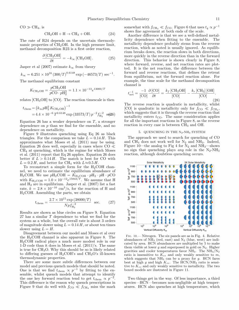
5. QUENCHING IN THE N2-NH3 SYSTEM

The approach we used to search for quenching of COand CH4 does not work well for N2 and NH3. Indeed,Figure 10—the analog to Fig 4 for N2 and NH3—showsno sign that quenching plays any role in the N2-NH3

reaction, although doubtless quenching occurs.

Solar Metallicity 3X Solar Metallicity

Teff

g=1

03

500

700

900

1100

Teff

g=1

04

500

700

900

1100

Teff

g=1

05

500

700

900

1100

Vertical Diffusivity Kzz

103 106 109

Vertical Diffusivity Kzz

104 106 108 1010

Fig. 10.— Nitrogen. The six panels are as in Fig. 4. Relativeabundances of NH3 (red, east) and N2 (blue, west) are indi-cated by area. HCN abundances are multiplied by 5 to makethem visible at lower g and superposed in gold on N2. Highergravities and cooler temperatures favor NH3. The NH3/N2

ratio is insensitive to Kzz and only weakly sensitive to m,which suggests that NH3 can be a proxy for g. HCN faresbest at high g and high Kzz. The HCN/NH3 ratio is sensi-tive to Kzz and only weakly sensitive to metallicity. The twoboxed models are ilustrated in Figure 11.

Two things get in the way. Of less importance, a thirdspecies—HCN—becomes non-negligible at high temper-atures. HCN also quenches at high temperature, which

12 Zahnle & Marley

leaves the nitrogen system with three possibly distinctquench points: NH3-N2, NH3-HCN, and N2-HCN. Al-though HCN is never very abundant in equilibrium, itis often abundant enough that its decomposition can in-crease the NH3 abundance by more than 10% after theNH3-N2 reaction has quenched. When confused with thesecond, greater obstacle, HCN can make it difficult topinpoint where quenching occurs.

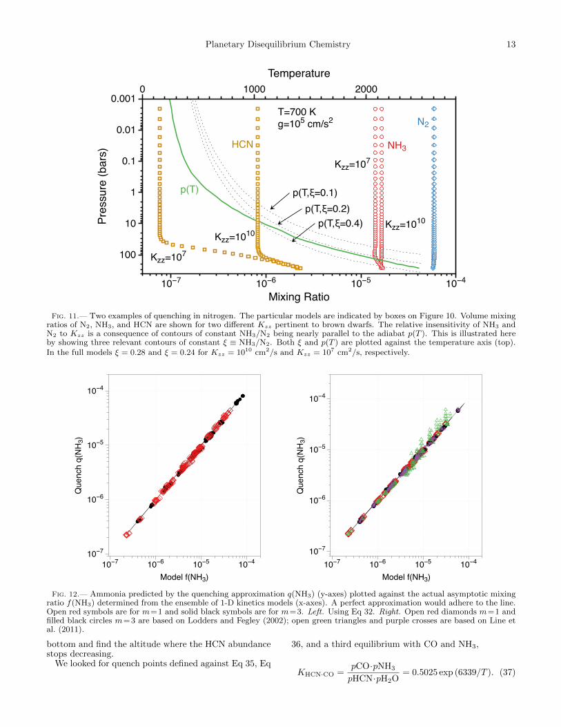
The greater obstacle is that curves of constant NH3/N2

are nearly parallel to the adiabat at the pressures andtemperatures where quenching occurs. This is illustatedin Figure 11. Consequently the NH3/N2 ratio in a par-cel remains close to equilibrium well after quenching hastaken place, which makes the NH3/N2 ratio indifferentto quenching (Saumon et al. 2006). To show this, writethe N2-NH3 equilibrium in the form

KNH3·N2= 5.90× 10−13 exp (13207/T ) =

pNH23

pN2 ·pH32

.

(29)Define ξ ≡ NH3/N2. If we approximate the total mixingratio of N by fN ≈ fNH3 + 2fN2 (including HCN makesthis very complicated), we can write

ξ2

(fN

2 + ξ

)= p2f3

H2AeB/T . (30)

With context-obvious substitutions, the temperaturegradient for contours of constant ξ is(

dT

dp

)ξ

=2T

B

T

p≈ 0.23

T

1500

T

p. (31)

The temperature gradient in Eq 31 is parallel to the adi-abat (Eq 7) at 1750 K, and nearly parallel for 1500 <T < 2000 K. For temperatures initially greater than1750 K, the equilibrium ratio of NH3/N2 decreases asthe parcel cools, reaching a minimum at ∼1750 K where(dT/dp)ξ = (dT/dp)S . If the parcel remains in chemi-

cal equilibrium, NH3/N2 will increase again as it coolsfurther. This then is how we explain the insensitivityof NH3/N2 to Kzz seen in Figure 10: the NH3/N2 ratiocomputed by the full kinetics model is near the equilib-rium value at the temperature where contours of NH3/N2

are parallel to the adiabat, which is also the minimumequilibrium value in the atmosphere. For the kinds ofatmospheres considered in this paper, it appears thatthe amount of ammonia in the visible parts of the atmo-sphere will be comparable to the minimum equilibriumabundance computed along the adiabat.

On the other hand, because our results are insensi-tive to quenching, it is not difficult to find a non-uniquechemical reaction time scale for the nitrogen system thatpredicts fNH3 well. A chemical reaction time scale thatworks well in a quenching scheme that sets the reactionrate time tNH3 equal to the mixing time tmix = H2/Kzz

is

tNH3= 1.0× 10−7p−1 exp (52000/T ) sec. (32)

This particular choice presumes that the energy barrieris set by N2 + H2 → NNH + H. This choice of tNH3

isnot unique. Almost any plausible choice of Arrheniusparameters that gives roughly the same time scale as Eq

32 at 10 bars and 1750 K will work just as well. We haveno information to constrain dependence on p or m.

Figure 12 shows how our expression compares to someexpressions in the literature. The chemical reaction timerecommended by Lodders and Fegley (2002) is equivalentto

tchem =1.2× 108 exp (81515/T )

p·N ·f2H2

sec. (33)

Equation 33 is based on the possible reaction N2 +H2 →NH2 + N. Figure 12 shows that Eq 33 used with L = Hgives as good a fit to our models as Eq 32. The extremetemperature dependence of Eq 33 appears justified.

Line et al. (2011) look for quenching in the reactionH2 + N2H2 → 2NH2. Using rates given by Line et al.(2011), and using pN2H2 = KN2H2·pN2·pH2 with KN2H2 =3.8× 10−6e−25738/T , we get

tchem =1.3× 1011 T 0.93 exp (46400/T )

N pf2H2

sec (34)

as our best effort to reproduce their chemical time scalefor NH3 equilibration with N2. Figure 12 shows that Eq34 agrees well with the predictions of our kinetics modelwhen m= 3, but sometimes predicts more NH3 than wefind for m = 1. Disagreement is limited to cases withKzz < 107 cm2/s, which means that Eq 34 is relativelyfast at the lowest quench temperatures. It is possiblethat the temperature dependence of Eq 34 is not steepenough, or that the bottleneck involves N2 rather thanN2H2, or that the highly uncertain thermodynamic pa-rameters of NNH are being treated differently betweenmodels.

5.1. HCN-NH3-N2

The approach we used for CO and CH4 works moder-ately well for HCN and NH3 and less well for HCN andN2.

The equilibrium between HCN and CH4 and NH3,

KHCN·CH4=pCH4 ·pNH3

pHCN·pH32

= 3.0× 10−14 exp (33460/T ),

(35)closely resembles the parallel equilibrium Eq 6 betweenCO and CH4. For the cool objects in which CH4 is abun-dant at depth, the strong temperature dependence ofKHCN·CH4

means that HCN fares best with respect toNH3 at high temperature when parcels move up or downalong an adiabat.

For warmer worlds where CO and N2 are dominantat depth, the most informative equilibrium is with CO,N2, H2, and H2O, all of which are nearly constantwhen nearly all the C is in CO. The formal reaction is2CO+N2+3H2 ↔ 2HCN+2H2O, and the correspondingequilibrium constant is

KHCN·N2=pCO2 ·pN2 ·pH3

2

pHCN2 ·pH2O2= 4.278×1011 exp (−528/T ),

(36)for which the temperature dependence is weak at quench-ing where Tq ≈ 2000 K. Equation 36 indicates thatfHCN ∝ p. Hence, in both the cool and the warm limitsHCN increases with depth in deep atmospheres. Thusto identify HCN quenching it suffices to start from the

Planetary Disequilibrium Chemistry 13

Kzz=1010

N2

p(T,ξ=0.1)

Kzz=107

NH3

p(T)

p(T,ξ=0.2)p(T,ξ=0.4)

T=700 Kg=105 cm/s2

Kzz=107

Kzz=1010

HCN

Pres

sure

(bar

s)0.001

0.01

0.1

1

10

100

Mixing Ratio10−7 10−6 10−5 10−4

Temperature0 1000 2000

Fig. 11.— Two examples of quenching in nitrogen. The particular models are indicated by boxes on Figure 10. Volume mixingratios of N2, NH3, and HCN are shown for two different Kzz pertinent to brown dwarfs. The relative insensitivity of NH3 andN2 to Kzz is a consequence of contours of constant NH3/N2 being nearly parallel to the adiabat p(T ). This is illustrated hereby showing three relevant contours of constant ξ ≡ NH3/N2. Both ξ and p(T ) are plotted against the temperature axis (top).In the full models ξ = 0.28 and ξ = 0.24 for Kzz = 1010 cm2/s and Kzz = 107 cm2/s, respectively.

Que

nch

q(N

H3)

10−7

10−6

10−5

10−4

Model f(NH3)10−7 10−6 10−5 10−4

Que

nch

q(N

H3)

10−7

10−6

10−5

10−4

Model f(NH3)10−7 10−6 10−5 10−4

Fig. 12.— Ammonia predicted by the quenching approximation q(NH3) (y-axes) plotted against the actual asymptotic mixingratio f(NH3) determined from the ensemble of 1-D kinetics models (x-axes). A perfect approximation would adhere to the line.Open red symbols are for m=1 and solid black symbols are for m=3. Left. Using Eq 32. Right. Open red diamonds m=1 andfilled black circles m=3 are based on Lodders and Fegley (2002); open green triangles and purple crosses are based on Line etal. (2011).

bottom and find the altitude where the HCN abundancestops decreasing.

We looked for quench points defined against Eq 35, Eq

36, and a third equilibrium with CO and NH3,

KHCN·CO =pCO·pNH3

pHCN·pH2O= 0.5025 exp (6339/T ). (37)

14 Zahnle & Marley

Quenching with N2 (KHCN·N2) gives an indifferent fit to

an Arrhenius relation, as might be expected given theinsensitivity of Eq 36 to fHCN and the high thermal sta-bility of N2. The other two equilibria both give plausibleArrhenius-like fits, although far from perfect (Figure 13).

A direct fit to the chemical time scale derived from theequilibrium KHCN·CH4

for the full ensemble of models is

t′q1 = 1.6× 10−4p−1m−0.7 exp (37000/T ) sec, (38)

whilst the corresponding fit to KHCN·CO is

t′q2 = 1.3× 10−4p−1m−1 exp (34500/T ) sec. (39)

At quench temperatures greater than 1600 K, the pres-sure dependence is better described by t′q ∝ p−0.5, andthe T dependence is stronger with an Arrhenius B-factorof order 46000 K. The stronger temperature dependencefor high Tq suggests that reactions with N2 with its highactivation energy are becoming important. The higherTq cases correspond to higher fHCN.

As noted above, the quench approximation is not verysensitive to the details of tq, and that is the case here aswell. Computed quenched abundances using tq = tmix =H2/Kzz provide a good approximation to the HCN mix-ing ratios computed by the full model with

tHCN = 1.5× 10−4p−1m−0.7 exp (36000/T ) sec. (40)

This expression seems to work well for all cases we haveconsidered (Fig 14).

Fegley and Lodders (1996) treat HCN destruction ascontrolled by direct reaction of HCN with H2 to makeNH and CH2. The corresponding chemical time scale is

tchem =9.3× 107 exp (70456/T )

Nf2H2

sec. (41)

This has a very steep temperature dependence. Quenchapproximations using Eq 41 with L = H are shown inFigure 14. This approximation predicts much more HCN(a higher quench temperature) than we find in our 1-Dmodels, a result consistent with the steep temperaturedependence of Eq 41.

Moses et al. (2010) presume that HCN destruction iscontrolled by reaction of H2 with the H2CN radical. Thisis a much faster reaction. To convert their discussion intoa reaction time requires defining the H2CN equilibriumabundance. We write pH2CN = KH2CN ·pHCN·pH withKH2CN = 1.0× 10−6e14240/T . This is likely not the sameas what Moses et al. (2010) use. Atomic and molecularhydrogen are also assumed to be in equilibrium. Otherpertinent information is given in Moses et al. (2010). Thereaction time scale that results is

tchem =8.3× 1020 exp (23358/T )

T 1.941Np0.5f1.5H2

sec. (42)

Figure 14 shows that Eq 42 used in a quench approxima-tion predicts much less HCN than we compute in our 1Dmodels. This means that reactions destroying HCN areoccurring at relatively low temperatures. This fits withthe relatively weak temperature dependence of tchem inEq 42.

The comparison of models may be frustrated in partby a hole in our model. We did not include methylamine

(CH3NH2), which Moses et al. (2010) argue plays thesame role in hydrogenation of HCN at low temperaturesand high pressures that methanol plays for CO. Theirscheme is plausible but almost entirely hypothetical be-cause it passes through several free radicals that mustexist but about which little else is known. Our omissionof a CH3NH2 channel implies that Eq 40 overestimatesHCN, especially in cool worlds. Another issue under-mining comparison between models is that we have notimplemented Moses et al. (2010)’s full quench scheme:Moses et al. (2010) require that HCN quench with re-spect to already quenched abundances of CH4 and NH3.But at the temperatures at which HCN might actuallybe abundant enough to be detectable in EGPs and BDs,our prescription should work and is easy to use.

6. CO2

In principle CO2 is also subject to quenching (Prinnand Fegley 1987), with caveats. First, because CO2

quenches at a lower temperature than CO, it quencheswith respect to the disequilibrium (quenched) abundanceof CO. Second, in practice, CO2 can be much enhancedby photochemistry if the world in question is subjectto significant stellar irradiation. Under such conditionsquenching is a poor guide. But for solitary brown dwarfsand planets in wide orbits it should do fine.

The approach is similar to that used for CO and CH4

above. Equilibrium between CO2, CO, H2, and H2O canbe approximated by

KCO2=pCO·pH2O

pCO2 ·pH2= 18.3 exp

(−2376/T − (932/T )

2).

(43)The equilibrium product Eq 43 is evaluated using thequenched values of pCO and pH2O, beginning at thealtitude where CO and CH4 quench, and then extend-ing to all higher altitudes. CO2 quenching is pinnedat the altitude where the equilibrium defined by Eq 43breaks down. Figure 15 shows the results of doing sofor the ensemble of models. Figure 15 is noisy becausethe deviations from equilibrium are modest and can goin either direction. It is interesting that the quenchingtimescale tq varies inversely with the square root of thequench pressure pq, and that unlike the CO-CH4 systemthere is no discernible dependence on metallicity. Thetemperature dependence in the Arrhenius-like relationtq · p0.5

q ∝ exp (38000/T ) is similar to the other cases wehave looked at involving CO, which is also notable.

Figure 15 shows that CO2 abundances in the ensembleof models are well approximated by a quench model pro-vided that the appropriate disequilibrium CO and H2Omixing ratios are used. A chemical reaction timescalethat works well for CO2 quenching is

tCO2= 1.0× 10−10 p−0.5 exp (38000/T ) sec (44)

where p is in bars. The results shown in Fig 15 are ratherinsensitive to the Arrhenius A factor in tCO2

, which per-haps is to be expected given the weak temperature de-pendence of the equilibrium constant Eq 43 compared tothe very strong temperature dependence of Eq 44.

7. DETECTABILITY

Whether or not a molecule can be detected dependson the abundance and opacity of the species in question

Planetary Disequilibrium Chemistry 15

Que

nch

time

t q·p

[bar

·sec

]

102

103

104

105

106

107

108

109

1010

Quench Temperature 1000/Tq

0.4 0.5 0.6 0.7 0.8 0.9 1.0

Que

nch

time

t q·p

0.5 [b

ar0.

5 ·sec

]

101

102

103

104

105

106

107

Quench Temperature 1000/Tq

0.4 0.5 0.6 0.7

Fig. 13.— HCN quenching time scales determined from the ensemble of models with respect to NH3 and CH4 (red m=1 andblack m= 3) and CO (green m= 1 and violet m= 3). Symbol areas are proportional to fHCN. Left. The time scale plotted istq ∝ p−1

q . Right. High Tq results fit better to the Arrhenius form with time scale tq ∝ p−0.5q .

Que

nch

f(HC

N)

10−10

10−9

10−8

10−7

10−6

10−5

HCN Mixing Ratio f(HCN)10−10 10−8 10−6

Que

nch

q(H

CN

)

10−12

10−11

10−10

10−9

10−8

10−7

10−6

10−5

HCN Mixing Ratio f(HCN)10−14 10−12 10−10 10−8 10−6

Fig. 14.— HCN mixing ratios predicted by various quenching approximations (y-axes) plotted against the actual asymptoticHCN mixing ratio as computed by the full ensemble of 1-D kinetics models (x-axes). A perfect approximation would adhere tothe line. Left. Quench predictions using Eq 40. Open red symbols are for m= 1 and solid black symbols are for m= 3. Right.Quench approximations using Eq 41 with L = H (open green circles, m= 1; filled black circles, m= 3) and using Eq 42 withL = 0.14H (open red diamonds, m=1; filled blue circles, m=3).

and on the opacities of other molecules and clouds. Forreference, Figure 16 shows absorption cross sections at650 K and 1 bar pressure for H2O, NH3, CH4, HCN,and CO. These can be compared to illustrative columndensities shown in Figure 17. The latter are integratedupward from the 1, 0.1, and 0.01 bar pressure level, typ-ical near-IR photospheric pressures for planets or browndwarfs with gravities of 105, 104, and 103 cm s−2, respec-tively. For CO, CH4, CO2, and HCN we plot column

densities for only one value of Kzz for each (g, Teff) pair.We arbitrarily select Kzz = 1013/g, a high value of Kzz

but consistent with Eq 3, for the illustration. For N2 andNH3 we plot column densities for all Kzz to emphasizehow little these depend on mixing.

While only a complete model spectrum can definitivelypredict the visibility of each molecule given a set of as-sumptions, we can use Figure 16 together with Figure 17to make some generalizations. We defer the task of prop-

16 Zahnle & Marley

Que

nch

Tim

e, t q

·p0.

5q

[ba

r0.5 ·s

ec]

1

102

104

106

108

Quench Temperature, 1000/Tq

0.6 0.7 0.8 0.9 1.0 1.1 1.2

Que

nch

Appr

oxim

atio

n f(C

O2)

10−10

10−9

10−8

10−7

10−6

10−5

Full Model Computation f(CO2)10−10 10−8 10−6

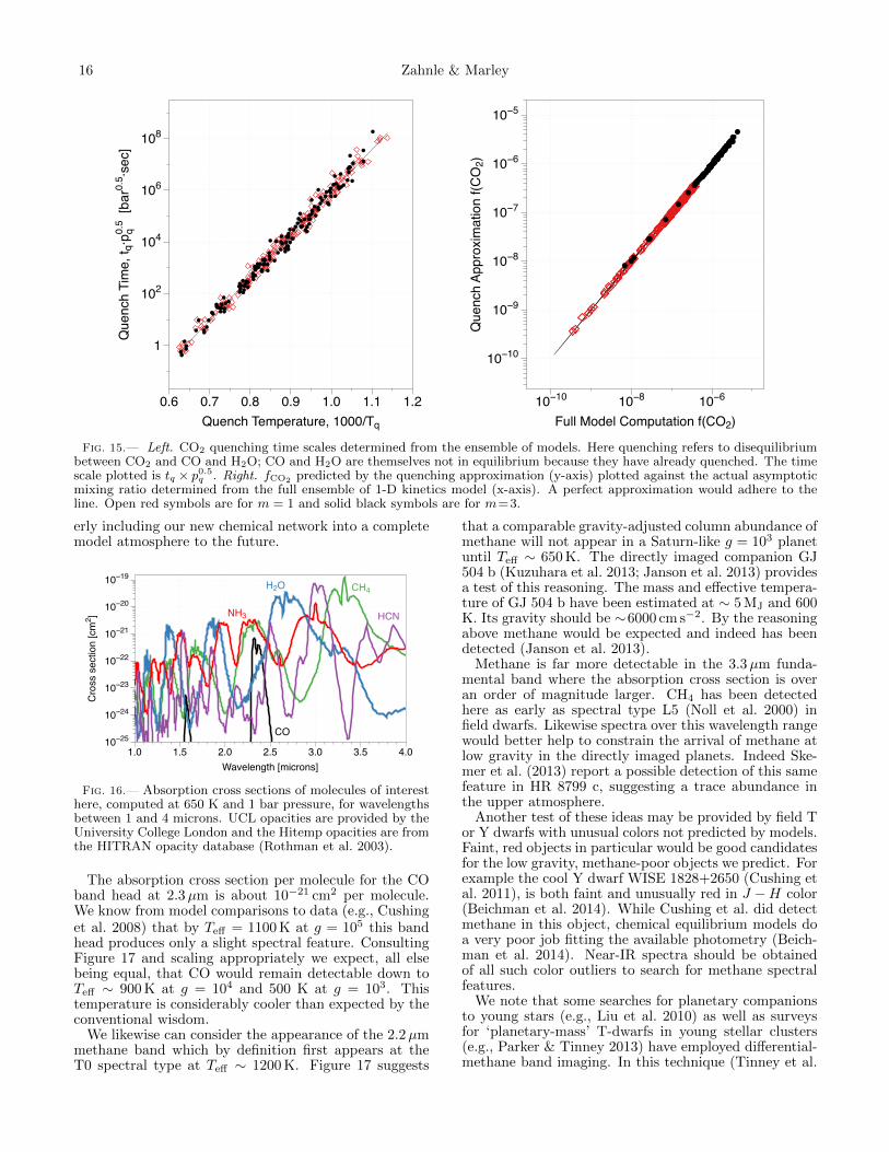
Fig. 15.— Left. CO2 quenching time scales determined from the ensemble of models. Here quenching refers to disequilibriumbetween CO2 and CO and H2O; CO and H2O are themselves not in equilibrium because they have already quenched. The timescale plotted is tq × p0.5

q . Right. fCO2 predicted by the quenching approximation (y-axis) plotted against the actual asymptoticmixing ratio determined from the full ensemble of 1-D kinetics model (x-axis). A perfect approximation would adhere to theline. Open red symbols are for m = 1 and solid black symbols are for m=3.

erly including our new chemical network into a completemodel atmosphere to the future.

CH4H2O

NH3 HCN

CO

Cro

ss s

ectio

n [c

m2 ]

10−25

10−24

10−23

10−22

10−21

10−20

10−19

Wavelength [microns]1.0 1.5 2.0 2.5 3.0 3.5 4.0

Fig. 16.— Absorption cross sections of molecules of interesthere, computed at 650 K and 1 bar pressure, for wavelengthsbetween 1 and 4 microns. UCL opacities are provided by theUniversity College London and the Hitemp opacities are fromthe HITRAN opacity database (Rothman et al. 2003).

The absorption cross section per molecule for the COband head at 2.3µm is about 10−21 cm2 per molecule.We know from model comparisons to data (e.g., Cushinget al. 2008) that by Teff = 1100 K at g = 105 this bandhead produces only a slight spectral feature. ConsultingFigure 17 and scaling appropriately we expect, all elsebeing equal, that CO would remain detectable down toTeff ∼ 900 K at g = 104 and 500 K at g = 103. Thistemperature is considerably cooler than expected by theconventional wisdom.

We likewise can consider the appearance of the 2.2µmmethane band which by definition first appears at theT0 spectral type at Teff ∼ 1200 K. Figure 17 suggests

that a comparable gravity-adjusted column abundance ofmethane will not appear in a Saturn-like g = 103 planetuntil Teff ∼ 650 K. The directly imaged companion GJ504 b (Kuzuhara et al. 2013; Janson et al. 2013) providesa test of this reasoning. The mass and effective tempera-ture of GJ 504 b have been estimated at ∼ 5 MJ and 600K. Its gravity should be ∼6000 cm s−2. By the reasoningabove methane would be expected and indeed has beendetected (Janson et al. 2013).

Methane is far more detectable in the 3.3µm funda-mental band where the absorption cross section is overan order of magnitude larger. CH4 has been detectedhere as early as spectral type L5 (Noll et al. 2000) infield dwarfs. Likewise spectra over this wavelength rangewould better help to constrain the arrival of methane atlow gravity in the directly imaged planets. Indeed Ske-mer et al. (2013) report a possible detection of this samefeature in HR 8799 c, suggesting a trace abundance inthe upper atmosphere.

Another test of these ideas may be provided by field Tor Y dwarfs with unusual colors not predicted by models.Faint, red objects in particular would be good candidatesfor the low gravity, methane-poor objects we predict. Forexample the cool Y dwarf WISE 1828+2650 (Cushing etal. 2011), is both faint and unusually red in J −H color(Beichman et al. 2014). While Cushing et al. did detectmethane in this object, chemical equilibrium models doa very poor job fitting the available photometry (Beich-man et al. 2014). Near-IR spectra should be obtainedof all such color outliers to search for methane spectralfeatures.

We note that some searches for planetary companionsto young stars (e.g., Liu et al. 2010) as well as surveysfor ‘planetary-mass’ T-dwarfs in young stellar clusters(e.g., Parker & Tinney 2013) have employed differential-methane band imaging. In this technique (Tinney et al.

Planetary Disequilibrium Chemistry 17

CO2

CH4

COC

olum

n D

ensi

ty [c

m-2

]

1018

1020

Teff

500 600 700 900 1100

N2

NH3

HCNCol

umn

Den

sity

[cm

-2]

1017

1018

1019

1020

Teff

500 600 700 900 1100

Fig. 17.— A sequence of models that illustrates how column densities of important carbon-bearing species change withtemperature Teff and gravity g. Kzz is restricted to 1013/g for CO, CH4, CO2, HCN. All Kzz are plotted for N2 and NH3.Columns are integrated above p = 10−5 ·g bars. Small symbols represent g= 1000, mid-sized symbols g=104, and big symbolsg= 105. Left. CO (black circles), CH4 (green diamonds), CO2 (blue squares). Right. N2 (blue diamonds), NH3 (red circles),HCN (gold squares).

2005) two images of a target are taken, one in a filter thatmatches the 1.7 − µm CH4 band and one which probesthe entire H band. When the two images are differenced,methane-bearing objects stand out as they are dark inthe CH4 filter. Our conclusions here suggest that suchtechniques must be used with caution as methane maysimply not yet be present in planetary-mass objects evenat effective temperatures below 1000 K.

Similar arguments can be made for the appearance ofother spectral features of interest. We expect that NH3

will appear at effective temperatures about 200 K coolerin planets compared to field brown dwarfs. HCN, with across section of 10−20 cm2 per molecule at 1.55µm is un-likely to be detectable in most objects as the computedcolumn abundances are less than 1018 cm−2. HCN’sprospects are poor at 3.0 microns despite a high cross-section unless the C/O ratio is higher than solar andwater’s abundance reduced. Water’s cross section is100-fold smaller, but with solar abundances its column(1−2×1021 cm−2) is 1000 times what HCN can reach atits best. Carbon dioxide has an absorption cross section10−17 cm2 per molecule at 4.2µm, and with abundancesapproaching 1018 cm−2 we expect it to be detectable ataround 900 to 1100 K in field brown dwarfs. Indeed theAKARI space telescope discovered CO2 features in sev-eral late L and early T dwarfs (Yamamura et al. 2010).Judging by Figure 17, we would predict CO2 to be de-tectable to 500 K and cooler in the lowest mass planets.

8. CONCLUSIONS

We use a reasonably complete 1-D chemical kineticscode to survey the parameter space that encompasses at-mospheres of cool brown dwarfs and warm young extra-solar giant planets. Our model contains only gas phasechemistry of small molecules containing H, C, N, O, andS. We use realistic p-T profiles for cloudless atmosphereswith effective temperatures between 500 and 1100 K andsurface gravities between 103 cm/s2 to 105 cm/s2. Verti-

cal transport is described by an eddy diffusivity Kzz thatwe vary over a wide range. Our objective is to describecarbon and nitrogen speciation, especially at lower (plan-etary) surface gravities. Overviews of what we found arepresented in Figure 4 for carbon and Figure 10 for nitro-gen.

We find that carbon in cloudless brown dwarfs is pre-dominantly in the form of methane at 900 K for g = 105

cm/s2. The small surface gravity of planets strongly dis-criminates against CH4 when compared to an otherwisecomparable brown dwarf. If vertical mixing is compara-ble to Jupiter’s, methane first predominates over CO inplanets cooler than 500 K. Sluggish vertical mixing canraise the transition to 600 K; clouds or more vigorousvertical mixing could lower it to 400 K.

The detectability of specific molecular features in aspectrum depends on the strength of the molecular ab-sorption cross sections as well as the gaseous abundance.Nevertheless a natural prediction of our model is thatthere will be cool planets with no methane observedin the H or K spectral bands. The refractory behav-ior of CO in low gravity objects is likely at least par-tially responsible for the lack of cool planets found bythe NICI survey, which relied upon the methane absorp-tion H band to identify planets (Liu et al. 2010).

Ammonia is also sensitive to gravity, but unlikemethane and CO, ammonia is insensitive to mixing,which makes it a proxy for gravity. We did not ex-plore temperatures low enough to determine the tran-sition from N2 to ammonia in planets, but it is nearlyas abundant as N2 at 500 K in brown dwarfs, which isbroadly consistent with the observed properties of theY dwarfs (Cushing et al. 2011) for which NH3 is seenin H band. On the other hand, ammonia persists as anabundant minor species to rather high temperatures andthis is consistent with it being readily detected in mid-IRspectra of T-dwarfs (Cushing et al. 2006). HCN might

18 Zahnle & Marley

become interesting in high gravity brown dwarfs if verti-cal mixing is very vigorous.

When expressed in terms of quenching parameters,nearly all our results for CO and CH4 can be reducedto a simple equation in Arrhenius form that is easy touse but not easy to interpret. From a strictly practicalperspective, what we find is close to what one gets us-ing Prinn and Barshay (1977)’s algorithm in its originalform (a fortuitous accident of using too high a rate forthe wrong reaction). The apparent simplicity is some-what surprising given the complexity of the chemistryinvolved and the many different ways the system hasbeen described in the literature. Nor is our result quitewhat we expected. First, we find that the timescale tCO

for hydrogenation of CO is shorter for higher metallic-ity. Because the forward reactions that destroy CO haveno metallicity dependence, we infer that metallicity de-pendence enters through the reverse reaction (oxidationof CH4). By definition the reverse reaction is as fast asthe forward reaction while in equilibrium, but it falls offmore quickly than the forward reaction as the tempera-ture drops. The important forward reactions are linearin metallicity whilst the important reverse reactions arequadratic in metallicity.

Second, we find that tCO is inversely proportional topressure. Analyses based on isolating a limiting reactionpredict a stronger dependence on pressure, typically p−2.The weaker p−1 pressure dependence is expected for areaction involving CO itself, such as

H2 + CO→ HCO + H. (45)

It is interesting that R45 actually does have the highest∆G value in the CO hydrogenation sequence, and there-fore the highest energy barrier, and that the magnitudeof ∆G of R45 is what we infer in Eq 14. But it is alsoquite clear from Figure 7 that equilibrium breaks downbetween CH3OH and CH4 well before if breaks down be-tween CO and CH3OH, as was found by Moses et al.(2011). Reactions involving CH3OH imply a p−2 pres-sure dependence, because the equilibrium abundance ofCH3OH with respect to CO goes as the square of the H2

pressure. The system behaves—both in the 40,000 K en-ergy barrier and the p−1 pressure dependence— as if theoverall rate depends on the entry reaction R45 ratherthan on the rate of R23 in which equilibrium actuallybreaks down. The apparent paradoxes might be resolvedthrough a more complete analysis of the reverse reac-tions, or they may result from systematic biases stem-ming from our treating the mixing length as equal to ascale height, rather than as the complex function of manyvariables that it probably is (Smith 1998).

For nitrogen and ammonia we were unable to recoveran emergent Arrhenius-like behavior from the full sys-tem. On the other hand, it was easy to devise a goodquench approximation, and we also found that some pub-lished quench approximations (e.g., Fegley and Lodders1994) work very well. For HCN, we met with mixed

success. We did find emergent Arrhenius-like behav-iors, and we developed a new quench approximation thatworks quite well for our models. On the other handthere does not yet appear to be a consensus on whatthe quench chemistry of HCN actually is. We found awide scatter of different outcomes when comparing dif-ferent published quench schemes. We think our quenchapproximation should work well for warm objects whereHCN is predicted to be relatively abundant but, becausewe did not consider hypothetical hydrogenation channelsthrough methylamine (Moses et al. 2010), our modelsmay overestimate fHCN, especially in cooler objects.

There are many effects that our models do not address.None of these effects have much sway over our quenchapproximations, but they have much to do with whatmight actually be present in a real atmosphere.

Clouds are likely the most important. Adding infraredopacity to an atmosphere is effectively equivalent to re-ducing the gravity. This is because opacity raises the p-Tprofile (i.e., the adiabat) to a lower pressure for a giveneffective temperature. A cloudy atmosphere favors COand N2 over CH4 and NH3, other things equal. Increas-ing metallicity also increases opacity to the detriment ofmethane and ammonia.

Another issue for real worlds is that Kzz may be muchsmaller in higher altitude radiative regions of the atmo-sphere than it is in the convecting region. The radiativestratosphere is the part of the atmosphere where Kzz

the modeling parameter is most suspect. For N2 andNH3 pronounced vertical structure in Kzz will not mat-ter much. For CO and CH4, sharply lower values of Kzz

in the stratosphere might be important, because if Kzz

is low enough, the atmosphere can have a second quenchpoint in the stratosphere. Such behavior no problem to afull kinetics model, but it can make implementing quenchapproximations more complicated.

Photochemistry induced by irradiation from a nearbystar can deplete NH3 and increase CO2 and HCN. Light-ning and/or impact shocks in cool NH3- and CH4-richatmospheres can generate CO and HCN (Chameides andWalker 1981). In warmer objects, catalysts that may bepresent in metallic clouds (here we mean real metals) willlower the quench point and thus will favor NH3, CH4, andCO4 (Prinn and Fegley 1987).

All of these ideas will be put to the test by the directlyimaged planets that are expected to be discovered in thecoming months and years. Constraining the composi-tion of their atmospheres will no doubt be a rewardingendeavour.

ACKNOWLEDGMENTS

The authors thank Richard Freedman, Caroline Mor-ley, Julianne Moses, Didier Saumon, and Channon Viss-cher for many insightful discussions and occasional coursecorrections. The authors thank the NASA Planetary At-mospheres Program for support of this work.

REFERENCES

Abelson, P. (1966). Chemical events on the primitive Earth. Proc.Natl. Acad. Sci. USA 55, 1365-1372.

Barman, T., Macintosh, B., Konopacky, Q.M., Marois, C. (2011).Clouds and Chemistry in the Atmosphere of Extrasolar PlanetHR8799b. Astrophys. J. 733, article id. 65, 18 pp.

Planetary Disequilibrium Chemistry 19

Barman, T., Macintosh, B., Konopacky, Q.M., Marois, C. (2011).The Young Planet-mass Object 2M1207b: A Cool, Cloudy, andMethane-poor Atmosphere. Astrophys. J. Lett. 735, article id.L39, 5 pp.

Beichman, C., Gelino, C. R., Kirkpatrick, J. D., et al. 2014,Astrophys. J. 783, 68

Bezard, B., Lellouch, E., Strobel, D., Maillard, J.-P., Drossart, P.(2002). Carbon Monoxide on Jupiter: Evidence for BothInternal and External Sources. Icarus 159, 95-111.

Burcat, A., Ruscic, B. 2005, Third Millennium Ideal Gas andCondensed Phase Thermochemical Database for Combustionwith Updates from Active Thermochemical Tables. ReportANL 05-20 and TAE 960.

Burningham et al 2011, MNRAS 414, 3590.Burrows, A., Marley, M., Hubbard, W. B., et al. 1997, ApJ, 491,

856Chameides, W., Walker, J.C.G., Nagy, A.F. (1979). Possible

chemical impact of planetary lightning in the atmospheres ofVenus and Mas. Nature 280, 820-822.

Chameides, W., Walker, J.C.G. (1981). Rates of fixation bylightning of carbon and nitrogen in possible primitiveatmospheres. Origins of Life 11, 291-302.

Cooper, C.S., Showman, A.P. (2006). Dynamics andDisequilibrium Carbon Chemistry in Hot Jupiter Atmospheres,with Application to HD 209458b. Astrophys. J. 649, 1048-1063.

Cushing, M. C., Roellig, T. L., Marley, M. S., et al. 2006,Astrophys. J. 648, 614

Cushing, M. C., Marley, M. S., Saumon, D., et al. 2008,Astrophys. J. 678, 1372

Cushing, M. C., Kirkpatrick, J. D., Gelino, C. R., et al. 2011,ApJ, 743, 50

Fegley, B.J., Lodders, K. (1994). Chemical models of the deepatmospheres of Jupiter and Saturn. Icarus 110, 117-154.

Fegley, B.J., Lodders, K. (1996). Atmospheric Chemistry of theBrown Dwarf Gliese 229B: Thermochemical EquilibriumPredictions. Astrophys. J. Lett. 472, p.L37.

Freytag et al (2010). Astron. Astrophys. 513, 19.Geballe, T. R., Saumon, D., Golimowski, D. A., et al. 2009,

Astrophy. J. 695, 844Gierasch, P. J., & Conrath, B. J. 1985, Recent Advances in

Planetary Meteorology, 121Haworth, N.L., Mackie, J.C., Bacskay, G.B. (2003). An Ab Initio

Quantum Chemical and Kinetic Study of the NNH + OReaction Potential Energy Surface: How Important Is ThisRoute to NO in Combustion? J. Phys. Chem. A 107, 6792 -6803.

Hubeny, I., Burrows, A. (2007). A systematic study of departuresfrom chemical equilibrium in the atmospheres of substellarmass objects. Astrophy. J. 669, 1248-1261.

Janson, M., Brandt, T. D., Kuzuhara, M., et al. 2013, Astrophys.J. Let., 778, L4

Jasper, A.W., Klippenstein, S.J., Harding, L.B. (2007). Secondarykinetics of methanol decomposition. J. Phys. Chem. A 111,8699-8707.

Kirkpatrick, J. D. 2005, Ann. Rev. Astron. Astrophys. 43, 195Kirkpatrick, J. D., Gelino, C. R., Cushing, M. C., et al. 2012,

ApJ, 753, 156Konopacky, Q. M., Barman, T. S., Macintosh, B. A., & Marois,

C. 2013, Science, 339, 1398Kuzuhara, M., Tamura, M., Kudo, T., et al. 2013, Astrophys. J.

774, 11Liang, M.C., Parkinson, C.D., Lee, A.Y.-T., Yung, Y.L., Seager,

S. (2003). Source of atomic hydrogen in the atmosphere of HD209458b. Astrophys. J. 596, L247?L250.

Line, M.R., Liang, M.-C., Yung, Y.L. (2010). High-TemperaturePhotochemistry in the Atmosphere of HD 189733b. Astrophys.J. 717, 496-502.

Line, M.R., Vasisht, G., Chen, P., Angerhausen, D., Yung, Y.L.(2011). Thermochemical and Photochemical Kinetics in CoolerHydrogen-dominated Extrasolar Planets: A Methane-poorGJ436b? Astrophys. J. 738, article id. 32, 14 pp.

Liu, M. C., Wahhaj, Z., Biller, B. A., et al. 2010, Proc. SPIE,7736,

Lodders, K. (2004). Revised and updated thermochemicalproperties of the gases mercapto HS, disulfur monoxide S2O,thiazyl NS, and thioxophosphino PS. J. Phys. Chem. Ref. Data33, 357-367.

Lodders, K., Fegley, B.J. (2002). Atmospheric Chemistry in GiantPlanets, Brown Dwarfs, and Low-Mass Dwarf Stars. I. Carbon,Nitrogen, and Oxygen. Icarus 155, 393-424.

Marley, M.S., Fortney, J.J., Seager, S., Barman, T. (2007). AnImposing and Comprehensive Title. In Protostars and PlanetsV. Eds. B. Reipurth, D. Jewitt, and K. Keil. Univ. Ariz. Press,Tucson, pp. 733–747.

Matus, M.H., Arduengo, A.J., Dixon, D.A. (2006). The heats offormation of diazene, hydrazine, N2H3+, N2H5+, N2H, andN2H3 and the Methyl Derivatives CH3NNH, CH3NNCH3, andCH3HNNHCH3. J Phys Chem A. 110, 10116-10121.

Miller-Ricci Kempton, E., Zahnle, K., Fortney, J.J. (2011). TheAtmospheric Chemistry of GJ 1214b: Photochemistry andClouds. Astrophys. J. 745, 3 (13pp).

Morley, C.V., Fortney, J.J., Kempton, E.M.R., Marley, M.S.,Visscher, C., Zahnle, K.J. (2013). Quantitatively Assessing theRole of Clouds in the Transmission Spectrum of GJ 1214b.Astrophys. J. 775, article id. 33, 13 pp.

Moses, J.I., Visscher, C., Keane, T.C., Sperierd, A. (2010). Onthe abundance of non-cometary HCN on Jupiter. FaradayDiscuss., 2010, 147, 103-136.

Moses, J.I., Visscher, C., Fortney, J.J., Showman, A.P., Lewis,N.K., Griffith, C.A., Klippenstein, S.J., Shabram, M., Friedson,A.J., Marley, M.S., Freedman, R.S. (2011). DisequilibriumCarbon, Oxygen, and Nitrogen Chemistry in the Atmospheresof HD 189733b and HD 209458b. Astrophys. J. 737, article id.15, 37 pp.

Moses, J.I., Madhusudhan, N., Visscher, C., Freedman, R.S.(2013). Chemical Consequences of the C/O Ratio on HotJupiters: Examples from WASP-12b, CoRoT-2b, XO-1b, andHD 189733b. Astrophys. J. 763, article id. 25, 26 pp.

Moses, J.I., Line, M.R., Visscher, C., Richardson, M.R.,Nettelmann, N., Fortney, J.J., Barman, T.S., Stevenson, K.B.,Madhusudhan, N. (2013). Compositional Diversity in theAtmospheres of Hot Neptunes, with Application to GJ 436b.Astrophys. J. 777, article id. 34, 23 pp.

Moses, J.I. (2014). Chemical Kinetics on Extrasolar Planets. Phil.Trans. Roy. Soc. A. Fate Unknown.

Noll, K. S., Geballe, T. R., & Marley, M. S. 1997, Astrophys. J.Lett. 489, L87

Noll, K. S., Geballe, T. R., Leggett, S. K., & Marley, M. S. 2000,Astrophys. J. Lett. 541, L75

Odd nitrogen production by meteoroids. J. Geophys. Res. 83,4029-4035.

Parker, S. R., & Tinney, C. G. 2013, MNRAS, 430, 1208Prinn, R.G., Barshay, S.S. (1977). Carbon monoxide on Jupiter

and implications for atmospheric convection. Science 198,1031-1034.

Prinn, R.G., Fegley, B. (1981). Kinetic inhibition of CO and N2

reduction in circumplanetary nebulae: Implications for satellitecomposition. Astrophys. J. 249, 308-317.

Prinn, R.G., Fegley, B. (1987). Solar nebula Chemistry: origin ofplanetary, satellite, and planetary volatiles. In Origin andEvolution of Planetary and Satellite Atmospheres. Eds. AtreyaSK, Pollack JB, Matthews MS, Univ of Arizona Press, pp78-136.

Rauk ,A., Boyd, R.J., Boyd, S.L., Henry, D.J., Radom, L. (2003).Alkoxy radicals in the gaseous phase: beta-scission reactionsand formation by radical addition to carbonyl compounds.Can. J. Chem. 81, 431-442.

Rothman, L.S., et al. 2003, J. Quant. Spect. & Rad. Tran. 111,2139.

Saumon, D., Geballe, T. R., Leggett, S. K., et al. 2000,Astrophys. J. 541, 374

Saumon, D., Marley, M. S., Cushing, M. C., et al. 2006,Astrophys. J. 647, 552

Saumon, D., & Marley, M. S. 2008, Astrophys. J. 689, 1327Skemer, A. J., Marley, M. S., Hinz, P. M., et al. 2014, Astrophys.

J., in press, arXiv:1311.2085Smith, M.D. (1998). Estimation of a length scale to use with the

quench level approximation for obtaining chemical abundances.Icarus 132, 176-184.

Tinney, C. G., Burgasser, A. J., Kirkpatrick, J. D., & McElwain,M. W. 2005, Astron. J., 130, 2326

Visscher, C.W., Moses, J.I., Saslow, S.A. (2010). The deep waterabundance on Jupiter: New constraints from thermochemicalkinetics and diffusion modeling. Icarus 209, 602-615.

20 Zahnle & Marley

Visscher, C.W., Moses, J.I. (2011). Quenching of carbon monoxideand methane in the atmospheres of cool brown dwarfs and hotJupiters. Astrophys. J. 738, article id. 72, 12 pp.

Visscher, C.W. (2012). Chemical timescales in the atmospheres ofhighly eccentric exoplanets. Astrophys. J. 757, article id. 5, 8pp.

Vuitton, V., Yelle, R.V., Lavvas, P., Klippenstein, S.J. (2012).Rapid association reactions at low pressure: impact on theformation of hydrocarbons on Titan. Astrophys. J. 744, articleid. 11, 7 pp.

Yamamura, I., Tsuji, T., & Tanabe, T. 2010, Astrophys. J. 722,682

Yung, Y.L., Drew, W.A., Pinto, J.P., Friedl, R.R. (1988).Estimation of the reaction rate for the formation of CH3O fromH + H2CO: Implications for chemistry in the Solar System.Icarus 73, 516-526.

Zahnle, K.J., Claire, M.W., Catling, D.C. (2006). The loss ofmass-independent fractionation in sulfur due to aPaleoproterozoic collapse of atmospheric methane. Geobiology4, 271-282.

Zahnle, K.J., Haberle, R.M., Catling, D.C., Kasting, J.F. (2008).Mars Photochemistry Paper. J. Geophys. Res. 113, E11004,doi:10.1029/2008JE003160.

Zahnle, K.J., Marley, M.S., Freedman, R.S., Lodders, K., Fortney,J.J. (2009). Atmospheric sulfur chemistry on hot Jupiters.”Astrophys. J. Lett. 701, L20-L24.

Zel’dovich, Ya.B., Raizer, Ya. (1967) Physics of Shock Waves andHigh Temperature Phenomena, Vol. 2, pp. 566?571, AcademicPress, NY.