Embed Size (px)
Citation preview

Keith C.C. Chan
Department of Computing
The Hong Kong Polytechnic University
Ch 2 Discovering Association Rules
COMP 578Data Warehousing & Data Mining

2
The AR Mining Problem
Given a database of transactions. Each transaction being a list of items. E.g. purchased by a customer in a visit.
Find all rules that correlate the presence of one set of items with that of another set of items E.g., 30% of people who buys diapers also
buys beer.

3
Motivation & Applications (1)
If we can find such associations, we will be able to answer: ??? beer (What should the company do to boost beer sales?) Diapers ??? (What other products should the store stocks up?) Attached mailing in direct marketing.

4
Originally for marketing to understand purchasing trends. What products or services customers tend to purchase at
the same time, or later on? Use market basket analysis to plan:
Coupon and discounting: Do not offer simultaneous discounts on beer and diapers if they
tend to be bought together. Discount one to pull in sales of the other.
Product placement. Place products that have a strong purchasing relationship close
together. Place such products far apart to increase traffic past other items.
Motivation & Applications (2)
5
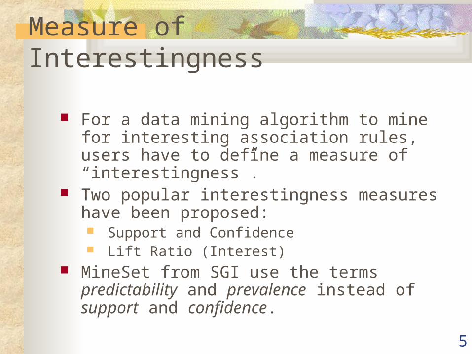
Measure of Interestingness
For a data mining algorithm to mine for interesting association rules, users have to define a measure of “interestingness”.
Two popular interestingness measures have been proposed: Support and Confidence Lift Ratio (Interest)
MineSet from SGI use the terms predictability and prevalence instead of support and confidence.

6
Given rule X & Y => Z Support, S = P(X Y Z)
where A B indicates that a transaction contains both X and Y
(union of item sets X and Y)
[# of tuples containing both A & B / total # of tuples]
Confidence, C = P(Z | X Y ) P(Z | X Y ) is a conditional probability that a transaction having {XY} also contains Z
[# of tuples containing both X&Y&Z / # of tuples containing X&Y]
The Support and Confidence
7
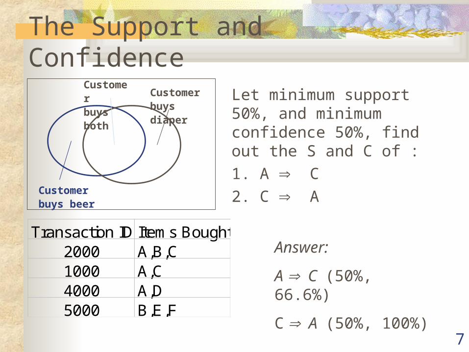
The Support and Confidence
Transaction ID Items Bought2000 A,B,C1000 A,C4000 A,D5000 B,E,F
Let minimum support 50%, and minimum confidence 50%, find out the S and C of :
1. A C
2. C A
Customerbuys diaper
Customerbuys both
Customerbuys beer
Answer:
A C (50%, 66.6%)
C A (50%, 100%)

8
How Good is a Predictive Model? Response curves- How does the response rate of a targeted selection compare to a random selection?

9
What is A Lift Ratio? (1)
Consider the rule: When people buy diapers they also buy beer 50 percent
of the time.
It states an explicit percentage (50% of the time). Consider this other rule:
People who purchase a VCR are three times more likely to also purchase a camcorder.
The rule used the comparative phrase “three times more likely”?

10
The probability is compared to the baseline likelihood.
The baseline likelihood is the probability of the event occurring independently. E.g., if people normally buy beer 5% of the time,
then the first rule could have said “10 times more likely.”
The ratio in this kind of comparison is called lift. A key goal of an association rule mining exercise
is to find rules that have the desired lift.
What is A Lift Ratio? (2)

11
Lift Ratio As Interestingness
X 1 1 1 1 0 0 0 0Y 1 1 0 0 0 0 0 0Z 0 1 1 1 1 1 1 1
Rule Support ConfidenceX=>Y 25% 50%X=>Z 37.50% 75%
An Example:
Support and Confidence of X=>Z dominates
X and Y, positively correlated,
X and Z, negatively related

12
Lift Ratio As Interestingness It is a measure of dependent or correlated events
The lift of rule X => Y
Lift = 1 means X and Y are independent events
Lift < 1 means X and Y are negatively correlated
Lift > 1 means X and Y are positively correlated
(better than random)
)(
)|(, YP
XYPlift YX
)()(
)(
YPXP
YXPor
Apriori = P(Y)Confidence=P(Y|X)

13
AR Mining with Lift Ratio (1)
To understand what lift ratio is, consider the following: 500,000 transactions
20,000 transactions contain diapers (4 percent) 30,000 transactions contain beer (6 percent) 10,000 transactions contain both diapers and beer (2
percent) Confidence measures how much a particular item is
dependent on another. When people buy diapers, they also buy beer 50% of
the time (10,000/20,000). The confidence for this rule is 50%.

14
The inverse rule could be stated as: When people buy beer they also buy diapers 1/3 of
the time (Conf=33.33% = 10,000/30,000).
In the absence of any knowledge about what else was bought, the following can be computed:
People buy diapers 4 percent of the time. People buy beer 6 percent of the time.
4% and 6% are called the expected confidence (or baseline likelihood, or A Priori Probability) of buying diapers or beer.
AR Mining with Lift Ratio (2)

15
Lift measures the difference between the confidence of a rule and the expected confidence.
Lift is one measure of the strength of an effect. If people who bought diapers also bought beer
8% of the time, then the effect is small if expected confidence is 6%.
If the confidence is 50%, and lift is more than 8 times (when measured as a ratio), then the interactions between diapers and beer is very strong.
AR Mining with Lift Ratio (3)

16
Consider item sets with three items: 10,000 transactions contain wipes. 8,000 transactions contain wipes and diapers (80%). 220 transactions contain wipes and beer (2.2%). 200 transactions contain wipes, diapers and beer
(2%). The complete set of 12 rules is presented in a table
along with their confidence, support and lift.
AR Mining with Lift Ratio : An Example

17
LHS RHS Exp Conf (%)
Conf (%)
Lift Ratio
Supp (%)
1 Diapers Beer 6.00 50.00 8.33 2.00 2 Beer Diapers 4.00 33.33 8.33 2.00 3 Diapers Wipes 2.00 40.00 20.00 1.60 4 Wipes Diapers 4.00 80.00 20.00 1.60 5 Wipes Beer 6.00 2.20 0.37 0.04 6 Beer Wipes 2.00 0.73 0.37 0.04 7 Diapers
& Wipes Beer 6.00 2.50 0.42 0.04
8 Diapers & Beer
Wipes 2.00 2.00 1.00 0.04
9 Beer & Wipes
Diapers 4.00 90.91 22.73 0.04
10 Diapers Wipes & Beer
0.044 1.00 22.73 0.04
11 Wipes Diapers & Beer
2.00 2.00 1.00 0.04
12 Beer Diapers & Wipes
1.60 0.67 0.42 0.04
AR Mining with Lift Ratio : An Example

18
The greatest amount of lift, if measured as a ratio, is found in the 9th and 10th rules.
Both have a lift greater than 22, computed as 90.91/4 and 1/0.044.
For the 9th rule, the lift of 22 means: People who purchase wipes and beer are 22 times more
likely to also purchase diapers than people who do not. Note the negative lift (lift ratio less than 1) in the
5th, 6th, 7th and last rules. The latter two rules both have a lift ratio of
approximately 0.42.
AR Mining with Lift Ratio : An Example

19
Negative lift on the 7th rule means that people who buy diapers and wipes are less likely to buy beer than one would expect.
Rules with very high or very low confidence model an anomaly. If a rule says, with a confidence of 1 (100%), that
whenever people bought pet food they also bought pet supplies.
Further investigation show that was for one day only. There was a special giveaway.
AR Mining with Lift Ratio : An Example
20
Most rules have dairy on the right hand side. Milk or eggs are so commonly purchased, “dairy”
is quite likely to show up in many rules. Ability to exclude specific items is very useful. Interesting rules are:
Have a very high or very low lift. Do not involve items that appear on most transactions. Have support that exceeds a threshold.
Low support might simply be due to a statistical anomaly. Rules that are more general are frequently desirable. Sometimes interesting to differentiate between diapers sold in
boxes vs. diapers sold in bulk.
AR Mining with Lift Ratio : An Example

21
Lift Ratio and Sample Size
Consider the association A => B. A lift ratio can be very large even if the
number of transactions having A and B together or separately are very small.
To take sample size into consideration, one can consider using the support and confidence as interestingness measures.

22
Complexity of AR Mining Algorithms
An association algorithm is simply a counting algorithm.
Probabilities are computed by taking ratios among various counts.
If item hierarchies are in use, then some translation (or lookup) is needed.
One must carefully control the sizes of the item sets because of combinatorial explosion problem.
23
Large grocery stores stock sell more than 100,000 different items.
There can be 5 billion possible item pairs, and 1.7 x 10¹⁴ sets of three items.
An item hierarchy can be used to reduce this number to a manageable size.
There is unlikely to be a specific relationship between Pampers in the 30-count box and Blue Ribbon in 12oz cans.
Complexity of AR Mining Algorithms

24
If there is such a relationship, it is probably subsumed by the more general relationship between diapers and beer.
Using an item hierarchy reduces the number of combinations.
It also helps to find more general higher-level relationships such as those between any kind of diapers and any kind of beer.
Complexity of AR Mining Algorithms

25
The combinatorial explosion problem: Even if you use an item hierarchy to group items together so
that the average group size is 50. Reducing 100,000 items to 2,000 item groups. With 2,000 item groups there are still almost 2 million paired
item sets. An algorithm might require up to 2 million counting registers. There are 1.3 billion three-item item sets! Many combinations will never occur. Some sort of dynamic memory or counter allocation and
addressing scheme will be needed.
Complexity of AR Mining Algorithms

26
The Apriori Algorithm
For rule A C:support = support({A ^ C}) = 50%
confidence = support({A ^ C})/support({A}) = 66.6%
The Apriori principle:Any subset of a frequent itemset must be frequent
Transaction ID Items Bought2000 A,B,C1000 A,C4000 A,D5000 B,E,F
Frequent Itemset Support{A} 75%{B} 50%{C} 50%{A,C} 50%
Min. support 50%Min. confidence 50%

27
Applying Apriori Algorithm
TID Items100 1 3 4200 2 3 5300 1 2 3 5400 2 5
Database D itemset sup.{1} 2{2} 3{3} 3{4} 1{5} 3
itemset sup.{1} 2{2} 3{3} 3{5} 3
Scan D
C1L1
itemset{1 2}{1 3}{1 5}{2 3}{2 5}{3 5}
itemset sup{1 2} 1{1 3} 2{1 5} 1{2 3} 2{2 5} 3{3 5} 2
itemset sup{1 3} 2{2 3} 2{2 5} 3{3 5} 2
L2
C2 C2
Scan D
C3 L3itemset{2 3 5}
Scan D itemset sup{2 3 5} 2
ANIMATEDDEMO

28
Improving Apriori’s Efficiency Hash-based itemset counting: A k-itemset whose corresponding hashing
bucket count is below the threshold cannot be frequent
Transaction reduction: A transaction that does not contain any frequent
k-itemset is useless in subsequent scans
Partitioning: Any itemset that is potentially frequent in DB must be
frequent in at least one of the partitions of DB
Sampling: mining on a subset of given data, lower support threshold + a
method to determine the completeness
Dynamic itemset counting: add new candidate itemsets only when all of
their subsets are estimated to be frequent.

29
Is Apriori Fast Enough? The core of the Apriori algorithm:
Use frequent (k – 1)-itemsets to generate candidate frequent k-itemsets
Use database scan and pattern matching to collect counts for the candidate itemsets
The bottleneck of Apriori: candidate generation Huge candidate sets:
104 frequent 1-itemset will generate 107 candidate 2-itemsets To discover a frequent pattern of size 100, e.g., {a1, a2, …, a100},
one needs to generate 2100 1030 candidates.
Multiple scans of database: Needs (n +1 ) scans, n is the length of the longest pattern

30
Multiple-Level ARs Items often form hierarchy. Items at the lower level are expected to have
lower support. Rules regarding itemsets at appropriate levels could be quite useful. Transaction database can be encoded based on
dimensions and levels It is smart to explore shared multi-level mining
(Han & Fu,VLDB’95).

31
Mining Multi-Level Association A top_down, progressive deepening approach:
First find high-level strong rules: milk bread [20%, 60%].
Then find their lower-level “weaker” rules: 2% milk wheat bread [6%, 50%].
Variations at mining multiple-level association rules. Level-crossed association rules:
2% milk Wonder wheat bread Association rules with multiple, alternative hierarchies:
2% milk Wonder breadg

32
Multi-level Association: Uniform Support vs. Reduced Support (1)
Uniform Support: the same minimum support for all levels + One minimum support threshold. No need to examine
itemsets containing any item whose ancestors do not have minimum support.
– Lower level items do not occur as frequently. If support threshold
too high miss low level associations. too low generate too many high level associations.
33
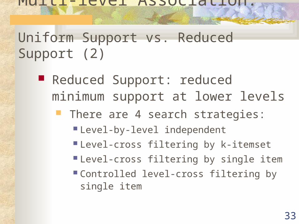
Reduced Support: reduced minimum support at lower levels There are 4 search strategies:
Level-by-level independent Level-cross filtering by k-itemset Level-cross filtering by single item Controlled level-cross filtering by single item
Multi-level Association: Uniform Support vs. Reduced Support (2)

34
Uniform SupportMulti-level mining with uniform support
Milk
[support = 10%]
2% Milk
[support = 6%]
Skim Milk
[support = 4%]
Level 1min_sup = 5%
Level 2min_sup = 5%

35
Reduced SupportMulti-level mining with reduced support
2% Milk
[support = 6%]
Skim Milk
[support = 4%]
Level 1min_sup = 5%
Level 2min_sup = 3%
Back
Milk
[support = 10%]

36
Multi-level Association:Redundancy Filtering
Some rules may be redundant due to “ancestor” relationships between items.
Example milk wheat bread, [support = 8%, confidence = 70%] 2% milk wheat bread, [support = 2%, confidence = 72%]
We say the first rule is an ancestor of the second rule.
A rule is redundant if its support is close to the “expected” value, based on the rule’s ancestor.

37
Multi-Level Mining: Progressive Deepening A top-down, progressive deepening approach:
First mine high-level frequent items: milk (15%), bread (10%)
Then mine their lower-level “weaker” frequent itemsets: 2% milk (5%), wheat bread (4%)
Different min_support threshold across multi-levels lead to different algorithms: If adopting the same min_support across multi-levels
then toss t if any of t’s ancestors is infrequent.
If adopting reduced min_support at lower levelsthen examine only those descendents whose ancestor’s support is
frequent/non-negligible.

38
AR Representation Scheme In words:
60% of people who buys diapers also buys beers and 0.5% buys both.
In first-order logic or PROLOG-like statement: buys(x, “diapers”) buys(x, “beers”) [0.5%, 60%]
Also representation as if-then rules. If diapers in Itemset THEN beers in Itemset [0.5%, 60%] If people buy diapers, they also buy beers 60% of the
time, 0.5% of the people buy both.

39
Presentation of Association Rules (Tabular )

40
Visualization of Association Rule Using Plane Graph

41
Visualization of Association Rule Using Rule Graph

42
Sequential Apriori Algorithm (1)
1. Sort Phase. This step implicitly converts the original transaction database into a database of sequences.
2. Litemset Phase. In this phase we find the set of all litemsets L. We are also simultaneously finding the set of all large 1-sequences.
3. Transformation Phase. We need to repeatedly determine which of a given set of large sequences are contained in a customer sequence. We transform each customer sequence into an alternative representation.
4. Sequence Phase. Use the set of litemsets to find the desired sequences. Algorithms for this phase below.
5. Maximal Phase. Find the maximal sequences among the set of large sequences. In some algorithms this phase is combined with the sequence phase to reduce the time wasted in counting non maximal sequences.
The problem of mining sequential patterns can be split into the following phases:
REFERENCE:Mining Sequential Patterns

43
Sequential Apriori Algorithm (2)
There are two families of algorithms- count-all and count-some. The count-all algorithms count all the large sequences, including non-maximal sequences. The non-maximal sequences must then be pruned out (in the maximal phase).
AprioriAll is a count-all algorithm, based on the Apriori algorithm for finding large itemsets.
Apriori-Some is a count-some algorithm. The intuition behind these algorithms is that since we are only interested in maximal sequences, we can avoid counting sequences which are contained in a longer sequence if we first count longer sequences.

44
AprioriAll Algorithm (1)
Step 1 Step 2
Step 3
Minimum support = 25%

45
AprioriAll Algorithm (2)Step 4
L1 = large 1-sequences; // Result of litemset phase
for ( k = 2; Lk-1 0; k++) do
begin Ck = New Candidates generated from Lk-1 (see next slide)
foreach customer-sequence c in the database do Increment the count of all candidates in Ck that are
contained in c. Lk = Candidates in Ck with minimum support.
end Answer = Maximal Sequences in k Lk ;

46
The apriori-generate function takes as argument Lk-1, the set of all large
(k-1)-sequences. It works as follows. First join Lk-1 with Lk-1
insert into Ck
select p.litemset1 , ..., p.litemsetk-1 , q.litemsetk-1
from Lk-1 p, Lk-1 q
where p.litemset1 = q.litemset1 , . . .,
p.litemsetk-2 = q.litemsetk-2 ;
Next delete all sequences c Ck such that some (k-1)-subsequence of c is
not in Lk-1
Apriori Candidate Generation
AprioriAll Algorithm (3)

47
REFERENCE:Sequential Hash Tree for fast accesshttp://www-users.cs.umn.edu/~mjoshi/hpdmtut/sld144.htm
Hash Tree used for fast search of candidate occurrences. Similar to association rule discovery, except for following differences.
• Every event-timestamp pair in the timeline is hashed at the root.
• Events eligible for hashing at the next level are determined by the maximum gap (xg), window size (ws), and span (ms) constraints.
Count Operation in Sequential Apriori

48
Exercises:
1. What is the difference between the algorithms of Apriori and AprioriAll?
2. What happens if min. support and confidence are set too low / high?
3. Give a short example to show that items in a strong association rule may actually be negatively correlated.

49
END OF CHAPTER 2
BACK TO MAIN