Embed Size (px)
Citation preview
SAFYR7
KAPPABRIDGE CONTROL SOFTWARE
User Manual
Version 1.1April 2018

Safyr7 – User Manual Contents
Contents
1 Introduction 1
2 Getting Started 32.1 System Requirements . . . . . . . . . . . . . . . . . . . . . . . . . . . . . . . . . 3
2.2 Program Installation . . . . . . . . . . . . . . . . . . . . . . . . . . . . . . . . . . 3
2.3 Program Execution . . . . . . . . . . . . . . . . . . . . . . . . . . . . . . . . . . . 5
2.4 Instrument Activation . . . . . . . . . . . . . . . . . . . . . . . . . . . . . . . . . 6
2.4.1 Generic Steps . . . . . . . . . . . . . . . . . . . . . . . . . . . . . . . . . . 6
2.4.2 Rotator Activation . . . . . . . . . . . . . . . . . . . . . . . . . . . . . . . 7
2.4.3 Temperature Control Unit Activation . . . . . . . . . . . . . . . . . . 8
2.4.4 Instrument Stabilization . . . . . . . . . . . . . . . . . . . . . . . . . . . 8
3 Settings 103.1 Instrument Settings . . . . . . . . . . . . . . . . . . . . . . . . . . . . . . . . . . 10
3.1.1 Measuring Mode . . . . . . . . . . . . . . . . . . . . . . . . . . . . . . . . 11
3.1.2 Field Intensity . . . . . . . . . . . . . . . . . . . . . . . . . . . . . . . . . . 22
3.1.3 Operating Frequency . . . . . . . . . . . . . . . . . . . . . . . . . . . . . 24
3.2 Volume / Mass Susceptibility . . . . . . . . . . . . . . . . . . . . . . . . . . . . 25
3.2.1 Susceptibility Normalization . . . . . . . . . . . . . . . . . . . . . . . . 25
3.2.2 Default Volume / Mass . . . . . . . . . . . . . . . . . . . . . . . . . . . . 26
3.3 Anisotropy Settings . . . . . . . . . . . . . . . . . . . . . . . . . . . . . . . . . . 27
3.3.1 Demagnetizing Factor . . . . . . . . . . . . . . . . . . . . . . . . . . . . 27
3.3.2 Orientation Parameters . . . . . . . . . . . . . . . . . . . . . . . . . . . 27
3.3.3 Quantitative Anisotropy Factors . . . . . . . . . . . . . . . . . . . . . 28
4 Auxiliary Routines 304.1 Calibration . . . . . . . . . . . . . . . . . . . . . . . . . . . . . . . . . . . . . . . . 30
4.1.1 Calibration Standard . . . . . . . . . . . . . . . . . . . . . . . . . . . . . 30
4.1.2 Instrument Calibration . . . . . . . . . . . . . . . . . . . . . . . . . . . . 31
4.2 Holder Correction . . . . . . . . . . . . . . . . . . . . . . . . . . . . . . . . . . . . 33
4.3 Auxiliary Commands . . . . . . . . . . . . . . . . . . . . . . . . . . . . . . . . . 35
4.3.1 Up/Down Manipulator Commands . . . . . . . . . . . . . . . . . . . 36
4.3.2 Rotator Commands . . . . . . . . . . . . . . . . . . . . . . . . . . . . . . 37
4.3.3 Zeroing Command . . . . . . . . . . . . . . . . . . . . . . . . . . . . . . 38
4.4 Sigma Test . . . . . . . . . . . . . . . . . . . . . . . . . . . . . . . . . . . . . . . . 39
i
Safyr7 – User Manual Contents
5 Instrument Control 425.1 Data File Handling . . . . . . . . . . . . . . . . . . . . . . . . . . . . . . . . . . . 42
5.2 Anisotropy of Magnetic Susceptibility . . . . . . . . . . . . . . . . . . . . . . 42
5.2.1 New Specimen . . . . . . . . . . . . . . . . . . . . . . . . . . . . . . . . . 43
5.2.2 Anisotropy Measurements . . . . . . . . . . . . . . . . . . . . . . . . . 44
5.2.3 Tensor Calculations . . . . . . . . . . . . . . . . . . . . . . . . . . . . . . 52
5.2.4 Saving Results . . . . . . . . . . . . . . . . . . . . . . . . . . . . . . . . . 53
5.3 Bulk Susceptibility . . . . . . . . . . . . . . . . . . . . . . . . . . . . . . . . . . . 55
5.3.1 Individual Measurements Mode . . . . . . . . . . . . . . . . . . . . . 55
5.3.2 Field Dependence Mode . . . . . . . . . . . . . . . . . . . . . . . . . . 59
5.4 Temperature Dependence . . . . . . . . . . . . . . . . . . . . . . . . . . . . . . 64
5.4.1 Low Temperature Mode . . . . . . . . . . . . . . . . . . . . . . . . . . . 64
5.4.2 High Temperature Mode . . . . . . . . . . . . . . . . . . . . . . . . . . 69
6 Appendix 746.1 Specimen Positions . . . . . . . . . . . . . . . . . . . . . . . . . . . . . . . . . . 74
6.2 Orientation Parameters . . . . . . . . . . . . . . . . . . . . . . . . . . . . . . . . 78
6.3 Quantitative Anisotropy Factors . . . . . . . . . . . . . . . . . . . . . . . . . . 79
ii
Safyr7 – User Manual Contents
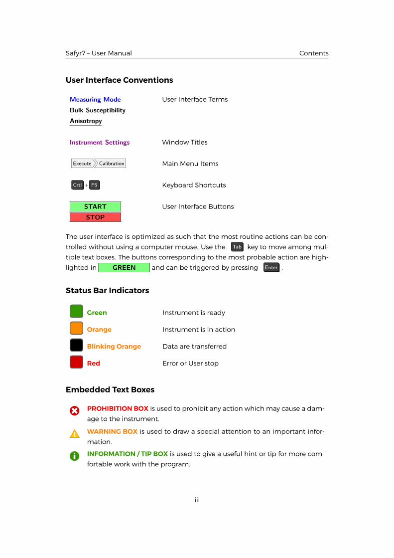
User Interface Conventions
Measuring Mode User Interface Terms
Bulk SusceptibilityAnisotropy
Instrument Settings Window Titles
Execute Calibration Main Menu Items
Crtl + F5 Keyboard Shortcuts
START User Interface Buttons
STOP
The user interface is optimized as such that the most routine actions can be con-
trolled without using a computer mouse. Use the Tab key to move among mul-
tiple text boxes. The buttons corresponding to the most probable action are high-
lighted in GREEN and can be triggered by pressing Enter .
Status Bar Indicators
Green Instrument is ready
Orange Instrument is in action
Blinking Orange Data are transferred
Red Error or User stop
Embedded Text Boxes
PROHIBITION BOX is used to prohibit any action which may cause a dam-
age to the instrument.
WARNING BOX is used to draw a special attention to an important infor-
mation.
INFORMATION / TIP BOX is used to give a useful hint or tip for more com-
fortable work with the program.
iii

Safyr7 – User Manual Contents
Please note that the appearance of the user interface may vary according to
the version of the operating system, language distribution and user settings. All
print-screens in this User Manual are based on Windows 10, English Distribu-tion with Default Settings.
iv
Safyr7 – User Manual Introduction
1 Introduction
Safyr7 is a Microsoft Windows computer program primarily designed to control
AGICOMFK1,MFK2, KLY5 series of Kappabridges (Table 1), optionally coupledwith
CS-3/4/L Temperature Control Units (Table 2). The program is based on a very in-
tuitive graphical user interface. The user interface offers two simultaneous working
regimes:
1. Instrument Control Regime – Enables an easy control over the whole array of
the sophisticated instrument measuring modes:
• AnisotropyofMagneticSusceptibility (AMS) –Magnetic anisotropymea-
sured using either the 15-position rotatable design or, in the case of the
automatic Kappabridge Versions (FA, A), using 1-Axis or two-axis (3D) Ro-
tator1. AMS can be measured in variable fields and, depending upon
the Kappabridge Model and Version (Table 1), at one or three operating
frequencies; KLY5 Model simultaneously determines both In-Phase and
Out-of-Phase anisotropy tensors.
• Bulk Susceptibility – Volume- or Mass-Normalized, In-Phase and Out-
of-Phase magnetic susceptibility measured in variable driving fields and,
depending upon the Kappabridge Model and Version (Table 1), at one or
three operating frequencies.
• TemperatureDependence – Magnetic susceptibilitymeasured as a func-
tion of temperature in the ”low” or ”high” temperature ranges (Table 2).2
Thermomagnetic curves can be measured in various fields and, depend-
ing upon theKappabridgeModel andVersion (Table 1), at one or three op-
erating frequencies; KLY5Model simultaneouslymeasures both In-Phase
and Out-of-Phase curves.
2. Data Viewing Regime3 – Enables an instant calculation and visualization the
results and basic data processing.
The acquired data are stored in binary or text files and can be visualized or further
processed using AGICO data processing computer programs Anisoft, Cureval, or
other programs of user’s choice.
1The 3D Rotator is an optional accessory to the automatic Kappabridge Versions.2The Kappabridge must be coupled with respective optional Temperature Control Unit(s).3The program can be used solely as a data viewer, i.e., without any instrument connected.
1
Safyr7 – User Manual Introduction
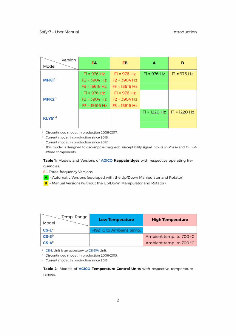
PPPPPPPPPPModel
VersionFA FB A B
F1 = 976 Hz F1 = 976 Hz F1 = 976 Hz F1 = 976 Hz
MFK1a F2 = 3904 Hz F2 = 3904 Hz
F3 = 15616 Hz F3 = 15616 Hz
F1 = 976 Hz F1 = 976 Hz
MFK2b F2 = 3904 Hz F2 = 3904 Hz
F3 = 15616 Hz F3 = 15616 Hz
F1 = 1220 Hz F1 = 1220 Hz
KLY5cd
a Discontinued model, in production 2006-2017.b Current model, in production since 2018.c Current model, in production since 2017.d This model is designed to decompose magnetic susceptibility signal into its In-Phase and Out-of-
Phase components.
Table 1: Models and Versions of AGICO Kappabridges with respective operating fre-
quencies.
F – Three-frequency Versions
A – Automatic Versions (equipped with the Up/Down Manipulator and Rotator)
B – Manual Versions (without the Up/Down Manipulator and Rotator)
XXXXXXXXXXXXXModel
Temp. RangeLow Temperature High Temperature
CS-La –192 ◦C to Ambient temp.
CS-3b Ambient temp. to 700 ◦C
CS-4c Ambient temp. to 700 ◦C
a CS-L Unit is an accessory to CS-3/4 Unit.b Discontinued model, in production 2006-2013.c Current model, in production since 2013.
Table 2: Models of AGICO Temperature Control Units with respective temperature
ranges.
2
Safyr7 – User Manual Getting Started
2 Getting Started
2.1 System Requirements
Safyr7 requires a PC computer with Microsoft Windows operating system (OS).
SupportedOS areWindows 10,Windows 8,Windows 7,WindowsVista,WindowsXP
in both 32 or 64-bit versions. Even though the program is supposed to work well in
various language versions, it is recommended that the English version used with a
decimal comma (”.”) set as the system decimal delimiter. For the best functionality
of the program, it is recommended that the default setting of the OS is used (i.e.,
no custom colors, enlarged font sizes, etc...)
2.2 Program Installation
Prior to the installation make sure that no other AGICO computer program is cur-
rently running. The actual installation procedure is very simple and follows the
usual steps of the Microsoft Windows software installation. You can navigate a step
forward or backward by clicking on Next > or < Back , respectively.
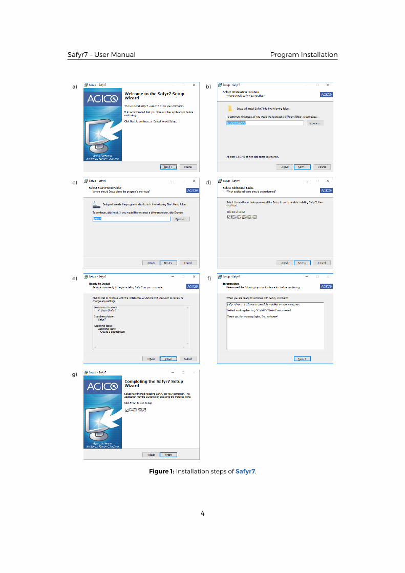
1. Double-click on Safyr7-Setup.exe to start the Safyr7 Setup Wizard (Figure 1a).
2. Select the installation directory (Figure 1b). It is recommended to keep the
default directory (C:\Agico\Safyr7) as pre-set by the installation wizard.
3. Choose the folder name in the Start menu (Figure 1c).
4. Indicate whether you want to create a desktop icon (Figure 1d).
5. Revise your installation settings and start the installation by clicking on Install(Figure 1e).
6. Revise the installation report (Figure 1f).
7. Finish the installation by clicking on Finish (Figure 1g).
To remove Safyr7 from your computer, go to the system Start Menu → (All Pro-
grams) → Safyr7 → Uninstall Safyr7 . When finished, all application files, desktop
icons, and shortcuts are deleted from the system.
3
Safyr7 – User Manual Program Installation
a) b)
c) d)
e) f)
g)
Figure 1: Installation steps of Safyr7.
4
Safyr7 – User Manual Program Execution
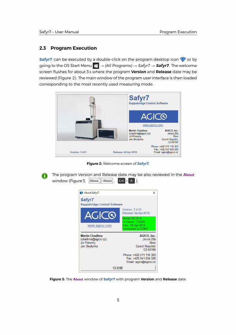
2.3 Program Execution
Safyr7 can be executed by a double-click on the program desktop icon or by
going to the OS Start Menu → (All Programs) → Safyr7 → Safyr7 . The welcome
screen flushes for about 3 s where the program Version and Release date may be
reviewed (Figure 2). Themain window of the program user interface is then loaded
corresponding to the most recently used measuring mode.
Figure 2: Welcome screen of Safyr7.
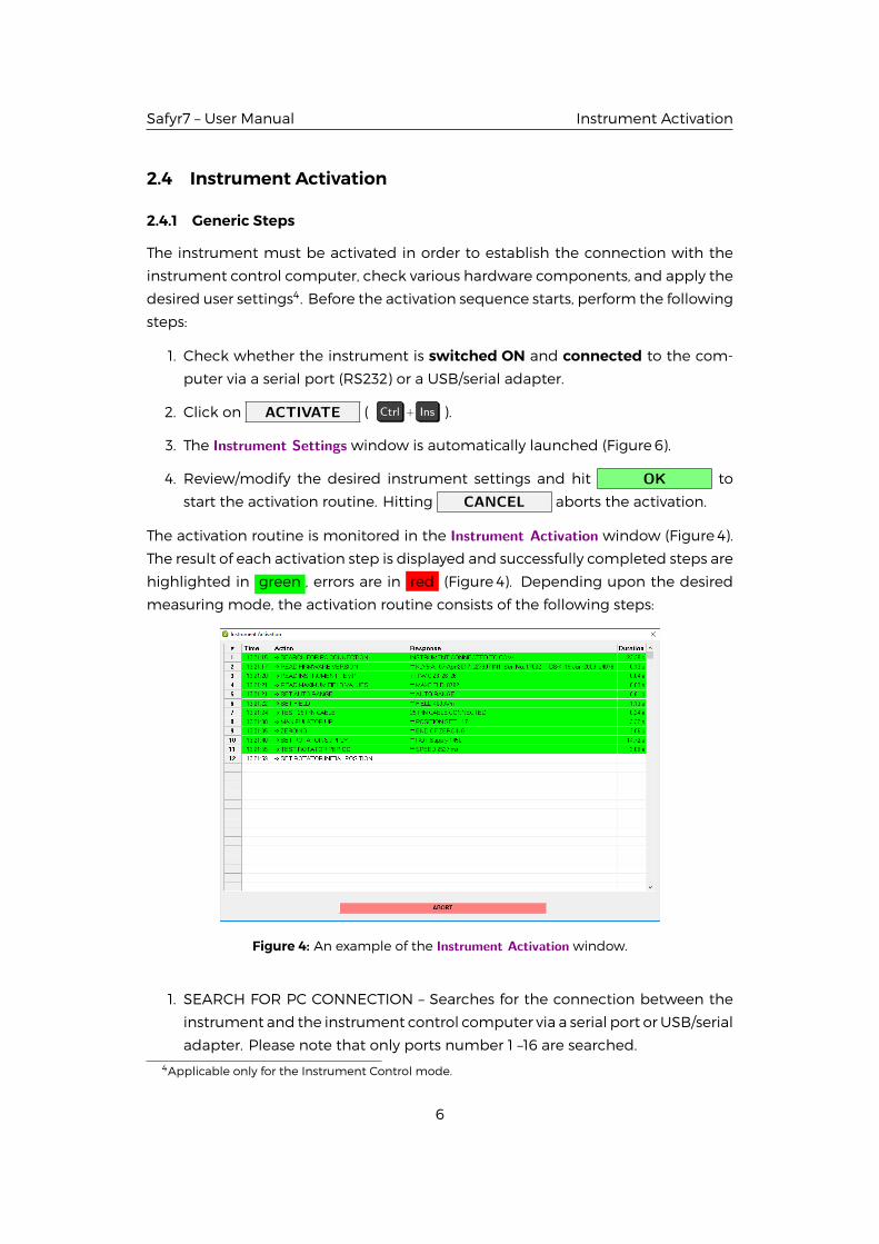
The program Version and Release date may be also reviewed in the Aboutwindow (Figure 3, About About , Crtl + A ).
Figure 3: The About window of Safyr7 with program Version and Release date.
5
Safyr7 – User Manual Instrument Activation
2.4 Instrument Activation
2.4.1 Generic Steps
The instrument must be activated in order to establish the connection with the
instrument control computer, check various hardware components, and apply the
desired user settings4. Before the activation sequence starts, perform the following
steps:
1. Check whether the instrument is switched ON and connected to the com-
puter via a serial port (RS232) or a USB/serial adapter.
2. Click on ACTIVATE ( Ctrl + Ins ).
3. The Instrument Settings window is automatically launched (Figure6).
4. Review/modify the desired instrument settings and hit OK to
start the activation routine. Hitting CANCEL aborts the activation.
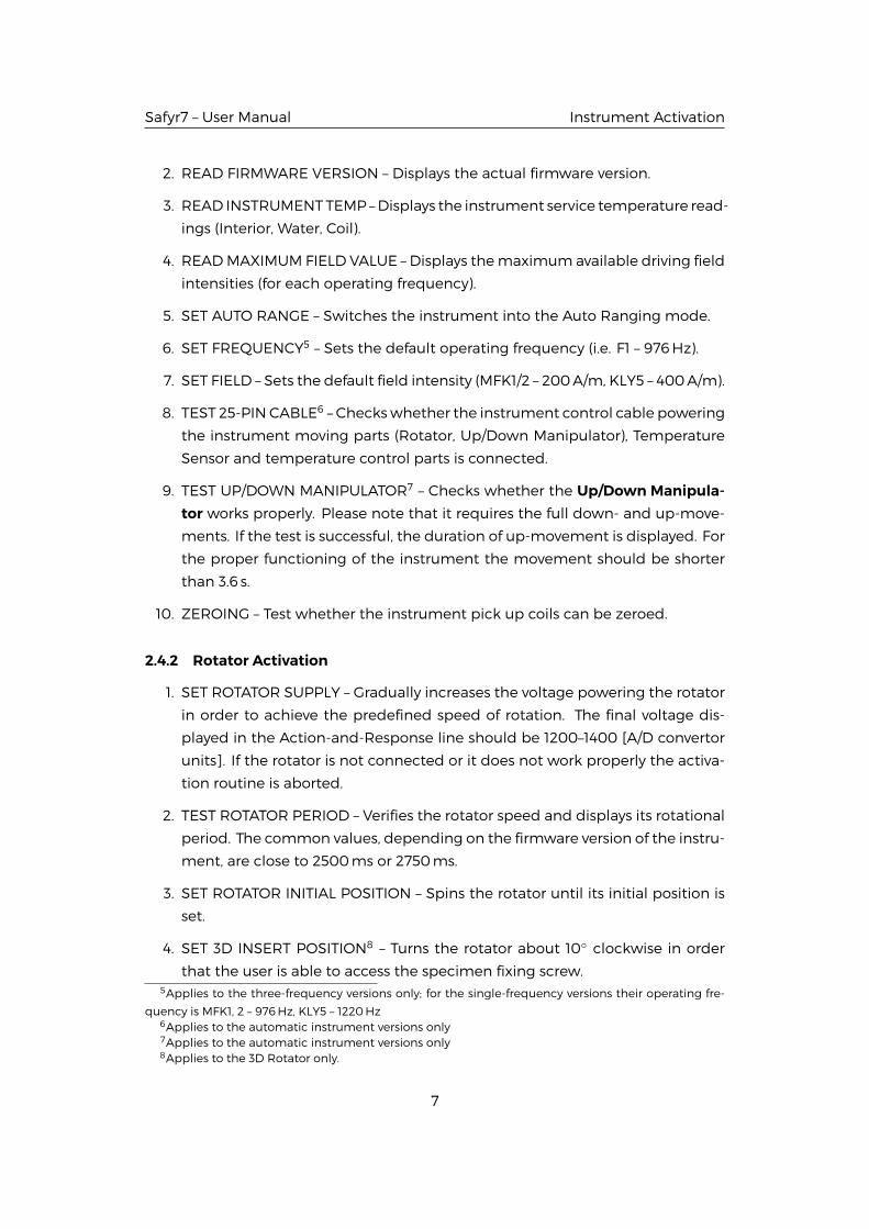
The activation routine is monitored in the Instrument Activation window (Figure 4).
The result of each activation step is displayed and successfully completed steps are
highlighted in green , errors are in red (Figure 4). Depending upon the desired
measuring mode, the activation routine consists of the following steps:
Figure 4: An example of the Instrument Activation window.
1. SEARCH FOR PC CONNECTION – Searches for the connection between the
instrument and the instrument control computer via a serial port or USB/serial
adapter. Please note that only ports number 1 –16 are searched.4Applicable only for the Instrument Control mode.
6
Safyr7 – User Manual Instrument Activation
2. READ FIRMWARE VERSION – Displays the actual firmware version.
3. READ INSTRUMENT TEMP –Displays the instrument service temperature read-
ings (Interior, Water, Coil).
4. READMAXIMUM FIELD VALUE – Displays themaximum available driving field
intensities (for each operating frequency).
5. SET AUTO RANGE – Switches the instrument into the Auto Ranging mode.
6. SET FREQUENCY5 – Sets the default operating frequency (i.e. F1 – 976Hz).
7. SET FIELD – Sets the default field intensity (MFK1/2 – 200A/m, KLY5 – 400A/m).
8. TEST 25-PIN CABLE6 – Checkswhether the instrument control cable powering
the instrument moving parts (Rotator, Up/Down Manipulator), Temperature
Sensor and temperature control parts is connected.
9. TEST UP/DOWN MANIPULATOR7 – Checks whether the Up/Down Manipula-tor works properly. Please note that it requires the full down- and up-move-
ments. If the test is successful, the duration of up-movement is displayed. For
the proper functioning of the instrument the movement should be shorter
than 3.6 s.
10. ZEROING – Test whether the instrument pick up coils can be zeroed.
2.4.2 Rotator Activation
1. SET ROTATOR SUPPLY – Gradually increases the voltage powering the rotator
in order to achieve the predefined speed of rotation. The final voltage dis-
played in the Action-and-Response line should be 1200–1400 [A/D convertor
units]. If the rotator is not connected or it does not work properly the activa-
tion routine is aborted.
2. TEST ROTATOR PERIOD – Verifies the rotator speed and displays its rotational
period. The common values, depending on the firmware version of the instru-
ment, are close to 2500ms or 2750ms.
3. SET ROTATOR INITIAL POSITION – Spins the rotator until its initial position is
set.
4. SET 3D INSERT POSITION8 – Turns the rotator about 10◦ clockwise in order
that the user is able to access the specimen fixing screw.5Applies to the three-frequency versions only; for the single-frequency versions their operating fre-
quency is MFK1, 2 – 976Hz, KLY5 – 1220Hz6Applies to the automatic instrument versions only7Applies to the automatic instrument versions only8Applies to the 3D Rotator only.
7
Safyr7 – User Manual Instrument Activation
2.4.3 Temperature Control Unit Activation
The following steps are performed only when Temperature Dependence Mode is
set and Temperature Sensor is connected.
NEVER Connect/Disconnect Temperature Sensor to/from the Pick Up
Unit when the instrument is switched ON! It may cause a short circuit
harmful to the instrument. Always switch the instrument OFF when ma-
nipulating with Temperature Sensor connection.
1. ACTIVATE CS UNIT – Activates the Temperature Control Unit (CS) and auto-
matically detects the Low or High Temperature Mode according to whether
Cryostat is connected or not, respectively.
2. READ SPECIMEN TEMP – Checks whether the temperature sensor works cor-
rectly and displays its temperature reading.
3. CHECK WATER FLOW9 – Checks whether the cooling water close circuit pro-
vides enough water necessary to cool down the exterior of the furnace.
4. CHECK HEATING – Checks the heating wiring Current [A] and Voltage [V].
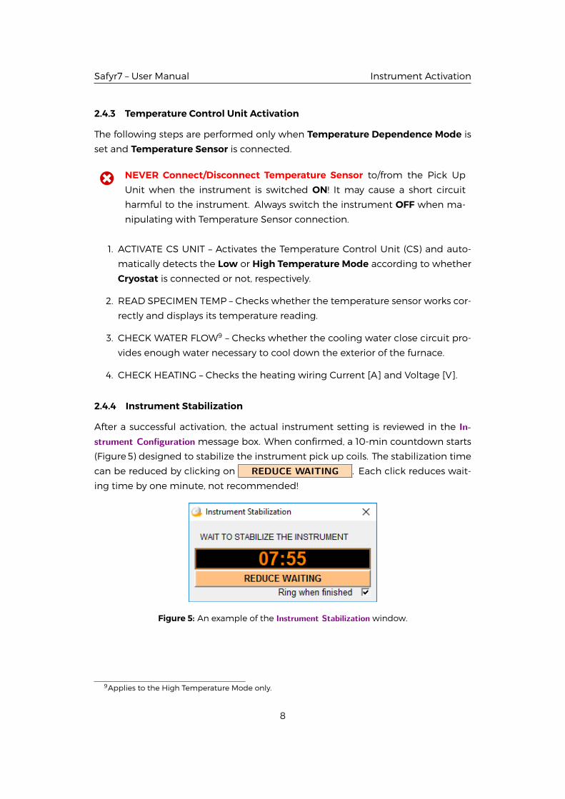
2.4.4 Instrument Stabilization
After a successful activation, the actual instrument setting is reviewed in the In-strument Configuration message box. When confirmed, a 10-min countdown starts
(Figure 5) designed to stabilize the instrument pick up coils. The stabilization time
can be reduced by clicking on REDUCE WAITING . Each click reduces wait-
ing time by one minute, not recommended!
Figure 5: An example of the Instrument Stabilization window.
9Applies to the High Temperature Mode only.
8
Safyr7 – User Manual Settings
3 Settings
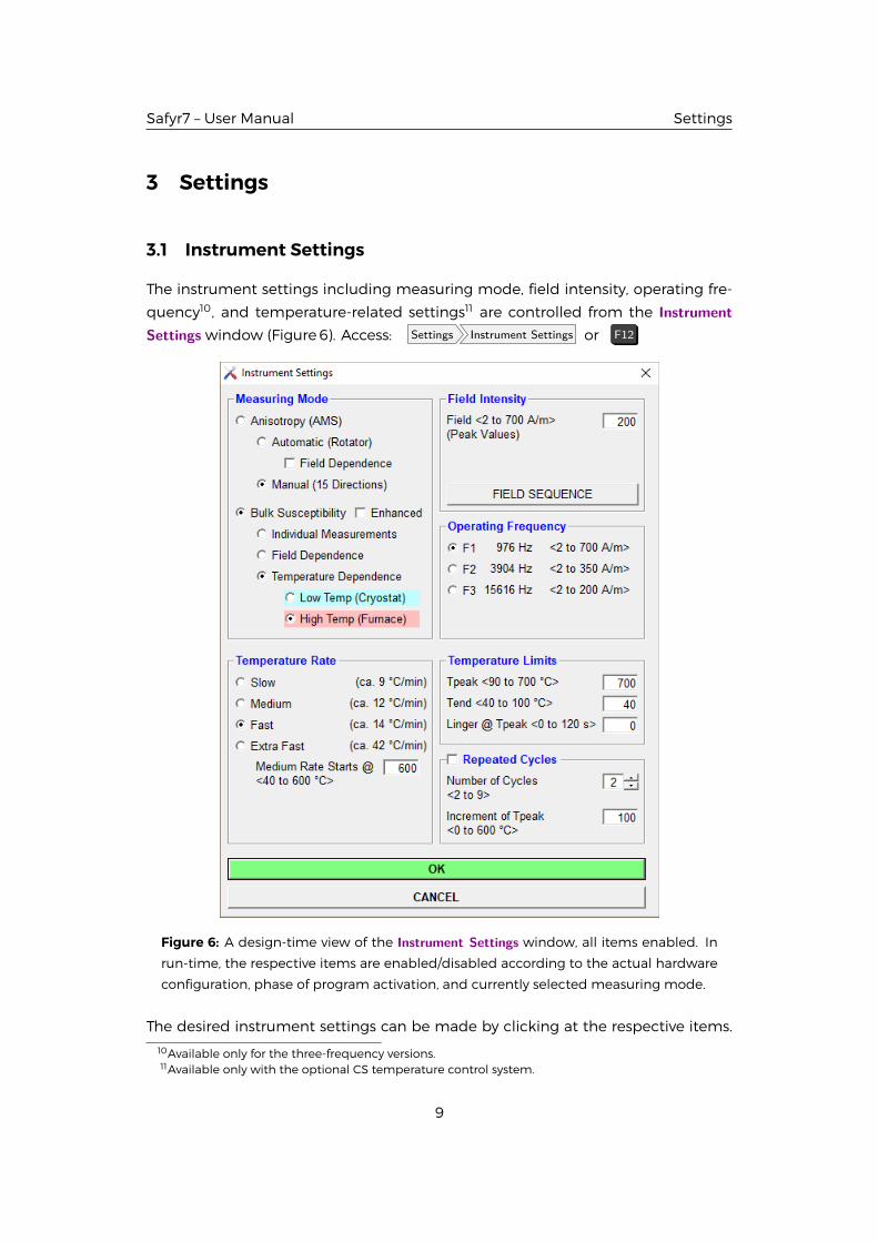
3.1 Instrument Settings
The instrument settings including measuring mode, field intensity, operating fre-
quency10, and temperature-related settings11 are controlled from the InstrumentSettings window (Figure6). Access: Settings Instrument Settings or F12
Figure 6: A design-time view of the Instrument Settings window, all items enabled. In
run-time, the respective items are enabled/disabled according to the actual hardware
configuration, phase of program activation, and currently selected measuring mode.
The desired instrument settings can be made by clicking at the respective items.
10Available only for the three-frequency versions.11Available only with the optional CS temperature control system.
9
Safyr7 – User Manual Instrument Settings
When done:
• Click OK to apply the desired settings. The activation routine is
monitored in the Instrument Activation window. The actual measuring proce-
dures are described in details in Chapter 5.
• Click CANCEL to close thewindowwith the previous settings retained.
3.1.1 Measuring Mode
Depending on the actual hardware configuration, Safyr7 may work in six different
measuring modes:
Anisotropy of Magnetic Susceptibility (AMS)
1. Automatic Anisotropy Mode
2. Manual Anisotropy Mode
Bulk Susceptibility
3. Individual Measurements Mode
4. Field Dependence Mode
Temperature Dependence
5. Low Temperature Mode
6. High Temperature Mode
3.1.1.1 Automatic AnisotropyMode 12 controls the automatic AMSmeasurements
of the spinning specimen using 1-Axis Rotator or 3D Rotator. The measurements
can be performed in desired field intensity (see Section 3.1.2.1) and, if applicable, in
various operating frequencies (see Section 3.1.3).
To set this mode:
1. Check whether 1-Axis Rotator or 3DRotator is connected to the Pick Up Unit.
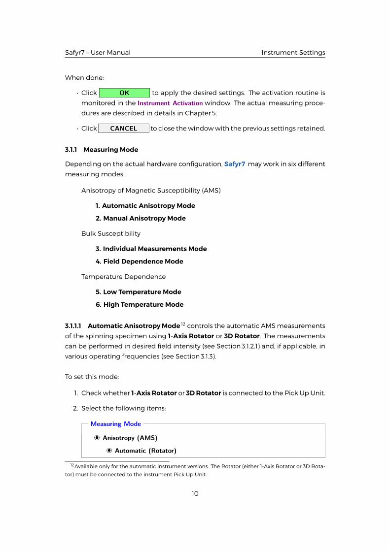
2. Select the following items:
Measuring Mode
Anisotropy (AMS)
Automatic (Rotator)
12Available only for the automatic instrument versions. The Rotator (either 1-Axis Rotator or 3D Rota-
tor) must be connected to the instrument Pick Up Unit.
10
Safyr7 – User Manual Instrument Settings
3. Hit OK to confirm.
4. The activation routine follows the same steps as described in Section2.4.2 and
automatically recognizes whether 1-Axis Rotator or 3D Rotator is connectedto the instrument Pick Up Unit and sets the user interface accordingly.
The actual measuring procedure is described in details in Section5.2, Page42.
NEVERCONNECT/DISCONNECTROTATOR to/from the Pick Up Unit when
the instrument is switched ON! This illegal action may cause a short circuit
harmful to the instrument. Before connecting/disconnecting the Rotator,
exit Safyr7and switch the instrument OFF.
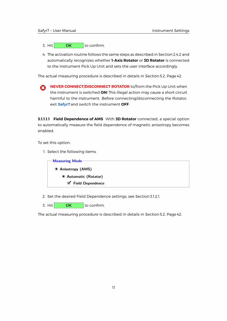
3.1.1.1.1 Field Dependence of AMS With 3D Rotator connected, a special option
to automatically measure the field dependence of magnetic anisotropy becomes
enabled.
To set this option:
1. Select the following items:
Measuring Mode
Anisotropy (AMS)
Automatic (Rotator)�D Field Dependence
2. Set the desired Field Dependence settings, see Section 3.1.2.1.
3. Hit OK to confirm.
The actual measuring procedure is described in details in Section5.2, Page42.
11
Safyr7 – User Manual Instrument Settings
3.1.1.2 ManualAnisotropyMode provides an option tomeasureAMS tensorsman-
ually based on fifteen directional susceptibility measurements following the rotat-
able design of Jelinek. The measurements can be performed in desired field in-
tensity (see Section 3.1.2.1) and, if applicable, in various operating frequencies (see
Section 3.1.3).
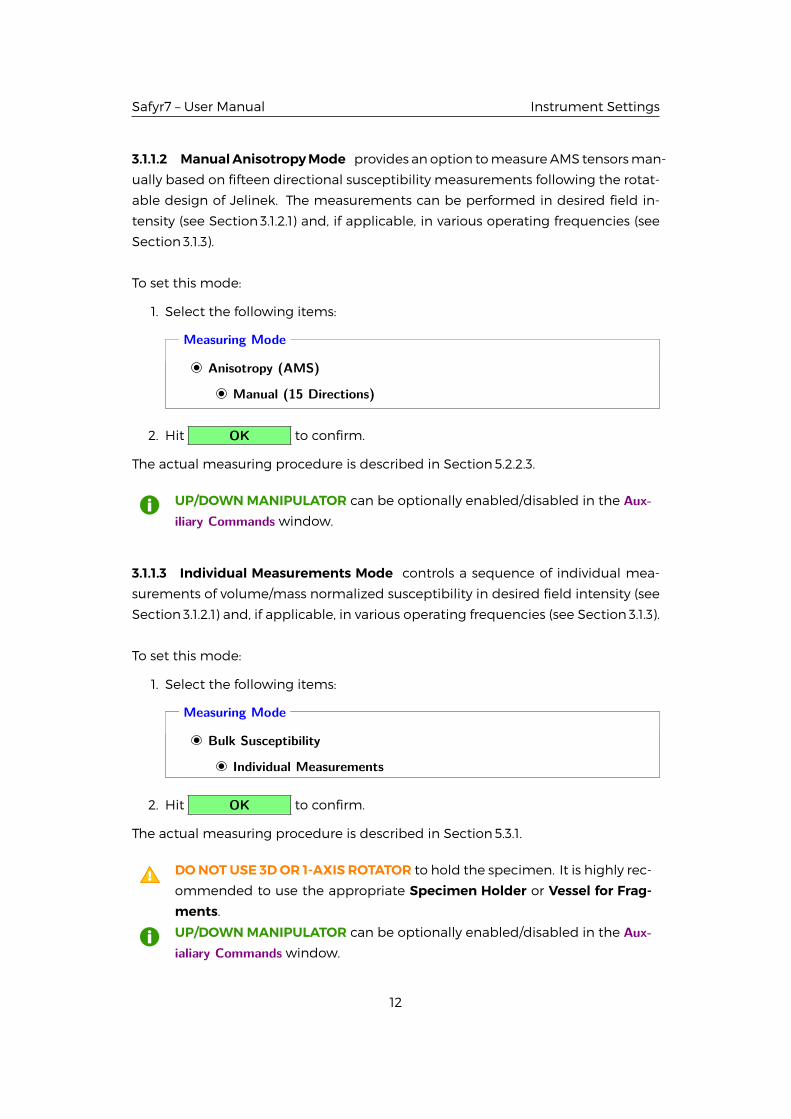
To set this mode:
1. Select the following items:
Measuring Mode
Anisotropy (AMS)
Manual (15 Directions)
2. Hit OK to confirm.
The actual measuring procedure is described in Section5.2.2.3.
UP/DOWN MANIPULATOR can be optionally enabled/disabled in the Aux-iliary Commands window.
3.1.1.3 Individual Measurements Mode controls a sequence of individual mea-
surements of volume/mass normalized susceptibility in desired field intensity (see
Section 3.1.2.1) and, if applicable, in various operating frequencies (see Section 3.1.3).
To set this mode:
1. Select the following items:
Measuring Mode
Bulk Susceptibility
Individual Measurements
2. Hit OK to confirm.
The actual measuring procedure is described in Section5.3.1.
DONOTUSE 3DOR 1-AXIS ROTATOR to hold the specimen. It is highly rec-
ommended to use the appropriate Specimen Holder or Vessel for Frag-ments.
UP/DOWN MANIPULATOR can be optionally enabled/disabled in the Aux-ialiary Commands window.
12
Safyr7 – User Manual Instrument Settings
3.1.1.3.1 Enhanced Drift Compensation Measurement In order to enhance the
drift compensation algorithm, eachmeasurement may be performed in two steps
(two subsequent down and up motions):
1. Finds the appropriate measuring range.
2. Measures the specimen in the fixed range in which the finest drift compen-
sation can be achieved.
To select this option:
• Check �DEnhanced
PLEASE NOTE that each measurement takes double time compared to
the regular (one-step) algorithm in which the automatic instrument rang-
ing routine is used. For that reason, this optionmay be applied only for the
Individual Measurements and Field Dependence Modes
3.1.1.4 FieldDependenceMode controls themeasurements of volume/mass nor-
malized susceptibility as a function of field intensity. If applicable, the measure-
ments canbeperformed in various operating frequencies (see Section 3.1.3, Page24).
To set this mode:
1. Select the following items:
Measuring Mode
Bulk Susceptibility
Field Dependence
2. To set the desired Field Dependence settings, see Section 3.1.2.1.
3. Hit OK to confirm.
The actual measuring routine is described in Section5.3.2.
DONOTUSE 3DOR 1-AXIS ROTATOR to hold the specimen. It is highly rec-
ommended to use the appropriate Specimen Holder or Vessel for Frag-ments.
UP/DOWN MANIPULATOR can be optionally enabled/disabled in the Aux-ialiary Commands window.
13
Safyr7 – User Manual Instrument Settings
3.1.1.5 Low Temperature Mode controls the acquisition of thermomagnetic cur-
ves (variation of magnetic susceptibility as a function of temperature) in the so-
called low temperature range (−192 ◦C to ambient temperature) using Cryostat.Prior to the measurement, the powder specimen is cooled down to the tempera-
ture close to that of liquid nitrogen. The specimen is then heated spontaneously
up to the desiredmaximum temperaturewhilemagnetic susceptibility is recorded
approx. every 20 s.
To set this mode:
1. Check whether Temperature Sensor is connected to the Pick Up Unit.
2. Check whether Cryostat is installed and connected to the Pick Up Unit.
3. Select the following items:
Measuring Mode
Bulk Susceptibility
Temperature DependenceLow Temp (Cryostat)
4. Set desired Temperature Limits.
5. Hit OK to confirm.
6. The activation routine follows the same steps as described in Section2.4.2.
Please note that the instrument is activated in Low Temperature Mode only
when Cryostat is connected to the Pick Up Unit.
NEVER CONNECT/DISCONNECT TEMPERATURE SENSOR to/from the
Pick Up Unit when the instrument is switched ON! This illegal action
may cause a short circuit harmful to the instrument. Before connect-
ing/disconnecting Temperature Sensor, exit Safyr7and switch the instru-
ment OFF.
DO NOT CONNECT/DISCONNECT CRYOSTAT to/from the Pick Up Unit
when the Temperature Control Unit (CS) is activated! This illegal action
generates firmware error xxx (accompanied by an acoustic warning) and
results in instrument deactivation. Prior reactivation, switch the instrument
OFF and ON to clear the error warning.
14
Safyr7 – User Manual Instrument Settings
SWAPPING TEMPERATURE MODES from High Temperature into LowTemperature can be executed as follows:
1. Select Low Temp (Cryostat)
2. Hit OK .
3. The Temperature Control Unit (CS) is deactivated.
4. When prompted, uninstall Furnace and install and connect Cryostat.
5. Hit OK .
6. The Temperature Control Unit (CS) is activated in Low TemperatureMode.
3.1.1.5.1 Temperature Limits Set the temperature limits bymanual input into the
respective text boxes:
1. Set Tstart – Temperature at which the user is allowed to start the measure-
ment.
Input range ⟨−192 ◦C to 0 ◦C⟩
2. Set Tend – Temperature at which the measurement is terminated.
Input range ⟨0 to 25 ◦C⟩
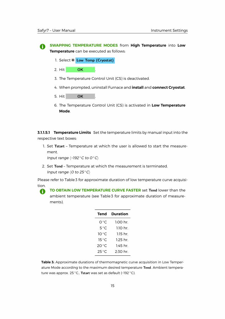
Please refer to Table 3 for approximate duration of low temperature curve acquisi-
tion.TO OBTAIN LOW TEMPERATURE CURVE FASTER set Tend lower than the
ambient temperature (see Table 3 for approximate duration of measure-
ments).
Tend Duration
0 ◦C 1:00 hr.
5 ◦C 1:10 hr.
10 ◦C 1:15 hr.
15 ◦C 1:25 hr.
20 ◦C 1:45 hr.
25 ◦C 2:30 hr.
Table 3: Approximate durations of thermomagnetic curve acquisition in Low Temper-
ature Mode according to the maximum desired temperature Tend. Ambient tempera-
ture was approx. 25 ◦C., Tstart was set as default (−192 ◦C).
15
Safyr7 – User Manual Instrument Settings
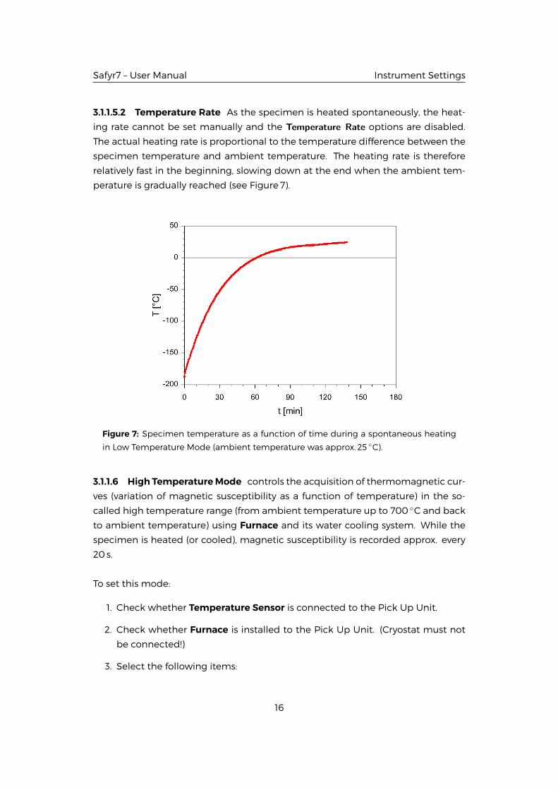
3.1.1.5.2 Temperature Rate As the specimen is heated spontaneously, the heat-
ing rate cannot be set manually and the Temperature Rate options are disabled.
The actual heating rate is proportional to the temperature difference between the
specimen temperature and ambient temperature. The heating rate is therefore
relatively fast in the beginning, slowing down at the end when the ambient tem-
perature is gradually reached (see Figure 7).
Figure 7: Specimen temperature as a function of time during a spontaneous heating
in Low Temperature Mode (ambient temperature was approx. 25 ◦C).
3.1.1.6 High TemperatureMode controls the acquisition of thermomagnetic cur-
ves (variation of magnetic susceptibility as a function of temperature) in the so-
called high temperature range (from ambient temperature up to 700 ◦C and back
to ambient temperature) using Furnace and its water cooling system. While the
specimen is heated (or cooled), magnetic susceptibility is recorded approx. every
20 s.
To set this mode:
1. Check whether Temperature Sensor is connected to the Pick Up Unit.
2. Check whether Furnace is installed to the Pick Up Unit. (Cryostat must not
be connected!)
3. Select the following items:
16
Safyr7 – User Manual Instrument Settings
Measuring Mode
Bulk Susceptibility
Temperature DependenceHigh Temp (Furnace)
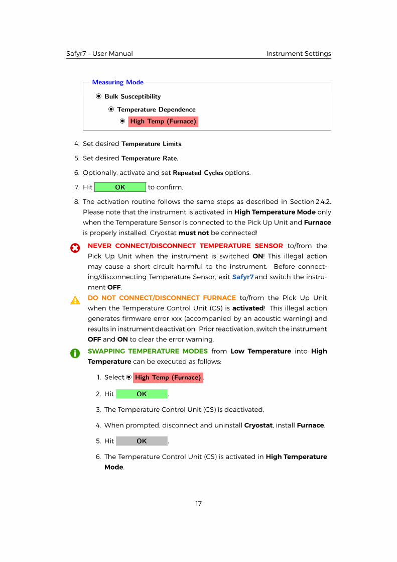
4. Set desired Temperature Limits.
5. Set desired Temperature Rate.
6. Optionally, activate and set Repeated Cycles options.
7. Hit OK to confirm.
8. The activation routine follows the same steps as described in Section2.4.2.
Please note that the instrument is activated in High Temperature Mode only
when the Temperature Sensor is connected to the Pick Up Unit and Furnaceis properly installed. Cryostat must not be connected!
NEVER CONNECT/DISCONNECT TEMPERATURE SENSOR to/from the
Pick Up Unit when the instrument is switched ON! This illegal action
may cause a short circuit harmful to the instrument. Before connect-
ing/disconnecting Temperature Sensor, exit Safyr7and switch the instru-
ment OFF.
DO NOT CONNECT/DISCONNECT FURNACE to/from the Pick Up Unit
when the Temperature Control Unit (CS) is activated! This illegal action
generates firmware error xxx (accompanied by an acoustic warning) and
results in instrument deactivation. Prior reactivation, switch the instrument
OFF and ON to clear the error warning.
SWAPPING TEMPERATURE MODES from Low Temperature into HighTemperature can be executed as follows:
1. Select High Temp (Furnace) .
2. Hit OK .
3. The Temperature Control Unit (CS) is deactivated.
4. When prompted, disconnect and uninstall Cryostat, install Furnace.
5. Hit OK .
6. The Temperature Control Unit (CS) is activated in High TemperatureMode.
17

Safyr7 – User Manual Instrument Settings
3.1.1.6.1 Temperature Limits In High Temperature Mode, the specimen is heated
from the ambient temperature up to the desired peak temperature (heating half-
cycle) and then cooled down to the desired end temperature (cooling half-cycle)
while magnetic susceptibility is recorded approx. every 20 s.
Set the temperature limits by manual input into the respective text boxes:
1. Set Tpeak – Upper temperature limit to which the specimen is heated in the
heating half-cycle.
Input range ⟨90 to 700 ◦C⟩
2. Set Tend – Temperature below which the cooling half-cycle is terminated.
Input range ⟨40 to 100 ◦C⟩
3. Optionally set Linger @ Tpeak – Time duringwhich Tpeak temperature ismain-
tained in the end of heating half-cycle.
Input range ⟨0 to 120 s⟩
3.1.1.6.2 Temperature Rate In High Temperature Mode, the specimen is heated
at a controlled rate to the maximum temperature Tpeak and then cooled down
at the same rate to the minimum temperature Tend. There are four temperature
rates available (Figure 9). Default temperature rate (Fast) is suitable for most rocks
and environmental materials. For special studies, slower temperature rates (Slow,
Medium) can be used but one must realize that such measurements take corre-
spondingly longer time (see Table 4).
18

Safyr7 – User Manual Instrument Settings
Figure 8: Specimen temperature as a function of time for four available temperature
rates in the High Temperature Mode.
TO OBTAIN HIGH TEMPERATURE CURVE FASTER use the Extra Fast tem-
perature rate (ca. 42 ◦C/min). This option may be especially useful when
one is not interested in a whole course of thermomagnetic curve but only
in a fast way to obtained characteristic temperature(s), e.g., Curie points. In
order to havemoremeasurements in the high temperature interval where
the characteristic temperature is expected to be, the heating rate is slowed
down (roughly corresponding to Medium Rate) when the desired Tpeak is
approached. The temperature above which Medium Rate Starts is set auto-matically or manually; it should be at least 100 ◦C below the desired Tpeaktemperature.
Temperature Rate Duration
Slow 9 ◦C/min 2:45 hr.
Medium 12 ◦C/min 2:00 hr.
Fast 14 ◦C/min 1:45 hr.
Extra Fast 42 ◦C/min 1:00 hr.
Table 4: Temperature rates available in the High TempearatureModewith approximate
duration of a standardmeasurement cycle (from the ambient temperature up to 700 ◦C
and down to 40 ◦C). Default temperature rate is in bold.
19

Safyr7 – User Manual Instrument Settings
3.1.1.6.3 Repeated Cycles In the High Temperature Mode, several subsequent
heating/cooling cycles can be automatically measured. For each cycle, the peak
temperature (Tpeak) is automatically increased by a desired temperature incre-
ment.
To apply this option:
1. Set Temperature Limits for the first heating/cooling cycle, see Section 3.1.1.6.1
2. Check �DRepeated Cycles
3. Set Number of Cycles – Number of heating/cooling cycles.
Input range ⟨2 to 9⟩
4. Set Increment of Tpeak – Increment by which Tpeak is increased in each heat-
ing/cooling cycle.
Input range ⟨0 to 600 ◦C⟩
Example of settings:
• Tpeak = 100
• Tend = 40
• Linger @ Tpeak = 60
• Number of Cycles = 5
• Increment of Tpeak = 100
This setting results in 5 heating/cooling cycles:
1. Heating ⟨Ambient temp. to 100 ◦C⟩ → Linger 60 s → Cooling ⟨100 to 40 ◦C⟩
2. Heating ⟨40 to 200 ◦C⟩ → Linger 60 s → Cooling ⟨200 to 40 ◦C⟩
3. Heating ⟨40 to 300 ◦C⟩ → Linger 60 s → Cooling ⟨300 to 40 ◦C⟩
4. Heating ⟨40 to 400 ◦C⟩ → Linger 60 s → Cooling ⟨400 to 40 ◦C⟩
5. Heating ⟨40 to 500 ◦C⟩ → Linger 60 s → Cooling ⟨500 to 40 ◦C⟩
20
Safyr7 – User Manual Instrument Settings
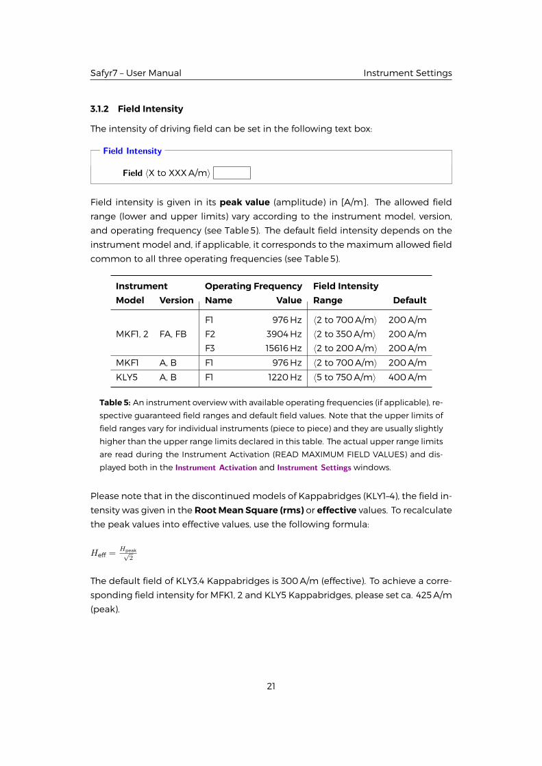
3.1.2 Field Intensity
The intensity of driving field can be set in the following text box:
Field Intensity
Field ⟨X to XXXA/m⟩
Field intensity is given in its peak value (amplitude) in [A/m]. The allowed field
range (lower and upper limits) vary according to the instrument model, version,
and operating frequency (see Table 5). The default field intensity depends on the
instrument model and, if applicable, it corresponds to themaximum allowed field
common to all three operating frequencies (see Table 5).
Instrument Operating Frequency Field IntensityModel Version Name Value Range Default
F1 976Hz ⟨2 to 700A/m⟩ 200A/m
MKF1, 2 FA, FB F2 3904Hz ⟨2 to 350A/m⟩ 200A/m
F3 15616Hz ⟨2 to 200A/m⟩ 200A/m
MKF1 A, B F1 976Hz ⟨2 to 700A/m⟩ 200A/m
KLY5 A, B F1 1220Hz ⟨5 to 750A/m⟩ 400A/m
Table 5: An instrument overviewwith available operating frequencies (if applicable), re-
spective guaranteed field ranges and default field values. Note that the upper limits of
field ranges vary for individual instruments (piece to piece) and they are usually slightly
higher than the upper range limits declared in this table. The actual upper range limits
are read during the Instrument Activation (READ MAXIMUM FIELD VALUES) and dis-
played both in the Instrument Activation and Instrument Settings windows.
Please note that in the discontinuedmodels of Kappabridges (KLY1–4), the field in-
tensity was given in the RootMean Square (rms) or effective values. To recalculate
the peak values into effective values, use the following formula:
Heff =Hpeak√
2
The default field of KLY3,4 Kappabridges is 300A/m (effective). To achieve a corre-
sponding field intensity for MFK1, 2 and KLY5 Kappabridges, please set ca. 425A/m
(peak).
21
Safyr7 – User Manual Instrument Settings
3.1.2.1 FieldDependence Field dependence settings are applicable for both field
dependence of bulk susceptibility and field dependence of magnetic anisotropy.
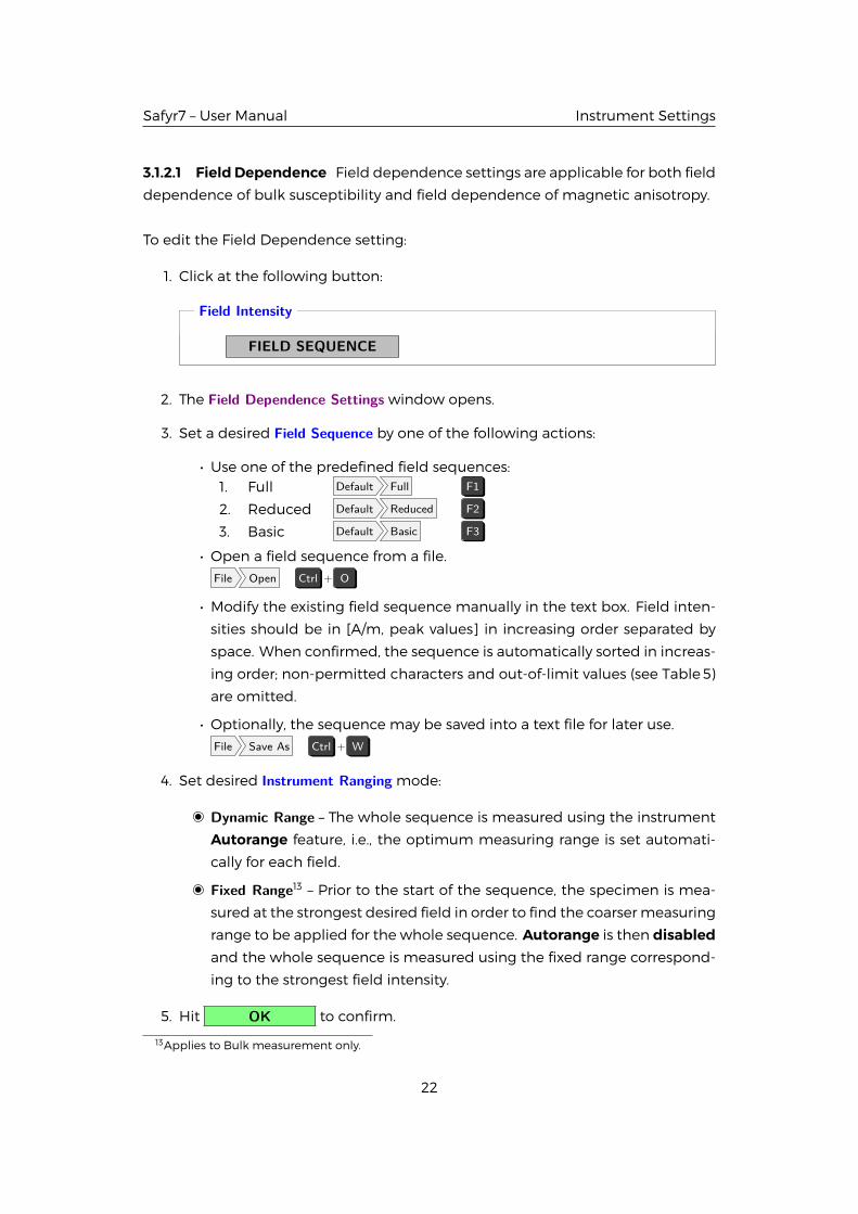
To edit the Field Dependence setting:
1. Click at the following button:
Field Intensity
FIELD SEQUENCE
2. The Field Dependence Settings window opens.
3. Set a desired Field Sequence by one of the following actions:
• Use one of the predefined field sequences:1. Full Default Full F1
2. Reduced Default Reduced F2
3. Basic Default Basic F3
• Open a field sequence from a file.File Open Ctrl + O
• Modify the existing field sequence manually in the text box. Field inten-
sities should be in [A/m, peak values] in increasing order separated by
space. When confirmed, the sequence is automatically sorted in increas-
ing order; non-permitted characters and out-of-limit values (see Table 5)
are omitted.
• Optionally, the sequence may be saved into a text file for later use.File Save As Ctrl + W
4. Set desired Instrument Ranging mode:
Dynamic Range – The whole sequence is measured using the instrument
Autorange feature, i.e., the optimum measuring range is set automati-
cally for each field.
Fixed Range13 – Prior to the start of the sequence, the specimen is mea-
sured at the strongest desired field in order to find the coarsermeasuring
range to be applied for the whole sequence. Autorange is then disabledand the whole sequence is measured using the fixed range correspond-
ing to the strongest field intensity.
5. Hit OK to confirm.
13Applies to Bulk measurement only.
22
Safyr7 – User Manual Instrument Settings
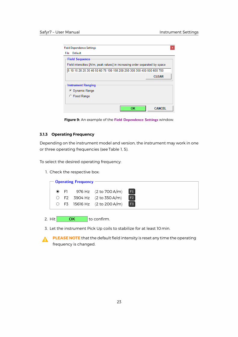
Figure 9: An example of the Field Dependence Settings window.
3.1.3 Operating Frequency
Depending on the instrumentmodel and version, the instrumentmay work in one
or three operating frequencies (see Table 1, 5).
To select the desired operating frequency:
1. Check the respective box:
Operating Frequency
F1 976 Hz ⟨2 to 700A/m⟩ F1
F2 3904 Hz ⟨2 to 350A/m⟩ F2
F3 15616 Hz ⟨2 to 200A/m⟩ F3
2. Hit OK to confirm.
3. Let the instrument Pick Up coils to stabilize for at least 10min.
PLEASENOTE that the default field intensity is reset any time the operating
frequency is changed.
23
Safyr7 – User Manual Volume / Mass Susceptibility
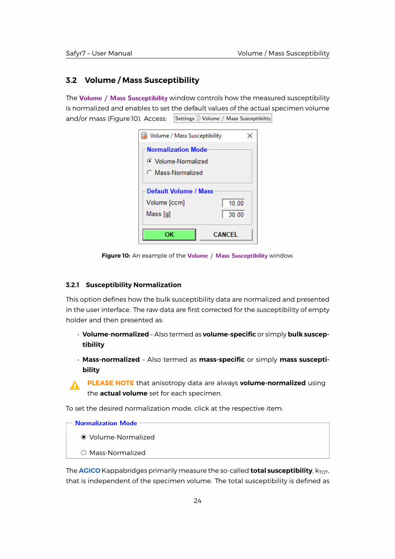
3.2 Volume / Mass Susceptibility
The Volume / Mass Susceptibility window controls how the measured susceptibility
is normalized and enables to set the default values of the actual specimen volume
and/or mass (Figure 10). Access: Settings Volume / Mass Susceptibility
Figure 10: An example of the Volume / Mass Susceptibility window.
3.2.1 Susceptibility Normalization
This option defines how the bulk susceptibility data are normalized and presented
in the user interface. The raw data are first corrected for the susceptibility of empty
holder and then presented as:
• Volume-normalized – Also termed as volume-specific or simplybulk suscep-tibility
• Mass-normalized – Also termed as mass-specific or simply mass suscepti-bility
PLEASE NOTE that anisotropy data are always volume-normalized using
the actual volume set for each specimen.
To set the desired normalization mode, click at the respective item:
Normalization Mode
Volume-Normalized
Mass-Normalized
TheAGICOKappabridges primarilymeasure the so-called total susceptibility, kTOT,
that is independent of the specimen volume. The total susceptibility is defined as
24
Safyr7 – User Manual Volume / Mass Susceptibility
the induced magnetic moment of the specimen divided by the nominal volume
of the instrument (being 10cm3 for AGICOKappabridges). The total susceptibility
is very convenient in sensitivity and error considerations because it directly corre-
sponds to the ”raw susceptibility signal” provided by the instrument.
The volume-normalized susceptibility, kVOL, is calculated as follows:
kVOL =V0
VkTOT
where V is the actual volume of the specimen and V0 is the nominal volume (V0=
10cm3).
The volume-normalized susceptibility is presented in dimensionless SI unit.
In environmentalmagnetism, themass-normalized susceptibility, χ, is often used.
It is related to the volume-normalized susceptibility as follows:
χ =kVOL
ρ=
VkVOL
m
where ρ is density, m is specimen mass.
The mass-normalized susceptibility is then related to the total susceptibility as fol-
lows:
χ =V0
VVm
kTOT =V0
mkTOT,
The mass-normalized susceptibility is presented in [m3/kg].
3.2.2 Default Volume / Mass
The Default specimen volume or mass value is used each time a new measure-
ment is started and displayed in the New Specimen window where the user may
overwrite it with the Actual volume or mass value.
The default volume and mass is set by direct input in the respective text boxes:
Default Volume / Mass
Volume [ccm] ⟨1 to 20cm3⟩Mass [g] ⟨0.01 to 40g⟩
25
Safyr7 – User Manual Anisotropy Settings
3.3 Anisotropy Settings
The following settings are available only whenMagneticAnisotropymodes are set.
3.3.1 Demagnetizing Factor
This option indicates whether the correction for demagnetizing factor is consid-
ered in the calculation of mean susceptibility.
To enable this option:
1. Click at Settings Anisotropy Settings Use Demagnetizing Factor .
2. Go to Settings Anisotropy Settings and check whetherDcheckmark appears in
front of DUse Demagnetizing Factor item.
To disable this option:
1. Click at Settings Anisotropy Settings Use Demagnetizing Factor .
2. Go to Settings Anisotropy Settings and check whether no check mark appears
in front of Use Demagnetizing Factor item.
3.3.2 Orientation Parameters
In general, there are multiple ways how to sample the oriented specimens. Safyr7adapts the general transformation matrix to transform the acquired anisotropy
data from the specimen coordinate system into geographic coordinate system
(and tectonic coordinate systems) using a set of Orientation Parameters (P1, P2,P3, P4). The Orientation Parameters quantitatively describe the sampling scheme
(see Figure 35 in Appendix).
To set the appropriate Orientation Parameters:
1. Go to: Settings Anisotropy Settings Orientation Parameters to launch the OrientationParameters window.
2. Verify the current settings of Orientation Parameters.
3. To enable any changes, hit CHANGE .
4. Select the Orientation Parameters.
5. Hit OK to confirm.
26

Safyr7 – User Manual Anisotropy Settings
3.3.3 Quantitative Anisotropy Factors
There is a set of eight Quantitative Anisotropy Factors which are calculated and
displayed in the user interface. For the definitions of available Anisotropy Factors,
go to Section 6.3 in Appendix, Page 79).
To select the desired Anisotropy Factors:
1. Go to: Settings Anisotropy Settings Quantitative Anisotropy Factors to launch theQuan-titative Anisotropy Factors window (Figure 11).
2. Verify the current settings of Anisotropy Factors.
3. To enable any changes, hit CHANGE .
4. For each Factor, selected from 38 predefined equations and enter the desired
Factor name.
5. Hit OK to confirm.
Figure 11: An example of the Quantitative Anisotropy Factors window.
PLEASE NOTE that no Quantitative Anisotropy Factors are stored in the
anisotropy data files (*.ams, *.ran). These data files store only the tensor
elements and the Anisotropy Factors are calculated during the subsequent
data processing according to the setting in the data processing software.
27

Safyr7 – User Manual Auxiliary Routines
4 Auxiliary Routines
4.1 Calibration
4.1.1 Calibration Standard
Each AGICOKappabridge is provided with a cylindrical Calibration Standard of
given magnetic susceptibility values. The maximum and minimum values corre-
spond to magnetic susceptibility parallel to the calibration standard cylinder axis
and perpendicular to it, respectively. After a fresh installation of Safyr7, the cali-
bration standard values must be entered in order to perform the instrument cali-
bration.14
If no calibration standard values are set, the user will be prompted to do
before starting the actual Calibration Routine.
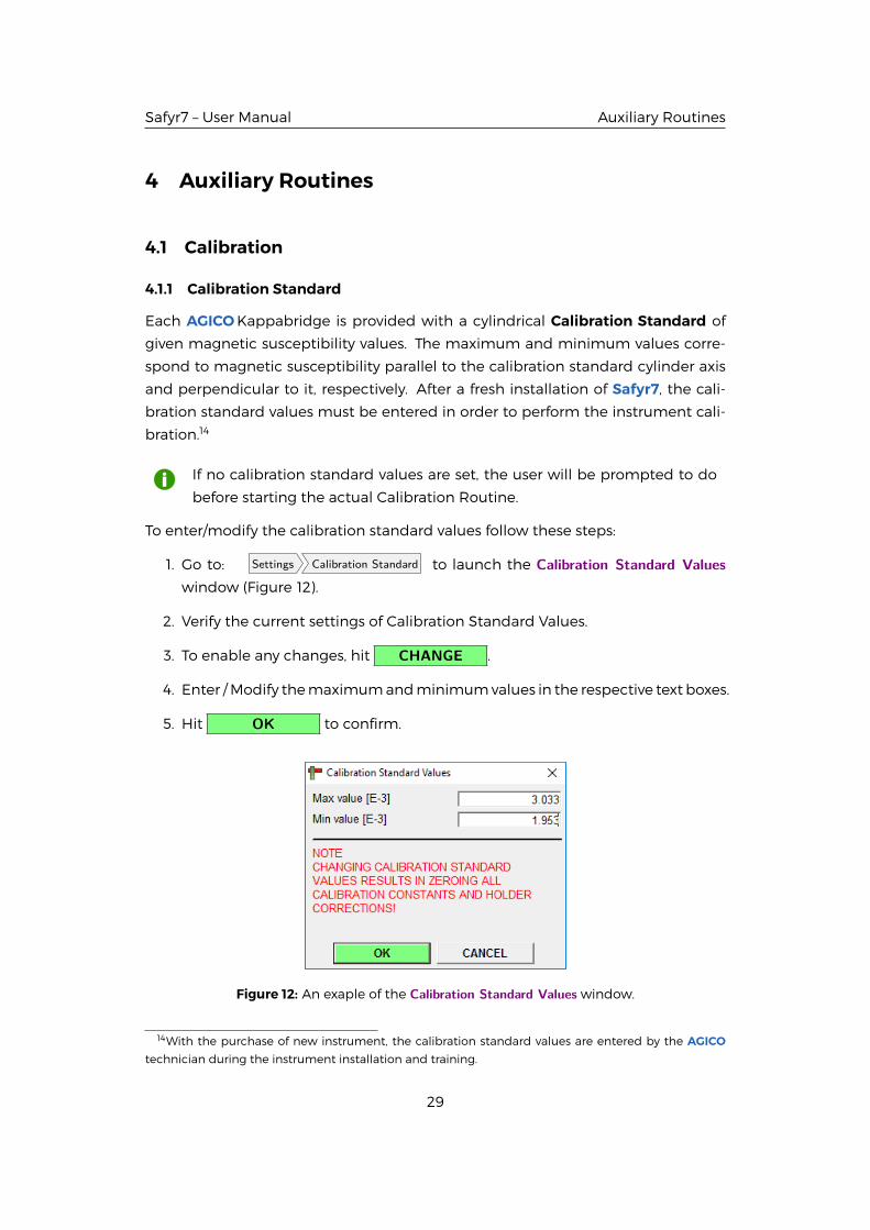
To enter/modify the calibration standard values follow these steps:
1. Go to: Settings Calibration Standard to launch the Calibration Standard Valueswindow (Figure 12).
2. Verify the current settings of Calibration Standard Values.
3. To enable any changes, hit CHANGE .
4. Enter /Modify themaximumandminimumvalues in the respective text boxes.
5. Hit OK to confirm.
Figure 12: An exaple of the Calibration Standard Values window.
14With the purchase of new instrument, the calibration standard values are entered by the AGICOtechnician during the instrument installation and training.
29
Safyr7 – User Manual Calibration
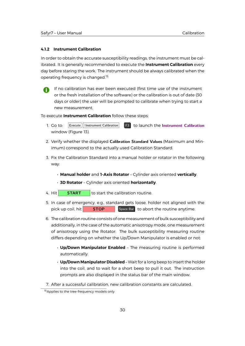
4.1.2 Instrument Calibration
In order to obtain the accurate susceptibility readings, the instrumentmust be cal-
ibrated. It is generally recommended to execute the Instrument Calibration every
day before staring the work. The instrument should be always calibrated when the
operating frequency is changed.15
If no calibration has ever been executed (first time use of the instrument
or the fresh installation of the software) or the calibration is out of date (30
days or older) the user will be prompted to calibrate when trying to start a
new measurement.
To execute Instrument Calibration follow these steps:
1. Go to: Execute Instrument Calibration F3 to launch the Instrument Calibrationwindow (Figure 13).
2. Verify whether the displayed Calibration Standard Values (Maximum and Min-
imum) correspond to the actually used Calibration Standard.
3. Fix the Calibration Standard into a manual holder or rotator in the following
way:
• Manual holder and 1-Axis Rotator – Cylinder axis oriented vertically.
• 3D Rotator – Cylinder axis oriented horizontally.
4. Hit START to start the calibration routine.
5. In case of emergency, e.g., standard gets loose, holder not aligned with the
pick up coil, hit STOP Space Bar to abort the routine anytime.
6. The calibration routine consists of onemeasurement of bulk susceptibility and
additionally, in the case of the automatic anisotropymode, onemeasurement
of anisotropy using the Rotator. The bulk susceptibility measuring routine
differs depending on whether the Up/Down Manipulator is enabled or not:
• Up/Down Manipulator Enabled – The measuring routine is performed
automatically.
• Up/DownManipulatorDisabled –Wait for a longbeep to insert theholder
into the coil, and to wait for a short beep to pull it out. The instruction
prompts are also displayed in the status bar of the main window.
7. After a successful calibration, new calibration constants are calculated.15Applies to the tree-frequency models only.
30
Safyr7 – User Manual Calibration
8. Hit SAVE to save and use the new calibration constants. Please
note that all previous holder correction values will be zeroed.
a)
b)
c)
Figure 13: Typical examples of the Instrument Calibration windows for a) Manual measur-
ingmodes (includingManual AnisotropyMode), b) 1-Axis Rotator, c) 3DRotator. (Results
for KLY5)
If Up/Down Manipulator is disabled, make sure that the plastic cylinder isinstalled into the coil.
31
Safyr7 – User Manual Holder Correction
Please note that for the purpose of the calibration routine, the field inten-
sity is switched to the instrument default value. When finished, the field
intensity is reset back to its original value.
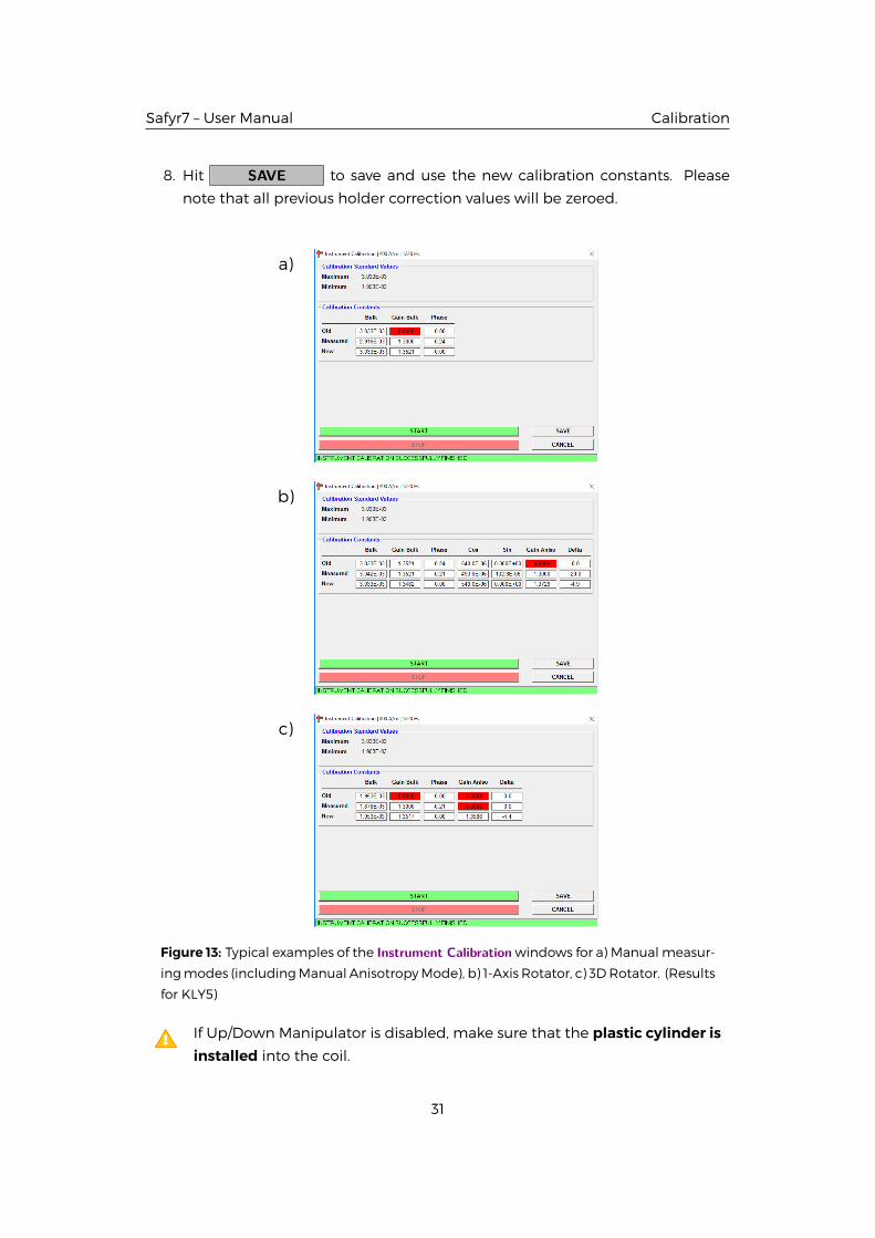
4.2 Holder Correction
The Holder Correction is intended to correct the measured susceptibility (aniso-
tropy) values for the susceptibility (anisotropy) of an empty holder (rotator).
If no holder correction has ever been executed (first-time use of the in-
strument or the fresh installation of the software) or the holder correction
values are suspicious, the user will be prompted to perform the holder cor-
rection routine when trying to start a new measurement.
It is recommended to perform the holder correction routine each time af-
ter instrument activation, change of operating frequency, change of holder
type, or change ofmeasuringmode (which usually implies different holder
type to be used).
To execute Holder Correction follow these steps:
1. Go to: Execute Holder Correction F4 to launch the Holder Correction window
(Figure 14).
2. Make sure that the holder or rotator is clean and empty (without any speci-
men or calibration standard).
3. Hit START to start the holder correction routine.
4. In case of emergency, hit STOP Space Bar to abort the routine any-
time.
5. The holder correction routine consists of three consecutive measurements of
bulk susceptibility and additionally, in the case of the automatic anisotropy
mode, three consecutive measurements of anisotropy using the Rotator. The
bulk susceptibility measuring routine differs depending on whether the U/D
Manipulator is enabled or not:
• Up/Down Manipulator Enabled – The measuring routine is performed
automatically.
• Up/DownManipulatorDisabled –Wait for a longbeep to insert theholder
into the coil, and to wait for a short beep to pull it out. The instruction
prompts are also displayed in the status bar of the main window.
32
Safyr7 – User Manual Holder Correction
a)
b)
c)
Figure 14: Typical examples of the Holder Correction windows for a) Manual measuring
modes (including Manual Anisotropy Mode), b) 1-Axis Rotator, c) 3D Rotator.
33
Safyr7 – User Manual Auxiliary Commands
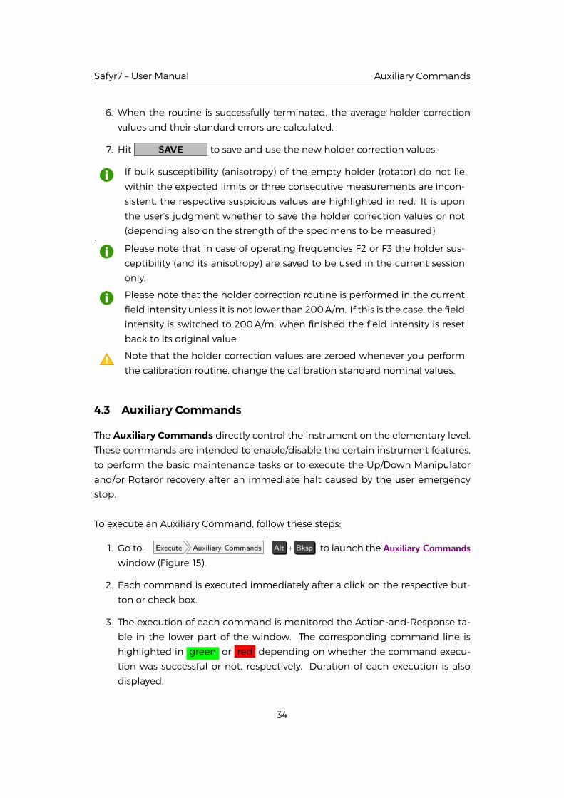
6. When the routine is successfully terminated, the average holder correction
values and their standard errors are calculated.
7. Hit SAVE to save and use the new holder correction values.
If bulk susceptibility (anisotropy) of the empty holder (rotator) do not lie
within the expected limits or three consecutive measurements are incon-
sistent, the respective suspicious values are highlighted in red. It is upon
the user’s judgment whether to save the holder correction values or not
(depending also on the strength of the specimens to be measured).
Please note that in case of operating frequencies F2 or F3 the holder sus-
ceptibility (and its anisotropy) are saved to be used in the current session
only.
Please note that the holder correction routine is performed in the current
field intensity unless it is not lower than 200A/m. If this is the case, the field
intensity is switched to 200A/m; when finished the field intensity is reset
back to its original value.
Note that the holder correction values are zeroed whenever you perform
the calibration routine, change the calibration standard nominal values.
4.3 Auxiliary Commands
The Auxiliary Commands directly control the instrument on the elementary level.
These commands are intended to enable/disable the certain instrument features,
to perform the basic maintenance tasks or to execute the Up/Down Manipulator
and/or Rotaror recovery after an immediate halt caused by the user emergency
stop.
To execute an Auxiliary Command, follow these steps:
1. Go to: Execute Auxiliary Commands Alt + Bksp to launch the Auxiliary Commandswindow (Figure 15).
2. Each command is executed immediately after a click on the respective but-
ton or check box.
3. The execution of each command is monitored the Action-and-Response ta-
ble in the lower part of the window. The corresponding command line is
highlighted in green or red depending on whether the command execu-
tion was successful or not, respectively. Duration of each execution is also
displayed.
34
Safyr7 – User Manual Auxiliary Commands
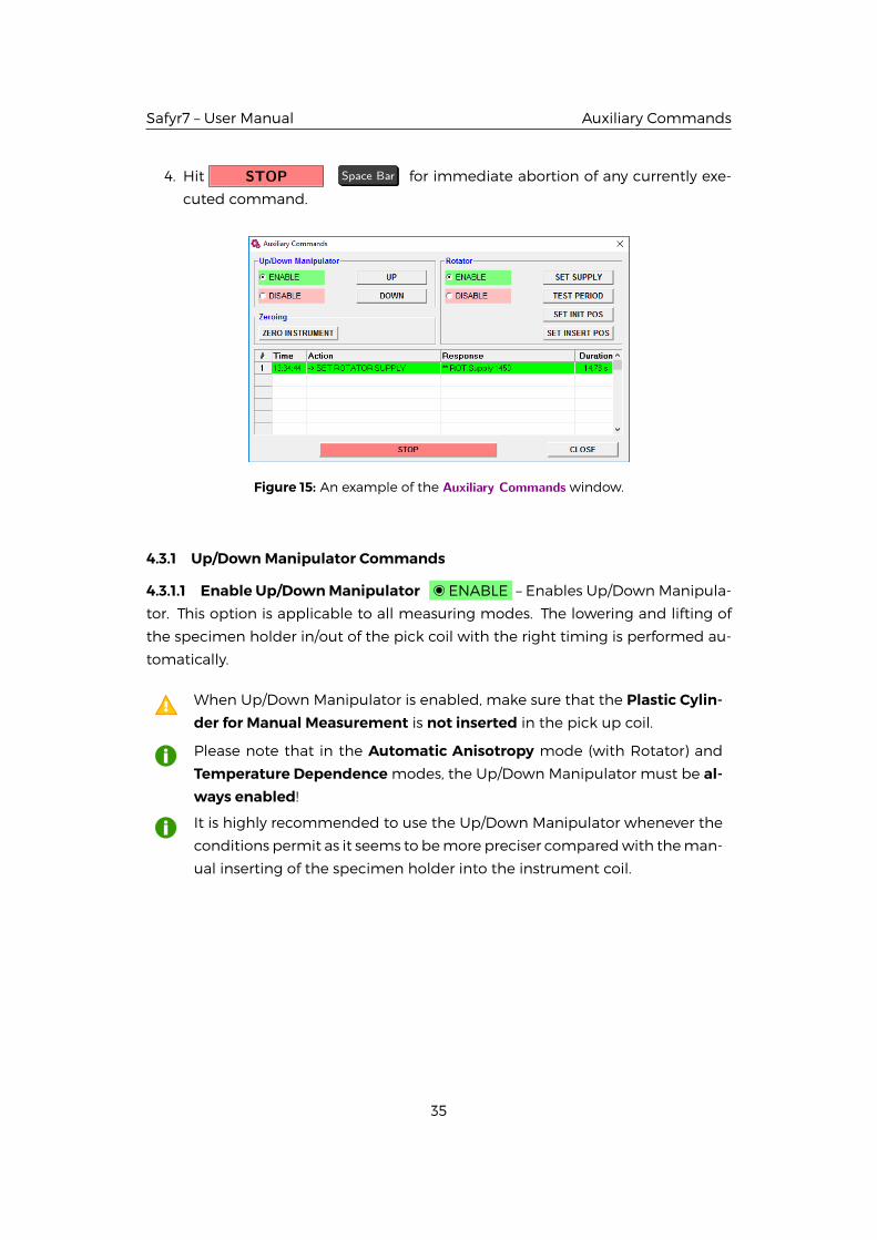
4. Hit STOP Space Bar for immediate abortion of any currently exe-
cuted command.
Figure 15: An example of the Auxiliary Commands window.
4.3.1 Up/Down Manipulator Commands
4.3.1.1 Enable Up/DownManipulator ENABLE – Enables Up/Down Manipula-
tor. This option is applicable to all measuring modes. The lowering and lifting of
the specimen holder in/out of the pick coil with the right timing is performed au-
tomatically.
When Up/Down Manipulator is enabled, make sure that the Plastic Cylin-der for Manual Measurement is not inserted in the pick up coil.
Please note that in the Automatic Anisotropy mode (with Rotator) and
Temperature Dependence modes, the Up/Down Manipulator must be al-ways enabled!
It is highly recommended to use the Up/Down Manipulator whenever the
conditions permit as it seems to bemore preciser comparedwith theman-
ual inserting of the specimen holder into the instrument coil.
35

Safyr7 – User Manual Auxiliary Commands
4.3.1.2 Disable Up/DownManipulator DISABLE – Disables Up/Down Manipu-
lator. This option is applicable only to the Individual Measurements, Field Depen-
dence andManual Anisotropymodes. When theUp/DownManipulator is disabled,
the specimen holder motions must be performed manually. To follow the right
timing, the user is guided by two acoustic signals (beeps) and the corresponding
[TEXT PROMPTS] in the status bar of the main Safyr7window:
1. Long Beep [SPECIMEN IN] – Insert the specimen into the pick up coil.
2. Short Beep [SPECIMEN OUT] – Pull the specimen out from the pick up coil.
When Up/Down Manipulator is disabled, the Plastic Cylinder for ManualMeasurement must be installed into the pick up coil to ensure the speci-
men is placed in its homogenous field area (central part).
4.3.1.3 Up / Down Commands The Up/Down Manipulator motions are executed
by pressing the respective buttons:
• UP – Moves Up/Down Manipulator to its upper position.
• DOWN – Moves Up/Down Manipulator to its lower position.
Duration of each movement is displayed in the Action-and-Response line. The Up
movement usually takes longer than theDownmovement but it should not exceed
3.6 s.
4.3.2 Rotator Commands
4.3.2.1 Enable / Disable Rotator Enabling or Disabling the Rotator can be per-
fomed by clicking on the respective check boxes:
• ENABLE – Enables the Rotator
• DISABLE – Disables the Rotator
4.3.2.2 Rotator Control Commands The following commands are related to the
spinning motion of the 3D or 1-Axis Rotator:
• SET SUPPLY – Gradually increases the voltage powering the rotator
in order to achieve the predefined speed of rotation. The final voltage dis-
played in the Action-and-Response line should be 1200–1400 [A/D convertor
units].
36

Safyr7 – User Manual Auxiliary Commands
• TEST PERIOD – Verifies the rotator speed and displays its rotational
period. The common values, depending on the firmware version of the in-
strument, are close to 2500ms or 2750ms.
• SET INIT POS – Spins the rotator until its initial position is set.
• SET INSERT POS – Turns the rotator about 10◦ clockwise in order that the
user is able to access the specimen fixing screw. This option applies to the 3D
Rotator only.
4.3.3 Zeroing Command
ZERO INSTRUMENT – Executes the zeroing routine of the pick up coils in order
to check the zeroing capability of the instrument. Duration of zeroing is usually
between 2–3 s.
37
Safyr7 – User Manual Sigma Test
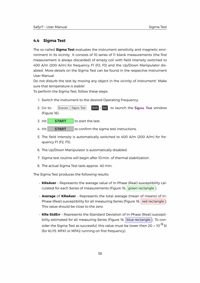
4.4 Sigma Test
The so-called Sigma Test evaluates the instrument sensitivity and magnetic envi-
ronment in its vicinity. It consists of 10 series of 11 blank measurements (the first
measurement is always discarded) of empty coil with field intensity switched to
400 A/m (200 A/m) for frequency F1 (F2, F3) and the Up/Down Manipulator dis-
abled. More details on the Sigma Test can be found in the respective Instrument
User Manual.
Do not disturb the test by moving any object in the vicinity of instrument! Make
sure that temperature is stable!
To perform the Sigma Test, follow these steps:
1. Switch the instrument to the desired Operating Frequency.
2. Go to: Execute Sigma Test Shift + Del to launch the Sigma Test window
(Figure 16).
3. Hit START to start the test.
4. Hit START to confirm the sigma test instructions.
5. The field Intensity is automatically switched to 400 A/m (200 A/m) for fre-
quency F1 (F2, F3).
6. The Up/Down Manipulator is automatically disabled.
7. Sigma test routine will begin after 10min. of thermal stabilization.
8. The actual Sigma Test lasts approx. 40 min.
The Sigma Test produces the following results:
• KReAver – Represents the average value of In-Phase (Real) susceptibility cal-
culated for each Series of measurements (Figure 16, green rectangle ).
• Average of KReAver – Represents the total average (mean of means) of In-
Phase (Real) susceptibility for all measuring Series (Figure 16, red rectangle ).
This value should be close to the zero.
• KRe StdErr – Represents the Standard Deviation of In-Phase (Real) suscepti-
bility estimated for all measuring Series (Figure 16, blue rectangle ). To con-
sider the Sigma Test as successful, this value must be lower then 20× 10-9 SI
(for KLY5, MFK1 or MFK2 running on first frequency).
38
Safyr7 – User Manual Sigma Test
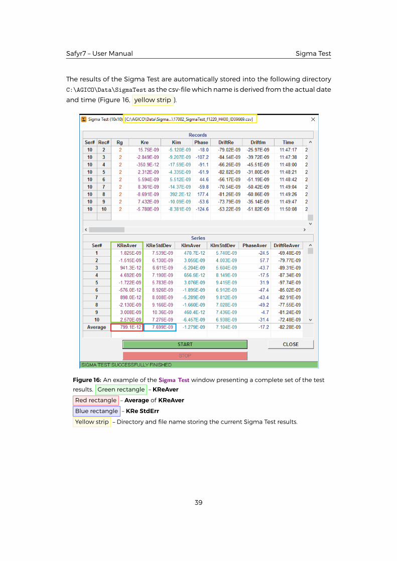
The results of the Sigma Test are automatically stored into the following directory
C:\AGICO\Data\SigmaTest as the csv-filewhich name is derived from the actual date
and time (Figure 16, yellow strip ).
Figure 16: An example of the Sigma Test window presenting a complete set of the test
results. Green rectangle – KReAver
Red rectangle – Average of KReAver
Blue rectangle – KRe StdErr
Yellow strip – Directory and file name storing the current Sigma Test results.
39

Safyr7 – User Manual Instrument Control
5 Instrument Control
As already described in details in the Settings Chapter (Page 10), Safyr7may work
in several different measuring modes. The measuring mode can be set in the In-strument Settings window ( Settings Instrument Settings F12 ), see Section 3.1.1, Page 11.
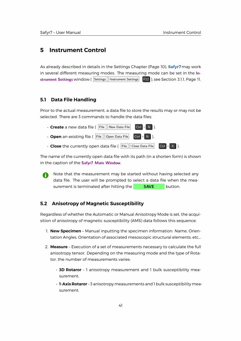
5.1 Data File Handling
Prior to the actual measurement, a data file to store the results may or may not be
selected. There are 3 commands to handle the data files:
• Create a new data file ( File New Data File Ctrl + N ).
• Open an existing file ( File Open Data File Ctrl + N ).
• Close the currently open data file ( File Close Data File Ctrl + X ).
The name of the currently open data file with its path (in a shorten form) is shown
in the caption of the Safyr7 Main Window.
Note that the measurement may be started without having selected any
data file. The user will be prompted to select a data file when the mea-
surement is terminated after hitting the SAVE button.
5.2 Anisotropy of Magnetic Susceptibility
Regardless of whether the Automatic or Manual Anisotropy Mode is set, the acqui-
sition of anisotropy of magnetic susceptibility (AMS) data follows this sequence:
1. New Specimen – Manual inputting the specimen information: Name, Orien-
tation Angles, Orientation of associatedmesoscopic structural elements, etc...
2. Measure – Execution of a set of measurements necessary to calculate the full
anisotropy tensor. Depending on the measuring mode and the type of Rota-
tor, the number of measurements varies:
• 3D Rotaror – 1 anisotropy measurement and 1 bulk susceptibility mea-
surement.
• 1-AxisRotaror – 3 anisotropymeasurements and 1 bulk susceptibilitymea-
surement.
41
Safyr7 – User Manual Anisotropy of Magnetic Susceptibility
• Manual Mode – 15 directional susceptibility measurements.
3. Calculate – Calculation of the results anddisplaying them in the user interface.
4. Save – Saving the results into data file(s) or, alternatively, Deleting (Canceling)
results.
5.2.1 New Specimen
To start a measuring sequence, follow these steps:
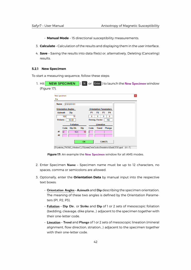
1. Hit NEW SPECIMEN ( N or Enter ) to launch theNew Specimenwindow
(Figure 17).
Figure 17: An example the New Specimen window for all AMS modes.
2. Enter Specimen Name – Specimen name must be up to 12 characters, no
spaces, comma or semicolons are allowed.
3. Optionally, enter the Orientation Data by manual input into the respective
text boxes:
• Orientation Angles –Azimuth andDipdescribing the specimenorientation.
The meaning of these two angles is defined by the Orientation Parame-
ters (P1, P2, P3).
• Foliation – Dip Dir. or Strike and Dip of 1 or 2 sets of mesoscopic foliation
(bedding, cleavage, dike plane...) adjacent to the specimen together with
their one-letter code.
• Lineation – Trend and Plunge of 1 or 2 sets of mesoscopic lineation (mineral
alignment, flow direction, striation...) adjacent to the specimen together
with their one-letter code.
42
Safyr7 – User Manual Anisotropy of Magnetic Susceptibility
4. As an alternative to the manual input of Orientation Data, one may use a Ge-ological File (ged-file) where the specimen information is stored:
(a) Open a desired ged-file: File Open ( Ctrl + G ).
(b) List of sample names stored in this ged-file is displayed on the right-hand
site of the New Specimen window (Figure 17).
(c) To copy the specimen information from the ged-file to the respective textboxes, click on the desired sample name or type the specimen name di-rectly into the Name text box.Note that the specimen name typed in the Name text box may be longer (may include suf-
fices or indexes) than that stored in the ged-file. This way, onemay use the same orientation
data formultiple specimens having originated from the same sample (cubic specimens cut
from an oriented hand sample, cylindrical specimens cut from an oriented core sample).
For example, S1 is a sample name stored in the ged-file while S1-1, S1/2, S1-A, S1B3 are various
specimens having originated from that sample and thus having the same orientation.
5. Hit OK ( Enter ) to finish. The New Specimen window closes and
the specimen information is copied into the Specimen Info Frame of the
Safyr7 Main Window (Figure 18, 19, 20).
Use the Tab key to move among multiple text boxes.
5.2.2 Anisotropy Measurements
5.2.2.1 3D Rotator The Safyr7 Main Window for the Automatic Anisotropy Mea-
surement with 3D Rotator is shown in the Figure 18. The measuring routine is very
easy and consists of the following steps:
1. Fix the specimen into the Rotator using the screw on the right hand side of
the Rotator (Figure 31).
2. Hit ANISO ( F1 or Enter ) to start the anisotropy measurement.
The measuring procedure is fully automatic:
(a) Rotator moves down into the coil.
(b) The instrument is zeroed.
(c) The specimen starts spinning and a set of Deviatoric susceptibilities is
measured.
(d) Rotator moves up from the coil.
3. Hit BULK ( F2 or Enter ) to start the bulk susceptibility measure-
ment. With the �DAuto BULK option being checked (default state), the bulk
susceptibility measurement starts automatically when the anisotropy mea-
surement is finished. The measuring procedure is fully automatic:
43

Safyr7 – User Manual Anisotropy of Magnetic Susceptibility
(a) The instrument is zeroed.
(b) Rotator moves down into the coil.
(c) Bulk susceptibility is measured.
(d) Rotator moves up from the coil.
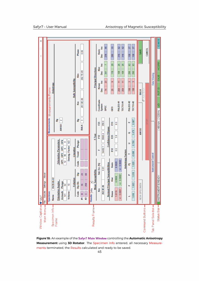
The measured values are presented in the Measurements Frame (Figure 18):
• Anisotropy
– Rg – Range of the anisotropy measurement (This reflects the magnitude
of deviatoric susceptibility).
• Bulk Susceptibility – Bulk susceptibility along the x-axis of the specimen
– Rg – Range of the bulk susceptibility measurement.
– Kre – Real (In-Phase) susceptibility.
– Kim – Imaginary (Out-of-Phase) susceptibility.
– Phase – Phase angle.
44
Safyr7 – User Manual Anisotropy of Magnetic Susceptibility
Figure 18: An example of the Safyr7 Main Window controlling theAutomaticAnisotropy
Measurement using 3D Rotator: The Specimen Info entered, all necessary Measure-
ments terminated, the Results calculated and ready to be saved.45
Safyr7 – User Manual Anisotropy of Magnetic Susceptibility
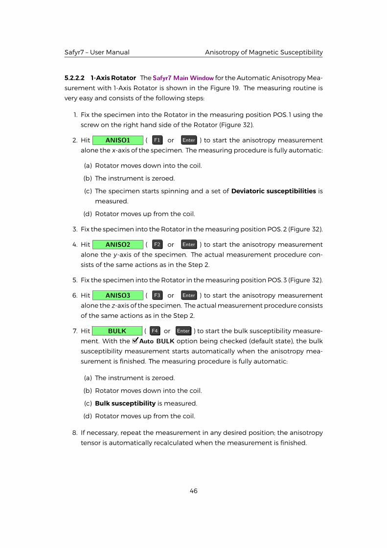
5.2.2.2 1-AxisRotator The Safyr7 Main Window for the Automatic AnisotropyMea-
surement with 1-Axis Rotator is shown in the Figure 19. The measuring routine is
very easy and consists of the following steps:
1. Fix the specimen into the Rotator in the measuring position POS. 1 using the
screw on the right hand side of the Rotator (Figure 32).
2. Hit ANISO1 ( F1 or Enter ) to start the anisotropy measurement
alone the x-axis of the specimen. Themeasuring procedure is fully automatic:
(a) Rotator moves down into the coil.
(b) The instrument is zeroed.
(c) The specimen starts spinning and a set of Deviatoric susceptibilities is
measured.
(d) Rotator moves up from the coil.
3. Fix the specimen into theRotator in themeasuring position POS. 2 (Figure 32).
4. Hit ANISO2 ( F2 or Enter ) to start the anisotropy measurement
alone the y-axis of the specimen. The actual measurement procedure con-
sists of the same actions as in the Step 2.
5. Fix the specimen into the Rotator in themeasuring position POS. 3 (Figure 32).
6. Hit ANISO3 ( F3 or Enter ) to start the anisotropy measurement
alone the z-axis of the specimen. The actualmeasurement procedure consists
of the same actions as in the Step 2.
7. Hit BULK ( F4 or Enter ) to start the bulk susceptibility measure-
ment. With the �DAuto BULK option being checked (default state), the bulk
susceptibility measurement starts automatically when the anisotropy mea-
surement is finished. The measuring procedure is fully automatic:
(a) The instrument is zeroed.
(b) Rotator moves down into the coil.
(c) Bulk susceptibility is measured.
(d) Rotator moves up from the coil.
8. If necessary, repeat the measurement in any desired position; the anisotropy
tensor is automatically recalculated when the measurement is finished.
46
Safyr7 – User Manual Anisotropy of Magnetic Susceptibility
The measured values are presented in the Measurements Frame (Figure 19):
• Anisotropy – Anisotropy curve for each spinning plane.
– Rg – Range of the anisotropy measurement (This reflects the magnitude
of deviatoric susceptibility).
– Cos – Cosine component of the average anisotropy curve.
– Sin – Sine component of the average anisotropy curve.
– Amp – Amplitude of the average anisotropy curve.
– Error – Standard deviation of the individual curves from the average curve.
– Error [%] – Standard deviation divided by the amplitude value.
The error for each of anisotropy curve is standard deviation of the individual curves (there are two
sine wave curves for one physical revolution) from the average curve and the error [%] gives this
deviation divided by the amplitude value. This error has only informative meaning and reflects
the ratio between the noise and ’anisotropy’ signal for measurement in one plane only. Thus it
depends not only on absolute susceptibility of the specimenmeasured butmainly on the degree
of anisotropy in an individual plane perpendicular to the axis of rotation. In case there is no
anisotropy in one of the three planes this error may be over 100% and has no physical meaning.
In case the anisotropy in one plane has ’reasonable’ value, the usual value is lower 5%, but it does
not reflect the quality of the measurement, but also the level of anisotropy in one plane.
• Bulk Susceptibility – Bulk susceptibility along the x-axis of the specimen
– Rg – Range of the bulk susceptibility measurement.
– Kre – Real (In-Phase) susceptibility.
– Kim – Imaginary (Out-of-Phase) susceptibility.
– Phase – Phase angle.
47
Safyr7 – User Manual Anisotropy of Magnetic Susceptibility
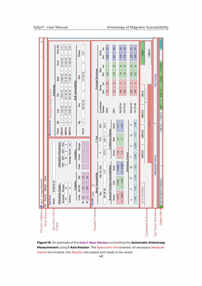
Figure 19: An example of the Safyr7 Main Window controlling theAutomaticAnisotropy
Measurement using 1-Axis Rotator: The Specimen Info entered, all necessary Measure-
ments terminated, the Results calculated and ready to be saved.48

Safyr7 – User Manual Anisotropy of Magnetic Susceptibility
5.2.2.3 Manual Mode The Safyr7 Main Window for the Manual Anisotropy Mea-
surement is shown in the Figure 20. The measuring routine consists of the follow-
ing steps:
1. Fix the specimen into the specimen holder in the measuring position POS. 1
(Figure 33, 34).
2. Hit BULK P1 ( Enter ) to start the directional susceptibility measure-
ment in Pos. 1. The measuring procedure depends on whether the Up/Down
Manipulator (U/D) is Enabled or Disabled:
(a) The instrument is zeroed.
(b) • U/D Enabled: Holder moves down into the pick up coil.
• U/D Disabled: Long Beep (Status Bar Prompt: SPECIMEN IN) indi-
cates to insert the holder into the pick up coil.
(c) Bulk susceptibility is measured.
(d) • U/D Enabled: Holder moves up from the pick up coil.
• U/D Disabled: Short Beep (SPECIMEN OUT) indicates to pull the
holder out from the pick up coil.
3. The respective directional susceptibilitymeasurement is displayed in theMea-
surements Frame.
4. With the�DAuto NEXT option being checked (default state), the BULK PXbutton is automatically set to measure the next position. Alternatively, click
on PREV POS or NEXT POS to manually set the previous or next
position, respectively. These commands are particularly usefulwhenoneneeds
to re-measure some position(s).
5. Fix the specimen into the holder in the measuring position POS. 2 (Figure 33,
34).
6. Hit BULK P2 ( Enter ) to start the directional susceptibility measure-
ment in Pos. 2. The measuring procedure follows the same actions as in Step
2.
7. Continue until all 15 directional susceptibilities are measured.
8. If necessary, repeat the measurement in any desired position; the anisotropy
tensor is automatically recalculated when the measurement is finished.
49
Safyr7 – User Manual Anisotropy of Magnetic Susceptibility
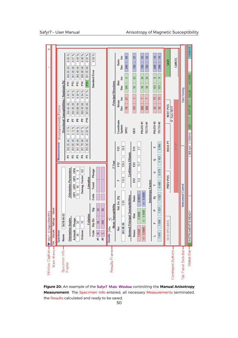
Figure 20: An example of the Safyr7 Main Window controlling the Manual Anisotropy
Measurement: The Specimen Info entered, all necessary Measurements terminated,
the Results calculated and ready to be saved.50
Safyr7 – User Manual Anisotropy of Magnetic Susceptibility
When all 15 directional susceptibilities are measured, the susceptibility tensor is
fitted using the least squares method and the errors are displayed next to each
directional susceptibility value in the Measurements Frame (Figure 20). The errors
of the fit are calculated as the deviation of the particular directional susceptibility
from the calculated anisotropy ellipsoid expressed in [%].
5.2.3 Tensor Calculations
Regardless of whether the Automatic or Manual Anisotropy Mode is used, the cal-
culation of the anisotropy tensor is performed automatically whenever all neces-
sary data are available. Various parameters derived from the anisotropy tensor are
displayed in the Results (Figure 18, 19, 20):
• Mean Susceptibility
– Km – Mean susceptibility [SI units].
– Std. Err – Standard error [%] of mean susceptibility.
• F-Test
– F – Statistics for anisotropy testing.
– F12 – Statistics for triaxiality testing.
– F23 – Statistics for uniaxiality testing.
• Normed Principal Susceptibilities – Principal susceptibilities normedby thenorm-
ing factor and errors in their determination.
• Confidence Ellipses – Confidence ellipses of determination of the principal sus-
ceptibility directions; they are expressed in a slightly different way depending
on the used measuring mode:
– 3D Rotator: E12, E23, E13 confidence angles (on the 95% probability level)
– 1-Axis Rotator: Semi-axes of the confidence ellipse for rotation axis Kmax,Kint, Kmin angles
– Manual measurements: E12, E23, E13 confidence angles (on the 95%
probability level)
• Anisotropy Factors – Values of the selected quantitative anisotropy factors as
defined in the anisotropy factor settings (see page28)
• Principal Directions – Orientations of principal susceptibility directions (Kmax,Kint, Kmin) expressed as declinations (Dec) and Inclination (Inc) in various Co-ordinate Systems:
51
Safyr7 – User Manual Anisotropy of Magnetic Susceptibility
– SPEC – Specimen Coordinate System.
– GEO – Geographic Coordinate System. Calculated only when the Orien-
tation Angles were entered.
– PALEO #1 – Paleogeographic Coordinate System #1. Calculated only
when the 1st (#1) mesoscopic fabric elements (Foliation and/or Lineation)
were entered.
– TECTO #1 – Tectonic Coordinate System #1. Calculated only when the
1st (#1) mesoscopic fabric elements (Foliation and/or Lineation) were en-
tered.
– PALEO #2 – Paleogeographic Coordinate System #2. Calculated only
when the 2nd (#2)mesoscopic fabric elements (Foliation and/or Lineation)
were entered.
– TECTO #2 – Tectonic Coordinate System #2. Calculated only when the
2nd (#2) mesoscopic fabric elements (Foliation and/or Lineation) were
entered.
To evaluate the quality of anisotropymeasurements, use the F-Test values and 95% confidence ellipses.
The general rule is as follows. If the F-Test values are high (> 5), the confidence ellipses are small and the
respective principal direction is well defined. The sensitivity of AMS measurement for the field inten-
sity 400A/m on MFK1 is 2× 10⁻⁸ [SI], the anisotropy of the specimens with mean susceptibility about
5× 10⁻⁶ [SI] can be measured, but the confidence ellipses may be in some cases larger, it depends on
type of anisotropy. The sensitivity is approximately linearly decreasing with decreasing field intensity.
Due to the influence of Rotator motor on the AMS measurement it may be problematic using it at op-
erating frequencies F2 and F3 in case of specimens weaker than 100× 10−6 SI units and with degree of
anisotropy lower than 5%. For this case at F3 it is recommended to use manual measurement method
in 15 directions to eliminate the influence of motor of the Rotator.
5.2.4 Saving Results
• Hit SAVE ( Enter or S ) to append the results as a new record
into the currently open data file.
OR
• Hit CANCEL ( Esc ) to delete the results without saving.
If no data file is open, the user is prompted to create a newdata file or open
an existing file after hitting SAVE .
To store the results into into other file than that currently open, close the
current data file prior hitting SAVE .
52

Safyr7 – User Manual Anisotropy of Magnetic Susceptibility
The anisotropy results are saved together with the mesoscopic fabric elements (fo-
liations and lineations) simultaneously into 3 types of files:
1. ams-file (FileName.ams) – Enhanced binary data file intended to be further
processed using AGICO Anisoft5 software (Ver. 5).
2. ran-file (FileName.ran) – Long-time standard binary data file intended to be
further processed using AGICOAnisoft4 software (Ver. 4 and higher).
3. asc-file (FileName.asc) – ASCII text file which serves as a log-file of each mea-
surement, not intended to be further processed.
The anisotropy results for multiple specimens (those contained in the currently
open data file) may be viewed in a graphical form in the Data Viewing tab panel of
the Safyr7 Main Window.
53
Safyr7 – User Manual Bulk Susceptibility
5.3 Bulk Susceptibility
Before starting the bulk susceptibility measurements, the user may set:
• Susceptibility Normalization (Volume / Mass-normalized) – See Section 3.2,
Page 25
• Field Intensity – See Section 3.1.2.1, Page 23
• Operating Frequency16 – See Section 3.1.3, Page 24
DONOT USE 3D ROTATOROR 1-AXIS ROTATOR to hold the specimen. It is
highly recommended to use the appropriate Specimen Holder or Vesselfor Fragments.
UP/DOWN MANIPULATOR can be optionally enabled/disabled in the Aux-ialiary Commands window.
5.3.1 Individual Measurements Mode
The Individual Measurements Mode controls a sequence of individual measure-
ments of volume/mass normalized susceptibility in desired field intensity and, if
applicable, in various operating frequencies17.
The Individual Measurements Mode can be set in the Instrument Settings window
( Settings Instrument Settings or F12 ), see Section 3.1.1.3, Page 13. The Safyr7 MainWindow for the Individual Measurements Mode is shown in Figure 22.
1. Fix the specimen into the Specimen Holder or Vessel for Fragments.
2. Hit NEW SPECIMEN ( N or Enter ) to launch theNew Specimenwindow
(Figure 21).
3. Fill the following text boxes:
• Name – Specimen name must be up to 12 characters, no spaces, comma
or semicolons are allowed.
• Volume / Mass – Actual Volume / Mass of the specimen. If no value is
entered, the default Volume / Mass will be used.
• Note – Optional note containing a further description of the specimen,
measuring conditions or so on.
16Applies only to the three-frequency instrument versions17Applies to be three-frequency versions only
54
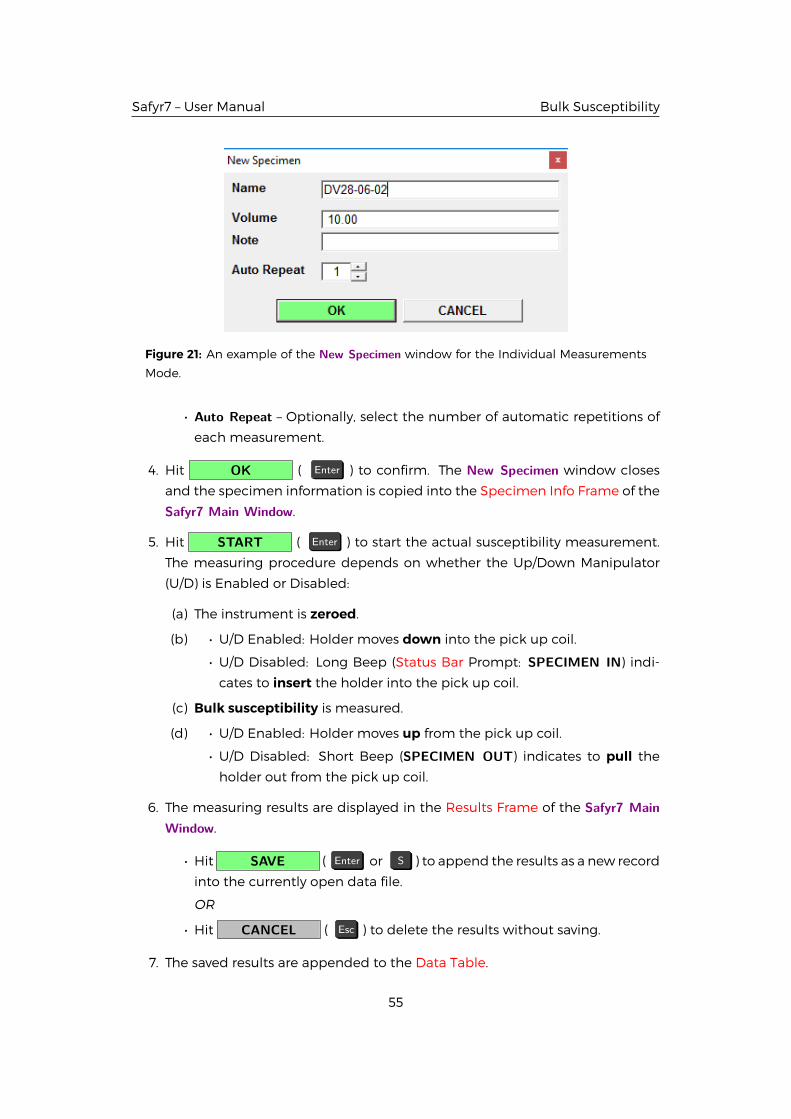
Safyr7 – User Manual Bulk Susceptibility
Figure 21: An example of the New Specimen window for the Individual Measurements
Mode.
• Auto Repeat – Optionally, select the number of automatic repetitions of
each measurement.
4. Hit OK ( Enter ) to confirm. The New Specimen window closes
and the specimen information is copied into the Specimen Info Frame of the
Safyr7 Main Window.
5. Hit START ( Enter ) to start the actual susceptibility measurement.
The measuring procedure depends on whether the Up/Down Manipulator
(U/D) is Enabled or Disabled:
(a) The instrument is zeroed.
(b) • U/D Enabled: Holder moves down into the pick up coil.
• U/D Disabled: Long Beep (Status Bar Prompt: SPECIMEN IN) indi-
cates to insert the holder into the pick up coil.
(c) Bulk susceptibility is measured.
(d) • U/D Enabled: Holder moves up from the pick up coil.
• U/D Disabled: Short Beep (SPECIMEN OUT) indicates to pull the
holder out from the pick up coil.
6. The measuring results are displayed in the Results Frame of the Safyr7 MainWindow.
• Hit SAVE ( Enter or S ) to append the results as a new record
into the currently open data file.
OR
• Hit CANCEL ( Esc ) to delete the results without saving.
7. The saved results are appended to the Data Table.
55
Safyr7 – User Manual Bulk Susceptibility
The individual susceptibility measurements are saved into a space-delimiter ASCII
text file with a fixed format – bulk-file (FileName.bulk). For a detailed description
of bulk-file format, see Section ?? in Appendix.
The individual susceptibility measurements (those contained in the currently open
data file) may be viewed and partially processed (e.g., calculation of frequency-
dependence parameters) in the Data Viewing panel of the Safyr7 Main Window.If no data file is open, the user is prompted to create a newdata file or open
an existing file after hitting SAVE .
To save the results into other file than that currently open, close the current
data file prior hitting SAVE .
Here are a few tips and recommendations for the measurements of the frequency-dependent suscep-
tibility:
1. After the change of the operating frequency the instrument pick up coils are disbalanced and
they require at least 10min to be stabilized. Thus it is not recommended to change the oper-
ating frequency too often. To investigate the frequency-dependent susceptibility of a group of
specimens, follow the recommended procedure:
(a) Set the first desired operating frequency and let the instrument to stabilize
(b) Perform the holder correction routine
(c) Measure all specimens of the group
(d) Set the second desired operating frequency and the instrument to stabilize
(e) Measure all specimens at the second frequency
2. The frequency-dependent susceptibility is calculated from two (three) independent susceptibility
measurements. As the calculation routine must combine these independent measurements, it
is essential to use exactly in the same name each time the same specimen ismeasured at various
operating frequencies.
3. To eliminate the possible effect of field dependence, the field intensity must be the same for
each operating frequency. For that reason, the default field intensity is automatically set when
the operating frequency is changed.
4. To avoid the possible anisotropy effects, the specimens must be orientated in the same way dur-
ing measurements at each operating frequency. In the case of the cylindrical specimens, it is
recommended to measure in vertical orientation so that the cylinder axis is parallel to the axis of
the instrument coil (Figure 30, Page 74). That way, magnetic susceptibility parallel to the cylin-
der axis regardless of the specimen orientation with respect to that axis; this cannot be exactly
reached in the perpendicular orientation due to the slight specimenmisorientations during each
individual measurements.
56
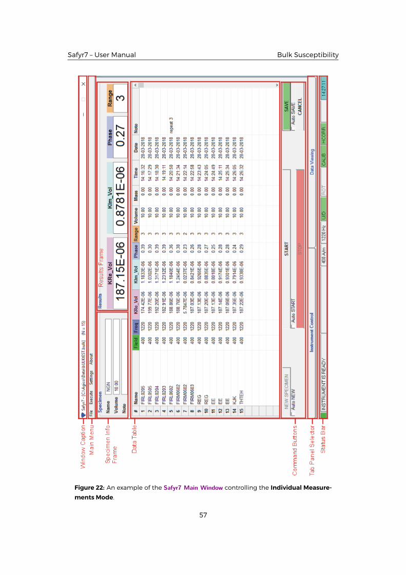
Safyr7 – User Manual Bulk Susceptibility
Figure 22: An example of the Safyr7 Main Window controlling the Individual Measure-
ments Mode.
57

Safyr7 – User Manual Bulk Susceptibility
5.3.2 Field Dependence Mode
The FieldDependenceMode controls the automatic acquisition of field-dependent
susceptibility curves (magnetic susceptibility as a function of field intensity) in a
preset sequence of field intensities. The results are presented as volume/mass nor-
malized in-phase and out-of-phase18 susceptibility both in tabular and graphical
form. The acquired field dependence data can be saved into the space-delimited
data files.
The FieldDependenceMode can be set in the Instrument Settings window ( Settings
Instrument Settings or F12 ), see Section 3.1.1.4, Page 14. The Safyr7 Main Window for
the Field Dependence Mode is shown in Figure 24.
To acquire a field-dependent susceptibility curve, follow these steps:
1. Fix the specimen into the Specimen Holder or Vessel for Fragments.
2. Open a data file. This step is only optional as the user is prompted to do so
each time the acquired curve is to be saved into disk (see Step 14).
3. Review thedesired field sequence in theData Table andhit FIELD SEQUENCEto launch the Field Dependence Settings window in order to modify the field
sequence and/or instrument ranging mode (see Section 3.1.2.1, Page 23).
4. Hit NEW SPECIMEN ( N or Enter ) to launch theNew Specimenwindow
(Figure 23).
Figure 23: An example of the New Specimen window for the Field Dependence Mode.
5. Fill the following text boxes:
• Name – Specimen name must be up to 12 characters, no spaces, comma
or semicolons are allowed.18Applies to the KLY5 models only.
58
Safyr7 – User Manual Bulk Susceptibility
• Volume / Mass – Actual Volume / Mass of the specimen. If no value is
entered, the default Volume / Mass will be used.
• Note – Optional note containing a further description of the specimen,
measuring conditions or so on.
6. Hit OK ( Enter ) to confirm. The New Specimen window is closed
and the specimen information is copied into the Specimen Info Frame of the
Safyr7 Main Window.
7. Hit START ( Enter ) to start the acquisition of field dependence curve.
(Hit STOP ( Space Bar ) to abort the curve acquisition in case of emer-
gency, e.g., specimen gets loose, holder not alignedwith the pick up coil...etc.)
8. The 1st field intensity in the desired field sequence is automatically set and
the instrument is shortly stabilized.
9. Magnetic susceptibility is measured. The actual measuring procedure de-
pends onwhether the Up/DownManipulator is Enabled or Disabled (see Sec-
tion 4.3.1, Page 36).:
(a) The instrument is zeroed.
(b) • U/D Enabled: Holder automaticallymovesdown into the pick up coil.
• U/D Disabled: Long Beep (Status Bar Prompt: SPECIMEN IN) indi-
cates to manually insert the holder into the pick up coil.
(c) Bulk susceptibility is measured.
(d) • U/D Enabled: Holder automatically moves up from the pick up coil.
• U/D Disabled: Short Beep (SPECIMEN OUT) indicates to manually
pull the holder out from the pick up coil.
10. The currently measured susceptibility values are appended to the Data Table
and the Field-dependence Plot is continuously re-drawn. In addition, several
Field-dependence Indexes are calculated and displayed (Figure 24).
11. The steps 8, 9, and 10 are repeated until the susceptibility is measured in all
fields in the desired field sequence.
12. The original field intensity is automatically reset.
13. The field dependence curve is terminated and a message box displaying ter-
mination time and measurement duration appears. Optionally, when se-
lected, a ring tone sounds.
59

Safyr7 – User Manual Bulk Susceptibility
14. • Hit SAVE ( Enter or S ) to append the measured curve as
a set of new records into a data file. In order to enable saving each curve
into a separate file, the Save Data dialog is automatically launched and
the user may select a new files name (the current data file is offered as a
default option).
OR
• Hit CANCEL ( Esc ) to delete the results without saving.
To save the results into other file than that currently open, close the current
data file prior hitting SAVE .
The field dependence curves are saved into a space-delimiter ASCII text file with a
fixed format – bulk-file (FileName.bulk). Each curve may be saved into a separate
bulk-file or one bulk-file may contain multiple curves.
The field dependence curves for multiple specimens (those contained in the cur-
rently open data file) may be viewed in the Data Viewing panel of the Safyr7 MainWindow.
As the curve acquisition is a lasting process, the measured
data are automatically appended into a temporary data file:
C:\Agico\Data\TemporaryData\SpecimenName.bulk. This file may be useful
to recover the data in case that the data acquisition is forcefully aborted
(software crash, power blackout...etc.).
60
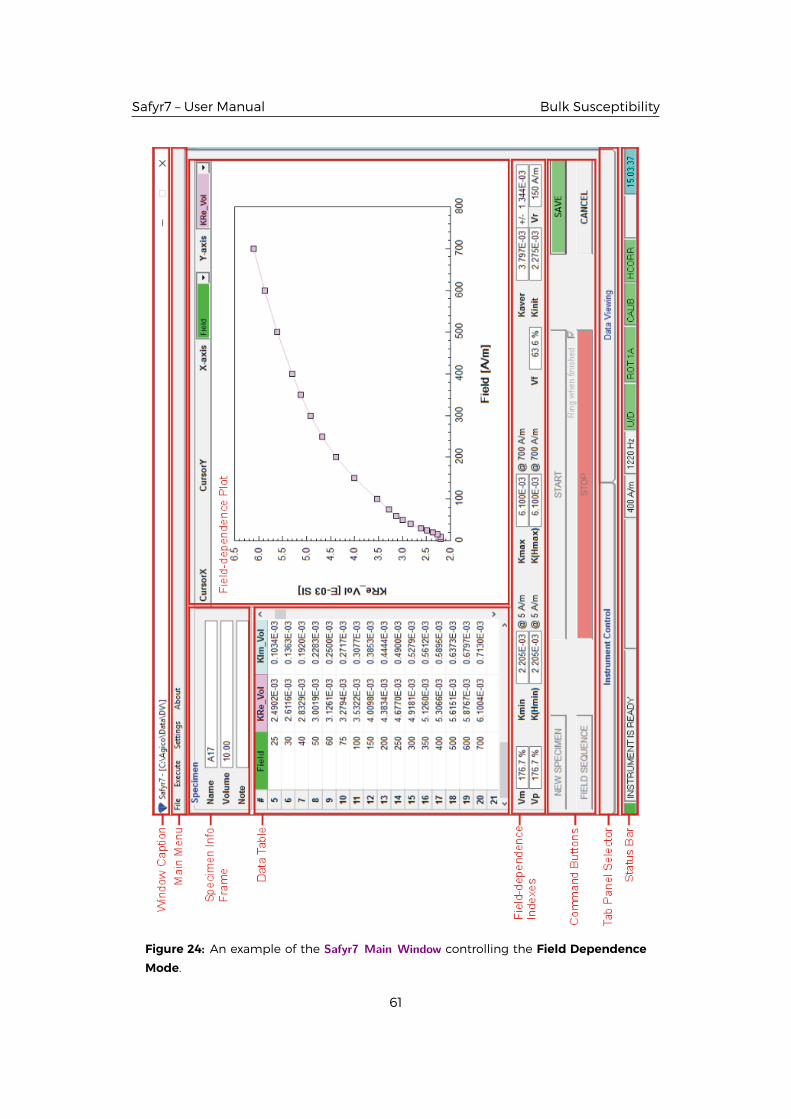
Safyr7 – User Manual Bulk Susceptibility
Figure 24: An example of the Safyr7 Main Window controlling the Field Dependence
Mode.
61
Safyr7 – User Manual Bulk Susceptibility
Field variation indexes are defined as follows:
• Vm index characterizes the maximum susceptibility variation with field
Vm = 100kmax − kmin
kmin[%]
where kmax and kmin are the maximum and minimum susceptibilities, respectively, measured
during onemeasuring run. The field intensities inwhichminimumandmaximumsusceptibilities
were measured are presented in parenthesis.
• Vp index characterizes the variation of susceptibility between the weakest and strongest mea-
suring field
Vp = 100kHmax − kHmin
kHmin[%]
where kHmax and kHmin are the susceptibilitiesmeasured atmaximumandminimumfield inten-
sities, respectively. Interval of field intensities used for the calculation is presented in parenthesis.
• Va index. As the susceptibilitiesmeasured at the very low fieldsmay be affected by relatively large
errors inweaklymagnetic specimens, it is useful to introduce an indexwhich eliminates the effect
of the errors at least partially, because the errors are distributed approximately randomly
Va = 100kHmax − ki
ki[%]
where ki is the average susceptibilitymeasured at the field intensities Hpeak = 15A/mand kHmax is
the susceptibility measured at themaximum field. Average susceptibility at the beginning of the
k(H) curve, Ki is presented. The interval of field intensities used for the calculation in presented
in parenthesis.
• Vf index. The susceptibility vs. field data usually very well fit the straight line in some range of
fields. In this case it is useful to use an index that is calculated from the fit straight line
Vf = 100ku − kl
kl[%]
where kl and ku are the susceptibilities calculated from the fit straight line at the beginning and
at the end of the field range considered, respectively. The field intensities of the beginning and
at the end of the straight line are presented in parenthesis.
• Vr index gives the upper limit of the validity of the Rayleigh law. It is calculated as follows. A
straight line is fit to the susceptibility vs. field data in the field range between 10A/m and 80A/m.
The lower limit of this range is high enough to avoid very low fields in which the measuring error
may be high for many specimens, and the upper limit is low enough to respect the validity of the
Rayleigh law in themost specimens. Using this straight line, theoretical Rayleigh law susceptibil-
ities are calculated successively also for stronger fields. The index Vr equals the maximum field
in which the measured susceptibility deviates from the theoretical one less than 5%.
In addition the initial susceptibility, Kint, is calculated as the intercept of the above straight line
with the ordinate.
In addition to the above-described indexes, the minimum, Kmin, the maximum, Kmax, and the average
susceptibilities, Kaver, (together with the standard error) are presented.
62
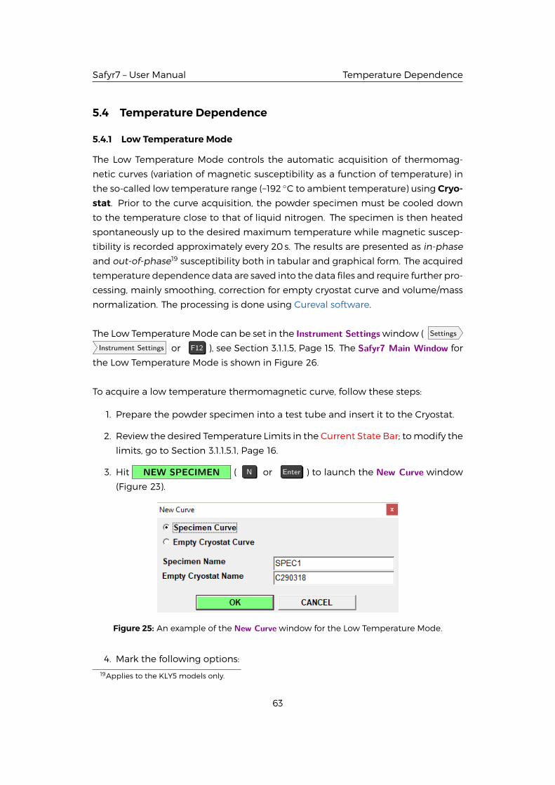
Safyr7 – User Manual Temperature Dependence
5.4 Temperature Dependence
5.4.1 Low Temperature Mode
The Low Temperature Mode controls the automatic acquisition of thermomag-
netic curves (variation of magnetic susceptibility as a function of temperature) in
the so-called low temperature range (−192 ◦C to ambient temperature) using Cryo-stat. Prior to the curve acquisition, the powder specimen must be cooled down
to the temperature close to that of liquid nitrogen. The specimen is then heated
spontaneously up to the desired maximum temperature while magnetic suscep-
tibility is recorded approximately every 20 s. The results are presented as in-phase
and out-of-phase19 susceptibility both in tabular and graphical form. The acquired
temperature dependence data are saved into the data files and require further pro-
cessing, mainly smoothing, correction for empty cryostat curve and volume/mass
normalization. The processing is done using Cureval software.
The Low Temperature Mode can be set in the Instrument Settings window ( Settings
Instrument Settings or F12 ), see Section 3.1.1.5, Page 15. The Safyr7 Main Window for
the Low Temperature Mode is shown in Figure 26.
To acquire a low temperature thermomagnetic curve, follow these steps:
1. Prepare the powder specimen into a test tube and insert it to the Cryostat.
2. Review the desired Temperature Limits in the Current State Bar; tomodify the
limits, go to Section 3.1.1.5.1, Page 16.
3. Hit NEW SPECIMEN ( N or Enter ) to launch the New Curve window
(Figure 23).
Figure 25: An example of the New Curve window for the Low Temperature Mode.
4. Mark the following options:19Applies to the KLY5 models only.
63
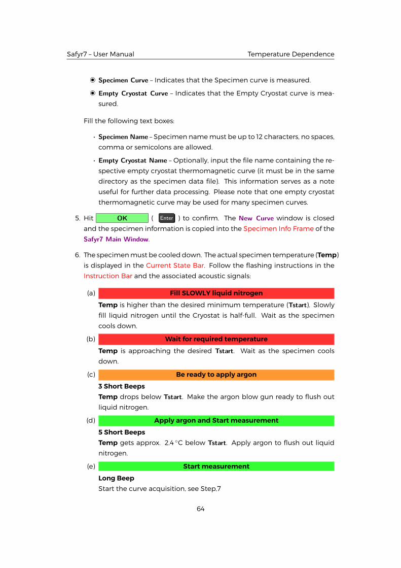
Safyr7 – User Manual Temperature Dependence
Specimen Curve – Indicates that the Specimen curve is measured.
Empty Cryostat Curve – Indicates that the Empty Cryostat curve is mea-
sured.
Fill the following text boxes:
• Specimen Name – Specimen namemust be up to 12 characters, no spaces,
comma or semicolons are allowed.
• Empty Cryostat Name – Optionally, input the file name containing the re-
spective empty cryostat thermomagnetic curve (it must be in the same
directory as the specimen data file). This information serves as a note
useful for further data processing. Please note that one empty cryostat
thermomagnetic curve may be used for many specimen curves.
5. Hit OK ( Enter ) to confirm. The New Curve window is closed
and the specimen information is copied into the Specimen Info Frame of the
Safyr7 Main Window.
6. The specimenmust be cooleddown. The actual specimen temperature (Temp)is displayed in the Current State Bar. Follow the flashing instructions in the
Instruction Bar and the associated acoustic signals:
(a) Fill SLOWLY liquid nitrogen
Temp is higher than the desired minimum temperature (Tstart). Slowly
fill liquid nitrogen until the Cryostat is half-full. Wait as the specimen
cools down.
(b) Wait for required temperature
Temp is approaching the desired Tstart. Wait as the specimen cools
down.
(c) Be ready to apply argon
3 Short BeepsTemp drops below Tstart. Make the argon blow gun ready to flush out
liquid nitrogen.
(d) Apply argon and Start measurement
5 Short BeepsTemp gets approx. 2.4 ◦C below Tstart. Apply argon to flush out liquid
nitrogen.
(e) Start measurement
Long BeepStart the curve acquisition, see Step,7
64

Safyr7 – User Manual Temperature Dependence
7. Hit START ( Enter ) to start the acquisition of thermomagnetic curve.
Hit STOP ( Space Bar ) to abort the curve acquisition in the case of
emergency.
8. The specimen starts to be spontaneously heated. As the temperature in-
creases, magnetic susceptibility is automatically measured approximately ev-
ery 20 s. The actual measuring procedure consists of the following actions:
(a) The instrument is zeroed.
(b) Specimen temperature is read and displayed in the Current State Bar.
(c) Cryostat automatically moves down into the pick up coil. pick up coil.
(d) Bulk susceptibility is measured.
(e) Cryostat automatically moves up from the pick up coil.
(f) Specimen temperature is read and displayed in the Current State Bar.
9. The average temperature (from the pre- and post measurement temperature
readings) andmeasured susceptibility values are appended to the Data Table
and the Thermomagnetic Plot is continuously re-drawn (Figure 26).
10. The steps 8 and9 are repeateduntil thedesiredmaximumtemperature (Tend)is reached. The thermomagnetic curve is terminated and a message box dis-
playing termination time and measurement duration appears. Optionally,
when selected, a ring tone sounds.
11. • Hit SAVE ( Enter or S ) to save themeasured thermomagn-
tic curve into a data file. As each curve must be saved into a separate file,
the Save Data dialog is automatically launched and the user must select
the file name (the file name derived from the current specimen name is
offered as a default option).
OR
• Hit CANCEL ( Esc ) to delete the results without saving.
65
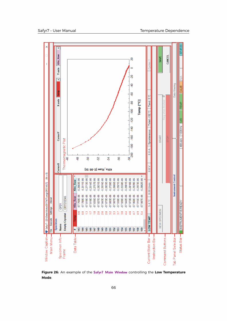
Safyr7 – User Manual Temperature Dependence
Figure 26: An example of the Safyr7 Main Window controlling the Low Temperature
Mode.
66
Safyr7 – User Manual Temperature Dependence
The thermomagnetic curves are saved into a fixed-column-width ASCII text file –
clw-file (FileName.clw). Each curve must be saved into a separate clw-file. When
applicable, a separate file (FileName_Im.clw ) is automatically created to store the
out-of-phase susceptibility thermomagnetic curves20.As the curve acquisition is a long lasting process, the measured
data are automatically appended into a temporary data file:
C:\Agico\Data\TemporaryData\SpecimenName.clw. This file may be use-
ful to recover the data in case that the data acquisition is forcefully
aborted (software crash, power blackout...etc.).
20Applies to the KLY5 models only.
67
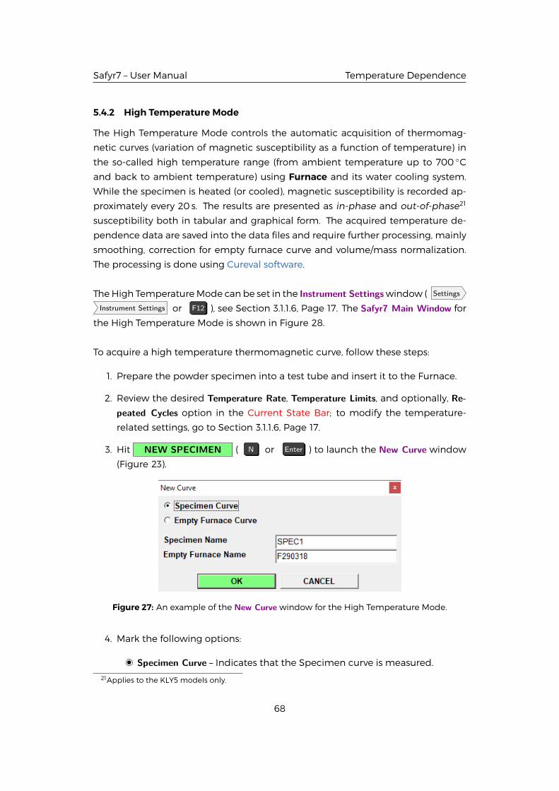
Safyr7 – User Manual Temperature Dependence
5.4.2 High Temperature Mode
The High Temperature Mode controls the automatic acquisition of thermomag-
netic curves (variation of magnetic susceptibility as a function of temperature) in
the so-called high temperature range (from ambient temperature up to 700 ◦C
and back to ambient temperature) using Furnace and its water cooling system.
While the specimen is heated (or cooled), magnetic susceptibility is recorded ap-
proximately every 20 s. The results are presented as in-phase and out-of-phase21
susceptibility both in tabular and graphical form. The acquired temperature de-
pendence data are saved into the data files and require further processing, mainly
smoothing, correction for empty furnace curve and volume/mass normalization.
The processing is done using Cureval software.
TheHigh TemperatureMode can be set in the Instrument Settings window ( Settings
Instrument Settings or F12 ), see Section 3.1.1.6, Page 17. The Safyr7 Main Window for
the High Temperature Mode is shown in Figure 28.
To acquire a high temperature thermomagnetic curve, follow these steps:
1. Prepare the powder specimen into a test tube and insert it to the Furnace.
2. Review the desired Temperature Rate, Temperature Limits, and optionally, Re-peated Cycles option in the Current State Bar; to modify the temperature-
related settings, go to Section 3.1.1.6, Page 17.
3. Hit NEW SPECIMEN ( N or Enter ) to launch the New Curve window
(Figure 23).
Figure 27: An example of the New Curve window for the High Temperature Mode.
4. Mark the following options:
Specimen Curve – Indicates that the Specimen curve is measured.
21Applies to the KLY5 models only.
68
Safyr7 – User Manual Temperature Dependence
Empty Furnace Curve – Indicates that the Empty Furnace curve is mea-
sured.
Fill the following text boxes:
• Specimen Name – Specimen namemust be up to 12 characters, no spaces,
comma or semicolons are allowed.
• Empty Furnace Name – Optionally, input the file name containing the re-
spective empty furnace thermomagnetic curve (it must be in the same
directory as the specimen data file). This information serves as a note
useful for further data processing. Please note that one empty furnace
thermomagnetic curve may be used for many specimen curves.
5. Hit OK ( Enter ) to confirm. The New Curve window is closed
and the specimen information is copied into the Specimen Info Frame of the
Safyr7 Main Window.
6. Hit START ( Enter ) to start the acquisition of thermomagnetic curve.
Hit STOP ( Space Bar ) to abort the curve acquisition in the case of
emergency.
7. The specimen starts to be heated (cooled) in a controlled way following the
preset Temperature Rate. As the temperature increases/decreases, magnetic
susceptibility is automatically measured approximately every 20 s. The actual
measuring procedure consists of the following actions:
(a) The instrument is zeroed.
(b) Specimen temperature is read and displayed in the Current State Bar.
(c) Cryostat automatically moves down into the pick up coil. pick up coil.
(d) Bulk susceptibility is measured.
(e) Cryostat automatically moves up from the pick up coil.
(f) Specimen temperature is read and displayed in the Current State Bar.
8. The average temperature (from the pre- and post measurement temperature
readings) andmeasured susceptibility values are appended to the Data Table
and the Thermomagnetic Plot is continuously re-drawn (Figure 28).
9. The steps 7 and8 are repeateduntil thedesiredmaximumtemperature (Tpeak)is reached, and then the controlled cooling starts until the desired minimum
temperature (Tend) is reached. The thermomagnetic curve is terminated and
a message box displaying termination time and measurement duration ap-
pears. Optionally, when selected, a ring tone sounds.
69
Safyr7 – User Manual Temperature Dependence
10. • Hit SAVE ( Enter or S ) to save themeasured thermomagn-
tic curve into a data file. As each curve must be saved into a separate file,
the Save Data dialog is automatically launched and the user must select
the file name (the file name derived from the current specimen name is
offered as a default option).
OR
• Hit CANCEL ( Esc ) to delete the results without saving.
Wait – Temperature is too high!When the curve acquisition is forcefully aborted, the temperature inside
the furnace may be very high! The warning starts flashing in the Instruc-
tion Bar. The furnace temperature spontaneously decreases towards the
ambient temperature and the warning stops when the temperature drops
below 100 ◦C.
The thermomagnetic curves are saved into a fixed-column-width ASCII text file –
cur-file (FileName.cur). Each curve must be saved into a separate cur-file. When
applicable, a separate file (FileName_Im.cur) is automatically created to store the
out-of-phase susceptibility thermomagnetic curves22.As the curve acquisition is a long lasting process, the measured
data are automatically appended into a temporary data file:
C:\Agico\Data\TemporaryData\SpecimenName.cur. This file may be use-
ful to recover the data in case that the data acquisition is forcefully
aborted (software crash, power blackout...etc.).
22Applies to the KLY5 models only.
70
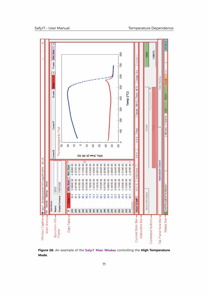
Safyr7 – User Manual Temperature Dependence
Figure 28: An example of the Safyr7 Main Window controlling the High Temperature
Mode.
71


Safyr7 – User Manual Appendix
6 Appendix
6.1 Specimen Positions
Figure29: Definition of the SpecimenCoordinate System for cylindrical and cubic spec-
imens.
Figure 30: The orientation of the calibration standard in manual specimen holders.
73
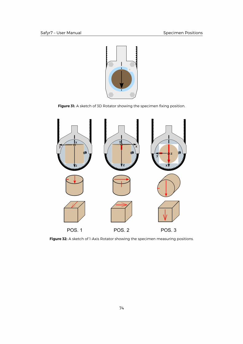
Safyr7 – User Manual Specimen Positions
Figure 31: A sketch of 3D Rotator showing the specimen fixing position.
Figure 32: A sketch of 1-Axis Rotator showing the specimen measuring positions.
74
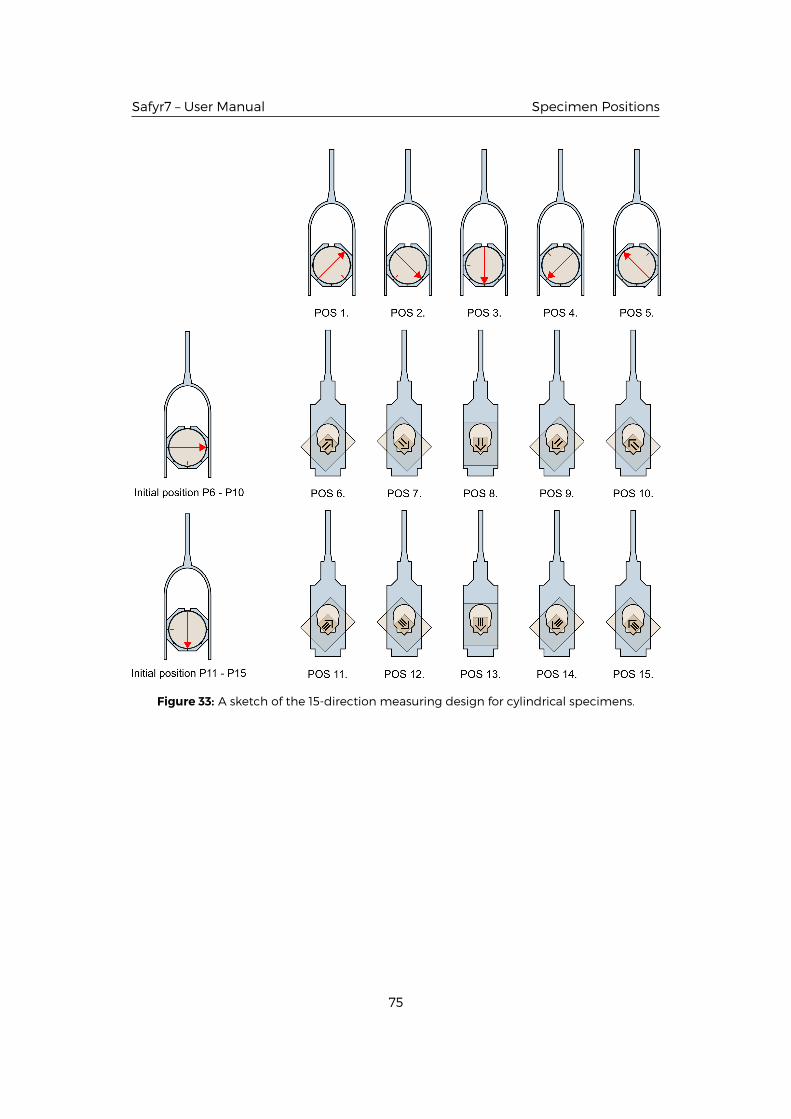
Safyr7 – User Manual Specimen Positions
Figure 33: A sketch of the 15-direction measuring design for cylindrical specimens.
75
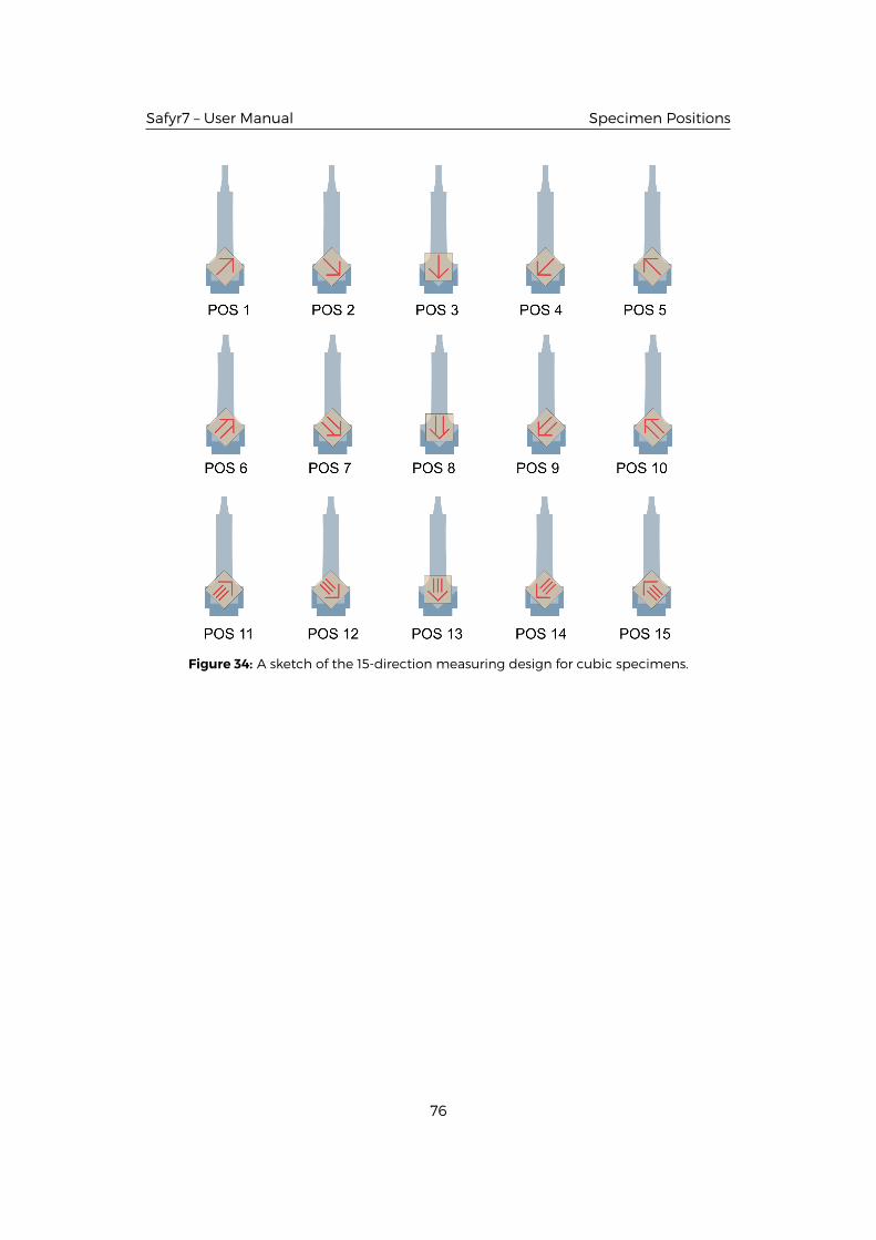
Safyr7 – User Manual Specimen Positions
Figure 34: A sketch of the 15-direction measuring design for cubic specimens.
76
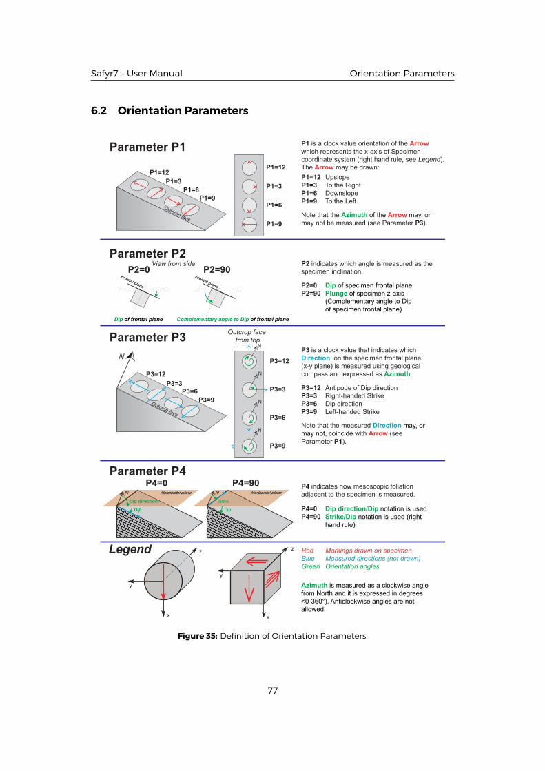
Safyr7 – User Manual Orientation Parameters
6.2 Orientation Parameters
P1=12
P3=12
P1=12
P1=3
P3=3
P1=3
P1=6
P3=6
P1=6
P1=9
P3=9
P2=0
P1=9
P2=90
Dip of frontal plane
P3=12
P3=3P3=6
P3=9
N
N
N
N
P4=0 P4=90
Dip Dip
N
Legend
x
y
x
y
zz
N N
Strike
Parameter P1
Parameter P2
Parameter P3
Parameter P4
P1 is a clock value orientation of the Arrow
which represents the x-axis of Specimen
coordinate system (right hand rule, see Legend).
The Arrow may be drawn:
P1=12 Upslope
P1=3 To the Right
P1=6 Downslope
P1=9 To the Left
Note that the Azimuth of the Arrow may, or
may not be measured (see Parameter P3).
Outcrop face
from top
Outcrop face
Outcrop face
View from side
Complementary angle to Dip of frontal plane
Frontal plane
Frontal plane
P2 indicates which angle is measured as the
specimen inclination.
P2=0 Dip of specimen frontal plane
P2=90 Plunge of specimen z-axis
(Complementary angle to Dip
of specimen frontal plane)
P3 is a clock value that indicates which
Direction on the specimen frontal plane
(x-y plane) is measured using geological
compass and expressed as Azimuth.
P3=12 Antipode of Dip direction
P3=3 Right-handed Strike
P3=6 Dip direction
P3=9 Left-handed Strike
Note that the measured Direction may, or
may not, coincide with Arrow (see
Parameter P1).
P4 indicates how mesoscopic foliation
adjacent to the specimen is measured.
P4=0 Dip direction/Dip notation is used
P4=90 Strike/Dip notation is used (right
hand rule)
Red Markings drawn on specimen
Blue Measured directions (not drawn)
Green Orientation angles
Azimuth is measured as a clockwise angle
from North and it is expressed in degrees
<0-360°). Anticlockwise angles are not
allowed!
Figure 35: Definition of Orientation Parameters.
77
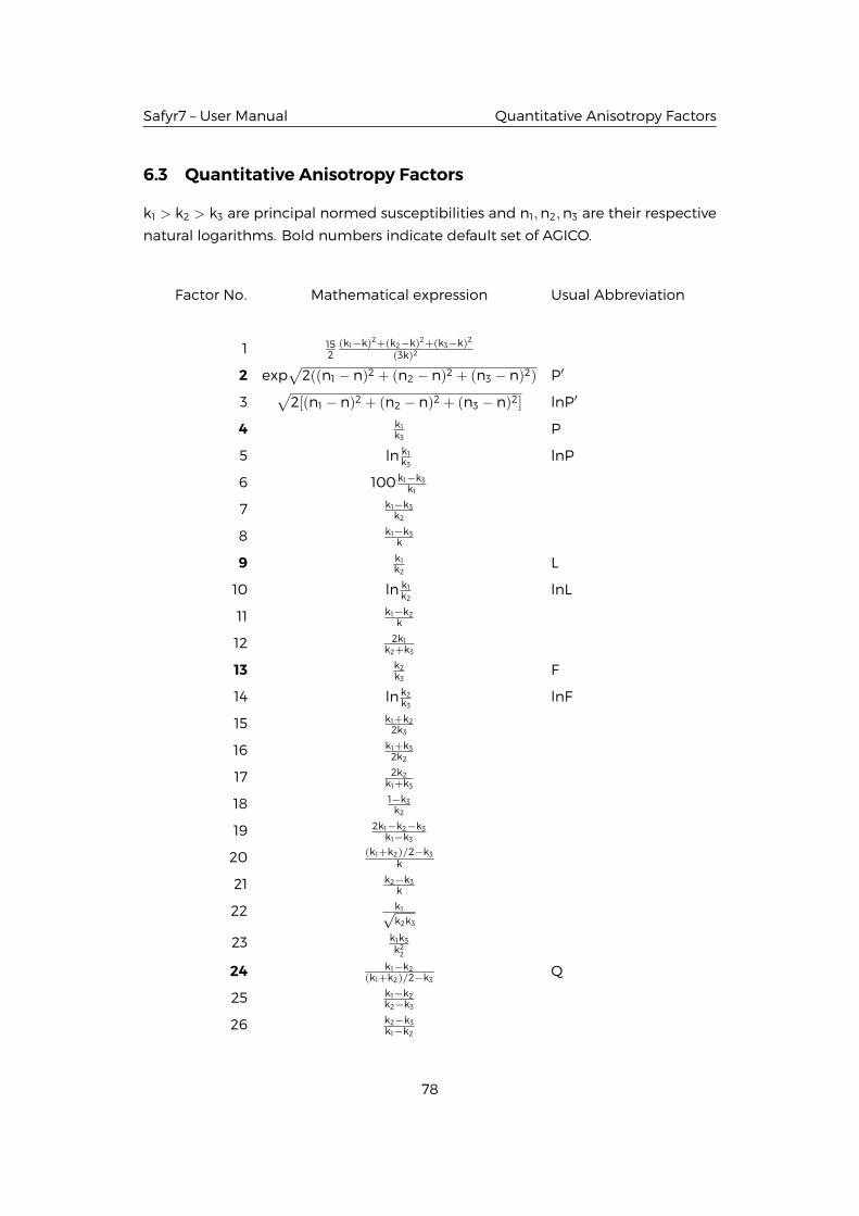
Safyr7 – User Manual Quantitative Anisotropy Factors
6.3 Quantitative Anisotropy Factors
k1 > k2 > k3 are principal normed susceptibilities and n1,n2,n3 are their respective
natural logarithms. Bold numbers indicate default set of AGICO.
Factor No. Mathematical expression Usual Abbreviation
1 152
(k1−k)2+(k2−k)2+(k3−k)2
(3k)2
2 exp√2((n1 − n)2 + (n2 − n)2 + (n3 − n)2) P′
3√2[(n1 − n)2 + (n2 − n)2 + (n3 − n)2] lnP′
4 k1k3
P
5 ln k1k3
lnP
6 100k1−k3k1
7 k1−k3k2
8 k1−k3k
9 k1k2
L
10 ln k1k2
lnL
11 k1−k2k
12 2k1k2+k3
13 k2k3
F
14 lnk2k3
lnF
15 k1+k22k3
16 k1+k32k2
17 2k2k1+k3
18 1−k3k2
19 2k1−k2−k3k1−k3
20 (k1+k2)/2−k3k
21 k2−k3k
22 k1√k2k3
23 k1k3k22
24 k1−k2(k1+k2)/2−k3
Q
25 k1−k2k2−k3
26 k2−k3k1−k2
78

Safyr7 – User Manual Quantitative Anisotropy Factors
27 arcsin√
k2−k3k1−k3
28 k22
k1k3E
29 k2k1−k2
k1(k2−k3)
30 k2/k3−1k1/k2−1
31 2n2−n1−n3n1−n3
T
32 2k2−k1−k3k1−k3
U
33 k1+k2−2k3k1−k2
34√
((k1−k)2+(k2−k)2+(k3−k)2)/3k R
35 (k1k2k3)13
36 k3(k1−k2)k1(k2−k3)
37 k3(k1−k2)
k22−k1k3
38 (k1−k2)(2k1−k2−k3)(k2−k3)(k1+k2−2k3)
79


![Chapter 2 Based on Anisotropy of Magnetic Susceptibility › pdfs › 59029.pdf · rocks and kinematics of deformation in metamorphic rocks [7]. Commonly, the flattening of the AMS](https://img.pdfslide.us/doc/110x75/5f1f2a83108ae2758569de4b/chapter-2-based-on-anisotropy-of-magnetic-susceptibility-a-pdfs-a-59029pdf.jpg)