Embed Size (px)
Citation preview
MECHANOBIOLOGICAL COMPUTATIONAL
MODEL FOR THE DEVELOPMENT AND
FORMATION OF SYNOVIAL JOINTS
Kalenia María Márquez Flórez
Universidad Nacional de Colombia, Faculty of Engineering,
Department of Mechanics and Mechatronic Engineering
Bogotá D.C., Colombia
Universitat de València, Faculty of Medicine and Odontology
Department of Pathology
Valencia, Spain
June 2019

MECHANOBIOLOGICAL COMPUTATIONAL
MODEL FOR THE DEVELOPMENT AND
FORMATION OF SYNOVIAL JOINTS
This Dissertation is submitted in partial fulfillment of the
requirements for the Degree of Philosophiae Doctor (PhD):
Kalenia Márquez-Flórez
Advisors:
María Sancho-Tello Valls
Carmen Carda Batalla
Diego Garzón Alvarado
Investigation Line:
Computational Mechanics and Tissular Engineering
Research Groups:
Grupo Modelado y Métodos Numéricos en Ingeniería-GNUM
Universidad Nacional de Colombia, Faculty of Engineering
Department of Mechanics and Mechatronic Engineering
Bogotá D.C., Colombia
Universitat de València, Faculty of Medicine and Odontology
Department of Pathology
Valencia, Spain
June 2019
Kalenia Márquez-Flórez
Mechanobiological computational model for the development and
formation of synovial joints, © 2019
Advised by: María Sancho-Tello Valls, Carmen Carda Batalla, Diego
Garzón Alvarado
Cover illustration: Kalenia Márquez Flórez
Universidad Nacional de Colombia
Universitat de València

Maria Sancho-Tello Valls, Doctora en Medicina i Cirurgia, Professora
Titular del Departament de Patologia de la Universitat de València;
Carmen Carda Batalla, Doctora en Medicina i Cirurgia, Doctora en
Odontologia, Catedràtica del Departament de Patologia de la Universitat de València;
i
Diego Alexander Garzón Alavarado, Doctor en Mecànica Computacional,
Full Professor del Departament d’Enginyeria Mecànica i Mecatrònica de la
Universidad Nacional de Colombia,
FAN CONSTAR QUÈ:
dins del Programa de Doctorat en Medicina, Kalenia María Márquez Flórez
ha realitzat, sota la seua direcció, del treball titulat Mechanobiological computational
model for the development and formation of synovial joints, que es presenta en aquesta
memòria per optar al grau de Doctor per la Universitat de València en cotutela amb la
Universidad Nacional de Colombia.
I per tal què així conste a efectes oportuns, i donant el vistiplau per a la
presentació d’aquest treball davant el Tribunal de tesi que corresponga, signen el
present certificat a València, Març de 2019.
_____________________________________
María Sancho-Tello Valls Professora Titular - Universitat de València
_____________________________________
Carmen Carda Batalla Catedràtica - Universitat de València
_____________________________________
Diego Alexander Garzón Alvarado
Full professor - Universidad Nacional de Colombia


A mi familia.
“Pero ustedes saben señores muy bien cómo es esto.
No nos falló la intención, pero sí el presupuesto…”
Dos colores: Blanco y negro, Jorge Drexler

i | P a g e
AGRADECIMIENTOS
Por medio de esta nota quiero agradecer a todos los que, directa o
indirectamente, aportaron en el desarrollo de mi tesis. Principalmente,
quiero agradecer a mis directores, empezando por el Prof. Diego Garzón,
quien me ha acogido e introducido en este mundo de la investigación desde
que dejé mis estudios de pregrado, pasando por la maestría y ahora en
doctorado (seguro tiene mucha paciencia). Quisiera agradecer a mis
directoras, Dra. Carmen Carda y Dra. María Sancho-Tello, por acogerme
en su casa, su universidad, y permitirme la oportunidad de trabajar en un
tema totalmente nuevo y desafiante para mí. Sí, a ellos tres les agradezco
por su guía durante el curso de mi doctorado, como estudiante, como
persona y como una investigadora inexperta. También quiero agradecerles
por la posibilidad que me dieron de hacer mi doctorado en cotutela entre
la Universidad Nacional de Colombia y la Universitat de València.
A mis padres, Francisco Márquez e Iveth Flórez, a mi hermano, Blake
Márquez, y al resto de mi familia, que con su paciencia, apoyo y ánimos
me sostuvieron durante los buenos momentos y las dificultades. Gracias a
ellos he llegado a este importante momento de mi vida.
A mis amigos, a Saúl M. a Nataly G., y en especial a Yesid Suárez, gracias
por su apoyo constante en todo lo que se me ocurre. Al equipo de
Taekwondo de la U. Nacional de Colombia. por permitirme disfrutar de su
compañía y campeonatos. A mis compañeros de doctorado, especialmente
a Héctor C. y Juan V., sus consejos y apoyo moral y académico fue, y
seguirá siendo, invaluable para mí. A Yesid V., por ayudarme desde la
distancia y por sus charlas ñoñas interesantes que me subían el ánimo.
A los que me han adoptado durante mi estancia en Valencia; al grupo de
Taekwondo de la U. de Valencia; a Karina por acogerme en su hogar, a
Sergio por subirme el ánimo cada vez, por la ayuda en la corrección de
estilo departes del documento.
Por último, agradezco a la Universidad Nacional de Colombia, Alma Mater
que me ha cobijado estos años, y a la que le debo lo que soy ahora. A la
Universitat de València, por acogerme y mostrarme un mundo académico
diferente al que conocía.

iii | P a g e
TABLE OF CONTENTS
Agradecimientos ......................................................................................................... i
Table of contents....................................................................................................... iii
List of Tables ........................................................................................................... vii
List of Figures........................................................................................................... ix
Abbreviations .......................................................................................................... xiii
Abstract .................................................................................................................... xv
Resumen................................................................................................................. xvii
Resum...................................................................................................................... xxi
General Introduction and Aim .................................................................................. 1
Chapter 1. Conceptual Background .......................................................................... 7
1.1. PRENATAL DEVELOPMENT .............................................................................. 7 1.1.1. Limbs ..................................................................................................... 10
1.1.2. Muscles and tendons ............................................................................. 13
1.1.3. Bone development ................................................................................. 14
1.1.4. Relevant time-line ................................................................................. 15
1.2. JOINTS ........................................................................................................... 17 1.2.1. Synovial Joints ...................................................................................... 19
1.2.2. Synovial joints structure ....................................................................... 21
1.2.3. Articular Cartilage................................................................................ 22
1.2.4. Cartilage diseases ................................................................................. 24
1.2.5. Subchondral bone ................................................................................. 26
1.3. FINITE ELEMENT METHOD (FEM) ................................................................. 28
Chapter 2. Joint Onset ............................................................................................. 31
2.1. INTRODUCTION .............................................................................................. 31
2.2. MATERIALS AND METHODS ........................................................................... 34 2.2.1. Biological Aspects Considered for the Joint Development Model ........ 34
2.2.2. Tissue Differentiation............................................................................ 37
2.2.3. Mathematical model for joint formation ............................................... 38
2.2.4. Growing of the tissue (Domain Growth) ............................................... 43
iv | P a g e
2.2.5. Numerical solution of PDEs. ................................................................. 44
2.2.6. Geometry, initial and boundary conditions, and simulated cases ......... 45
2.3. RESULTS ........................................................................................................ 47 2.3.1. Case I: interphalangeal joint development ........................................... 47
2.3.2. Case II: longer initial bud ..................................................................... 49
2.3.3. Case III: high growth rate ..................................................................... 50
2.3.4. Case IV: wider rudiment ....................................................................... 50
2.3.5. Case V: implantation of beads bearing GDF-5 (lateral) ...................... 52
2.3.6. Case VI: implantation of beads bearing GDF-5 (tip) ........................... 52
2.4. DISCUSSION ................................................................................................... 54
Chapter 3. Joint Morphogenesis ............................................................................. 61
3.1. INTRODUCTION .............................................................................................. 61
3.2. MATERIALS AND METHODS ............................................................................ 65 3.2.1. Geometry and boundary conditions ...................................................... 66
3.2.2. Mechanical Aspects ............................................................................... 67
3.2.3. Molecular Aspects ................................................................................. 68
3.2.4. Tissue Growth ....................................................................................... 70
3.2.5. Bone Ossification .................................................................................. 72
3.2.6. Translation to reference ........................................................................ 72
3.2.7. General algorithm ................................................................................. 73
3.2.8. Modelled cases ...................................................................................... 75
3.3. RESULTS ........................................................................................................ 76
3.4. DISCUSSION ................................................................................................... 83
Chapter 4. Patella Onset .......................................................................................... 91
4.1. INTRODUCTION .............................................................................................. 91
4.2. THEORY I: BIOCHEMICAL THEORY ................................................................. 93 4.2.1. Tendon & eminence development .......................................................... 95
4.2.2. Computational and mathematical model............................................... 96
4.2.3. Results and discussion ......................................................................... 104
4.3. THEORY II: MECHANICAL THEORY .............................................................. 108 4.3.1. Mathematical Model ........................................................................... 109
4.3.2. Geometry and boundary conditions .................................................... 111
4.3.3. Material properties and tissue differentiation ..................................... 112
4.3.4. Results and discussion ......................................................................... 112
4.4. THEORY III: TOPOLOGICAL OPTIMIZATION (TO) ......................................... 115 4.4.1. Geometry and boundary conditions .................................................... 118
4.4.2. Material properties ............................................................................. 119
4.4.3. Results and discussion ......................................................................... 119
4.5. NUMERICAL SOLUTION FOR THE THREE THEORIES ....................................... 120

v | P a g e
4.6. GENERAL DISCUSSION ................................................................................. 120
Chapter 5. Cartilage regeneration ........................................................................ 127
5.1. INTRODUCTION ............................................................................................ 127
5.2. MATERIALS AND METHODS .......................................................................... 131 5.2.1. Geometry and mesh............................................................................. 131
5.2.2. Boundary conditions ........................................................................... 133
5.2.3. Material Models .................................................................................. 134
5.2.4. General algorithm ............................................................................... 144
5.3. RESULTS ...................................................................................................... 147
5.4. DISCUSSION ................................................................................................. 152
Chapter 6. General conclusions and recommendations ....................................... 157
6.1. GENERAL CONCLUSIONS .............................................................................. 157
6.2. RECOMMENDATIONS ................................................................................... 160
Summary ................................................................................................................ 163
Summary in valencian ........................................................................................... 187
References .............................................................................................................. 213
Appendixes ............................................................................................................. 233
APPENDIX A – VALUE OF THE PARAMETERS USED ON CHAPTER 2 (JOINT ONSET)
........................................................................................................................... 233
APPENDIX B – VALUE OF THE PARAMETERS USED ON CHAPTER 4 (PATELLA
ONSET) ............................................................................................................... 235
APPENDIX C – VALUE OF THE PARAMETERS USED ON CHAPTER 5 (CARTILAGE
REGENERATION) ................................................................................................. 237
APPENDIX D – PUBLISHED AND SUBMITTED WORKS ........................................... 239
APPENDIX E – JOURNALS’ PERMISSIONS ............................................................. 241


vii | P a g e
LIST OF TABLES
Table 2-1 Tissue transformation criteria. ............................................................................... 38
Table 3-1 Conditions for the normal and pathological settings. ............................................. 75
Table 4-1 Relation between molecules and tissue or cell type for the model developed for
theory I. ................................................................................................................................. 101
Table 4-2 Molecule and threshold (Th) levels involved in the tissue differentiation. ............ 102
Table 4-3 Tissue properties ................................................................................................... 112

ix | P a g e
LIST OF FIGURES
Fig. 1-1 Timeline of the human prenatal development. ............................................................. 7
Fig. 1-2 Schematic representation of embryo development from the two-cell state to
blastocyst. ................................................................................................................................. 9
Fig. 1-3 Schematic representation of the human blastocyst components at second week. ...... 10
Fig. 1-4 Schematic representation of the development of the limb. ......................................... 11
Fig. 1-5 Scheme of human hand development. ........................................................................ 12
Fig. 1-6 Schematic representation of the muscle development in a 7-week embryo................ 13
Fig. 1-7 Schematic representation of the endochondral ossification of long bones. ............... 15
Fig. 1-8 Relevant timeline for human limb development. ........................................................ 16
Fig. 1-9 Schematic representation of the parts of a synovial joint. ......................................... 21
Fig. 1-10 3D schematic representation of the hyaline (articular) cartilage. ........................... 23
Fig. 1-11 Schematic representation of a finite element mesh. ................................................. 30
Fig. 2-1 Scheme of the stages of the synovial joints during the interphalangeal joint
development. ........................................................................................................................... 33
Fig. 2-2 Molecule concentration for each element. ................................................................. 38
Fig. 2-3 Relationship between enzyme (u) and substrate (v) for the Schnakenberg model
(enzyme-substrate). ................................................................................................................. 39
Fig. 2-4 Schematic of the boundary conditions employed for the joint onset model. .............. 46
Fig. 2-5 Results obtained by the simulation for case I. ........................................................... 48
Fig. 2-6 Results obtained by simulation for cases II, III and IV. ............................................. 51
Fig. 2-7 Results obtained by simulation for cases V and VI. ................................................... 53
Fig. 2-8 Comparison of the molecular distribution between the obtained results for case I
with those reported in former experimental studies. ............................................................... 56
Fig. 3-1 Schematic representation of the boundary conditions implemented on the model. ... 66
Fig. 3-2 Geometry of the bone anlagen and the synovial capsule. .......................................... 68
Fig. 3-3 Schematic definition of the concentration areas. ....................................................... 70
Fig. 3-4 Translation process from a rotated state to the reference state at (0º). ..................... 73
Fig. 3-5 Algorithm designed for joint morphogenesis. ............................................................ 74
Fig. 3-6 Geometry of the pathological kilter model. ............................................................... 76
Fig. 3-7 Obtained joint shape at different time-steps for normal conditions. .......................... 77
Fig. 3-8 Stress distribution at different time-steps. ................................................................. 78

x | P a g e
Fig. 3-9 Obtained joint shape at different unit time for the pathological condition when the
effect of the molecules is not included. ................................................................................... 79
Fig. 3-10 Obtained hydrostatic and octahedral stresses at different unit time for the w/o
molecular effect pathological setting. ..................................................................................... 79
Fig. 3-11 Obtained joint shape at different unit time for the simulated pathological
environments. Palmar side to the left and dorsal to the right. ................................................ 81
Fig. 3-12 Obtained hydrostatic and octahedral stresses at different unit time for the
pathological models. ............................................................................................................... 82
Fig. 3-13 Molecular distribution at different time-steps. ........................................................ 84
Fig. 3-14 Secondary ossification center (SOC) in a developing bone. ................................... 86
Fig. 3-15 Comparison of the obtained geometries for the kilter, the 0º palsy, the 90º palsy and
the normal conditions ............................................................................................................. 87
Fig. 4-1 Sagittal sections of the patella from hind limbs of wild-type mouse embryos stained
with Alcian Blue and Fast Red to highlight cartilage cells (I. A-C) and Sox9 and Scx
expression (II). ........................................................................................................................ 94
Fig. 4-2 Schematic representation of the tendon and eminence development. ....................... 95
Fig. 4-3 Schematic representation of the patella development process based on the theory
proposed by Eyal et al. [117]. ................................................................................................ 97
Fig. 4-4 General algorithm that developed to model the events occurring according to the
Theory I. ................................................................................................................................. 99
Fig. 4-5 Knee joint geometry employed for patella development study. ............................... 103
Fig. 4-6 Obtained distribution of the molecules (TGF-β, BMP, FGF, GDF-5) and Scx-cells
during patella development. ................................................................................................. 106
Fig. 4-7 Obtained tissue differentiation through the time of patella development. ............... 107
Fig. 4-8 Patella development: tissue differentiation for the biochemical model at different
angles (60°, 45° and 30°). .................................................................................................... 107
Fig. 4-9 Diagram of the mechanoregulatory model proposed by Carter et al., (1998) [7]. . 109
Fig. 4-10 Schematic representation of the geometry and boundary conditions. ................... 111
Fig. 4-11 Results obtained by the simulation for the different angles: stress, tensile strain and
patella shape......................................................................................................................... 114
Fig. 4-12 Results obtained by the simulation for the average hydrostatic stress and patella
shape. ................................................................................................................................... 115
Fig. 4-13 Results obtained by the simulation through the TO algorithm. ............................. 120
Fig. 5-1 Schematic representation of the 2D finite element geometry of the articular surface
and subchondral bone, with the scaffold implanted.............................................................. 132
Fig. 5-2 Boundary conditions applied to the finite element model. ...................................... 133

xi | P a g e
Fig. 5-3 Graphic of the angle of the fibers at each zone. ...................................................... 135
Fig. 5-4 Flow chart of the employed algorithm for cartilage or bone regeneration. ............ 146
Fig. 5-5 Simulation of tissue differentiation after scaffold implantation throughout the
simulation. ............................................................................................................................. 149
Fig. 5-6 Simulation of collagen fiber orientation after implantation. ................................... 150
Fig. 5-7 Simulation of bones’ Young’s modulus after scaffold implantation. ....................... 151
Fig. 5-8 Comparison of our results with the histological findings of a previous experimental
study. ..................................................................................................................................... 156
Declaration: Figures without reference were done by the authors.

xiii | P a g e
ABBREVIATIONS
Abbreviation Definition
AER Apical Ectodermal Ridge
BMP Bone Morphogenetic Protein
CA Cellular Automaton
DDH Developmental Dysplasia of the Hip
DZ Deep Zone
ECM Extracellular Matrix
FEA Finite Element Analysis
FEM Finite Element Method
FGF Fibroblast Growth Factor
FV Fluid Velocity
GDF Growth Differentiation Factor
Ihh Indian hedgehog signaling molecule
MS Mechanical stimulation
OA Osteoarthritis
OI Osteogenic Index
PDE Partial Differential Equation
POC Primary Ossification Center
PTHrP Parathyroid Hormone-related Protein
PVF Potential Vascularity Factor
RA Rheumatoid Arthritis
RZ Radial Zone
SIMP Solid Isotropic Material with Penalization
SOC Secondary Ossification Center
SZ Superficial Zone
TGF-β Transforming Growth Factor-β
TO Topological Optimization
σ Stress


xv | P a g e
ABSTRACT
The onset and development of the synovial joints is due to
different genetic, biochemical, and mechanical factors. It starts at the
limb buds, which have an uninterrupted mass of mesenchymal cells
within its core, also known as skeletal blastema. Most of these blastemal
cells differentiate into chondrocytes; however, some of these cells
remain undifferentiated at the site of the future joint (interzone). The
separation of the rudiments occurs with cavitation process within the
interzone. After the joint cleavage (cavitation), joint morphogenesis
occurs, and the bones take their final shape. Once the embryonic period
has finished, the synovial joint and its internal structures has developed
completely. Though, once the synovial joints are formed, they might
suffer several pathologies, such as the osteoarthritis (OA). There are
several treatments that have been proposed to regenerate the articular
cartilage, among which scaffolds without cellular sources have shown
great results.
Understand the processes that the joint tissue goes through are
important to develop new direct and effective treatments for joint
related pathologies. Computational models seem a good alternative tool
to complement the study of the joint processes. Therefore, it was of our
interest to study, through computational models, the biochemical
interaction for the interzone onset, the cavitation and morphogenesis
processes during the joint development. We analyzed these phenomena
within the development of an interphalangeal joint and the patella onset.
Moreover, we were also interested on analyzing, through a
computational model, the processes happening when a defect in the
articular cartilage is treated with the implantation of a polymeric
scaffold.
All the computational models developed in this study applied
theories about tissue behavior under mechanical and biochemical
xvi | P a g e
stimuli. The obtained results were compared to experimental works
found in the literature, all of them showed promising outcomes. Hence,
we consider that the procedures and considerations taken for each
proposed computational model are not far from what is really
happening on the analyzed biological phenomena. Moreover, we were
able to evaluate mechanical and biochemical conditions the biological
phenomena, that would be hard to test through experimental
approaches. We hope that these models become useful to medical and
biological researches, helping in the design of prevention and therapy
strategies for joint related diseases.
This thesis is structured in eight parts including an introduction
which tries to aware the importance of the study and the objectives of
the thesis. Afterwards, on the second part, we expose some general
concepts related to the topics and methods employed to develop the
research. Then, the third part describes a computational model proposed
to explain joint development from the interzone onset to the cavitation
process. The fourth part is focus on the joint morphogenesis as part of
the joint development process. Subsequently, the fifth section is
dedicated to explaining the sesamoid bones development through a
comparison of three theories of the patella onset, evaluated via
computational models. The seventh part of this work is a computational
model proposed to understand the processes that surround the cartilage
regeneration when a polymeric scaffold is implanted in the articular
cartilage. In the last part, we concluded the achievements and discussed
the main conclusions of the thesis, as well as the recommended future
work and perspectives. As an additional chapter, we added a general
overview of the thesis in English and in Valencian.

xvii | P a g e
RESUMEN
El desarrollo de las articulaciones sinoviales se debe a diferentes
factores genéticos, bioquímicos y mecánicos. Comienza en el brote de
las extremidades, que tienen una masa ininterrumpida de células
mesenquimales dentro de su núcleo, el blastema esquelético. La
mayoría de estas células blastemales se diferencian en condrocitos; sin
embargo, algunas de estas células permanecen, sin diferenciar, en el
sitio de la futura articulación (interzona). La separación de los
rudimentos ocurre con el proceso de cavitación dentro de la interzona.
Después de la cavitación, se produce la morfogénesis articular y el
hueso toma su forma final. Una vez finalizado el período embrionario,
la articulación sinovial y sus estructuras internas se han desarrollado
completamente. Aunque una vez que se forman las articulaciones
sinoviales, pueden sufrir, a lo largo de la vida, distintas patologías,
como la osteoartritis (OA). Hay varios tratamientos que se han
propuesto para regenerar el cartílago articular, entre los cuales, los
andamiajes (scaffolds) sin fuentes celulares han mostrado grandes
resultados.
Comprender los procesos por los que pasa el tejido articular es
importante para desarrollar nuevos tratamientos directos y efectivos
para las patologías relacionadas con las articulaciones. Los modelos
computacionales parecen ser una buena herramienta para
complementar el estudio de los procesos articulares. Por lo tanto, fue de
nuestro interés estudiar, a través de modelos computacionales, la
interacción bioquímica de la aparición de la interzona, la cavitación y
la morfogénesis durante el desarrollo de articulaciones. Analizamos
estos fenómenos en el desarrollo de una articulación interfalángica y el
desarrollo de la rótula. Además, también estábamos interesados en
analizar, mediante un modelo computacional, los procesos que ocurren
xviii | P a g e
cuando un defecto en el cartílago articular se trata con la implantación
de un andamiaje polimérico.
Todos los modelos computacionales desarrollados en este
estudio aplicaron teorías sobre el comportamiento de los tejidos bajo
estímulos mecánicos y bioquímicos. Los resultados obtenidos, fueron
comparados con los trabajos experimentales encontrados en la
literatura, todos los modelos mostraron resultados prometedores. Por lo
tanto, consideramos que los procedimientos y las suposiciones tomadas
para cada modelo computacional propuesto no están lejos de lo que
realmente está sucediendo en los fenómenos biológicos analizados.
Además, pudimos evaluar las condiciones mecánicas y bioquímicas de
los fenómenos biológicos analizados, difíciles de probar a través de
enfoques experimentales. Esperamos que estos modelos sean útiles para
las investigaciones médicas y biológicas, ayudando en el diseño de
estrategias de prevención y terapia para enfermedades relacionadas con
las articulaciones.
Esta tesis está estructurada en ocho partes, incluida una
introducción que trata de exponer la importancia del estudio y los
objetivos de la tesis. Posteriormente, en la segunda parte exponemos
algunos conceptos generales relacionados con los temas y métodos
empleados para desarrollar la investigación. Luego, la tercera parte
describe un modelo computacional propuesto para explicar el desarrollo
de articulaciones desde el inicio de la interzona hasta el proceso de
cavitación. La cuarta parte se centra en la morfogénesis de las
articulaciones como parte del proceso de desarrollo de las mismas.
Posteriormente, la quinta sección está dedicada a explicar el desarrollo
de los huesos sesamoideos a través de una comparación de tres teorías
del desarrollo de la rótula, evaluadas mediante modelos
computacionales. La séptima parte de este trabajo es un modelo
computacional propuesto para comprender los procesos que rodean la
regeneración del cartílago cuando se implanta un andamiaje polimérico
en el cartílago articular. En la última parte, se concluyen los logros y se
analizan las principales conclusiones de la tesis, así como el trabajo

xix | P a g e
futuro recomendado y las perspectivas. Como capítulo adicional,
agregamos una descripción general de la tesis en inglés y en valenciano.

xxi | P a g e
RESUM
El desenvolupament de les articulacions sinovials es deu a
diferents factors genètics, bioquímics i mecànics. Comença en el brot
de les extremitats, que tenen una massa ininterrompuda de cèl·lules
mesenquimals dins del seu nucli, el blastema esquelètic. La majoria
d'aquestes cèl·lules blastemales es diferencien en condròcits; però,
algunes d'aquestes cèl·lules, sense deferenciar, romanen en el lloc de la
futura articulació (interzona). La separació dels rudiments passa amb el
procés de cavitació dins de la interzona. Després de la cavitació, es
produeix la morfogènesi articular i l'os pren la seva forma final. Un cop
finalitzat el període embrionari, l'articulació sinovial i les seves
estructures internes s'han desenvolupat completament. Encara que, una
vegada que es formen les articulacions sinovials, poden patir diverses
patologies, com l'osteoartritis (OA). Hi ha diversos tractaments que
s'han proposat per regenerar el cartílag articular, entre els quals, les
bastides sense fonts cèl·lules han mostrat grans resultats.
Comprendre els processos pels quals passa el teixit articular és
important per desenvolupar nous tractaments directes i efectius per a les
patologies relacionades amb les articulacions. Els models
computacionals semblen ser una bona eina per complementar l'estudi
dels processos articulars. Per tant, va ser del nostre interès estudiar, a
través de models computacionals, la interacció bioquímica de l'aparició
de la interzona, la cavitació i la morfogènesi durant el desenvolupament
d'articulacions. Analitzem aquests fenòmens en el desenvolupament
d'una articulació interfalangica i el desenvolupament de la ròtula. A
més, també estàvem interessats en analitzar, mitjançant un model
computacional, els processos que ocorren quan un defecte en el cartílag
articular es tracta amb la implantació d'una bastida polimèric.
Tots els models computacionals desenvolupats en aquest estudi
van aplicar teories sobre el comportament dels teixits sota estímuls
xxii | P a g e
mecànics i bioquímics. Els resultats obtinguts, en comparació amb els
treballs experimentals trobats en la literatura, tots ells van mostrar
resultats prometedors. Per tant, considerem que els procediments i les
consideracions preses per a cada model computacional proposat no
estan lluny del que realment està succeint en els fenòmens biològics
analitzats. A més, vam poder avaluar les condicions mecàniques i
bioquímiques dels fenòmens biològics analitzats, que serien difícils de
provar a través d'enfocaments experimentals. Esperem que aquests
models siguin útils per a les investigacions mèdiques i biològiques,
ajudant en el disseny d'estratègies de prevenció i teràpia per a malalties
relacionades amb les articulacions.
Aquesta tesi està estructurat en vuit parts, inclosa una
introducció que tracta de conèixer la importància de l'estudi i els
objectius de la tesi. Posteriorment, a la segona part exposem alguns
conceptes generals relacionats amb els temes i mètodes emprats per a
desenvolupar la investigació. Després, la tercera part descriu un model
computacional proposat per explicar el desenvolupament
d'articulacions des de l'inici de la interzona fins al procés de cavitació.
La quarta part se centra en la morfogènesi de les articulacions com a
part del procés de desenvolupament de les articulacions. Posteriorment,
la cinquena secció està dedicada a explicar el desenvolupament dels
ossos sesamoideos a través d'una comparació de tres teories del
desenvolupament de la ròtula, avaluades mitjançant models
computacionals. La setena part d'aquest treball és un model
computacional proposat per comprendre els processos que envolten la
regeneració del cartílag quan s'implanta una bastida polimèric en el
cartílag articular. En l'última part, es conclouen els èxits i s'analitzen les
principals conclusions de la tesi, així com el treball futures recomanades
i les perspectives. Com capítol addicional, afegim una descripció
general de la tesi en anglès i en valencià.
1 | P a g e
GENERAL INTRODUCTION AND
AIM
Imagine how different human beings would be without the
flexibility of movements that their bodies owe to the joints. What would
have happened if their wrist would not have evolved to the complex
joint that it is now? Or what if the movement the hip had not been as
wide ranged as it is now? Would we have been able to walk erect?
Certainly, we would have been different, we would not be what we are
now. The liberty that our joints give us is priceless, they allow us to
move freely, to bend, to jump, to grab, to walk, to express our selves.
Now, wonder what would happen if you lose mobility of one of
your joints. Surely you would adapt, however, one can bet that at the
beginning you would feel like your freedom is being cutback; from then
on, your life wouldn’t be the same. But what if you were born with a
malformation on one of your joints? You might be used to the
limitation; after all, you have been living with it since birth. However,
on both mentioned cases, when compared to other human beings, you
would feel behind on your capacities, and depending on the
malformation or joint pathology, you would have to bear with other
health issues such as the degradation of articular cartilage of the joint,
or pain in other parts of your body due to a bad posture or movement.
Consequently, any joint disease brings a substantial drop in the quality
General Introduction and Aim
2 | P a g e
of life. Therefore, it should be of high interest to study, with all available
tools, how to prevent and treat joint-related diseases.
In general, joints are described as the site where two or more
bones meet and can be classified according to their structure (how they
are connected) and their function (how the movement between its bones
is) -on Conceptual Background these classifications are described-.
Within these classifications, the synovial joints, which also are
classified as diarthrosis joints, offer the wider range of motion between
bones. It is because of its range of motion and its structure that synovial
joints are susceptible to articular diseases such as OA. Also, because of
the complexity of the processes involved in its development, synovial
joints are susceptible to developmental diseases and malformations,
such as developmental dysplasia of the hip.
Synovial joint development is a complex process that initiates
on the fetal stages of the prenatal development. Around five weeks of
development, limb buds are noticeable. Initially, these limb buds have
an uninterrupted core of mesenchymal cells, skeletal blastema, covered
by a layer of ectoderm (future skin). Afterwards, these blastemal cells
differentiate into chondrocytes, except on the site of the future joints.
This area is known as the interzone, where the cavitation process takes
place allowing the separation of the bone rudiments. Then, the two
opposing cartilaginous rudiments acquire their reciprocal interlocking
shapes through the process known as morphogenesis. If there are
abnormal conditions during fetal development, joints can develop
incomplete or abnormal, or even they might not develop at all.
General Introduction and Aim
3 | P a g e
By the end of the embryonic period, if there were not any
abnormal conditions, the synovial joint has developed completely as
well as its internal structures, articular cartilage, ligaments and synovial
capsule. Moreover, the primary and secondary ossification centers of
the bone appear which let the bone grow and ossify until adulthood.
Once the joint is developed, there might be some pathologies
that still might impair the normal function of the joint. Among them,
the OA, in which the articular cartilage that covers the bone
degenerates. There are many causes, from idiopathic to related to
trauma, that might end in this disease. Moreover, morphologic
abnormalities (developmental diseases) may cause joint incongruities,
which modify the load transmission through the cartilage, generating
overloaded points that trigger early degeneration of joints. Different
treatments have been proposed ranging from symptomatic, with
analgesics and anti-inflammatory medications, to more invasive ones
such as endochondral transplantation; being the last resort arthrodesis
treatments, or total replacement of the joint. Nevertheless, it is
preferable to preserve the original function of the joint through the
regeneration of the articular cartilage, especially in young patients.
Among the cartilage regeneration treatments are included the
osteochondral grafts, which can be considered as the most effective one
[1,2]. However, these grafts have some disadvantages: patients must go
through two surgeries, they create new defects, they are not appropriate
for large defects, they become unstable with time, and normally the new
tissue is fibrocartilage but not hyaline cartilage (as the articular
cartilage) [1]. Recently, in the last 2 decades, cartilage regeneration has
General Introduction and Aim
4 | P a g e
been based on the use of scaffolds, which allow rapid filling of joint
defects, providing a substrate where cells can anchor while maintaining
mechanical integrity [3]. With scaffolds/cell-free implants, hyaline
(articular) cartilage is generated in the upper part of the scaffold while
it displaces into the subchondral bone [4].
Thanks to the growing literature regarding material properties
and mechanics of the human body, the use of computational models in
the field of biomechanics is expanding rapidly. This has made
computational models a useful tool to understand the biomechanical-
biochemical interactions that tissues go through during the regeneration
and development processes. Computational models contribute to the
evaluation of difficult to reach aspects for experimental models [5]. In
this way, computational models provide a quantitative and qualitative
evaluation of mechanobiological interactions while being fed with
clinical or experimental parameters [6].
The biological computational models have been very useful to
simulate biological processes: bone regeneration [7], bone growth [8],
pattern formation [9–15], and embryonic development [16]. For
cartilage, several computational models have been developed [5,17–
19]. However, there are none, to our knowledge, related to cartilage
regeneration. Regarding joint development, only two computational
studies have been developed, the first one was done by Heegaard et al.,
[20], in which they explored how motion affected joint morphogenesis;
and a second one developed by Giorgi et al., [21], who analyzed the
effect of movement range with different initial shapes of the joint.
General Introduction and Aim
5 | P a g e
Computational models might be useful to understand critical
factors that must be considered for the design of strategies for the early
diagnosis and prevention of joint developmental diseases. Also, it
would help to recognize factors that might influence how a joint can be
repaired. Moreover, computational models might help identify which
processes are involved in joint regeneration, and therefore, they can
help with the development of effective and direct treatments for treating
degenerative joint diseases, all in behalf of improving life quality.
Therefore, the main aim of this work is to computationally
model the mechanical and biological aspects during the development of
synovial joints. This main objective is divided in three specific ones.
First, to formulate the mathematical description of the
mechanobiological phenomena for the development of synovial joints.
Second, to computationally evaluate the behavior of the models for the
interzone onset Third, to computationally evaluate the behavior for the
cavitation and morphogenesis of synovial joints.
This work is organized into five parts. The first part (Joint
Onset) describes a computational model for the first stages of the joint
onset. It is explained, computationally, the appearance of the interzone
and cavitation processes of an interphalangeal joint. On the second part
(Joint Morphogenesis), a computational model for the last step of joint
formation, the morphogenesis process of an interphalangeal joint from
the sagittal view, is exposed. The third part (Patella Onset) explores
three different theories that may explain the development of the patella
bone (a sesamoid bone) through computational models. In the fourth
part (Cartilage regeneration), a computational model of the regeneration
General Introduction and Aim
6 | P a g e
of the articular cartilage when employing a polymeric scaffold is
described. Finally, the fifth part (General conclusions) contains the
conclusions extracted from the current study. Each part of the
developed work (Chapter 2 to Chapter 5) are structured as follows: an
introduction on the chapter's subjects, a description of the employed
methods and the obtained results, and a discussion of the results.
Additionally, prior to the description of the work developed here
was added a chapter (Conceptual Background) in which we expose a
brief portrayal of the fetal development, synovial joint structures
articular cartilage and the finite element method (FEM).
Statement: In this thesis the Chapter 2 (Joint Onset) and
Chapter 4 (Patella Onset) are from already published works of my
authorship: Permissions were obtained from the journals to include the
pre-print articles in this thesis (Appendix E – Journals’ permissions).
The articles are the following:
Chapter 2 - Joint Onset:
K.M. Márquez-Flórez, J.R. Monaghan, S.J. Shefelbine, A.
Ramirez-Martínez, D.A. Garzón-Alvarado, A computational model for
the joint onset and development, J. Theor. Biol. 454 (2018) 345–356.
doi:10.1016/j.jtbi.2018.04.015.
Chapter 4 - Patella Onset:
K. Márquez-Flórez, S. Shefelbine, A. Ramírez-Martínez, D.
Garzón-Alvarado, Computational model for the patella onset, PLoS
One. 13 (2018) e0207770. doi:10.1371/journal.pone.0207770.
7 | P a g e
Chapter 1. CONCEPTUAL
BACKGROUND
1.1. PRENATAL DEVELOPMENT
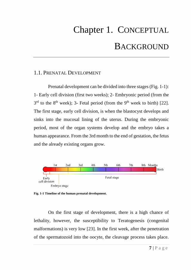
Prenatal development can be divided into three stages (Fig. 1-1):
1- Early cell division (first two weeks); 2- Embryonic period (from the
3rd to the 8th week); 3- Fetal period (from the 9th week to birth) [22].
The first stage, early cell division, is when the blastocyst develops and
sinks into the mucosal lining of the uterus. During the embryonic
period, most of the organ systems develop and the embryo takes a
human appearance. From the 3rd month to the end of gestation, the fetus
and the already existing organs grow.
Fig. 1-1 Timeline of the human prenatal development.
On the first stage of development, there is a high chance of
lethality, however, the susceptibility to Teratogenesis (congenital
malformations) is very low [23]. In the first week, after the penetration
of the spermatozoid into the oocyte, the cleavage process takes place.
Conceptual Background
8 | P a g e
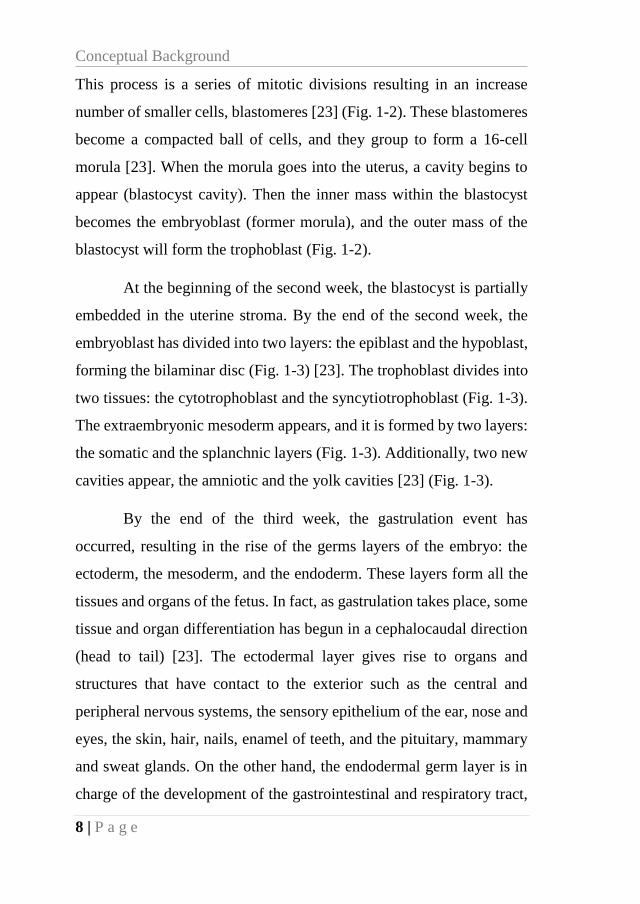
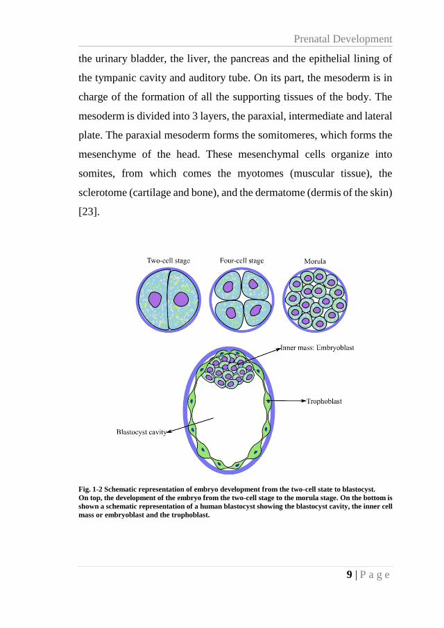
This process is a series of mitotic divisions resulting in an increase
number of smaller cells, blastomeres [23] (Fig. 1-2). These blastomeres
become a compacted ball of cells, and they group to form a 16-cell
morula [23]. When the morula goes into the uterus, a cavity begins to
appear (blastocyst cavity). Then the inner mass within the blastocyst
becomes the embryoblast (former morula), and the outer mass of the
blastocyst will form the trophoblast (Fig. 1-2).
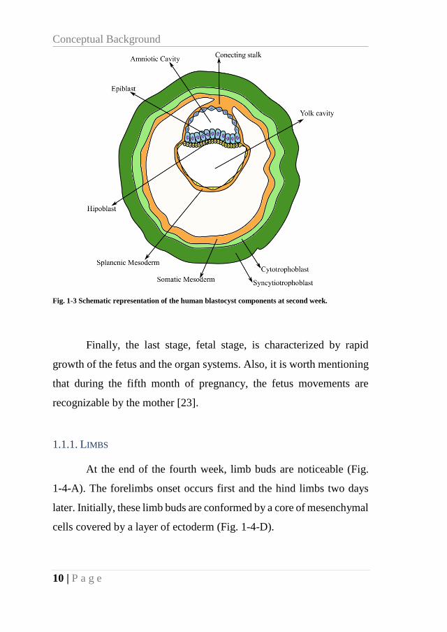
At the beginning of the second week, the blastocyst is partially
embedded in the uterine stroma. By the end of the second week, the
embryoblast has divided into two layers: the epiblast and the hypoblast,
forming the bilaminar disc (Fig. 1-3) [23]. The trophoblast divides into
two tissues: the cytotrophoblast and the syncytiotrophoblast (Fig. 1-3).
The extraembryonic mesoderm appears, and it is formed by two layers:
the somatic and the splanchnic layers (Fig. 1-3). Additionally, two new
cavities appear, the amniotic and the yolk cavities [23] (Fig. 1-3).
By the end of the third week, the gastrulation event has
occurred, resulting in the rise of the germs layers of the embryo: the
ectoderm, the mesoderm, and the endoderm. These layers form all the
tissues and organs of the fetus. In fact, as gastrulation takes place, some
tissue and organ differentiation has begun in a cephalocaudal direction
(head to tail) [23]. The ectodermal layer gives rise to organs and
structures that have contact to the exterior such as the central and
peripheral nervous systems, the sensory epithelium of the ear, nose and
eyes, the skin, hair, nails, enamel of teeth, and the pituitary, mammary
and sweat glands. On the other hand, the endodermal germ layer is in
charge of the development of the gastrointestinal and respiratory tract,
Prenatal Development
9 | P a g e
the urinary bladder, the liver, the pancreas and the epithelial lining of
the tympanic cavity and auditory tube. On its part, the mesoderm is in
charge of the formation of all the supporting tissues of the body. The
mesoderm is divided into 3 layers, the paraxial, intermediate and lateral
plate. The paraxial mesoderm forms the somitomeres, which forms the
mesenchyme of the head. These mesenchymal cells organize into
somites, from which comes the myotomes (muscular tissue), the
sclerotome (cartilage and bone), and the dermatome (dermis of the skin)
[23].
Fig. 1-2 Schematic representation of embryo development from the two-cell state to blastocyst.
On top, the development of the embryo from the two-cell stage to the morula stage. On the bottom is
shown a schematic representation of a human blastocyst showing the blastocyst cavity, the inner cell
mass or embryoblast and the trophoblast.
Conceptual Background
10 | P a g e
Fig. 1-3 Schematic representation of the human blastocyst components at second week.
Finally, the last stage, fetal stage, is characterized by rapid
growth of the fetus and the organ systems. Also, it is worth mentioning
that during the fifth month of pregnancy, the fetus movements are
recognizable by the mother [23].
1.1.1. LIMBS
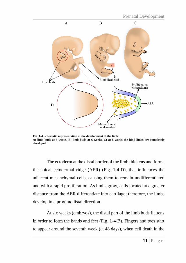
At the end of the fourth week, limb buds are noticeable (Fig.
1-4-A). The forelimbs onset occurs first and the hind limbs two days
later. Initially, these limb buds are conformed by a core of mesenchymal
cells covered by a layer of ectoderm (Fig. 1-4-D).
Prenatal Development
11 | P a g e
Fig. 1-4 Schematic representation of the development of the limb.
A: limb buds at 5 weeks. B: limb buds at 6 weeks. C: at 8 weeks the hind limbs are completely
developed.
The ectoderm at the distal border of the limb thickens and forms
the apical ectodermal ridge (AER) (Fig. 1-4-D), that influences the
adjacent mesenchymal cells, causing them to remain undifferentiated
and with a rapid proliferation. As limbs grow, cells located at a greater
distance from the AER differentiate into cartilage; therefore, the limbs
develop in a proximodistal direction.
At six weeks (embryos), the distal part of the limb buds flattens
in order to form the hands and feet (Fig. 1-4-B). Fingers and toes start
to appear around the seventh week (at 48 days), when cell death in the
Conceptual Background
12 | P a g e
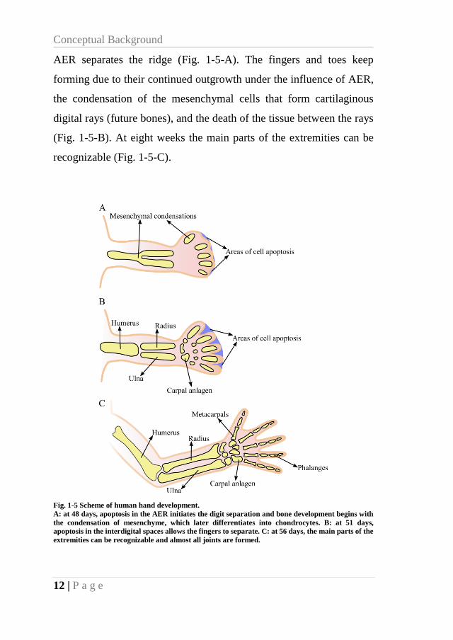
AER separates the ridge (Fig. 1-5-A). The fingers and toes keep
forming due to their continued outgrowth under the influence of AER,
the condensation of the mesenchymal cells that form cartilaginous
digital rays (future bones), and the death of the tissue between the rays
(Fig. 1-5-B). At eight weeks the main parts of the extremities can be
recognizable (Fig. 1-5-C).
Fig. 1-5 Scheme of human hand development.
A: at 48 days, apoptosis in the AER initiates the digit separation and bone development begins with
the condensation of mesenchyme, which later differentiates into chondrocytes. B: at 51 days,
apoptosis in the interdigital spaces allows the fingers to separate. C: at 56 days, the main parts of the
extremities can be recognizable and almost all joints are formed.

Prenatal Development
13 | P a g e
While the limb bud is shaping, the mesenchymal cells within the
buds begin to condense and differentiate into chondrocytes. At six
weeks, the shadowing of the first bone anlagen can be seen (Fig. 1-5-
A). Later, these bones anlages separate, forming the joints between
them (Fig. 1-5-B and Fig. 1-5-C).
1.1.2. MUSCLES AND TENDONS
Fig. 1-6 Schematic representation of the muscle development in a 7-week embryo.
A: seventh week, a condensation of mesenchymal cells from the myoblast is located near the base of
the limb buds. B: the myotome cells contribute to muscles, the dermatome cells form the dermis of
the back, and the sclerotome forms the tendons. C: cross section through half the embryo, the muscles
of the limbs start as a segmented structure that splits into the extensor and flexor muscles as the limb
grows.
During development, precursor cells from the myoblast fuse and
form long multinucleated muscle fibers. By the end of the third month,
myofibrils appear and organize in cross-striations [23]. On the limbs,
the first sheds of muscles can be observed after the seventh week as a

Conceptual Background
14 | P a g e
condensation of mesenchymal cells near the base of the limb buds (Fig.
1-6). The muscles start as a segmented structure that splits into the
extensor (dorsal) and flexor (ventral) muscles as the limb grow (Fig.
1-6); afterwards, additional splitting and fusions occur so that a single
muscle could be formed with several original segments. On the other
hand, tendons are formed by sclerotome cells. These cells are lying
adjacent to the myotomes.
1.1.3. BONE DEVELOPMENT
By the end of the embryonic period, the primary and secondary
ossification centers (POC and SOC), which let the bone grow and ossify
gradually until adulthood, appear. Around the 8th week, the
endochondral ossification process starts, allowing the bone anlage
(condensed chondrocyte cells) of the diaphysis (shaft) to ossify (Fig.
1-7-B). The POC appears between the 8th and 9th week when the
perichondrium differentiates into periosteum (Fig. 1-7-C). Then,
around the 10th week, the cartilage in the center of the diaphysis
becomes calcified while blood vessels invade the area allowing
osteoblast to deposit bone on the remaining cartilage spicules (Fig. 1-7-
C). Bone replaces the cartilage, extending the ossification towards each
end of the diaphysis. Thereafter, the same process is repeated in the
epiphyses, giving rise to the SOC (Fig. 1-7-C). Bone fills the epiphyses
from the SOC out, except for the articular cartilage and the growth plate
(cartilage structure between the epiphyses and the diaphysis). At birth,
the diaphysis of the bones generally are ossified, and, in some cases, the
epiphyses are still entirely cartilaginous, whereas in other cases the
Prenatal Development
15 | P a g e
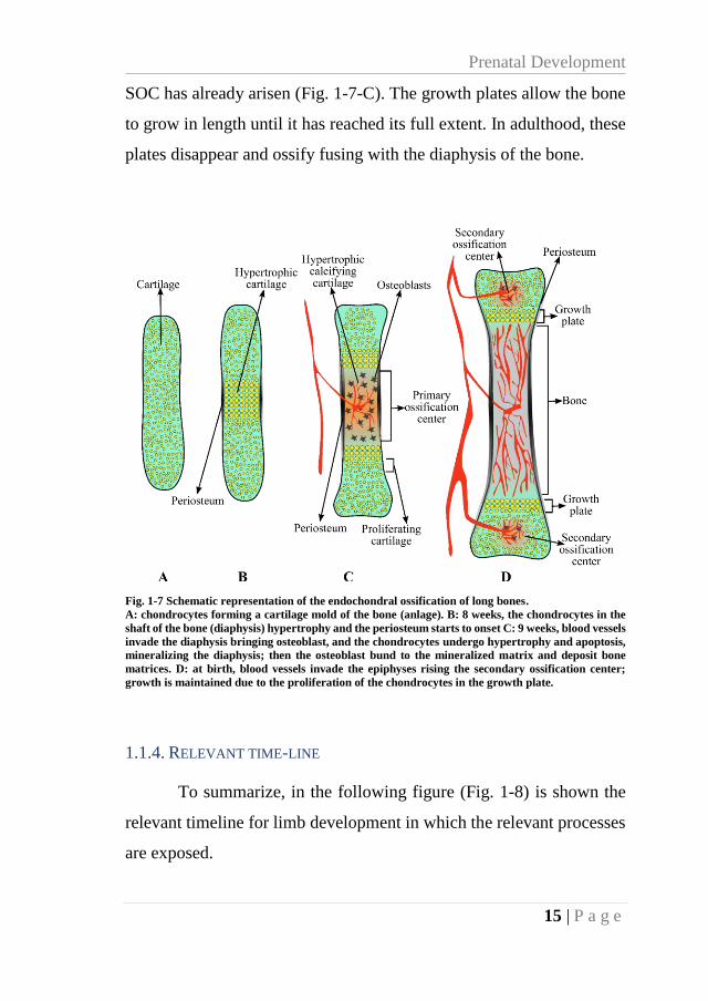
SOC has already arisen (Fig. 1-7-C). The growth plates allow the bone
to grow in length until it has reached its full extent. In adulthood, these
plates disappear and ossify fusing with the diaphysis of the bone.
Fig. 1-7 Schematic representation of the endochondral ossification of long bones.
A: chondrocytes forming a cartilage mold of the bone (anlage). B: 8 weeks, the chondrocytes in the
shaft of the bone (diaphysis) hypertrophy and the periosteum starts to onset C: 9 weeks, blood vessels
invade the diaphysis bringing osteoblast, and the chondrocytes undergo hypertrophy and apoptosis,
mineralizing the diaphysis; then the osteoblast bund to the mineralized matrix and deposit bone
matrices. D: at birth, blood vessels invade the epiphyses rising the secondary ossification center;
growth is maintained due to the proliferation of the chondrocytes in the growth plate.
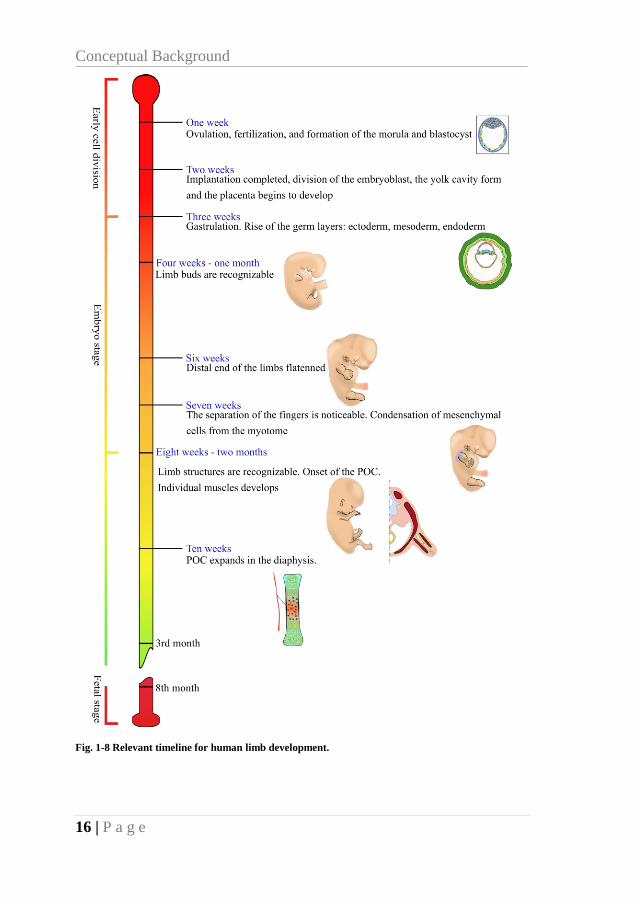
1.1.4. RELEVANT TIME-LINE
To summarize, in the following figure (Fig. 1-8) is shown the
relevant timeline for limb development in which the relevant processes
are exposed.
Conceptual Background
16 | P a g e
Fig. 1-8 Relevant timeline for human limb development.
Joints
17 | P a g e
1.2. JOINTS
Joints are the anatomical sites where two or more bones meet,
and their function is to allow a relative movement between bones
without losing the stability of the skeleton [24]. There are about 206
bones in the adult human body, and almost all of them are in contact
with at least one other bone. Therefore, the total number of joints can
be hundreds.
Joints are classified depending on both its structure and
function. Structural classification of joints is related to how the bones
are connected, while functional classification is used to describe the
relative movement between bones.
There are three main classes of joints when classified based on
their structure: the fibrous joints unite adjacent bones by fibrous
connective tissue; the cartilaginous joint connects bones through
hyaline cartilage or fibrocartilage; and the synovial joints do not
completely connect articulating bones, i.e., the articulating bony
surfaces are not in continuity as in the other types of joints. Instead, in
the synovial joints, the articulating surfaces are covered by hyaline
cartilage with limited contact between them and a very low coefficient
of friction, making the relative movement between them quite easy.
Additionally, in the synovial joints, there is a fibrous capsule that
surrounds the linked bones, the synovial capsule, that is filled with a
lubricant fluid, the synovial fluid, that helps to smooth the relative
movement between the bones.
Conceptual Background
18 | P a g e
On the other hand, joints are functionally classified as
synarthrosis (low mobility), amphiarthrosis (slight mobility) and
diarthrosis (free mobility). Fibrous and cartilaginous joints can be
classified to either synarthrosis or amphiarthrosis, whereas synovial
joints are always classified as diarthrosis.
The main function of the synarthroses is to provide a strong
union between the articulating bones, hence, this kind of joints are
mostly located in places where bones should protect internal organs
[24]. Among examples of this type of joints are included the bones of
the skull (fibrous joints), and the manubriosternal joint (cartilaginous
joint).
In amphiarthroses, the bones are connected by either an
interosseous ligament (fibrous joint) or by a disk of fibrocartilage
(cartilaginous joint) [24]. The function of these joints is both for
protection and to bring slight mobility between the involved bones.
Examples of these joints are the intervertebral joints (cartilaginous
joint), the pubic symphysis of the pelvis (cartilaginous joint), the joints
between ribs and sternum (cartilaginous joint), and the syndesmosis
joints (fibrous joints).
Diarthroses joints are highly movable joints in which the shapes
of the opposing cartilaginous surfaces are relatively congruent and
encircled within a synovial capsule filled with synovial fluid (all
synovial joints). Examples of these are included the hip, knee, shoulder,
elbow, among others.
Joints
19 | P a g e
1.2.1. SYNOVIAL JOINTS
Most synovial or diarthrotic joints are in the appendicular
skeleton (limbs), therefore they give the limbs a large range of motion.
Moreover, depending on the axe of motion of each joint (degrees of
freedom), joints can be classified into three categories: uniaxial, biaxial
and multiaxial. A uniaxial joint allows the relative motion between
bones only around one axis, such as the elbow. A biaxial joint allows
motion in two planes or around two axes, such as the
metacarpophalangeal. And finally, joints such as the shoulder or the hip
are considered as multiaxial, since they allow movement in several
directions (posterior-anterior, lateral-medial and around their long
axis).
Further classification of the synovial joints is related to their
articulating surfaces shapes. There are six types of joint within this
classification: pivot, hinge, condyloid, saddle, plane, and ball-and-
socket joints.
Pivot joints allow one bone to rotate on its axis, such as the
proximal radioulnar joint, where the head of the radius is largely
encircled by a ligament as it articulates with the radial notch of the ulna.
Functionally, this type of joint is classified as uniaxial joint.
The hinge joint only allows two kinds of motion (bending and
straightening) along a single axis, such as an interphalangeal joint.
Thus, hinge joints are functionally classified as uniaxial joints.
The condyloid or ellipsoidal joints have a shallow depression at
the end of one of the bones that articulate with a rounded structure from
Conceptual Background
20 | P a g e
adjacent bones. They can be found between the radius and carpal bones
or between the distal end of a metacarpal bone and the proximal
phalanx. Functionally, condyloid joints are biaxial joints that allow for
two planes of movement.
In saddle joints, the articulating surfaces present a saddle shape,
like a seat on a horse, but convex on one bone and concave in the other.
They can be found in the articulation between the trapezium carpal bone
and the first metacarpal bone (base of the thumb), providing the thumb
with the ability to move in two planes (parallel and perpendicular to the
palm). This movement of the joint is what gives the humans their
characteristic opposable thumbs [24]. These joints are functionally
classified as biaxial joints.
In plane joints, the articulating surfaces are flat so the bones can
slide against each other. Plane joints can be found between the carpal
bones (intercarpal joints) of the wrist or the tarsal bones (intertarsal
joints) of the foot, between the clavicle and acromion of the scapula
(acromioclavicular joint), and between the superior and inferior
articular processes of adjacent vertebrae (zygapophysial joints).
Regarding their functionality classification, because of their shape,
these joints can be described as multiaxial joints. However, depending
on the ligaments and neighbor bones, their movement could be limited.
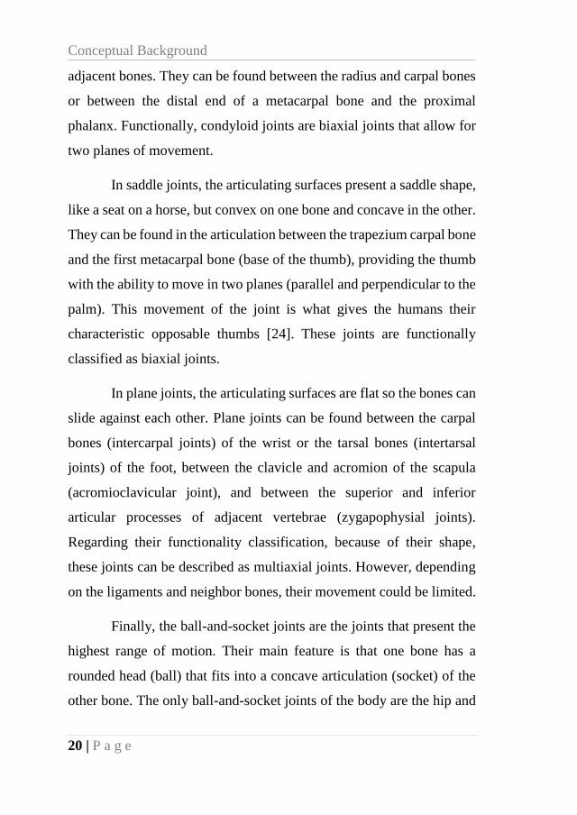
Finally, the ball-and-socket joints are the joints that present the
highest range of motion. Their main feature is that one bone has a
rounded head (ball) that fits into a concave articulation (socket) of the
other bone. The only ball-and-socket joints of the body are the hip and
Joints
21 | P a g e
the glenohumeral (shoulder). Ball-and-socket joints are functionally
classified as multiaxial joints.
1.2.2. SYNOVIAL JOINTS STRUCTURE
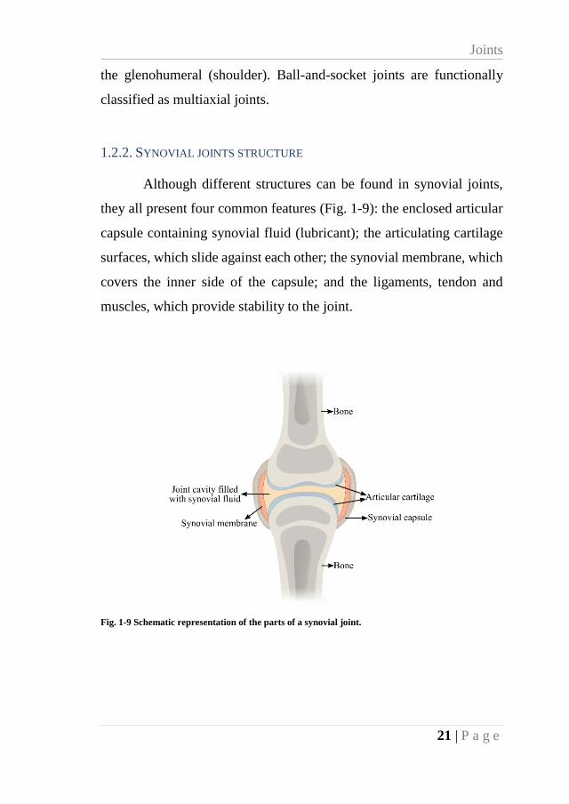
Although different structures can be found in synovial joints,
they all present four common features (Fig. 1-9): the enclosed articular
capsule containing synovial fluid (lubricant); the articulating cartilage
surfaces, which slide against each other; the synovial membrane, which
covers the inner side of the capsule; and the ligaments, tendon and
muscles, which provide stability to the joint.
Fig. 1-9 Schematic representation of the parts of a synovial joint.

Conceptual Background
22 | P a g e
1.2.3. ARTICULAR CARTILAGE
The cartilage is a specialized form of connective tissue, made-
up by chondrocytes. The chondrocytes are cells isolated in small spaces
of the extracellular matrix (ECM), composed by type II collagen fibers
embedded within a ground substance, i.e., colloidal gel full of water.
The cartilage is a non-vascularized tissue so the cells get nutrients from
the ground substance and its self-repairing capabilities are very limited
[25]. There are three types of cartilage: elastic, fibrous, and hyaline.
The elastic cartilage, as the name describes, is the most elastic
of the three. It can be found in the epiglottis, in the external ear and in
the walls of the ear conduct and the Eustachian tubes. Its extracellular
matrix is rich in both elastic fibers and collagen type II fibers.
The fibrous cartilage can be seen as a transition between dense
connective tissue and hyaline cartilage since it is made up of a
combination of dense collagen fibers (type I) and chondrocytes within
lacunae surrounded by hyaline matrix [25]. This type of cartilage can
be found in the intervertebral disks, the meniscus and, sometimes, in
the ligaments and tendons insertion sites.
The hyaline cartilage is the most abundant in the human body.
It covers the articulating bone ends in synovial joints, forming the
articular cartilage, a surface that helps to the force transmission and
distribution. The thickness of the articular cartilage varies from joint to
joint, but in humans is usually between 2-4 mm [26]. It can be described
as a poroelastic tissue, in which cells (chondrocytes) are embedded
within an ECM composed by a network of collagen fibers and
Joints
23 | P a g e
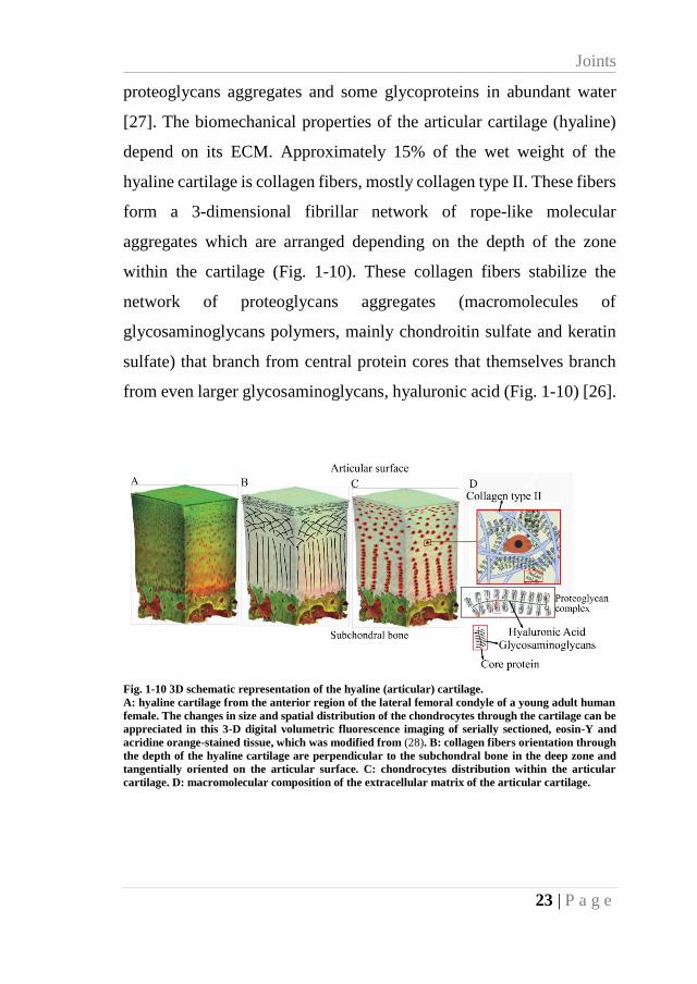
proteoglycans aggregates and some glycoproteins in abundant water
[27]. The biomechanical properties of the articular cartilage (hyaline)
depend on its ECM. Approximately 15% of the wet weight of the
hyaline cartilage is collagen fibers, mostly collagen type II. These fibers
form a 3-dimensional fibrillar network of rope-like molecular
aggregates which are arranged depending on the depth of the zone
within the cartilage (Fig. 1-10). These collagen fibers stabilize the
network of proteoglycans aggregates (macromolecules of
glycosaminoglycans polymers, mainly chondroitin sulfate and keratin
sulfate) that branch from central protein cores that themselves branch
from even larger glycosaminoglycans, hyaluronic acid (Fig. 1-10) [26].
Fig. 1-10 3D schematic representation of the hyaline (articular) cartilage.
A: hyaline cartilage from the anterior region of the lateral femoral condyle of a young adult human
female. The changes in size and spatial distribution of the chondrocytes through the cartilage can be
appreciated in this 3-D digital volumetric fluorescence imaging of serially sectioned, eosin-Y and
acridine orange-stained tissue, which was modified from (28). B: collagen fibers orientation through
the depth of the hyaline cartilage are perpendicular to the subchondral bone in the deep zone and
tangentially oriented on the articular surface. C: chondrocytes distribution within the articular
cartilage. D: macromolecular composition of the extracellular matrix of the articular cartilage.
Conceptual Background
24 | P a g e
The hyaline cartilage is maintained by the chondrocytes, which
are in charge of the production of the ECM material, so they oversee
the growth and repair of cartilage tissue. Moreover, the volume of the
chondrocytes in cartilage is less than 10% of the total cartilage volume,
and this percentage reduces with age [27].
1.2.4. CARTILAGE DISEASES
There are more than 100 pathologies of synovial joints,
specifically for the articular cartilage. What is more discouraging is that
all these pathologies do not share common pathways, and furthermore,
some of them are still not fully understood [26]. Nevertheless, each
arthritic disease usually targets a group of joints so it can be related to
a joint function or articular structure. Among all the pathologies the
most common diseases are OA, rheumatoid arthritis (RA) and gout
[26].
OA is a degenerative joint disease caused by the wearing and
degeneration of the hyaline cartilage due to multiple injuries to the joint
surface, aging, repeated trauma, surgery, obesity, and hormonal
disorders. This degeneration might cause the eventual loss of a portion
of the articular cartilage or the entire joint surface, which is worsened
by the poor ability of self-regeneration of the hyaline cartilage. In fact,
sometimes this cartilage degeneration causes that bones rub against
each other, generating pain [27]. Then, the bones thicken and from bony
spurs which can break off into the joint irritating soft tissues, producing
joint stiffness. Moreover, the synovial capsule becomes inflamed
causing more pain and, due to the inflammation, it generates cytokines
Joints
25 | P a g e
and enzymes that may damage the cartilage even more. Usually, the
cartilage tends to remodel itself through the replacement of worn
cartilage by a tougher tissue (fibrous cartilage), generating an uneven
articular surface, which can also cause pain and joint stiffness [26].
OA progresses through four stages [28]. In Grade I, the surface
and subsurface damage is minor, only small fissures and pits at points
of high stress of the joint. In Grade II, more damage can be seen at the
surface of the cartilage, however, still confined at the areas of high
stress. In Grade III, there is a complete loss of cartilage at the zones of
high stress, and probably there are formations of bony spurs. At this
stage is when the patient starts to feel pain. In Grade IV large areas of
bone might be exposed and the articular surface becomes irregular.
Currently, OA cannot be fully healed. However, when
diagnosed on the first stages, a modification in the lifestyle (weight loss,
nutritional supplements, physical therapy, and other strategies) can
reduce the disease advance velocity and relive pain. The problem is that
it is difficult to diagnose OA at an early stage because the joint pain and
stiffness usually appear in the later stages (Grade III and IV), when can
be too late. When nothing else works, surgery (joint replacement) is the
last approach for treating OA. Total joint replacement (TJR) or
arthroplasty is a surgical procedure that removes affected parts (both
articular surfaces) of the joint and replaces them with an artificial
equivalent. In the partial joint replacement, only one of the articular
surfaces is replaced with a replica.
On the other hand, RA is an autoimmune disorder in which the
immune system attacks, mistakenly, the healthy synovium.

Conceptual Background
26 | P a g e
Consequently, the production of synovial fluid is retarded and therefore
there is an inflammation of the joint cavity and neighbor tissue, which
eventually may contribute to damage joint tissue, including the
cartilage. The common symptoms, which can come and go, include
chronic pain, and joint stiffness and swelling. In contrast to OA, RA
affects small joints symmetrically.
Gout is a metabolism disorder in which final metabolite, uric
acid, crystallizes and precipitates in the synovial joint and neighbor
tissues. The high concentration of uric acid within the joint increases
the inflammatory response of the immune system. Among the
symptoms of gout are included a red, tender and swollen joint with pain.
1.2.5.SUBCHONDRAL BONE
The subchondral bone is the layer of bone just under the
cartilage; chondral refers to cartilage, while the prefix sub means
beneath. The subchondral bone remains connected to the articular
cartilage through the calcified cartilage and varies its architecture and
physiology by region [29]. The subchondral bone is composed by two
layers, the subchondral bone plate, under the calcified cartilage, and the
subchondral trabecular bone, which is closer to the medullary cavity
[29,30]. The subchondral bone plate has similar characteristics of the
compact (cortical) bone and its thickness ranges from 10𝜇𝑚 to 3mm
[29,30]. The subchondral bone is formed via endochondral ossification
of the of the cartilaginous structure on the epiphyses of the bone [30].
The function of the subchondral bone is that of shock absorber by
attenuating forces generated by locomotion. The compact subchondral
Joints
27 | P a g e
bone plate provides support, and the subchondral trabecular component
provides elasticity for shock absorption [29].
The subchondral bone matrix is a biphasic material which
includes organic and inorganic matrices. Up to 88% of the organic
matrix is collagen type I, the other 12% is made of the dry weight of
osteocalcin, osteonectin, phosphoproteins, lipids and proteoglycans
[30]. The inorganic component of the subchondral bone is mainly
hydroxyapatite crystals, which supply rigidity [29]. This unique
composition of the subchondral bone is designed to help with the
dispersion of loads across the joint [29].
The subchondral trabecular bone and the inner side of the
subchondral bone plate are covered by osteoblasts and osteoclasts
which allows the subchondral bone to adapt its morphology in response
to stresses. This adaptation follows Wolff’s Law, which states that bone
will adapt in response to the loading under which it is subjected [29,31].
The osteoblasts and osteoclasts facilitate the adaptive response through
apposition and resorption activities, respectively [29].
The rich vascularization and innervation of subchondral bone
facilitates the local response to both physiologic and pathologic events
[29]. Physiologically, the subchondral trabecular bone might provide an
additional source of cartilage nutrition in addition to the synovial fluid
[30]. On the other hand, the bone marrow of the subchondral trabecular
bone maintains a heterogenous population of multi-potent
mesenchymal cells which provide progenitor cells for differentiation of
osteochondral or any other cell lineage [30].
Conceptual Background
28 | P a g e
The subchondral bone is also affected by the OA, although it is
yet unclear if the pathological changes within the subchondral bone
precede the changes in the articular cartilage, or if the subchondral bone
changes are consequence of the bone adaptation that follows the
alterations in the biochemical and mechanical properties of the cartilage
[32]. In early stages of OA, it can be noticed an increase in thickness of
the subchondral bone plate as well as of the underlying trabeculae. In
later stages, the subchondral bone goes through remodeling processes,
especially in areas where the overlaying articular cartilage has suffered
advanced destruction [32]. In advanced stages of OA, besides the
extensive bone sclerosis, the bone can also suffer necrosis, and in areas
of total cartilage destruction, the synovial fluid gets access to the bone
marrow inducing changes of the mesenchymal cells [32]. This leads to
cartilage-nodules within the subchondral bone. These changes in the
subchondral bone are responsible for the osteoarthritic joint pain [32].
1.3.FINITE ELEMENT METHOD (FEM)
In general, every phenomenon in nature can be described with
the aid of physics through equations relating quantities of interest. That
way, mathematics becomes an aid to understand and quantify any
physical phenomena such as structural or fluid behavior, stress
distribution in complex structures, thermal transport, aerodynamic
loads, the concentration of molecules, pollutants and other substances,
wave propagation, the growth of biological cells, weather predictions,
etc. Engineers and scientists have two major tasks when studying a
physical phenomenon: first, the mathematical formulation of the
Finite Element Method (FEM)
29 | P a g e
physical process; and second, numerical analysis. For the development
of the mathematical model of a process, some assumptions related to
how the process work needs to be made. It might be possible that the
formulation of the mathematical model is not that difficult; however,
the solution, numerical analysis, within a domain is a gigantic task. It is
here where approximate methods of analysis are valuable tools to find
approximate solutions to the mathematical model of our interest.
Most processes in nature can be described by using partial
differential equations (PDEs). However, to solve these equations for an
arbitrary shape through classical methods is nearly impossible.
Therefore, computational technics to solve large equations systems
have been developed in the last decades, among which the most
prominent and used is the FEM.
FEM is a numerical tool used to obtain approximated solutions
of a problem, which can be interpreted as a prediction of how the
process will develop under given conditions [33]. The base of FEM is:
“Divide and conquer!”
In FEM, the area of study (the domain of interest) has to be
divided into small finite elements, which can be just called elements,
connected by nodes. That way a finite element mesh of the analyzed
structure is obtained (Fig. 1-11). Thereafter, the PDEs are calculated in
every single element [33]. These calculations are done through
polynomial approximations, which are in fact interpolations over the
element. This denotes that the exact values at specific points within the
element are calculated, but not within the entire element. These specific
points are the abovementioned nodes (also called nodal points), which

Conceptual Background
30 | P a g e
often are at the boundary of the element and shared with neighbor
elements. All the individual elemental results are then combined to
obtain the final result of the entire domain of interest.
The accuracy with which the variable is calculated depends on
the type of approximation (interpolation) that is used, which can be
linear, quadratic, cubic, etc. Moreover, the accuracy of the solution can
also be improved if the number of elements, and therefore nodes,
increases [33]. However, the computational cost can escalate a lot with
the number of elements and the complexity of the considered
approximations. The results are usually presented as contour plots
giving information of how the variable is distributed at any given time
(Fig. 1-11).
Fig. 1-11 Schematic representation of a finite element mesh.
Left: finite elements of a domain of interest. Center: Zoom of a part of the mesh where an element
and surrounding nodes are specified. Right: the contour plot of the result of a variable within the
domain of interest.
31 | P a g e
Chapter 2. JOINT ONSET
2.1. INTRODUCTION
As previously mentioned, the joint formation occurs in the
embryonic stages of life and is critical to allow movement between
bones. The appendicular skeleton formation initiates with the
appearance of the limb bud, which has within it an uninterrupted and
uniform condensation of mesenchymal cells (skeletal blastema) [34,35]
(Fig. 2-1-A). Most blastemal cells differentiate into chondrocytes;
however, some of the blastemal cells remain undifferentiated at the site
of the future joint known as interzone (Fig. 2-1-B).
The definitive separation of the future bones of the joint occurs
with cavitation, which creates a space between chondrocyte rudiments,
that later will be occupied by synovial fluid (Fig. 2-1-C). Some studies
(in rats and avian embryos) have shown that cells in the middle of the
interzone display necrotic features which induce the separation of the
chondrocyte rudiments [36–38]. After cleavage, joint morphogenesis
occurs as cells proliferate on either side of the joint, and it takes its
shape (Fig. 2-1-D) [34,39]. This shape is influenced by movements and
muscle contractions that occur during limb development [21,40], as
well as by local and systemic biochemical factors [34].
Experimental models, in vivo and in vitro, have explored the
conditions in which abnormal environments affect the embryo
development and have provided insights about the molecules that play

Joint Onset
32 | P a g e
critical roles in joint formation [34,41–47]. In the initial stages of joint
development, Wnt is expressed to maintain the mesenchymal nature of
cells at the interzone [34,46,48,49]. Simultaneously, Growth
Differential Factor-5 (GDF-5) is also expressed playing a pivotal role
in joint development by marking the interzone site [50–52]. The GDF-
5 antagonists, chordin and noggin, are expressed in chondrocytes in the
developing rudiment. HOX genes may also play a role in defining
boundaries and the limb patterns in development [46]. After the onset
of the interzone, other molecules take lead of bone development; for
instance, Indian hedgehog signaling molecule (Ihh) and Parathyroid
Hormone-related Protein (PTHrP) control growth and differentiation to
regulate ossification and the final shape of the bones [53].
Results from in vivo experiments studying joint onset conditions
during embryo development are complemented by computational
studies. Computational models have analyzed the effect of muscle load
on the shape of the developing joint, both in 2D [20] and 3D [21].
However, these models do not describe the initial stages of joint
development (interzone onset and cavitation). Moreover, computational
models can also be used to understand the biochemical and molecular
behavior of the biological phenomenon of development. For instance,
the interactions of Ihh, PTHrP and Vascular Endothelial Growth Factor
(VEGF) in endochondral ossification have been studied in 1D finite
element model for the human-distal-femoral growth plate [54]. The
previous model was extended to a 2D simulation of bone growth during
the fetal stage and analyzed the shape in later stages [9]. These models
have been expanded to simulate cartilage hypertrophy (during bone

Introduction
33 | P a g e
growth) and onset of the secondary ossification center [9,55,56]. Also,
Garzón-Alvarado et al., presented a mathematical model of
chondrocyte hypertrophy, which was able to predict the onset of
secondary ossification centers of long bones, regulated by molecular
factors [13].
Fig. 2-1 Scheme of the stages of the synovial joints during the interphalangeal joint development.
A. Blastemal cells, which are mesenchymal cells condensed in the first stages of the limb; no joint
formation is observed. B. Interzone formation: it is composed by an aggrupation and condensation
of mesenchymal cells. Meanwhile, the mesenchymal cells that will form (future) bones condensate
and differentiate into chondrocytes cells, establishing an anlagen bones [34]. C. The cavitation
process initiates, and the formation of the synovial cavity takes place. D. Morphogenetic process
starts to mold the opposite surfaces of the joint, E. Finally, all joint components are developed,
including articular cartilage, joint capsule and synovial cavity.
Reaction-diffusion systems are often used as models for pattern
formation of a variety of structures during development [13,46,57].
Such tuned systems produce well-organized patterns called Turing
patterns, which result in definitive patterns of molecule distribution
Joint Onset
34 | P a g e
[46,57]. In an enzyme-substrate model (or depletion model as proposed
by Turing [58]), a stable spatial pattern forms after temporal evolution
[59]. The patterns of chemical gradients are influenced by the diffusion
rates, the growth rates, and the bounding geometry of the system [60].
In this work, we use reaction-diffusion equations and the formation of
Turing patterns to simulate the location of joint cleavage, the number
of joints formed and the condylar shape of the joint.
The aim of this work was to develop a computational model
based on two generic molecular actions (proliferation and growth) and
two regulatory loops, expressed as reaction-diffusion equations. The
aim was to predict the molecular patterns associated with the joint
formation process and the way in which it influences the final shape of
the joint. The model was solved in a finite elements’ framework.
Mathematical equations predicted patterns representing molecular
mechanisms that model the structures and shapes of joint development
such as interzone onset, cavitation, and condylar shape of the bones
ends of the joint.
2.2. MATERIALS AND METHODS
2.2.1. BIOLOGICAL ASPECTS CONSIDERED FOR THE JOINT DEVELOPMENT
MODEL
There are many biochemical factors influencing joint
development [34,61–64]. Advances in experimental techniques have
provided detailed information regarding geometry, processes timing,
and regulatory interactions [65]. However, the joint development
Materials and Methods
35 | P a g e
process is not entirely clear in the literature. Therefore, based on what
is reported, we modeled six generic molecular factors involved in joint
onset; each factor may represent multiple molecules achieving the same
action. The process in our model was organized into two stages; the first
stage marks the interzone onset, where high concentration of a molecule
(G) establish where the mesenchymal tissue will not differentiate into
chondral tissue (interzone). Afterwards, those zones that differentiate
into cartilage secrete (I) and (P) which establish a regulatory loop that
governs cell proliferation and hypertrophy, commencing bone growth
and ossification processes (second stage). Meanwhile, the domain
keeps growing and other molecules, (H) and (W), regulated the joint
separation and related structures.
We modeled two factors in demarcating the position of the joint:
a factor (G) which is in charge of locating the cleavage position and its
antagonist (N) is everywhere else. The factor (G) could represent GDF-
5, which belongs to the Bone Morphogenetic Protein (BMP) family and
promotes interzone tissue function, preventing the differentiation of the
mesenchymal tissue into cartilage [50–52]. Its antagonist could be the
BMP antagonist Noggin (N). Also, it is considered a factor regulating
cellular proliferation, termed growth (H), this molecule controls the
differential amount of growth in the tissue from proximal to distal. This
molecule could be relate to HOX genes [62–64], or any other molecule
related to bone limb bud growth. Mathematically, there is a gradient in
H, which affected the growth rate by promoting the longitudinal growth
of the limb and bone anlagen.
Joint Onset
36 | P a g e
Many studies have shown that after formation of the interzone,
cartilage behavior is governed by a negative feedback loop involving
Ihh and PTHrP [66]. We introduce a factor (I) that could represent Ihh,
which regulates chondrocyte proliferation, maturation, and hypertrophy
[66–69], and a factor (P), which could represent PTHrP and inhibits
chondrocyte hypertrophy [67]. Additionally, factor (W) was expressed
in the interzone, inducing cell death and allowing the creation of a joint
space. This factor represents Wnt/β-catenin signaling that leads to
separation of the rudiments [34,36,37,70] and is also observed in parts
of the fibrous capsule and the synovial lining of the joint capsule in later
stages of development [46,57].
The variables in our model represented concentrations of each
mentioned molecular factor (𝑆𝐺 , 𝑆𝑁, 𝑆𝐻, 𝑆𝐼 , 𝑆𝑃, 𝑆𝑊) and their diffusion
coefficients, 𝐷𝑖. Variables also included the growth rates based upon
the concentration S of each molecule. All these variables will feed a
finite element model with Partial Differential Equation integrated with
a Cellular Automaton-like system (PDE+CA-like), CA-like because it
was not based on any of the traditional CA models but can be explained
as one. The PDE describes the molecular diffusion and established the
biochemical concentrations, which enable the CA-like part to determine
whether the tissue differentiated or not. For this last part, each element
started with a tissue state (mesenchymal, pre-cartilaginous,
cartilaginous, interzone) and the CA-like system allowed the element to
“jump” (differentiate) from one tissue state to another, according to the
molecular concentration within each element. Additionally, each tissue
state was associated with a cell type and cell concentration.
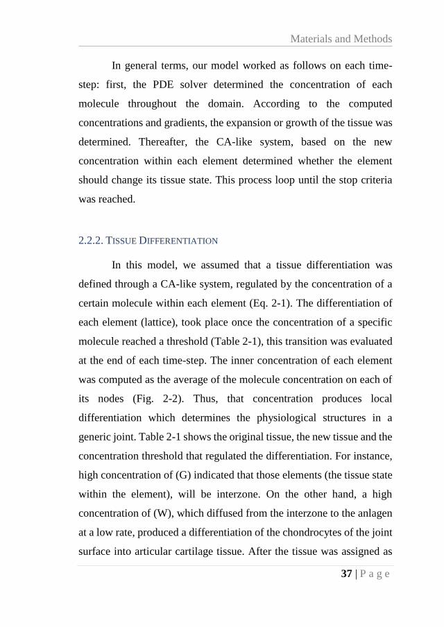
Materials and Methods
37 | P a g e
In general terms, our model worked as follows on each time-
step: first, the PDE solver determined the concentration of each
molecule throughout the domain. According to the computed
concentrations and gradients, the expansion or growth of the tissue was
determined. Thereafter, the CA-like system, based on the new
concentration within each element determined whether the element
should change its tissue state. This process loop until the stop criteria
was reached.
2.2.2. TISSUE DIFFERENTIATION
In this model, we assumed that a tissue differentiation was
defined through a CA-like system, regulated by the concentration of a
certain molecule within each element (Eq. 2-1). The differentiation of
each element (lattice), took place once the concentration of a specific
molecule reached a threshold (Table 2-1), this transition was evaluated
at the end of each time-step. The inner concentration of each element
was computed as the average of the molecule concentration on each of
its nodes (Fig. 2-2). Thus, that concentration produces local
differentiation which determines the physiological structures in a
generic joint. Table 2-1 shows the original tissue, the new tissue and the
concentration threshold that regulated the differentiation. For instance,
high concentration of (G) indicated that those elements (the tissue state
within the element), will be interzone. On the other hand, a high
concentration of (W), which diffused from the interzone to the anlagen
at a low rate, produced a differentiation of the chondrocytes of the joint
surface into articular cartilage tissue. After the tissue was assigned as
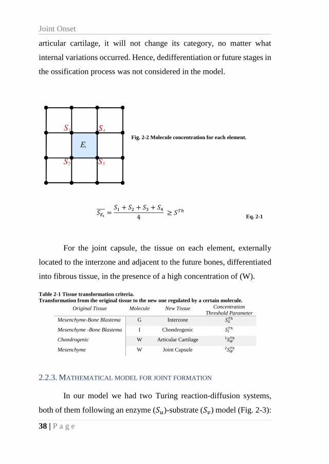
Joint Onset
38 | P a g e
articular cartilage, it will not change its category, no matter what
internal variations occurred. Hence, dedifferentiation or future stages in
the ossification process was not considered in the model.
Fig. 2-2 Molecule concentration for each element.
𝑆𝐸𝑖̅̅ ̅̅ =
𝑆1 + 𝑆2 + 𝑆3 + 𝑆44
≥ 𝑆𝑇ℎ Eq. 2-1
For the joint capsule, the tissue on each element, externally
located to the interzone and adjacent to the future bones, differentiated
into fibrous tissue, in the presence of a high concentration of (W).
Table 2-1 Tissue transformation criteria.
Transformation from the original tissue to the new one regulated by a certain molecule.
Original Tissue Molecule New Tissue Concentration
Threshold Parameter
Mesenchyme-Bone Blastema G Interzone 𝑆𝐺𝑇ℎ
Mesenchyme -Bone Blastema I Chondrogenic 𝑆𝐼𝑇ℎ
Chondrogenic W Articular Cartilage 𝑆𝑊𝑇ℎ1
Mesenchyme W Joint Capsule 𝑆𝑊𝑇ℎ2
2.2.3. MATHEMATICAL MODEL FOR JOINT FORMATION
In our model we had two Turing reaction-diffusion systems,
both of them following an enzyme (𝑆𝑢)-substrate (𝑆𝑣) model (Fig. 2-3):
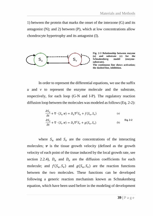
Materials and Methods
39 | P a g e
1) between the protein that marks the onset of the interzone (G) and its
antagonist (N); and 2) between (P), which at low concentrations allow
chondrocyte hypertrophy and its antagonist (I).
Fig. 2-3 Relationship between enzyme
(u) and substrate (v) for the
Schnakenberg model (enzyme-
substrate).
The continuous line shows activation;
the dashed line, inhibition.
In order to represent the differential equations, we use the suffix
u and v to represent the enzyme molecule and the substrate,
respectively, for each loop (G-N and I-P). The regulatory reaction
diffusion loop between the molecules was modeled as follows (Eq. 2-2):
𝜕𝑆𝑢𝜕𝑡
+ ∇ ∙ (𝑆𝑢 𝒗) = 𝐷𝑢∇2𝑆𝑢 + 𝑓(𝑆𝑢 , 𝑆𝑣) (a)
Eq. 2-2 𝜕𝑆𝑣𝜕𝑡
+ ∇ ∙ (𝑆𝑣 𝒗) = 𝐷𝑣∇2𝑆𝑣 + 𝑔(𝑆𝑢 , 𝑆𝑣) (b)
where 𝑆𝑢 and 𝑆𝑣 are the concentrations of the interacting
molecules; 𝒗 is the tissue growth velocity (defined as the growth
velocity of each point of the tissue induced by the local growth rate, see
section 2.2.4), 𝐷𝑢 and 𝐷𝑣 are the diffusion coefficients for each
molecule; and 𝑓(𝑆𝑢, 𝑆𝑣) and 𝑔(𝑆𝑢, 𝑆𝑣) are the reaction functions
between the two molecules. These functions can be developed
following a generic reaction mechanism known as Schnakenberg
equation, which have been used before in the modeling of development
Joint Onset
40 | P a g e
process and can produce several patterns similar to those found in
nature [9,71–73] (Eq. 2-3 and Eq. 2-4):
𝑓(𝑆𝑢 , 𝑆𝑣) = 𝛾𝐶𝑐𝑒𝑙𝑙(𝑎 − 𝑆𝑢 + 𝑆𝑢2𝑆𝑣)
Eq. 2-3
𝑔(𝑆𝑢 , 𝑆𝑣) = 𝛾𝐶𝑐𝑒𝑙𝑙(𝑏 − 𝑆𝑢2𝑆𝑣)
Eq. 2-4
where γ is a factor that takes into account the expression rate of
each molecule; Ccell is the concentration of cells that express molecules.
In our model, mesenchymal cells (CM), which are associated with
mesenchymal tissue, express the factors G and N, and pre-cartilage cells
(CC) which are associated with cartilage tissue, express factor I and P.
Ccell had a value of one or zero, depending on the cell type, therefore
this term acted as switch depending on the tissue type; for instance,
(CC = 0) if the tissue was mesenchymal, and (CC = 1) if the tissue was
pre-cartilage, whereas (CM = 0) if the cells are pre-cartilaginous, and
(CM = 1) if the cells are mesenchymal. The constants a and b are source
terms of each molecule involved in the loop. These equations establish
a nonlinear interaction between the molecules u and 𝑣: in presence of
𝑣, 𝑢 is upregulated, while in presence of 𝑢, 𝑣 is downregulated [46,57]
(Fig. 2-3). The reaction term interacts with the diffusion and produces
patterns that emerge when certain requirements are fulfilled. Turing
considered an interacting system which steady state would be driven
unstable by diffusion [46,57]. Each reaction-diffusion system, in order
to guarantee the Turing instability to occur, should satisfy the following
statements (Eq. 2-5, Eq. 2-6 and Eq. 2-7). The conditions for instability
could give us information about the presence (or not) of the Turing
patterns [74]:
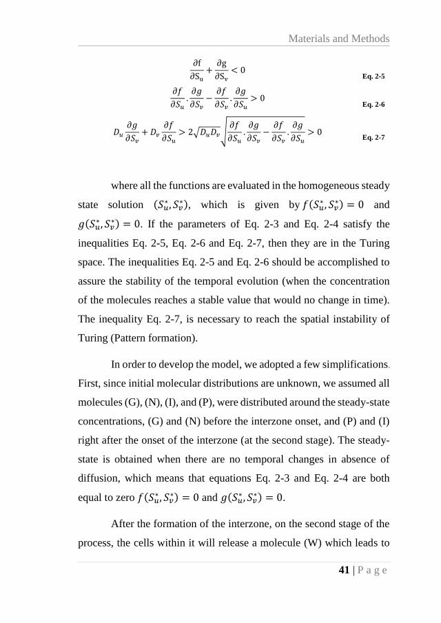
Materials and Methods
41 | P a g e
∂f
∂Su+∂g
∂Sv< 0
Eq. 2-5
𝜕𝑓
𝜕𝑆𝑢.𝜕𝑔
𝜕𝑆𝑣−𝜕𝑓
𝜕𝑆𝑣.𝜕𝑔
𝜕𝑆𝑢> 0
Eq. 2-6
𝐷𝑢𝜕𝑔
𝜕𝑆𝑣+ 𝐷𝑣
𝜕𝑓
𝜕𝑆𝑢> 2√𝐷𝑢𝐷𝑣√
𝜕𝑓
𝜕𝑆𝑢.𝜕𝑔
𝜕𝑆𝑣−𝜕𝑓
𝜕𝑆𝑣.𝜕𝑔
𝜕𝑆𝑢> 0
Eq. 2-7
where all the functions are evaluated in the homogeneous steady
state solution (𝑆𝑢∗ , 𝑆𝑣
∗), which is given by 𝑓(𝑆𝑢∗ , 𝑆𝑣
∗) = 0 and
𝑔(𝑆𝑢∗ , 𝑆𝑣
∗) = 0. If the parameters of Eq. 2-3 and Eq. 2-4 satisfy the
inequalities Eq. 2-5, Eq. 2-6 and Eq. 2-7, then they are in the Turing
space. The inequalities Eq. 2-5 and Eq. 2-6 should be accomplished to
assure the stability of the temporal evolution (when the concentration
of the molecules reaches a stable value that would no change in time).
The inequality Eq. 2-7, is necessary to reach the spatial instability of
Turing (Pattern formation).
In order to develop the model, we adopted a few simplifications.
First, since initial molecular distributions are unknown, we assumed all
molecules (G), (N), (I), and (P), were distributed around the steady-state
concentrations, (G) and (N) before the interzone onset, and (P) and (I)
right after the onset of the interzone (at the second stage). The steady-
state is obtained when there are no temporal changes in absence of
diffusion, which means that equations Eq. 2-3 and Eq. 2-4 are both
equal to zero 𝑓(𝑆𝑢∗ , 𝑆𝑣
∗) = 0 and 𝑔(𝑆𝑢∗ , 𝑆𝑣
∗) = 0.
After the formation of the interzone, on the second stage of the
process, the cells within it will release a molecule (W) which leads to
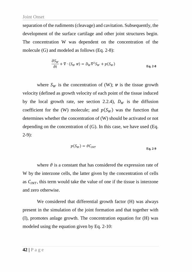
Joint Onset
42 | P a g e
separation of the rudiments (cleavage) and cavitation. Subsequently, the
development of the surface cartilage and other joint structures begin.
The concentration W was dependent on the concentration of the
molecule (G) and modeled as follows (Eq. 2-8):
𝜕𝑆𝑊𝜕𝑡
+ ∇ ∙ (𝑆𝑊 𝒗) = 𝐷𝑊∇2𝑆𝑊 + 𝑝(𝑆𝑊) Eq. 2-8
where 𝑆𝑊 is the concentration of (W); 𝒗 is the tissue growth
velocity (defined as growth velocity of each point of the tissue induced
by the local growth rate, see section 2.2.4), 𝐷𝑊 is the diffusion
coefficient for the (W) molecule; and 𝑝(𝑆𝑊) was the function that
determines whether the concentration of (W) should be activated or not
depending on the concentration of (G). In this case, we have used (Eq.
2-9):
𝑝(𝑆𝑊) = 𝜗𝐶𝐼𝑁𝑇 Eq. 2-9
where 𝜗 is a constant that has considered the expression rate of
W by the interzone cells, the latter given by the concentration of cells
as 𝐶𝐼𝑁𝑇, this term would take the value of one if the tissue is interzone
and zero otherwise.
We considered that differential growth factor (H) was always
present in the simulation of the joint formation and that together with
(I), promotes anlage growth. The concentration equation for (H) was
modeled using the equation given by Eq. 2-10:
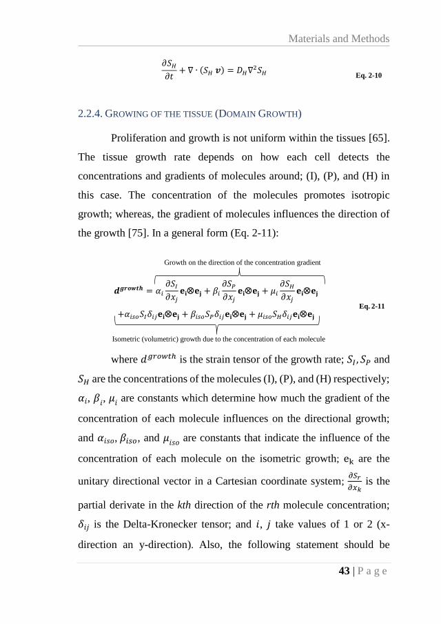
Materials and Methods
43 | P a g e
𝜕𝑆𝐻𝜕𝑡
+ ∇ ∙ (𝑆𝐻 𝒗) = 𝐷𝐻∇2𝑆𝐻
Eq. 2-10
2.2.4. GROWING OF THE TISSUE (DOMAIN GROWTH)
Proliferation and growth is not uniform within the tissues [65].
The tissue growth rate depends on how each cell detects the
concentrations and gradients of molecules around; (I), (P), and (H) in
this case. The concentration of the molecules promotes isotropic
growth; whereas, the gradient of molecules influences the direction of
the growth [75]. In a general form (Eq. 2-11):
𝒅𝒈𝒓𝒐𝒘𝒕𝒉 = 𝛼𝑖∂𝑆𝐼𝜕𝑥𝑗
𝐞𝐢𝐞𝐣 + 𝛽𝑖∂𝑆𝑃𝜕𝑥𝑗
𝐞𝐢𝐞𝐣 + 𝜇𝑖∂𝑆𝐻𝜕𝑥𝑗
𝐞𝐢𝐞𝐣
+𝛼𝑖𝑠𝑜𝑆𝐼𝛿𝑖𝑗𝐞𝐢𝐞𝐣 + 𝛽𝑖𝑠𝑜𝑆𝑃𝛿𝑖𝑗𝐞𝐢𝐞𝐣 + 𝜇𝑖𝑠𝑜𝑆𝐻𝛿𝑖𝑗𝐞𝐢𝐞𝐣 Eq. 2-11
where 𝑑𝑔𝑟𝑜𝑤𝑡ℎ is the strain tensor of the growth rate; 𝑆𝐼 , 𝑆𝑃 and
𝑆𝐻 are the concentrations of the molecules (I), (P), and (H) respectively;
𝛼𝑖, 𝛽𝑖, 𝜇𝑖 are constants which determine how much the gradient of the
concentration of each molecule influences on the directional growth;
and 𝛼𝑖𝑠𝑜, 𝛽𝑖𝑠𝑜, and 𝜇𝑖𝑠𝑜 are constants that indicate the influence of the
concentration of each molecule on the isometric growth; ek are the
unitary directional vector in a Cartesian coordinate system; ∂𝑆𝑟
𝜕𝑥𝑘 is the
partial derivate in the kth direction of the rth molecule concentration;
𝛿𝑖𝑗 is the Delta-Kronecker tensor; and 𝑖, 𝑗 take values of 1 or 2 (x-
direction an y-direction). Also, the following statement should be
Growth on the direction of the concentration gradient
Isometric (volumetric) growth due to the concentration of each molecule
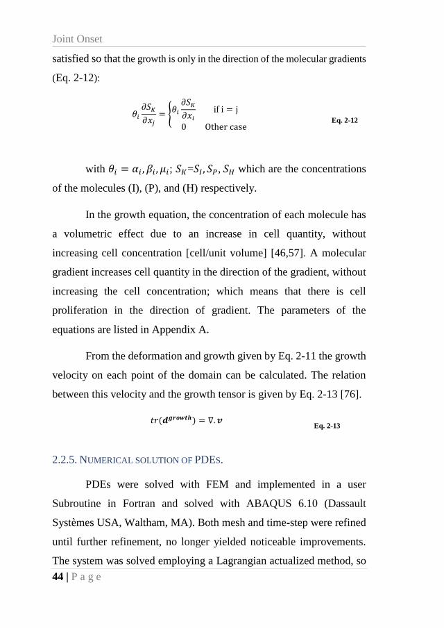
Joint Onset
44 | P a g e
satisfied so that the growth is only in the direction of the molecular gradients
(Eq. 2-12):
𝜃𝑖∂𝑆𝐾𝜕𝑥𝑗
= {𝜃𝑖∂𝑆𝐾𝜕𝑥𝑖
if i = j
0 Other case
Eq. 2-12
with 𝜃𝑖 = 𝛼𝑖 , 𝛽𝑖, 𝜇𝑖; 𝑆𝐾=𝑆𝐼 , 𝑆𝑃, 𝑆𝐻 which are the concentrations
of the molecules (I), (P), and (H) respectively.
In the growth equation, the concentration of each molecule has
a volumetric effect due to an increase in cell quantity, without
increasing cell concentration [cell/unit volume] [46,57]. A molecular
gradient increases cell quantity in the direction of the gradient, without
increasing the cell concentration; which means that there is cell
proliferation in the direction of gradient. The parameters of the
equations are listed in Appendix A.
From the deformation and growth given by Eq. 2-11 the growth
velocity on each point of the domain can be calculated. The relation
between this velocity and the growth tensor is given by Eq. 2-13 [76].
𝑡𝑟(𝒅𝒈𝒓𝒐𝒘𝒕𝒉) = ∇. 𝒗 Eq. 2-13
2.2.5. NUMERICAL SOLUTION OF PDES.
PDEs were solved with FEM and implemented in a user
Subroutine in Fortran and solved with ABAQUS 6.10 (Dassault
Systèmes USA, Waltham, MA). Both mesh and time-step were refined
until further refinement, no longer yielded noticeable improvements.
The system was solved employing a Lagrangian actualized method, so
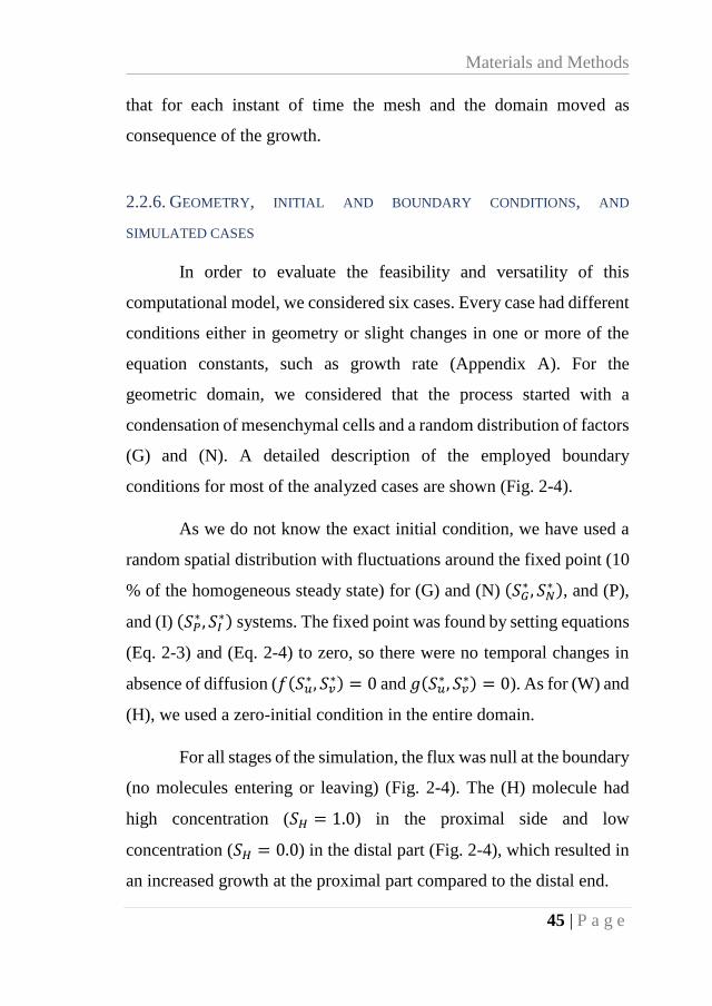
Materials and Methods
45 | P a g e
that for each instant of time the mesh and the domain moved as
consequence of the growth.
2.2.6. GEOMETRY, INITIAL AND BOUNDARY CONDITIONS, AND
SIMULATED CASES
In order to evaluate the feasibility and versatility of this
computational model, we considered six cases. Every case had different
conditions either in geometry or slight changes in one or more of the
equation constants, such as growth rate (Appendix A). For the
geometric domain, we considered that the process started with a
condensation of mesenchymal cells and a random distribution of factors
(G) and (N). A detailed description of the employed boundary
conditions for most of the analyzed cases are shown (Fig. 2-4).
As we do not know the exact initial condition, we have used a
random spatial distribution with fluctuations around the fixed point (10
% of the homogeneous steady state) for (G) and (N) (𝑆𝐺∗ , 𝑆𝑁
∗ ), and (P),
and (I) (𝑆𝑃∗ , 𝑆𝐼
∗) systems. The fixed point was found by setting equations
(Eq. 2-3) and (Eq. 2-4) to zero, so there were no temporal changes in
absence of diffusion (𝑓(𝑆𝑢∗ , 𝑆𝑣
∗) = 0 and 𝑔(𝑆𝑢∗ , 𝑆𝑣
∗) = 0). As for (W) and
(H), we used a zero-initial condition in the entire domain.
For all stages of the simulation, the flux was null at the boundary
(no molecules entering or leaving) (Fig. 2-4). The (H) molecule had
high concentration (𝑆𝐻 = 1.0) in the proximal side and low
concentration (𝑆𝐻 = 0.0) in the distal part (Fig. 2-4), which resulted in
an increased growth at the proximal part compared to the distal end.
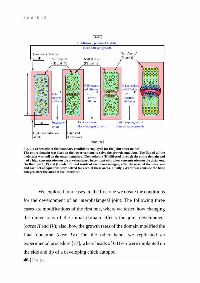
Joint Onset
46 | P a g e
Fig. 2-4 Schematic of the boundary conditions employed for the joint onset model.
The entire domain was fixed in the lower contour to solve the growth equations. The flux of all the
molecules was null on the outer boundary. The molecule (H) diffused through the entire domain and
had a high concentration on the proximal part, in contrast with a low concentration on the distal one.
On their part, (P) and (I) only diffused inside of each bone anlagen, after the onset of the interzone
and each set of equations were solved for each of these areas. Finally, (W) diffuses outside the bone
anlagen after the onset of the interzone.
We explored four cases. In the first one we create the conditions
for the development of an interphalangeal joint. The following three
cases are modifications of the first one, where we tested how changing
the dimensions of the initial domain affects the joint development
(cases II and IV); also, how the growth rates of the domain modified the
final outcome (case IV). On the other hand, we replicated an
experimental procedure [77], where beads of GDF-5 were implanted on
the side and tip of a developing chick autopod.

Results
47 | P a g e
2.3. RESULTS
2.3.1. CASE I: INTERPHALANGEAL JOINT DEVELOPMENT
In the case I, the limb bud had a length/width ratio of 3, based
on histology of the phalange anlage [78]. In the first stage (G-N
reaction-diffusion), we obtained the spatial distributions of (G) and (N)
over time, that indicated the formation of a stable Turing pattern (Fig.
2-5). The region where (G) was high indicated the interzone onset
(shown with an ‘*’) and location for cavitation.
In the second stage (P-I reaction), (P) accumulated in the distal
part of the bones, where it kept the proliferative state of the chondrocyte
cells (Fig. 2-5). (I) was inhibited when there was a high concentration
of (P), and in the zones of high (I) the hypertrophy was accelerated.
Also, the growth of the tissue was influenced by the concentration and
gradient of the molecules (I), (P), and (H) according to the equation (Eq.
2-11). In regions with a high concentration of (I) and low concentration
of (P), which caused hypertrophy of the cells, an epiphysis-like
structure was be obtained, wider than the rest of the bone (Fig. 2-5).
After the onset of the interzone, (W) started diffusing. (W) was
expressed in the interzone and where the fibrous capsule and the
synovial lining of the joint capsule will form (Fig. 2-5). Thus, we
obtained a hinge-like joint structure, which was similar in shape to an
interphalangeal joint. The distal bone had a wider proximal end and the
proximal one was uniform in width (Fig. 2-5).
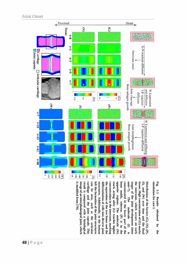
Joint Onset
48 | P a g e
Fig
. 2
-5
Resu
lts o
bta
ined
b
y
the
simu
latio
n fo
r ca
se I.
Distr
ibu
tion
of th
e facto
rs (G
), (N), (P
),
(I), a
nd
(W
) ov
er
time
an
d
the
final
tissue. H
igh
con
cen
tratio
n o
f (G) m
ark
s
the
inter
zon
e,
wh
ich
occu
rs
on
ea
rly
stages
of
the
join
t d
evelo
pm
en
t (tim
e
un
it=7
). T
he
mole
cu
le
(I) is
co
nce
ntra
ted
in
th
e lo
wer p
art
of
the
bo
ne
mold
s, w
her
eas
(P)
is in
th
e
op
po
site
regio
ns.
Th
e
molec
ule
(W)
starts
actin
g a
fter (G
) rea
ch
es h
igh
er
co
nce
ntra
tion
in th
e inter
zon
e, m
ark
ing
the sep
ara
tion
of th
e tw
o b
on
es a
nd
the
diffe
ren
tiatio
n o
f cells in
to d
iverse
join
t
stru
ctu
res. A
dd
ition
ally
, in th
e b
otto
m
left th
e form
atio
n o
f the jo
int str
uctu
res
ca
n
be
seen
, su
ch
a
s th
e a
rticu
lar
ca
rtila
ge
an
d
the
join
t ca
psu
le.
Th
is
resu
lt is
com
pared
w
ith a h
istolo
gic
al
ima
ge o
f an
inte
rp
ha
lan
gea
l join
t, wh
ich
is mo
difie
d fr
om
[79
].
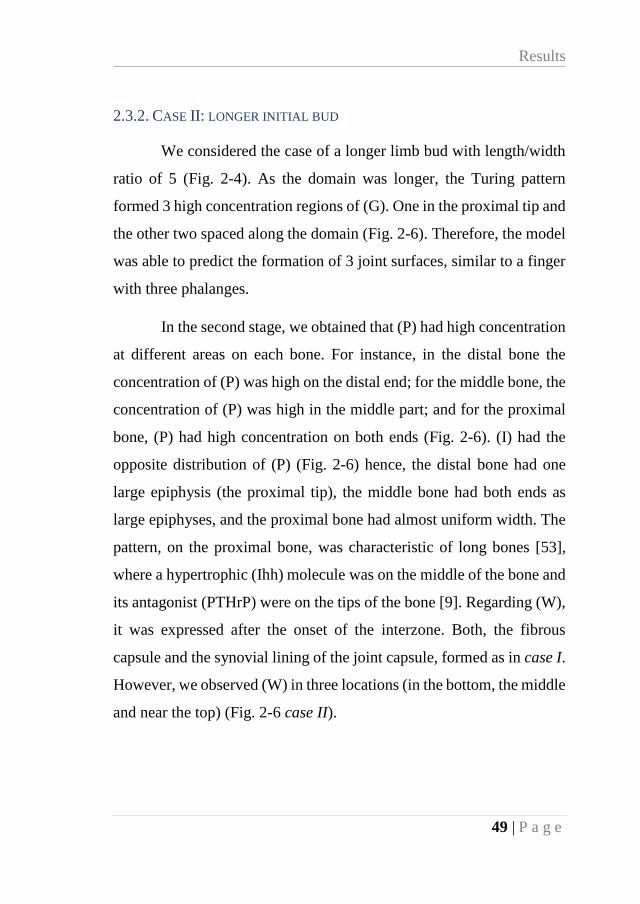
Results
49 | P a g e
2.3.2. CASE II: LONGER INITIAL BUD
We considered the case of a longer limb bud with length/width
ratio of 5 (Fig. 2-4). As the domain was longer, the Turing pattern
formed 3 high concentration regions of (G). One in the proximal tip and
the other two spaced along the domain (Fig. 2-6). Therefore, the model
was able to predict the formation of 3 joint surfaces, similar to a finger
with three phalanges.
In the second stage, we obtained that (P) had high concentration
at different areas on each bone. For instance, in the distal bone the
concentration of (P) was high on the distal end; for the middle bone, the
concentration of (P) was high in the middle part; and for the proximal
bone, (P) had high concentration on both ends (Fig. 2-6). (I) had the
opposite distribution of (P) (Fig. 2-6) hence, the distal bone had one
large epiphysis (the proximal tip), the middle bone had both ends as
large epiphyses, and the proximal bone had almost uniform width. The
pattern, on the proximal bone, was characteristic of long bones [53],
where a hypertrophic (Ihh) molecule was on the middle of the bone and
its antagonist (PTHrP) were on the tips of the bone [9]. Regarding (W),
it was expressed after the onset of the interzone. Both, the fibrous
capsule and the synovial lining of the joint capsule, formed as in case I.
However, we observed (W) in three locations (in the bottom, the middle
and near the top) (Fig. 2-6 case II).
Joint Onset
50 | P a g e
2.3.3. CASE III: HIGH GROWTH RATE
In Case III, the growth rates (expressed as 𝛼𝑖 , 𝛽𝑖, 𝜇𝑖) were
greater than in other cases. As a result, an accelerated growth of the
segments was produced. As in Case I, a single joint was predicted.
However, since the growth velocity was greater, the final rudiments
were much larger compared to the case I (Fig. 2-5 and Fig. 2-6).
Additionally, the distributions of (P) and (I) that were obtained were
different than case I; in this case, molecule (I) had high concentrations
on both ends of the rudiments, whereas for Case I only on one end of
the rudiments. This indicates that growth rate may determine whether
the rudiment will have an epiphysis on one end or at both ends.
2.3.4. CASE IV: WIDER RUDIMENT
For this case, we considered a length/width ratio of 2.5 and
obtained a joint between a large bone and a shorter one. Furthermore,
two joint regions were obtained, one in the proximal end and a second
one close to the distal end (Fig. 2-6). The distal bone had a high
concentration of (I) at the proximal end. As a result, the cells on this
zone would hypertrophy and the proximal head of the distal bone would
have volumetric expansion, similar to Case I. Even though, the
proximal bone was larger, its molecular patterns of (P) and (I) are
similar to those seen clinically on a long bone [53], where PTHrP had
a high concentration in the ends of the bone and Ihh was high close to
the mineralization zone (in the hypertrophic zone of the growth plate).
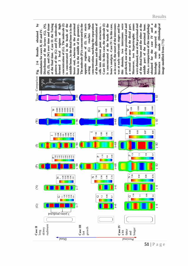
Results
51 | P a g e
Fig
. 2
-6
Resu
lts
ob
tain
ed
b
y
sim
ula
tio
n f
or c
ase
s II
, II
I a
nd
IV
.
Dis
trib
uti
on
o
f th
e
facto
rs
(G),
(N
),
(P),
(I)
, a
nd
(W
) o
ver t
ime
an
d t
issu
e
at
the f
ina
l ti
me.
-Ca
se I
I: t
he T
uri
ng
pa
ttern
of
the (
G)
an
d (
N)
mole
cu
les
form
ed
3
loca
l re
gio
ns
of
hig
h
co
nce
ntr
ati
on
of
(G).
Th
e m
ole
cu
le (
I)
is
co
ncen
tra
ted
in
th
e
hea
ds
of
the
mid
dle
bo
ne, in
th
e d
ista
l b
on
e is
in t
he
low
er en
d,
wh
erea
s in
th
e p
roxim
al
bo
ne
is i
n t
he m
idd
le o
f it
s geom
etr
y.
Th
e m
ole
cu
le (
P)
is c
on
cen
tra
ted
in
th
e
op
po
site
reg
ion
s o
f (I
).
(W)
starts
acti
ng
a
fter
(G
) rea
ch
es
hig
h
co
nce
ntr
ati
on
, m
ark
ing
th
e s
ep
ara
tio
n
of
the b
on
es
an
d t
he d
iffe
ren
tia
tio
n o
f
cell
s in
to d
iffe
ren
t jo
int
stru
ctu
res.
-
Ca
se I
II:
In t
his
ca
se,
the
mo
lecu
le (
I)
is
co
ncen
tra
ted
a
t th
e
hea
ds
of
the
bo
ne’s
an
alg
en
. -C
ase
IV
: In
th
is c
ase
,
as
in c
ase
II,
th
e o
nse
t o
f th
e in
terzo
nes
wa
s a
t early
em
bryo
nic
sta
ges
an
d f
or
this
d
om
ain
, tw
o
inte
rzo
nes
were
pred
icte
d, o
ne a
t th
e p
roxim
al en
d a
nd
a s
eco
nd
on
e n
ear
to t
he
dis
tal
part.
Mo
reov
er,
two
h
yp
ertr
op
hic
zo
nes
were
ob
tain
ed
, on
e a
t th
e p
rox
imal en
d
of
the
dis
tal
bo
ne a
nd
th
e o
ther
at
the
mid
dle
p
art
of
the
pro
xim
al
bon
e.
Als
o, a
co
mp
aris
on
of
the
mo
rp
ho
log
y
ob
tain
ed
fo
r
the
ca
se
IV
an
d
a
his
tolo
gic
st
ud
y
rep
orte
d
in
the
lite
ra
ture
w
as
ma
de
(His
tolo
gic
al
ima
ge m
od
ifie
d f
rom
[7
9])
.
Joint Onset
52 | P a g e
2.3.5. CASE V: IMPLANTATION OF BEADS BEARING GDF-5 (LATERAL)
For this case, we considered that the length/width ratio was 3,
as in Case I. A bead of GDF-5 (Concentration 𝑆𝐺 = 1.5) was placed in
the distal and lateral part of the rudiment to simulate the experimental
scenario according to [77], where a GDF-5 bead was placed on the side
of a developing chick autopod.
On this model, the (I) molecule started to accumulate near the
zone of the bead of GDF-5 and then it formed an intercalated stripe-like
pattern. (P) was inhibited when there is a high concentration of (I); the
latter promoted cell hypertrophy, making the tissue to grow at a greater
rate than the surrounding area (Fig. 2-7). Moreover, the diffusion of the
(W) molecule was expressed in the zone where the (G) molecule was
seeded. Therefore, the shape of the future bone was affected, due to the
modified molecular pattern which altered bone growth. Also, no joint
was formed inside the domain as consequence of the abnormal growth
and molecular patterns, matching the experimental results.
2.3.6. CASE VI: IMPLANTATION OF BEADS BEARING GDF-5 (TIP)
A seed of high concentration of GDF-5 (concentration, 𝑆𝐺 =
1.5) was planted on the tip of the phalanx as it was previously reported
[77]. Since there was a high concentration of (G) on the tip of the
rudiment, the (G-N) patterns were disturbed and no interzone was
formed, therefore there was an absence of joint.
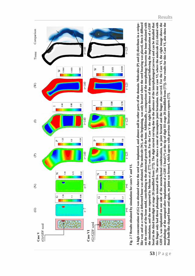
Results
53 | P a g e
Fig
. 2
-7 R
esu
lts
ob
tain
ed
by
sim
ula
tio
n f
or
case
s V
an
d V
I.
A h
igh
co
ncen
tra
tio
n o
f (G
) w
as
ob
tain
ed
wh
ere
the
seed
wa
s im
pla
nte
d, a
nd
alm
ost
nu
ll i
n o
ther
parts
of
the d
om
ain
. M
ole
cu
les
(P)
an
d (
I) d
istr
ibu
te i
n a
str
ipe-
lik
e w
ay
an
d a
s a
resu
lt a
defo
rmed
bo
ne
wa
s o
bta
ined
. T
he m
ole
cu
le (
W),
at
the b
egin
nin
g,
wa
s o
nly
lo
cate
d w
here
th
e se
ed
bea
rin
g w
as
pla
ced
, th
en
it
dif
fuse
d
on
th
e c
on
tou
r o
f th
e b
on
e m
old
, con
trib
uti
ng
to
th
e a
bn
orm
al
gro
wth
of
the b
on
e. A
dd
itio
nall
y, a
co
mp
ari
son
of
the m
orp
holo
gy
betw
een
th
e b
on
e o
bta
ined
wit
h
the s
imu
lati
on
, a
nd
th
e o
ne r
ep
orte
d b
y M
eri
no
et
al.
[7
7]
wa
s m
ad
e.
Fo
r t
he C
ase
V t
he r
igh
t fi
gu
re s
ho
ws
of
the a
uto
po
d f
oll
ow
ing
th
e i
mp
lan
tati
on
of
a G
DF
bea
d i
n t
he t
hir
d i
nte
rd
igit
at
stag
e 2
8 (
mo
dif
ied
fro
m [
77
]).
Th
e d
igit
sta
rte
d c
urvin
g d
ue t
o t
he a
bse
nce
of
the i
nte
rp
hala
ng
eal
(arr
ow
) a
nd
ca
n b
e d
eta
iled
th
at
this
fin
ger
on
ly h
ad
th
ree
ph
ala
ng
es i
nst
ead
of
fiv
e.
Th
e arro
w s
ho
ws
a z
on
e o
f in
com
ple
te j
oin
t fo
rm
ati
on
. O
n o
ur
case
VI,
wh
ere
the
mo
lecu
le (
G)
rel
ate
d w
ith
GD
F-5
, w
as
imp
lan
ted
on
on
e s
ide o
f th
e m
ese
nch
ym
al
co
nd
en
sati
on
, n
o j
oin
t fo
rm
ed
an
d t
he f
ing
er a
lso c
urved
. F
or t
he C
ase
VI,
th
e r
igh
t im
age s
ho
ws
the
morp
holo
gy
of
the a
uto
po
d a
fter i
mp
lan
tati
on
of
a G
DF
-5 b
ead
(*
) a
t th
e t
ip o
f d
igit
III
-sta
ge
28
(m
od
ifie
d f
ro
m [
77
]).
Ou
r r
esu
lts
for t
his
Ca
se V
I, a
lso
sh
ow
th
e
fin
al
bu
lb-l
ike s
ha
ped
bo
ne
an
d a
gain
, n
o j
oin
t w
as
form
ed
, w
hic
h a
gree
s w
ith
prev
iou
s li
tera
ture
rep
orts
[7
7].

Joint Onset
54 | P a g e
The (P) molecule started to accumulate in the center of the bone
anlage and then became more concentrated in the extreme where the
seed was planted. However, its distribution was shapeless (Fig. 2-7). As
in the previous case, there was a high accumulation of (W) where the
(G) seed was planted.
2.4. DISCUSSION
Previous works have shown the molecule interactions for the
digit patterning onset. On the work of Raspopovic et al. [80], they
propose that the digit patterning is controlled by a BMP-Sox9-Wnt
Turing network, which is also controlled by two morphogens (Hox
genes and Fibroblast Growth Factor (FGF) signaling)[80]. Wnt
concentration is high in the interdigital zone, which repress the
chondrogenesis and the expression of Sox9, limited to the digits,
whereas BMP, is out of phase with Sox9, and it is also found on the
digits [80]. Hox gens are in charge of limiting the Turing instability in
the interdigital region, then the digit patterning is independent from the
rest of the skeleton. Finally, FGF, which have not shown a periodic
pattern but only a proximo-distal gradient, being highest in the apical
ectodermal ridge (AER), controls the wavelength and prevent
bifurcations [80].
In this study, we have developed a reaction-diffusion model to
simulate the biochemical system that regulates joint formation, starting
from the last stage analyzed by Raspopovic et al. [80], right after the
digit patenting. We assumed that inside the phalanges anlagen is an
enzyme substrate process between the proteins (N) and (G), a BMP
Discussion
55 | P a g e
molecule which determines where joint cleavage occurs. This first loop
of proteins is essential to the formation of the interzone. (G) demarks
the interzone and (N) establishes a regulatory loop to avoid other zones
from reaching this condition. After cleavage, a negative feedback loop
of proteins (P) and (I) determine where cartilage hypertrophy occurs.
(I) establishes the growth of the articular and hyaline cartilage. In those
areas, where the level of (P) is low, the potential zones for hypertrophy
and mineralization are established. All these four molecules had a
random initial condition. A gradient in molecule (H) was represented
from proximal to distal, during the entire simulation, which was in
charge of increasing domain length. Finally, molecule (W) diffused
from the interzone joint cells to promote the differentiation from
mesenchymal to capsule tissue.
We analyzed six different cases, which showed slight
differences between them, either in geometry or in growth rates. For
Case I we can compare the results obtained for the molecule (G) with
expression of GDF-5 obtained through histological studies, to
demonstrate similar distributions (Fig. 2-8). Additionally, the (I) and
(P) loop resulted in a distribution where (P) is near the distal ends and
(I) is at the proximal ends of the rudiment, as seen histologically for Ihh
and PTHrP (Fig. 2-8).
The (W) molecule established the formation of the articular
cartilage on each joint surface and was consistent with distribution of
Wnt in the literature (Fig. 2-8) [81,82]. When we evaluated morphology
changes in the joint (Fig. 2-5), we observed that the shape of the joint
is comparable with the histologic findings [79]; both sides of the joint
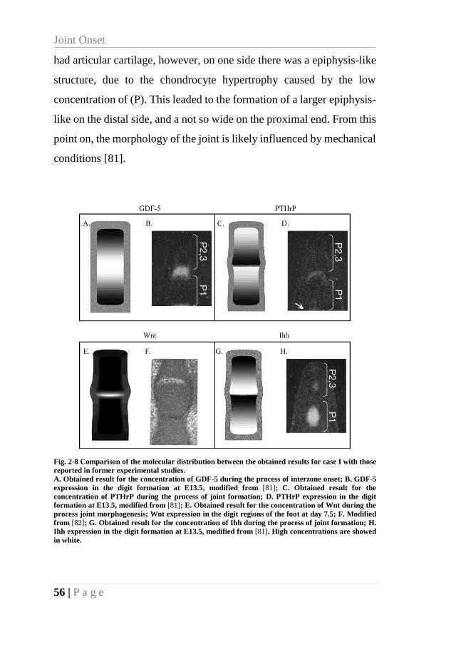
Joint Onset
56 | P a g e
had articular cartilage, however, on one side there was a epiphysis-like
structure, due to the chondrocyte hypertrophy caused by the low
concentration of (P). This leaded to the formation of a larger epiphysis-
like on the distal side, and a not so wide on the proximal end. From this
point on, the morphology of the joint is likely influenced by mechanical
conditions [81].
Fig. 2-8 Comparison of the molecular distribution between the obtained results for case I with those
reported in former experimental studies.
A. Obtained result for the concentration of GDF-5 during the process of interzone onset; B. GDF-5
expression in the digit formation at E13.5, modified from [81]; C. Obtained result for the
concentration of PTHrP during the process of joint formation; D. PTHrP expression in the digit
formation at E13.5, modified from [81]; E. Obtained result for the concentration of Wnt during the
process joint morphogenesis; Wnt expression in the digit regions of the foot at day 7.5; F. Modified
from [82]; G. Obtained result for the concentration of Ihh during the process of joint formation; H.
Ihh expression in the digit formation at E13.5, modified from [81]. High concentrations are showed
in white.
Discussion
57 | P a g e
Our results suggest that the size of the initial domain during
development may have an influence on the number of joints formed.
When the length/width ratio was 3, one joint was obtained, but when
this ratio was increased to 5, three joints were acquired in the
simulation. This result is related to the fact that Turing patterns depend
on the domain ratio, therefore the number of joints will be subject to the
initial ratio. However, literature show that one joint form at a time
[83,84], therefore, it could be possible that each time that the distal
blastema reach a ratio of 3 (approx.), a joint is formed.
At the beginning of the process, growth is not as volumetric
(isotropic) as it is directional (by gradient), with time the growth
becomes mainly volumetric in some zones and in others mostly
directional [46,57]. For instance, for the articular cartilage, growth is
mostly volumetric (due to the concentration of the molecules) and will
define the epiphysis. Whereas for pre-cartilaginous and mesenchymal
tissue, growth is influenced by both, the concentration and the
directional growth.
For a faster growth velocity (case III), we obtain a single joint
with two growing regions, located at both ends of the rudiments (high
concentration of (I) at the ends of the bones). Regarding case IV, we
started with a domain with a length/width ratio of 2.5 and with constant
values specified in Appendix A. In this case, the goal was to simulate
the onset of a joint located between a large bone and a shorter one. This
configuration is similar to a joint between a metatarsal or metacarpal
bone and a phalanx (Fig. 2-6), where we have a large bone on the
proximal side and a shorter one on the distal side. For the proximal
Joint Onset
58 | P a g e
anlage, the molecular distribution (P-I) was similar to that of a large
bone, where the PTHrP molecule is established on the heads of the bone
and Ihh on the middle part [53].
In case V and case VI, we simulated a study performed by
Merino et al., [77]. They analyzed the effects of GDF-5 local
administration in the developing autopod of embryonic chicks. They
implanted GDF-5 beads at the tip of the digits that promoted intense
cartilage growth and failed to induce morphological or molecular signs
of joint formation [77]. Additionally, they implanted GDF-5 beads in
the interdigit joints, which resulted in an inhibition of the formation of
joints in the adjacent digits. This suggests that the role of GDF-5 is to
control growth and differentiate the cartilage of the epiphyseal regions
from the phalanges, rather than accounting for the differentiation of the
synovial joint tissues [77].
When we compare the results obtained in this study for case V
and case VI with those reported in Merino et al. [77] (Fig. 2-7), the
morphology achieved in both studies were similar. We did not obtain
any joint due to the effect of the implantation of the molecule (G), which
modified the Turing patterns, whereas on the Merino et al. [77]
experimentation the GDF-5 beds were added shortly after joints were
formed (Fig. 2-7). Moreover, when we simulated the implantation of
the molecule on one side of the mesenchymal condensation, the
resulting rudiment was curved, as reported in Merino et al., [77] (Fig.
2-7). Similarly, when we simulated the implantation of the molecule
(G) on the tip of the mold, a bulb was formed, as well as in Merino et
al., [77] (Fig. 2-7). These effects could be due to the fact that high
Discussion
59 | P a g e
concentrations of (G) implies, after the cavitation process, high
concentrations of (W), which differentiate the tissue into articular
cartilage. This abnormal location of articular cartilage impacts on the
Turing pattern between (I) and (P), hence abnormal growth of the tissue
is obtained.
In this work, a simplified model to study development of joints
was proposed. This model considered 6 generic factors, which predicted
location of the joint, cavitation, and morphology. There was good
agreement between the obtained results from our simulation model and
those reported in the literature from experimental works, where
histological analyses were performed.
However, during prenatal development, there are additional
factors such as mechanical, genetic, and environmental aspects. We
modeled generic molecules, as there are often multiple molecules that
influence the same biological process. Nonetheless, we showed that
simple pattern formation between enzyme-substrate molecules predicts
many events related to the joint formation. In this model, we used
simplified initial geometry and demonstrated that the initial
length/width relation is crucial to pattern formation. We assumed null
flux at the boundaries of our rudiment, which may not sufficiently
represent communication of the rudiment with surrounding tissues.
However, it was a necessary approximation given the lack of data that
demonstrate flux out of the rudiment. We also assumed random initial
molecular distribution and demonstrated the influence of altering the
initial conditions (with beads of molecule G). The random distribution
is a necessary assumption of the initial state of the limb bud.
Joint Onset
60 | P a g e
In conclusion, this work proposes a simplified computational
model of the regulatory mechanisms that influence the formation of
joints. All the results obtained were compared with those reported on
former studies, which were qualitatively similar. Then, the proposed
computational model may be the first, and a good approximation, of the
phenomenon of joint formation. The model shows a good response with
interphalangeal and metacarpal/metatarsal-phalanx joint development.
This work will be useful for researchers focused on pathologies
associated with embryo and joint development. Furthermore, this model
could provide new insight and guidelines of experimentation, and of
course, new mathematical and computational models as well.
61 | P a g e
Chapter 3. JOINT MORPHOGENESIS
3.1. INTRODUCTION
As it was said on the previous chapter, joint development is
characterized by 3 steps: interzone onset, cavitation, and
morphogenesis. The interzone determines the joint place within the
bone blastema and it is characterized by cells that stopped their
differentiation to chondrocytes [34,85]. The interzone gives place to the
cavitation process, which leads to the physical separation of the anlagen
[34]. Afterwards, comes the last step of the joint development, its
morphogenesis, within this process the joint molds to its final shape
finishing the joint development process, although some studies have
shown that the morphogenesis of the joints might initiate before the
cavitation process [21,40,86]. During cavitation and morphogenesis
chondrocytes proliferate within the bone rudiments allowing their
growth and shaping [39].
The consequences of an abnormal joint morphogenesis can be
debilitating and jeopardize the life quality of the individual, as for the
case of the developmental dysplasia of the hip (DDH), which has a
frequency of 5 out of 1000 hips [21,87], or in arthrogryposis multiplex
congenita (AMC), which due to an abnormal fibrosis of the muscles the
individual develops multiple joint contractures [88]. Although it is an
important health issue to address, there are still imprecisions
Joint Morphogenesis
62 | P a g e
understanding on how and which factors guide the morphogenesis
process [44].
In fact, experimental and computational studies have shown that
there is a relationship between mechanical stress and the skeletal
morphogenesis, growth, regeneration, maintenance and degeneration
[89–97]. Moreover, in the past, it was assumed that the fetal movement
is one of the factors that affects the joint morphogenesis [21].
Researchers have found malformations at the knee joint when chicks
embryos have been immobilize through neuromuscular blocking agents
[98,99]. Also, it was found that other joints develop fused or with non-
interlocking joint shapes [100]. This aspect has also been explored in
mice genetically modified to have “muscle-less limb”, in which the
joints also developed with malformations, in particular the elbow and
shoulder [101,102]. From those studies, there is no doubt that motion
and loading could affect the morphogenesis process during joint
development. However, there are very few studies that have deeply
explored this issue.
From a computational perspective, two models have been
developed to evaluate the relationship between joint morphogenesis and
mechanical stresses [20,21]. Heegaard et al. (1999) developed an
idealized proximal interphalangeal model, including the mechanical
load provided by the muscles through the tendons, to evaluate the
epiphyseal growth through a modified version of Carter’s ossification
theory [103]. In that study, Heegaard et al. evaluated how the joint
morphogenesis is influenced by the contraction of the muscles,
resulting in a congruent development of the joint’s surfaces. That model
Introduction
63 | P a g e
was the first mechanobiological model that simulated the joint
mechanical environment in the prenatal phase.
On the other hand, experimental studies have found that static
compressive and cyclic compression loads inhibits and promote
cartilage growth, respectively [21,104,105] [106–108]. Using that
experimental results, Giorgi et al. [21] developed a 3D computational
model of the joint morphogenesis, including the joint capsule. They also
analyzed the effect of movement range with different initial shapes of
the joint. In addition, they employed idealized shapes for generic joints
such as ball and socket and hinge and applied typical movements for
each type of joint.
Both aforementioned computational works, the one developed
by Heegaard et al. and the one done by Giorgi et al., used the
hydrostatic stress distribution for describing the growth and joint
morphogenesis [20,21]. Although, those seminal works obtained
important results about the morphogenesis process, the final shapes of
the two opposite rudiments do not match entirely to a real
interphalangeal joint shape; strengthening the fact that biochemical
interactions during bone morphogenesis might be necessary to achieve
congruent joint shapes.
From the biochemical perspective, some experimental works
have identified the biochemical factors that might influence the entire
process of joint development. These works have found that Hox genes,
Bone Morphogenetic Proteins (BMPs), Growth and Differentiation
Factors (GDFs), Wnt, chordin and noggin all influence the interzone
onset and the cavitation process [85,95,109]. Based on these literatures,
Joint Morphogenesis
64 | P a g e
we designed a computational model with the aim of explaining the
interaction of these molecules during the joint onset, as described in the
previous chapter (Joint Onset). The previous chapter explained how
self-regulatory loops of biochemical factors may influence the
interzone onset, cell differentiation, tissue growth, cavitation process
and synovial capsule development. In the previous chapter we
explained how biochemical factors influence the joint development,
from the interzone onset to the cavitation process, in which the joint
took its initial shape due to cell proliferation, however, we did not
model how the joint achieves its definitive shape, the final
morphogenesis.
As it was described, the morphogenesis is regulated by
biochemical and mechanical stimuli. Nevertheless, to date, there is no
experimental or computational model able to accurately explain how a
synovial joint is shaped. Moreover, none of the existing computational
models have integrated the biochemical stimulus as a factor for joint
shaping. Understanding how these biochemical and mechanical stimuli
influence the joint morphogenesis process might be useful for the
prevention and treatment of developmental diseases.
Here, a 2D finite element model of the interphalangeal joint was
developed, which included the synovial capsule as domain surrounding
the bone rudiments. This model considers the biochemical and
mechanical effects on the joint morphogenesis, from the cavitation
stage to the appearance of primary and secondary ossification centers
(POC and SOC). Furthermore, the model was tested to replicate
different conditions that might be present in a pathological context, as
Materials and methods
65 | P a g e
when there is a muscular abnormality or joint malalignment. This
model provides a steppingstone to establish an understanding on the
mechanisms that influence the joint morphogenesis. This study could
be useful for physicians and researchers interested in the design of new
joint’s treatments and skeletal development.
3.2. MATERIALS AND METHODS
In this work a finite element model of a synovial joint
morphogenesis was developed. The model includes the effect of
possible molecules and mechanical factors involved in the joint
morphogenesis process. The model initiates with an approximate
geometry of a synovial joint, interphalangeal joint, after the cavitation.
The initial reference geometry was adapted from the result of a previous
work of the authors [96]. The computational process is as follows: The
distal bone anlage was rotated to simulate the movement of the finger,
only four steps of the movement were evaluated: when the distal
phalanx was at 0º, 30º, 60º and 90º. Stresses were computed elementally
on each position and then were translated into a reference state (at 0º)
and averaged at each element. Once all data was translated to the
reference state, cartilage growth and ossification parameters were
computed. Then, the geometry of the reference state was updated
considering by the stresses and biochemical factors. Thus, this process
continued until the shape of the joint agrees with the shape of an
interphalangeal joint.

Joint Morphogenesis
66 | P a g e
3.2.1. GEOMETRY AND BOUNDARY CONDITIONS
For this model, it was assumed that the finger, viewed on a
sagittal plane, had a cyclic extension-flexion movement, where the
distal phalanx rotated around the proximal phalanx. Four steps of the
movement were evaluated: when the distal phalanx was at 90º, 60º, 30º
and 0º with respect to the vertical line y (Fig. 3-1). The geometry of the
model was approximated and adapted from the last step of the previous
chapter’s result (see Joint Onset).
The domain was meshed employing linear quadrilateral
elements, the size of which was refined until further refinement no
longer yielded noticeable improvements. All the equations were solved
with FEM and implemented in a user element Subroutine in FORTRAN
and solved with ABAQUS v6.13 (Dassault Systèmes).
Fig. 3-1 Schematic representation of the boundary conditions implemented on the model.
The inferior boundary of the proximal phalanx has the central node fixed; the other nodes of the
boundary are allowed to move laterally. Palmar side to the left and dorsal to the right.
Materials and methods
67 | P a g e
3.2.2. MECHANICAL ASPECTS
Regarding the mechanical part of the model, a displacement of
1𝜇𝑚 was to the top surface of the distal rudiment towards the proximal
element at each motion stage (Fig. 3-1) [20]. The displacement had
distal to proximal direction related to the distal phalanx (Fig. 3-1). The
proximal phalanx was fixed on its bottom central node, the other bottom
nodes could move on the lateral direction. For simplicity's sake, some
considerations were made, i.e., the modelling of contact between the
phalanges was avoided by including the synovial capsule, as a
circumference surrounding the joint, with a maximal diameter of 6 mm
and large enough to contain the joint throughout movement sequences
(Fig. 3-2), previous studies have proven that the inclusion of the
synovial capsule does not affect the results of the simulation [21],
instead, it saves computational time.
The bones were initially considered as fully cartilaginous, as
they are at this stage of human development. Additionally, all tissues
were modelled as linear-elastic, isotropic and homogeneous materials;
the cartilage of the anlagen bones was assumed as nearly
incompressible (Poisson’s ratio of 0.49). Each cartilage rudiment
section had a Young’s modulus of 1000 kPa, while the synovial capsule
had a Young’s modulus of 1 kPa; establishing a relation 1000:1 between
the cartilage and the capsule tissues. These material properties were
assumed by the authors as they act as symbolic and are easy scalable to
recreate any other real or unreal conditions. In each iteration, it was
computed stresses (octahedral, hydrostatic and shear) and strains. The
model was developed with a plane strain approach.

Joint Morphogenesis
68 | P a g e
Fig. 3-2 Geometry of the bone anlagen and the synovial capsule.
3.2.3.MOLECULAR ASPECTS
There are many molecules that have a role during joint
development which might influence bone growth, ossification and
shaping. For instance, VEGF is involved in bone angiogenesis, and in
various aspects of bone development, including chondrocyte osteoblast
differentiation, and osteoclast recruitment [110]. Moreover, several
studies have suggested a potential role of TGFα in early bone
development, growth and ossification [111]. During embryonic stages,
TGFα regulates the endochondral ossification, the osteoclast
recruitment, and the vascularization at the primary and secondary
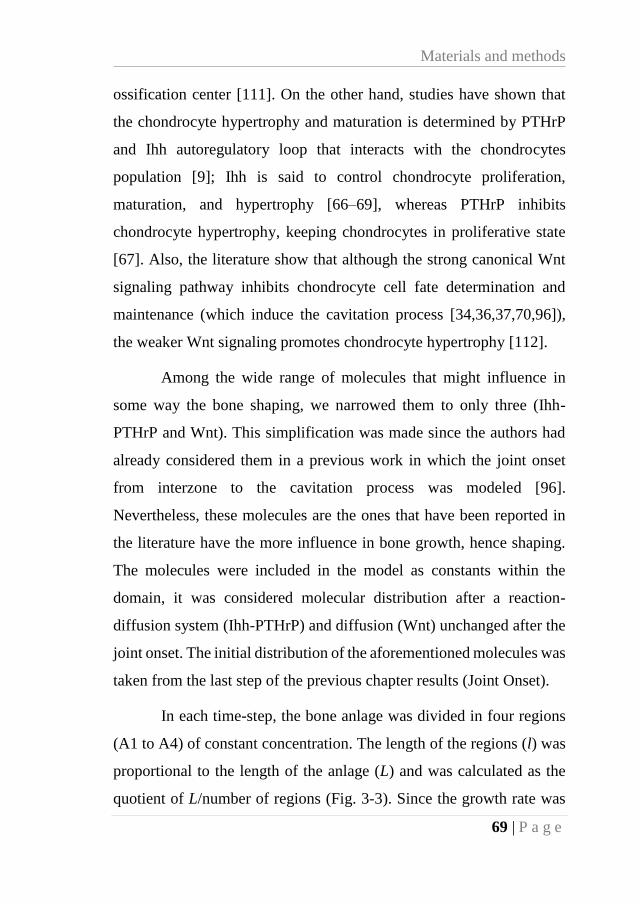
Materials and methods
69 | P a g e
ossification center [111]. On the other hand, studies have shown that
the chondrocyte hypertrophy and maturation is determined by PTHrP
and Ihh autoregulatory loop that interacts with the chondrocytes
population [9]; Ihh is said to control chondrocyte proliferation,
maturation, and hypertrophy [66–69], whereas PTHrP inhibits
chondrocyte hypertrophy, keeping chondrocytes in proliferative state
[67]. Also, the literature show that although the strong canonical Wnt
signaling pathway inhibits chondrocyte cell fate determination and
maintenance (which induce the cavitation process [34,36,37,70,96]),
the weaker Wnt signaling promotes chondrocyte hypertrophy [112].
Among the wide range of molecules that might influence in
some way the bone shaping, we narrowed them to only three (Ihh-
PTHrP and Wnt). This simplification was made since the authors had
already considered them in a previous work in which the joint onset
from interzone to the cavitation process was modeled [96].
Nevertheless, these molecules are the ones that have been reported in
the literature have the more influence in bone growth, hence shaping.
The molecules were included in the model as constants within the
domain, it was considered molecular distribution after a reaction-
diffusion system (Ihh-PTHrP) and diffusion (Wnt) unchanged after the
joint onset. The initial distribution of the aforementioned molecules was
taken from the last step of the previous chapter results (Joint Onset).
In each time-step, the bone anlage was divided in four regions
(A1 to A4) of constant concentration. The length of the regions (l) was
proportional to the length of the anlage (L) and was calculated as the
quotient of L/number of regions (Fig. 3-3). Since the growth rate was
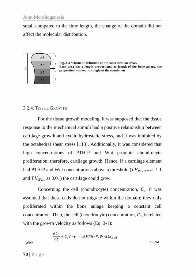
Joint Morphogenesis
70 | P a g e
small compared to the time length, the change of the domain did not
affect the molecular distribution.
Fig. 3-3 Schematic definition of the concentration areas.
Each area has a length proportional to length of the bone anlage, the
proportion was kept throughout the simulation.
3.2.4. TISSUE GROWTH
For the tissue growth modeling, it was supposed that the tissue
response to the mechanical stimuli had a positive relationship between
cartilage growth and cyclic hydrostatic stress, and it was inhibited by
the octahedral shear stress [113]. Additionally, it was considered that
high concentrations of PTHrP and Wnt promote chondrocyte
proliferation, therefore, cartilage growth. Hence, if a cartilage element
had PTHrP and Wnt concentrations above a threshold (𝑇𝐻𝑃𝑇𝐻𝑟𝑃 as 1.1
and 𝑇𝐻𝑊𝑛𝑡 as 0.01) the cartilage could grow.
Concerning the cell (chondrocyte) concentration, 𝐶𝑐, it was
assumed that these cells do not migrate within the domain; they only
proliferated within the bone anlage keeping a constant cell
concentration. Then, the cell (chondrocyte) concentration, 𝐶𝑐, is related
with the growth velocity as follows (Eq. 3-1):
𝑑𝐶𝐶𝑑𝑡
+ 𝐶𝑐∇ ∙ 𝒗 = 𝛼(𝑃𝑇𝐻𝑟𝑃,𝑊𝑛𝑡)𝑆𝐻𝑦𝑑
With Eq. 3-1
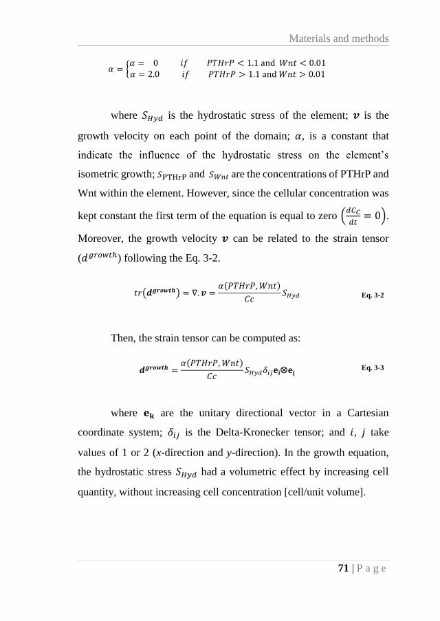
Materials and methods
71 | P a g e
𝛼 = {𝛼 = 0 𝑖𝑓 𝑃𝑇𝐻𝑟𝑃 < 1.1 and 𝑊𝑛𝑡 < 0.01𝛼 = 2.0 𝑖𝑓 𝑃𝑇𝐻𝑟𝑃 > 1.1 and 𝑊𝑛𝑡 > 0.01
where 𝑆𝐻𝑦𝑑 is the hydrostatic stress of the element; 𝒗 is the
growth velocity on each point of the domain; 𝛼, is a constant that
indicate the influence of the hydrostatic stress on the element’s
isometric growth; 𝑆PTHrP and 𝑆𝑊𝑛𝑡 are the concentrations of PTHrP and
Wnt within the element. However, since the cellular concentration was
kept constant the first term of the equation is equal to zero (𝑑𝐶𝐶
𝑑𝑡= 0).
Moreover, the growth velocity 𝒗 can be related to the strain tensor
(𝑑𝑔𝑟𝑜𝑤𝑡ℎ) following the Eq. 3-2.
𝑡𝑟(𝒅𝒈𝒓𝒐𝒘𝒕𝒉) = ∇. 𝒗 =𝛼(𝑃𝑇𝐻𝑟𝑃,𝑊𝑛𝑡)
𝐶𝑐𝑆𝐻𝑦𝑑 Eq. 3-2
Then, the strain tensor can be computed as:
𝒅𝒈𝒓𝒐𝒘𝒕𝒉 =𝛼(𝑃𝑇𝐻𝑟𝑃,𝑊𝑛𝑡)
𝐶𝑐𝑆𝐻𝑦𝑑𝛿𝑖𝑗𝐞𝐢𝐞𝐣
Eq. 3-3
where 𝐞𝐤 are the unitary directional vector in a Cartesian
coordinate system; 𝛿𝑖𝑗 is the Delta-Kronecker tensor; and 𝑖, 𝑗 take
values of 1 or 2 (x-direction and y-direction). In the growth equation,
the hydrostatic stress 𝑆𝐻𝑦𝑑 had a volumetric effect by increasing cell
quantity, without increasing cell concentration [cell/unit volume].

Joint Morphogenesis
72 | P a g e
3.2.5. BONE OSSIFICATION
For the bone ossification it was considered the osteogenic index
(OI). OI was calculated and used to predict the appearance of the POC
and SOC within the anlagen [114–116]. The OI is a scalar parameter
which considers the effect of the hydrostatic stress and the octahedral
shear stress [8]. This parameter, OI, can be used to predict which
regions of the cartilaginous anlage are likely to ossify first (high OI)
[93]. Therefore, the cartilage on the diaphysis was considered to ossify
under high OI (Eq. 3-4) and low PTHrP and Wnt, whereas for the SOC,
only the OI was considered.
𝑂𝐼 = 𝑘1𝑆𝐻𝑦𝑑 + 𝑘2𝑆𝑂𝑐𝑡 Eq. 3-4
𝑆𝐻𝑦𝑑 is the hydrostatic stress; 𝑆𝑂𝑐𝑡 is the octahedral shear stress;
𝑘1 and 𝑘2 are the constants weighting the contribution of 𝑆𝐻𝑦𝑑 and 𝑆𝑂𝑐𝑡,
respectively. 𝑘1 took the value of 0.7 and 𝑘2 of 1 for the proximal
phalanx, and for the distal of -0.35 and 1 for 𝑘1 and 𝑘2, respectively.
The ossification process of the tissue, POC and SOC, was assumed as
a mineralization of the tissue which increased the Young’s modulus of
the element until it reached 20000 kPa.
3.2.6. TRANSLATION TO REFERENCE
At each time-step, a static implicit FEM analysis was done at
each flexion position (90º, 60º, 30º and 0º), then, the results were
translated to a reference position (which is at 0º). Once all the results
were at the reference position, they could be averaged in a unique

Materials and methods
73 | P a g e
geometry where the cartilage growth and ossification were calculated.
This was done by calculating the centroid of each element of the rotated
state (red) and pivot them to the coordinates on the reference state (0º)
(blue), these centroids carry the information about the stresses of the
each element (Fig. 3-4). Afterwards, each element of the reference state
(blue) assumes the value of the closest centroid of the rotated state. With
the obtained quantities at reference state, the calculations of OI and
cartilage growth were done, and the geometry of the reference state was
updated. Then, the distal phalanx of this new reference state was rotate
at each analyzed position and process begins again.
Fig. 3-4 Translation process from a rotated state to the reference state at (0º).
Palmar side to the left and dorsal to the right.
3.2.7. GENERAL ALGORITHM
The algorithm proposed for the morphogenesis model is shown
in Fig. 3-5. The computational model initiated with the drawing and
meshing of the geometry at it position (90º, 60º, 30º and 0º), then, the
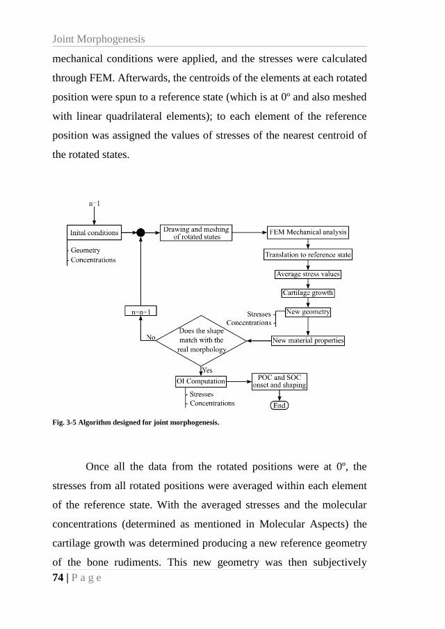
Joint Morphogenesis
74 | P a g e
mechanical conditions were applied, and the stresses were calculated
through FEM. Afterwards, the centroids of the elements at each rotated
position were spun to a reference state (which is at 0º and also meshed
with linear quadrilateral elements); to each element of the reference
position was assigned the values of stresses of the nearest centroid of
the rotated states.
Fig. 3-5 Algorithm designed for joint morphogenesis.
Once all the data from the rotated positions were at 0º, the
stresses from all rotated positions were averaged within each element
of the reference state. With the averaged stresses and the molecular
concentrations (determined as mentioned in Molecular Aspects) the
cartilage growth was determined producing a new reference geometry
of the bone rudiments. This new geometry was then subjectively
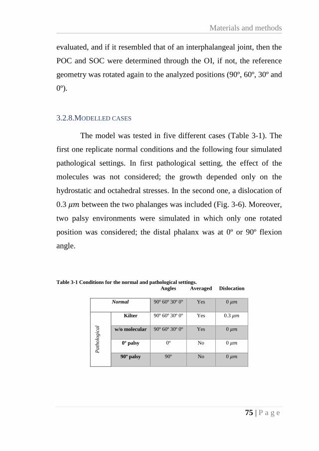
Materials and methods
75 | P a g e
evaluated, and if it resembled that of an interphalangeal joint, then the
POC and SOC were determined through the OI, if not, the reference
geometry was rotated again to the analyzed positions (90º, 60º, 30º and
0º).
3.2.8.MODELLED CASES
The model was tested in five different cases (Table 3-1). The
first one replicate normal conditions and the following four simulated
pathological settings. In first pathological setting, the effect of the
molecules was not considered; the growth depended only on the
hydrostatic and octahedral stresses. In the second one, a dislocation of
0.3 𝜇𝑚 between the two phalanges was included (Fig. 3-6). Moreover,
two palsy environments were simulated in which only one rotated
position was considered; the distal phalanx was at 0º or 90º flexion
angle.
Table 3-1 Conditions for the normal and pathological settings.
Angles Averaged Dislocation
Normal 90º 60º 30º 0º Yes 0 𝜇𝑚
Pa
tho
log
ical
Kilter 90º 60º 30º 0º Yes 0.3 𝜇𝑚
w/o molecular 90º 60º 30º 0º Yes 0 𝜇𝑚
0º palsy 0º No 0 𝜇𝑚
90º palsy 90º No 0 𝜇𝑚
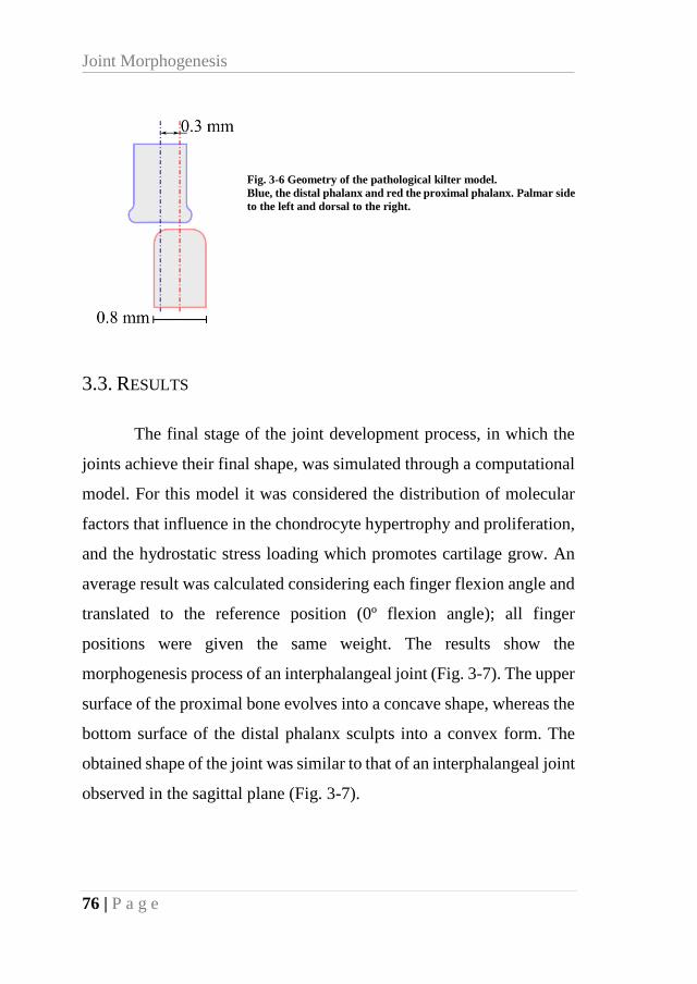
Joint Morphogenesis
76 | P a g e
Fig. 3-6 Geometry of the pathological kilter model.
Blue, the distal phalanx and red the proximal phalanx. Palmar side
to the left and dorsal to the right.
3.3. RESULTS
The final stage of the joint development process, in which the
joints achieve their final shape, was simulated through a computational
model. For this model it was considered the distribution of molecular
factors that influence in the chondrocyte hypertrophy and proliferation,
and the hydrostatic stress loading which promotes cartilage grow. An
average result was calculated considering each finger flexion angle and
translated to the reference position (0º flexion angle); all finger
positions were given the same weight. The results show the
morphogenesis process of an interphalangeal joint (Fig. 3-7). The upper
surface of the proximal bone evolves into a concave shape, whereas the
bottom surface of the distal phalanx sculpts into a convex form. The
obtained shape of the joint was similar to that of an interphalangeal joint
observed in the sagittal plane (Fig. 3-7).
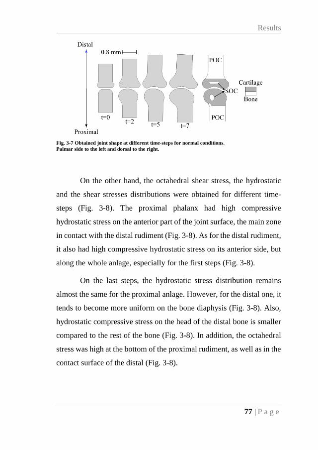
Results
77 | P a g e
Fig. 3-7 Obtained joint shape at different time-steps for normal conditions.
Palmar side to the left and dorsal to the right.
On the other hand, the octahedral shear stress, the hydrostatic
and the shear stresses distributions were obtained for different time-
steps (Fig. 3-8). The proximal phalanx had high compressive
hydrostatic stress on the anterior part of the joint surface, the main zone
in contact with the distal rudiment (Fig. 3-8). As for the distal rudiment,
it also had high compressive hydrostatic stress on its anterior side, but
along the whole anlage, especially for the first steps (Fig. 3-8).
On the last steps, the hydrostatic stress distribution remains
almost the same for the proximal anlage. However, for the distal one, it
tends to become more uniform on the bone diaphysis (Fig. 3-8). Also,
hydrostatic compressive stress on the head of the distal bone is smaller
compared to the rest of the bone (Fig. 3-8). In addition, the octahedral
stress was high at the bottom of the proximal rudiment, as well as in the
contact surface of the distal (Fig. 3-8).
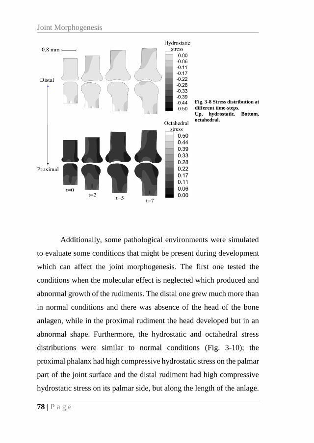
Joint Morphogenesis
78 | P a g e
Fig. 3-8 Stress distribution at
different time-steps.
Up, hydrostatic. Bottom,
octahedral.
Additionally, some pathological environments were simulated
to evaluate some conditions that might be present during development
which can affect the joint morphogenesis. The first one tested the
conditions when the molecular effect is neglected which produced and
abnormal growth of the rudiments. The distal one grew much more than
in normal conditions and there was absence of the head of the bone
anlagen, while in the proximal rudiment the head developed but in an
abnormal shape. Furthermore, the hydrostatic and octahedral stress
distributions were similar to normal conditions (Fig. 3-10); the
proximal phalanx had high compressive hydrostatic stress on the palmar
part of the joint surface and the distal rudiment had high compressive
hydrostatic stress on its palmar side, but along the length of the anlage.
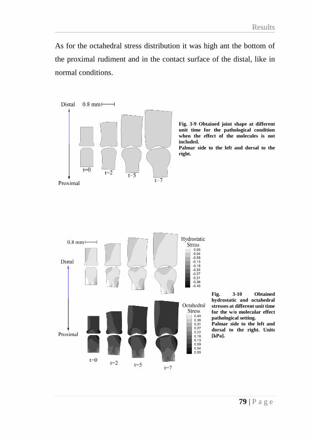
Results
79 | P a g e
As for the octahedral stress distribution it was high ant the bottom of
the proximal rudiment and in the contact surface of the distal, like in
normal conditions.
Fig. 3-9 Obtained joint shape at different
unit time for the pathological condition
when the effect of the molecules is not
included.
Palmar side to the left and dorsal to the
right.
Fig. 3-10 Obtained
hydrostatic and octahedral
stresses at different unit time
for the w/o molecular effect
pathological setting.
Palmar side to the left and
dorsal to the right. Units
[kPa].
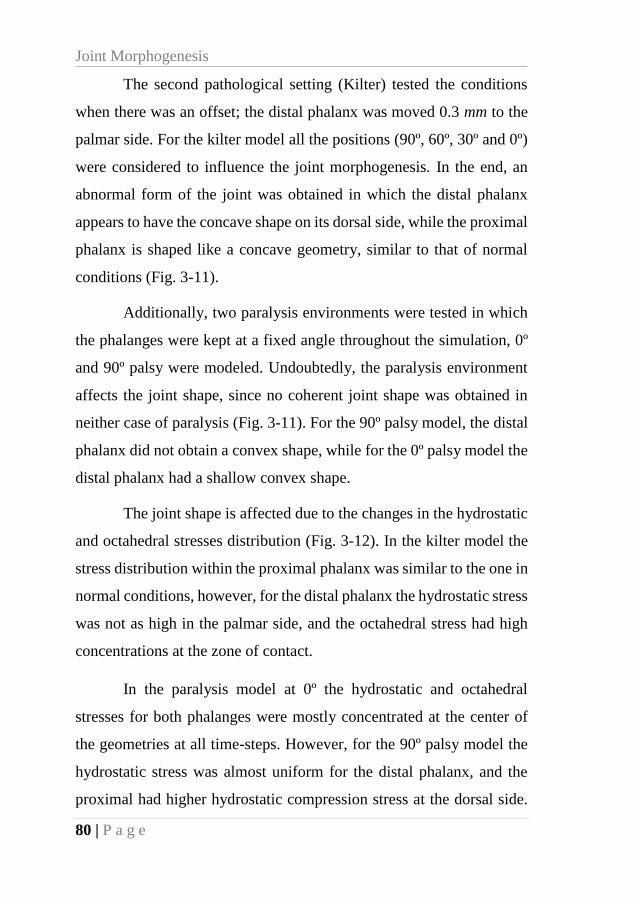
Joint Morphogenesis
80 | P a g e
The second pathological setting (Kilter) tested the conditions
when there was an offset; the distal phalanx was moved 0.3 mm to the
palmar side. For the kilter model all the positions (90º, 60º, 30º and 0º)
were considered to influence the joint morphogenesis. In the end, an
abnormal form of the joint was obtained in which the distal phalanx
appears to have the concave shape on its dorsal side, while the proximal
phalanx is shaped like a concave geometry, similar to that of normal
conditions (Fig. 3-11).
Additionally, two paralysis environments were tested in which
the phalanges were kept at a fixed angle throughout the simulation, 0º
and 90º palsy were modeled. Undoubtedly, the paralysis environment
affects the joint shape, since no coherent joint shape was obtained in
neither case of paralysis (Fig. 3-11). For the 90º palsy model, the distal
phalanx did not obtain a convex shape, while for the 0º palsy model the
distal phalanx had a shallow convex shape.
The joint shape is affected due to the changes in the hydrostatic
and octahedral stresses distribution (Fig. 3-12). In the kilter model the
stress distribution within the proximal phalanx was similar to the one in
normal conditions, however, for the distal phalanx the hydrostatic stress
was not as high in the palmar side, and the octahedral stress had high
concentrations at the zone of contact.
In the paralysis model at 0º the hydrostatic and octahedral
stresses for both phalanges were mostly concentrated at the center of
the geometries at all time-steps. However, for the 90º palsy model the
hydrostatic stress was almost uniform for the distal phalanx, and the
proximal had higher hydrostatic compression stress at the dorsal side.
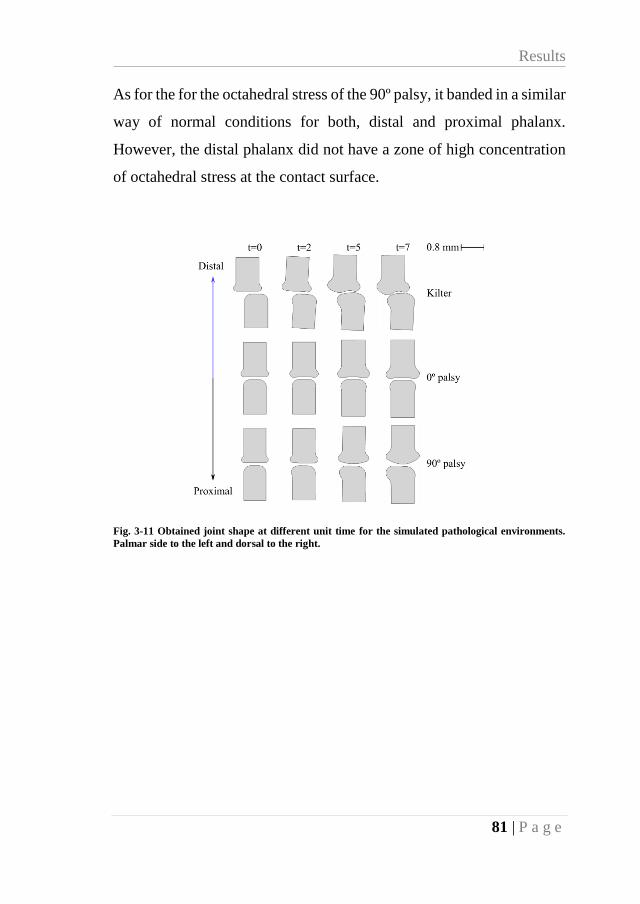
Results
81 | P a g e
As for the for the octahedral stress of the 90º palsy, it banded in a similar
way of normal conditions for both, distal and proximal phalanx.
However, the distal phalanx did not have a zone of high concentration
of octahedral stress at the contact surface.
Fig. 3-11 Obtained joint shape at different unit time for the simulated pathological environments.
Palmar side to the left and dorsal to the right.
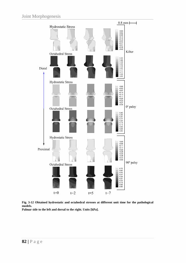
Joint Morphogenesis
82 | P a g e
Fig. 3-12 Obtained hydrostatic and octahedral stresses at different unit time for the pathological
models.
Palmar side to the left and dorsal to the right. Units [kPa].
Discussion
83 | P a g e
3.4. DISCUSSION
Previous works have tried to describe the joint morphogenesis
as a result of cartilage tissue response to hydrostatic stress distribution
[20,21]. They showed how both ends of the bone rudiments changed
their shape according to the hydrostatic stress distribution, however, the
final shapes of the two opposite rudiments do not agree to the
morphology of the joint. Therefore, it confirms that not only the
mechanical environment affects the morphogenesis of the heads of the
bones, but also there are biochemical aspects that should be considered.
From a biochemical point of view, in our previous chapter (Joint
Onset) we analyzed the biochemical interaction of the joint onset, from
the appearance of the interzone to the cavitation process. During these
stages, only the interaction of molecules is responsible to regulate the
joint development. However, during the morphogenesis process it is
also necessary to include the effect of mechanical loading.
In this study, the molecular and mechanical factors, influence
joint morphogenesis. It was assumed that the molecules involved on the
previous steps of joint development, interzone onset and cavitation, also
have influence during the morphogenesis. The distribution of the
molecular factors was kept constant within each time-step of the
domain (Fig. 3-13). The concentration of the molecules in conjunction
with the stresses influenced the growth of the cartilage. As hydrostatic
compression stress, PTHrP and Wnt promote cartilage growth and
chondrocyte proliferation, respectively, in the zones where we have a
high concentration of both, cartilage growth is promoted. For instance,
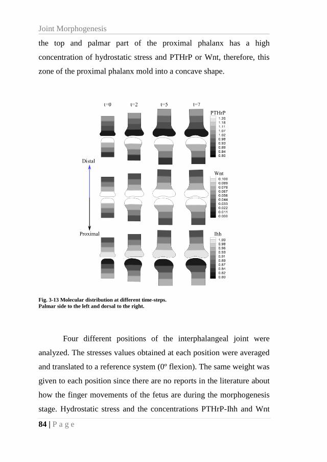
Joint Morphogenesis
84 | P a g e
the top and palmar part of the proximal phalanx has a high
concentration of hydrostatic stress and PTHrP or Wnt, therefore, this
zone of the proximal phalanx mold into a concave shape.
Fig. 3-13 Molecular distribution at different time-steps.
Palmar side to the left and dorsal to the right.
Four different positions of the interphalangeal joint were
analyzed. The stresses values obtained at each position were averaged
and translated to a reference system (0º flexion). The same weight was
given to each position since there are no reports in the literature about
how the finger movements of the fetus are during the morphogenesis
stage. Hydrostatic stress and the concentrations PTHrP-Ihh and Wnt
Discussion
85 | P a g e
were considered to play a role during joint morphogenesis, therefore, in
the zones where we have a high concentration of these molecules and
hydrostatic stress, cartilage growth is promoted. For instance, the top
and anterior part of the proximal phalanx has a high concentration of
hydrostatic stress and PTHrP, therefore, this zone of the proximal
phalanx evolved into a concave shape. Additionally, the distal phalanx
joint surface shaped into a convex structure due to high concentrations
of octahedral shear stress on the center of the joint surface, which
inhibited cartilage growth. The obtained final shapes of the bones’
diaphysis were coherent with those of an interphalangeal joint (Fig.
3-14).
As part of the endochondral ossification, if the effect of the OI
is included, the shapes of SOC and POC can be also explained as seen
in our results (Fig. 3-14). The model showed how the OI predict the
areas of high ossification on the diaphysis. The OI computation was
based on the one proposed by Carter and Wong (1988) [93]. They
established that the OI is calculated based on the octahedral shear stress
and the hydrostatic stress multiplied by an empirical constant 𝑘𝑖. In this
study, the values of the multipliers 𝑘𝑖 were different for each stress and
phalanx, condition which we considered was necessary for a coherent
ossification process. The obtained results are comparable with those
from former studies, where only the endochondral ossification and OI
distribution was analyzed [56,93,116].On the proximal phalanx the
SOC was shaped as a circular structure. On the distal anlage, the SOC
took an elliptical shape, most likely due to how the convex surface
distributed the octahedral shear stress and hydrostatic stresses (OI).
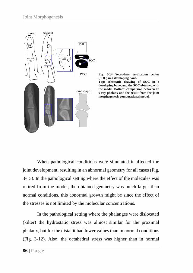
Joint Morphogenesis
86 | P a g e
Fig. 3-14 Secondary ossification center
(SOC) in a developing bone.
Top: schematic drawing of SOC in a
developing bone, and the SOC obtained with
the model. Bottom: comparison between an
x-ray phalanx and the result from the joint
morphogenesis computational model.
When pathological conditions were simulated it affected the
joint development, resulting in an abnormal geometry for all cases (Fig.
3-15). In the pathological setting where the effect of the molecules was
retired from the model, the obtained geometry was much larger than
normal conditions, this abnormal growth might be since the effect of
the stresses is not limited by the molecular concentrations.
In the pathological setting where the phalanges were dislocated
(kilter) the hydrostatic stress was almost similar for the proximal
phalanx, but for the distal it had lower values than in normal conditions
(Fig. 3-12). Also, the octahedral stress was higher than in normal
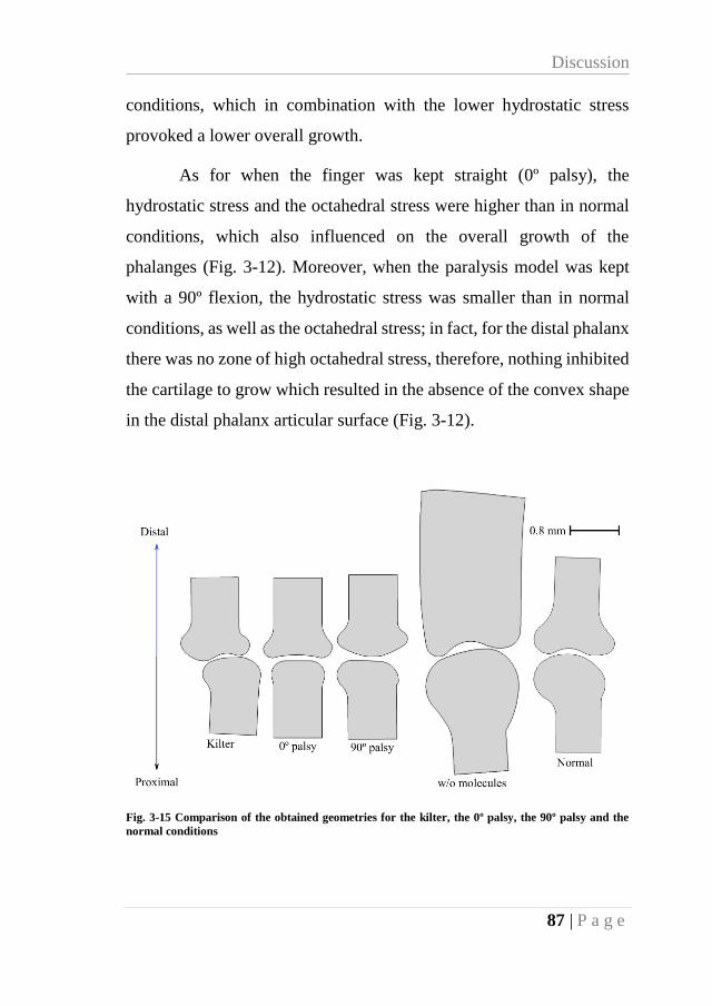
Discussion
87 | P a g e
conditions, which in combination with the lower hydrostatic stress
provoked a lower overall growth.
As for when the finger was kept straight (0º palsy), the
hydrostatic stress and the octahedral stress were higher than in normal
conditions, which also influenced on the overall growth of the
phalanges (Fig. 3-12). Moreover, when the paralysis model was kept
with a 90º flexion, the hydrostatic stress was smaller than in normal
conditions, as well as the octahedral stress; in fact, for the distal phalanx
there was no zone of high octahedral stress, therefore, nothing inhibited
the cartilage to grow which resulted in the absence of the convex shape
in the distal phalanx articular surface (Fig. 3-12).
Fig. 3-15 Comparison of the obtained geometries for the kilter, the 0º palsy, the 90º palsy and the
normal conditions
Joint Morphogenesis
88 | P a g e
The final shape of the normal condition model was compared to
x-ray images of interphalangeal joints (Fig. 3-14). The obtained joint
shape agrees remarkably with the ones observed in the x-rays.
Therefore, this work sheds some light on how the mechanical
environment combined with biochemical factors influence the
morphogenesis of a synovial joint. It is worth mentioning that
hydrostatic stress, as it promotes cartilage growth, is key for joint
morphogenesis. However, for a joint to achieve complex shapes, it is
necessary to include the cell/tissue responses to the biochemical and
mechanical stimuli. The combined response to these stimuli produces
the necessary chondrocyte proliferation and cartilage ECM productions
on specific zones, which molds the bones epiphyses to their final
congruent joint surfaces’ shapes.
To our knowledge, this is the first computational model able to
include several aspects of joint development, such as the main
molecular and mechanical stimuli, and predict, successfully, the final
shape of a synovial joint, like an interphalangeal joint. Moreover, the
model also predicts, thoroughly, the molecular distribution of the
principal biochemical within the developing bone, as well as the onset
of POC and SOC.
The obtained results are remarkable despite the assumptions that
had to be made for simplicity’s sake and computational savings. As
limitations for this model is included the fact that this is only a 2D
model, therefore only one plane of motion was included. Additionally,
some simplifications were made regarding the material behavior and
properties. Likewise, since there is no information related to embryo
Discussion
89 | P a g e
movement during development, and much less in relation to the fetus
finger motion, all the analyzed positions were considered to have the
same weight and influence on the morphogenesis process.
Nevertheless, the presented model gives an excellent approximation of
what is happening during joint development and morphogenesis and
brings a new understanding of these processes, which, eventually, may
lead to the development of new treatments for developmental diseases,
or even prevent malformations of the fetus.


91 | P a g e
Chapter 4. PATELLA ONSET
4.1. INTRODUCTION
Although the development of the skeletal system has been
studied over the past centuries, the development of a group of bones
known as sesamoid bones is still unknown [117]. Sesamoid bones, such
as the patella, are bones embedded superficially within tendons; these
tendons are usually around joints. The name sesamoid comes from the
Latin word sesamum (sesame seed), due to the small size of most of
these bones, and the morphological resemblance of this bone to the seed
[117]. Sesamoid bones can be found in several joints throughout the
body, including hand, wrist, foot, neck, ear and knee. The patella, or
kneecap, is the largest, most recognized and studied sesamoid bone in
the human body.
The patella has an important role in the stability of the knee,
facilitating the function and locomotion of the lower limb [118]. It is
believed that its main purpose is to increase the moment arm of the
quadriceps muscle, by augmenting the distance between this muscle
and the center of rotation of the knee joint [119]. The patella contributes
to the compressive force distribution of the patella-femoral joint by
increasing the contact area during flexion of the knee [119]. In addition,
the patella protects the quadriceps tendon from high stress [120], while
centralizing the pull of the quadriceps muscle complex, protecting the
knee from dislocating [119].
Patella Onset
92 | P a g e
The accepted theory about the development of the patella is that
it develops inside the tendon in response to mechanical stimuli evoked
when the muscles contract [114,117,121]. This theory is based on the
idea that mechanical stimuli play a crucial role in tissue differentiation
[7]. Therefore, while the tendon is immature, a zone of the tendon is
subjected to high hydrostatic stress and low tensile strain. This leads to
the differentiation of the fibrous tissue into cartilage and then to the
ossification of the cartilage to form the patella.
According to the aforementioned tissue adaptation theory,
Topological Optimization (TO) may also be suitable to explain the
development of the patella. TO distributes the material in a design
domain through the minimization of the strain energy; as a result, this
material redistribution produces an optimal configuration for low
energy consumption [122]. This theory has been widely used in many
engineering and biology fields, such as the architecture of the proximal
femur [123–126] as well as in the design of scaffolds, implants, bone
replacements, and prostheses [127–130].
On the other hand, a recent study [117] proposed that the patella
initially develops as part of the femur, similar to the way in which a
bone eminence is developed. This eminence is initially formed by
progenitor cells that express both Sox9 and Scx. This mechanism is
controlled by Transforming Growth Factor-Beta (TGF-β) and Bone
Morphogenetic Protein-4 (BMP-4), which determine the differentiation
of chondrogenic cells. According to this theory, the eminence is
separated from the preexisting cartilaginous femur under different
environmental conditions, but they consider more plausible that the
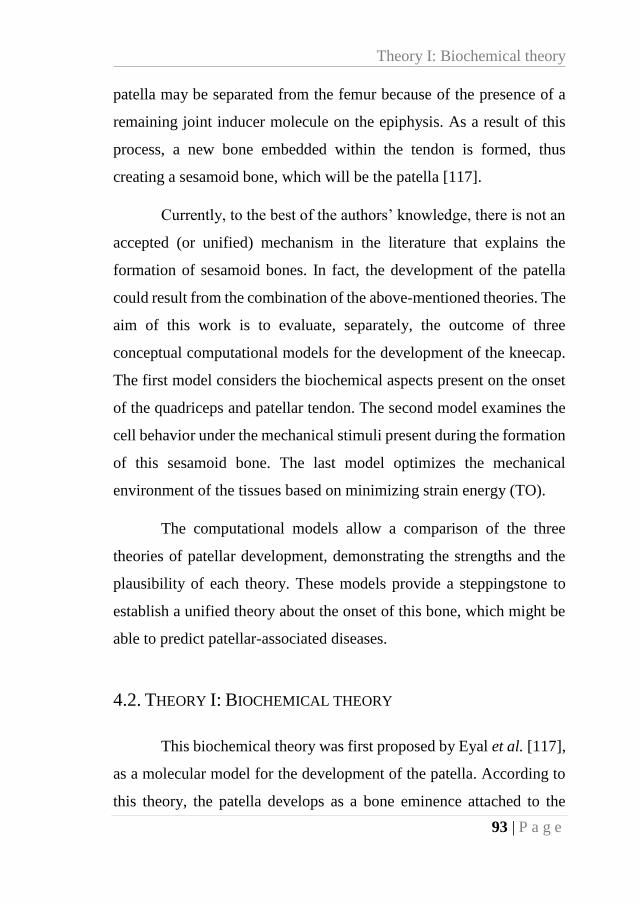
Theory I: Biochemical theory
93 | P a g e
patella may be separated from the femur because of the presence of a
remaining joint inducer molecule on the epiphysis. As a result of this
process, a new bone embedded within the tendon is formed, thus
creating a sesamoid bone, which will be the patella [117].
Currently, to the best of the authors’ knowledge, there is not an
accepted (or unified) mechanism in the literature that explains the
formation of sesamoid bones. In fact, the development of the patella
could result from the combination of the above-mentioned theories. The
aim of this work is to evaluate, separately, the outcome of three
conceptual computational models for the development of the kneecap.
The first model considers the biochemical aspects present on the onset
of the quadriceps and patellar tendon. The second model examines the
cell behavior under the mechanical stimuli present during the formation
of this sesamoid bone. The last model optimizes the mechanical
environment of the tissues based on minimizing strain energy (TO).
The computational models allow a comparison of the three
theories of patellar development, demonstrating the strengths and the
plausibility of each theory. These models provide a steppingstone to
establish a unified theory about the onset of this bone, which might be
able to predict patellar-associated diseases.
4.2. THEORY I: BIOCHEMICAL THEORY
This biochemical theory was first proposed by Eyal et al. [117],
as a molecular model for the development of the patella. According to
this theory, the patella develops as a bone eminence attached to the
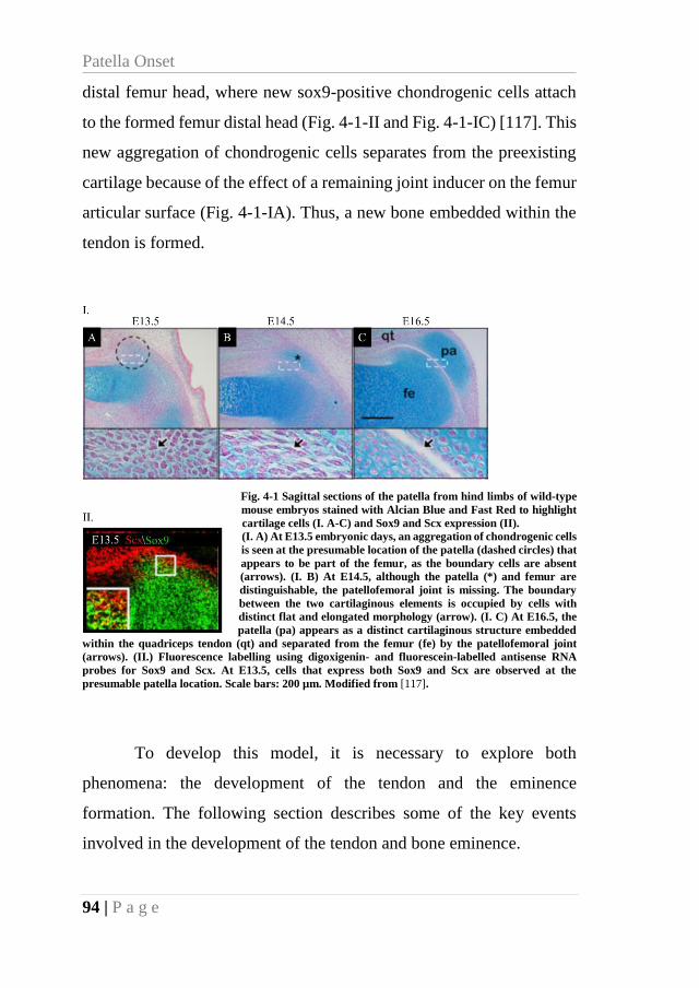
Patella Onset
94 | P a g e
distal femur head, where new sox9-positive chondrogenic cells attach
to the formed femur distal head (Fig. 4-1-II and Fig. 4-1-IC) [117]. This
new aggregation of chondrogenic cells separates from the preexisting
cartilage because of the effect of a remaining joint inducer on the femur
articular surface (Fig. 4-1-IA). Thus, a new bone embedded within the
tendon is formed.
Fig. 4-1 Sagittal sections of the patella from hind limbs of wild-type
mouse embryos stained with Alcian Blue and Fast Red to highlight
cartilage cells (I. A-C) and Sox9 and Scx expression (II).
(I. A) At E13.5 embryonic days, an aggregation of chondrogenic cells
is seen at the presumable location of the patella (dashed circles) that
appears to be part of the femur, as the boundary cells are absent
(arrows). (I. B) At E14.5, although the patella (*) and femur are
distinguishable, the patellofemoral joint is missing. The boundary
between the two cartilaginous elements is occupied by cells with
distinct flat and elongated morphology (arrow). (I. C) At E16.5, the
patella (pa) appears as a distinct cartilaginous structure embedded
within the quadriceps tendon (qt) and separated from the femur (fe) by the patellofemoral joint
(arrows). (II.) Fluorescence labelling using digoxigenin- and fluorescein-labelled antisense RNA
probes for Sox9 and Scx. At E13.5, cells that express both Sox9 and Scx are observed at the
presumable patella location. Scale bars: 200 µm. Modified from [117].
To develop this model, it is necessary to explore both
phenomena: the development of the tendon and the eminence
formation. The following section describes some of the key events
involved in the development of the tendon and bone eminence.
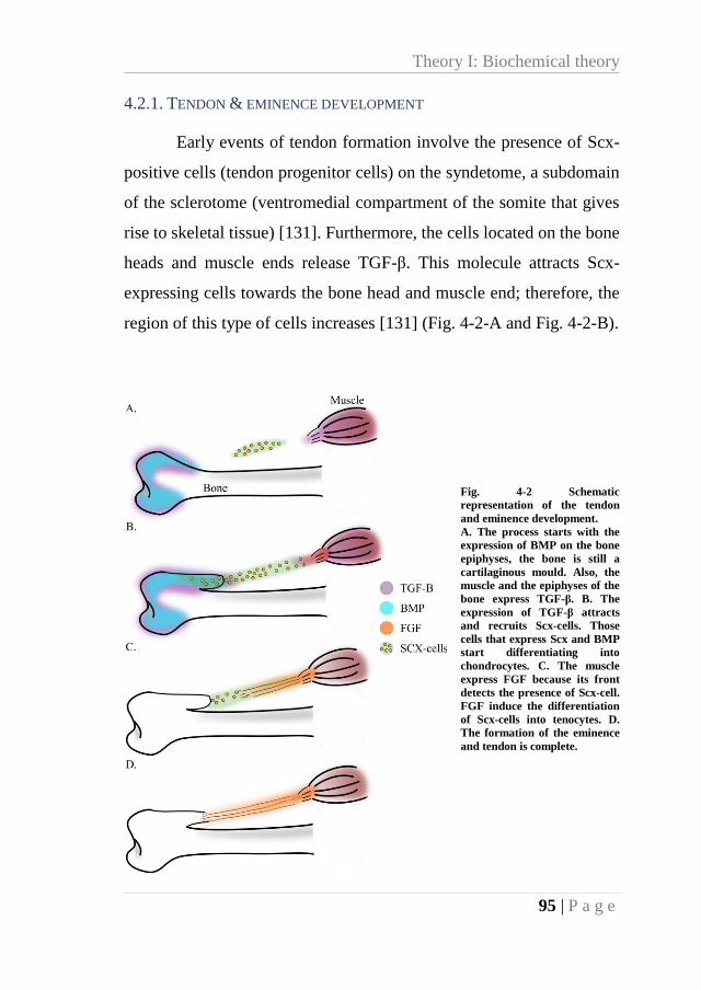
Theory I: Biochemical theory
95 | P a g e
4.2.1. TENDON & EMINENCE DEVELOPMENT
Early events of tendon formation involve the presence of Scx-
positive cells (tendon progenitor cells) on the syndetome, a subdomain
of the sclerotome (ventromedial compartment of the somite that gives
rise to skeletal tissue) [131]. Furthermore, the cells located on the bone
heads and muscle ends release TGF-β. This molecule attracts Scx-
expressing cells towards the bone head and muscle end; therefore, the
region of this type of cells increases [131] (Fig. 4-2-A and Fig. 4-2-B).
Fig. 4-2 Schematic
representation of the tendon
and eminence development.
A. The process starts with the
expression of BMP on the bone
epiphyses, the bone is still a
cartilaginous mould. Also, the
muscle and the epiphyses of the
bone express TGF-β. B. The
expression of TGF-β attracts
and recruits Scx-cells. Those
cells that express Scx and BMP
start differentiating into
chondrocytes. C. The muscle
express FGF because its front
detects the presence of Scx-cell.
FGF induce the differentiation
of Scx-cells into tenocytes. D.
The formation of the eminence
and tendon is complete.
Patella Onset
96 | P a g e
On the muscle end, the muscle cells perceive the presence of
Scx-expressing cells and deliver the FGF [132,133]. FGF (that diffuses
from the muscle through the Scx-cells domain) promotes the
differentiation of Scx-expressing cells into tendon cells (tenocytes).
The direction of the FGF gradient determines the direction of the tendon
fibers [132,133] (Fig. 4-2-C).
Simultaneously from the bone side, BMPs, which regulate the
differentiation of Scx-expressing cells into chondrocytes, diffuse from
the bone head [134]. BMP stimulates the Scx-cells to differentiate into
chondrocytes. These chondrocytes will later shape the bone eminence
where the tendon is attached (Fig. 4-2-B and Fig. 4-2-C) [134]. Thus, a
fully formed tendon is obtained between the bone and the muscle (Fig.
4-2-D).
4.2.2. COMPUTATIONAL AND MATHEMATICAL MODEL
The biochemical model simulates the expression and diffusion
of molecular signals during patellar development as proposed by Eyal
et al. [117]. It is based on the formation of the quadriceps and patellar
tendons (Fig. 4-3) and assumes that some molecules are remnants of the
femur-tibia joint formation process [117], such as GDF-5 (Fig. 4-3-a)
[50–52], which later will induce the joint onset between the patella and
the femur.
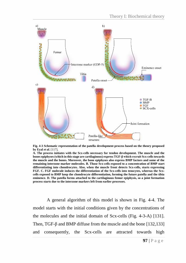
Theory I: Biochemical theory
97 | P a g e
Fig. 4-3 Schematic representation of the patella development process based on the theory proposed
by Eyal et al. [117]. A. The process initiates with the Scx-cells necessary for tendon development. The muscle and the
bones epiphyses (which in this stage are cartilaginous) express TGF-β which recruit Scx-cells towards
the muscle and the bones. Moreover, the bone epiphyses also express BMP factors and some of the
remaining interzone marker molecules. B. Those Scx-cells exposed to a concentration of BMP start
differentiating into chondrocytes. Also, when the muscle front detects Scx-cells, starts expressing
FGF. C. FGF molecule induces the differentiation of the Scx-cells into tenocytes, whereas the Scx-
cells exposed to BMP keep the chondrocyte differentiation, forming the future patella and the tibia
eminence. D. The patella forms attached to the cartilaginous femur epiphysis, so a joint formation
process starts due to the interzone markers left from earlier processes.
A general algorithm of this model is shown in Fig. 4-4. The
model starts with the initial conditions given by the concentrations of
the molecules and the initial domain of Scx-cells (Fig. 4-3-A) [131].
Then, TGF-β and BMP diffuse from the muscle and the bone [132,133]
and consequently, the Scx-cells are attracted towards high
Patella Onset
98 | P a g e
concentration of TGF-β (Fig. 4-3-B). Once the muscle detects the
presence of Scx-cells, it expresses FGF (Fig. 4-3-B) [132,133]. The
differentiation process involves the Scx-cells and the concentrations of
FGF and BMP. If there is enough concentration of Scx-cells and BMP,
the cells in the tissue differentiate into chondrocytes [134], whereas if
there is enough concentration of Scx-cells and FGF, the cells
differentiate into tenocytes (tendon tissue) (Fig. 4-3-B) [132,133]. At
the same time, the remaining interzone marker (in this model named
GDF-5) diffuses inside the newly formed cartilage structure (Fig. 4-3-
C), which will induce later the joint formation between the patella and
the femur (Fig. 4-3-D) [50–52].
Additionally, it is considered that the flexion of the leg during
embryonic stages could influence the patella onset; therefore, this
methodology was applied for different leg angles (30º, 45º, 60º, 90º)
without the modification of any other parameter.
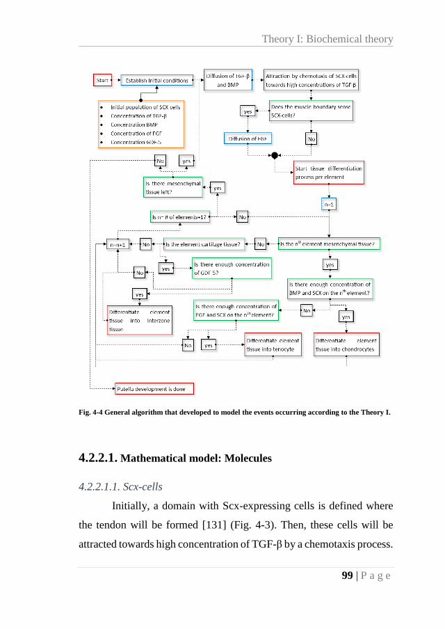
Theory I: Biochemical theory
99 | P a g e
Fig. 4-4 General algorithm that developed to model the events occurring according to the Theory I.
4.2.2.1. Mathematical model: Molecules
4.2.2.1.1. Scx-cells
Initially, a domain with Scx-expressing cells is defined where
the tendon will be formed [131] (Fig. 4-3). Then, these cells will be
attracted towards high concentration of TGF-β by a chemotaxis process.
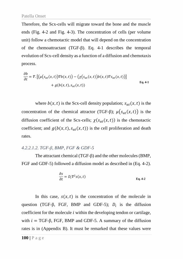
Patella Onset
100 | P a g e
Therefore, the Scx-cells will migrate toward the bone and the muscle
ends (Fig. 4-2 and Fig. 4-3). The concentration of cells (per volume
unit) follow a chemotactic model that will depend on the concentration
of the chemoattractant (TGF-β). Eq. 4-1 describes the temporal
evolution of Scx-cell density as a function of a diffusion and chemotaxis
process.
𝜕𝑏
𝜕𝑡= 𝛻. [(𝜇(𝑠𝑎𝑡(𝑥, 𝑡))𝛻𝑏(𝑥, 𝑡)) − (𝜒(𝑠𝑎𝑡(𝑥, 𝑡))𝑏(𝑥, 𝑡)𝛻𝑠𝑎𝑡(𝑥, 𝑡))]
+ 𝑔(𝑏(𝑥, 𝑡), 𝑠𝑎𝑡(𝑥, 𝑡)) Eq. 4-1
where 𝑏(𝑥, 𝑡) is the Scx-cell density population; 𝑠𝑎𝑡(𝑥, 𝑡) is the
concentration of the chemical attractor (TGF-β); 𝜇(𝑠𝑎𝑡(𝑥, 𝑡)) is the
diffusion coefficient of the Scx-cells; 𝜒(𝑠𝑎𝑡(𝑥, 𝑡)) is the chemotactic
coefficient; and 𝑔(𝑏(𝑥, 𝑡), 𝑠𝑎𝑡(𝑥, 𝑡)) is the cell proliferation and death
rates.
4.2.2.1.2. TGF-β, BMP, FGF & GDF-5
The attractant chemical (TGF-β) and the other molecules (BMP,
FGF and GDF-5) followed a diffusion model as described in (Eq. 4-2).
𝜕𝑠
𝜕𝑡= 𝐷𝑖∇
2𝑠(𝑥, 𝑡) Eq. 4-2
In this case, 𝑠(𝑥, 𝑡) is the concentration of the molecule in
question (TGF-β, FGF, BMP and GDF-5); 𝐷𝑖 is the diffusion
coefficient for the molecule 𝑖 within the developing tendon or cartilage,
with 𝑖 = TGF-β, FGF, BMP and GDF-5. A summary of the diffusion
rates is in (Appendix B). It must be remarked that these values were
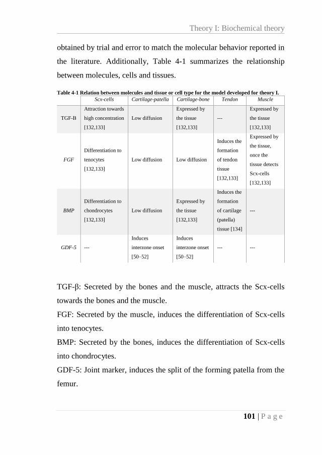
Theory I: Biochemical theory
101 | P a g e
obtained by trial and error to match the molecular behavior reported in
the literature. Additionally, Table 4-1 summarizes the relationship
between molecules, cells and tissues.
Table 4-1 Relation between molecules and tissue or cell type for the model developed for theory I.
Scx-cells Cartilage-patella Cartilage-bone Tendon Muscle
TGF-Β
Attraction towards
high concentration
[132,133]
Low diffusion
Expressed by
the tissue
[132,133]
---
Expressed by
the tissue
[132,133]
FGF
Differentiation to
tenocytes
[132,133]
Low diffusion Low diffusion
Induces the
formation
of tendon
tissue
[132,133]
Expressed by
the tissue,
once the
tissue detects
Scx-cells
[132,133]
BMP
Differentiation to
chondrocytes
[132,133]
Low diffusion
Expressed by
the tissue
[132,133]
Induces the
formation
of cartilage
(patella)
tissue [134]
---
GDF-5 ---
Induces
interzone onset
[50–52]
Induces
interzone onset
[50–52]
--- ---
TGF-β: Secreted by the bones and the muscle, attracts the Scx-cells
towards the bones and the muscle.
FGF: Secreted by the muscle, induces the differentiation of Scx-cells
into tenocytes.
BMP: Secreted by the bones, induces the differentiation of Scx-cells
into chondrocytes.
GDF-5: Joint marker, induces the split of the forming patella from the
femur.
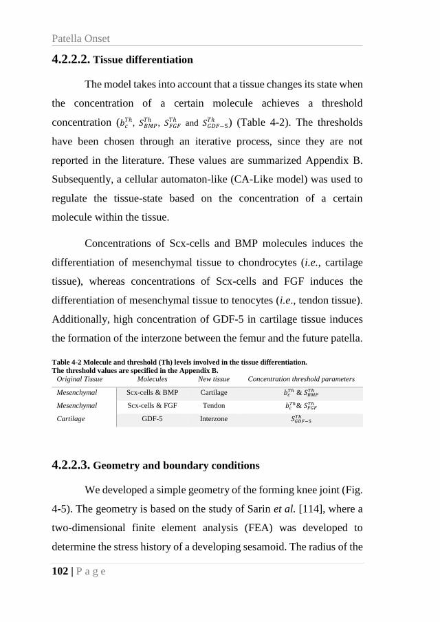
Patella Onset
102 | P a g e
4.2.2.2. Tissue differentiation
The model takes into account that a tissue changes its state when
the concentration of a certain molecule achieves a threshold
concentration (𝑏𝑐𝑇ℎ, 𝑆𝐵𝑀𝑃
𝑇ℎ , 𝑆𝐹𝐺𝐹𝑇ℎ and 𝑆𝐺𝐷𝐹−5
𝑇ℎ ) (Table 4-2). The thresholds
have been chosen through an iterative process, since they are not
reported in the literature. These values are summarized Appendix B.
Subsequently, a cellular automaton-like (CA-Like model) was used to
regulate the tissue-state based on the concentration of a certain
molecule within the tissue.
Concentrations of Scx-cells and BMP molecules induces the
differentiation of mesenchymal tissue to chondrocytes (i.e., cartilage
tissue), whereas concentrations of Scx-cells and FGF induces the
differentiation of mesenchymal tissue to tenocytes (i.e., tendon tissue).
Additionally, high concentration of GDF-5 in cartilage tissue induces
the formation of the interzone between the femur and the future patella.
Table 4-2 Molecule and threshold (Th) levels involved in the tissue differentiation.
The threshold values are specified in the Appendix B.
Original Tissue Molecules New tissue Concentration threshold parameters
Mesenchymal Scx-cells & BMP Cartilage 𝑏𝑐𝑇ℎ & 𝑆𝐵𝑀𝑃
𝑇ℎ
Mesenchymal Scx-cells & FGF Tendon 𝑏𝑐𝑇ℎ& 𝑆𝐹𝐺𝐹
𝑇ℎ
Cartilage GDF-5 Interzone 𝑆𝐺𝐷𝐹−5𝑇ℎ
4.2.2.3. Geometry and boundary conditions
We developed a simple geometry of the forming knee joint (Fig.
4-5). The geometry is based on the study of Sarin et al. [114], where a
two-dimensional finite element analysis (FEA) was developed to
determine the stress history of a developing sesamoid. The radius of the
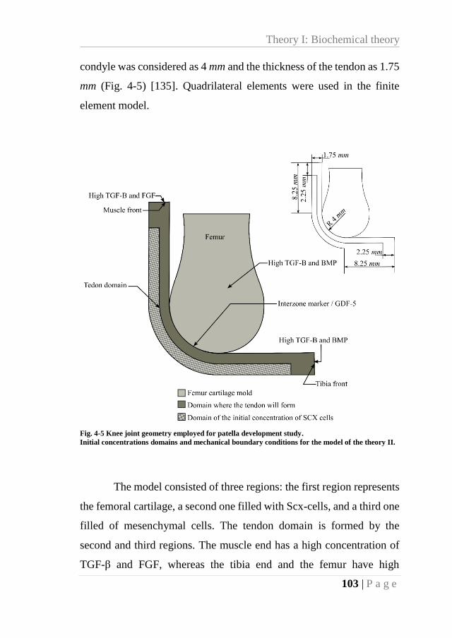
Theory I: Biochemical theory
103 | P a g e
condyle was considered as 4 mm and the thickness of the tendon as 1.75
mm (Fig. 4-5) [135]. Quadrilateral elements were used in the finite
element model.
Fig. 4-5 Knee joint geometry employed for patella development study.
Initial concentrations domains and mechanical boundary conditions for the model of the theory II.
The model consisted of three regions: the first region represents
the femoral cartilage, a second one filled with Scx-cells, and a third one
filled of mesenchymal cells. The tendon domain is formed by the
second and third regions. The muscle end has a high concentration of
TGF-β and FGF, whereas the tibia end and the femur have high
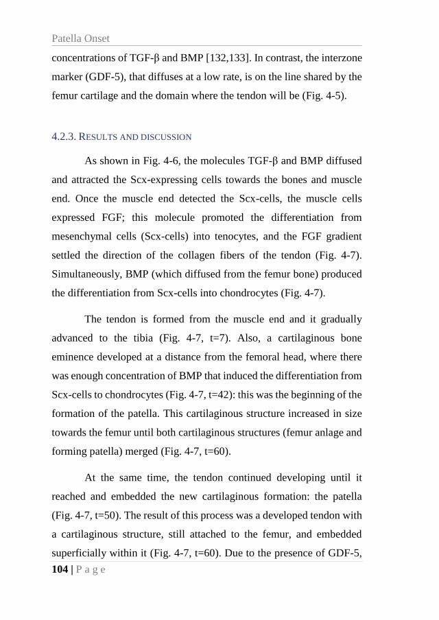
Patella Onset
104 | P a g e
concentrations of TGF-β and BMP [132,133]. In contrast, the interzone
marker (GDF-5), that diffuses at a low rate, is on the line shared by the
femur cartilage and the domain where the tendon will be (Fig. 4-5).
4.2.3. RESULTS AND DISCUSSION
As shown in Fig. 4-6, the molecules TGF-β and BMP diffused
and attracted the Scx-expressing cells towards the bones and muscle
end. Once the muscle end detected the Scx-cells, the muscle cells
expressed FGF; this molecule promoted the differentiation from
mesenchymal cells (Scx-cells) into tenocytes, and the FGF gradient
settled the direction of the collagen fibers of the tendon (Fig. 4-7).
Simultaneously, BMP (which diffused from the femur bone) produced
the differentiation from Scx-cells into chondrocytes (Fig. 4-7).
The tendon is formed from the muscle end and it gradually
advanced to the tibia (Fig. 4-7, t=7). Also, a cartilaginous bone
eminence developed at a distance from the femoral head, where there
was enough concentration of BMP that induced the differentiation from
Scx-cells to chondrocytes (Fig. 4-7, t=42): this was the beginning of the
formation of the patella. This cartilaginous structure increased in size
towards the femur until both cartilaginous structures (femur anlage and
forming patella) merged (Fig. 4-7, t=60).
At the same time, the tendon continued developing until it
reached and embedded the new cartilaginous formation: the patella
(Fig. 4-7, t=50). The result of this process was a developed tendon with
a cartilaginous structure, still attached to the femur, and embedded
superficially within it (Fig. 4-7, t=60). Due to the presence of GDF-5,
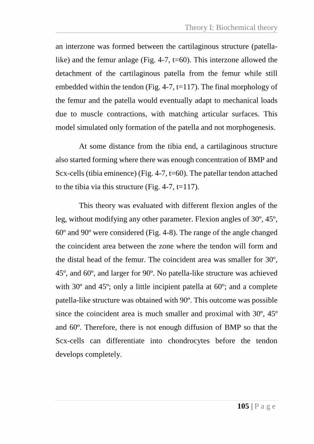
Theory I: Biochemical theory
105 | P a g e
an interzone was formed between the cartilaginous structure (patella-
like) and the femur anlage (Fig. 4-7, t=60). This interzone allowed the
detachment of the cartilaginous patella from the femur while still
embedded within the tendon (Fig. 4-7, t=117). The final morphology of
the femur and the patella would eventually adapt to mechanical loads
due to muscle contractions, with matching articular surfaces. This
model simulated only formation of the patella and not morphogenesis.
At some distance from the tibia end, a cartilaginous structure
also started forming where there was enough concentration of BMP and
Scx-cells (tibia eminence) (Fig. 4-7, t=60). The patellar tendon attached
to the tibia via this structure (Fig. 4-7, t=117).
This theory was evaluated with different flexion angles of the
leg, without modifying any other parameter. Flexion angles of 30º, 45º,
60º and 90º were considered (Fig. 4-8). The range of the angle changed
the coincident area between the zone where the tendon will form and
the distal head of the femur. The coincident area was smaller for 30º,
45º, and 60º, and larger for 90º. No patella-like structure was achieved
with 30º and 45º; only a little incipient patella at 60º; and a complete
patella-like structure was obtained with 90º. This outcome was possible
since the coincident area is much smaller and proximal with 30º, 45º
and 60º. Therefore, there is not enough diffusion of BMP so that the
Scx-cells can differentiate into chondrocytes before the tendon
develops completely.
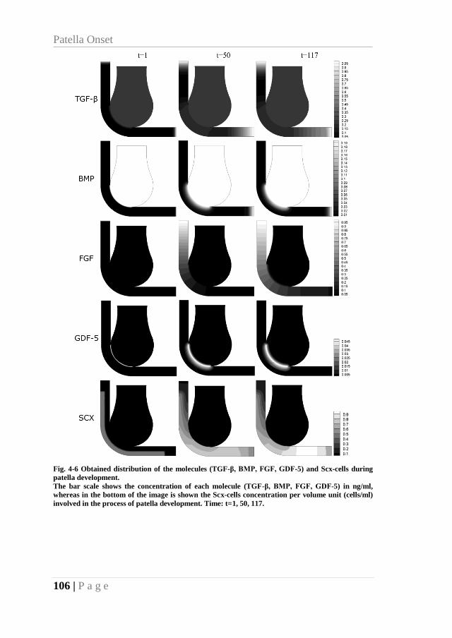
Patella Onset
106 | P a g e
Fig. 4-6 Obtained distribution of the molecules (TGF-β, BMP, FGF, GDF-5) and Scx-cells during
patella development.
The bar scale shows the concentration of each molecule (TGF-β, BMP, FGF, GDF-5) in ng/ml,
whereas in the bottom of the image is shown the Scx-cells concentration per volume unit (cells/ml)
involved in the process of patella development. Time: t=1, 50, 117.
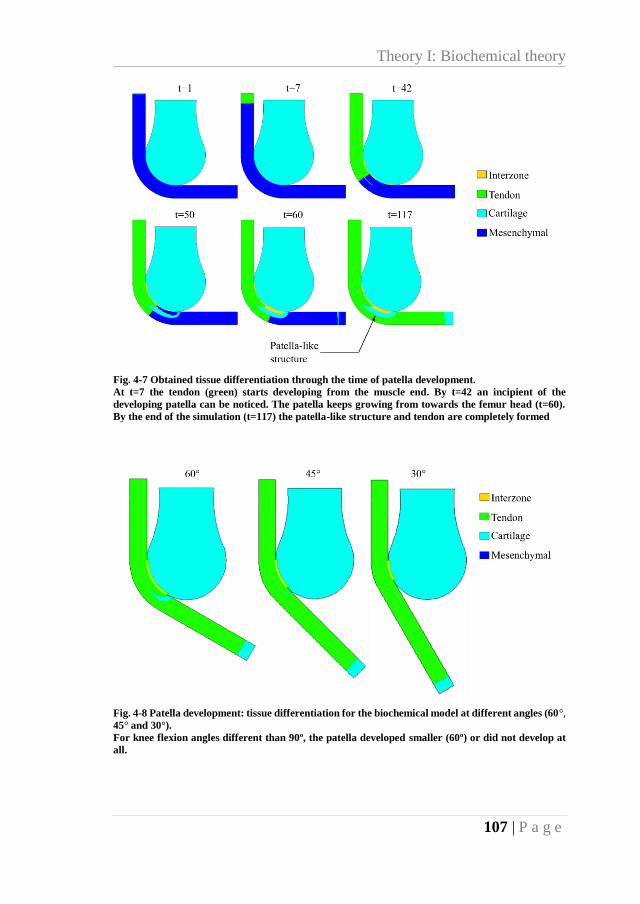
Theory I: Biochemical theory
107 | P a g e
Fig. 4-7 Obtained tissue differentiation through the time of patella development.
At t=7 the tendon (green) starts developing from the muscle end. By t=42 an incipient of the
developing patella can be noticed. The patella keeps growing from towards the femur head (t=60).
By the end of the simulation (t=117) the patella-like structure and tendon are completely formed
Fig. 4-8 Patella development: tissue differentiation for the biochemical model at different angles (60°,
45° and 30°).
For knee flexion angles different than 90º, the patella developed smaller (60º) or did not develop at
all.
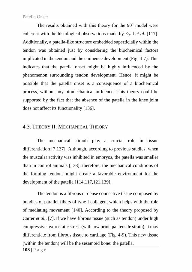
Patella Onset
108 | P a g e
The results obtained with this theory for the 90º model were
coherent with the histological observations made by Eyal et al. [117].
Additionally, a patella-like structure embedded superficially within the
tendon was obtained just by considering the biochemical factors
implicated in the tendon and the eminence development (Fig. 4-7). This
indicates that the patella onset might be highly influenced by the
phenomenon surrounding tendon development. Hence, it might be
possible that the patella onset is a consequence of a biochemical
process, without any biomechanical influence. This theory could be
supported by the fact that the absence of the patella in the knee joint
does not affect its functionality [136].
4.3. THEORY II: MECHANICAL THEORY
The mechanical stimuli play a crucial role in tissue
differentiation [7,137]. Although, according to previous studies, when
the muscular activity was inhibited in embryos, the patella was smaller
than in control animals [138]; therefore, the mechanical conditions of
the forming tendons might create a favorable environment for the
development of the patella [114,117,121,139].
The tendon is a fibrous or dense connective tissue composed by
bundles of parallel fibers of type I collagen, which helps with the role
of mediating movement [140]. According to the theory proposed by
Carter et al., [7], if we have fibrous tissue (such as tendon) under high
compressive hydrostatic stress (with low principal tensile strain), it may
differentiate from fibrous tissue to cartilage (Fig. 4-9). This new tissue
(within the tendon) will be the sesamoid bone: the patella.
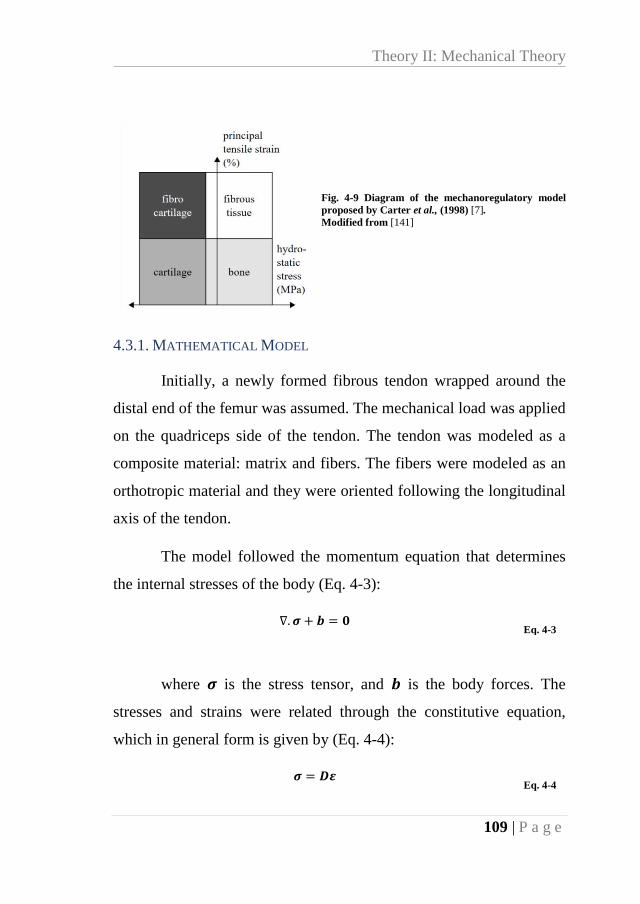
Theory II: Mechanical Theory
109 | P a g e
Fig. 4-9 Diagram of the mechanoregulatory model
proposed by Carter et al., (1998) [7].
Modified from [141]
4.3.1. MATHEMATICAL MODEL
Initially, a newly formed fibrous tendon wrapped around the
distal end of the femur was assumed. The mechanical load was applied
on the quadriceps side of the tendon. The tendon was modeled as a
composite material: matrix and fibers. The fibers were modeled as an
orthotropic material and they were oriented following the longitudinal
axis of the tendon.
The model followed the momentum equation that determines
the internal stresses of the body (Eq. 4-3):
∇. 𝝈 + 𝒃 = 𝟎 Eq. 4-3
where 𝝈 is the stress tensor, and 𝒃 is the body forces. The
stresses and strains were related through the constitutive equation,
which in general form is given by (Eq. 4-4):
𝝈 = 𝑫𝜺 Eq. 4-4
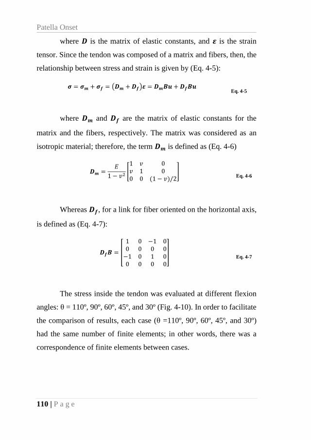
Patella Onset
110 | P a g e
where 𝑫 is the matrix of elastic constants, and 𝜺 is the strain
tensor. Since the tendon was composed of a matrix and fibers, then, the
relationship between stress and strain is given by (Eq. 4-5):
𝝈 = 𝝈𝒎 + 𝝈𝒇 = (𝑫𝒎 +𝑫𝒇)𝜺 = 𝑫𝒎𝑩𝒖 + 𝑫𝒇𝑩𝒖 Eq. 4-5
where 𝑫𝒎 and 𝑫𝒇 are the matrix of elastic constants for the
matrix and the fibers, respectively. The matrix was considered as an
isotropic material; therefore, the term 𝑫𝒎 is defined as (Eq. 4-6)
𝑫𝒎 =𝐸
1 − 𝑣2[1 𝑣 0𝑣 1 00 0 (1 − 𝑣)/2
] Eq. 4-6
Whereas 𝑫𝒇, for a link for fiber oriented on the horizontal axis,
is defined as (Eq. 4-7):
𝑫𝒇𝑩 = [
1 0 −1 00 0 0 0−1 0 1 00 0 0 0
] Eq. 4-7
The stress inside the tendon was evaluated at different flexion
angles: θ = 110º, 90º, 60º, 45º, and 30º (Fig. 4-10). In order to facilitate
the comparison of results, each case (θ =110º, 90º, 60º, 45º, and 30º)
had the same number of finite elements; in other words, there was a
correspondence of finite elements between cases.
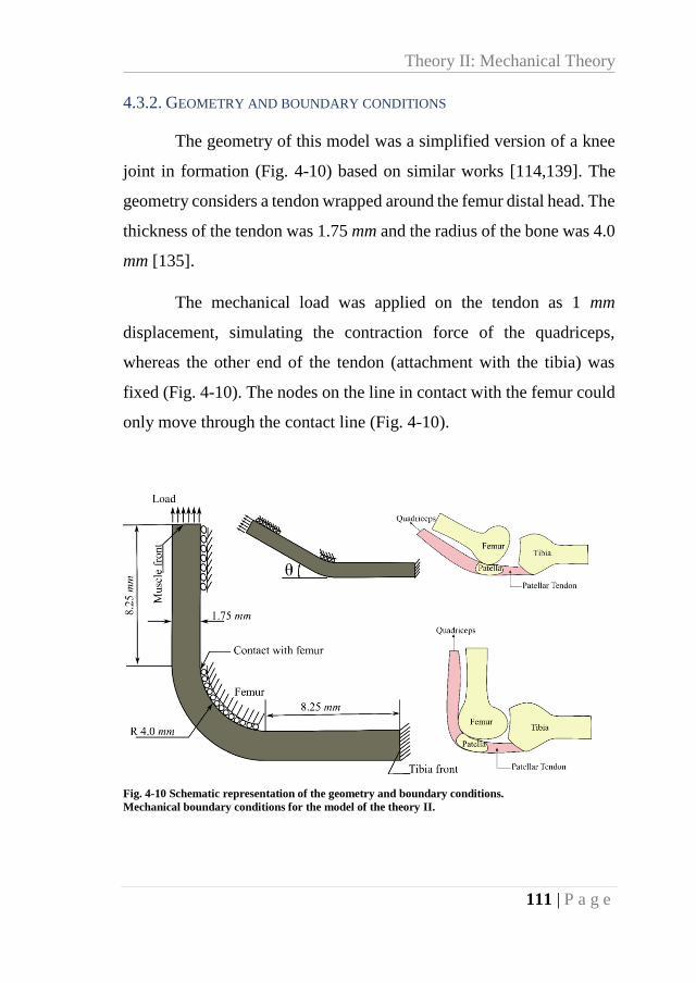
Theory II: Mechanical Theory
111 | P a g e
4.3.2. GEOMETRY AND BOUNDARY CONDITIONS
The geometry of this model was a simplified version of a knee
joint in formation (Fig. 4-10) based on similar works [114,139]. The
geometry considers a tendon wrapped around the femur distal head. The
thickness of the tendon was 1.75 mm and the radius of the bone was 4.0
mm [135].
The mechanical load was applied on the tendon as 1 mm
displacement, simulating the contraction force of the quadriceps,
whereas the other end of the tendon (attachment with the tibia) was
fixed (Fig. 4-10). The nodes on the line in contact with the femur could
only move through the contact line (Fig. 4-10).
Fig. 4-10 Schematic representation of the geometry and boundary conditions.
Mechanical boundary conditions for the model of the theory II.
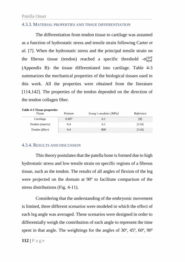
Patella Onset
112 | P a g e
4.3.3. MATERIAL PROPERTIES AND TISSUE DIFFERENTIATION
The differentiation from tendon tissue to cartilage was assumed
as a function of hydrostatic stress and tensile strain following Carter et
al. [7]. When the hydrostatic stress and the principal tensile strain on
the fibrous tissue (tendon) reached a specific threshold -σhydcart
(Appendix B)- the tissue differentiated into cartilage. Table 4-3
summarizes the mechanical properties of the biological tissues used in
this work. All the properties were obtained from the literature
[114,142]. The properties of the tendon depended on the direction of
the tendon collagen fiber.
Table 4-3 Tissue properties
Tissue Poisson Young’s modulus [MPa] Reference
Cartilage 0.497 6.1 [8]
Tendon (matrix) 0.4 6.1 [114]
Tendon (fiber) 0.4 800 [114]
4.3.4. RESULTS AND DISCUSSION
This theory postulates that the patella bone is formed due to high
hydrostatic stress and low tensile strain on specific regions of a fibrous
tissue, such as the tendon. The results of all angles of flexion of the leg
were projected on the domain at 90º to facilitate comparison of the
stress distributions (Fig. 4-11).
Considering that the understanding of the embryonic movement
is limited, three different scenarios were modeled in which the effect of
each leg angle was averaged. These scenarios were designed in order to
differentially weigh the contribution of each angle to represent the time
spent in that angle. The weightings for the angles of 30º, 45º, 60º, 90º
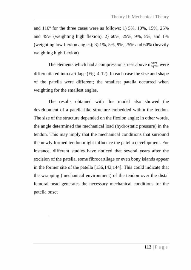
Theory II: Mechanical Theory
113 | P a g e
and 110º for the three cases were as follows: 1) 5%, 10%, 15%, 25%
and 45% (weighting high flexion), 2) 60%, 25%, 9%, 5%, and 1%
(weighting low flexion angles); 3) 1%, 5%, 9%, 25% and 60% (heavily
weighting high flexion).
The elements which had a compression stress above σhydcart, were
differentiated into cartilage (Fig. 4-12). In each case the size and shape
of the patella were different; the smallest patella occurred when
weighting for the smallest angles.
The results obtained with this model also showed the
development of a patella-like structure embedded within the tendon.
The size of the structure depended on the flexion angle; in other words,
the angle determined the mechanical load (hydrostatic pressure) in the
tendon. This may imply that the mechanical conditions that surround
the newly formed tendon might influence the patella development. For
instance, different studies have noticed that several years after the
excision of the patella, some fibrocartilage or even bony islands appear
in the former site of the patella [136,143,144]. This could indicate that
the wrapping (mechanical environment) of the tendon over the distal
femoral head generates the necessary mechanical conditions for the
patella onset
.
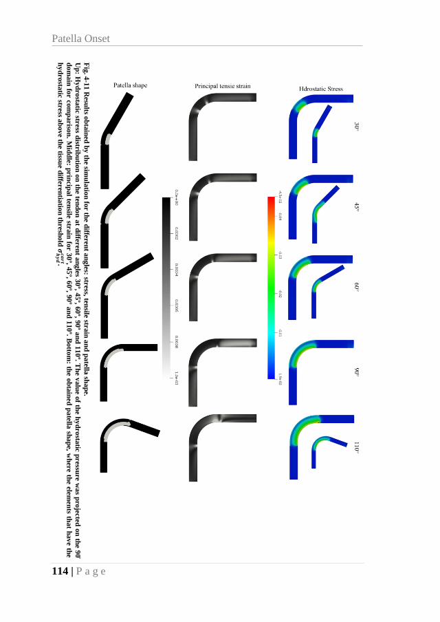
Patella Onset
114 | P a g e
Fig
. 4-1
1 R
esults o
bta
ined
by
the sim
ula
tion
for th
e d
iffere
nt a
ng
les: str
ess, te
nsile
strain
an
d p
ate
lla sh
ap
e.
Up
: Hy
dro
static str
ess d
istrib
utio
n o
n th
e ten
do
n a
t diffe
ren
t an
gle
s 30
º, 45
º, 60
º, 90
º an
d 1
10
º. Th
e valu
e of th
e hy
dro
static
pressu
re w
as p
roje
cte
d o
n th
e 9
0̊
do
ma
in fo
r c
om
pariso
n. M
idd
le: p
rin
cipal te
nsile str
ain
for 3
0º, 4
5º, 6
0º, 9
0º a
nd
110
º. Bo
ttom
: the o
bta
ined
pa
tella
sha
pe, w
here
the e
lem
en
ts tha
t hav
e th
e
hy
dro
static
stress a
bove th
e tissu
e d
ifferen
tiatio
n th
resh
old
𝝈𝒉𝒚𝒅
𝒄𝒂𝒓𝒕.
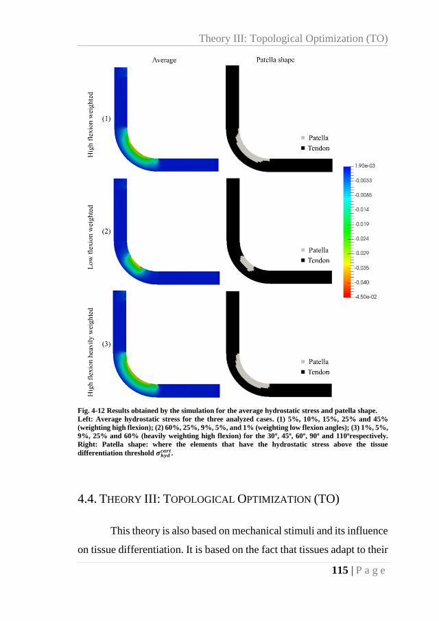
Theory III: Topological Optimization (TO)
115 | P a g e
Fig. 4-12 Results obtained by the simulation for the average hydrostatic stress and patella shape.
Left: Average hydrostatic stress for the three analyzed cases. (1) 5%, 10%, 15%, 25% and 45%
(weighting high flexion); (2) 60%, 25%, 9%, 5%, and 1% (weighting low flexion angles); (3) 1%, 5%,
9%, 25% and 60% (heavily weighting high flexion) for the 30º, 45º, 60º, 90º and 110ºrespectively.
Right: Patella shape: where the elements that have the hydrostatic stress above the tissue
differentiation threshold 𝝈𝒉𝒚𝒅𝒄𝒂𝒓𝒕.
4.4. THEORY III: TOPOLOGICAL OPTIMIZATION (TO)
This theory is also based on mechanical stimuli and its influence
on tissue differentiation. It is based on the fact that tissues adapt to their
Patella Onset
116 | P a g e
stress and strain environment; therefore, TO might be suitable to
explain this adaptation. TO can be applied in tissue remodeling, since it
iteratively redistributes the material in a design domain determining an
optimal material arrangement or tissue type [125]. Specifically, TO
allocates denser material (cartilage) to regions under relatively high
strain energy and allocates a less dense material (tendon) to zones with
a low strain energy. This adaptation process can be characterized as a
self-enhancing system [122], with the objective of minimizing tendon
strain. Therefore, articular surface wear will be reduced due to the low
relative movement between the distal femoral head joint surface and the
tendon.
As an initial condition, it was considered that the tendon was
already formed and loaded. A two-dimensional FEA analysis based on
the algorithm proposed on Sigmund [145], was performed. The
algorithm is based on the “power-law approach” or SIMP approach
(Solid Isotropic Material with Penalization) [145]. This approach
assumes that the material properties are constant within each element
of the design domain, whereas the relative material densities of the
elements are the variables [145]. The density is usually considered as a
design variable, so it could take values between 0 and 1, with 0
representing void and 1 representing solid [146]. Thus, the relation
between the elastic modulus and the relative material density is given
in Eq. 4-8:
𝐸(𝑥) = 𝜌(𝑥)𝑝𝐸𝑜 Eq. 4-8
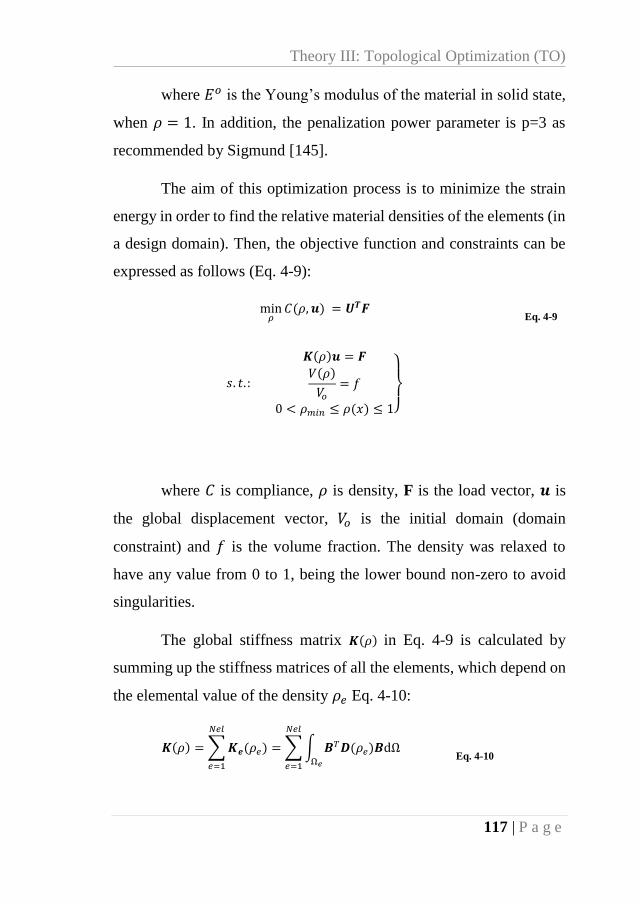
Theory III: Topological Optimization (TO)
117 | P a g e
where 𝐸𝑜 is the Young’s modulus of the material in solid state,
when 𝜌 = 1. In addition, the penalization power parameter is p=3 as
recommended by Sigmund [145].
The aim of this optimization process is to minimize the strain
energy in order to find the relative material densities of the elements (in
a design domain). Then, the objective function and constraints can be
expressed as follows (Eq. 4-9):
min𝜌𝐶(𝜌, 𝒖) = 𝑼𝑻𝑭
Eq. 4-9
𝑠. 𝑡. :
𝑲(𝜌)𝒖 = 𝑭
𝑉(𝜌)
𝑉𝑜= 𝑓
0 < 𝜌𝑚𝑖𝑛 ≤ 𝜌(𝑥) ≤ 1}
where 𝐶 is compliance, 𝜌 is density, F is the load vector, 𝒖 is
the global displacement vector, 𝑉𝑜 is the initial domain (domain
constraint) and 𝑓 is the volume fraction. The density was relaxed to
have any value from 0 to 1, being the lower bound non-zero to avoid
singularities.
The global stiffness matrix 𝑲(𝜌) in Eq. 4-9 is calculated by
summing up the stiffness matrices of all the elements, which depend on
the elemental value of the density 𝜌𝑒 Eq. 4-10:
𝑲(𝜌) =∑𝑲𝒆(𝜌𝑒)
𝑁𝑒𝑙
𝑒=1
=∑∫ 𝑩𝑇𝑫(𝜌𝑒)𝑩dΩΩ𝑒
𝑁𝑒𝑙
𝑒=1
Eq. 4-10

Patella Onset
118 | P a g e
where 𝑲𝒆(𝜌𝑒) is the stiffness matrix of the element, 𝑩 is the
shape function derivatives, and 𝑫(𝝆𝒆) is the constitutive matrix which
depends on the material density. Sensitivities of the objective function
and volume constraint with respect to 𝜌𝑒 are calculated as follows (Eq.
4-11 and Eq. 4-12):
𝜕𝐶
𝜕𝜌𝑒= −𝒖𝑒
𝑇𝜕𝑲𝒆
𝜕𝜌𝑒𝒖𝑒 = −𝑝𝜌𝑒
𝑝−1𝒖𝑒𝑇𝑲𝑒
𝑜𝒖𝑒 Eq. 4-11
𝜕𝑉
𝜕𝜌𝑒= ∫ d𝑉
Ωe
Eq. 4-12
A heuristic updating scheme for the design variable is
formulated as (Eq. 4-13):
𝜌𝑒𝑛𝑒𝑤 = {
max(𝜌𝑚𝑖𝑛 , 𝜌𝑒 −𝑚) 𝑖𝑓 𝜌𝑒𝐵𝑒𝜂≤ max(𝜌𝑚𝑖𝑛 , 𝜌𝑒 −𝑚) ,
𝜌𝑒𝐵𝑒𝜂 𝑖𝑓 max(𝜌𝑚𝑖𝑛, 𝜌𝑒 −𝑚) < 𝜌𝑒𝐵𝑒
𝜂< min(1, 𝜌𝑒 +𝑚) ,
min(1, 𝜌𝑒 +𝑚) 𝑖𝑓 min(1, 𝜌𝑒 −𝑚) ≤ 𝜌𝑒𝐵𝑒𝜂,
Eq. 4-13
where m is a positive moving limit, 𝜂 is the numerical damping
coefficient and 𝐵𝑒 is the optimality condition which is calculated as (Eq.
4-14):
𝐵𝑒 =
𝜕𝐶𝜕𝜌𝑒
𝜆𝜕𝑉𝜕𝜌𝑒
Eq. 4-14
4.4.1. GEOMETRY AND BOUNDARY CONDITIONS
The same geometry and boundary conditions of Theory II
(Theory II: Geometry and boundary conditions) were used in this
model.
Theory III: Topological Optimization (TO)
119 | P a g e
4.4.2. MATERIAL PROPERTIES
The tissue properties of the initial domain (tendon and fibers)
are summarized in (Table 4-3) (Theory II: Material properties and tissue
differentiation). The properties of the tendon depended on the direction
of the tendon collagen fibers.
4.4.3. RESULTS AND DISCUSSION
In this third theory, the appearance of the patella is due to a TO
process in the recently formed patellar tendon. Different angles were
tested for this model; however, we only obtained coherent results
(formed patella) with 90º and 110º. For these angles, we observed a
high-density zone close to the usual patella position. Specifically, for
the 90º case, the shape of the high-density zone is more consistent with
reality (Fig. 4-13). This suggests that the mechanical environment that
surrounds the tendon may affect the patella and its development.
Some studies have uncovered that quite a long while after the
extraction of the patella, islands of fibrocartilage, or even bone show up
in the previous site of the patella. [143,144]. These islands might be the
result of the optimization process that the human body undergoes due
to the abnormal conditions after the patella excision. The strain energy
is reduced in this process, which allows the tendon to have small
displacements and deformations.
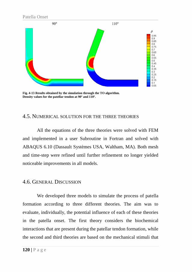
Patella Onset
120 | P a g e
Fig. 4-13 Results obtained by the simulation through the TO algorithm.
Density values for the patellar tendon at 90º and 110º.
4.5. NUMERICAL SOLUTION FOR THE THREE THEORIES
All the equations of the three theories were solved with FEM
and implemented in a user Subroutine in Fortran and solved with
ABAQUS 6.10 (Dassault Systèmes USA, Waltham, MA). Both mesh
and time-step were refined until further refinement no longer yielded
noticeable improvements in all models.
4.6. GENERAL DISCUSSION
We developed three models to simulate the process of patella
formation according to three different theories. The aim was to
evaluate, individually, the potential influence of each of these theories
in the patella onset. The first theory considers the biochemical
interactions that are present during the patellar tendon formation, while
the second and third theories are based on the mechanical stimuli that
General Discussion
121 | P a g e
the newly developed patellar tendon goes through. All three models
used a simplified knee geometry, considering both the tendon and the
femur for the biochemical-based theory (Fig. 4-5), and only the tendon
for the mechanical-based theories; the femur was assumed as a rigid
body.
The biochemical model is a conceptual model of the
development of the patella based on the theory proposed by Eyal et al.
[117], where the patella initially forms as a bone eminence, involving
Scx-cells whose differentiation is regulated by TGF-β and BMP-4. The
separation of the patella from the femur is regulated through the
interzone molecule GDF-5. The simulated molecular distribution
agrees with that previously shown [117], where at the end a patella-like
structure embedded superficially within the tendon was obtained. We
assumed the diffusion rates of the molecules based on an iterative
process, since they are not reported in the literature and are particularly
difficult to measure.
Additionally, we also simulated the biochemical model when
the leg was extended at different angles (30º, 45º, 60º, 90º). The latter
was to establish how the position of the leg affected the development of
the patella, in the case that only biochemical factors influenced the
formation of this sesamoid bone. When the angles of the leg were
modified to 30º, 45º or 60º, the region through which BMP diffused
from the femur distal end to the tendon region was smaller.
Consequently, the patella obtained was either not significant or null
(Fig. 4-8). This may be evidence, according to this theory, that having
an angle close to 90º is necessary to form the patella.

Patella Onset
122 | P a g e
On the other hand, the first mechanical model is based on the
theories which state that mechanical stimuli play a crucial role in tissue
differentiation. Particularly, this model is built upon Carter’s theory [7],
in which hydrostatic compression and low principal strain are stimuli
that induce fibrous tissue differentiation into cartilage. It was assumed
that the constant movements of the fetus (distinct knee angles) stimulate
the concentration of high compression loads on some areas of the newly
formed tendon. The latter induces the differentiation of the tendon cells
into cartilage, on those high hydrostatic stress zones. Therefore, a
cartilage structure is formed embedded within the tendon, which later
will ossify and become the patella bone.
Following this last theory (the mechano-differentiation model),
a patella-like structure was obtained. When different flexion angles of
the leg were evaluated, we observed an influence on the size of the
patella (Fig. 4-11). Additionally, a patella-like structure was obtained
when the hydrostatic stress was averaged considering all the angles. A
different predominant angle for each case was evaluated: weighting
high flexion, weighting low flexion angles and heavily weighting high
flexion. If the predominant angle was large, a big patella was obtained,
whereas if the predominant angle was small, a short patella was
obtained (Fig. 4-12).
The last evaluated theory was based on the application of TO,
which is also feasible to explain the onset of sesamoid bones such as
the patella. In this case, we assume that the tissue can adapt to its
mechanical environment in a way that its strain energy is reduced.
Different angles were also evaluated. However, the outcome was not as

General Discussion
123 | P a g e
expected for smaller angles since no patella-like structure was obtained.
Nevertheless, a patella-like structure was achieved with angles of 90º
and 110º. The shape of the obtained patella is remarkably similar,
especially with an angle of 90º. The results of this model imply that the
patella might allow reducing the strain energy and, consequently, the
displacements and deformations of the tendon. These results also imply
that the patella and the femur articular surface have a low relative
movement. This is due to the low deformation of the tendon, protecting
somehow the femur articular surface from wear.
A patella-like structure was obtained for most of the knee
flexion angles in all the theories we have evaluated. Our results show
that tissue remodeling and adaption, based on Carter’s theory or on TO,
could be responsible for the patella onset. The shape, position and size
of the patella would depend on the flexion angle of the leg, and the time
that the leg spends on each position, obtaining a larger-sized patella
compared to the biochemical approach. However, there is not much
evidence in the literature that can support the second and third theories.
Some studies have shown that while limitation of movement (through
drugs) on embryos affects the formation of the patella, it develops
anyway, although small in size [138]. Therefore, the mechanical load
may not be necessary for the appearance of the patella, but it may be
necessary for its morphogenesis and maintenance. Hence, molecular
factors and their interactions trigger the formation of the patella, as
evidenced by molecular expression analyzed in histological slides
[117]. These factors, applied through a computational model, were
consistent with the results we obtained. However, since only the
Patella Onset
124 | P a g e
limitation of the movement does not guarantee that there are no
hydrostatic stresses on the tendon, more tests should be run in which
only biochemical factors influence the development of the tendon and
the patella. It is also possible that these mechanisms are redundant and
that both influence the patella onset
This study proposes a simplified mathematical model of the
regulatory mechanisms that might influence the formation of the patella
bone. Each theory was evaluated separately to observe its outcome and
the likelihood of its influence on the patella onset. The results obtained
were consistent, and patella-like structures were obtained in most cases.
Nevertheless, the literature suggests that the patella onset could be
triggered by biochemical factors during tendon development [117];
according to our results, this approach does lead to a patella-like
structure. Also, it is certain that the mechanical environment must affect
the patella development. However, this environment might affect it
mostly after the tendon is formed by helping the patella to obtain its
final shape and maintain its structure.
This work is a first approximation on understanding the process
of the development of the patella. It should be considered that these
models had several simplifications, such as that they were all two-
dimensional models, that the geometry was a simplified knee joint, that
all the materials were modeled as linear elastic, and that the molecular
concentrations, since they are difficult to measure and there are no
reports in literature, were established through an iterative process. Even
though of the simplifications, we obtained results that might explain the
onset of the patella and would help in the proposition of new points of
General Discussion
125 | P a g e
view that might explain the patella onset. Furthermore, these models
could provide new insight and guidelines of experimentation, and of
course, new mathematical models as well. However, a combination of
the theories evaluated in this study is suggested for future works, so that
the patella onset is determined due to biochemical factors, and
thereafter the mechanical loads may regulate its shape and maintenance.
The exact instant and way that mechanical loads affect the patella
development should be an issue to evaluate in further models, as well
as the dynamic movement of the knee during the development.

127 | P a g e
Chapter 5. CARTILAGE
REGENERATION
5.1. INTRODUCTION
Articular cartilage has a limited ability to repair itself, therefore,
it is common to find pathologies related to articular cartilage injuries or
aging. This may be since the articular cartilage is an avascular tissue
and has a low capacity to regenerate itself. Hence, in a lesion of the
articular cartilage, a scar composed mainly of fibrocartilage is
frequently generated, which is a tissue with mechanical properties
inferior to hyaline cartilage that degrades over time [1,147].
Lesions in the articular cartilage have different causes such as
intra-articular fracture, progressive degradation of OA, or
osteochondritis dissecans, among others [3,148,149]. Lately, the
damage that suffers the subchondral bone has received increasing
interest for its role in joint injury, since changes of properties of the
subchondral bone seems to mediate changes observed in OA, e.g.
sclerosis reduces the shock-absorbing capability of the subchondral
bone and increases the risk of shear-induced tensile failure of the
articular cartilage [29]. Moreover, due to the rich vascularization and
innervation of the subchondral bone, it is a source of inflammatory
mediators, which are associated with the degradation of deeper layers
of articular cartilage [29]. On the architectural level, can be observed

Cartilage regeneration
128 | P a g e
the emerging of microcracks within the subchondral bone, encourage
the rapid bone remodeling as an excessive bone formation, which may
result in bone sclerosis.
Proposed treatments for OA range from symptomatic, with
analgesics and anti-inflammatory, to more invasive ones that not always
can be used or have no good results, e.g., microfracture, endochondral
transplantation, periosteum or perichondrium, cellular transplantation
(chondrocytes or stem cells); being the last resort arthrodesis
treatments, or total replacement of the joint [150]. In any case, it is
preferable not to reach the last resort and to preserve the original
function of the joint through the regeneration of the articular cartilage
rather than the replacement of the joint or an arthrodesis, especially in
young patients.
The osteochondral grafts is the most effective of the articular
cartilage regeneration treatments [1,2]. Being an autologous implant,
this treatment avoids the immunity response [1]. However, these grafts
have disadvantages: patients must go through two surgeries, new
defects are created, they are not appropriate to treat large articular
defects, they do not fuse with the adjacent articular cartilage therefore
they become unstable with time, and normally the new tissue is
fibrocartilage and not hyaline cartilage [1]. In the end, 10-20% of cases
need to be re-operated in the short term, and the percentage increases in
the long term [2].
The articular cartilage degenerative problem is part of the scope
of tissue engineering. It is necessary to search for clinical advances in
cartilage regeneration, which are less invasive, in both mild and acute
Introduction
129 | P a g e
joint injuries. In tissues such as bone or skin, repair techniques have
been based on the use of implants obtaining good results [3]. In
cartilage, based on the same techniques, they have used scaffolds,
which have gained attention in the last two decades [3]. The scaffolds
allow rapid filling of joint defects, providing a substrate where cells can
anchor, while maintaining mechanical integrity.
More recently, the scaffold technic involves three mayor
components: scaffold materials, cell proliferation or differentiation
factors, and cellular sources [3]. Scaffolds can be made of both natural
(e.g., collagen) and synthetic materials [1,4,147,151–157]. Concerning
the chondro-inductive growth factors, members of the TGF-β, insulin-
like growth factor-1 (IGF-1) and specific members FGF family are
considered. [1,3,157]. Regarding cellular sources, they include isolated
autologous chondrocytes, multipotent stem cells, pluripotent stem cells
and induced pluripotent stem cells [1,3,157]; however, scaffolds can
also be used without cellular sources [4,147,158–160].
The use of scaffolds has the advantage that it facilitates the
implant process being a less invasive process than the autologous
osteochondral grafts [147]. However, it is difficult to replicate in a
scaffold the specific conditions of the ECM [1,161]. Moreover,
manufacture scaffolds with biophysical, biochemical, and structural
characteristics similar to those of articular cartilage is a challenging
problem [1,162]. Nevertheless, great steps have been taken in the
development of biomaterials allowing them to maintain their integrity
and support the mechanical loads to which the cartilage is subjected, in
Cartilage regeneration
130 | P a g e
this way, these biomaterials are capable of imitating the characteristics
of healthy tissues [147,160,163,164].
Since 2010, researchers have increased the use of scaffolds
without a cellular source [160]. The latter method has shown results
similar to the scaffold/cell method, avoiding risks associated with cell
manipulation (contamination of bacteria and phenotype loss during
handling), and reduced costs [158–160,165,166].
Previous work in our group showed that when scaffolds/cell-
free implants were used in a rabbit experimental model, hyaline
cartilage was generated in the upper part of the scaffold by the third
month after implantation [4,158,167]. The rapid growth of the
superficial layer of the cartilage covered the scaffold while it was
displaced to the subchondral bone [4]. The role of scaffolds is to ensure
a propitious mechanical environment, which is an important factor to
activate mechanisms of cellular proliferation and differentiation to
chondrocytes [158,163]; mechanical feedback determines the behavior
of cells on its shape, migration, division, differentiation and death
[168]. It is in this mechanical relationship that computational models
contribute to the study of the biomechanical environment of
chondrocytes, evaluating difficult-to-reach aspects for experimental
models [5]. In this way, computational models can provide a
quantitative and qualitative evaluation of mechanobiological
interactions while being fed with clinical or experimental parameters
[6].
The biological computational models have been very useful to
simulate pathologies, repair and recovery of tissues and organs, e.g.,
Materials and methods
131 | P a g e
bone regeneration [7], bone growth [8], pattern formation [9–15],
embryonic development [16], among others. For cartilage, various
computational models have been developed for the articular cartilage of
the knee [17–19] and the mechanobiology of articular cartilage under
compression in confinement conditions [5]. Likewise, computational
models have been evaluated to simulate the behavior of chondrocytes
in 3D constructs [169–171], and the variables that should include the
computational models of articular cartilage [18,116,163,172–175].
Taking into account the above, our interest is to propose and
develop a simulation tool to predict the results of implanting polymer
scaffolds within a defect in the articular cartilage, in order to evaluate
their weaknesses and advantages. In this way, a deeper understanding
of the processes involved in the regeneration of articular cartilage could
be achieved. This computational model would provide insights into
how this process develops and determine the appropriate mechanical
conditions for cartilage regeneration, that can be difficult to obtain
through experimental techniques.
5.2. MATERIALS AND METHODS
5.2.1. GEOMETRY AND MESH
A plain strain axisymmetric 2D geometry was developed to
represent a simplify cartilage/bone/scaffold structure (Fig. 5-1). The
total width of the domain was considered as 36 mm, large enough to
prevent that the effect of the boundary conditions would not affect the
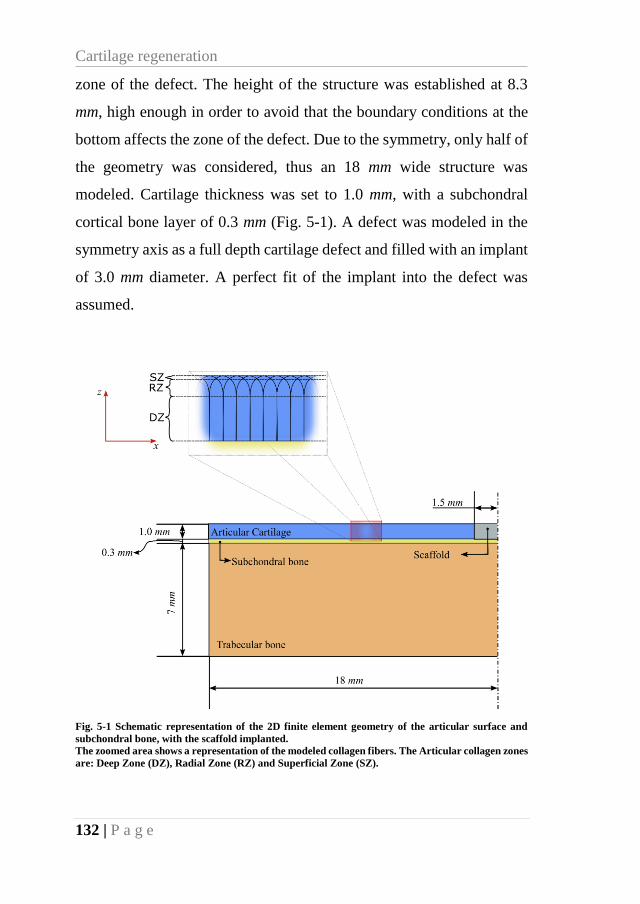
Cartilage regeneration
132 | P a g e
zone of the defect. The height of the structure was established at 8.3
mm, high enough in order to avoid that the boundary conditions at the
bottom affects the zone of the defect. Due to the symmetry, only half of
the geometry was considered, thus an 18 mm wide structure was
modeled. Cartilage thickness was set to 1.0 mm, with a subchondral
cortical bone layer of 0.3 mm (Fig. 5-1). A defect was modeled in the
symmetry axis as a full depth cartilage defect and filled with an implant
of 3.0 mm diameter. A perfect fit of the implant into the defect was
assumed.
Fig. 5-1 Schematic representation of the 2D finite element geometry of the articular surface and
subchondral bone, with the scaffold implanted.
The zoomed area shows a representation of the modeled collagen fibers. The Articular collagen zones
are: Deep Zone (DZ), Radial Zone (RZ) and Superficial Zone (SZ).
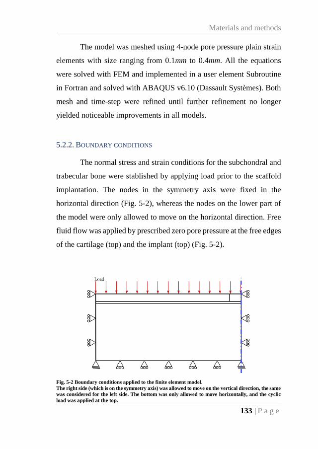
Materials and methods
133 | P a g e
The model was meshed using 4-node pore pressure plain strain
elements with size ranging from 0.1mm to 0.4mm. All the equations
were solved with FEM and implemented in a user element Subroutine
in Fortran and solved with ABAQUS v6.10 (Dassault Systèmes). Both
mesh and time-step were refined until further refinement no longer
yielded noticeable improvements in all models.
5.2.2. BOUNDARY CONDITIONS
The normal stress and strain conditions for the subchondral and
trabecular bone were stablished by applying load prior to the scaffold
implantation. The nodes in the symmetry axis were fixed in the
horizontal direction (Fig. 5-2), whereas the nodes on the lower part of
the model were only allowed to move on the horizontal direction. Free
fluid flow was applied by prescribed zero pore pressure at the free edges
of the cartilage (top) and the implant (top) (Fig. 5-2).
Fig. 5-2 Boundary conditions applied to the finite element model.
The right side (which is on the symmetry axis) was allowed to move on the vertical direction, the same
was considered for the left side. The bottom was only allowed to move horizontally, and the cyclic
load was applied at the top.
Cartilage regeneration
134 | P a g e
A unitary load was uniformly applied on the top of the cartilage.
The load was applied as an oscillatory load with 1 Hz frequency until
the values of fluid velocity (FV), stress and strain stabilize. It was
assumed that the cartilage experiences this load each day of simulation.
5.2.3. MATERIAL MODELS
5.2.3.1. Cartilage Model
Articular cartilage consists of ECM divided into two phases:
solid and fluid. The solid part contains mainly the ground substance that
includes glycoprotein and proteoglycans (PGs) anchored to hyaluronic
acid, and a fibrillar network made of collagen (type II) [176].
The mechanical response of the cartilage is highly influenced by
its tissue composition and structure [177,178]. The collagen fibrillar
network stabilizes the matrix expansion [177], and supports tension
loads, but it has low resistance for compression due to its skinniness
[176].
The collagen network is composed by a combination of large
primary collagen fibrils and smaller ad disorganized secondary fibrils.
For simplicity and computational savings, only the primary fibers were
considered. As Benninghoff described (1925) [179], bundles of primary
fibrils extend perpendicular from the subchondral bone, curving up
close to the surface and gradually taking a horizontal course, leveling
with the articular surface, and merging into the superficial layer
[175,177,179,180] (Fig. 5-1). In the Deep Zone (DZ) (Fig. 5-1 & Fig.
5-3), the angle of the fibrils with respect to the x-axis was considered as
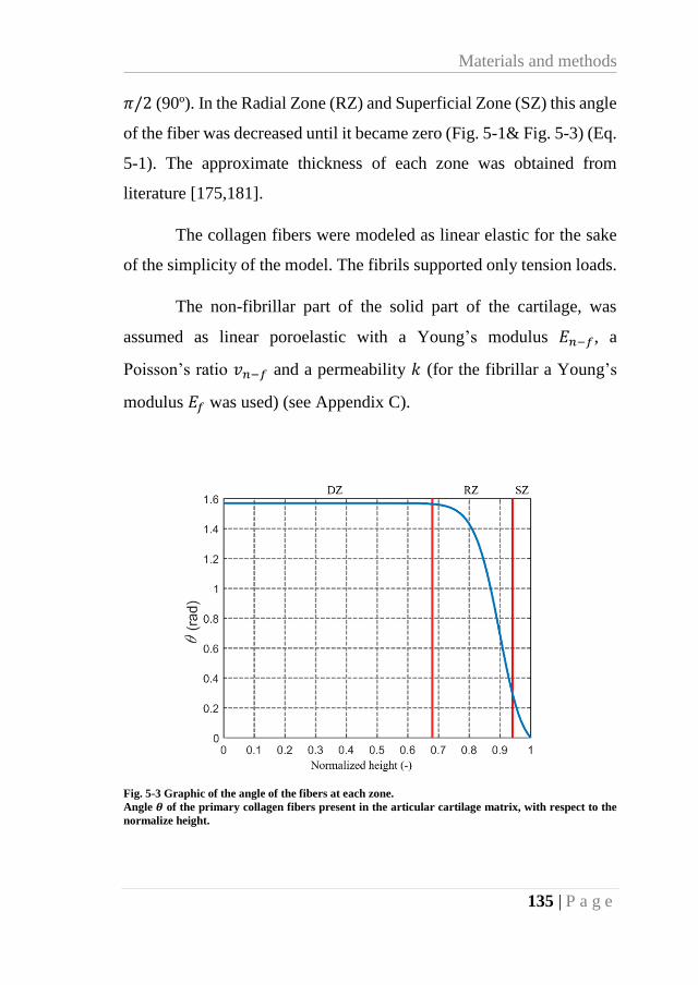
Materials and methods
135 | P a g e
𝜋/2 (90º). In the Radial Zone (RZ) and Superficial Zone (SZ) this angle
of the fiber was decreased until it became zero (Fig. 5-1& Fig. 5-3) (Eq.
5-1). The approximate thickness of each zone was obtained from
literature [175,181].
The collagen fibers were modeled as linear elastic for the sake
of the simplicity of the model. The fibrils supported only tension loads.
The non-fibrillar part of the solid part of the cartilage, was
assumed as linear poroelastic with a Young’s modulus 𝐸𝑛−𝑓, a
Poisson’s ratio 𝑣𝑛−𝑓 and a permeability 𝑘 (for the fibrillar a Young’s
modulus 𝐸𝑓 was used) (see Appendix C).
Fig. 5-3 Graphic of the angle of the fibers at each zone.
Angle 𝜽 of the primary collagen fibers present in the articular cartilage matrix, with respect to the
normalize height.
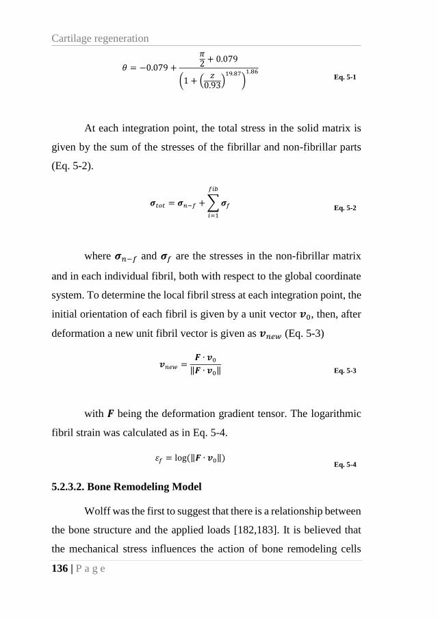
Cartilage regeneration
136 | P a g e
𝜃 = −0.079 +
𝜋2+ 0.079
(1 + (𝑧
0.93)19.87
)1.86
Eq. 5-1
At each integration point, the total stress in the solid matrix is
given by the sum of the stresses of the fibrillar and non-fibrillar parts
(Eq. 5-2).
𝝈𝑡𝑜𝑡 = 𝝈𝑛−𝑓 +∑𝝈𝑓
𝑓𝑖𝑏
𝑖=1
Eq. 5-2
where 𝝈𝑛−𝑓 and 𝝈𝑓 are the stresses in the non-fibrillar matrix
and in each individual fibril, both with respect to the global coordinate
system. To determine the local fibril stress at each integration point, the
initial orientation of each fibril is given by a unit vector 𝒗0, then, after
deformation a new unit fibril vector is given as 𝒗𝑛𝑒𝑤 (Eq. 5-3)
𝒗𝑛𝑒𝑤 =𝑭 ∙ 𝒗0‖𝑭 ∙ 𝒗0‖
Eq. 5-3
with 𝑭 being the deformation gradient tensor. The logarithmic
fibril strain was calculated as in Eq. 5-4.
휀𝑓 = log (‖𝑭 ∙ 𝒗0‖) Eq. 5-4
5.2.3.2. Bone Remodeling Model
Wolff was the first to suggest that there is a relationship between
the bone structure and the applied loads [182,183]. It is believed that
the mechanical stress influences the action of bone remodeling cells
Materials and methods
137 | P a g e
(osteoblasts and osteoclasts) through the osteocytes. It seems that
mechanosensitive osteocytes are capable of transducing changes in
mechanical stimuli into biochemical signals that regulate cellular
(osteoblasts and osteoclasts) responses [184]. Also, osteocytes may
detect matrix micro damage and signal for micro damage removal to
prevent accumulation of damage within the bone tissue [185,186].
Evidence shows that the formation of micro cracks through fatigue
damage may be the stimulus for bone remodeling, which begins with
bone resorption followed by bone formation [187]. Then, bones,
especially subchondral bone, can be adapted to loads on trajectories of
stress, through mineral apposition, i.e., more material is deposited in the
lines of high stress [188]. Furthermore, low stresses (low loads) are
commonly regarded as a reason for bone resorption since there is no
need to maintain the strength of the structure [189]. However, if the
bone stresses are so high (overloads) due to an abnormal load condition,
such as the implantation of a scaffold, the self-repair mechanism cannot
follow the increasing damage, and thus overload resorption will occur
[187]. For convenience, stress or strain can usually be considered as the
mechanical stimulus for bone remodeling [184,187].
Several computational models partly answer the mechano-
regulation of bone mass in response to strain and micro damage
[184,185,187,188,190–194]. One characteristic of most of those models
is the presence of a lazy zone (also known as equilibrium zone or
originally termed as dead zone), a range of mechanical stimulus (around
a value that the bone detects as normal) within which no change in bone
density is evident [195]. Therefore, net bone formation (or resorption)
Cartilage regeneration
138 | P a g e
is produced, if the mechanical stimulus is well over or below those
reference values.
Some studies have debated the likeliness of the presence of a
lazy zone [196], suggesting that bone remodeling is correlated with the
tissue loads following a linear relationship without a lazy zone.
Actually, the lazy zone seems more like a mathematical approximation
than a mechanobiological fact [195]. In fact, the inclusion of the lazy
zone has a serious drawback: the final bone density distribution depends
on the starting density, so the solution of the density distribution is not
unique nor guaranteed [195]. Hence, it can be said that the remodeling
response of the bone has a mechanobiological basis and governs the
behavior of the bone in every aspect.
It is believed that this mechanobiological response (bone
density redistribution or bone remodeling) is more complex than it
seems; a more complete model, as in Klika et al., [197], should include
variables like load frequency, hormonal response, cellular interactions
pathology, etc. [195]. Then, simplistic bone redistribution models
should be applied once the distribution of density is correctly
established, for example, to predict variations of bone density due to
changes in the normal activity [195]. In light of the aforementioned, and
for simplicity’s sake, we employed a basic bone remodeling model
which considers the response to strain, and the basal conditions as initial
conditions.
In our remodeling model, we considered the basal maximum
deformation (휀𝑚𝑎𝑥𝑏 ) of the bone tissues. Before the scaffold was
implanted, the basal maximum deformation was calculated as an
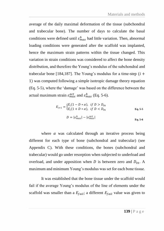
Materials and methods
139 | P a g e
average of the daily maximal deformation of the tissue (subchondral
and trabecular bone). The number of days to calculate the basal
conditions were defined until 휀𝑚𝑎𝑥𝑏 had little variation. Then, abnormal
loading conditions were generated after the scaffold was implanted,
hence the maximum strain patterns within the tissue changed. This
variation in strain conditions was considered to affect the bone density
distribution, and therefore the Young’s modulus of the subchondral and
trabecular bone [184,187]. The Young’s modulus for a time-step (𝑖 +
1) was computed following a simple isotropic damage theory equation
(Eq. 5-5), where the ‘damage’ was based on the difference between the
actual maximum strain 휀𝑚𝑎𝑥𝑎𝑐𝑡 and 휀𝑚𝑎𝑥
𝑏 (Eq. 5-6).
𝐸𝑖+1 = {𝐸𝑖(1 − 𝐷 ∗ 𝛼), 𝑖𝑓 𝐷 > 𝐷𝑡ℎ𝐸𝑖(1 + 𝐷 ∗ 𝛼), 𝑖𝑓 𝐷 < 𝐷𝑡ℎ
Eq. 5-5
𝐷 = |휀𝑚𝑎𝑥𝑏 | − |휀𝑚𝑎𝑥
𝑎𝑐𝑡 | Eq. 5-6
where 𝛼 was calculated through an iterative process being
different for each type of bone (subchondral and trabecular) (see
Appendix C). With these conditions, the bones (subchondral and
trabecular) would go under resorption when subjected to underload and
overload, and under apposition when 𝐷 is between zero and 𝐷𝑡ℎ. A
maximum and minimum Young’s modulus was set for each bone tissue.
It was established that the bone tissue under the scaffold would
fail if the average Young’s modulus of the line of elements under the
scaffold was smaller than a 𝐸𝑓𝑎𝑖𝑙; a different 𝐸𝑓𝑎𝑖𝑙 value was given to
Cartilage regeneration
140 | P a g e
each bone tissue. If the bone failed, the scaffold was able to move
downwards within the bone.
5.2.3.3.Potential vascularity factor
A hypothetic potential vascularity factor (PVF) was also
considered. This factor was assumed to diffuse from the bottom of the
domain, where it had a unitary concentration, towards the top of the
domain. This molecule had a low diffusion rate and determined if a
mesenchymal tissue might be vascularized or not.
5.2.3.4. Tissue regeneration model
In our model, we were dealing with the regeneration of two
types of tissue, cartilage and bone. The osteogenesis process might be
regulated by the mechanical environment, and it has been studied from
computational and experimental approaches. It is possible that the
sequential differentiation of precursor cells during bone healing is
highly influenced by the local mechanical stimuli [198]. Several
mechanoregulation algorithms have been proposed to analyze the
possible relationship between cell differentiation and mechanical
stimulation [7,199–201]. Also, these algorithms have been used to
simulate different aspects of tissue regeneration [202–210], and the
results have been compared to experimental outcomes. The tissue
regeneration algorithms regulated by deviatoric strain and FV were the
most accurate to predict healing as observed in vivo [211].
Cellular processes are another important aspect considered for
bone healing mechanoregulatory algorithms. Additionally, cell-
Materials and methods
141 | P a g e
phenotype specific actions influence on other cell mediated aspects of
bone healing, such as matrix production [204].
For bone regeneration, we proposed a model based Isaksson et
al., [204]. They developed a mechanistic model of tissue differentiation
which couples the cellular mechanisms to mechanical stimuli during
bone healing. They hypothesized that cells act as sensors of mechanical
stimuli. Therefore, cell proliferation, migration, differentiation or de-
differentiation, and production of cellular matrix are based on the
mechanical stimuli they are experiencing [204].
For the cartilage tissue, to our knowledge, there are not deep
computational models in literature to explain how this tissue is
regenerated. Hence, we consider three factors for its regeneration. First,
it was considered a positive relationship between cyclic hydrostatic
stress and cartilage growth [113]. Second, cartilage could only
regenerate in elements with mesenchymal tissue. Third, for cartilage to
regenerate it must have low concentration of PVF (hypothetic molecule
used as an indicator of the potential vascularity of the tissue).
Once there was any displacement of the scaffold due to failure
of the bone under it, the void on top of the scaffold was then filled with
mesenchymal tissue, which later would differentiate into other tissue
(bone or cartilage). This newly-formed tissue would initiate with a
concentration of mesenchymal cells.
If an element had mesenchymal tissue, only two paths could be
taken, either differentiates into cartilage, or follows the osteogenesis
model. For a mesenchymal element to differentiate into cartilage, the
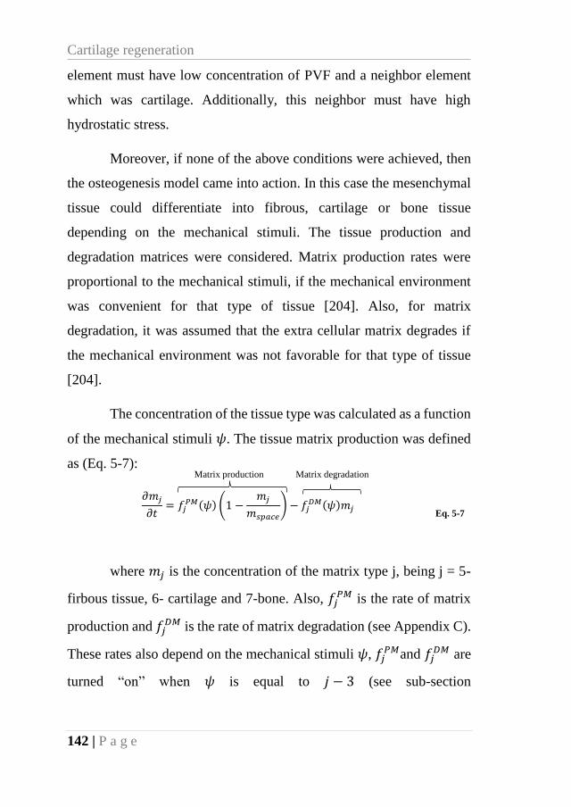
Cartilage regeneration
142 | P a g e
element must have low concentration of PVF and a neighbor element
which was cartilage. Additionally, this neighbor must have high
hydrostatic stress.
Moreover, if none of the above conditions were achieved, then
the osteogenesis model came into action. In this case the mesenchymal
tissue could differentiate into fibrous, cartilage or bone tissue
depending on the mechanical stimuli. The tissue production and
degradation matrices were considered. Matrix production rates were
proportional to the mechanical stimuli, if the mechanical environment
was convenient for that type of tissue [204]. Also, for matrix
degradation, it was assumed that the extra cellular matrix degrades if
the mechanical environment was not favorable for that type of tissue
[204].
The concentration of the tissue type was calculated as a function
of the mechanical stimuli 𝜓. The tissue matrix production was defined
as (Eq. 5-7):
𝜕𝑚𝑗
𝜕𝑡= 𝑓𝑗
𝑃𝑀(𝜓) (1 −𝑚𝑗
𝑚𝑠𝑝𝑎𝑐𝑒
) − 𝑓𝑗𝐷𝑀(𝜓)𝑚𝑗
Eq. 5-7
where 𝑚𝑗 is the concentration of the matrix type j, being j = 5-
firbous tissue, 6- cartilage and 7-bone. Also, 𝑓𝑗𝑃𝑀 is the rate of matrix
production and 𝑓𝑗𝐷𝑀 is the rate of matrix degradation (see Appendix C).
These rates also depend on the mechanical stimuli 𝜓, 𝑓𝑗𝑃𝑀and 𝑓𝑗
𝐷𝑀 are
turned “on” when 𝜓 is equal to 𝑗 − 3 (see sub-section
Matrix production Matrix degradation

Materials and methods
143 | P a g e
Mechanoregulation algorithm). 𝑚𝑠𝑝𝑎𝑐𝑒 is the space available in the
element for more tissue matrix and is calculated as follows [204]:
𝑚𝑠𝑝𝑎𝑐𝑒 = 𝑚𝑚𝑎𝑥 −∑𝑚𝑗
7
𝑗=5
Eq. 5-8
where 𝑚𝑚𝑎𝑥 is the maximal matrix concentration (see
Appendix C). The kind of tissue with higher matrix concentration
defines the new tissue for the element.
5.2.3.5. Mechanoregulation algorithm
As in previous studies [204], the combined effect of the
deviatoric shear strain (DSS) and FV was used to regulate cell and
tissue differentiation [199], which has shown to be versatile on
predicting bone healing [202,204,208,212]. Then, the DSS and the FV
were used to determine the value of 𝜓. For which, the mechanical
stimulation (MS) is calculated as follows:
𝑀𝑆 =𝐷𝑆𝑆
3.75+𝐹𝑉
3.0
Eq. 5-9
According to the mechanoregulation algorithm proposed by
Prendergast et al., 1997 [199]:
𝑀𝑆 > 3 𝜓 = 2 Fibroblast cells and fibrous tissue stimulation
3 ≥ 𝑀𝑆 > 1 𝜓 = 3 Chondrocyte cells and cartilage tissue stimulation
1 ≥ 𝑀𝑆 > 0.01 𝜓 = 4 Osteoblast cells and bone tissue stimulation
Cartilage regeneration
144 | P a g e
5.2.3.6. New Tissue
Some theories have been proposed on how the collagen fibers
within the cartilage get oriented in such unique way. It is hypothesized
that the particular collagen structure is consequence of the mechanical
conditions detected by the cartilage cells, which modify their ECM
accordingly [174]. Orientation of collagen fibers have been studied in
the aortic heart valve in which the collagen fibers (collagen type I) align
following the direction of the principal strain [213]. For cartilage,
whose fiber are collagen type II, it has been proposed that the fibers are
also oriented following the tensile strain direction, at least in the surface
[174].
In our model, the new tissue (mesenchymal) tissue has
differentiated into cartilage or any other (bone or fibrous tissue). If the
mesenchymal tissue differentiates into cartilage (new cartilage), fibrils
were placed within the new cartilage tissue oriented ±45º, as in Wilson
et al., [174]. Then, a collagen remodeling algorithm based on the one
proposed by Wilson et al., [174] was implemented. For each day (time-
step), the average direction of the maximal deformation was computed
and used to reorient the fibers direction. Conversely, if the
mesenchymal tissue differentiated into bone, it started with a small
Young’s modulus, which increased accordingly to the deformation of
the bone until the maximum limit was achieved.
5.2.4. GENERAL ALGORITHM
Fig. 5-4 shows a flowchart of the employed algorithm. The
model started, at 𝑛 = 1, with an initial mechanical analysis of the model
Materials and methods
145 | P a g e
where cyclic load was applied to the tissue for a number 𝑘𝑠𝑡𝑜𝑝 of steps.
From this analysis, stress, strain, and FV were calculated. These
calculations were averaged through each 𝑛 until little variation on the
average values was obtained (until 𝑛 = 𝑛𝑠𝑐𝑎𝑓𝑓); these values were used
as the basal values. At 𝑛 = 𝑛𝑠𝑐𝑎𝑓𝑓, a defect was introduced in the
articular cartilage and a scaffold was implanted within it. Thereafter,
for each time-step 𝑛, the mechanical analysis was conducted again and
stress, strain and FV average values are calculated, and tissue
remodeling, and regeneration were also conducted.
In the tissue remodeling and regeneration part of the algorithm
every element was analyzed. The path of the algorithm depended on the
type of tissue of the element 𝑗. If it was mesenchymal tissue, then it was
analyzed if it could differentiate into neo-cartilage or go through the
osteogenesis process. If the element was bone tissue, then it was
remodeled (resorption or apposition) according to its strain. If the
element had neo-cartilage tissue, then the collagen fibers within it
would reorient accordingly to the principal strain. Lastly, if the element
had new bone tissue, then its Young’s modulus would increase
depending on the strain of the element.
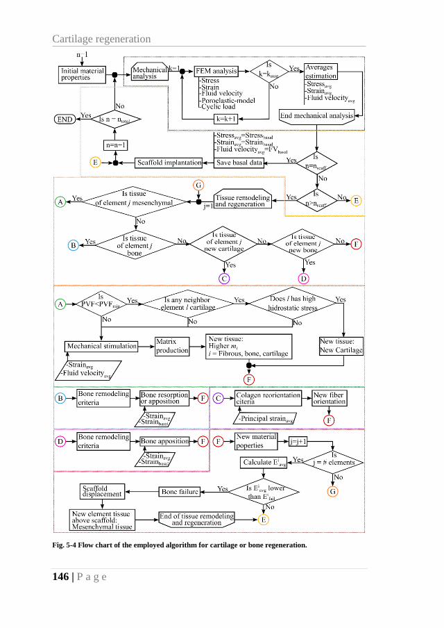
Cartilage regeneration
146 | P a g e
Fig. 5-4 Flow chart of the employed algorithm for cartilage or bone regeneration.
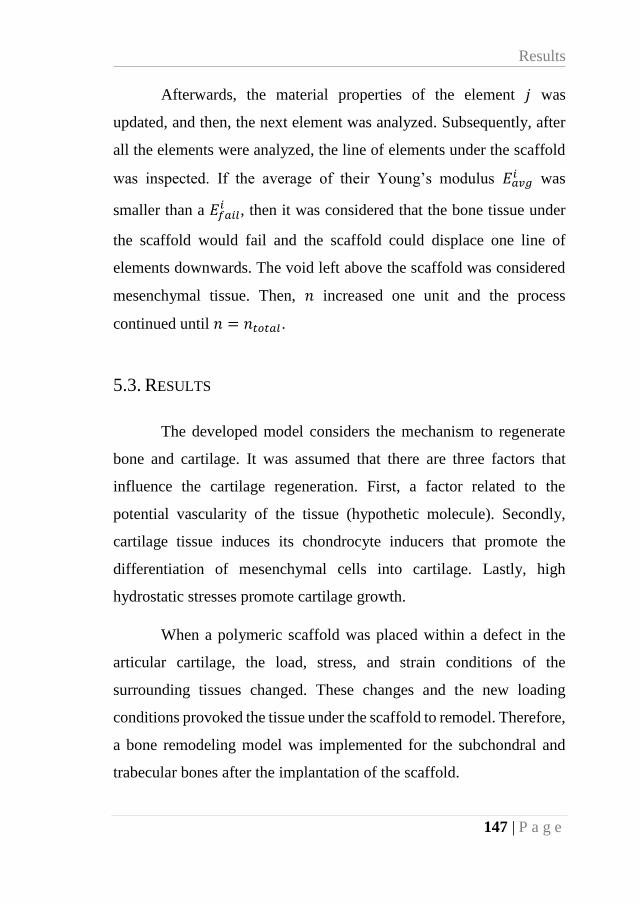
Results
147 | P a g e
Afterwards, the material properties of the element 𝑗 was
updated, and then, the next element was analyzed. Subsequently, after
all the elements were analyzed, the line of elements under the scaffold
was inspected. If the average of their Young’s modulus 𝐸𝑎𝑣𝑔𝑖 was
smaller than a 𝐸𝑓𝑎𝑖𝑙𝑖 , then it was considered that the bone tissue under
the scaffold would fail and the scaffold could displace one line of
elements downwards. The void left above the scaffold was considered
mesenchymal tissue. Then, 𝑛 increased one unit and the process
continued until 𝑛 = 𝑛𝑡𝑜𝑡𝑎𝑙 .
5.3. RESULTS
The developed model considers the mechanism to regenerate
bone and cartilage. It was assumed that there are three factors that
influence the cartilage regeneration. First, a factor related to the
potential vascularity of the tissue (hypothetic molecule). Secondly,
cartilage tissue induces its chondrocyte inducers that promote the
differentiation of mesenchymal cells into cartilage. Lastly, high
hydrostatic stresses promote cartilage growth.
When a polymeric scaffold was placed within a defect in the
articular cartilage, the load, stress, and strain conditions of the
surrounding tissues changed. These changes and the new loading
conditions provoked the tissue under the scaffold to remodel. Therefore,
a bone remodeling model was implemented for the subchondral and
trabecular bones after the implantation of the scaffold.
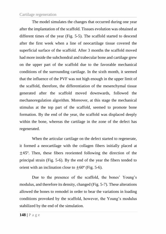
Cartilage regeneration
148 | P a g e
The model simulates the changes that occurred during one year
after the implantation of the scaffold. Tissues evolution was obtained at
different times of the year (Fig. 5-5). The scaffold started to descend
after the first week when a line of neocartilage tissue covered the
superficial surface of the scaffold. After 3 months the scaffold moved
had more inside the subchondral and trabecular bone and cartilage grew
on the upper part of the scaffold due to the favorable mechanical
conditions of the surrounding cartilage. In the sixth month, it seemed
that the influence of the PVF was not high enough in the upper limit of
the scaffold, therefore, the differentiation of the mesenchymal tissue
generated after the scaffold moved downwards, followed the
mechanoregulation algorithm. Moreover, at this stage the mechanical
stimulus at the top part of the scaffold, seemed to promote bone
formation. By the end of the year, the scaffold was displaced deeply
within the bone, whereas the cartilage in the zone of the defect has
regenerated.
When the articular cartilage on the defect started to regenerate,
it formed a neocartilage with the collagen fibers initially placed at
±45º. Then, these fibers reoriented following the direction of the
principal strain (Fig. 5-6). By the end of the year the fibers tended to
orient with an inclination close to ±60º (Fig. 5-6).
Due to the presence of the scaffold, the bones’ Young’s
modulus, and therefore its density, changed (Fig. 5-7). These alterations
allowed the bones to remodel in order to bear the variations in loading
conditions provoked by the scaffold, however, the Young’s modulus
stabilized by the end of the simulation.
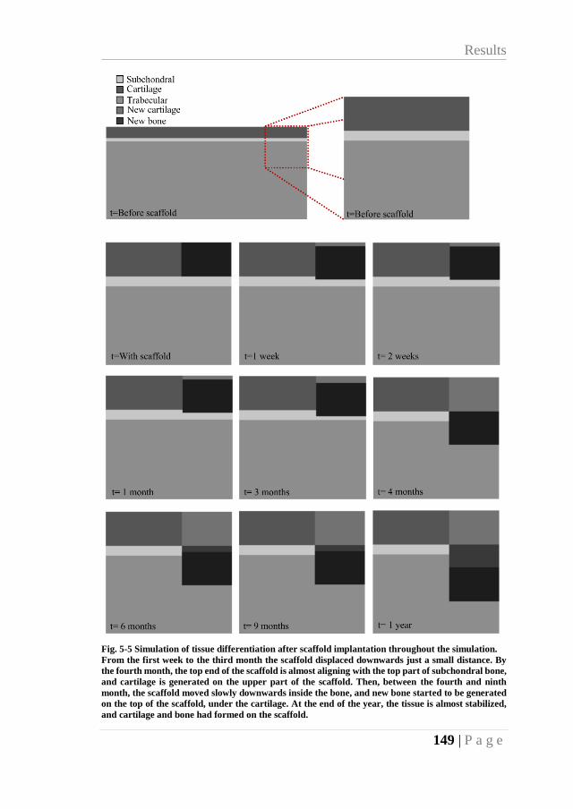
Results
149 | P a g e
Fig. 5-5 Simulation of tissue differentiation after scaffold implantation throughout the simulation.
From the first week to the third month the scaffold displaced downwards just a small distance. By
the fourth month, the top end of the scaffold is almost aligning with the top part of subchondral bone,
and cartilage is generated on the upper part of the scaffold. Then, between the fourth and ninth
month, the scaffold moved slowly downwards inside the bone, and new bone started to be generated
on the top of the scaffold, under the cartilage. At the end of the year, the tissue is almost stabilized,
and cartilage and bone had formed on the scaffold.
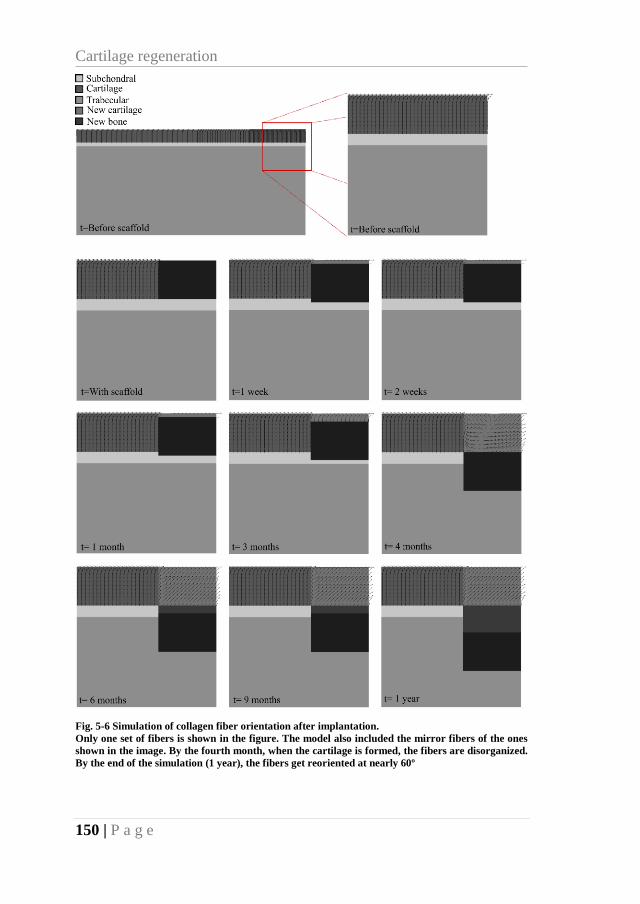
Cartilage regeneration
150 | P a g e
Fig. 5-6 Simulation of collagen fiber orientation after implantation.
Only one set of fibers is shown in the figure. The model also included the mirror fibers of the ones
shown in the image. By the fourth month, when the cartilage is formed, the fibers are disorganized.
By the end of the simulation (1 year), the fibers get reoriented at nearly 60º
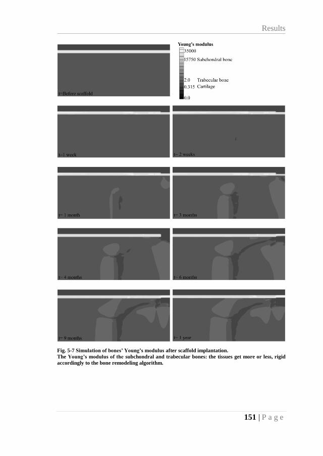
Results
151 | P a g e
Fig. 5-7 Simulation of bones’ Young’s modulus after scaffold implantation.
The Young’s modulus of the subchondral and trabecular bones: the tissues get more or less, rigid
accordingly to the bone remodeling algorithm.
Cartilage regeneration
152 | P a g e
5.4. DISCUSSION
We developed a model to explain some of the processes that
influence cartilage regeneration when implanting a polymeric scaffold
in the site of an articular cartilage the defect. The subchondral bone,
trabecular bone, cartilage and scaffold were considered in the model as
poroelastic materials. The cartilage’s collagen fibers were modeled as a
linear elastic, tension only, material.
The model considers the basal conditions of the system, that
means, the stress and strain conditions when the scaffold is not yet
implanted. These data were then compared to the ones obtained when
the scaffold is implanted. The differences between both states, allowed
to determine the remodeling behavior of the bones, which helped to
decide whether the bone should either reabsorb or densify by apposition
at specific zones. This meant that a reduction of bones’ strain (low
loads) would translate into bone resorption [189]; a small increase of
strain (‘medium’ loads) translated to bone apposition (bone resorption
followed by a quick bone formation) [187]; and finally, a high increase
of bones’ strain (overload) was also assumed as bone resorption [187].
This simulated the normal behavior of a bone tissue that goes under a
remodeling process [187,189].
Bone resorption and appositions processes, bone remodeling,
was modeled as a change in the Young’s modulus of the bone. An
increase and a reduction of the Young’s modulus was assumed when
the apposition or resorption processes took place, respectively (Fig.
5-7). Trabecular bone had to remodel in order to bare the abnormal load
Discussion
153 | P a g e
brought by the scaffold (Fig. 5-7). Moreover, the Young’s modulus of
the trabecular bone increases at the zone under the scaffold once is
implanted; but decreases, due to overload, on line right under the
scaffold (Fig. 5-7). However, by the end of the simulation time (a year),
the trabecular bone’s Young’s modulus had the tendency to return to
basal conditions, which can be considered as if the system is stabilizing
(Fig. 5-7).
The scaffold was displaced inside the bone if the Young’s
modulus of the bone under the scaffold was small. This displacement
left a void on the top of the scaffold, which was assumed to be filled
with mesenchymal tissue. This mesenchymal tissue, as soon as it was
generated, had two options, either differentiate into cartilage or follow
an osteogenesis process algorithm; within which it could differentiate
into fibrous tissue, cartilage or bone, depending on the mechanical
stimuli. To differentiate into cartilage, the mesenchymal tissue must
fulfill three conditions: First, the concentration of PVF had to be low
enough so that differentiation into tissue with low vascularity were
promoted. Secondly, the tissue that surrounds the mesenchymal one had
to be cartilage, this way, the influence of the chondro-inductive
molecules that might diffuse from the cartilage tissue is simulated.
Third and lastly, it was assumed that cartilage growth is induced under
high hydrostatic conditions, therefore, not only the surrounding tissue
needed to be cartilage, but it also needed to bear high hydrostatic loads.
In the results, cartilage started forming on the top part of the scaffold
until the fourth and sixth month, where the concentration of the PVF
was high enough to avoid the formation of cartilage (Fig. 5-5).
Cartilage regeneration
154 | P a g e
Initially, the new formed cartilage had collagen fibers in a
‘disorganized’ way, later it aligned following the direction of the
principal strain. After the simulation time, the final direction of the
fibers was about 60º. In this model, the new fibers did not align entirely
as the fibers of a native articular cartilage (Fig. 5-6); factors that we did
not consider could be influencing the reorientation of the new collagen
fibers, which should be addressed in future models.
If the conditions for a mesenchymal tissue to differentiate into
cartilage were not fulfilled, the osteogenesis process algorithm
happened. We calculated a mechanical stimulus for the osteogenesis
algorithm, and it defined whether the mesenchymal tissue should
differentiate into cartilage, bone, or fibrous tissue. In our model, the
calculated mechanical stimulus was ideal to stimulate the mesenchymal
tissue to differentiate only into bone (Fig. 5-5).
A previous experiment from our group implanted polymeric
scaffold as treatment to repair a chondral defect [4]. In that study, a full-
depth chondral defect was made in the knee joint in a rabbit
experimental model, where a biostable, poly (ethyl acrylate-co-
hydroxyethyl acrylate) copolymer, porous scaffold was implanted. We
studied the evolution of the cartilage repair process through histological
techniques. Histological images for 1 and 2 weeks, and for 1, 3, and 12
months after implantation [4]. At early stages (first months), we
observed a thin layer of tissue covering the scaffold surface (Fig. 5-8).
In the results of our model, it can also be observed that for the first
months, there was also a thin layer of new cartilage tissue that was
formed on the upper part of the scaffold, which agrees with our findings
Discussion
155 | P a g e
[4] (Fig. 5-8). At 3 months, the scaffold was completely covered by a
thicker layer of new cartilage [4]. In our computational model, the
results at three months also agree with the ones observed in the
experiment (Fig. 5-8). A year after the implantation of the scaffold, the
cartilage in the experimental model was completely repaired, and the
scaffold was displaced towards the inside of the bone; in our
computational model it is also observed that the scaffold was displaced
inside the bone, whereas the defect in the articular cartilage was already
covered (Fig. 5-8).
It should be considered that our model assumed some
simplifications for computational savings. For example, the cartilage
was modeled as poroelastic, when it is well known that the cartilage is
composed by a more complex material. Moreover, the fibers within the
cartilage were modeled as linear elastic but their real behavior might
imply more variables and a more complex model. Also, the model
employs a 2D geometry, and the fibers of the cartilage were only
modeled in this 2D-plane, but in reality, they align in a 3D direction.
However, despite all the simplifications made, when comparing the
results of our computational model, with those of the experimental
model developed by Sancho-Tello et al., [4], it can be seen that our
model is able to predict various results: the tissue evolution of the
cartilage repair process phenomenon, the time of repairing, and the final
results of the treatment. Our computational model could be useful when
a comparison on the effect of using different scaffold materials is
wanted, or when different loading conditions or tissue degeneration is
required and compared with an idealized treatment condition. We

Cartilage regeneration
156 | P a g e
conclude that the proposed model is promising and might be helpful
when planning treatments for articular cartilage regeneration.
Moreover, this model might be useful as an analysis tool prior
experimental in vivo studies, allowing to discard approaches that might
not bring good results which at the end translates to a reduction on the
need of animal use.
Fig. 5-8 Comparison of our results with the histological findings of a previous experimental study.
At the left, tissue evolution obtained with our simulation model where the zone near the scaffold is
zoomed-in and mirrored. At the right the histological images obtained by the experimental model
developed in Sancho-Tello et al., [4]. Histological images modified from [4].
157 | P a g e
Chapter 6. GENERAL CONCLUSIONS
AND RECOMMENDATIONS
6.1. GENERAL CONCLUSIONS
The principal aim of this thesis was to computationally model
the mechanical and biochemical aspects involved in the development of
synovial joints. Therefore, this work portrays two models to explain the
joint development from the interzone onset to morphogenesis (Joint
Onset and Joint Morphogenesis). Additionally, it was also proposed an
extra computational study, related to joint development, in which three
different theories for patella development were explored through
computational models (Patella Onset). Moreover, another model was
developed to explain some phenomena related to the articular cartilage
regeneration (Cartilage regeneration).
All the computational models developed in this study employed
theories about tissue behavior under mechanical and biochemical
stimuli. The obtained results, when compared to experimental works
found in the literature, showed promising outcomes. Hence the
procedures and considerations taken for each proposed computational
model are not far from what is really happening on the analyzed
biological phenomena.
From the outcomes of this work we can say that the
interphalangeal joint development can be explained through the
General conclusions and recommendations
158 | P a g e
interaction of only six (generic) molecules, each of which played an
important role in the joint onset These proposed generic molecules can
be related to real molecules that have been shown that might influence
joint development. It should be pointed out that the human body is a
redundant system (there are groups of molecules which might do the
same task in case the principal molecule fails), which is the reason why
we did not tie to specific molecules. Moreover, it was found a good
correlation when the results of the joint onset model were compared to
the histological observations found in literature, which is an indicator
that the proposed interaction of the molecules is a reliable
approximation of what is happening in the joint onset process.
Once the joint begins its development, after the interzone
appearance and the cavitation processes, comes the morphogenesis: a
stage in which the joint gets its final shape. In the computational model
that we proposed for this stage, we believed that both, mechanical loads
and molecular factors, have an influence on how the shape of the joint
evolves. A remarkable similitude was found when the obtained results
were compared to anatomical observations of an interphalangeal joint.
Moreover, we obtained better results than those of previous
computational model describe by other authors, in which only the
mechanical load was considered. Then, the outcomes of our
computational model suggest that, in fact, both stimuli (mechanical and
biochemical) are necessary for the joint morphogenesis process.
Within some synovial joints, there are some small bones called
sesamoid bones, the largest being the patella. However, there is a lot of
debate regarding why and how these bones develop. Some theories have
General conclusions
159 | P a g e
been proposed to explain the formation and function of the patella, but
still there is not a unified theory that clarifies the development of these
bones. In order to explore this issue, we developed a computational
model for each one of the theories found in the literature, as a tool to
evaluate their likelihood. Three theories were evaluated, two of them
with a mechanical approach and the other with a biochemical one. With
our computational models we were able to predict the patella onset with
all three theories, being the “biochemical theory” the one that showed
better results, i.e., a better resemblance with the anatomical and
histological observations. However, since there are studies that have
found that mechanical loads influence joint development (studies where
the limb was immobilized and the patella developed but smaller than
control), we propose that the molecular interaction triggers the patella
onset and that mechanical loads are necessary for the patella growth and
maintenance.
Once the synovial joint and all the related structures have
developed, there are some pathologies that might affect the internal
structures of the joint, compromising its functionality. It was of our
interest to evaluate a treatment employed for one of these pathologies,
thus we focused on a novel therapy used to repair injuries in the articular
cartilage. So, we developed a computational model in which we intend
to characterize aspects that might influence cartilage regeneration when
a polymeric implant is used. We based the model on experimental
outcomes of previous works, and we obtained coherent results. In our
model, we observed that not only the cartilage has to adapt during the
regeneration process but also the surrounding tissue, e.g., subchondral
General conclusions and recommendations
160 | P a g e
and trabecular bone. The developed computational model could be
helpful to compare different scaffold materials and load conditions and
evaluate which approach results in a better outcome.
With the developed computational models of this thesis we were
able to the evaluate mechanical and biochemical conditions of some
biological phenomena, that would be difficult to test through
experimental approaches. This work explored several aspects of the
joints (synovial) from its development to its mature state. We hope that
these models become useful for medical and biological researches,
helping in the design of prevention and therapy strategies for joint
related pathologies.
6.2. RECOMMENDATIONS
• The developed computational models could be improved by
employing more complex material models for the tissues. However, it
should be considered the computational cost that this would imply.
• For future work, it is suggested to apply the methodologies
proposed for interphalangeal joint onset and morphogenesis to other
joints, such as the hip joint, to evaluate the happenings of
developmental pathologies like the DDH. Moreover, our model can be
extended by adding the effect of load prior to the cavitation process
(since it is believed that loading starts affecting the development of
large joints prior to the cavitation process).
• For the patella development, it is suggested that a general model
should be developed, in which the biochemical theory is combined with
Recommendations
161 | P a g e
the mechanical one. It is advised that the biochemical theory triggers
the formation of the patella, and once the tendon is fully developed, the
mechanical loading shapes and maintain the patella.
• Cartilage regeneration model can be widened by considering the
effect of other tissues, scaffold structures, types of biomaterials and
molecules that could influence the cartilage regeneration.
• Although the developed models were proposed in 2D and show
good results in the task of explaining the biological processes studied,
it must be evaluated if it is worthwhile to translate some of these models
into a 3D environment.

163 | P a g e
SUMMARY
Joints connect the skeletal components of the body and enable
a relative movement between them. Among the different kind of joints,
the synovial ones offer the widest range of motion between the bones.
Most synovial joints are in the appendicular skeleton (limbs).
Depending on the joint, they can have different internal structures.
However, they all have four common features: the enclosed articular
capsule containing synovial fluid (lubricant); the articulating
cartilaginous surfaces at each end of the bone, which slide against each
other; the synovial membrane, which covers the inner surface of the
capsule; and the ligaments, tendon and muscles, which provide stability
and mobility to the joint.
How is this kind of joint formed? Studies have shown that onset
and development of synovial joints are regulated by different genetic,
biochemical and mechanical factors. The synovial joints development
is a multipart process that starts in the fetal stages of prenatal
development. Around five weeks of development, limb buds start
growing and become noticeable. At the beginning, these limb buds have
an uninterrupted mass of mesenchymal cells within its core. This bulk
of cells is known as skeletal blastema and it is covered by a layer of
ectoderm. Then, most of these blastemal cells differentiate into
chondrocytes, although, some of them remain undifferentiated at the
interzone, where the future joint will form. The separation of the joint
occurs during the cavitation process, in which interzone cells are likely
Summary
164 | P a g e
suffer apoptosis, leaving a space between the chondrocyte bone
rudiments.
After the joint cleavage (cavitation), joint morphogenesis occurs
as cells proliferate on both sides of the joint, allowing the head of the
bones to take their final shape. Studies have shown that the shaping of
the joints is influenced by movements and muscle contractions that are
present during limb development, although local and systemic
biochemical factors could also have some effects. If there are abnormal
conditions during fetal development, joints can develop incomplete or
abnormal, or even they might not develop at all.
Once the embryonic period has finished, the synovial joint and
its internal structures (like the articular cartilage, ligaments and
synovial capsule) are completely developed. Moreover, POC and SOC
of the bone appear. These structures help the bone grow and ossify until
the adulthood is reached.
However, once the synovial joints are formed, they might suffer
several pathologies that impair their movement and probably affect the
lifestyle of the individual who is suffering from it. These pathologies,
such as the OA, which is a degenerative joint disease, can occur due to
repeated trauma, aging, surgery, obesity, hormonal disorders, injuries
on the joint surfaces and overloading due to abnormal shape of the joint,
among others.
In the OA, the wear and degeneration of the articular cartilage
can eventually cause the loss of a portion of it. This condition is
worsened by the poor ability of the cartilage to regenerate itself. The
Summary
165 | P a g e
worn cartilage is generally replaced by an unsuitable tissue, fibrous
cartilage. This new tissue produces an uneven articular surface that
causes friction, which can trigger joint pain and stiffness, aggravating
the pathology.
Several treatments have been proposed to repair the articular
cartilage and they range from symptomatic to more invasive ones, being
the last resort a total replacement of the affected joint or joint
arthrodesis treatments, i.e. fusion of all or some of the bones that are
part of the synovial joint. Of course, it is preferable to preserve the
original structure and function of the joint rather than a joint
replacement or an arthrodesis, especially in the case of young patients.
Tissue engineering has been trying to find definitive treatments
for degenerative pathologies of articular cartilage by proposing less
invasive approaches to these injuries. In the last two decades, the use of
scaffolds has been proposed as an alternative treatment to the
osteochondral graft. The scaffolds allow a rapid filling of the joint
defects and provide cells a substrate for anchoring. The use of scaffolds
in tissue engineering involves three main components: scaffolds’
materials, cell differentiation factors and cellular sources. In addition,
scaffolds without cellular sources have also been used showing
excellent results, avoiding the risks associated with cell manipulation
(e.g., contamination of bacteria and phenotype loss during handling), as
well as reducing costs.
It is vital to understand the processes through which the joint
tissue goes from its development to its maturity stage in order to
Summary
166 | P a g e
develop new direct and effective therapeutic strategies for pathologies
related to the joints. However, to achieve it entirely through
experimental analyses could lead to a great consumption of resources
and time. Therefore, computational models appear as a convenient tool
to complement the study of the joint processes. Computational models
provide a quantitative and qualitative evaluation of mechanical and
biological interactions while feeding on clinical or experimental
observations. Therefore, computational models contribute to these
studies since they evaluate difficult-to-reach aspects for experimental
models.
This thesis studies, through computational models, the
controlled biochemical interaction that occurs at the onset of the
interzone and the cavitation process during the synovial joint
development. In the case of the morphogenesis process, besides the
biochemical interaction, the possible effect of the mechanical load that
could be present during the shaping process of the epiphyses of the
bones is also considered.
As part of the development, we also analyzed, computationally,
different theories that have been proposed to explain the existence of
the sesamoid bones; bones which are superficially embedded within
tendons and are usually around joints. This study is focused on the
patella (kneecap), which is the largest, most recognized and studied
sesamoid bone in the human body.
Moreover, we also analyzed through a computational model the
processes that occur when a defect in the articular cartilage is treated
with the implantation of a polymeric scaffold. This may be useful to
Summary
167 | P a g e
compare different scaffold materials, shapes, and conditions of the
scaffold that could influence the outcome of the treatment.
To summarize, the objectives of this thesis are:
Principal aim:
To model, computationally, the mechanical and biological aspects that
occur during the development of synovial joints.
Specific aims:
- To formulate the mathematical description of the
mechanobiological phenomena that govern the development of
the synovial joints.
- To computationally evaluate the behavior of the model during
the interzone onset of synovial joints.
- To computationally evaluate the behavior of the model during
the cavitation process and morphogenesis of synovial joints.
1- Joint Onset
1.1.Methodology for the joint onset model
A computational model was developed based on two generic
molecular actions and two molecular self-regulatory loops, expressed
as reaction-diffusion equations. The aim was to predict the molecular
patterns associated with the joint formation process. The model was
solved in a finite elements’ framework. Mathematical equations
predicted patterns that represent molecular mechanisms that model the
structures and shapes during joint development, such as interzone
formation, cavitation, and condylar shape of the bone ends.
Summary
168 | P a g e
Reaction-diffusion equations and the formation of Turing
patterns were used to simulate the location of joint cleavage, the number
of joints formed, the sides of the joints that would form the epiphyses,
and the initial condylar shape of the joint.
Based on the molecules that have been reported in the literature
to have a role on joint development, six generic molecular factors
involved in joint onset were modeled. Note that each factor may
represent multiple molecules achieving the same action. The process in
the model was organized in two stages. The first one marked the
interzone onset, factor (G), which was located at the cleavage position
while its antagonist, and was also considered a factor (N), located
everywhere else. Factor (G), which was related to GDF-5, prevented
the differentiation of the mesenchymal tissue into cartilage, whereas
factor (N) was associated to the BMP antagonist Noggin. In the second
stage, the zones that differentiate into cartilage secreted Ihh, factor (I),
and PTHrP, factor (P), both establishing a regulatory loop that governs
cell proliferation and hypertrophy. Factor (I) regulated chondrocyte
proliferation, maturation, and hypertrophy, whereas factor (P) inhibited
chondrocyte hypertrophy.
Meanwhile, the domain kept growing and two other factors, (H)
and (W), regulated the joint separation and related structures. (H)
controls the differential amount of tissue growth from proximal to
distal. Mathematically, there was a gradient in (H) that affected the
growth rate by promoting the longitudinal growth of the limb and bones
anlagen. (W), expressed in the interzone, induced cell death and
allowed the generation of a joint space. Factors (H) and (W) leaded to
Summary
169 | P a g e
separation of the rudiments and was also observed in parts of the fibrous
capsule in later stages of development.
The finite element model included a PDE integrated with a CA-
like system (PDE+CA-like). The PDE part described the molecular
diffusion and established the biochemical concentrations, which enable
the CA-like part to determine whether the tissue differentiated or not.
Each element started with a tissue state (mesenchymal, pre-
cartilaginous, cartilaginous, or interzone) and the CA-like system
allowed the element to differentiate from one tissue state to another.
This process loops until the stop criteria is reached (joint cleavage and
its initial shaping).
Four different cases were explored. In Case I, the conditions for
the development of an interphalangeal joint were established. The
following three cases were modifications of the first one. In Case II and
Case III, the effect of changing the dimensions of the initial domain in
the joint development was tested. In Case IV, we analyzed how the
growth rates of the domain modified the outcome. Besides, a parallel
experimental procedure was replicated, in which GDF-5 beads were
implanted in the side and tip of a developing chick autopod.
1.2. Results and discussion from the joint onset model
In Case I, the comparison of the obtained results for factor (G)
with expression of GDF-5 in experimental studies demonstrated similar
distributions. Additionally, the loop (I-P) results in a distribution where
(P) was near the distal ends and (I) was at the proximal ends of the
rudiment, as seen for Ihh and PTHrP in the literature.
Summary
170 | P a g e
The factor (W) established the formation of the articular
cartilage in each articular surface and was consistent with the
distribution of Wnt in the literature. The shape of the joint was
comparable with the histologic findings: both sides of the joint have
articular cartilage, but on one side there is an epiphysis-like structure.
This leaded to the formation of a larger epiphysis-like at the distal end
and another not so wide at the proximal end. From this point on, the
morphology of the joint is likely influenced by mechanical conditions.
The obtained results suggest that the size of the initial domain
during development may have an influence on the number of joints
formed. In the simulation, one and three joints were acquired when the
length/width ratio was established in 3 (Case I) and 5 (Case II),
respectively. It is known that Turing patterns depend on the domain
ratio, therefore the number of joints must depend on the initial
geometry. Nevertheless, the literature shows that one joint is formed at
a time and that is why, we propose that a joint might formed each time
the distal anlage within a limb bud reach a ratio of approximately 3.
In Case III (faster growth velocity), a single joint was obtained
with two growing regions located at both ends of the rudiments with
high concentrations of (I). In Case IV, the goal was to simulate the onset
of a joint located between a large bone and a shorter one (e.g. between
a metatarsal or a metacarpal and a phalanx). Therefore, the length/width
ratio of its initial domain was set to 2.5.
Case V and Case VI simulate the experimental study performed
by Merino et al., which analyzed the effects of placing GDF-5 beads in
the developing autopod of embryonic chicks, specifically at the tip of
Summary
171 | P a g e
the digits. Comparing the results from Case V and Case VI with those
reported in Merino et al., three similarities were found: a very similar
morphology was achieved, the resulting rudiment was curved when the
molecule is implanted on one side of the mesenchymal condensation,
and a bulb was formed when (G) was implanted at the tip of the mold.
These effects might be explained since high concentration of (G) which,
after the cavitation process, implied high concentration of (W)
encouraging the differentiation of the tissue into articular cartilage. This
abnormal location of articular cartilage impacts on the Turing pattern
between (I) and (P), hence abnormal growth of the tissue was obtained.
In this thesis, a simplified model to study the development of
joints was proposed. A good agreement was found between the results
obtained with the simulation model and those reported in the literature
for experimental works where histological analyses were performed.
Although multiple molecules often influence the same biological
process, it was shown, by modeling generic molecules, how the pattern
formation of simple patterns between enzyme-substrate molecules
predicts many events present in joint formation. The model shows a
good response with interphalangeal and metacarpal/metatarsal-
phalangeal joints. The results obtained in the study of this chapter will
be useful for researchers focused on pathologies associated with
embryo and joints development. Furthermore, this model could provide
new insights and guidelines of experimentation and, of course, new
mathematical and computational models of the following phases of
joint development.
Summary
172 | P a g e
2- Joint Morphogenesis
2.1. Methodology for the joint morphogenesis model
After the interzone onset and cavitation process, takes place the
last step of joint development, its morphogenesis. Experimental and
computational studies have shown that there is a relationship between
mechanical stress and skeletal morphogenesis. From a computational
perspective, two models have been developed to evaluate the
relationship between joint morphogenesis and mechanical stresses.
Heegaard et al. and Giorgi et al., both computational studies, used the
hydrostatic stress distribution for describing the growth and joint
morphogenesis. Although those studies obtained relevant results on the
morphogenesis process, the final shapes of the two opposing rudiments
do not match to with the actual interphalangeal morphology, indicating
that biochemical interactions during bone morphogenesis might be
necessary to achieve congruent joint shapes. Nevertheless, to date, there
is still no experimental or computational model able to accurately
explain how a synovial joint is shaped. Thus, the aim of this section is
to develop a computational model that might bring us closer to
understanding the process of joint morphogenesis.
A 2D finite element model of the interphalangeal joint that
includes the synovial capsule was developed. This model considered
the biochemical and mechanical effects on the joint morphogenesis,
from the cavitation stage to the appearance of POC and SOC.
The model initiated with the last obtained geometry of the
previous section model. This geometry was the first reference
geometry. Then, the distal bone anlage of the reference geometry was
Summary
173 | P a g e
rotated to simulate the movement of the finger; only four steps of the
movement were evaluated: 90º, 60º, 30º and 0º. The calculations were
made on each position and then translated into the reference geometry
(0º) and averaged in each element. Then, the average cartilage growth
and ossification parameters were computed and used to update the
reference geometry. Afterwards, the distal phalanx was rotated again to
the positions analyzed. This process continued until the shape of the
joint agreed with the shape of an interphalangeal joint.
Regarding the mechanical part of the model, an axial
displacement of 1𝜇𝑚 was applied to the upper boundary of the distal
phalanx. The proximal phalanx was fixed at its bottom on the central
node so that the other nodes of the lower end could move in the lateral
direction. The cartilage of the anlagen bones was assumed to be almost
incompressible.
The effect of the PTHrP and Ihh molecules was also considered.
Ihh controls chondrocyte proliferation, maturation, and hypertrophy,
whereas PTHrP inhibits chondrocyte hypertrophy. Additionally, a
remaining part of the molecule Wnt was considered because of its
action on the morphogenesis process. The initial distribution of these
molecules was taken from the last step of the simulation performed in
the previous section.
For tissue growth, it was assumed that the tissue response to
mechanical stimuli had a positive relationship between cartilage growth
and cyclic hydrostatic stress, and it was inhibited by octahedral shear
stress. Additionally, it was considered that high concentrations of
Summary
174 | P a g e
PTHrP and Wnt promoted chondrocyte proliferation and, consequently,
cartilage growth.
For the bone ossification, the OI was used to predict the
appearance of the POC and SOC within the anlagen. It was considered
that the cartilage in the diaphysis ossified under high OI and low PTHrP
and Wnt, whereas for the SOC appearance, only the OI is considered.
2.2. Results and discussion from the joint morphogenesis
model
Four different positions of the interphalangeal joint were
analyzed. The same weight was given to each position, since there are
no reports in the literature about how the fingers of the fetus move
during the morphogenesis stage. The obtained final shapes of the bones’
diaphysis were coherent with those seen in literature.
The appearances of SOC and POC were also simulated. SOC
emerges in the top head of the proximal phalanx and in the lower head
of the distal phalanx. In the proximal phalanx, it is formed as a circular
shaped structure. In the distal anlage, the SOC took an elliptical shape,
most likely due to the way in which the convex surface distributed the
octahedral shear stress and hydrostatic stress (used to calculate the OI).
In places of low concentrations of PTHrP and high
concentrations of Ihh, the chondrocytes became hypertrophic and the
tissue eventually ossified forming the POC. The model showed how the
OI predicts areas of high ossification on the diaphysis, and how the
PTHrP and hydrostatic stresses helped with the cartilage growth and
maintenance. The obtained results are comparable with those from
Summary
175 | P a g e
former studies where only the endochondral ossification and OI
distribution was analyzed.
The obtained joint shape agrees remarkably with those observed
in x-rays. Therefore, this work sheds some light on how the mechanical
environment, combined with biochemical factors, influences the
morphogenesis of a synovial joint. It is worth mentioning that dynamic
hydrostatic stress, since it promotes cartilage growth, is key to joint
morphogenesis. However, for a joint to achieve complex shapes, it is
necessary to include cell/tissue responses to biochemical and
mechanical stimuli.
The presented model offers an excellent approximation of what
is happening during joint development and morphogenesis and provides
a new understanding of these processes which, eventually, may lead to
the development of new treatments for developmental pathologies, or
even prevent malformations of the fetus.
3- Patella Onset
There is still a lack of understanding about the development of
the patella. The most accepted theory is that it develops inside the
tendon in response to mechanical stimuli. While the tendon is
immature, a zone of the tendon is subjected to high hydrostatic stress
and low tensile strain. This leads to the differentiation of the fibrous
tissue precursor into cartilage and then to the ossification of the
cartilage to form the patella.
Currently, according to the best of our knowledge, there is no
accepted nor unified mechanism in the literature that explains the
Summary
176 | P a g e
formation of sesamoid bones. The aim of this part of the document was
to evaluate, separately, the outcome of three conceptual computational
models for the development of the kneecap. The first model considered
the biochemical aspects present at the onset of the quadriceps tendon
and the patella. The second model examined the cellular behavior under
the mechanical stimuli present during the formation of this sesamoid
bone. And the third model optimized the mechanical environment of
the tissues through topological optimization (TO) based on the
minimizing the strain energy.
3.1. Biochemical theory
This biochemical theory was first proposed by Eyal et al.
According to this theory, the patella develops as a bone eminence
attached to the distal femur end, where new sox9-positive chondrogenic
cells attach to the mentioned femoral end. This new aggregation of
chondrogenic cells is separated from the preexisting cartilage because
of the effect of a remaining joint inducer on the articular surface of the
femur.
The model started with the initial conditions given by the
concentrations of the molecules and a domain of Scx-cells. Then, TGF-
β and BMP diffused from muscle and bone and, consequently, the Scx-
cells were attracted towards high concentrations of TGF-β. Once the
muscle detected the presence of Scx-cells, it expressed FGF. The
differentiation process involved the Scx-cells and the concentrations of
FGF and BMP. If there was enough concentration of Scx-cells and
BMP, the cells differentiated into chondrocytes, whereas if there was
enough concentration of Scx-cells and FGF, the cells differentiated into
Summary
177 | P a g e
tenocytes (tendon tissue). At the same time, the remaining interzone
marker (named GDF-5) diffused inside the newly formed cartilage
structure, which later will induce the joint formation between the patella
and the femur.
This theory was evaluated with different flexion angles of the
leg (30º, 45º, 60º and 90º), without modifying any other parameter. The
range of the angle changed the coinciding area between the zone where
the tendon will form and the distal end of the femur. No patella-like
structure was achieved with 30º and 45º, only a small incipient patella
at 60°, and a complete patella-like structure with 90º. This outcome was
possible since the coinciding area is much smaller and proximal with
30º, 45º and 60º.
The obtained results with this theory for the 90º model were
coherent with the histological observations made by Eyal et al. A
patella-like structure embedded superficially within the tendon was
obtained only considering the biochemical factors involved in the
development of the tendon and the eminence. Hence, it might be
possible that the patella onset is a consequence of a biochemical
process, without any mechanical influence.
3.2. Mechanical theory:
The mechanical stimuli play a crucial role in tissue
differentiation. The mechanical conditions of the tendons in formation
generate a favorable environment for the development of the patella.
The tendon is a fibrous tissue (dense connective tissue) composed by
bundles of parallel type I collagen fibers. According to the theory
Summary
178 | P a g e
proposed by Carter et al., if the fibrous tissue (tendon) is subjected to
high compressive hydrostatic stress (with a low principal tensile strain),
it may differentiate from fibrous tissue to cartilage and eventually
become the patella (sesamoid bone).
This theory posits that the patella bone is formed due to high
hydrostatic stress and low tensile strain in specific regions of a fibrous
tissue, such as the tendon. Leg flexion angles of 30º, 45º, 60º, 90º and
110º were analyzed in this thesis. The results of all flexion angles of the
leg were projected in the domain at 90º to facilitate comparison of the
stress distributions.
Considering that the understanding of the embryo movement is
limited, three different scenarios were modeled in which the effect of
each leg angle was averaged. The weightings for the angles of 30̊, 45̊,
60º, 90º and 110º for the three scenarios were as follows: for Scenario
1(soft weighting of high flexion angles), 5%, 10%, 15%, 25% and 45%;
for Scenario 2 (heavily weighting low flexion angles), 60%, 25%, 9%,
5%, and 1%; and for Scenario 3 (heavily weighting high flexion
angles), 1%, 5%, 9%, 25% and 60%.
The results obtained with this model show the development of
a patella-like structure embedded within the tendon, the same as with
the biochemical theory. The size of the structure depended on the
flexion angle. This might indicate that the wrapping (mechanical
environment) of the tendon on the distal femoral end generates the
mechanical conditions necessary for the patella onset.
Summary
179 | P a g e
3.3. Topological optimization TO
This theory is also based on mechanical stimuli and its influence
on tissue differentiation, which might also be explained through TO.
TO can be applied in tissue remodeling, as it iteratively redistributes the
material in a design domain determining an optimal material
arrangement or tissue type. This adaptation process can be
characterized as a self-enhancing system with the objective of
minimizing tendon strain.
As an initial condition, this thesis considered that the tendon was
already formed and loaded. A two-dimensional FEA is performed based
on the algorithm proposed on Sigmund. The algorithm is founded on
the “power-law approach”, also known as SIMP approach. This
approach assumes that properties of the materials are constant within
each element of the design domain, whereas the relative material
densities of the elements are the variables.
The same flexion angles that in the mechanical theory are tested
in this case, but no weighting is considered. However, coherent results
(formed patella) are obtained only with 90º and 110º. For these angles,
a high-density zone close to the usual patella position was observed.
Specifically, for the 90º case, the shape of the high-density zone was
more consistent with reality. This suggested that the mechanical
environment that surrounds the tendon may affect the patella and its
development.
Summary
180 | P a g e
3.4. Discussion of the patella development theories
In the three evaluated theories, a patella-like structure was
obtained for the highest tested flexion angles of the leg. The results
show that tissue remodeling and adaption, based on Carter’s theory or
on TO, could answer the patella onset. The shape, position and size of
the patella would depend on the flexion angle of the leg and on the time
that the leg spends in each position, obtaining a larger patella compared
to the biochemical approach. However, there is not much evidence in
the literature that can support the second and third theories. Therefore,
mechanical loading may not be necessary for the appearance of the
patella, but it may be necessary for its morphogenesis and maintenance.
Arguably, molecular factors and their interactions trigger the
formation of the patella, as evidenced by the molecular expression of
the cells analyzed in histological slides. These factors, applied to a
computational model, are consistent with the obtained results.
However, since the limitation of the movement alone does not
guarantee that there are no hydrostatic stresses in the tendon, more tests
should be performed in which only biochemical factors influence the
development of the tendon and the patella. It is also possible that these
mechanisms are redundant and that both influence the patella onset
Also, it is certain that the mechanical environment must affect
patella development. However, this environment might affect it mainly
after the tendon is formed by helping the patella to obtain its final shape
and maintain its structure. This work is a first approximation on the
understanding of the process of the development of the patella.
Furthermore, these models could provide new insights and guidelines
Summary
181 | P a g e
of experimentation and mathematical models. A combination of the
evaluated theories in this study is suggested as future work, so that the
patella onset is determined due to biochemical factors and,
subsequently, the mechanical loads may regulate its shape and
maintenance.
4- Cartilage Regeneration
4.1. Methodology for the cartilage regeneration model
A plain strain axisymmetric 2D geometry was developed in this
thesis to represent a simplified cartilage-bone-scaffold structure. The
normal stress and strain conditions for the subchondral and trabecular
bone were established by applying load prior to the scaffold
implantation. An oscillatory load of 1 Hz frequency is applied until the
values of FV, stress and strain stabilize. It is assumed that the cartilage
undergoes this load every day of simulation.
Articular cartilage consists of an ECM divided into two phases:
solid and fluid. The solid phase contains mainly proteoglycans (PGs)
and a type-II collagen fibrillar network. The bundles of primary fibrils
extend perpendicular from the subchondral bone, which near the
surface gradually curve to a horizontal course, parallel to the articular
surface. The collagen fibrils were modeled as linear elastic tension-only
materials. The non-fibrillar part of the solid part was assumed as linear
poroelastic.
For the bone, it was employed a basic bone remodeling model
that considered the response to strain, and the basal conditions as initial
conditions. Before the scaffold was implanted, the maximum basal
Summary
182 | P a g e
deformation was calculated as an average of the maximum daily
deformation of the tissue. After the implantation of the scaffold,
abnormal loading conditions were generated, hence the patterns of
maximum strain within the tissue changed. This variation in strain
conditions was considered to affect the bone density distribution, and
therefore the Young’s modulus of the subchondral and trabecular bone.
It was established that the bone tissue under the scaffold failed
if the average Young’s modulus of the line of elements under the
scaffold was smaller than a threshold. If the bone failed, the scaffold
was able to move down into the bone.
A PVF was also considered (hypothetic molecule, with low
diffusion rate, that determined if a mesenchymal tissue might be
vascularized or not). It is assumed that this factor is diffuses from the
bottom of the domain to the upper part of the domain.
The developed model dealt with the regeneration of two types
of tissue: cartilage and bone. The osteogenesis process was regulated
by the mechanical environment. For bone regeneration, a mechanistic
model of tissue differentiation was used that couples the cellular
mechanisms to mechanical stimuli during bone healing.
As far as the author know, there are not many computational
models in the literature to explain how this tissue is regenerated. Hence,
a positive relationship between cyclic hydrostatic stress and cartilage
growth was considered. Besides, the model is configured so that the
cartilage can only regenerate in elements with mesenchymal tissue and
only with low concentrations of PVF.
Summary
183 | P a g e
Once there was any displacement of the scaffold due to the
failure of the bone under it, the void remaining at the top of the scaffold
was then filled with mesenchymal tissue, which later differentiated into
other tissue (bone, cartilage, or fibrous tissue). For a mesenchymal
element to differentiate into cartilage, two conditions must be
accomplished: the element must have had low concentration of PVF,
and it must have a cartilage neighbor element subjected to high
hydrostatic stress. If none of the above conditions were achieved, the
osteogenesis model activates. In this case the mesenchymal tissue could
differentiate into fibrous, cartilage or bone tissue depending on the
mechanical stimuli, which was the combined effect of the deviatoric
strain and FV.
4.2. Results and discussion from the cartilage regeneration
model
The bone resorption and apposition processes were modeled as
changes in the Young’s modulus of bone. In the results, the trabecular
bone must remodel in order to bear the abnormal load brought by the
scaffold. Moreover, the Young’s modulus of the trabecular bone
increased in the zone under the scaffold once it was implanted; but
decreases, due to the overload, in the element line just under the
scaffold. On the other hand, cartilage forms on top of the scaffold until
the fourth and sixth month, when the concentration of the PVF is high
enough to avoid the formation of cartilage.
When the osteogenesis process was activated, the calculated
mechanical stimulus was ideal to stimulate bone tissue, so it
differentiates only into bone.
Summary
184 | P a g e
One year after the implantation of the scaffold, the model
revealed a cartilage completely recovered and the scaffold displaced
into the bone. These results were in concordance with those obtained
by Sancho-Tello et al., who implanted a copolymer porous scaffold in
the knee joint of a rabbit to repair a full-depth chondral defect.
The computational model developed in this thesis can be used
to compare the effect of using different scaffold materials, different
loading conditions, or tissue degeneration (pathology) with respect to
ideal treatment conditions. It can also be helpful when planning
treatments for the regeneration of articular cartilage.
5- General Conclusions of the thesis
In this thesis, several aspects of the synovial joints are explored
from its onset to its mature state. In particular, four different
computational models are proposed to reproduce the development of
the synovial joints and the regeneration of the articular cartilage based
on mechanical and biochemical factors. In general, the obtained results
from the simulations show a great concordance with the histological
studies experiments reported in the literature.
The developed model for the joint onset was able to explain the
interphalangeal joint development through the interaction of only six
generic molecular factors. Therefore, it can be concluded that the
interzone formation and the cavitation processes are regulated by the
concentrations of six molecules related to: GDF-5, Noggin, Ihh, PTHrP,
Hox genes, and Wnt.
Summary
185 | P a g e
As opposed to previous computational models, the
morphogenesis model proposed in this thesis includes biochemical
factors in addition to the mechanical ones, which leaded to a notably
higher degree of agreement between the final shape of the simulated
interphalangeal joint and the shapes reported in histological studies. It
is therefore demonstrated that both mechanical and biochemical stimuli
are needed for synovial joints to achieve their final shapes.
In addition, we were able to predict the appearance of this
sesamoid with the three evaluated theories, being the "biochemical
theory" the one that showed the best results and is supported by recent
histological studies found in the literature. We propose that the
molecular interaction triggers the beginning of the patella and that the
mechanical loads are necessary for the growth and maintenance of the
patella.
According to the results obtained by the cartilage regeneration
model, not only the cartilage has to adapt during the regeneration
process but also the surrounding tissue. The developed computational
model can be helpful to compare different scaffold materials and load
conditions and evaluate which treatment approach might result in a
better outcome.
The computational models developed in this thesis allow to
evaluate many different mechanical and biochemical conditions of
some biological phenomena, that would be hard to test through
experimental set-up. We hope that these models have the potential to

Summary
186 | P a g e
become useful tools in medical and biological research, helping in the
design of therapeutic strategies for joint related pathologies.
187 | P a g e
SUMMARY IN VALENCIAN
Les articulacions connecten els components esquelètics i
habiliten el moviment relatiu entre ells. Entre els diferents tipus
d’articulacions, les sinovials ofereixen el rang de moviment més ampli
entre ossos. La majoria de les articulacions sinovials es troben a
l’esquelet apendicular (extremitats) i, encara que poden presentar
diferents estructures internes, quatre trets comuns les caracteritzen: la
càpsula articular tancada que conté el líquid sinovial (lubricant); les
superfícies del cartílag articular, situades sobre cada os de l’articulació,
llisquen entre elles; la membrana sinovial, que proporciona el
tancament de la càpsula; i els lligaments, el tendó i els músculs, que
proporcionen estabilitat i mobilitat a l’articulació.
Com es formen aquestes articulacions? Alguns estudis han
mostrat que l’inici i el desenvolupament de les articulacions sinovials
estan regulats per diferents factors genètics, bioquímics i mecànics al
llarg del temps. El seu desenvolupament comença durant les etapes
fetals del desenvolupament prenatal. Després d’unes cinc setmanes de
desenvolupament, els brots de les extremitats comencen a créixer i es
fan notables. Al principi, aquests brots tenen una massa ininterrompuda
de cèl·lules mesenquimàtiques dins del seu nucli. Aquest gruix de
cèl·lules mesenquimàtiques s’anomena blastema esquelètic i està
cobert per una capa d’ectoderma. Llavors, la majoria de les cèl·lules
blastemàtiques diferencien en condròcits. No obstant això, algunes
romanen a la interzona, on es formarà la futura articulació. La separació
Summary in valencian
188 | P a g e
de l’articulació es produeix durant el procés de cavitació: les cèl·lules
de la interzona tendeixen a patir apoptosi deixant un espai entre els
rudiments d’os condròcit.
Després de l’escissió articular (cavitació), es produeix la
morfogènesi: les cèl·lules proliferen a ambdues bandes de l’articulació
permetent que el cap de l’os prenga la seua forma final. Alguns estudis
han demostrat que els moviments i les contraccions musculars durant el
desenvolupament de les extremitats afecten la forma que prenen les
articulacions, encara que els factors bioquímics locals i sistèmics també
hi podrien afectar. Si es donen condicions anormals durant el
desenvolupament fetal, les articulacions poden desenvolupar-se
incompletament o anormal o ni tan sols desenvolupar-se.
Una vegada finalitzat el període embrionari, les articulacions
sinovials i la seua estructura interna (cartílag articular, lligaments i
càpsula sinovial) ja estan completament desenvolupades. A més,
apareixen els centres d’ossificació primari (primary ossification center,
POC) i secundari (secondary ossification center, SOC). Aquestes
estructures ajuden a que l’os creixca i s’ossifique fins que assoleix
l’edat adulta.
No obstant, una vegada formades, les articulacions poden patir
diverses patologies que afecten el seu moviment i, potencialment,
també l’estil de vida de l’individu que les pateix. Entre les possibles
causes d’aquestes patologies es troben, entre altres, els traumatismes
reiterats, l’envelliment, la cirurgia, l’obesitat, els desordres hormonals,
les lesions en les superfícies de les articulacions o sobrecàrrega deguda
a la malformació de l’articulació.

Summary in valencian
189 | P a g e
Per exemple, en una malaltia degenerativa de les articulacions
com l’artrosi, el desgast i la degeneració del cartílag articular poden
arribar a causar-ne la pèrdua d’una porció en la superfície articular. A
més, el cartílag no es pot regenerar, només és capaç de reemplaçar la
part desgastada per un teixit més dur, el cartílag fibrós. Aquest nou
teixit produeix una superfície articular irregular que pot causar dolor i
rigidesa, agreujant així la patologia.
Des de simptomàtics fins a d’altres més invasius, diversos
tractaments s’han proposat per a la reparació del cartílag articular. Com
a últim recurs s’utilitzen el reemplaçament total de l’articulació
afectada o l’artròdesi, i.e. la fusió de tots o alguns dels ossos que formen
l’articulació sinovial. Òbviament, es prefereix preservar l’estructura i la
funció originals de l’articulació, especialment en pacients joves.
L’enginyeria de teixits proposa accions no invasives per a trobar
un tractament definitiu per a la degeneració del cartílag. Durant les
últimes dues dècades, a més de l’empelt osteocondral, s’han proposat
els implants, que permeten omplir ràpidament els defectes de
l’articulació i aporten un substrat per al fixament de les cèl·lules. La
tècnica de l’implant involucra tres aspectes fonamentals: el material de
l’implant, els factors de diferenciació cel·lular i les fonts cel·lulars. Però
també s’han obtingut bons resultats amb implants sense fonts cel·lulars.
D’aquesta manera s’eviten riscs associats amb la manipulació de les
cèl·lules (e.g. contaminació bacteriana, pèrdua de fenotips) i es redueix
el cost econòmic.
Summary in valencian
190 | P a g e
Per a desenvolupar noves estratègies terapèutiques que siguen
efectives, és imprescindible comprendre els processos que afecten el
teixit articular des del seu desenvolupament fins a la seua maduresa. No
obstant, aconseguir-ho únicament mitjançant anàlisis experimentals pot
resultar molt costós en termes de recursos i temps. Per tant, els models
computacionals es presenten com una ferramenta convenient per a
complementar l’estudi dels processos articulars. Aquests models
utilitzen informació resultant d’anàlisis clíniques i observacions
experimentals per a avaluar quantitativament i qualitativa les
interaccions mecàniques i bioquímiques que es donen en els processos
abans mencionats. Així, els models computacionals contribueixen a
aquests estudis, ja que avaluen les condicions difícils d’implementar
experimentalment.
En aquesta tesis s’estudien, mitjançant models computacionals,
la interacció bioquímica de la formació de la interzona i el procés de
cavitació durant el desenvolupament de les articulacions sinovials. En
el cas del procés de morfogènesi, a més de la interacció bioquímica,
també es considera el possible efecte de la possible càrrega mecànica
durant la formació de les epífisis.
També s’analitzen computacionalment diferents teories
proposades per a explicar l’existència dels ossos sesamoides, i.e.
xicotets ossos o cartílags medul·lars envoltats de tendons normalment
situats al voltant de les articulacions. L’estudi se centra en la ròtula, el
major i més estudiat os sesamoide present en el cos humà.
A més, també s’analitzen, mitjançant un model computacional,
els processos que ocorren quan s’utilitza un implant polimèric per a
Summary in valencian
191 | P a g e
tractar un defecte en el cartílag articular. D’aquesta manera es pot
comparar com influeixen el material, la forma i les condicions de
l’implant en el resultat del tractament.
En resum, els objectius d’aquesta tesi són:
Objectiu principal:
La modelització computacional dels processos mecànics i
biològics que ocorren Durant el desenvolupament de les articulacions
sinovials.
Objectius específics:
- La formulació matemàtica dels fenòmens mecanobiològics que
controlen el desenvolupament de les articulacions sinovials.
- L’avaluació computacional del comportament del model durant
la formació de la interzona de les articulacions sinovials.
- L’avaluació computacional del comportament del model durant
el procés de cavitació i la morfogènesi de les articulacions
sinovials.
1. Aparició de l’articulació
1.1. Metodologia per al model d'aparició d'articulacions:
Es desenvolupa un model computacional basat en dues accions
moleculars genèriques i dos bucles d'autorregulació expressats com a
equacions de reacció-difusió. L'objectiu és predir els patrons
moleculars associats al procés de formació de l'articulació. El model es
resol mitjançant l’anàlisi d’elements finits. Les equacions
matemàtiques prediuen patrons que representen mecanismes
moleculars que modelitzen les estructures i les formes durant el
Summary in valencian
192 | P a g e
desenvolupament de les articulacions, com ara la formació de la
interzona, la cavitació i la forma condília dels extrems de les
articulacions.
Les equacions de reacció-difusió i la formació de patrons de
Turing s’utilitzen per simular la localització del clivatge articular, el
nombre d’articulacions formades, les superfícies de les articulacions
que formaran les epífisis i la forma condília inicial de l’articulació.
En base a les molècules que, segons la literatura, intervenen en
el desenvolupament de les articulacions, es modelitzen sis factors
moleculars genèrics involucrats en l’aparició de les articulacions. Cada
factor pot representar diferents molècules realitzant la mateixa acció. El
procés del model s'organitza en dues etapes. La primera marca l’inici
de la interzona, el factor (G), que es troba a la posició d’escissió, mentre
que el seu antagonista, factor (N), està per tot arreu. El factor (G), que
està relacionat amb el GDF-5, evita la diferenciació del teixit
mesenquimàtic en cartílag, mentre que el factor (N) és controlat per
l'antagonista de BMP, Noggin. En la segona etapa, les zones que es
diferencien en cartílag secreten Ihh, factor (I), i PTHrP, factor (P), que
estableixen un bucle regulador que regeix la proliferació cel·lular i la
hipertròfia. El factor (I) regula la proliferació de condròcits, la
maduració i la hipertròfia, mentre que el factor (P) inhibeix la
hipertròfia de condròcits.
Mentrestant, el domini segueix creixent i dos altres factors, (H)
i (W), regulen la separació de l'articulació i en relacionen les
estructures. (H) controla la quantitat diferencial de creixement del teixit
de proximal a distal. Matemàticament, hi ha un gradient en (H) que
Summary in valencian
193 | P a g e
afecta el ritme de creixement promovent el creixement longitudinal de
les extremitats i dels primordis dels ossos. (W), secretat en la interzona,
indueix la mort cel·lular i permet la generació d’un espai articular. Els
factors (H) i (W), associats respectivament als gens Hox i el senyal Wnt,
condueixen a la separació dels rudiments i també s'observen en parts de
la càpsula fibrosa en etapes posteriors de desenvolupament.
El model d’elements finits inclou equacions diferencials
parcials (partial differential equations, PDE) integrades amb un sistema
del tipus Cellular Automaton (CA). La part de les PDE descriu la
difusió molecular i estableix les concentracions bioquímiques, que
permeten a la part de la CA determinar si el teixit es diferencia o no.
Cada element comença amb un estat de teixit (mesenquimàtic, pre-
cartilaginós, cartilaginós o interzonal) i el sistema CA permet que
l'element es diferencie d'un estat de teixit a un altre. Aquest procés es
repeteix fins que s'arriba al criteri de parada.
S’exploren quatre casos diferents. En el Cas I, s’estableixen les
condicions per al desenvolupament d’una articulació interfalàngica. Els
tres casos següents són modificacions de la primera. En el Cas II i el
Cas III, s’analitza l’efecte de canviar les dimensions del domini inicial
en el desenvolupament de l’articulació. En el Cas IV, s’analitza com les
taxes de creixement del domini modifiquen el resultat. A més, es replica
un procediment experimental paral·lel en el qual s’implanta GDF-5 al
costat i a la punta d'un dit de la pota en desenvolupament d’un pollet.
Summary in valencian
194 | P a g e
1.2. Resultats i discussió del model d’inici de l’articulació
En el Cas I, la comparació dels resultats obtinguts per al factor
(G) amb la secreció de GDF-5 en estudis experimentals demostra
distribucions similars. A més, el bucle (I)-(P) resulta en una distribució
on (P) és a prop dels extrems distals i (I) es troba als extrems proximals
del rudiment, tal com es veu a la literatura per a Ihh i PTHrP.
El factor (W) estableix la formació del cartílag articular a cada
superfície articular i és coherent amb la distribució de Wnt a la
literatura. La forma de l'articulació és comparable amb les troballes
histològiques: els dos costats de l'articulació tenen un cartílag articular,
però en un costat hi ha una estructura semblant a una epífisi. Això
condueix a la formació d’una epífisi més gran a l’extrem distal i un altre
de menor grandària a l’extrem proximal. A partir d’aquest moment, és
probable que les condicions mecàniques afecten en la morfologia de
l’articulació.
Els resultats obtinguts suggereixen que la mida del domini
inicial durant el desenvolupament pot influir en el nombre
d’articulacions sinovials formades. En la simulació, s'adquireixen una i
tres articulacions quan la ràtio longitud/amplada es fixa en 3 (Cas I) i
en 5 (Cas II), respectivament. Els patrons de Turing depenen de la ràtio
longitud/amplada del domini, per tant, el nombre d’articles ha de
dependre de la geometria inicial. No obstant això, la literatura mostra
que només es pot formar una articulació simultàniament i per això, en
el model proposat, es forma una articulació cada vegada que el primordi
distal dins d’un brot de les extremitats assoleix una ratio
longitude/amplada aproximada de 3.
Summary in valencian
195 | P a g e
En el Cas III (velocitat de creixement més ràpida), s'obté una
única articulació amb dues regions ràpid creixement situades en ambdós
extrems dels rudiments amb altes concentracions de (I). En el Cas IV,
l’objectiu és simular l’aparició d’una articulació situada entre un os
gran i un altre més curt (e.g. entre un metatarsià o un metacarpià i una
falange). Per tant, la ràtio longitud/amplada del seu domini inicial es
fixa en 2.5.
El Cas V i el Cas VI simulen l'estudi experimental realitzat per
Merino et al. (1999), que analitza els efectes de la implantació de GDF-
5 en les potes en desenvolupament de pollets embrionaris, concretament
a la punta dels dits. En comparar els resultats del Cas V i del Cas VI
amb els obtinguts per Merino et al. (1999), es troben tres similituds:
s'aconsegueix una morfologia molt similar, el rudiment resultant es
corba quan la molècula s’implanta en una de les cares de la condensació
mesenquimàtica, i el bulb es forma quan (G) s'implanta a la punta del
primordi. Aquests efectes poden ser deguts a l’alta concentració de (G)
que, després del procés de cavitació, implica una alta concentració de
(W) fomentant la diferenciació del teixit en cartílag articular. Aquesta
ubicació anormal del cartílag articular afecta el patró de Turing entre (I)
i (P), per la qual cosa s'obté un creixement anormal del teixit.
En aquesta tesi es proposa un model simplificat per estudiar el
desenvolupament de les articulacions. Es troba un bon acord entre els
resultats obtinguts amb el model de simulació i els d’estudis
experimentals trobats a la literatura que inclouen anàlisis histològiques.
Encara que moltes molècules sovint influeixen en el mateix procés
biològic, es mostra, mitjançant la modelització de molècules
Summary in valencian
196 | P a g e
genèriques, com la formació de patrons simples entre molècules enzim-
substrat prediu molts esdeveniments presents en la formació de les
articulacions. El model mostra una bona resposta amb articulacions
interfalàngiques i metacarpianes/metatarsianes-falàngiques. Els
resultats obtinguts en aquest capítol seran útils per als investigadors
centrats en patologies associades al desenvolupament d’embrions i
articulacions. A més, aquest model podria proporcionar noves idees i
pautes d’experimentació i, per descomptat, nous models matemàtics i
computacionals de les següents fases del desenvolupament de les
articulacions.
2. Morfogènesi d'articulació
2.1. Metodologia per al model de morfogènesi d'articulació
Després de l'inici de l’interzona i el procés de cavitació, es
produeix l'últim pas del desenvolupament de les articulacions, la seva
morfogènesi. Els estudis experimentals i computacionals han demostrat
que hi ha una relació entre l’esforç mecànic i la morfogènesi de
l’esquelet. Des de la perspectiva computacional, s'han desenvolupat dos
models per avaluar la relació entre la morfogènesi de les articulacions i
els esforços mecànics. Heegaard et al.(1999) i Giorgi et al. (2014), tots
dos estudis computacionals, van utilitzar la distribució d’estrès
hidrostàtic per descriure el creixement i la morfogènesi articular. Tot i
que aquests estudis han obtingut resultats rellevants en el procés de
morfogènesi, les formes finals dels dos rudiments oposats no
coincideixen amb la morfologia real interfalàngica, la qual cosa indica
que les interaccions bioquímiques durant la morfogènesi òssia podrien
ser necessàries per aconseguir formes articulars congruents. No obstant

Summary in valencian
197 | P a g e
això, fins a la data, encara no hi ha cap model experimental ni
computacional capaç d'explicar amb precisió com es forma la junta
sinovial. Així, l’objectiu d’aquesta secció és desenvolupar un model
computacional que ens permeti apropar-nos a la comprensió del procés
de morfogènesi de les articulacions.
Es va desenvolupar un model d’elements finits en 2D de
l’articulació interfalàngica que inclou la càpsula sinovial. Aquest model
va considerar els efectes bioquímics i mecànics sobre la morfogènesi de
les articulacions, des de l’etapa de cavitació fins a l’aparició de POC i
SOC.
El model iniciat amb una geometria aproximada d’una
articulació sinovial. Aquesta geometria va ser la primera geometria de
referència. A continuació, es va fer girar l'os distal de la geometria de
referència per simular el moviment del dit; només es van avaluar quatre
passos del moviment: 90º, 60º, 30º i 0º. Els càlculs es van fer a cada
posició i després es van traduir a la geometria de referència (0º) i es van
fer mitjanes en cada element, i es van calcular els paràmetres mitjans
de creixement i ossificació del cartílag i es van utilitzar per actualitzar
la geometria de referència. Aleshores, la falange distal es va girar de
nou a les posicions analitzades. Aquest procés va continuar fins que la
forma de l’art va coincidir amb la forma d’una articulació
interfalàngica.
Pel que fa a la part mecànica del model, s'aplica un
desplaçament axial d'1μm al límit superior de la falange distal. La
falange proximal es va fixar al fons del node central de manera que els

Summary in valencian
198 | P a g e
altres nodes de l'extrem inferior poguessin moure's en la direcció lateral.
Se suposava que el cartílag dels primordi d'os era gairebé
incompressible.
També es va considerar l’efecte de les molècules PTHrP i Ihh.
Ihh controla la proliferació de condrocits, la maduració i la hipertròfia,
mentre que el PTHrP inhibeix la hipertròfia de condrocits. A més, es va
considerar una part restant de la molècula Wnt per la seva acció en el
procés de morfogènesi. La distribució inicial d’aquestes molècules s’ha
extret de l’últim pas de la simulació realitzada al capítol anterior.
Per al creixement dels teixits, es va assumir que la resposta dels
teixits als estímuls mecànics tenia una relació positiva entre el
creixement del cartílag i l'estrès hidrostàtic cíclic i que va ser inhibida
per una tensió de tall corticològica. A més, es va considerar que altes
concentracions de PTHrP i Wnt van promoure la proliferació de
condrocits i, per tant, el creixement del cartílag.
Per a l’ossificació òssia, s’ha utilitzat l’OI per predir l’aparició
del POC i el SOC dins de els primordi d'os. Es va considerar que el
cartílag en la diàfisi es va ossificar sota un alt OI i PTHrP i Wnt baix,
mentre que per a SOC es considera només l'OI.
2.2. Resultats i discussió per al model de morfogènesi
d'articulació:
Es van analitzar quatre posicions diferents de l’articulació
interfalàgica. Es va donar el mateix pes a cada posició, ja que no hi ha
informes a la literatura sobre com es mouen els dits del fetus durant la
Summary in valencian
199 | P a g e
fase morfogènica. Les formes finals obtingudes de la diàfisi dels ossos
són coherents amb les observades a la literatura.
També es van simular les aparences de SOC i POC. El SOC
emergeix al capçal superior de la falange proximal i al capçal inferior
de la falange distal. A la falange proximal, es forma com una estructura
de forma circular. A l’anàlisi distal, el SOC va prendre una forma
el·líptica, probablement a causa de la forma en què la superfície
convexa va distribuir l’estrès octaèdrica de tall i l’estrès hidrostàtic (que
s’utilitza per calcular l’OI).
En llocs de baixes concentracions de PTHrP i altes
concentracions de Ihh, els condrocits es van convertir en hipertròfia i el
teixit va ossificar-se eventualment formant el POC. El model va mostrar
com l’OI prediu àrees d’ossificació elevades en la diàfisi, i com el
PTHrP i les tensions hidrostàtiques ajuden amb el creixement i el
manteniment del cartílag. Els resultats obtinguts són comparables amb
els dels estudis anteriors on només es va analitzar l’ossificació
endocondral i la distribució OI.
La forma de l'articulació obtinguda coincideix notablement amb
les observades a les radiografies. Per tant, aquest treball ens explica com
l’entorn mecànic, combinat amb factors bioquímics, influeix en la
morfogènesi d’una articulació sinovial. Val la pena esmentar que
l'estrès dinàmic hidrostàtic, ja que promou el creixement del cartílag, és
clau per a la morfogènesi de les articulacions. No obstant això, per tal
que una articulació aconsegueixi formes complexes, cal incloure
respostes cel·lulars/tissulars a estímuls bioquímics i mecànics.
Summary in valencian
200 | P a g e
El model presentat ofereix una excel·lent aproximació al que
passa durant el desenvolupament i la morfogènesi de les articulacions i
proporciona una nova comprensió d'aquests processos que,
eventualment, poden conduir al desenvolupament de nous tractaments
per a patologies del desenvolupament, o fins i tot prevenir
malformacions del fetus.
3. Aparició de la ròtula
Encara existeix una manca de comprensió sobre el
desenvolupament de la ròtula. La teoria més acceptada és que es
desenvolupa dins del tendó en resposta a estímuls mecànics. Mentre el
tendó és immadur, una zona del tendó està sotmesa a una elevada tensió
hidrostàtica i una baixa deformació de tensió. Això condueix a la
diferenciació del teixit fibrós en cartílag i després a l'ossificació del
cartílag per a formar la ròtula.
Actualment, segons el coneixement dels autors, no hi ha cap
mecanisme acceptat ni unificat en la literatura que explique la formació
d'ossos sesamoides. L'objectiu d'aquesta part del document és avaluar,
per separat, el resultat de tres models computacionals conceptuals per
al desenvolupament de la ròtula. El primer model considera els aspectes
bioquímics presents en l’aparició del tendó del quàdriceps i la ròtula. El
segon model examina el comportament de les cèl·lules sota els estímuls
mecànics presents durant la formació de la ròtula. I el tercer model
optimitza l'entorn mecànic dels teixits mitjançant l’optimització
topològica (topological optimization, TO) basant-se en la minimització
de l'energia de deformació.

Summary in valencian
201 | P a g e
3.1. Teoria bioquímica:
Aquesta teoria bioquímica va ser proposada per primera vegada
per Eyal et al. (2015). Segons aquesta teoria, la ròtula es desenvolupa
com una eminència òssia adherida a l'extrem distal del fèmur, on les
noves cèl·lules cartilaginoses de sox9 s'uneixen a l'esmentat extrem
femoral. Aquesta nova agregació de cèl·lules cartilaginoses se separa
del cartílag preexistent a causa de l'efecte d'un inductor de l'articulació
restant a la superfície articular del fèmur.
El model comença amb les condicions inicials donades per les
concentracions de les molècules i un domini de les cèl·lules Scx.
Després, el TGF-β i el BMP es difonen a partir del múscul i l’os i, en
conseqüència, les cèl·lules Scx són atretes cap a altes concentracions de
TGF-β. Una vegada que el múscul detecta la presència de cèl·lules Scx,
secreta FGF. El procés de diferenciació implica les cèl·lules Scx i les
concentracions de FGF i BMP. Si hi ha suficient concentració de
cèl·lules Scx i BMP, les cèl·lules es diferencien en condròcits, mentre
que si hi ha prou concentració de cèl·lules Scx i FGF, les cèl·lules es
diferencien en tenòcits (teixit del tendó). Al mateix temps, el marcador
interzona restant (anomenat GDF-5 en aquest model) es difon dins de
l'estructura del cartílag de recent formació, que posteriorment induirà la
formació de les articulacions entre la ròtula i el fèmur.
En aquesta tesi, s’avalua la teoria amb diferents angles de flexió
de la cama (30º, 45º, 60º i 90º) sense modificar cap altre paràmetre. El
rang de l’angle canvia l’àrea coincident entre la zona on es formarà el
tendó i l’extrem distal del fèmur. Amb 30º i 45º, no s’aconsegueix cap

Summary in valencian
202 | P a g e
estructura de tipus ròtula. Amb 60º, només s’observa una xicoteta ròtula
incipient. I amb 90º, es forma una estructura completa de tipus ròtula.
Aquest resultat és possible ja que la zona de coincidència és molt més
menuda i proximal amb 30º, 45º i 60º.
Els resultats obtinguts amb aquesta teoria i una flexió de 90º són
coherents amb les observacions histològiques realitzades per Eyal et al.
(2015). S’obté una estructura de tipus ròtula incrustada superficialment
dins del tendó només tenint en compte els factors bioquímics implicats
en el desenvolupament del tendó i de l’eminència. Per tant, és possible
que l’aparició de la ròtula siga conseqüència d’un procés bioquímic,
sense cap influència mecànica.
3.2. Teoria mecànica:
Els estímuls mecànics tenen un paper crucial en la diferenciació
de teixits. Les condicions mecàniques dels tendons en formació generen
un entorn favorable per al desenvolupament de la ròtula. El tendó és un
teixit fibrós (teixit connectiu dens) compost per feixos de fibres de
col·lagen de tipus I paral·leles. Segons la teoria proposada per Carter et
al. (1987), si el teixit fibrós (tendó) està sotmès a una elevada tensió
hidrostàtica compressiva (amb una baixa deformació de tensió en la
direcció principal), pot diferenciar-se en cartílag i, finalment, convertir-
se en la ròtula (os sesamoide).
Aquesta teoria postula que l'os de la ròtula es forma a causa
d'una elevada tensió hidrostàtica i de baixa deformació de tensió en
regions específiques d'un teixit fibrós com el tendó. En aquesta tesi
s’analitzen angles de flexió de les cames de 30º, 45º, 60º, 90º i 110º. Els
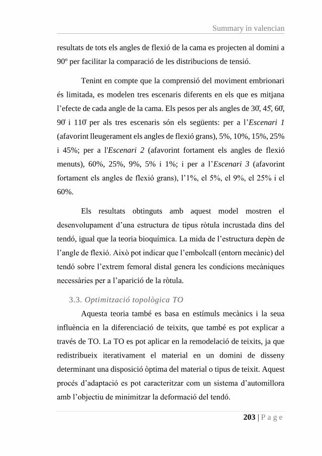
Summary in valencian
203 | P a g e
resultats de tots els angles de flexió de la cama es projecten al domini a
90º per facilitar la comparació de les distribucions de tensió.
Tenint en compte que la comprensió del moviment embrionari
és limitada, es modelen tres escenaris diferents en els que es mitjana
l’efecte de cada angle de la cama. Els pesos per als angles de 30̊, 45̊, 60̊,
90̊ i 110 ̊ per als tres escenaris són els següents: per a l’Escenari 1
(afavorint lleugerament els angles de flexió grans), 5%, 10%, 15%, 25%
i 45%; per a l'Escenari 2 (afavorint fortament els angles de flexió
menuts), 60%, 25%, 9%, 5% i 1%; i per a l’Escenari 3 (afavorint
fortament els angles de flexió grans), l’1%, el 5%, el 9%, el 25% i el
60%.
Els resultats obtinguts amb aquest model mostren el
desenvolupament d’una estructura de tipus ròtula incrustada dins del
tendó, igual que la teoria bioquímica. La mida de l’estructura depèn de
l’angle de flexió. Això pot indicar que l’embolcall (entorn mecànic) del
tendó sobre l’extrem femoral distal genera les condicions mecàniques
necessàries per a l’aparició de la ròtula.
3.3. Optimització topològica TO
Aquesta teoria també es basa en estímuls mecànics i la seua
influència en la diferenciació de teixits, que també es pot explicar a
través de TO. La TO es pot aplicar en la remodelació de teixits, ja que
redistribueix iterativament el material en un domini de disseny
determinant una disposició òptima del material o tipus de teixit. Aquest
procés d’adaptació es pot caracteritzar com un sistema d’automillora
amb l’objectiu de minimitzar la deformació del tendó.
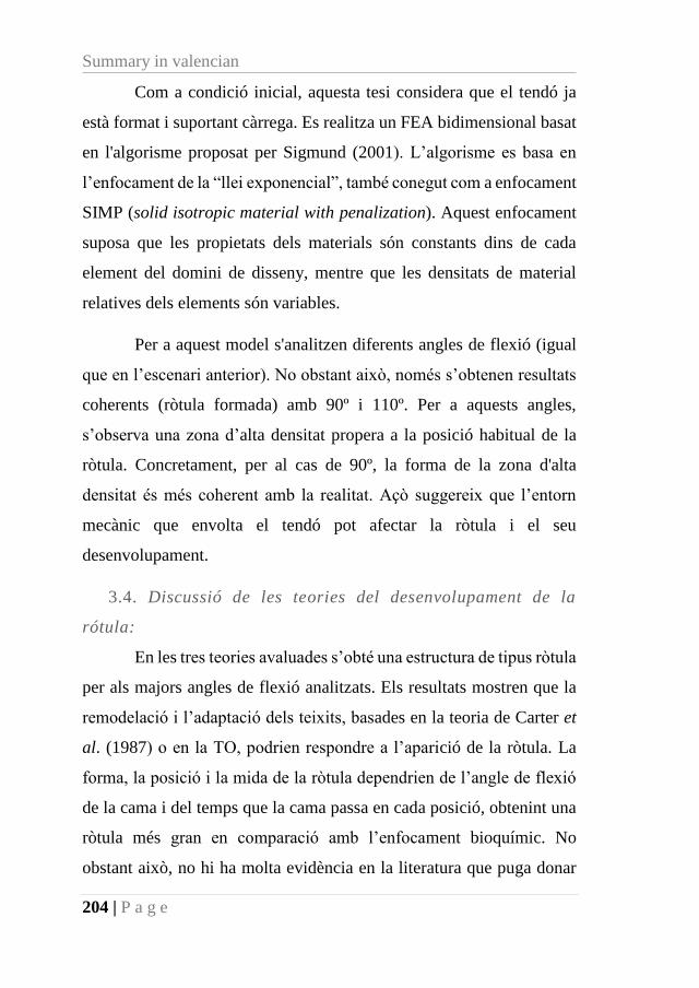
Summary in valencian
204 | P a g e
Com a condició inicial, aquesta tesi considera que el tendó ja
està format i suportant càrrega. Es realitza un FEA bidimensional basat
en l'algorisme proposat per Sigmund (2001). L’algorisme es basa en
l’enfocament de la “llei exponencial”, també conegut com a enfocament
SIMP (solid isotropic material with penalization). Aquest enfocament
suposa que les propietats dels materials són constants dins de cada
element del domini de disseny, mentre que les densitats de material
relatives dels elements són variables.
Per a aquest model s'analitzen diferents angles de flexió (igual
que en l’escenari anterior). No obstant això, només s’obtenen resultats
coherents (ròtula formada) amb 90º i 110º. Per a aquests angles,
s’observa una zona d’alta densitat propera a la posició habitual de la
ròtula. Concretament, per al cas de 90º, la forma de la zona d'alta
densitat és més coherent amb la realitat. Açò suggereix que l’entorn
mecànic que envolta el tendó pot afectar la ròtula i el seu
desenvolupament.
3.4. Discussió de les teories del desenvolupament de la
rótula:
En les tres teories avaluades s’obté una estructura de tipus ròtula
per als majors angles de flexió analitzats. Els resultats mostren que la
remodelació i l’adaptació dels teixits, basades en la teoria de Carter et
al. (1987) o en la TO, podrien respondre a l’aparició de la ròtula. La
forma, la posició i la mida de la ròtula dependrien de l’angle de flexió
de la cama i del temps que la cama passa en cada posició, obtenint una
ròtula més gran en comparació amb l’enfocament bioquímic. No
obstant això, no hi ha molta evidència en la literatura que puga donar
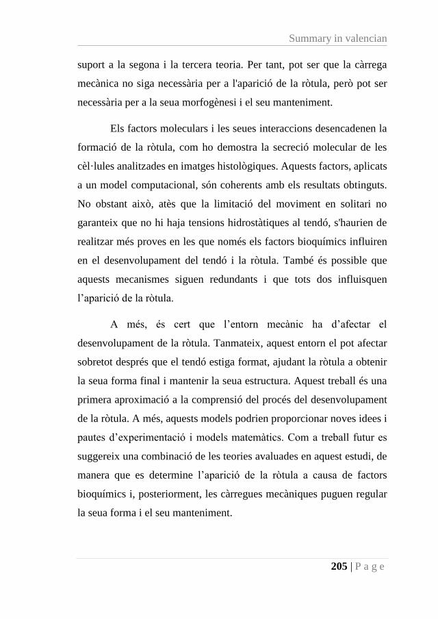
Summary in valencian
205 | P a g e
suport a la segona i la tercera teoria. Per tant, pot ser que la càrrega
mecànica no siga necessària per a l'aparició de la ròtula, però pot ser
necessària per a la seua morfogènesi i el seu manteniment.
Els factors moleculars i les seues interaccions desencadenen la
formació de la ròtula, com ho demostra la secreció molecular de les
cèl·lules analitzades en imatges histològiques. Aquests factors, aplicats
a un model computacional, són coherents amb els resultats obtinguts.
No obstant això, atès que la limitació del moviment en solitari no
garanteix que no hi haja tensions hidrostàtiques al tendó, s'haurien de
realitzar més proves en les que només els factors bioquímics influiren
en el desenvolupament del tendó i la ròtula. També és possible que
aquests mecanismes siguen redundants i que tots dos influisquen
l’aparició de la ròtula.
A més, és cert que l’entorn mecànic ha d’afectar el
desenvolupament de la ròtula. Tanmateix, aquest entorn el pot afectar
sobretot després que el tendó estiga format, ajudant la ròtula a obtenir
la seua forma final i mantenir la seua estructura. Aquest treball és una
primera aproximació a la comprensió del procés del desenvolupament
de la ròtula. A més, aquests models podrien proporcionar noves idees i
pautes d’experimentació i models matemàtics. Com a treball futur es
suggereix una combinació de les teories avaluades en aquest estudi, de
manera que es determine l’aparició de la ròtula a causa de factors
bioquímics i, posteriorment, les càrregues mecàniques puguen regular
la seua forma i el seu manteniment.
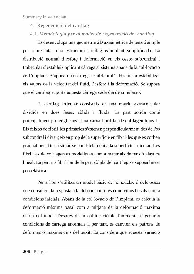
Summary in valencian
206 | P a g e
4. Regeneració del cartílag
4.1. Metodologia per al model de regeneració del cartílag
Es desenvolupa una geometria 2D axisimètrica de tensió simple
per representar una estructura cartílag-os-implant simplificada. La
distribució normal d’esforç i deformació en els ossos subcondral i
trabecular s’estableix aplicant càrrega al sistema abans de la col·locació
de l’implant. S’aplica una càrrega oscil·lant d’1 Hz fins a estabilitzar
els valors de la velocitat del fluid, l’esforç i la deformació. Se suposa
que el cartílag suporta aquesta càrrega cada dia de simulació.
El cartílag articular consisteix en una matriu extracel·lular
dividida en dues fases: sòlida i fluida. La part sòlida conté
principalment proteoglicans i una xarxa fibril·lar de col·lagen tipus II.
Els feixos de fibril·les primàries s'estenen perpendicularment des de l'os
subcondral i divergeixen prop de la superfície en fibril·les que es corben
gradualment fins a situar-se paral·lelament a la superfície articular. Les
fibril·les de col·lagen es modelitzen com a materials de tensió elàstica
lineal. La part no fibril·lar de la part sòlida del cartílag se suposa lineal
poroelàstica.
Per a l'os s’utilitza un model bàsic de remodelació dels ossos
que considera la resposta a la deformació i les condicions basals com a
condicions inicials. Abans de la col·locació de l’implant, es calcula la
deformació màxima basal com a mitjana de la deformació màxima
diària del teixit. Després de la col·locació de l’implant, es generen
condicions de càrrega anormals i, per tant, es canvien els patrons de
deformació màxims dins del teixit. Es considera que aquesta variació
Summary in valencian
207 | P a g e
en les condicions de la deformació afecta la distribució de la densitat
òssia i, per tant, el mòdul de Young dels ossos subcondral i trabecular.
S’estableix que el teixit ossi sota l’implant falla si el mòdul de
Young mitjà de la línia d'elements sota l’implant és menor que un
llindar. Si l'os falla, l’implant es pot desplaçar descendentment dins de
l’os.
També es considera un factor de potencial vascular (potencial
vascularity factor, PVF). Se suposa que aquest factor es difon des del
fons del domini fins a la part superior del domini. Es fixa una taxa de
difusió baixa per a aquesta molècula de manera que determine si un
teixit mesenquimàtic pot ser vascularitzat o no.
El model desenvolupat s'ocupa de la regeneració de dos tipus de
teixits: cartílag i os. El procés d'osteogènesi es regula mitjnaçant
l'entorn mecànic. Per a la regeneració òssia s'utilitza un model mecànic
de diferenciació de teixits que acobla els mecanismes cel·lulars als
estímuls mecànics durant la curació òssia.
Durant la realització d’aquesta tesi no s’han trobat a la literatura
models computacionals capaços d’explicar com es regenera aquest
teixit. Per tant, es considera una relació positiva entre la tensió
hidrostàtica cíclica i el creixement del cartílag. A més, el cartílag només
és capaç de regenerar-se en elements amb teixit mesenquimàtic i baixa
concentració de PVF.
Si l’os sota l’implant falla i es produeix un desplaçament de
l’implant, el buit que queda a la part superior de l’implant s’ompli amb
Summary in valencian
208 | P a g e
teixit mesenquimàtic que, posteriorment, es diferencia en altres teixits
(os, cartílag o teixit fibrós). Per a que un element mesenquimàtic es
diferencie en cartílag, l'element ha d'haver tingut una baixa
concentració de PVF i tindre un element veí cartilaginós amb alta tensió
hidrostàtica. Si no es compleixen les condicions anteriors, s'activa el
model d’osteogènesi. En aquest cas, el teixit mesenquimàtic pot
diferenciar-se en teixits fibrosos, cartílags o ossis en funció dels
estímuls mecànics (efecte combinat de la deformació deviatòrica i la
velocitat del fluid).
4.2. Resultats i discussió del model de regeneració del
cartílag:
Els processos de resorció i aposició òssies es modelitzen com a
canvis en el mòdul de Young de l’os. Segons els resultats, l’os
trabecular s’ha de remodelitzar per suportar la càrrega anormal causada
per l’implant. A més, el mòdul de Young de l’os trabecular augmenta a
la zona sota l’implant un cop s’ha col·locat; però disminueix, a causa
de la sobrecàrrega, a la línia elemental situada just sota l’implant.
D'altra banda, el cartílag es forma a la part superior de l’implant fins al
quart i el sisè mes, quan la concentració del PVF és suficientment alta
per evitar la formació del cartílag.
Quan s'activa el procés d'osteogènesi, l'estímul mecànic calculat
pel model és ideal per estimular el teixit ossi, de manera que només es
diferencia en l'os.
Un any després de la col·locació de l’implant, el model mostra
el cartílag completament recuperat i l’implant desplaçat cap a l’interior
de l'os. Aquests resultats concorden amb els obtinguts per Sancho-Tello
Summary in valencian
209 | P a g e
et al. (2015), qui van col·locar un implant porós de copolímer en
l'articulació del genoll d'un conill per a reparar un defecte condral de
profunditat.
El model computacional desenvolupat en aquesta tesi es pot
utilitzar per a comparar l’efecte d’utilitzar implants de diferents
materials, diferents condicions de càrrega o degeneració (patologia) de
teixits respecte a condicions de tractament ideals. També pot ser útil en
la planificació de tractaments per a la regeneració del cartílag articular.
5. General Conclusions
En aquesta tesi s’exploren diferents aspectes de les articulacions
sinovials des de la seua aparició fins la seua maduresa. Concretament,
es proposen quatre models computacionals basats en factors mecànics i
bioquímics per a reproduir el desenvolupament de les articulacions
sinovials i la regeneració del cartílag articular. En general, els resultats
obtinguts de les simulacions mostren una gran concordança amb els
estudis histològics trobats a la literatura. Les conclusions específiques
extretes de cada model s’exposen a continuació.
El model per a l’aparició d’articulacions es capaç d’explicar el
desenvolupament de l’articulació interfalàngica a través de la interacció
de només sis factors moleculars genèrics. Per tant, es pot concloure que
la concentració de sis molècules relacionades amb GDF-5, Noggin, Ihh,
PTHrP, gens How i Wnt regula la formació de la interzona i el procés
de cavitació.
El model de morfogènesi d’articulacions proposat en aquesta
tesi, a diferència d’altres models computacionals anteriors, inclou
Summary in valencian
210 | P a g e
factors bioquímics a més de factors mecànics. Açò resulta en un grau
d’acord entre la forma final de l’articulació sinovial interfalàngica
simulada i les formes mostrades en estudis histològics notablement
major. Per tant, es demostra que tant els estímuls mecànics com els
bioquímics són necessaris per a que les articulacions sinovials
assolisquen la seua forma final.
Pel que fa a l’aparició de la ròtula, s’avaluen tres teories,
cadascuna implementada mitjançant un model computacional diferent.
Els tres models són capaços de predir l’aparició d’aquest os sesamoide
i, comparant amb els estudis histològics més recents trobats a la
literatura, els millors resultats s’obtenen amb la teoria bioquímica. En
aquesta tesi es proposa que la interacció molecular desencadena
l’aparició de la ròtula, però les càrregues mecàniques són necessàries
per al seu creixement i el seu manteniment.
Segons els resultats del model de regeneració del cartílag, no
només el cartílag s’ha d’adaptar durant el procés de regeneració, sinó
també el teixit que l’envolta. El model computacional desenvolupat pot
resultar útil per a comparar l’efecte d’implants de diferents materials i
de diferents condicions de càrrega i així avaluar quina alternativa és la
més convenient en cada cas.
Els models computacionals desenvolupats en aquesta tesis
permeten avaluar moltes condicions mecàniques i bioquímiques
diferents en diversos fenòmens biològics sense la necessitat de cap
muntatge experimental (amb les dificultats tècniques, costos materials
i econòmics i temps que implicarien). A més, tenen el potencial de
convertir-se en ferramentes útils per a la recerca mèdica i biològica,
Summary in valencian
211 | P a g e
ajudant en el disseny d’estratègies terapèutiques per a les patologies
relacionades amb les articulacions.

213 | P a g e
REFERENCES
[1] D. Correa, S.A. Lietman, Articular cartilage repair: Current needs, methods
and research directions, Semin. Cell Dev. Biol. 62 (2017) 67–77.
doi:10.1016/j.semcdb.2016.07.013.
[2] E. Hohmann, K. Tetsworth, Large osteochondral lesions of the femoral
condyles: Treatment with fresh frozen and irradiated allograft using the Mega
OATS technique, Knee. 23 (2016) 436–441. doi:10.1016/j.knee.2016.01.020.
[3] K.L. Caldwell, J. Wang, Cell-based articular cartilage repair: The link
between development and regeneration, Osteoarthr. Cartil. 23 (2015) 351–
362. doi:10.1016/j.joca.2014.11.004.
[4] M. Sancho-Tello, F. Forriol, P. Gastaldi, A. Ruiz-Saurí, J.J. Martín de Llano,
E. Novella-Maestre, C.M. Antolinos-Turpín, J.A. Gómez-Tejedor, J.L.
Gómez Ribelles, C. Carda, Time evolution of in vivo articular cartilage repair
induced by bone marrow stimulation and scaffold implantation in rabbits, Int.
J. Artif. Organs. 38 (2015) 210–223. doi:10.5301/ijao.5000404.
[5] H. Guo, S.A. Maher, P.A. Torzilli, A biphasic multiscale study of the
mechanical microenvironment of chondrocytes within articular cartilage
under unconfined compression, J. Biomech. 47 (2014) 2721–2729.
doi:10.1016/j.jbiomech.2014.05.001.
[6] S.R. Moore, G.M. Saidel, U. Knothe, M.L. Knothe Tate, Mechanistic,
Mathematical Model to Predict the Dynamics of Tissue Genesis in Bone
Defects via Mechanical Feedback and Mediation of Biochemical Factors,
PLoS Comput. Biol. 10 (2014). doi:10.1371/journal.pcbi.1003604.
[7] D.R. Carter, G.S. Beaupré, N.J. Giori, J.A. Helms, Mechanobiology of
skeletal regeneration, Clin. Orthop. Relat. Res. (1998) S41–S55.
http://eutils.ncbi.nlm.nih.gov/entrez/eutils/elink.fcgi?dbfrom=pubmed&id=9
917625&retmode=ref&cmd=prlinks%5Cnpapers3://publication/uuid/A49B3
192-CFAA-4EE2-86BA-95563B2811A4.
[8] J.M. Guevara, M.A. Moncayo, J.J. Vaca-González, M.L. Gutirrez, L.A.
Barrera, D.A. Garzón-Alvarado, Growth plate stress distribution implications
during bone development: A simple framework computational approach,
Comput. Methods Programs Biomed. 118 (2015) 59–68.
doi:10.1016/j.cmpb.2014.10.007.
[9] D.A. Garzón-Alvarado, J.M. García-Aznar, M. Doblaré, A reaction-diffusion
model for long bones growth, Biomech. Model. Mechanobiol. 8 (2009) 381–
95. doi:10.1007/s10237-008-0144-z.
References
214 | P a g e
[10] T. Miura, P.K. Maini, Periodic pattern formation in reaction–diffusion
systems: An introduction for numerical simulation Introduction: Periodic
pattern formation in biological systems and the Turing reaction–diffusion
model, Anat. Sci. Int. 79 (2004) 112–123. doi:10.1111/j.1447-
073x.2004.00079.x.
[11] A. Madzvamuse, Time-stepping schemes for moving grid finite elements
applied to reaction-diffusion systems on fixed and growing domains, J.
Comput. Phys. 214 (2006) 239–263. doi:10.1016/j.jcp.2005.09.012.
[12] A. Madzvamuse, P.K. Maini, Velocity-induced numerical solutions of
reaction-diffusion systems on continuously growing domains, J. Comput.
Phys. 225 (2007) 100–119. doi:10.1016/j.jcp.2006.11.022.
[13] D.A. Garzón-Alvarado, J.M. García-Aznar, M. Doblaré, Appearance and
location of secondary ossification centres may be explained by a reaction-
diffusion mechanism, Comput. Biol. Med. 39 (2009) 554–561.
doi:10.1016/j.compbiomed.2009.03.012.
[14] D.A. Garzón-Alvarado, A.M.R. Martinez, D.L.L. Segrera, A model of
cerebral cortex formation during fetal development using reaction-diffusion-
convection equations with Turing space parameters, Comput. Methods
Programs Biomed. 104 (2011) 489–497. doi:10.1016/j.cmpb.2011.07.001.
[15] K. Kristiansen, Reaction-Diffusion Models in Mathematical Biology,
Technical University of Denmark, 2008.
[16] S.A. Newman, S. Christley, T. Glimm, H.G.E. Hentschel, B. Kazmierczak,
Y.-T. Zhang, J. Zhu, M.S. Alber, Multiscale Models for Vertebrate Limb
Development, Curr. Top. Dev. Biol. 90 (2008) 979–990. doi:10.1016/S0070-
2153(07)81011-8.
[17] L.P. Räsänen, M.E. Mononen, M.T. Nieminen, E. Lammentausta, J.S.
Jurvelin, R.K. Korhonen, Implementation of subject-specific collagen
architecture of cartilage into a 2D computational model of a knee joint-data
from the osteoarthritis initiative (OAI), J. Orthop. Res. 31 (2013) 10–22.
doi:10.1002/jor.22175.
[18] T.A.M. Heck, W. Wilson, J. Foolen, A.C. Cilingir, K. Ito, C.C. van
Donkelaar, A tissue adaptation model based on strain-dependent collagen
degradation and contact-guided cell traction, J. Biomech. 48 (2015) 823–831.
doi:10.1016/j.jbiomech.2014.12.023.
[19] J.M.P. Quiroga, K. Ito, C.C. van Donkelaar, Meniscus replacement: Influence
of geometrical mismatches on chondroprotective capabilities, J. Biomech. 48
(2015) 1371–1376. doi:10.1016/j.jbiomech.2015.02.063.
[20] J.H. Heegaard, G.S. Beaupre, D.R. Carter, G.S. Beaupré, D.R. Carter,
Mechanically modulated cartilage growth may regulate joint surface
morphogenesis, J. Orthop. Res. 17 (1999) 509–517.
doi:10.1002/jor.1100170408.
References
215 | P a g e
[21] M. Giorgi, A. Carriero, S.J. Shefelbine, N.C. Nowlan, Mechanobiological
simulations of prenatal joint morphogenesis., J. Biomech. 47 (2014) 989–95.
doi:10.1016/j.jbiomech.2014.01.002.
[22] L.R. Cochard, Netter’s Atlas Embryology of Human, Updated Ed, Elsevier
Health Sciences, Chicago, Illinois, 2012.
[23] Th.W. Sadler, Langman’s Medical Embryology, 12th ed., Lippincott
Williams & Wilkins, Cambridge, 2012.
[24] OpenStax, Anatomy and Physiology, OpenStax CNX, 2016.
http://cnx.org/contents/[email protected].
[25] F. Geneser, Atlas de Histología, 8th ed., Editorial Medical Panamericana S.A.,
Madrid, 1998.
[26] P. Pustejovsk, Biochemical and mechanical processes in synovial fluid –
modeling, analysis and computational simulations Mathematical, Charles
University in Prague; Heidelberg University, 2012.
[27] L.R. Gale, Biotribological Assessment for Artificial Synovial Joints : The
Role of Boundary Lubrication, Queensland University of Technology, 2007.
[28] D.E. Marcinko, M.D. Dollard, Physical and mechanical properties of joints
(the pathomechanics of articular cartilage degeneration)., J. Foot Surg. 25
(1986) 3–13. http://www.ncbi.nlm.nih.gov/pubmed/3512683.
[29] H.L. Stewart, C.E. Kawcak, The Importance of Subchondral Bone in the
Pathophysiology of Osteoarthritis, Front. Vet. Sci. 5 (2018) 1–9.
doi:10.3389/fvets.2018.00178.
[30] A.M. Säämänen, J.P.A. Arokoski, J.S. Jurvelin, I. Kiviranta, The structure and
regenerative capacity of synovial joint tissues, Regen. Med. Biomater. Repair
Connect. Tissues. (2010) 1–38. doi:10.1533/9781845697792.1.
[31] J.G. Skedros, S.L. Baucom, Mathematical analysis of trabecular “trajectories”
in apparent trajectorial structures: the unfortunate historical emphasis on the
human proximal femur, J. Theor. Biol. 244 (2007) 15–45.
doi:10.1016/j.jtbi.2006.06.029.
[32] T. Aigner, N. Schmitz, S. Söder, Understanding osteoarthritis and other
cartilage diseases, Regen. Med. Biomater. Repair Connect. Tissues. (2010)
155–177. doi:10.1533/9781845697792.1.155.
[33] J. Fish, T. Belytschko, A First Course in Finite Elements, John Wiley & Sons,
Ltd, Chichester, UK, 2007. doi:10.1002/9780470510858.
[34] M. Pacifici, E. Koyama, M. Iwamoto, Mechanisms of synovial joint and
articular cartilage formation: Recent advances, but many lingering mysteries,
Birth Defects Res. Part C - Embryo Today Rev. 75 (2005) 237–248.
doi:10.1002/bdrc.20050.
References
216 | P a g e
[35] H. Yasuda, B. de Crombrugghe, Joint Formation Requires Muscle Formation
and Contraction, Dev. Cell. 16 (2009) 625–626.
doi:10.1016/j.devcel.2009.05.003.
[36] A.M. Nalin, T.K. Greenlee, L.J. Sandell, Collagen gene expression during
development of avian synovial joints: transient expression of types II and XI
collagen genes in the joint capsule., Dev. Dyn. 203 (1995) 352–362.
doi:10.1002/aja.1002030307.
[37] S. Kimura, K. Shiota, Sequential changes of programmed cell death in
developing fetal mouse limbs and its possible roles in limb morphogenesis, J.
Morphol. 229 (1996) 337–346. doi:10.1002/(SICI)1097-
4687(199609)229:3<337::AID-JMOR8>3.0.CO;2-V.
[38] G. Abu-Hijleh, O. Reid, R.J. Scothorne, Cell death in the developing chick
knee joint: I. Spatial and temporal patterns, Clin. Anat. 10 (1997) 183–200.
doi:10.1002/(SICI)1098-2353(1997)10:3<183::AID-CA4>3.0.CO;2-V.
[39] R. Bellairs, M. Osmond, Atlas of Chick Development, 2nd ed., Elsevier
Science, 2005.
[40] N.C. Nowlan, C. Bourdon, G. Dumas, S. Tajbakhsh, P.J. Prendergast, P.
Murphy, Developing bones are differentially affected by compromised
skeletal muscle formation., Bone. 46 (2010) 1275–85.
doi:10.1016/j.bone.2009.11.026.
[41] F. Accio, C. Bari, F.P. Luyten, Molecular basis of joint development,
Japanese J. Rheumatol. 9 (1999) 17–29. doi:10.1007/BF03041256.
[42] S.E. Stasko, G.F. Wagner, Possible roles for stanniocalcin during early
patterning and joint formation in the mouse, J. Endocrinol. 171 (2001) 237–
248. doi:10.1677/joe.0.1710237.
[43] G. Lizarraga, A. Lichtler, W.B. Upholt, R.A. Kosher, Studies on the role of
Cux1 in regulation of the onset of joint formation in the developing limb, Dev.
Biol. 243 (2002) 44–54. doi:10.1006/dbio.2001.0559.
[44] M. Pacifici, M. Liu, E. Koyama, Joint formation: new findings shed more light
on this critical process in skeletogenesis, Curr. Opin. Orthop. 13 (2002) 339–
344. doi:10.1097/00001433-200210000-00003.
[45] C.W. Archer, G.P. Dowthwaite, P. Francis-West, Development of synovial
joints, Birth Defects Res. Part C - Embryo Today Rev. 69 (2003) 144–155.
doi:10.1002/bdrc.10015.
[46] I.M. Khan, S.N. Redman, R. Williams, G.P. Dowthwaite, S.F. Oldfield, C.W.
Archer, The Development of Synovial Joints, Curr. Top. Dev. Biol. 79 (2007)
1–36. doi:10.1016/S0070-2153(06)79001-9.
[47] N.C. Nowlan, J. Sharpe, K.A. Roddy, P.J. Prendergast, P. Murphy,
Mechanobiology of embryonic skeletal development: Insights from animal
models, Birth Defects Res. Part C Embryo Today Rev. 90 (2010) 203–213.
References
217 | P a g e
doi:10.1002/bdrc.20184.
[48] F. Witte, J. Dokas, F. Neuendorf, S. Mundlos, S. Stricker, Comprehensive
expression analysis of all Wnt genes and their major secreted antagonists
during mouse limb development and cartilage differentiation, Gene Expr.
Patterns. 9 (2009) 215–223. doi:10.1016/j.gep.2008.12.009.
[49] K.L. Cooper, Self-organization in the limb: a Turing mechanism for digit
development, Curr. Opin. Genet. Dev. 32 (2015) 92–97.
doi:10.1016/j.gde.2015.02.001.
[50] W. Schlegel, C. Albrecht, P. Eckl, H. Freudenthaler, A. Berger, V. Vécsei, S.
Marlovits, Dedifferentiation of human articular chondrocytes is associated
with alterations in expression patterns of GDF-5 and its receptors, J. Cell.
Mol. Med. 13 (2009) 3398–3404. doi:10.1111/j.1582-4934.2009.00953.x.
[51] E.E. Storm, D.M. Kingsley, GDF5 coordinates bone and joint formation
during digit development, Dev. Biol. 209 (1999) 11–27.
doi:10.1006/dbio.1999.9241.
[52] E. Kavanagh, V.L. Church, A.C. Osborne, K.J. Lamb, C.W. Archer, P.H.
Francis-West, A.A. Pitsillides, Differential regulation of GDF-5 and FGF-2/4
by immobilisation in ovo exposes distinct roles in joint formation, Dev. Dyn.
235 (2006) 826–834. doi:10.1002/dvdy.20679.
[53] S. Provot, E. Schipani, Molecular mechanisms of endochondral bone
development, Biochem. Biophys. Res. Commun. 328 (2005) 658–665.
doi:10.1016/j.bbrc.2004.11.068.
[54] J.E.M. Brouwers, C.C. van Donkelaar, B.G. Sengers, R. Huiskes, Can the
growth factors PTHrP, Ihh and VEGF, together regulate the development of
a long bone?, J. Biomech. 39 (2006) 2774–2782.
doi:10.1016/j.jbiomech.2005.10.004.
[55] D.A. Garzón-Alvarado, L.M. Peinado Cortés, R.P. Cárdenas Sandoval, A
mathematical model of epiphyseal development: hypothesis of growth pattern
of the secondary ossification centre., Comput. Methods Biomech. Biomed.
Engin. 14 (2011) 23–32. doi:10.1080/10255842.2010.484810.
[56] L.M. Peinado Cortés, J.C. Vanegas Acosta, D.A. Garzón Alvarado, A
mechanobiological model of epiphysis structures formation., J. Theor. Biol.
287 (2011) 13–25. doi:10.1016/j.jtbi.2011.07.011.
[57] F.P. Luyten, P. Tylzanowski, R.J. Lories, Wnt signaling and osteoarthritis,
Bone. 44 (2009) 522–527. doi:10.1016/j.bone.2008.12.006.
[58] A.M. Turing, The Chemical Basis of Morphogenesis, Philos. Trans. R. Soc.
Lond. B. Biol. Sci. 237 (1952) 37–72. doi:10.1098/rstb.1952.0012.
[59] J.D. Murray, A Pre-pattern formation mechanism for animal coat markings,
J. Theor. Biol. 88 (1981) 161–199. doi:10.1016/0022-5193(81)90334-9.
References
218 | P a g e
[60] A. Madzvamuse, A Numerical Approach to the Study of Spatial Pattern
Formation, Oxford University, 2000.
[61] D.M. Wellik, M.R. Capecchi, Hox10 and Hox11 genes are required to
globally pattern the mammalian skeleton., Science. 301 (2003) 363–367.
doi:10.1126/science.1085672.
[62] P. Dollé, E. Ruberte, P. Kastner, M. Petkovich, C.M. Stoner, L.J. Gudas, P.
Chambon, Differential expression of genes encoding α, β and γ retinoic acid
receptors and CRABP in the developing limbs of the mouse, Nature. 342
(1989) 702–705. doi:10.1038/342702a0.
[63] Y. Yokouchi, H. Sasaki, A. Kuroiwa, Homeobox gene expression correlated
with the bifurcation process of limb cartilage development, Nature. 353
(1991) 443–445. doi:10.1038/353443a0.
[64] C.E. Nelson, B.A. Morgan, A.C. Burke, E. Laufer, E. DiMambro, L.C.
Murtaugh, E. Gonzales, L. Tessarollo, L.F. Parada, C. Tabin, Analysis of Hox
gene expression in the chick limb bud., Development. 122 (1996) 1449–1466.
[65] A. Badugu, C. Kraemer, P. Germann, D. Menshykau, D. Iber, Digit patterning
during limb development as a result of the BMP-receptor interaction, Sci.
Rep. 2 (2012) 991. doi:10.1038/srep00991.
[66] J.M. Kindblom, O. Nilsson, T. Hurme, C. Ohlsson, L. Savendahl, Expression
and localization of Indian hedgehog (Ihh) and parathyroid hormone-related
protein (PTHrP) in the human growth plate during pubertal development, J.
Endocrinol. 174 (2002) 1–6. doi:10.1677/joe.0.174R001.
[67] B. St-Jacques, M. Hammerschmidt, A.P. McMahon, Indian hedgehog
signaling regulates proliferation and differentiation of chondrocytes and is
essential for bone formation., Genes Dev. 13 (1999) 2072–2086.
doi:10.1101/gad.13.16.2072.
[68] E. Zelzer, B.R. Olsen, The genetic basis for skeletal diseases., Nature. 423
(2003) 343–348. doi:10.1038/nature01659.
[69] E. KOYAMA, T. OCHIAI, R.B. ROUNTREE, D.M. KINGSLEY, M.
ENOMOTO-IWAMOTO, M. IWAMOTO, M. PACIFICI, Synovial Joint
Formation during Mouse Limb Skeletogenesis: Roles of Indian Hedgehog
Signaling, Ann. N. Y. Acad. Sci. 1116 (2007) 100–112.
doi:10.1196/annals.1402.063.
[70] D. Mitrovic, Development of the diarthrodial joints in the rat embryo, Am. J.
Anat. 151 (1978) 475–485. doi:10.1002/aja.1001510403.
[71] Y.-T. Zhang, M.S. Alber, S.A. Newman, R.H. Dillon, Mathematical modeling
of vertebrate limb development., Math. Biosci. 243 (2013) 1–17.
doi:10.1016/j.mbs.2012.11.003.
[72] S.A. Newman, R. Bhat, Activator-inhibitor dynamics of vertebrate limb
pattern formation, Birth Defects Res. Part C - Embryo Today Rev. 81 (2007)
References
219 | P a g e
305–319. doi:10.1002/bdrc.20112.
[73] R. Chaturvedi, C. Huang, B. Kazmierczak, T. Schneider, J.A. Izaguirre, T.
Glimm, H.G.E. Hentschel, J.A. Glazier, S.A. Newman, M.S. Alber, On
multiscale approaches to three-dimensional modelling of morphogenesis, J.
R. Soc. Interface. 2 (2005) 237–253. doi:10.1098/rsif.2005.0033.
[74] J.D. Murray, Mathematical Biology II: Spatial Models and Biomedical
Applications, Springer-Verlag, New York, 1993. doi:10.1007/b98869.
[75] B. Boehm, H. Westerberg, G. Lesnicar-Pucko, S. Raja, M. Rautschka, J.
Cotterell, J. Swoger, J. Sharpe, The Role of Spatially Controlled Cell
Proliferation in Limb Bud Morphogenesis, PLoS Biol. 8 (2010) e1000420.
doi:10.1371/journal.pbio.1000420.
[76] A. Goriely, The Mathematics and Mechanics of Biological Growth, Springer
New York, New York, NY, 2017. doi:10.1007/978-0-387-87710-5.
[77] R. Merino, D. Macias, Y. Gañan, A.N. Economides, X. Wang, Q. Wu, N.
Stahl, K.T. Sampath, P. Varona, J.M. Hurle, Expression and function of Gdf-
5 during digit skeletogenesis in the embryonic chick leg bud, Dev. Biol. 206
(1999) 33–45. doi:10.1006/dbio.1998.9129.
[78] E. Koyama, Y. Shibukawa, M. Nagayama, H. Sugito, B. Young, T. Yuasa, T.
Okabe, T. Ochiai, N. Kamiya, R.B. Rountree, D.M. Kingsley, M. Iwamoto,
M. Enomoto-Iwamoto, M. Pacifici, A distinct cohort of progenitor cells
participates in synovial joint and articular cartilage formation during mouse
limb skeletogenesis, Dev. Biol. 316 (2008) 62–73.
doi:10.1016/j.ydbio.2008.01.012.
[79] F.R. Bailey, A.M. Miller, Embryology, William Wood and Co., New York,
1921.
[80] J. Raspopovic, L. Marcon, L. Russo, J. Sharpe, Digit patterning is controlled
by a Bmp-Sox9-Wnt Turing network modulated by morphogen gradients,
Science (80-. ). 345 (2014) 566–570. doi:10.1126/science.1252960.
[81] B. Gao, J. Hu, S. Stricker, M. Cheung, G. Ma, K.F. Law, F. Witte, J. Briscoe,
S. Mundlos, L. He, K.S.E. Cheah, D. Chan, A mutation in Ihh that causes digit
abnormalities alters its signalling capacity and range., Nature. 458 (2009)
1196–1200. doi:10.1038/nature07862.
[82] C. Hartmann, C.J. Tabin, Wnt-14 plays a pivotal role in inducing synovial
joint formation in the developing appendicular skeleton, Cell. 104 (2001)
341–351. doi:10.1016/S0092-8674(01)00222-7.
[83] R.S. Decker, E. Koyama, M. Enomoto-Iwamoto, P. Maye, D. Rowe, S. Zhu,
P.G. Schultz, M. Pacifici, Mouse limb skeletal growth and synovial joint
development are coordinately enhanced by Kartogenin, Dev. Biol. 395 (2014)
255–267. doi:10.1016/j.ydbio.2014.09.011.
References
220 | P a g e
[84] K.D. Kavanagh, O. Shoval, B.B. Winslow, U. Alon, B.P. Leary, A. Kan, C.J.
Tabin, Developmental bias in the evolution of phalanges, Proc. Natl. Acad.
Sci. 110 (2013) 18190–18195. doi:10.1073/pnas.1315213110.
[85] P.H. Francis-West, J. Parish, K. Lee, C.W. Archer, BMP/GDF-signalling
interactions during synovial joint development, Cell Tissue Res. 296 (1999)
111–119. doi:10.1007/s004410051272.
[86] N.C. Nowlan, J. Sharpe, Joint shape morphogenesis precedes cavitation of the
developing hip joint, J. Anat. 224 (2014) 482–489. doi:10.1111/joa.12143.
[87] V. Bialik, G.M. Bialik, S. Blazer, P. Sujov, F. Wiener, M. Berant,
Developmental Dysplasia of the Hip: A New Approach to Incidence,
Pediatrics. 103 (1999) 93–99. doi:10.1542/peds.103.1.93.
[88] A. Fassier, P. Wicart, J. Dubousset, R. Seringe, Arthrogryposis multiplex
congenita. Long-term follow-up from birth until skeletal maturity, J. Child.
Orthop. 3 (2009) 383–390. doi:10.1007/s11832-009-0187-4.
[89] D.J. Gray, E. Gardner, Prenatal development of the human knee and superior
tibiofibular joints, Am. J. Anat. 86 (1950) 235–287.
doi:10.1002/aja.1000860204.
[90] E. Gardner, R. O’Rahilly, The early development of the knee joint in staged
human embryos, J. Anat. 102 (1968) 289–299.
http://www.ncbi.nlm.nih.gov/pubmed/5643844.
[91] D.R. Carter, Mechanical loading history and skeletal biology, J. Biomech. 20
(1987) 1095–1109. doi:10.1016/0021-9290(87)90027-3.
[92] D.R. Carter, P.R. Blenman, G.S. Beauprk, Correlations between Mechanical
Stress History and Tissue Differentiation in Initial Fracture Healing, J.
Orthop. Res. 6 (1988) 736–748. doi:10.1002/jor.1100060517.
[93] D.R. Carter, M. Wong, The role of mechanical loading histories in the
development of diarthrodial joints, J. Orthop. Res. 6 (1988) 804–816.
doi:10.1002/jor.1100060604.
[94] E.L. Radin, D.B. Burr, B. Caterson, D. Fyhrie, T.D. Brown, R.D. Boyd,
Mechanical Determinants of Osteoarthrosis, Semin. Arthritis Rheum. 21
(1991) 12–21. doi:10.1016/0049-0172(91)90036-Y.
[95] P.N.P. Singh, C.A. Shea, S.K. Sonker, R.A. Rolfe, A. Ray, S. Kumar, P.
Gupta, P. Murphy, A. Bandyopadhyay, Precise spatial restriction of BMP
signaling in developing joints is perturbed upon loss of embryo movement,
Development. 145 (2018) dev153460. doi:10.1242/dev.153460.
[96] K.M. Márquez-Flórez, J.R. Monaghan, S.J. Shefelbine, A. Ramirez-Martínez,
D.A. Garzón-Alvarado, A computational model for the joint onset and
development, J. Theor. Biol. 454 (2018) 345–356.
doi:10.1016/j.jtbi.2018.04.015.

References
221 | P a g e
[97] K.M. Márquez-Flórez, O. Silva, C.A. Narváez-Tovar, D.A. Garzón-alvarado,
A Comparison of the Contact Force Distributions on the Acetabular Surface
Due to Orthopedic Treatments for Developmental Hip Dysplasia, J. Biomech.
Eng. 138 (2016) 074501-1-074501–7. doi:10.1115/1.4033547.
[98] K.A. Roddy, P.J. Prendergast, P. Murphy, Mechanical influences on
morphogenesis of the knee joint revealed through morphological, molecular
and computational analysis of immobilised embryos, PLoS One. 6 (2011).
doi:10.1371/journal.pone.0017526.
[99] A.C. Osborne, K.J. Lamb, J.C. Lewthwaite, G.P. Dowthwaite, A.A.
Pitsillides, Short-term rigid and flaccid paralyses diminish growth of
embryonic chick limbs and abrogate joint cavity formation but differentially
preserve pre-cavitated joints., J. Musculoskelet. Neuronal Interact. 2 (2002)
448–456. http://www.ncbi.nlm.nih.gov/pubmed/15758413.
[100] B. Mikic, T.L. Johnson, A.B. Chhabra, B.J. Schalet, M. Wong, E.B. Hunziker,
Differential effects of embryonic immobilization on the development of
fibrocartilaginous skeletal elements., J. Rehabil. Res. Dev. 37 (2000) 127–33.
http://www.ncbi.nlm.nih.gov/pubmed/10850818.
[101] J. Kahn, Y. Shwartz, E. Blitz, S. Krief, A. Sharir, D.A. Breitel, R. Rattenbach,
F. Relaix, P. Maire, R.B. Rountree, D.M. Kingsley, E. Zelzer, Muscle
Contraction Is Necessary to Maintain Joint Progenitor Cell Fate, Dev. Cell.
16 (2009) 734–743. doi:10.1016/j.devcel.2009.04.013.
[102] N.C. Nowlan, J. Sharpe, K. a. Roddy, P.J. Prendergast, P. Murphy,
Mechanobiology of embryonic skeletal development: Insights from animal
models., Birth Defects Res. C. Embryo Today. 90 (2010) 203–13.
doi:10.1002/bdrc.20184.
[103] D.R. Carter, T.E. Orr, D.P. Fyhrie, D.J. Schurman, Influences of mechanical
stress on prenatal and postnatal skeletal development., Clin. Orthop. Relat.
Res. No. 219 (1987) 237–50. http://www.ncbi.nlm.nih.gov/pubmed/3581576.
[104] N. Burton-Wurster, M. Vernier-Singer, T. Farquhar, G. Lust, Effect of
compressive loading and unloading on the synthesis of total protein,
proteoglycan, and fibronectin by canine cartilage explants, J. Orthop. Res. 11
(1993) 717–729. doi:10.1002/jor.1100110514.
[105] F. Guilak, B. Meyer, A. Ratcliffe, V. Mow, The effects of matrix compression
on proteoglycan metabolism in articular cartilage explants, Osteoarthr. Cartil.
2 (1994) 91–101. doi:10.1016/S1063-4584(05)80059-7.
[106] Y.J. Kim, R.L.Y. Sah, A.J. Grodzinsky, A.H.K. Plaas, J.D. Sandy,
Mechanical Regulation of Cartilage Biosynthetic Behavior: Physical Stimuli,
Arch. Biochem. Biophys. 311 (1994) 1–12. doi:10.1006/abbi.1994.1201.
[107] T.H. Korver, R.J. van de Stadt, E. Kiljan, G.P. van Kampen, J.K. van der
Korst, Effects of loading on the synthesis of proteoglycans in different layers
References
222 | P a g e
of anatomically intact articular cartilage in vitro., J. Rheumatol. 19 (1992)
905–12. http://www.ncbi.nlm.nih.gov/pubmed/1404127.
[108] J.J. Parkkinen, M.J. Lammi, H.J. Helminen, M. Tammi, Local stimulation of
proteoglycan synthesis in articular cartilage explants by dynamic compression
in vitro, J. Orthop. Res. 10 (1992) 610–620. doi:10.1002/jor.1100100503.
[109] P.H. Francis-West, A. Abdelfattah, P. Chen, C. Allen, J. Parish, R. Ladher, S.
Allen, S. MacPherson, F.P. Luyten, C.W. Archer, Mechanisms of GDF-5
action during skeletal development., Development. 126 (1999) 1305–15.
http://www.ncbi.nlm.nih.gov/pubmed/10021348.
[110] Y.Q. Yang, Y.Y. Tan, R. Wong, A. Wenden, L.K. Zhang, A.B.M. Rabie, The
role of vascular endothelial growth factor in ossification, Int. J. Oral Sci. 4
(2012) 64–68. doi:10.1038/ijos.2012.33.
[111] S.E. Usmani, M.A. Pest, G. Kim, S.N. Ohora, L. Qin, F. Beier, Transforming
growth factor alpha controls the transition from hypertrophic cartilage to bone
during endochondral bone growth, Bone. 51 (2012) 131–141.
doi:10.1016/j.bone.2012.04.012.
[112] X. Guo, K.K. Mak, M.M. Taketo, Y. Yang, The Wnt/β-catenin pathway
interacts differentially with PTHrP signaling to control chondrocyte
hypertrophy and final maturation, PLoS One. 4 (2009).
doi:10.1371/journal.pone.0006067.
[113] D.R. Carter, G.S. Beaupré, M. Wong, R.L. Smith, T.P. Andriacchi, D.J.
Schurman, The mechanobiology of articular cartilage development and
degeneration., Clin. Orthop. Relat. Res. 427 (2004) S69-77.
doi:10.1097/01.blo.0000144970.05107.7e.
[114] V. Sarin, D. Carter, Mechanobiology and joint conformity regulate
endochondral ossification of sesamoids., J. Orthop. Res. 18 (2000) 706–712.
doi:10.1002/jor.1100180505.
[115] J.C.V. Acosta, D.A. Garzón-Alvarado, L.M.P. Corte, A mechanobiological
model of epiphysis structures formation, J. Theor. Biol. 287 (2011) 13–25.
doi:10.1016/j.jtbi.2011.07.011.
[116] D.R. Carter, M. Wong, Modelling cartilage mechanobiology, Philos. Trans.
R. Soc. Lond. B. Biol. Sci. 358 (2003) 1461–1471.
doi:10.1098/rstb.2003.1346.
[117] S. Eyal, E. Blitz, Y. Shwartz, H. Akiyama, S. Ronen, E. Zelzer, On the
development of the patella, Development. (2015) 1–9.
doi:10.1242/dev.121970.
[118] F.S. Sutton, C.H. Thompson, J. Lipke, D.B. Kettelkamp, The effect of
patellectomy on knee function., J. Bone Joint Surg. Am. 58 (1976) 537–540.
http://www.ncbi.nlm.nih.gov/pubmed/1270472.
[119] O.S. Schindler, W.N. Scott, Basic kinematics and biomechanics of the patello-
References
223 | P a g e
femoral joint. Part 1: The native patella., Acta Orthop. Belg. 77 (2011) 421–
31. http://www.ncbi.nlm.nih.gov/pubmed/21954748.
[120] S. Mottershead, Sesamoid bones and cartilages: An enquiry into their
function, Clin. Anat. 1 (1988) 59–62. doi:10.1002/ca.980010110.
[121] D.S. Howale, Z.K. Patel, Hypothesis : Morphology & Development of
Patella, Int. J. Sci. Res. Publ. 3 (2013) 1–5.
[122] I.G. Jang, I.Y. Kim, Application of design space optimization to bone
remodeling simulation of trabecular architecture in human proximal femur for
higher computational efficiency, Finite Elem. Anal. Des. 46 (2010) 311–319.
doi:10.1016/j.finel.2009.11.003.
[123] K. Cai, Z. Luo, Y. Wang, Topology optimization for human proximal femur
considering bi-modulus behavior of cortical bones, Springer Proc. Math. Stat.
95 (2015) 263–270. doi:10.1007/978-3-319-08377-3_26.
[124] P.G. Coelho, P.R. Fernandes, H.C. Rodrigues, J.B. Cardoso, J.M. Guedes,
Numerical modeling of bone tissue adaptation-A hierarchical approach for
bone apparent density and trabecular structure, J. Biomech. 42 (2009) 830–
837. doi:10.1016/j.jbiomech.2009.01.020.
[125] I.G. Jang, I.Y. Kim, Computational study of Wolff’s law with trabecular
architecture in the human proximal femur using topology optimization, J.
Biomech. 41 (2008) 2353–2361. doi:10.1016/j.jbiomech.2008.05.037.
[126] C. Boyle, I.Y. Kim, Three-dimensional micro-level computational study of
Wolff’s law via trabecular bone remodeling in the human proximal femur
using design space topology optimization, J. Biomech. 44 (2011) 935–942.
doi:10.1016/j.jbiomech.2010.11.029.
[127] C.L. Chang, C.S. Chen, C.H. Huang, M.L. Hsu, Finite element analysis of the
dental implant using a topology optimization method, Med. Eng. Phys. 34
(2012) 999–1008. doi:10.1016/j.medengphy.2012.06.004.
[128] H. Kang, C.Y. Lin, S.J. Hollister, Topology optimization of three dimensional
tissue engineering scaffold architectures for prescribed bulk modulus and
diffusivity, Struct. Multidiscip. Optim. 42 (2010) 633–644.
doi:10.1007/s00158-010-0508-8.
[129] A. Sutradhar, G.H. Paulino, M.J. Miller, T.H. Nguyen, Topological
optimization for designing patient-specific large craniofacial segmental bone
replacements, Proc. Natl. Acad. Sci. 107 (2010) 13222–13227.
doi:10.1073/pnas.1001208107.
[130] M. Fraldi, L. Esposito, G. Perrella, A. Cutolo, S.C. Cowin, Topological
optimization in hip prosthesis design, Biomech. Model. Mechanobiol. 9
(2010) 389–402. doi:10.1007/s10237-009-0183-0.
[131] R. Schweitzer, E. Zelzer, T. Volk, Connecting muscles to tendons: tendons
References
224 | P a g e
and musculoskeletal development in flies and vertebrates., Development. 137
(2010) 2807–2817. doi:10.1242/dev.047498.
[132] F. Edom-Vovard, B. Schuler, M.-A. Bonnin, M.-A. Teillet, D. Duprez, Fgf4
positively regulates scleraxis and tenascin expression in chick limb tendons.,
Dev. Biol. 247 (2002) 351–366. doi:10.1006/dbio.2002.0707.
[133] S. Eloy-Trinquet, H. Wang, F. Edom-Vovard, D. Duprez, Fgf signaling
components are associated with muscles and tendons during limb
development, Dev. Dyn. 238 (2009) 1195–1206. doi:10.1002/dvdy.21946.
[134] E. Blitz, A. Sharir, H. Akiyama, E. Zelzer, Tendon-bone attachment unit is
formed modularly by a distinct pool of Scx- and Sox9-positive progenitors,
Development. 140 (2013) 2680–2690. doi:10.1242/dev.093906.
[135] N.J. Giori, G.S. Beaupré, D.R. Carter, Cellular shape and pressure may
mediate mechanical control of tissue composition in tendons, J. Orthop. Res.
11 (1993) 581–591. doi:10.1002/jor.1100110413.
[136] J. Wilkinson, Fracture of the patella treated by total excision. A long-term
follow-up, J. Bone Joint Surg. Br. 59 (1977) 352–354.
http://www.ncbi.nlm.nih.gov/pubmed/893514.
[137] D.R. Carter, P.R. Blenman, G.S. Beaupre, G.S. Beaupré, Correlations
between mechanical-stress history and tissue differentiation in initial fracture-
healing, J. Orthop. Res. 6 (1988) 736–748. doi:10.1002/jor.1100060517.
[138] D.B. Drachman, L. Sokoloff, The role of movement in embryonic joint
development, Dev. Biol. 14 (1966) 401–420. doi:10.1016/0012-
1606(66)90022-4.
[139] T.A. Wren, G.S. Beaupré, D.R. Carter, Mechanobiology of tendon adaptation
to compressive loading through fibrocartilaginous metaplasia, J. Rehabil. Res.
Dev. 37 (2000) 135–143.
[140] H. Aslan, N. Kimelman-Bleich, G. Pelled, D. Gazit, Molecular targets for
tendon neoformation, J. Clin. Invest. 118 (2008) 439–444.
doi:10.1172/JCI33944.
[141] L. Geris, J. Vander Sloten, H. Van Oosterwyck, In silico biology of bone
modelling and remodelling: regeneration, Philos. Trans. R. Soc. A Math.
Phys. Eng. Sci. 367 (2009) 2031–2053. doi:10.1098/rsta.2008.0293.
[142] S. Piszczatowski, Material aspects of growth plate modelling using Carter’s
and Stokes’s approaches., Acta Bioeng. Biomech. 13 (2011) 3–14.
http://www.ncbi.nlm.nih.gov/pubmed/22097913.
[143] W.R. MacAusland, Total excision of the patella for fracture, Am. J. Surg. 72
(1946) 510–516. doi:10.1016/0002-9610(46)90385-6.
[144] J. Bruce, R. Walmsley, Exision of the patella: Some Experimental and
Anatomical Observations, JBJS. 24 (1942) 311–325.
References
225 | P a g e
https://journals.lww.com/jbjsjournal/Fulltext/1942/24020/EXCISION_OF_T
HE_PATELLA__Some_Experimental_and.8.aspx.
[145] O. Sigmund, A 99 line topology optimization code written in matlab, Struct.
Multidiscip. Optim. 21 (2001) 120–127. doi:10.1007/s001580050176.
[146] A. Sutradhar, J. Park, D. Carrau, T.H. Nguyen, M.J. Miller, G.H. Paulino,
Designing patient-specific 3D printed craniofacial implants using a novel
topology optimization method, Med. Biol. Eng. Comput. 54 (2016) 1123–
1135. doi:10.1007/s11517-015-1418-0.
[147] T.A.E. Ahmed, M.T. Hincke, Strategies for Articular Cartilage Lesion Repair
and Functional Restoration, Tissue Eng. Part B Rev. 16 (2010) 305–329.
doi:10.1089/ten.teb.2009.0590.
[148] J.E.J. Bekkers, M. Inklaar, D.B.F. Saris, Treatment Selection in Articular
Cartilage Lesions of the Knee, Am. J. Sports Med. 37 (2009) 148–155.
doi:10.1177/0363546509351143.
[149] N.L. Grimm, J.M. Weiss, J.I. Kessler, S.K. Aoki, Osteochondritis dissecans
of the knee: Pathoanatomy, epidemiology, and diagnosis, Clin. Sports Med.
33 (2014) 181–188. doi:10.1016/j.csm.2013.11.006.
[150] T.M. Simon, D.W. Jackson, Articular Cartilage: Injury Pathways and
Treatment Options, Sports Med. Arthrosc. 26 (2018) 31–39.
doi:10.1097/JSA.0000000000000182.
[151] C.M. Agrawal, R.B. Ray, Biodegradable polymeric scaffolds for
musculoskeletal tissue engineering, J. Biomed. Mater. Res. 55 (2001) 141–
150. doi:10.1002/1097-4636(200105)55:2<141::AID-JBM1000>3.0.CO;2-J.
[152] M. Pérez Olmedilla, N. Garcia-Giralt, M.M. Pradas, P.B. Ruiz, J.L. Gómez
Ribelles, E.C. Palou, J.C.M. García, Response of human chondrocytes to a
non-uniform distribution of hydrophilic domains on poly (ethyl acrylate-co-
hydroxyethyl methacrylate) copolymers, Biomaterials. 27 (2006) 1003–1012.
doi:10.1016/j.biomaterials.2005.07.030.
[153] W.-J. Li, K.G. Danielson, P.G. Alexander, R.S. Tuan, Biological response of
chondrocytes cultured in three-dimensional nanofibrous poly(ϵ-caprolactone)
scaffolds, J. Biomed. Mater. Res. 67A (2003) 1105–1114.
doi:10.1002/jbm.a.10101.
[154] G. Luca, M. Calvitti, C. Nastruzzi, L. Bilancetti, E. Becchetti, G. Angeletti,
F. Mancuso, R. Calafiore, Encapsulation, In Vitro Characterization, and In
Vivo Biocompatibility of Sertoli Cells in Alginate-Based Microcapsules,
Tissue Eng. 13 (2007) 641–648. doi:10.1089/ten.2006.0137.
[155] M. Wong, M. Siegrist, X. Wang, E. Hunziker, Development of mechanically
stable alginate/chondrocyte constructs: effects of guluronic acid content and
matrix synthesis, J. Orthop. Res. 19 (2001) 493–499. doi:10.1016/S0736-
0266(00)90023-8.
References
226 | P a g e
[156] S.R. Frenkel, P.E. Dicesare, Scaffolds for articular cartilage repair, J. Long.
Term. Eff. Med. Implants. 22 (2004) 26–34.
doi:10.1023/B:ABME.0000007788.41804.0d.
[157] B.J. Huang, J.C. Hu, K.A. Athanasiou, Cell-based tissue engineering
strategies used in the clinical repair of articular cartilage, Biomaterials. 98
(2016) 1–22. doi:10.1016/j.biomaterials.2016.04.018.
[158] M. Sancho-Tello, F. Forriol, J.J. Martín de Llano, C. Antolinos-Turpin, J.A.
Gómez-Tejedor, J.L. Gómez Ribelles, C. Carda, Biostable scaffolds of
polyacrylate polymers implanted in the articular cartilage induce hyaline-like
cartilage regeneration in rabbits, Int. J. Artif. Organs. 40 (2017) 350–357.
doi:10.5301/ijao.5000598.
[159] L. Vikingsson, M. Sancho-Tello, A. Ruiz-Saurí, S.M. Díaz, J.A. Gómez-
Tejedor, G.G. Ferrer, C. Carda, J.C. Monllau, J.L. Gómez Ribelles,
Implantation of a polycaprolactone scaffold with subchondral bone anchoring
ameliorates nodules formation and other tissue alterations, Int. J. Artif.
Organs. 38 (2015) 659–666. doi:10.5301/ijao.5000457.
[160] E. Kon, A. Roffi, G. Filardo, G. Tesei, M. Marcacci, Scaffold-based cartilage
treatments: with or without cells? A systematic review of preclinical and
clinical evidence, Arthroscopy. 31 (2015) 767–775.
doi:10.1016/j.arthro.2014.11.017.
[161] M. Cucchiarini, H. Madry, F. Guilak, D. Saris, M. Stoddart, M. Koon Wong,
P. Roughley, A vision on the future of articular cartilage repair, Eur. Cells
Mater. 27s (2014) 12–16. doi:10.22203/eCM.v027sa03.
[162] I. Gadjanski, K. Spiller, G. Vunjak-Novakovic, Time-Dependent Processes in
Stem Cell-Based Tissue Engineering of Articular Cartilage, Stem Cell Rev.
Reports. 8 (2012) 863–881. doi:10.1007/s12015-011-9328-5.
[163] C.J. Little, N.K. Bawolin, X. Chen, Mechanical Properties of Natural
Cartilage and Tissue-Engineered Constructs, Tissue Eng. Part B Rev. 17
(2011) 213–227. doi:10.1089/ten.teb.2010.0572.
[164] L. Vikingsson, G. Gallego Ferrer, J.A. Gómez-Tejedor, J.L. Gómez Ribelles,
An “in vitro” experimental model to predict the mechanical behavior of
macroporous scaffolds implanted in articular cartilage, J. Mech. Behav.
Biomed. Mater. 32 (2014) 125–131. doi:10.1016/j.jmbbm.2013.12.024.
[165] G. Filardo, E. Kon, A. Roffi, A. Di Martino, M. Marcacci, Scaffold-based
repair for cartilage healing: A systematic review and technical note, Arthrosc.
J. Arthrosc. Relat. Surg. 29 (2013) 174–186.
doi:10.1016/j.arthro.2012.05.891.
[166] E. Kon, G. Filardo, A. Roffi, L. Andriolo, M. Marcacci, New trends for knee
cartilage regeneration: From cell-free scaffolds to mesenchymal stem cells,
Curr. Rev. Musculoskelet. Med. 5 (2012) 236–243. doi:10.1007/s12178-012-
9135-x.
References
227 | P a g e
[167] S. Martinez-Diaz, N. Garcia-Giralt, M. Lebourg, J.A. Gómez-Tejedor, G.
Vila, E. Caceres, P. Benito, M. Monleón Pradas, X. Nogues, J.L. Gómez
Ribelles, J.C. Monllau, In Vivo Evaluation of 3-Dimensional
Polycaprolactone Scaffolds for Cartilage Repair in Rabbits, Am. J. Sports
Med. 38 (2010) 509–519. doi:10.1177/0363546509352448.
[168] H. Van Oosterwyck, Computational mechanobiology: may the force be with
you, J. Math. Biol. 70 (2015) 1323–1326. doi:10.1007/s00285-014-0795-6.
[169] T.-H. Lin, H.-Y. Jhang, F.-C. Chu, C.A. Chung, Computational modeling of
nutrient utilization in engineered cartilage, Biotechnol. Prog. 29 (2013) 452–
462. doi:10.1002/btpr.1687.
[170] M.S. Hossain, D.J. Bergstrom, X.B. Chen, Modelling and simulation of the
chondrocyte cell growth, glucose consumption and lactate production within
a porous tissue scaffold inside a perfusion bioreactor, Biotechnol. Reports. 5
(2015) 55–62. doi:10.1016/j.btre.2014.12.002.
[171] M. Shakhawath Hossain, D.J. Bergstrom, X.B. Chen, A mathematical model
and computational framework for three-dimensional chondrocyte cell growth
in a porous tissue scaffold placed inside a bi-directional flow perfusion
bioreactor, Biotechnol. Bioeng. 112 (2015) 2601–2610.
doi:10.1002/bit.25678.
[172] H. Mohammadi, K. Mequanint, W. Herzog, Computational aspects in
mechanical modeling of the articular cartilage tissue, Proc. Inst. Mech. Eng.
Part H J. Eng. Med. 227 (2013) 402–420. doi:10.1177/0954411912470239.
[173] A. Erdemir, C. Bennetts, S. Davis, A. Reddy, S. Sibole, Multiscale cartilage
biomechanics: technical challenges in realizing a high-throughput modelling
and simulation workflow., Interface Focus. 5 (2015) 20140081.
doi:10.1098/rsfs.2014.0081.
[174] W. Wilson, N.J.B. Driessen, C.C. van Donkelaar, K. Ito, Prediction of
collagen orientation in articular cartilage by a collagen remodeling algorithm,
Osteoarthr. Cartil. 14 (2006) 1196–1202. doi:10.1016/j.joca.2006.05.006.
[175] W. Wilson, C.C. Van Donkelaar, B. Van Rietbergen, K. Ito, R. Huiskes,
Stresses in the local collagen network of articular cartilage: A poroviscoelastic
fibril-reinforced finite element study, J. Biomech. 37 (2004) 357–366.
doi:10.1016/S0021-9290(03)00267-7.
[176] L.P. Li, J. Soulhat, M.D. Buschmann, A. Shirazi-Adl, Nonlinear analysis of
cartilage in unconfined ramp compression using a fibril reinforced poroelastic
model, Clin. Biomech. 14 (1999) 673–682. doi:10.1016/S0268-
0033(99)00013-3.
[177] P. Julkunen, W. Wilson, H. Isaksson, J.S. Jurvelin, W. Herzog, R.K.
Korhonen, A Review of the Combination of Experimental Measurements and
Fibril-Reinforced Modeling for Investigation of Articular Cartilage and

References
228 | P a g e
Chondrocyte Response to Loading, Comput. Math. Methods Med. 2013
(2013) 1–23. doi:10.1155/2013/326150.
[178] R.K. Korhonen, M.S. Laasanen, J. Töyräs, R. Lappalainen, H.J. Helminen,
J.S. Jurvelin, A.I.N. Press, Fibril reinforced poroelastic model predicts
specifically mechanical behavior of normal, proteoglycan depleted and
collagen degraded articular cartilage, J. Biomech. 36 (2003) 1373–1379.
doi:10.1016/S0021-9290(03)00069-1.
[179] A. Benninghoff, Form und Bau der Gelenkknorpel in ihren Beziehungen zur
Funktion, Zeitschrift Für Zellforsch. Und Mikroskopische Anat. 2 (1925)
783–862. doi:10.1007/BF00583443.
[180] W. Wilson, C.C. van Donkelaar, J.M. Huyghe, A comparison between
mechano-electrochemical and biphasic swelling theories for soft hydrated
tissues., J. Biomech. Eng. 127 (2005) 158–165. doi:10.1115/1.1835361.
[181] E.B. Hunziker, K.E. Kuettner, R. Schleyerbach, J.G. Peyron, V.C. Hascall,
Articular cartilage structure in human and experimental animals, Articul.
Cartil. Osteoarthr. (1992) 183–199. https://ci.nii.ac.jp/naid/10017097116/en/
(accessed March 13, 2019).
[182] Z. Xinghua, G. He, G. Bingzhao, The application of topology optimization on
the quantitative description of the external shape of bone structure, J.
Biomech. 38 (2005) 1612–1620. doi:10.1016/j.jbiomech.2004.06.029.
[183] J. Wolff, The Law of Bone Remodelling, Springer Berlin Heidelberg, Berlin,
Heidelberg, 1986. doi:10.1007/978-3-642-71031-5.
[184] L.M. McNamara, P.J. Prendergast, Bone remodelling algorithms
incorporating both strain and microdamage stimuli, J. Biomech. 40 (2007)
1381–1391. doi:10.1016/j.jbiomech.2006.05.007.
[185] P.J. Prendergast, D. Taylor, Prediction of bone adaptation using damage
accumulation, J. Biomech. 27 (1994) 1067–1076. doi:10.1016/0021-
9290(94)90223-2.
[186] P.J. Prendergast, R. Huiskes, Microdamage and osteocyte-lacuna strain in
bone: a microstructural finite element analysis, J. Biomech. Eng. 118 (1996)
240–246. doi:10.1115/1.2795966.
[187] J. Li, H. Li, L. Shi, A.S.L. Fok, C. Ucer, H. Devlin, K. Horner, N. Silikas, A
mathematical model for simulating the bone remodeling process under
mechanical stimulus, Dent. Mater. 23 (2007) 1073–1078.
doi:10.1016/j.dental.2006.10.004.
[188] D.A. Garzón-Alvarado, A.M. Ramírez-Martínez, C.A. Cardozo De Martínez,
C. Alicia, C. De Martínez, Numerical test concerning bone mass apposition
under electrical and mechanical stimulus, Theor. Biol. Med. Model. 9 (2012).
doi:10.1186/1742-4682-9-14.
[189] S.C. Cowin, Bone Mechanics Handbook, Second Edition, CRC Press, Boca
References
229 | P a g e
Raton, 2001. doi:10.1201/b14263.
[190] S.C. Cowin, Bone stress adaptation models, J. Biomech. Eng. 115 (1993)
528–533. doi:10.1115/1.2895535.
[191] D.H. Hegedus, S.C. Cowin, N. Orleans, Bone remodeling II: small strain
adaptive elasticity, J. Elast. 6 (1976) 337–352. doi:10.1007/BF00040896.
[192] S.C. Cowin, D.H. Hegedus, Bone remodeling I: theory of adaptive elasticity,
J. Elast. 6 (1976) 313–326. doi:10.1007/BF00041724.
[193] R. Huiskes, R. Ruimerman, G.H. van Lenthe, J.D. Janssen, Effects of
mechanical forces on maintenance and adaptation of form in trabecular bone,
Nature. 405 (2000) 704–706. doi:10.1038/35015116.
[194] H. Weinans, R. Huiskes, H.J. Grootenboer, Effects of material properties of
femoral hip components on bone remodeling, J. Orthop. Res. 10 (1992) 845–
853. doi:10.1002/jor.1100100614.
[195] J. Martínez-Reina, J. Ojeda, J. Mayo, On the Use of Bone Remodelling
Models to Estimate the Density Distribution of Bones. Uniqueness of the
Solution, PLoS One. 11 (2016) e0148603.
doi:10.1371/journal.pone.0148603.
[196] P. Christen, K. Ito, R. Ellouz, S. Boutroy, E. Sornay-Rendu, R.D. Chapurlat,
B. Van Rietbergen, Bone remodelling in humans is load-driven but not lazy,
Nat. Commun. 5 (2014) 1–5. doi:10.1038/ncomms5855.
[197] V. Klika, M.A. Pérez, J.M. García-Aznar, F. Maršík, M. Doblaré, A coupled
mechano-biochemical model for bone adaptation, J. Math. Biol. 69 (2013)
1383–1429. doi:10.1007/s00285-013-0736-9.
[198] H. Isaksson, Recent advances in mechanobiological modeling of bone
regeneration, Mech. Res. Commun. 42 (2012) 22–31.
doi:10.1016/j.mechrescom.2011.11.006.
[199] P.J. Prendergast, R. Huiskes, K. Søballe, Biophysical stimuli on cells during
tissue differentiation at implant interfaces, J. Biomech. 30 (1997) 539–548.
doi:10.1016/S0021-9290(96)00140-6.
[200] L.E. Claes, C.A. Heigele, Magnitudes of local stress and strain along bony
surfaces predict the course and type of fracture healing, J. Biomech. 32 (1999)
255–266. doi:10.1016/S0021-9290(98)00153-5.
[201] F. Pauwels, Eine neue Theorie über den Einfluß mechanischer Reize auf die
Differenzierung der Stützgewebe, Z. Anat. Entwicklungsgesch. 121 (1960)
478–515. doi:10.1007/BF00523401.
[202] D.J. Kelly, P.J. Prendergast, Mechano-regulation of stem cell differentiation
and tissue regeneration in osteochondral defects, J. Biomech. 38 (2005) 1413–
1422. doi:10.1016/j.jbiomech.2004.06.026.
References
230 | P a g e
[203] H. Isaksson, O. Comas, C.C. van Donkelaar, J. Mediavilla, W. Wilson, R.
Huiskes, K. Ito, Bone regeneration during distraction osteogenesis: Mechano-
regulation by shear strain and fluid velocity, J. Biomech. 40 (2007) 2002–
2011. doi:10.1016/j.jbiomech.2006.09.028.
[204] H. Isaksson, C.C. van Donkelaar, R. Huiskes, K. Ito, A mechano-regulatory
bone-healing model incorporating cell-phenotype specific activity, J. Theor.
Biol. 252 (2008) 230–246. doi:10.1016/j.jtbi.2008.01.030.
[205] H. Isaksson, C.C. van Donkelaar, K. Ito, C.C. Van Donkelaar, K. Ito,
Sensitivity of tissue differentiation and bone healing predictions to tissue
properties, J. Biomech. 42 (2009) 555–564.
doi:10.1016/j.jbiomech.2009.01.001.
[206] S.J. Shefelbine, P. Augat, L. Claes, U. Simon, S.J. Shefelbine, P. Augat, L.
Claes, U. Simon, Trabecular bone fracture healing simulation with finite
element analysis and fuzzy logic, J. Biomech. 38 (2005) 2440–2450.
doi:10.1016/j.jbiomech.2004.10.019.
[207] D.P. Byrne, D. Lacroix, P.J. Prendergast, Simulation of fracture healing in the
tibia: Mechanoregulation of cell activity using a lattice modeling approach, J.
Orthop. Res. 29 (2011) 1496–1503. doi:10.1002/jor.21362.
[208] D. Lacroix, P.J. Prendergast, A mechano-regulation model for tissue
differentiation during fracture healing: Analysis of gap size and loading, J.
Biomech. 35 (2002) 1163–1171. doi:10.1016/S0021-9290(02)00086-6.
[209] D. Lacroix, P.J.I. Prendergast, G. Li, D. Marsh, Biomechanical model to
simulate tissue differentiation and bone regeneration: Application to fracture
healing, Med. Biol. Eng. Comput. 40 (2002) 14–21.
doi:10.1007/BF02347690.
[210] D. Lacroix, P.J. Prendergast, Three-dimensional simulation of fracture repair
in the human tibia, Comput. Methods Biomech. Biomed. Engin. 5 (2002)
369–376. doi:10.1080/1025584021000025014.
[211] H. Isaksson, C.C. van Donkelaar, R. Huiskes, K. Ito, C.C. Van Donkelaar, R.
Huiskes, K. Ito, Corroboration of Mechanoregulatory Algorithms for Tissue
Differentiation during Fracture Healing: Comparison with In Vivo Results, J.
Orthop. Res. 65 (2006) 354–359. doi:10.1002/jor.
[212] H. Isaksson, W. Wilson, C.C. Van Donkelaar, C.C. van Donkelaar, R.
Huiskes, K. Ito, Comparison of biophysical stimuli for mechano-regulation of
tissue differentiation during fracture healing, J. Biomech. 39 (2006) 1507–
1516. doi:10.1016/j.jbiomech.2005.01.037.
[213] N.J.B. Driessen, W. Wilson, C.V.C. Bouten, F.P.T. Baaijens, A
computational model for collagen fibre remodelling in the arterial wall, 226
(2004) 53–64. doi:10.1016/j.jtbi.2003.08.004.
[214] W. Wilson, C.C. van Donkelaar, B. van Rietbergen, R. Huiskes, A fibril-

References
231 | P a g e
reinforced poroviscoelastic swelling model for articular cartilage, J. Biomech.
38 (2005) 1195–1204. doi:10.1016/j.jbiomech.2004.07.003.

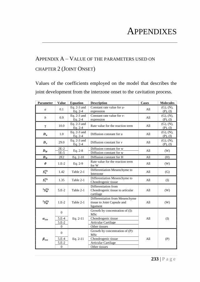
233 | P a g e
APPENDIXES
APPENDIX A – VALUE OF THE PARAMETERS USED ON
CHAPTER 2 (JOINT ONSET)
Values of the coefficients employed on the model that describes the
joint development from the interzone onset to the cavitation process.
Parameter Value Equation Description Cases Molecules
a 0.1 Eq. 2-3 and
Eq. 2-4
Constant rate value for u-
expression All
(G), (N),
(P), (I)
b 0.9 Eq. 2-3 and
Eq. 2-4
Constant rate value for v-
expression All
(G), (N),
(P), (I)
γ 10.0 Eq. 2-3 and
Eq. 2-4 Rate value for the reaction term All
(G), (N),
(P), (I)
𝑫𝒖 1.0 Eq. 2-3 and
Eq. 2-4 Diffusion constant for u All
(G), (N),
(P), (I)
𝑫𝒗 29.0 Eq. 2-3 and
Eq. 2-4 Diffusion constant for v All
(G), (N), (P), (I)
𝑫𝑾 2E-2
Eq. 2-8 Diffusion constant for w
All (W) 5E-5 Diffusion constant for w
𝑫𝑯 2E2 Eq. 2-10 Diffusion constant for H All (H)
𝝑 1.E-2 Eq. 2-9 Rate value for the reaction term
for W All (W)
𝑺𝑮𝑻𝒉 1.42 Table 2-1
Differentiation Mesenchyme to
Interzone All (G)
𝑺𝑰𝑻𝒉 1.35 Table 2-1
Differentiation Mesenchyme to Chondrogenic tissue
All (I)
𝑺𝑾𝑻𝒉𝟏 5.E-2 Table 2-1
Differentiation from Chondrogenic tissue to articular
cartilage
All (W)
𝑺𝑾𝑻𝒉𝟐 1.E-2 Table 2-1
Differentiation from Mesenchyme
tissue to Joint Capsule and ligament
All (W)
𝜶𝒊𝒔𝒐
0
Eq. 2-11
Growth by concentration of (I): MSc
All (I) 5.E-4 Chondrogenic tissue
5.E-2 Articular Cartilage
0 Other tissues
𝜷𝒊𝒔𝒐
0
Eq. 2-11
Growth by concentration of (P):
MSc
All (P) 5.E-4 Chondrogenic tissue
5.E-2 Articular Cartilage
0 Other tissues
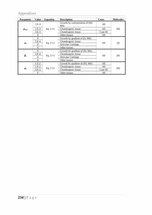
Appendixes
234 | P a g e
Parameter Value Equation Description Cases Molecules
𝝁𝒊𝒔𝒐
1.E-3
Eq. 2-11
Growth by concentration of (H):
MSc All
(H) 1.E-3 Chondrogenic tissue All
3.E-3 Chondrogenic tissue Case III
0 Other tissues All
𝜶𝒊
0
Eq. 2-11
Growth by gradient of (I): MSc
All (I) 5.E-4 Chondrogenic tissue
0 Articular Cartilage
0 Other tissues
𝜷𝒊
0
Eq. 2-11
Growth by gradient of (P): MSc
All (P) 5.E-4 Chondrogenic tissue
0 Articular Cartilage
0 Other tissues
𝝁𝒊
1.E-2
Eq. 2-11
Growth by gradient of (H): MSc All
(H) 1.E-2 Chondrogenic tissue All
3.E-3 Chondrogenic tissue Case III
0 Other tissues All
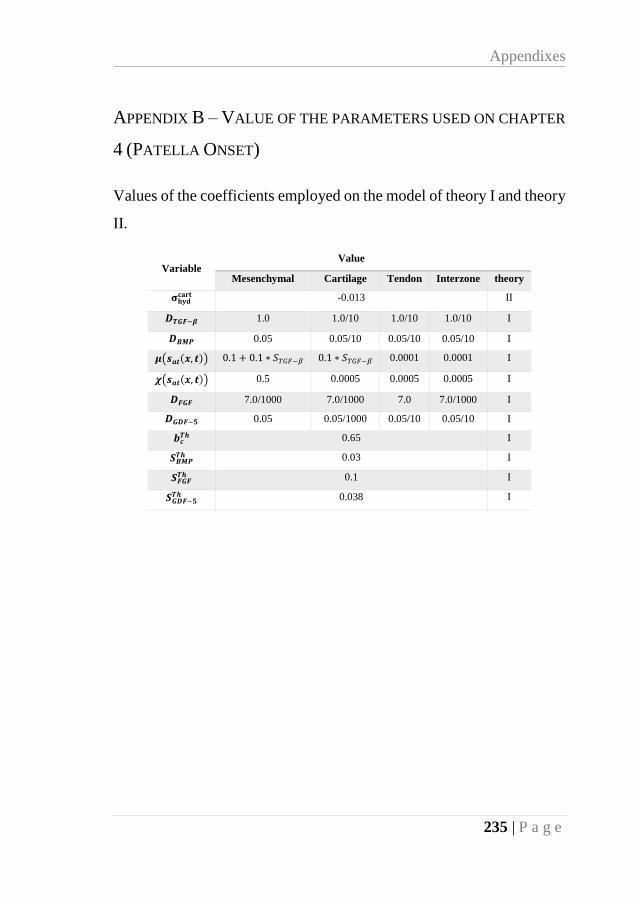
Appendixes
235 | P a g e
APPENDIX B – VALUE OF THE PARAMETERS USED ON CHAPTER
4 (PATELLA ONSET)
Values of the coefficients employed on the model of theory I and theory
II.
Variable Value
Mesenchymal Cartilage Tendon Interzone theory
𝛔𝐡𝐲𝐝𝐜𝐚𝐫𝐭 -0.013 II
𝑫𝑻𝑮𝑭−𝜷 1.0 1.0/10 1.0/10 1.0/10 I
𝑫𝑩𝑴𝑷 0.05 0.05/10 0.05/10 0.05/10 I
𝝁(𝒔𝒂𝒕(𝒙, 𝒕)) 0.1 + 0.1 ∗ 𝑆𝑇𝐺𝐹−𝛽 0.1 ∗ 𝑆𝑇𝐺𝐹−𝛽 0.0001 0.0001 I
𝝌(𝒔𝒂𝒕(𝒙, 𝒕)) 0.5 0.0005 0.0005 0.0005 I
𝑫𝑭𝑮𝑭 7.0/1000 7.0/1000 7.0 7.0/1000 I
𝑫𝑮𝑫𝑭−𝟓 0.05 0.05/1000 0.05/10 0.05/10 I
𝒃𝒄𝑻𝒉 0.65 I
𝑺𝑩𝑴𝑷𝑻𝒉 0.03 I
𝑺𝑭𝑮𝑭𝑻𝒉 0.1 I
𝑺𝑮𝑫𝑭−𝟓𝑻𝒉 0.038 I

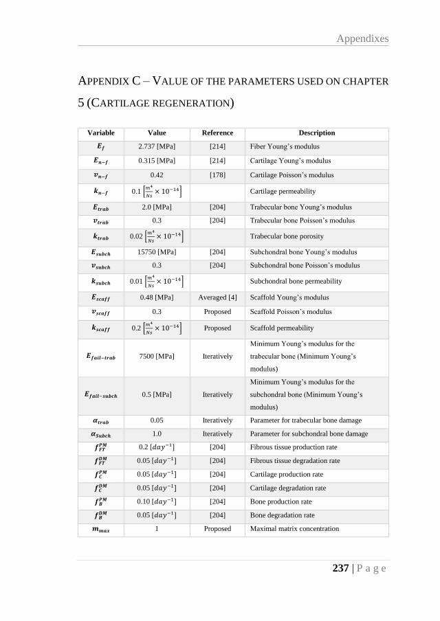
Appendixes
237 | P a g e
APPENDIX C – VALUE OF THE PARAMETERS USED ON CHAPTER
5 (CARTILAGE REGENERATION)
Variable Value Reference Description
𝑬𝒇 2.737 [MPa] [214] Fiber Young’s modulus
𝑬𝒏−𝒇 0.315 [MPa] [214] Cartilage Young’s modulus
𝒗𝒏−𝒇 0.42 [178] Cartilage Poisson’s modulus
𝒌𝒏−𝒇 0.1 [𝑚4
𝑁𝑠× 10−14] Cartilage permeability
𝑬𝒕𝒓𝒂𝒃 2.0 [MPa] [204] Trabecular bone Young’s modulus
𝒗𝒕𝒓𝒂𝒃 0.3 [204] Trabecular bone Poisson’s modulus
𝒌𝒕𝒓𝒂𝒃 0.02 [𝑚4
𝑁𝑠× 10−14] Trabecular bone porosity
𝑬𝒔𝒖𝒃𝒄𝒉 15750 [MPa] [204] Subchondral bone Young’s modulus
𝒗𝒔𝒖𝒃𝒄𝒉 0.3 [204] Subchondral bone Poisson’s modulus
𝒌𝒔𝒖𝒃𝒄𝒉 0.01 [𝑚4
𝑁𝑠× 10−14] Subchondral bone permeability
𝑬𝒔𝒄𝒂𝒇𝒇 0.48 [MPa] Averaged [4] Scaffold Young’s modulus
𝒗𝒔𝒄𝒂𝒇𝒇 0.3 Proposed Scaffold Poisson’s modulus
𝒌𝒔𝒄𝒂𝒇𝒇 0.2 [𝑚4
𝑁𝑠× 10−14] Proposed Scaffold permeability
𝑬𝒇𝒂𝒊𝒍−𝒕𝒓𝒂𝒃 7500 [MPa] Iteratively
Minimum Young’s modulus for the
trabecular bone (Minimum Young’s
modulus)
𝑬𝒇𝒂𝒊𝒍−𝒔𝒖𝒃𝒄𝒉 0.5 [MPa] Iteratively
Minimum Young’s modulus for the
subchondral bone (Minimum Young’s
modulus)
𝜶𝒕𝒓𝒂𝒃 0.05 Iteratively Parameter for trabecular bone damage
𝜶𝑺𝒖𝒃𝒄𝒉 1.0 Iteratively Parameter for subchondral bone damage
𝒇𝑭𝑻𝑷𝑴 0.2 [𝑑𝑎𝑦−1] [204] Fibrous tissue production rate
𝒇𝑭𝑻𝑫𝑴 0.05 [𝑑𝑎𝑦−1] [204] Fibrous tissue degradation rate
𝒇𝑪𝑷𝑴 0.05 [𝑑𝑎𝑦−1] [204] Cartilage production rate
𝒇𝑪𝑫𝑴 0.05 [𝑑𝑎𝑦−1] [204] Cartilage degradation rate
𝒇𝑩𝑷𝑴 0.10 [𝑑𝑎𝑦−1] [204] Bone production rate
𝒇𝑩𝑫𝑴 0.05 [𝑑𝑎𝑦−1] [204] Bone degradation rate
𝒎𝒎𝒂𝒙 1 Proposed Maximal matrix concentration

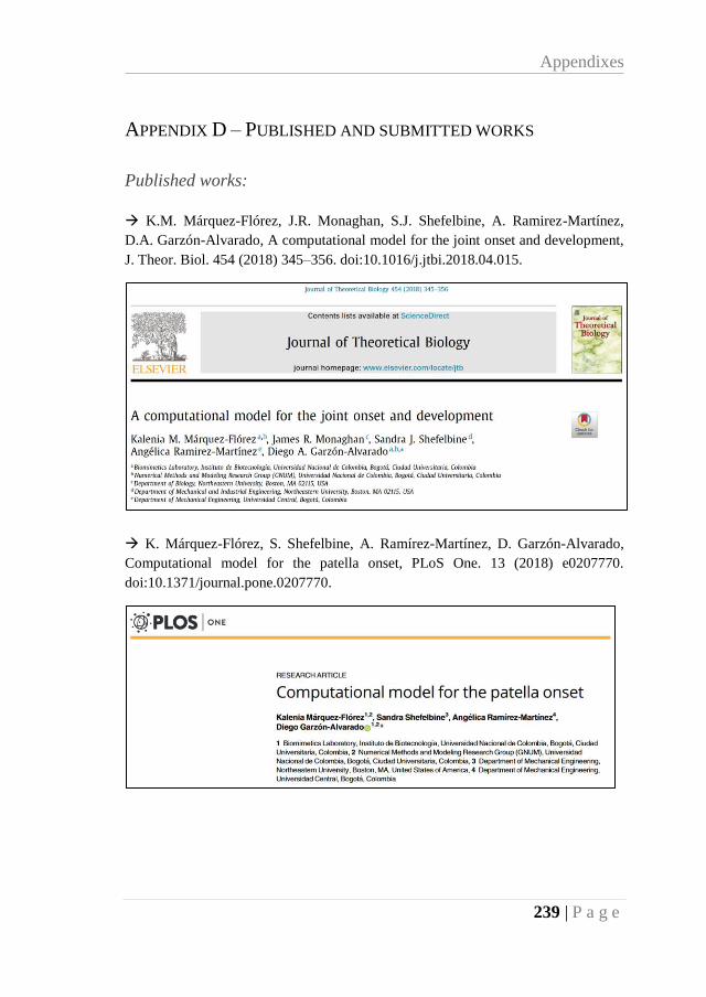
Appendixes
239 | P a g e
APPENDIX D – PUBLISHED AND SUBMITTED WORKS
Published works:
→ K.M. Márquez-Flórez, J.R. Monaghan, S.J. Shefelbine, A. Ramirez-Martínez,
D.A. Garzón-Alvarado, A computational model for the joint onset and development,
J. Theor. Biol. 454 (2018) 345–356. doi:10.1016/j.jtbi.2018.04.015.
→ K. Márquez-Flórez, S. Shefelbine, A. Ramírez-Martínez, D. Garzón-Alvarado,
Computational model for the patella onset, PLoS One. 13 (2018) e0207770.
doi:10.1371/journal.pone.0207770.
Appendixes
240 | P a g e
Submitted works:
Carrera-Pinzón A.F., Márquez-Flórez K., Kraft R., Garzón-Alvarado D.A.,
Computational Model of a Synovial Joint Morphogenesis, PLoS One. 2019- PONE-
S-19-08473
Congresses:
K. Márquez-Flórez, S.J. Shefelbine, D.A. Garzón-Alvarado (June 2017). A
computational approach on patella development. VII International Conference on
Computational Methods for Coupled Problems in Science and Engineering. Coupled
problems 2017, CIMNE. Rhodes, Greece.
Posters:
K. Márquez-Flórez, D. Garzón-Alvarado, C. Carda, M. Sancho-Tello (May
2019). Computational model for the cartilage regeneration process induced by
scaffold implantation. Tissue Engineering and Regenerative Medicine International
Society (TERMIS) EU 2019. Rhodes, Greece.
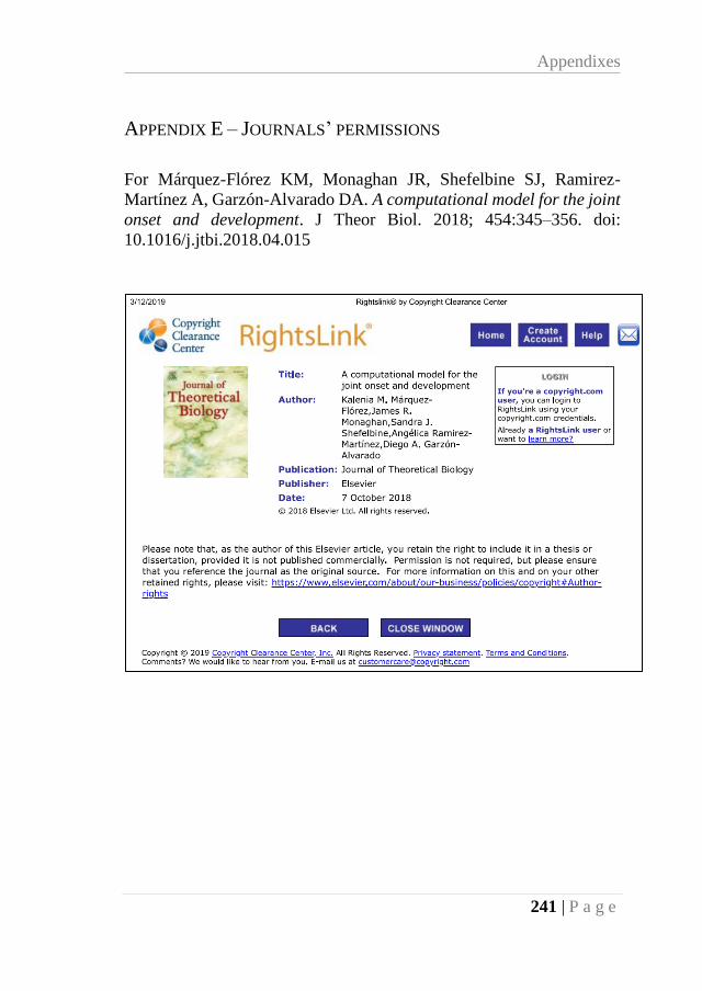
Appendixes
241 | P a g e
APPENDIX E – JOURNALS’ PERMISSIONS
For Márquez-Flórez KM, Monaghan JR, Shefelbine SJ, Ramirez-
Martínez A, Garzón-Alvarado DA. A computational model for the joint
onset and development. J Theor Biol. 2018; 454:345–356. doi:
10.1016/j.jtbi.2018.04.015
Appendixes
242 | P a g e
For Márquez-Flórez K, Shefelbine S, Ramírez-Martínez A, Garzon-
Alvarado DA. Computational model for the patella onset PLoS One.
2018;1–22.
From PLOS webpage: https://journals.plos.org/plosone/s/licenses-and-
copyright
“PLOS applies the Creative Commons
Attribution (CC BY) license to articles and other works
we publish. If you submit your paper for publication by
PLOS, you agree to have the CC BY license applied to
your work. Under this Open Access license, you as the
author agree that anyone can reuse your article in whole
or part for any purpose, for free, even for commercial
purposes. Anyone may copy, distribute, or reuse the
content as long as the author and original source are
properly cited. This facilitates freedom in re-use and
also ensures that PLOS content can be mined without
barriers for the needs of research.”