Embed Size (px)
Citation preview
K. Ensor, STAT 4211
Spring 2004
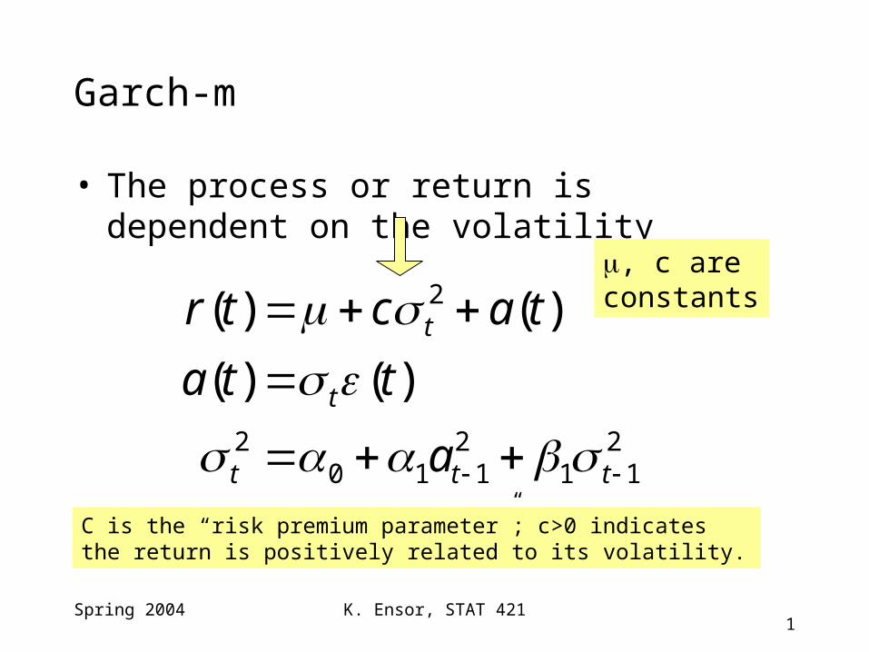
Garch-m
• The process or return is dependent on the volatility
211
2110
2
2
)()(
)()(
ttt
t
t
a
tta
tactr
, c are constants
C is the “risk premium parameter”; c>0 indicates the return is positively related to its volatility.
K. Ensor, STAT 4212
Spring 2004
Time
0 200 400 600 800
-0.2
0.2
Time
0 200 400 600 800
-0.2
0.2
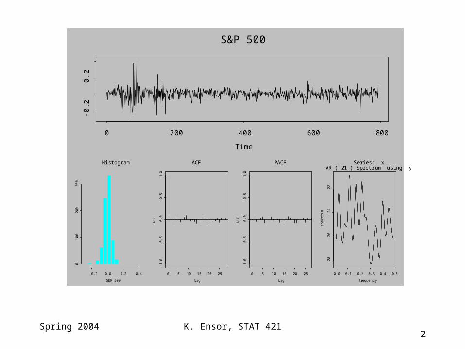
S&P 500
-0.2 0.0 0.2 0.4
01
00
20
03
00
Histogram
S&P 500 Lag
AC
F
0 5 10 15 20 25
-1.0
-0.5
0.0
0.5
1.0
ACF
Lag
AC
F
0 5 10 15 20 25
-1.0
-0.5
0.0
0.5
1.0
PACF
frequency
spe
ctru
m
0.0 0.1 0.2 0.3 0.4 0.5
-28
-26
-24
-22
Series: x AR ( 21 ) Spectrum using yule-walker

K. Ensor, STAT 4213
Spring 2004
Estimated Coefficients:
--------------------------------------------------------------
Value Std.Error t value Pr(>|t|)
C 0.00548675 0.00226173 2.426 7.747e-003
ARCH-IN-MEAN 1.08783589 0.81822755 1.330 9.203e-002
A 0.00008764 0.00002507 3.496 2.494e-004
ARCH(1) 0.12268468 0.02047268 5.993 1.571e-009
GARCH(1) 0.84939373 0.01957565 43.390 0.000e+000
--------------------------------------------------------------
Output from Splus m-garch fitgarch(x~1+var.in.mean,~garch(1,1))
Differs from Tsay’s fit slightly.
K. Ensor, STAT 4214
Spring 2004
-0.2
0.0
0.2
0.4
0 200 400 600 800
Conditional SD
0.05
0.10
0.15
0.20
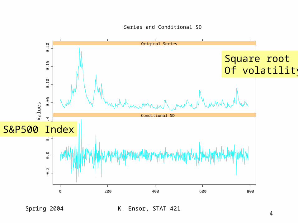
Original SeriesV
alu
es
Series and Conditional SD
S&P500 Index
Square rootOf volatility

K. Ensor, STAT 4215
Spring 2004
0.0
0.2
0.4
0.6
0.8
1.0
0 5 10 15 20 25 30
ACF
Lags
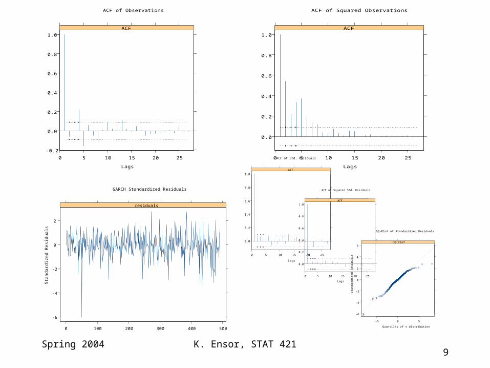
ACF of Squared Observations
0.0
0.2
0.4
0.6
0.8
1.0
0 5 10 15 20 25 30
ACF
Lags
ACF of Observations
-4
-2
0
2
0 200 400 600 800
residuals
Sta
nd
ard
ize
d R
esi
du
als
GARCH Standardized Residuals
0.0
0.2
0.4
0.6
0.8
1.0
0 5 10 15 20 25 30
ACF
Lags
ACF of Std. Residuals
0.0
0.2
0.4
0.6
0.8
1.0
0 5 10 15 20 25 30
ACF
Lags
ACF of Squared Std. Residuals
-4
-2
0
2
-3 -2 -1 0 1 2 3
QQ-Plot
147
173
742
Quantiles of gaussian distribution
Sta
nd
ard
ize
d R
esi
du
als
QQ-Plot of Standardized Residuals
Summary Graphs

K. Ensor, STAT 4216
Spring 2004
-10
-50
510
15
0 100 200 300 400 500
Conditional SD
24
68
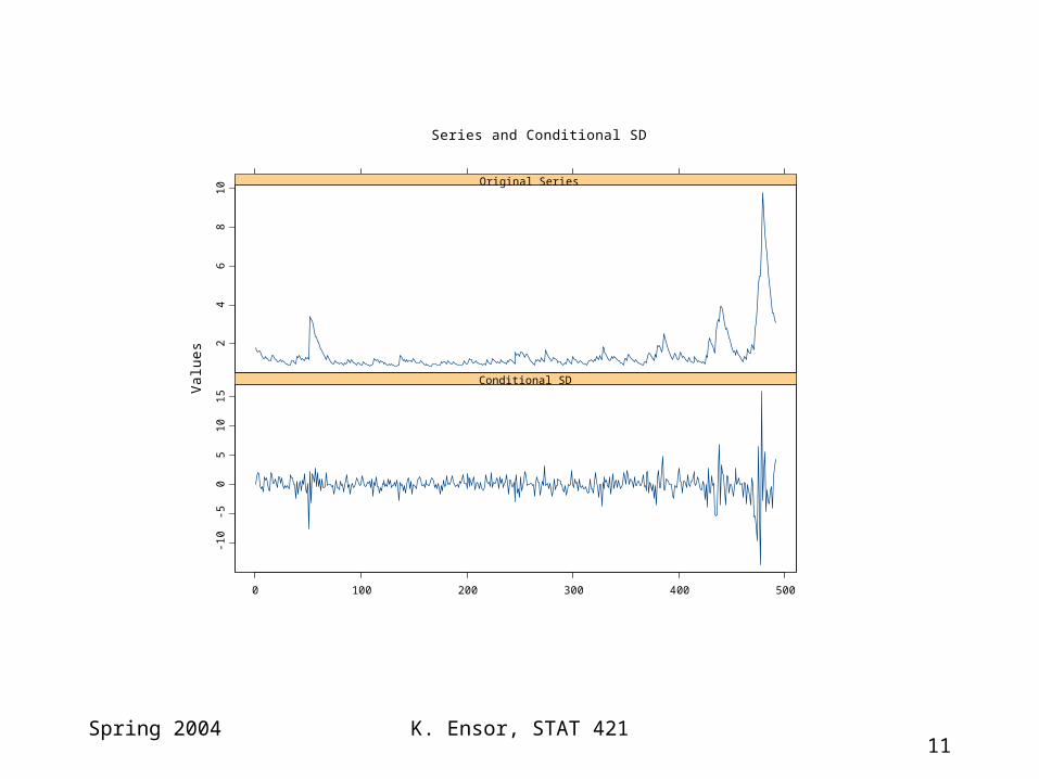
Original Series
Va
lue
s
Series and Conditional SD
Hong Kong stock market index return (bottom graph) and estimated volatility.
K. Ensor, STAT 4217
Spring 2004
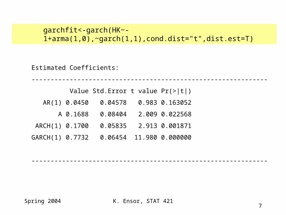
Estimated Coefficients:
--------------------------------------------------------------
Value Std.Error t value Pr(>|t|)
AR(1) 0.0450 0.04578 0.983 0.163052
A 0.1688 0.08404 2.009 0.022568
ARCH(1) 0.1700 0.05835 2.913 0.001871
GARCH(1) 0.7732 0.06454 11.980 0.000000
--------------------------------------------------------------
garchfit<-garch(HK~-1+arma(1,0),~garch(1,1),cond.dist="t",dist.est=T)

K. Ensor, STAT 4218
Spring 2004
-10
0
10
0 100 200 300 400 500
garchfit
Va
lue
s
Series with 2 Conditional SD Superimposed
HK - Garch fit +/- 2SD
K. Ensor, STAT 4219
Spring 2004
-0.2
0.0
0.2
0.4
0.6
0.8
1.0
0 5 10 15 20 25
ACF
Lags
ACF of Observations
0.0
0.2
0.4
0.6
0.8
1.0
0 5 10 15 20 25
ACF
Lags
ACF of Squared Observations
-6
-4
-2
0
2
0 100 200 300 400 500
residuals
Sta
nd
ard
ize
d R
esi
du
als
GARCH Standardized Residuals
0.0
0.2
0.4
0.6
0.8
1.0
0 5 10 15 20 25
ACF
Lags
ACF of Std. Residuals
0.0
0.2
0.4
0.6
0.8
1.0
0 5 10 15 20 25
ACF
Lags
ACF of Squared Std. Residuals
-6
-4
-2
0
2
4
6
-5 0 5
QQ-Plot
32
1
Quantiles of t distribution
Sta
nd
ard
ize
d R
esi
du
als
QQ-Plot of Standardized Residuals

K. Ensor, STAT 42110
Spring 2004
--------------------------------------------------------------
Estimated Coefficients:
--------------------------------------------------------------
Value Std.Error t value Pr(>|t|)
AR(1) 0.1199 0.05709 2.100 1.811e-002
A 0.1424 0.04834 2.946 1.687e-003
ARCH(1) 0.1782 0.03693 4.827 9.287e-007
GARCH(1) 0.7592 0.04913 15.452 0.000e+000
--------------------------------------------------------------
garchfit<-garch(HK~-1+arma(1,0),~garch(1,1),cond.dist="gaussian",dist.est=T)
K. Ensor, STAT 42111
Spring 2004
-10
-50
510
15
0 100 200 300 400 500
Conditional SD
24
68
10
Original Series
Va
lue
s
Series and Conditional SD
K. Ensor, STAT 42112
Spring 2004
-20
-10
0
10
20
0 100 200 300 400 500
garchfit
Va
lue
s
Series with 2 Conditional SD Superimposed

K. Ensor, STAT 42113
Spring 2004
-6
-4
-2
0
2
0 100 200 300 400 500
residuals
Sta
nd
ard
ize
d R
esi
du
als
GARCH Standardized Residuals
-6
-4
-2
0
2
-3 -2 -1 0 1 2 3
QQ-Plot
471434
51
Quantiles of gaussian distribution
Sta
nd
ard
ize
d R
esi
du
als
QQ-Plot of Standardized Residuals

K. Ensor, STAT 42114
Spring 2004
-10
-50
510
15
0 100 200 300 400 500
Conditional SD
24
68
Original Series
Va
lue
s
Series and Conditional SD
Japanese stock market index and volatility based on Gaussian GARCH(1,1) model
K. Ensor, STAT 42115
Spring 2004
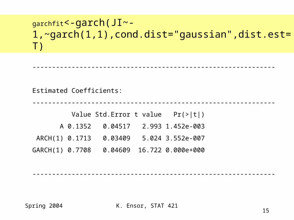
--------------------------------------------------------------
Estimated Coefficients:
--------------------------------------------------------------
Value Std.Error t value Pr(>|t|)
A 0.1352 0.04517 2.993 1.452e-003
ARCH(1) 0.1713 0.03409 5.024 3.552e-007
GARCH(1) 0.7708 0.04609 16.722 0.000e+000
--------------------------------------------------------------
garchfit<-garch(JI~-1,~garch(1,1),cond.dist="gaussian",dist.est=T)

K. Ensor, STAT 42116
Spring 2004
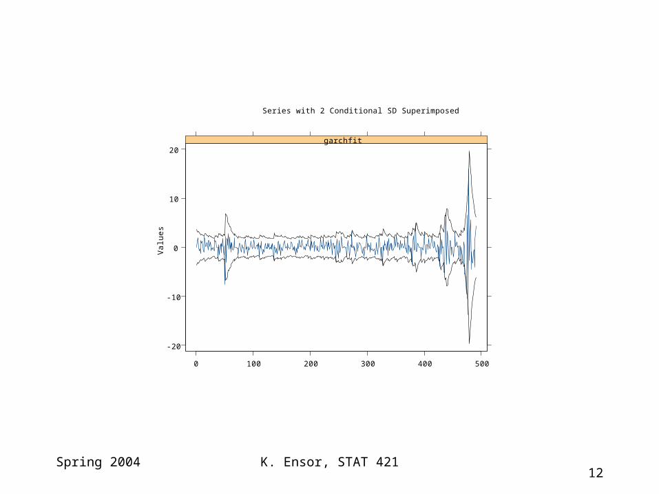
-20
-10
0
10
20
0 100 200 300 400 500
garchfitV
alu
es
Series with 2 Conditional SD Superimposed
JI
K. Ensor, STAT 42117
Spring 2004
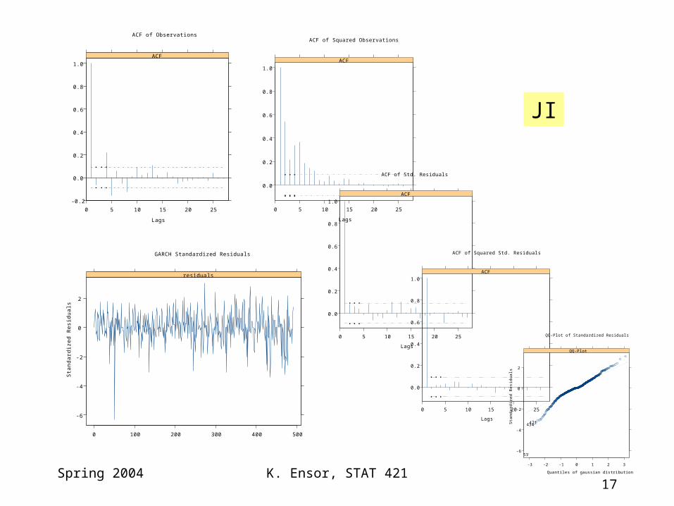
-0.2
0.0
0.2
0.4
0.6
0.8
1.0
0 5 10 15 20 25
ACF
Lags
ACF of Observations
0.0
0.2
0.4
0.6
0.8
1.0
0 5 10 15 20 25
ACF
Lags
ACF of Squared Observations
-6
-4
-2
0
2
0 100 200 300 400 500
residuals
Sta
nd
ard
ize
d R
esi
du
als
GARCH Standardized Residuals
0.0
0.2
0.4
0.6
0.8
1.0
0 5 10 15 20 25
ACF
Lags
ACF of Std. Residuals
0.0
0.2
0.4
0.6
0.8
1.0
0 5 10 15 20 25
ACF
Lags
ACF of Squared Std. Residuals
-6
-4
-2
0
2
-3 -2 -1 0 1 2 3
QQ-Plot
471434
51
Quantiles of gaussian distribution
Sta
nd
ard
ize
d R
esi
du
als
QQ-Plot of Standardized Residuals
JI
K. Ensor, STAT 42118
Spring 2004
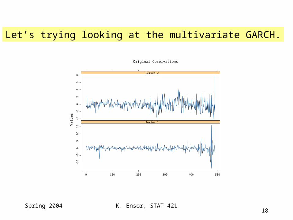
-10
-50
510
15
0 100 200 300 400 500
Series 1
-4-2
02
46
8
Series 2V
alu
es
Original Observations
Let’s trying looking at the multivariate GARCH.

K. Ensor, STAT 42119
Spring 2004
Series 1: Hong Kong Stock IndexSeries 2: Japanese Stock Index
Series 1 A
CF
0 5 10 15 20 25
-0.2
0.0
0.2
0.4
0.6
0.8
1.0
Series 1 and Series 2
0 5 10 15 20 25
-0.1
0.0
0.1
0.2
0.3
Series 2 and Series 1
Lag
AC
F
-25 -20 -15 -10 -5 0
-0.1
0.0
0.1
0.2
0.3
Series 2
Lag0 5 10 15 20 25
0.0
0.2
0.4
0.6
0.8
1.0
ACF of Observations

K. Ensor, STAT 42120
Spring 2004
Series 1 A
CF
0 5 10 15 20
0.0
0.2
0.4
0.6
0.8
1.0
Series 1 and Series 2
0 5 10 15 20
-0.0
50
.00
.05
0.1
00
.15
Series 2 and Series 1
Lag
AC
F
-20 -15 -10 -5 0
0.0
0.2
0.4
0.6
Series 2
Lag0 5 10 15 20
0.0
0.2
0.4
0.6
0.8
1.0
Multivariate Series : X
Series 1: Hong Kong Stock Index SquaredSeries 2: Japanese Stock Index Squared
K. Ensor, STAT 42121
Spring 2004
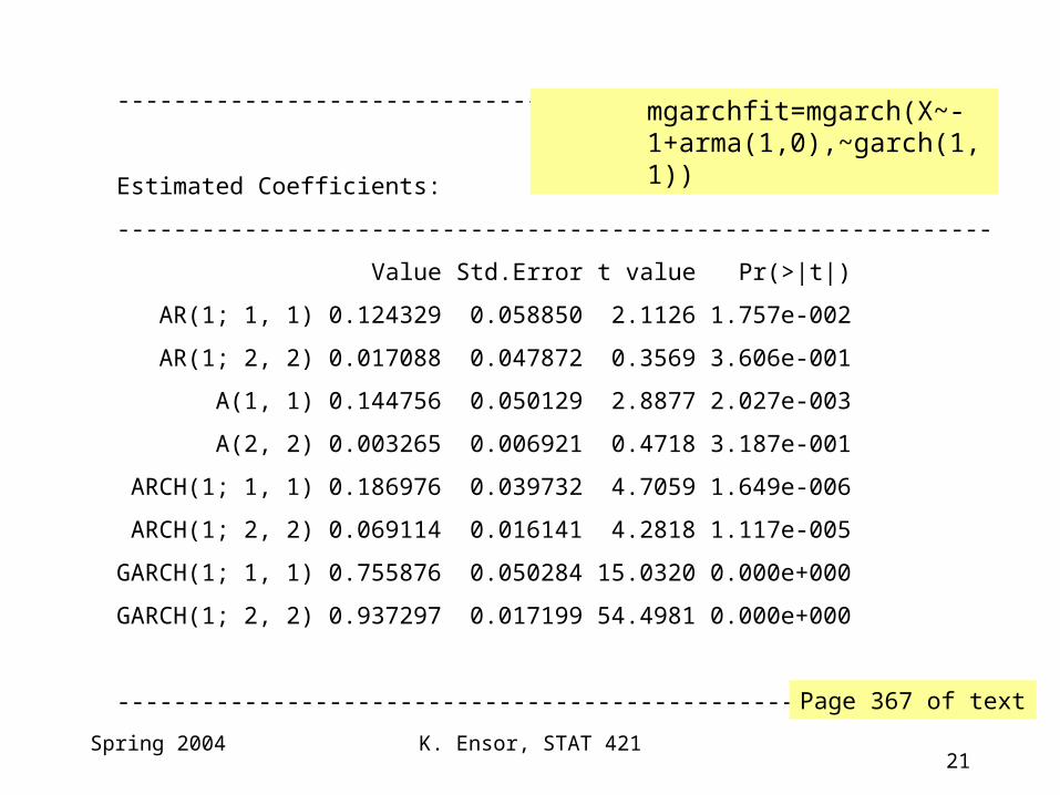
--------------------------------------------------------------
Estimated Coefficients:
--------------------------------------------------------------
Value Std.Error t value Pr(>|t|)
AR(1; 1, 1) 0.124329 0.058850 2.1126 1.757e-002
AR(1; 2, 2) 0.017088 0.047872 0.3569 3.606e-001
A(1, 1) 0.144756 0.050129 2.8877 2.027e-003
A(2, 2) 0.003265 0.006921 0.4718 3.187e-001
ARCH(1; 1, 1) 0.186976 0.039732 4.7059 1.649e-006
ARCH(1; 2, 2) 0.069114 0.016141 4.2818 1.117e-005
GARCH(1; 1, 1) 0.755876 0.050284 15.0320 0.000e+000
GARCH(1; 2, 2) 0.937297 0.017199 54.4981 0.000e+000
--------------------------------------------------------------
mgarchfit=mgarch(X~-1+arma(1,0),~garch(1,1))
Page 367 of text
K. Ensor, STAT 42122
Spring 2004
-10
-50
510
15
0 100 200 300 400 500
Series 1
-4-2
02
46
8
Series 2
Re
sid
ua
ls
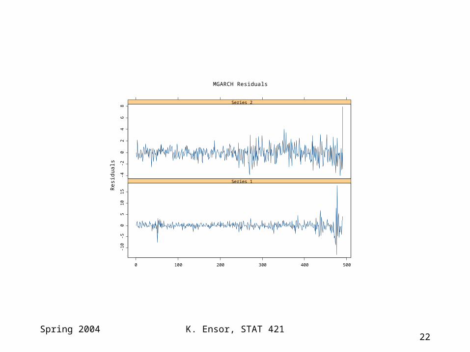
MGARCH Residuals
K. Ensor, STAT 42123
Spring 2004
24
68
10
0 100 200 300 400 500
Series 10.6
1.0
1.4
1.8
Series 2
Co
nd
itio
na
l SD
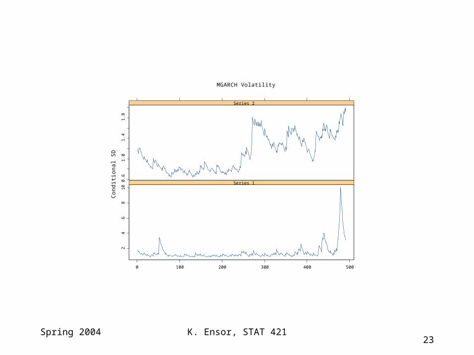
MGARCH Volatility
K. Ensor, STAT 42124
Spring 2004
-6-4
-20
2
0 100 200 300 400 500
Series 1
-20
24
Series 2
Sta
nd
ard
ize
d R
esi
du
als
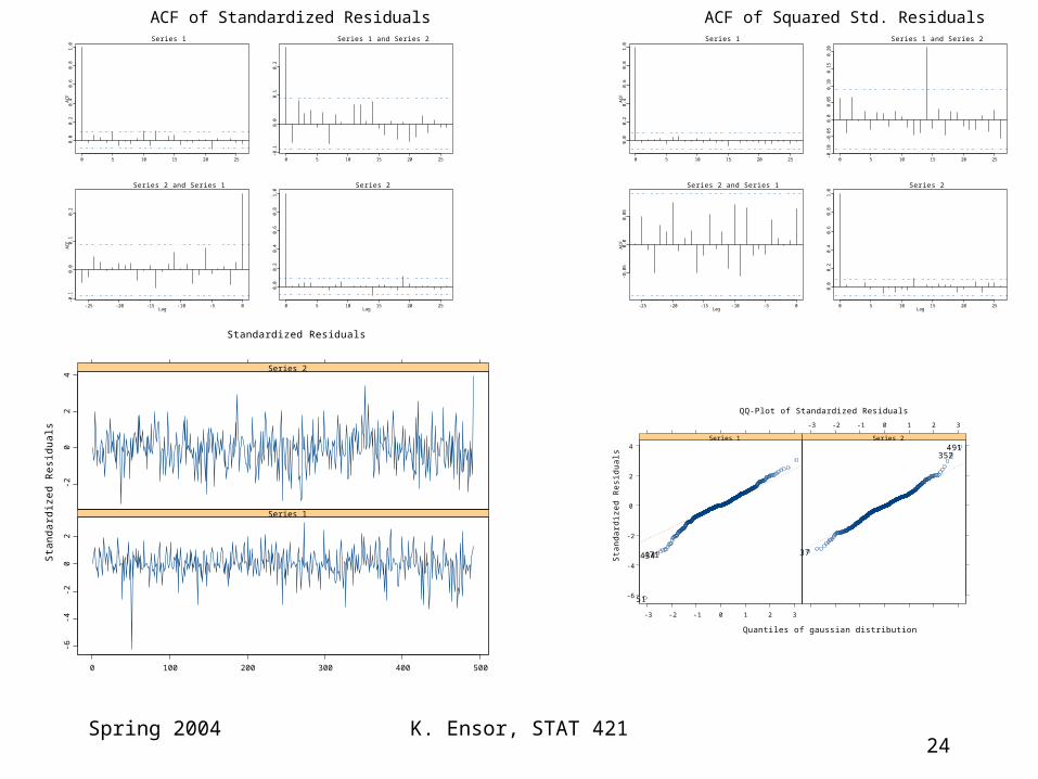
Standardized Residuals
Series 1
AC
F
0 5 10 15 20 25
0.0
0.2
0.4
0.6
0.8
1.0
Series 1 and Series 2
0 5 10 15 20 25
-0.1
0.0
0.1
0.2
Series 2 and Series 1
Lag
AC
F
-25 -20 -15 -10 -5 0
-0.1
0.0
0.1
0.2
Series 2
Lag0 5 10 15 20 25
0.0
0.2
0.4
0.6
0.8
1.0
ACF of Standardized Residuals Series 1
AC
F
0 5 10 15 20 25
0.0
0.2
0.4
0.6
0.8
1.0
Series 1 and Series 2
0 5 10 15 20 25
-0.1
0-0
.05
0.0
0.0
50
.10
0.1
50
.20
Series 2 and Series 1
Lag
AC
F
-25 -20 -15 -10 -5 0
-0.0
50
.00
.05
Series 2
Lag0 5 10 15 20 25
0.0
0.2
0.4
0.6
0.8
1.0
ACF of Squared Std. Residuals
-6
-4
-2
0
2
4
-3 -2 -1 0 1 2 3
Series 1
471434
51
-3 -2 -1 0 1 2 3
Series 2
37
352491
Quantiles of gaussian distribution
Sta
nd
ard
ize
d R
esi
du
als
QQ-Plot of Standardized Residuals