PAPER #5DISCUSSION

June 2016

Assessment of the Comparative Productive Performance of Three Solar PV Technologies Installed at UQ Gatton Campus Using the NREL SAM Model

Prepared by Phillip Wild, PhDPostdoctoral Research Fellow

Global Change InstituteThe University of Queensland

1

Assessment of the Comparative Productive Performance of Three Solar PV Technologies Installed at UQ Gatton Campus Using The NREL SAM Model

By Phillip Wild Email: p.wild@uq.edu.au

Telephone: work (07) 3346 1004; Mobile 0412 443 523 Version 4 – 15 June 2016

Abstract

The economic assessment of the viability of different types of solar PV tracking

technologies centres on assessment of whether the annual production of the different tracking

technologies is increased enough to compensate for the higher cost of installation and

operational expenditures incurred by the tracking systems. To investigate this issue, we use

the NREL’s SAM model to simulate electricity production from three representative solar PV

systems installed at Gatton. In these simulations we use hourly solar irradiance, weather and

surface albedo data, technical data relating to both module and inverter characteristics and

impacts associated with module soiling and near-object shading. A key finding was that over

the period 2007 to 2015, average increases in annual production of between 23.9 and 24.3 per

cent and 38.0 and 39.1 per cent were obtained for Single Axis and Dual Axis tracking

systems relative to the Fixed Tilt system.

(1) Introduction

The economics of solar PV has changed significantly over the last decade with

installation costs declining significantly following the marked take-up of solar PV systems,

often on the back of generous Government feed-in tariff support particularly in Europe.

More recently, a marked increase in the up-take of roof-top solar PV occurred in Australia on

the back of generous state-based Feed-in tariffs and the Federal Government’s renewable

energy target, and, more recently, the small scale renewable energy target (RMI, 2014).

2

Unlike the case in particularly Spain and Germany, however, there were no equivalent feed-

in tariffs available for large scale investments in Australia, and these types of investments

have been much slower to emerge.

To-date, investment in large commercial and industrial scale solar PV projects has

largely proceeded on the basis of support from two particular programs: (1) Australian

Capital Territory (ACT) reverse auction for solar PV projects (ACT, 2016); and (2)

Government support from the Australian Renewable Energy Agency (ARENA, 2016), in

conjunction with financial support from the Clean Energy Finance Corporation (CEFC) for

larger projects (CEFC, 2016). This has occurred against a general backdrop of a concerted

attack on renewable energy in Australia since late 2013. Moreover, policy and regulatory

uncertainty accompanying this attack has led to a general drying up of investment in large-

scale renewable energy projects with major retail electricity companies now appearing

unwilling to enter Power Purchase Agreement (PPA) agreements traditionally needed to

secure private sector finance for projects. This has led to the situation whereby the required

capacity to meet the 2017 Large Scale Renewable Energy Target (LRET) now appears to be

in excess of 3000 MW’s in arrears (Green Energy Markets, 2015).

The structure of this paper is as follows. The next section will give a brief description

of the solar array at the University of Queensland’s (UQ) Gatton Campus that underpins the

modelling performed for this paper. Section (3) will contain a discussion of critical aspects

affecting the comparative assessment of the production of representative technologies

contained in the solar array under investigation. This will include an outline the modelling

employed in the paper to generate solar PV yield and discussion of the results of the

modelling relating to production and annual capacity factor (ACF) outcomes, respectively.

Section 4 will contain conclusions.

(2) University of Queensland Gatton Solar Research Facility (GSRF)

The GSRF was funded under the Federal Government’s Education Investment Fund (EIF)

scheme ($40.7M), and was part of the larger ARENA funded project Australian Gas and Light Pty

Ltd (AGL) Nyngan and Broken Hill Solar farms (UQ, 2015a). These two solar PV farms have a

capacity of 102 MW and 53 MW, respectively. The total cost of the combined project was

$439.08 million, of which ARENA contributed $166.7 million and the New South Wales

3

State Government $64.9 million (AGL, 2015). The objective of the EIF Project was to act as a

pilot for the utility-scale plants – proofing technology and establishing supply chains.

The GSRF solar array installed at Gatton is a 3.275 megawatt pilot plant that

comprises three different solar array technologies: (1) a Fixed Tilt (FT) array comprising

three identical 630 kW systems (UQ, 2015b); (2) a 630 kW Horizontal Single Axis Tracking

(SAT) Array utilising First Solar’s SAT system (UQ, 2015c); and (3) a 630 kW Dual Axis

Tracker (DAT) utilising the Degertraker 5000 HD system (UQ, 2015d). A good overview of

the principals underpinning sun-tracking methods can be found in Mousazadeh et al. (2009).

An overhead NearMap picture of the Gatton array is contained in Figure 1. The FT

system design at Gatton has the following technical design features: (1) all modules have a

tilt angle of 20 degrees; (2) all modules have an azimuth angle of 357 degrees (e.g. modules

are facing in the direction of three degrees west of north). The three FT arrays have a

combined total of 21, 600 modules. These arrays can be located, respectively, at the top right

hand side (termed the ‘top’ FT array) and with the main FT array being located just below the

buildings and line of trees but above the road in Figure 1.

The SAT array at Gatton has the following technical aspects: (1) the array is a

horizontal array and thus has a tilt angle of 0 degrees; (2) the array has an azimuth angle of

357 degrees (e.g. same as the FT system); (3) maximum tracker rotation limit is set to 45

degrees; and (4) no backtracking is implemented. Backtracking is a control procedure that is

used in some SAT systems to minimise the degree of self-shading from nearby SAT trackers.

The total number of modules in the SAT array is 7,200 modules with 120 individual SAT

tracking systems. The SAT array can be located in Figure 1 immediately below the top FT

array, adjacent to the main FT array and also above the road in Figure 1.

The third array is the DAT array. There are 160 individual trackers installed at Gatton

that are capable of a 340 degree slewing motion and a 180 degree tilt that allow the modules

to directly face the sun at all times of the day, thereby maximising output (UQ 2015d). As in

the case of the SAT system, the DAT system also has 7,200 modules in total. In Figure 1, the

DAT array is located underneath the main FT array and below the road.

Figure 1. NearMap Picture of the UQ Gatton Solar Array

4

The same type of modules are installed on all three solar array technologies located at

Gatton – First Solar FS-395 PLUS (95 W) modules. The same type of inverter is also

installed with each of the 630 kW systems – SMA Sunny Central 720CP XT inverters. The

three FT sub-arrays are connected to three inverters while the SAT and DAT sub-arrays are

connected to a single inverter each. Hence, the whole array contains five inverters.

Moreover, through the connection agreement with Energex, each inverter’s output is

currently limited to 630 kW.

In this paper we will restrict attention to a comparative assessment of the production

results of three representative 630 kW FT, SAT and DAT sub-arrays. This will involve

assessing the output performance of the SAT and DAT sub-arrays and the left hand side sub-

array of the main FT array installed at Gatton – e.g. the left most FT sub-array.

(3) Comparative Assessment of Production Outcomes of the Three

Representative Arrays at Gatton.

Economic assessment of the viability of different types of solar PV tracking

technologies typically centres on an assessment of whether the annual production of the

different tracking technologies is lifted enough relative to the benchmark FT system in order

to compensate for the higher installation and operational costs incurred by the tracking

systems. The installation costs refer to the ‘overnight’ ($/Wp) or equivalently ($/kW)

installation costs that would be incurred if the whole solar PV plant could be constructed

overnight. This expenditure category would include costs associated with the purchase of

5

modules and inverters as well as various categories of balance of plant costs. The latter

component would include expenditures associated with: (1) costs of transport to site; (2) site

preparation, racking and mounting activities; (3) DC and AC electrical connection; and (4)

other non-production activity such as insurance costs, administration and connection

licensing (RMI, 2014).

The second cost component is operational costs, in particular, Operational and

Maintenance (O&M) expenditures associated with keeping modules and inverters operating

efficiently. For tracking systems, additional O&M costs would also have to be levied against

the need to also keep the tracking infrastructure working efficiently. In general, solar tracking

systems include a tracking device, tracking algorithm, control unit, positioning system,

driving mechanism and sensing devices.

Large optical errors in tracking the sun’s position will result in potentially large

reductions in electricity generated from the PV system relative to what would have been

obtained if the tracking mechanism was working properly. A crucial question, however, is

how large is how large? Mousazadeh et al. (2009) point out that trackers do not need to be

pointed directly at the sun to be effective. They argued that if the aim is off by 10 degrees

implying an optical tracking error of 10 degrees, the output will still be 98.5% of the full-

tracking maximum. Stafford et al. (2009) report that tracking errors may not be negligible

when compared with typical system acceptance angles – the maximum pointing error that the

PV system can tolerate without a substantial loss of power output. They also found that the

fraction of available energy captured tended to decline with the degree of the system’s

acceptance angle, whilst increasing with the degree of the acceptance angle. Additional

support for this broad finding is also cited in (Sallaberry et al, 2015a, p. 195). However,

complicating this issue is the observation in Stafford et al (2009) that different solar

technologies such as High Concentration Photovoltaic (HCPV), Low Concentration

Photovoltaic (LCPV), Concentrated Solar Thermal (CSP) and single- and dual-axis tracked

flat-plate PV panels all have different relationships between generated power and tracking

error, leading to different tracking requirements for each technology.

If large reductions in output arise because of the presence of large optical tracking

errors relative to the system’s acceptance angle, this would impair the economic viability of

the tracking system. Some electricity must also be consumed internally by the system in order

to operate the motors that drive the shifts in position of one or more of the axes associated

6

with the particular tracking mechanism. This internal electricity consumption is typically

netted of the gross output produced by the system when tracking is operating during the day.

Thus, O&M expenses are likely to be directly proportional to the complexity of the

tracking system employed. As such, O&M provisions associated with more complex two axis

trackers such as the DAT system are likely to be of a higher magnitude because the tracking

infrastructure is more complex and larger in scale and is, therefore, more likely to be prone

to mechanical faults or break-downs.

(3.1) Assessment of System Output Using National Renewable Energy

Laboratory (NREL) System Advisor Model (SAM)

The SAM model, developed by NREL, was used to simulate electricity production of

the three representative solar PV systems installed at Gatton. To run simulations in SAM,

various user supplied inputs are required. These relate to: (1) hourly solar and weather data;

(2) technical information about modules, inverters and array sizing and design; (3) soiling

effects; (4) shading effects; and (5) DC and AC electrical losses. In the modelling performed

for this paper, we also assumed that all modules, inverters and tracking infrastructure were in

good working order throughout the SAM simulations.

Solar and weather data

The solar and weather data are stored in a SAM CSV weather file which contains

information on the solar PV site’s latitude, longitude, elevation and time zone (Gilman, 2015,

Ch. 3). The solar data included in the file relates to Global Horizontal Irradiance (GHI),

Direct Normal Irradiance (DNI) and Diffuse Horizontal Irradiance (DHI). There is an option

in SAM for the software to internally calculate DHI using internal calculations of the sun’s

position by the software given the latitude, longitude, elevation of the site and commencing

date and time of the simulation. This option was utilised in the simulations underpinning the

results reported in this paper. The Perez Sky Diffuse model is also used to determine Plane-

of-Array (POA) irradiance (Gilman, 2015, Section 6.2).

The GHI and DNI data used in the simulations were obtained from the Australian

Bureau of Meteorology’s (BOM) hourly solar irradiance gridded data (BOM, 2015). The

actual DHI data included in the SAM CSV weather files were calculated from the following

equation:

7

,__cos anglezenithsunDNIGHIDHI (1)

after determining the sun’s position and zenith angle according to the algorithm in Reda and

Andreas (2003). However, recall that the SAM model calculates the sun’s position internally

and the actual DHI data used in the simulations was also calculated internally by SAM, over-

writing the DHI data included originally in the weather file.

The climate data required by the SAM model included both ambient and dew point

temperature (degrees Celsius), relative humidity (percentage), mean sea level pressure

(MSLP in hectopascals), wind speed (meters per second) and wind direction (degree east of

north). This data was sourced from the BOM’s Automatic Weather Station (AWS) located at

the University of Queensland campus at Gatton. This data was supplemented by MSLP

pressure data from the BOM’s Amberley and Toowoomba weather stations because they

were not available for Gatton. Gatton pressure was calculated by the relation:

,__105075.0__ MSLPToowoombaMSLPAmberleyMSLPToowoombaMSLPGatton

(2)

with the coefficient ‘0.105075’ reflecting the fact that pressure changes with elevation. Thus

we include an additional adjustment to the Amberley MSLP value to reflect the fact that

Gatton has a higher elevation than Amberley but is much closer in elevation to Amberley

than to Toowoomba. For example, Gatton has an elevation of 89 meters, Amberley 24.2

meters and Toowoomba 640.9 meters. Given these elevation levels, the coefficient

‘0.105075’ used in equation (2) was calculated as the ratio of the difference in elevation

between Gatton and Amberley and the difference in elevation between Toowoomba and

Amberley, that is, as (89-24.2)/(640.9-24.2).

It should also be noted that only the ambient temperature and wind speed data are

actually used by SAM in modelling solar PV yield. However, the SAM model requires the

other data to be included in the weather file otherwise the program will not run. Finally, we

also include in the SAM CSV weather file data for snow cover (set to zero) and surface

albedo. The surface albedo data was compiled from MODIS White Sky Albedo data (NASA,

2015). This was taken from representative two weekly samples taken at the Gatton latitude

and longitude coordinates to reflect differences in both season and ENSO cycle status.

Specifically, averages of MODIS white albedo readings were obtained for the list of dates in

Table 1.

8

Table1. Dates used to estimate surface albedo at Gatton by season

and ENSO Status

Season La Nina ENSO Neutral El Nino

Summer 9-24 January 2009 11-26 December

2013

10-26 December

2009

Autumn 7-22 April 2010 7-22 April 2013 7-22 April 2006

Winter 2-17 June 2010 10-25 June 2013 10-25 June 2006

Spring 8-23 October 2010 16-31 October 2013 16-31 October 2009

Module, inverter and solar array design

Data is also required about the technical characteristics of the modules and inverters

used at Gatton. As mentioned above, the modules used are First Solar FS-395 PLUS (95 W)

modules while the inverters are SMA Sunny Central 720CP XT inverters. Sets of technical

parameters from First Solar and SMA’s product data sheets for the modules and inverters

were required for the specific module and inverter models used in the SAM modelling. In the

case of the modules, the model used in the SAM simulations was the ‘California Energy

Commission (CEC) Performance Model with User Entered Specifications’ option (Gilman,

2015, Ch. 9.5). The technical parameters required by this model and the values used in the

SAM simulations are listed in Appendix A, Panel (A). This option makes use of a coefficient

calculator developed in Dobos (2012) to calculate the model parameters required by the CEC

model from standard module specifications provided on manufacturer’s data sheets. This

model also uses the NOCT cell temperature model to model cell temperatures (Gilman, 2015,

Ch. 9.7).

The option used to model the inverter was the ‘Inverter Datasheet’ implementation of

the Sandia Inverter Model (Gilman, 2015, Ch. 11.2) with the technical parameters and the

values used in the SAM simulations listed in Appendix A, Panel (B). Recall that for each of

the three FT, SAT and DAT systems modelled, 7200 modules and a single inverter was used,

with the inverter’s AC output constrained to 630 kWac in each case.

9

Implementation of SAM modelling also required data relating to system design

features. In the design and sizing of the array, the most crucial information is: (1) number of

modules in a string; (2) number of strings in parallel; and (3) number of inverters. From this

information as well as from the additional information relating to both modules and inverters,

the following system information is determined: (1) maximum DC capacity of the solar array;

(2) maximum DC input capacity of the inverters; and (3) maximum AC output capacity of the

inverters. The key system design parameters and quantities used in the SAM simulations are

reported in Panel © of Appendix A.

Soiling effects

In order to calculate the various system-wide capacity limits and running simulations

in SAM, account needs to be taken of module soiling (Gilman, 2015, Ch. 7.5). It is generally

accepted that after solar irradiance and air temperature, module soiling will be the next most

crucial issue affecting solar PV yield. Four different soiling rate assumptions were employed

in the modelling for the paper. These relate to low, medium and high soiling scenarios and

additionally, a soiling scenario based upon recommendations of First Solar (ARUP, 2015).

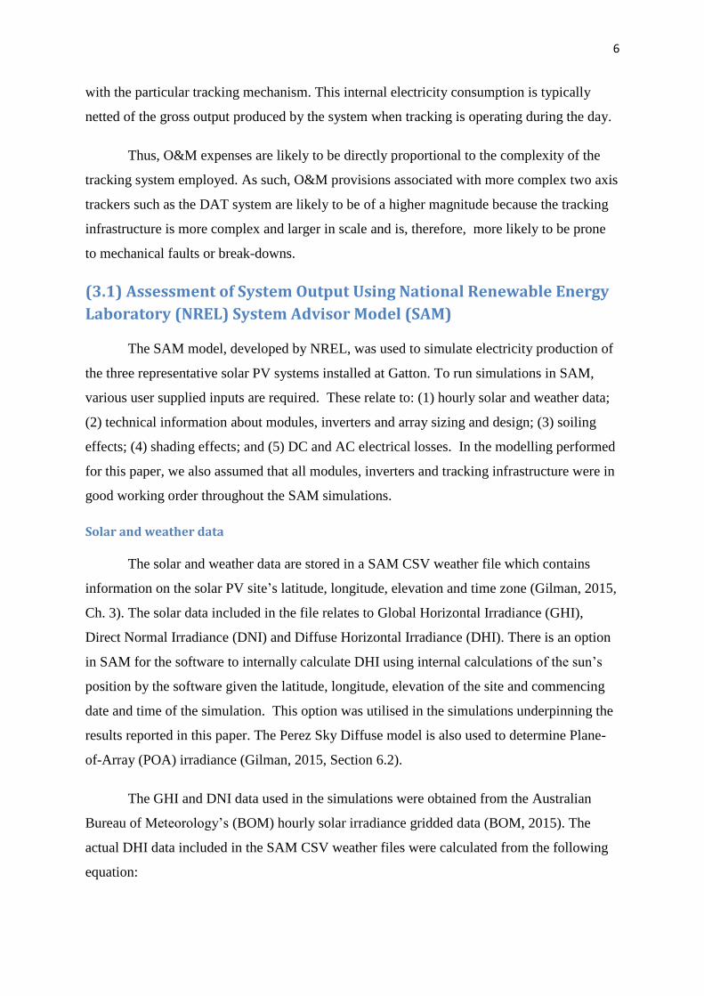
All soiling scenarios are based upon consideration of recorded daily rainfall over the

period 2007 to 2015. The rainfall data utilised in constructing the various soiling scenarios is

that recorded at the UQ Gatton Campus BOM AWS located within two kilometres of the

solar farm. The mean average monthly rainfall for this site is presented in Figure 2. This

figure clearly shows a wet season encompassing the period November to March and a dry

season arising over the period April to September with a transition period between these two

seasons occurring in October.

In determining monthly soiling rates, it was assumed that 25 millimetres (mm) or

more of rainfall during a particular day in a month would be sufficient to restore the modules

to their ‘pristine’ condition associated with their commissioning. During the wet season, it

was common to have some days with a couple of inches of rainfall and multiple days with

over an inch of rainfall. Similarly, it was assumed that daily rainfall totals of less than 5 mm

was not sufficient to engender any cleansing of the modules. Relatively small amounts of

cleaning were assumed for daily rainfall totals of between 5 mm and 10 mm, relating to

reduced accumulative soiling within a month of 20%. More moderate cleansing power for

daily rainfall totals of between 10 mm and 16 mm were assumed that reduced accumulated

10

soiling within a month by 50%. Finally, for daily rainfall totals between 17 mm and 25 mm, it

was assumed that accumulated soiling within a month was reduced by 80%.

Figure 2. Mean average rainfall at UQ Gatton Campus BOM AWS

The accumulative soiling was calculated from the monthly rainfall totals recorded for

the UQ Gatton Campus BOM AWS for two different daily soiling rates assumptions

associated with daily rainfall totals within each month that was less than or equal to 5 mm.

The low soiling scenario assumed a daily growth in soiling effect of 0.033% per day. The

medium soiling scenario assumed a higher daily soiling rate of 0.11% per day. It should be

noted that the daily soiling rate of 0.11% per day was adopted from (Kimber et al, 2006) who

estimated this daily soiling rate for rural areas in Central Valley and Northern California – for

example, see Figure 3 of (Kimber et al, 2006). Assuming a 30 day month, these two daily

soiling rates would produce monthly soiling rates of 1.0 and 3.3 per cent, respectively. To the

extent that consecutive months had no rainfall (defined as less than or equal to 5 mm per

day), these monthly soiling rates would be added together over time producing monthly

soiling rates that could significantly exceed 1.0 and 3.3 per cent.

11

If daily rainfall exceeded 25 mm during the month, total module cleansing was

assumed with the monthly soiling rate being set back to the assumed ‘pristine’

commissioning rate of 1.0 per cent. If one or more of the daily rainfall totals during the

month was between 5 mm and 10 mm, 80 per cent of the assumed within month soiling rate

was added on to the previous months soiling rate thus indicating some marginal cleansing

effect on the modules. If one or more of the daily rainfall totals was between 10 mm and 16

mm, 50 per cent of the assumed within monthly soiling rate was added onto the previous

months soiling rate, indicating some partial cleansing effect on the modules. If one or more of

the daily rainfall totals fell between 17 mm and 25 mm, only 20 per cent of the assumed

within monthly soiling rate was added onto the previous months soiling rate. Thus the main

effect of daily rainfall less than 25 mm is to offset some of the accumulated within month

soiling effect with the larger impacts being associated with daily rainfall rates of between 17

mm and 25 mm.

For completeness, a fourth soiling scenario is also employed, based on an approach

recommended by First Solar (ARUP, 2015, Section 4.2.1.3). This approach involves

assuming a monthly soiling rate of 3.0 per cent if monthly rainfall was less than 20 mm, 2.0

per cent if monthly rainfall was between 20 mm and 50 mm and 1.0 per cent if the monthly

rainfall was greater than 50 mm.

The monthly soiling rates were also corrected for local spectrum following the

method advocated in First Solar (2015). This correction is based upon the fact that modules

are rated under Standard Test Conditions assuming a spectral distribution as defined by

ASTM G173 for an air mass of 1.5. However, site-specific spectral irradiance will typically

deviate from STC resulting in varying performance in regard to module nameplate capacity.

First Solar proposed a method to account for that type of difference based upon a new

variable termed a spectral shift factor, which was driven principally by the amount of

precipitable water in the atmosphere. Further, they proposed a method for estimating a time

series of the amount of precipitable water in the atmosphere at a site’s location from the time

series of relative humidity and ambient temperature at the site. These hourly spectral shift

factors are subsequently expressed as aggregate monthly spectral shift factors by first

weighting the hourly factors by hourly solar irradiance (GHI) data and then averaging over

each calendar month. These variables can then be viewed as a relative loss or gain with

respect to nominal energy with positive values depicting a loss in energy due to local

spectrum whilst negative values denote an energy gain due to local spectrum.

12

In accordance with the approach outlined in First Solar (2015), the monthly spectral

shift factors are implemented by combining them with the monthly soiling loss factors to

obtain an ‘augmented’ monthly soiling loss factor. In this context, a negative average

monthly spectral loss factor would reduce the augmented soiling loss factor while a positive

average monthly spectral loss factor would increase the augmented soiling loss factor. This

outcome is consistent with our expectations because a positive average monthly spectral loss

factors represent a loss in energy and which is subsequently applied as an increase in the

original soiling loss factor. On the other hand, a negative average monthly spectral loss factor

denotes a gain in energy and is subsequently applied as a reduction in the original soiling loss

factor.

The set of augmented monthly soiling loss factors for the four soiling scenarios

considered are reported in Table 2. It should be noted that in calculating the augmented

soiling losses, if the energy gain exceeded the original calculated soiling loss, the augmented

soiling loss would become negative. In such cases, the absolute value of the smallest negative

monthly augmented soiling loss was calculated and added to each average monthly

augmented soiling loss factor to ensure that they were all non-negative. To offset this

operation, this absolute value was similarly subtracted from one or more of the DC loss

factors to ensure a zero net change in loss factors. These subtractions were typically applied

to DC mismatch and nameplate loss categories.

Inspection of Table 2 indicates that the lowest augmented soiling losses occur during

the wet season November to March reflecting both the additional cleansing power of higher

rainfall totals as well as energy gains associated with local spectrum over these particular

months. The values of zero in January point to this month containing the smallest negative

augmented soiling factor losses originally, and whose absolute values were subsequently

added to each monthly value to ensure that the augmented monthly soiling loss factors were

all non-negative.

The ‘Low’, ‘Medium’ and ‘First Solar’ soiling scenarios were discussed above. The

‘High’ soiling scenario was calculated from the data derived under the medium scenario that

utilised a daily soiling growth rate of 0.11% per day. These values produced monthly values

over each month for years 2007 to 2015. The Medium soiling scenario was simply calculated

as the average of that data on a month-by-month basis. Similarly, the High soiling scenario

was calculated as the 90th percentile of that data, on a month-by-month basis.

It is clear from Table 2 that the Low and First Solar soiling scenarios produce very

similar results with annualised averages of 1.7 and 1.8 per cent, respectively. The maximum

13

soiling rates occur in the July to September time period in the range of 3.2 to 3.8 per cent

whilst the lowest soiling rates occur in the December to March time frame in the range of 0.0

to 0.3 and 0.0 to 0.7 per cent, respectively. Because of this observed closeness, we will only

report the results associated with the ‘Low’ soiling scenario as the generic low soiling

scenario to be considered further in the paper.

In the case of the Medium soiling scenario, an annualised average of 3.2 per cent was

obtained. Once again, the maximum and minimum soiling rates appear in the July to

September and December to March time periods in the range of 6.6 to 7.0 per cent and 0.0 to

0.5 per cent, respectively. The results associated with the High soiling scenario denote more

significant increases in both maximum and minimum soiling rates under this scenario

although the periods when these rates arise continues to remain the same. Specifically, the

maximum monthly augmented soiling rates are now in the range of 9.5 to 12.5 per cent while

the minimum rates are in the range of 0.0 to 1.8 per cent. The annualised average for this

particular scenario is 5.7 per cent.

Table2. Different augmented soiling rate configurations

(Percentage)

Month Low Medium High First Solar Rates

Jan 0.0 0.0 0.0 0.0

Feb 0.1 0.5 1.8 0.4

Mar 0.3 0.5 1.1 0.7

Apr 1.2 2.0 4.3 1.5

May 2.3 4.4 8.2 2.6

Jun 2.4 4.0 6.7 2.7

Jul 3.6 7.0 9.5 3.8

Aug 3.7 6.8 10.6 3.5

Sep 3.2 6.6 12.5 3.2

Oct 2.5 5.2 10.5 2.3

Nov 0.9 1.4 2.5 0.9

Dec 0.3 0.4 0.9 0.3

Average 1.7 3.2 5.7 1.8

14

Shading effects

Solar PV yield assessment using SAM also requires that the effects of shading on

modules be accounted for. We employed SAM’s 3d shading calculator to determine near-

object shading effects. Near-object shading can be interpreted as a reduction in POA incident

irradiation by external objects located near to the array such as building, hills and trees and is

assumed to affect each sub-array uniformly. This is performed in SAM utilizing a three-

dimensional representation of the sub-arrays and nearby external objects. Near-object shading

affects both direct (beam) and diffuse POA irradiance (Gilman, 2015, Ch. 7.2).

In SAM, the reduction in beam irradiance due to near-object shading is modelled by a

set of hourly shading losses that reduce the plane-of-array beam solar irradiance in a given

hour. The reduction in diffuse POA irradiance is modelled by a single sky diffuse loss

percentage. In calculating the sky diffuse shading factor, an isotropic diffuse radiation model

is assumed in which diffuse radiation is assumed to be uniformly distributed across the sky.

Because this component does not depend upon the position of the sun, but only on the system

geometry, it is constant over the whole year (Gilman, 2015, Ch. 7.2).

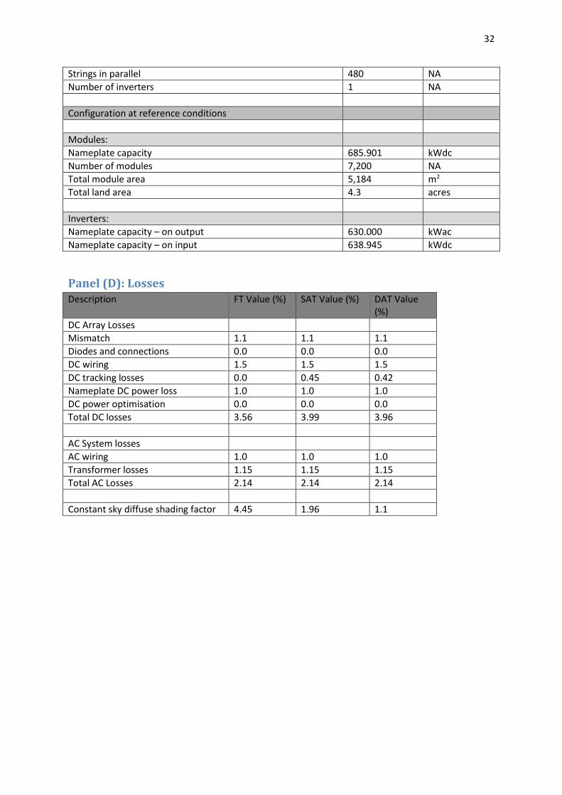
We utilised SAM’s 3d calculator to determine both near object direct beam and

constant sky diffuse shading losses for the three representative arrays. The constant sky

diffuse shading losses for the three representative arrays are reported in the last row of Panel

(D), Appendix A and are 4.45, 1.96 and 1.1 per cent, respectively, for the representative FT,

SAT and DAT arrays.

The near object direct beam shading losses determined for the three representative

arrays are documented in Table 3, Panels (A), (B) and (C) for the FT, SAT and DAT arrays.

It should be noted that in all three panels, the values of 100 per cent that are shaded in red

represent periods with complete shading. These arise in the early morning and early evening

hours, with some further constriction to operational hours also arising in winter relative to

summer. Values of zero indicate no shading impacts and partial near object shading effects

are represented by values between zero and 100, with larger impacts associated with higher

magnitude values.

In general, the DAT array (Panel C) has the lowest shading impacts in the early

morning and early evening hours when compared to the shading effects on both the FT and

SAT arrays. The SAT array has the next lowest shading impacts with the FT array

15

experiencing the highest near object shading effects. Note that this outcome was also

observed in the constant shy diffuse shading loss percentages reported above. Of particular

interest for PV yields projections is that the representative FT array experiences very little or

no near-object direct beam shading over the period 9 AM to 2 PM. In contrast, the

representative SAT and DAT arrays experience very little or no near-object direct beam

shading over slightly broader time horizons of 8 AM to 3 PM and 7 AM to 4 PM,

respectively.

Table3. Direct beam near-object shading factors for Gatton

arrays (Percentage)

Panel (A): Direct beam shading factors: representative FT array

Panel (B): Direct beam shading factors: representative SAT array

Panel (C): Direct beam shading factors: representative DAT sub-array

Month 5:00 AM 6:00 AM 7:00 AM 8:00 AM 9:00 AM 10:00 AM 11:00 AM 12:00 PM 1:00 PM 2:00 PM 3:00 PM 4:00 PM 5:00 PM 6:00 PM

JAN 100 0.0 0.0 0.0 0.0 0.0 0.0 0.0 0.0 0.0 0.0 0.0 0.0 100

FEB 100 0.0 0.0 0.0 0.0 0.0 0.0 0.0 0.0 0.0 0.0 0.0 0.0 100

MAR 100 0.0 0.0 0.0 0.0 0.0 0.0 0.0 0.0 0.0 0.0 0.0 0.0 100

APR 100 11.7 0.0 0.0 0.0 0.0 0.0 0.0 0.0 0.0 0.0 0.0 67.0 100

MAY 100 83.5 4.7 0.0 0.0 0.0 0.0 0.0 0.0 0.0 0.6 36.5 100 100

JUN 100 100 39.6 1.2 0.0 0.0 0.0 0.0 0.0 0.1 3.9 56.1 100 100

JUL 100 100 33.6 0.6 0.0 0.0 0.0 0.0 0.0 0.0 1.3 42.3 100 100

AUG 100 94.7 0.1 0.0 0.0 0.0 0.0 0.0 0.0 0.0 0.0 2.8 100 100

SEP 100 0.0 0.0 0.0 0.0 0.0 0.0 0.0 0.0 0.0 0.0 0.0 14.7 100

OCT 100 0.0 0.0 0.0 0.0 0.0 0.0 0.0 0.0 0.0 0.0 0.0 0.0 100

NOV 0.0 0.0 0.0 0.0 0.0 0.0 0.0 0.0 0.0 0.0 0.0 0.0 0.0 100

DEC 100 0.0 0.0 0.0 0.0 0.0 0.0 0.0 0.0 0.0 0.0 0.0 0.0 100

Month 5:00 AM 6:00 AM 7:00 AM 8:00 AM 9:00 AM 10:00 AM 11:00 AM 12:00 PM 1:00 PM 2:00 PM 3:00 PM 4:00 PM 5:00 PM 6:00 PM

JAN 3.5 0.0 0.0 0.0 0.0 0.0 0.0 0.0 0.0 0.0 0.0 0.0 0.0 5.2

FEB 100 0.0 0.0 0.0 0.0 0.0 0.0 0.0 0.0 0.0 0.0 0.0 0.0 3.6

MAR 100 0.0 0.0 0.0 0.0 0.0 0.0 0.0 0.0 0.0 0.0 0.0 0.0 100

APR 100 0.0 0.0 0.0 0.0 0.0 0.0 0.0 0.0 0.0 0.0 0.0 39.7 100

MAY 100 5.3 0.0 0.0 0.0 0.0 0.0 0.0 0.0 0.0 0.0 34.2 100 100

JUN 100 100 8.8 0.0 0.0 0.0 0.0 0.0 0.0 0.0 0.5 53.2 100 100

JUL 100 100 5.1 0.0 0.0 0.0 0.0 0.0 0.0 0.0 0.0 31.5 100 100

AUG 100 0.7 0.0 0.0 0.0 0.0 0.0 0.0 0.0 0.0 0.0 1.4 100 100

SEP 100 0.0 0.0 0.0 0.0 0.0 0.0 0.0 0.0 0.0 0.0 0.0 32.4 100

OCT 0.8 0.0 0.0 0.0 0.0 0.0 0.0 0.0 0.0 0.0 0.0 0.0 0.0 100

NOV 0.0 0.0 0.0 0.0 0.0 0.0 0.0 0.0 0.0 0.0 0.0 0.0 0.0 100

DEC 0.1 0.0 0.0 0.0 0.0 0.0 0.0 0.0 0.0 0.0 0.0 0.0 0.0 10.9

16

It should be noted that in the simulations performed for this paper, we did not include

any self-shading effects because such effects are not calculated for the DAT systems in the

most current version of SAM. However, SAM does calculate self-shading losses for both FT

and SAT arrays and other research indicates average self-shading losses of a tenth of one per

cent for the representative FT array and one per cent for the representative SAT array

(Gilman, 2015, Ch. 7.3).

The reason why self-shading losses are greater for the SAT array is that it can rotate

to track the azimuth angle of the sun, thereby producing greater yield in the early morning

and early evening hours when self-shading effects are most prevalent. Thus, the reduction in

output due to self-shading is subsequently greater in the case of SAT array when compared

with the FT array whose azimuth (and tilt) angle are fixed throughout the day and the system

cannot track the sun’s position.

In general, this outcome would be expected to be magnified further in the case of the

DAT array whose tilt and azimuth angles can track the sun’s zenith and azimuth angles over

the day, thus being more susceptible to potentially larger output reductions in early morning

and evening hours because of self-shading effects than in the case of the SAT array.

However, potentially moderating this effect is the fact that the DAT trackers are located

further apart than the rows of FT and SAT arrays. In modelling self-shading, the row spacing

between the rows of the FT arrays were determined to be 4.3 meters while the equivalent

spacing for the SAT array was determined to be 7.3 meters. In contrast, the shortest distance

between individual DAT trackers was determined to be around 10.5 meters on a diagonal

orientation and around 20.6 meters using a vertical orientation. More generally, the

investigation and quantifying of self-shading impacts (including ground reflected shading) on

the solar PV yield of the three technologies installed at GSRF is an ongoing research

programme.

Month 5:00 AM 6:00 AM 7:00 AM 8:00 AM 9:00 AM 10:00 AM 11:00 AM 12:00 PM 1:00 PM 2:00 PM 3:00 PM 4:00 PM 5:00 PM 6:00 PM

JAN 8.8 2.2 0.7 0.2 0.0 0.0 0.0 0.0 0.0 0.0 0.0 0.0 0.0 0.0

FEB 100 3.1 0.8 0.0 0.0 0.0 0.0 0.0 0.0 0.0 0.0 0.0 0.0 0.0

MAR 100 2.5 0.0 0.0 0.0 0.0 0.0 0.0 0.0 0.0 0.0 0.0 0.0 100

APR 100 5.6 0.0 0.0 0.0 0.0 0.0 0.0 0.0 0.0 0.0 0.0 0.0 100

MAY 100 15.1 0.0 0.0 0.0 0.0 0.0 0.0 0.0 0.0 0.0 0.0 100 100

JUN 100 100 0.0 0.0 0.0 0.0 0.0 0.0 0.0 0.0 0.0 0.0 100 100

JUL 100 100 0.0 0.0 0.0 0.0 0.0 0.0 0.0 0.0 0.0 0.0 100 100

AUG 100 13.6 0.0 0.0 0.0 0.0 0.0 0.0 0.0 0.0 0.0 0.0 100 100

SEP 100 0.0 0.0 0.0 0.0 0.0 0.0 0.0 0.0 0.0 0.0 0.0 0.0 100

OCT 5.0 1.7 0.0 0.0 0.0 0.0 0.0 0.0 0.0 0.0 0.0 0.0 0.0 100

NOV 7.5 1.5 0.5 0.0 0.0 0.0 0.0 0.0 0.0 0.0 0.0 0.0 0.0 100

DEC 7.8 1.8 0.6 0.0 0.0 0.0 0.0 0.0 0.0 0.0 0.0 0.0 0.0 0.0

17

DC and AC electrical losses

We have also adopted the following values for derating DC array output associated

with DC electrical losses of between 3.56 and 3.99 per cent, depending upon the array

technology and AC electrical losses of 2.14 per cent. Details of specific settings are listed in

Appendix A, Panel (D). It should be recalled that the DC ‘Mismatch’ and ‘Nameplate’ loss

factors were partially reduced to ensure that net losses were zero when the modification were

made to ensure that the augmented soiling loss factors adjusted for local spectrum were non-

negative. More information about typical loss factor settings for Solar PV simulations can be

found in Thevenard et al (2010), Tapia Hinojosa (2014) and ARUP (2015, Section 4.2).

(3.2) Assessment of Simulated Annual Production Levels of the

Different Representative Solar PV Arrays

Once all the required inputs have been made available to SAM, simulations can be

performed to assess the production outcomes of each representative solar PV technology.

The production results from the SAM modelling are reported in Table 4, Panels (A), (B) and

(C) for the low, medium and high soiling scenarios.

Given the focus in economic viability studies on revenue earnt from electricity

supplied directly to the grid, we calculate annual electricity production but exclude any

electricity used internally by the system at night which is represented as a negative output in

the annual production figures compiled by SAM. We calculate the annual production levels

by aggregating the hourly system output after zeroing out any negative hourly production

entries associated with internal consumption of electricity by the system at night. Thus, this

production concept reflects an energy sent-out production concept, that is, the electricity

exported to the grid during the day that is available to earn revenue by servicing demand.

Two particular revenue streams are envisaged. The first is revenue attributed to the

solar array associated with reduction in grid off-take of electricity which is subsequently

replaced by electricity produced by the solar array. The second revenue stream is revenue

from the sale of Large-Scale Generation Certificates (LGC) through the production of eligible

renewable energy under the Australian Government’s Large-Scale Renewable Energy Target

(LRET) scheme (CER, 2016).

The second last row of each panel of Table 4 contains the average production levels

whilst the last row in each panel contains aggregate total production results calculated for

18

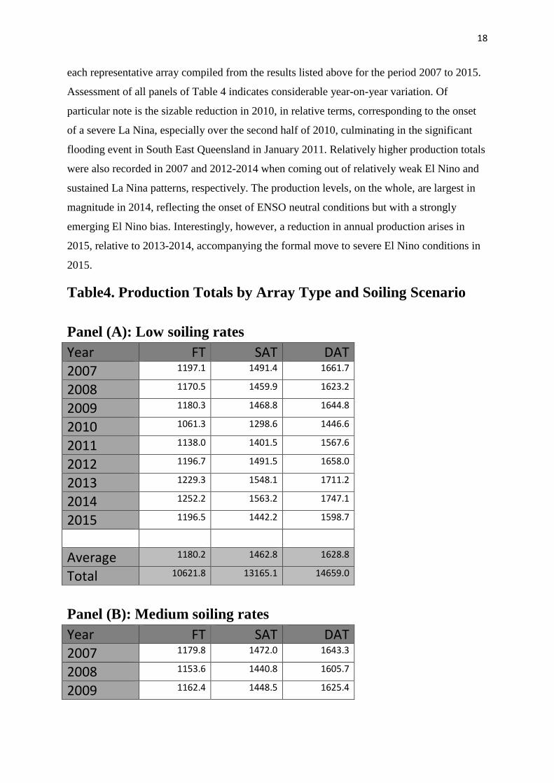
each representative array compiled from the results listed above for the period 2007 to 2015.

Assessment of all panels of Table 4 indicates considerable year-on-year variation. Of

particular note is the sizable reduction in 2010, in relative terms, corresponding to the onset

of a severe La Nina, especially over the second half of 2010, culminating in the significant

flooding event in South East Queensland in January 2011. Relatively higher production totals

were also recorded in 2007 and 2012-2014 when coming out of relatively weak El Nino and

sustained La Nina patterns, respectively. The production levels, on the whole, are largest in

magnitude in 2014, reflecting the onset of ENSO neutral conditions but with a strongly

emerging El Nino bias. Interestingly, however, a reduction in annual production arises in

2015, relative to 2013-2014, accompanying the formal move to severe El Nino conditions in

2015.

Table4. Production Totals by Array Type and Soiling Scenario

Panel (A): Low soiling rates

Year FT SAT DAT

2007 1197.1 1491.4 1661.7

2008 1170.5 1459.9 1623.2

2009 1180.3 1468.8 1644.8

2010 1061.3 1298.6 1446.6

2011 1138.0 1401.5 1567.6

2012 1196.7 1491.5 1658.0

2013 1229.3 1548.1 1711.2

2014 1252.2 1563.2 1747.1

2015 1196.5 1442.2 1598.7

Average 1180.2 1462.8 1628.8

Total 10621.8 13165.1 14659.0

Panel (B): Medium soiling rates

Year FT SAT DAT

2007 1179.8 1472.0 1643.3

2008 1153.6 1440.8 1605.7

2009 1162.4 1448.5 1625.4

19

2010 1046.2 1281.3 1430.3

2011 1121.5 1382.7 1549.6

2012 1179.8 1472.3 1637.7

2013 1211.7 1528.3 1693.2

2014 1234.2 1543.0 1727.9

2015 1179.7 1424.6 1582.5

Average 1163.2 1443.7 1610.6

Total 10468.9 12993.6 14495.6

Panel (C): High soiling rates

Year FT SAT DAT

2007 1151.3 1438.9 1610.8

2008 1125.3 1408.3 1574.1

2009 1133.1 1414.8 1591.9

2010 1021.1 1252.3 1401.6

2011 1094.3 1351.2 1518.0

2012 1151.4 1439.6 1603.1

2013 1182.2 1494.2 1660.6

2014 1204.3 1508.6 1693.5

2015 1151.8 1394.2 1553.4

Average 1135.0 1411.4 1578.6

Total 10214.7 12702.2 14207.1

The system-wide impacts of soiling can also be discerned from Table 4. Under the

low soiling scenario, average annual production levels of 1180.2, 1462.8 and 1628.8 MWh

were reported in Panel (A) for the representative FT, SAT and DAT arrays, respectively.

Similarly, total production values for the period 2007 to 2015 of 10621.8, 13165.1 and

14659.0 MWh were also recorded. Comparison of these production results with the

equivalent values associated with the medium and high soiling scenarios point to reductions

in both average annual and total production for all three representative arrays. Furthermore,

the rate of reduction in average annual and total production relative to the low soiling

scenario increases with the level of soiling.

20

Specifically, for the representative FT array, average annual production was reduced

by 1.4 and 3.8 per cent, relative to the low soiling scenario’s average annual production level

cited above. For the representative SAT array, the equivalent reduction in annual average

production was 1.3 and 3.5 per cent, respectively. In the case of the representative DAT

array, the reduction was 1.1 and 3.1 per cent. Using total production instead of average

annual production produces similar percentage sized reductions. Moreover, if we compare the

percentage reduction in both production measures for the high soiling scenario relative to the

medium soiling scenario, the percentage reductions are in the order of 2.4, 2.2 and 2.0 per

cent, respectively, for the representative FT, SAT and DAT arrays.

These results indicate that the output of the representative FT array is more adversely

affected by increased soiling relative to the solar PV yields of the representative SAT and

DAT arrays. This is seen in the higher percentage reduction rates associated with the FT array

when compared with the other two representative arrays. Furthermore, the SAT array is more

adversely affected by soiling than is the DAT array with the former recording higher

percentage reductions in solar PV yield than the latter. Thus, some tracking ability can help

partially insulate against the adverse impacts of module soiling on solar PV yield.

Recall that the key metric often sought when comparing the performance of solar PV

tracking systems relative to a benchmark FT system is the extent to which output of the

tracking systems exceeds that of the benchmark FT system. These results are reported in

Panels (A)-(C) of Table 5 in relation to the annual production data reported in Table 4 for the

low, medium and high soiling scenarios, respectively. The data in Table 5 documents the

percentage increase in output of the SAT and DAT trackers relative to the output of the FT

array. As such, in Table 5, Panel (A) for year 2007, the values of 24.6% and 38.8% indicate

that the output of the SAT and DAT arrays recorded in Table 4, Panel (A) for year 2007 (e.g.

1491.4 and 1661.7 MWh’s) are 24.6 and 38.8 per cent higher than the corresponding output

of the FT array (e.g. 1197.1 MWh). Note that for the SAT technology, the percentages

reported in the second column of Table 5 are calculated for each year as:

.100

Pr

PrPr

FT

FTSAT

SATod

ododPercentage (3)

where 'Pr' FTod and 'Pr' SATod refer to the yearly annual production data reported in Table 4

for the FT and SAT arrays. The percentages for the DAT technology listed in Column 3 of

21

Table 5 can also be calculated in a similar manner after replacing the ‘SAT’ subscripts in (3)

with ‘DAT’ subscripts.

Examination of Table 5 once again indicates some year-on-year variation in the

percentage figures and also by soiling scenario. For the SAT array, they are bounded between

20.5 and 25.9 per cent for the low soiling scenario [Panel (A)], between 20.8 and 26.1 per

cent for medium soiling scenario [Panel (B)], and between 21.0 and 26.4 per cent for the high

soiling scenario [Panel (C)]. The average percentage increase in solar PV yield for this array

type relative to the solar PV yield of the benchmark representative FT array for the period

2007-2015 are listed in the last row of each panel in Table 5 and are 23.9, 24.1 and 24.3 per

cent, respectively, for the low, medium and high soiling scenarios. Thus, the average results

listed in Table 5 for the representative SAT array generally increases with the soiling scenario

indicating that the SAT array tracking behaviour improves the solar PV yield relative to the

benchmark FT array as the level of soiling increases, at least, for the monthly soiling ranges

outlined in Table 2.

In the case of the representative DAT array, the results in Table 5 are bounded

between 33.6 and 39.5 per cent for the low soiling scenario [Panel (A)], between 34.1 and

40.0 per cent for medium soiling scenario [Panel (B)], and between 34.9 and 40.6 per cent for

the high soiling scenario [Panel (C)]. The average percentage increase in solar PV yield for

this array relative to production from the benchmark FT array for the period 2007-2015 are

38.0, 38.4 and 39.1 per cent, respectively, for the low, medium and high soiling scenarios.

Once again, the increase in the average value with soiling scenario indicates that the DAT

array’s tracking behaviour improves the solar PV yield relative to the FT array as the level of

soiling increases. Furthermore, relative to the output of the benchmark FT array, the higher

percentage values for the DAT array in Table 5 also clearly underpin the greater production

of electricity coming from the DAT array compared with the SAT array.

Table5. Percentage Change in Production for SAT and DAT

Tracking Systems Relative to FT System by Soiling Scenario

Panel (A): Low soiling rates

Year SAT DAT

2007 24.6 38.8

2008 24.7 38.7

22

2009 24.4 39.4

2010 22.4 36.3

2011 23.1 37.7

2012 24.6 38.6

2013 25.9 39.2

2014 24.8 39.5

2015 20.5 33.6

Average 23.9 38.0

Panel (B): Medium soiling rates

Year SAT DAT

2007 24.8 39.3

2008 24.9 39.2

2009 24.6 39.8

2010 22.5 36.7

2011 23.3 38.2

2012 24.8 38.8

2013 26.1 39.7

2014 25.0 40.0

2015 20.8 34.1

Average 24.1 38.4

Panel (C): High soiling rates

Year SAT DAT

2007 25.0 39.9

2008 25.2 39.9

2009 24.9 40.5

2010 22.6 37.3

2011 23.5 38.7

2012 25.0 39.2

2013 26.4 40.5

2014 25.3 40.6

2015 21.0 34.9

Average 24.3 39.1

23

The average results cited in the last row of each panel of Table 5 are broadly

consistent with findings in the literature. Manufacturer’s claims often assert increases of up to

30% for single axis tracking systems and up to 40% for dual axis tracking systems (Sabry and

Raichle, 2013). Robinson and Raichle (2012) cite values from studies for SAT systems of

between 29.3% and 42% and between 29.2% and 54%, depending upon the geographic

location and climatic conditions underpinning the studies. Mousazadeh et al. (2009, p. 1802)

cite general evidence pointing to gains of between 30% and 40% in good areas (and

conditions) and in the low 20% range in poor conditions such as cloudy and hazy locations.

More generally, in their detailed survey of efficiency gains reported in the literature relating

to active solar tracking systems, they report evidence pointing to gains in production in the

range of 20% to 30% for single axis tracking systems and between 30% and 45% for two axis

tracking systems (Mousazadeh et al., 2009, pp. 1807-1810). Using these results as a broad

guide, the average results reported in Table 5 would seem to be within the mid-range of these

estimates cited in the broader literature.

(3.3) Assessment of Simulated Annual Capacity Factor Outcomes

Once the annual production outcomes have been calculated for the three

representative arrays at GSRF, it is a simple process to calculate the annual capacity factor

(ACF) outcomes of each representative system. The ACF is calculated by the following

equation:

,

_8760

Pr_

CapacitySystem

odAnnualACF (4)

where ‘8760’ represents the number of hours in a year assuming a 365 day year. Note, in this

context, that for the leap years 2008 and 2012, the additional day corresponding to the 29th of

February was dropped from the analysis. Note also in the denominator of (4), the kW system

capacity concept we use in calculating the ACF is the sent-out capacity linked to the kWac

maximum capacity of each of the inverters. This can be contrast with the use of the Array

kWdc maximum capacity which is used to calculate the ACF results reported in the summary

table generated by the SAM software. The ACF results for the three representative arrays are

reported in Table 6, Panels (A) –(C) for the low, medium and high soiling scenarios. Note

that the production concept [e.g. variable 'Pr_' odAnnual in (4)] is based on the annual

24

production totals for each soiling scenario cited in Table 4 and variable '_' CapacitySystem

corresponds to the 630 kWac capacity limit of the inverter.

Table6. Energy Sent-out ACF by Representative Array Type by

Soiling Scenario1

Panel (A): ACF: Low soiling rates

Year FT SAT DAT

2007 21.7 27.0 30.1

2008 21.7 27.0 30.1

2009 22.3 27.8 31.1

2010 19.2 23.5 26.2

2011 20.6 25.4 28.4

2012 21.7 27.0 30.0

2013 22.3 28.1 31.0

2014 22.7 28.3 31.7

2015 21.7 26.1 29.0

Average 21.5 26.7 29.7

Panel (B): ACF: Medium soiling rates

Year FT SAT DAT

2007 21.4 26.7 29.8

2008 21.4 26.7 29.7

2009 22.0 27.4 30.7

2010 19.0 23.2 25.9

2011 20.3 25.1 28.1

2012 21.4 26.7 29.7

2013 22.0 27.7 30.7

2014 22.4 28.0 31.3

2015 21.4 25.8 28.7

1 Because of satellite problems, data was missing from the BOM’s hourly solar irradiance dataset for: (1) year 2008, 14 to 17 of March and 10-13 of April, representing 192 hours of missing data; and (2) year 2009, 17-18 of February, 12 and 16-27 of November, representing 360 hours of missing data. The ACF calculations in Table 6 for years 2008 and 2009 were adjusted appropriately to account for these missing observations, with the number of hours in the denominator of equation (4) being reduced from 8760 to 8568 (e.g. 8760-192) and 8400 (e.g. 8760-360) for years 2008 and 2009, respectively.

25

Average 21.2 26.4 29.4

Panel (C): ACF: High soiling rates

Year FT SAT DAT

2007 20.9 26.1 29.2

2008 20.8 26.1 29.2

2009 21.4 26.7 30.1

2010 18.5 22.7 25.4

2011 19.8 24.5 27.5

2012 20.9 26.1 29.0

2013 21.4 27.1 30.1

2014 21.8 27.3 30.7

2015 20.9 25.3 28.1

Average 20.7 25.8 28.8

Inspection of Table 6 points to considerable variation in the ACF’s on a year-by-year

basis, as was also observed with the production totals listed in Table 4. Specifically, and

mirroring the production outcomes, the lowest ACF’s were recorded in year 2010 and the

highest were recorded in 2014. For the low, medium and high soiling scenarios, the ACF

results for the benchmark FT technology fall within the range 19.2% to 22.7%, 19.0% to

22.4% and 18.5% to 21.8%. For the period 2007 to 2015, the average ACF values for the

representative FT array were determined to be 21.5, 21.2 and 20.7 per cent for the low,

medium and high soiling scenarios.

In the case of the representative SAT array, the equivalent ACF outcomes for each

soiling scenario were in the range of 23.5% to 28.3%, 23.2% to 28.0% and 22.7% to 27.3%,

respectively, and with average ACF outcomes being 26.7, 26.4 and 25.8 per cent. For the

representative DAT array, the equivalent ACF outcomes were in the range of 26.2% to

31.7%, 25.9% to 31.3% and 25.4% to 30.7%, respectively. The average ACF outcomes by

soiling scenario for the representative DAT array were 29.7, 29.4 and 28.8 per cent.

It is apparent from these results that for all three representative arrays, the average

ACF results and their range clearly diminish as the level of module soiling increases.

Moreover, mirroring the production results examined in the previous section, the ACF

outcomes are highest for the representative DAT array, being in the range of 28.8 to 29.7 per

26

cent, in average terms, depending on module soiling. This is followed by the results for the

representative SAT array which, in average terms, are in the range 25.8 to 26.7 per cent, once

again depending on soiling effects. Finally, the representative FT array clearly has the lowest

results with average ACF results for the period 2007-2015 in the range of 20.7 to 21.5 per

cent, depending on the extent of module soiling.

(4) Conclusions

Economic assessment of the viability of different types of solar PV tracking

technologies centres on an assessment of whether the annual production of the different

tracking technologies is increased enough relative to the benchmark FT system to compensate

for the higher cost of installation and operational expenditures incurred by the tracking

systems. To assess this, in the first instance, simulation modelling of the PV yield of the

different solar PV systems needs to be performed. In this paper we restricted attention to an

assessment of the production results of three representative 630 kW FT, SAT and DAT arrays

located at UQ Gatton campus.

NREL’s SAM model was used to simulate electricity production from the three

representative solar PV systems installed at Gatton. Data relating to hourly solar irradiance

data, weather data, and surface albedo data for Gatton was sourced from the BOM and

NASA. Technical data relating to both module and inverter characteristics were sourced from

both the module and inverter manufacturer’s data sheets. Impacts of soiling and near-object

shading were also accounted for in assessing solar PV yield.

Three broad module soiling scenarios were incorporated into the modelling. These

were a low, medium and high module soiling scenario. These soiling scenarios were linked

to a hypothesised cleansing effect of rainfall and were also augmented to account for energy

gains and losses associated with divergence of local spectrum conditions from STC spectrum

conditions. These low, medium and high augmented soiling losses produced average

annualised soiling rates of 1.7, 3.2 and 5.7 per cent, respectively, albeit with much more

variability arising on a month-by-month basis.

A key finding from the SAM simulations was that over the period 2007 to 2015,

average increases in annual production of between 23.9 and 24.3 per cent and 38.0 and 39.1

per cent were obtained for the SAT and DAT tracking systems relative to the FT system,

27

depending on module soiling rates. These results fell within the mid-range of estimates for

these types of solar PV technologies identified in the broader literature.

ACF results were also calculated for the three representative arrays being considered.

The representative FT array had the lowest recorded ACF values, in the range 20.7 to 21.5

per cent, depending on the rate of module soiling. The representative SAT array had the next

lowest average ACF values, in the range 25.8 to 26.7 per cent, once again, depending upon

module soiling rates. The highest ACF outcomes were recorded by the representative DAT

array with average ACF results in the range of 28.8 to 29.7 per cent.

A key finding was that the output of the representative FT array is more adversely

affected by increased soiling relative to the solar PV yields of the representative SAT and

DAT arrays. Moreover, the SAT array was more adversely affected by soiling than was the

DAT array. This suggested that some tracking ability could help partially insulate solar PV

yields against the adverse impacts of module soiling. Future research will compare these

predictions to actual data from the GSRF array.

28

References

ACT: Australian Capital Territory (2016) ‘: ACT Government, Environment and Planning

Directorate, Environment, Large Scale Solar.’ Available at:

http://www.environment.act.gov.au/energy/cleaner-energy/large-scale-solar.

AGL (2015) ‘Fact Sheet: Nyngan Solar Plant.’ Available at:

https://www.agl.com.au/~/media/AGL/About%20AGL/Documents/How%20We%20Source

%20Energy/Solar%20Community/Nyngan%20Solar%20Plant/Factsheets/2014/Nyngan%20F

act%20Sheet%20v7.pdf.

ARENA (2016) ‘Australian Government Australian Renewable Energy Agency.’ Available

at: http://arena.gov.au/..

ARUP (2015) ‘Energy Yield Simulations, Module Performance Comparison for Four Solar

PV Module Technologies.’ Arup (Pty) Ltd Consulting Engineers, Johannesburg, South

Africa, May 2015. Available at:

http://www.bizcommunity.com/f/1505/Module_Performance_Comparison_for_Four_Solar_P

V_Module_Technologies_08-0....pdf.

Australian Government Clean Energy Regulator: CER (2016) ‘Large-scale Renewable

Energy Target.’ Available at: http://www.cleanenergyregulator.gov.au/RET/About-the-

Renewable-Energy-Target/How-the-scheme-works/Large-scale-Renewable-Energy-Target.

Accessed 25-5-2016.

Bureau of Meteorology: BOM (2015) ‘Australian Hourly Solar Irradiance Gridded Data.’

Available at: http://www.bom.gov.au/climate/how/newproducts/IDCJAD0111.shtml.

CEFC (2016) ‘Clean Energy Finance Corporation.’ Available at:

http://www.cleanenergyfinancecorp.com.au/.

Dobos, A (2012) ‘An improved Coefficient Calculator for the California Energy Commission

6 Parameter Photovoltaic Module Model’. Journal of Solar Energy Engineering, 132(2).

First Solar (2015) ‘Module Characterisation: Energy Prediction Adjustment for Local

Spectrum’. First Solar Document Number PD 5-423.

Gilman, P. (2015) ‘SAM Photovoltaic Model Technical Reference.’ National Renewable

Energy laboratory (NREL), May. Available at: http://www.nrel.gov/docs/fy15osti/64102.pdf.

Green Energy Markets (2015) ‘Renewables target needs 3,800MW of large scale renewables

within 12 months.’ Available at: http://greenmarkets.com.au/news-events/renewables-target-

needs-3800mw-of-large-scale-renewables-within-12-months.

Kimber, A., Mitchell, L., Nogradi, S., and H. Wenger (2006),’ The effect of soiling on large

grid-connected photovoltaic systems in California and the southwest region of the United

States.’ In Conference Record of the 2006 IEEE 4th World Conference on Photovoltaic

29

Energy Conversion, Waikoloa, HI, 2006. Available at:

http://ieeexplore.ieee.org/stamp/stamp.jsp?tp=&arnumber=4060159.

Mousazadeh, H., Keyhani, A., Javadi, A., and H. Mobli (2009) ‘A review of principle and

sun-tracking methods for maximising solar systems output’, Renewable and Sustainable

Energy Reviews, 13, pp. 1800-1818.

NASA (2015) ‘Albedo 16-Day L3 Global 0.05Deg CMG’. Available at:

https://lpdaac.usgs.gov/dataset_discovery/modis/modis_products_table/mcd43c3.

RMI: Rocky Mountain Institute and Georgia Tech Research Institute (2014) ‘Lessons From

Australia: Reducing Solar PV Costs Through Installation Labour Efficiency.’ Available at:

http://www.rmi.org/Knowledge-Center/Library/2014-11_RMI-AustraliaSIMPLEBoSFinal.

Reda, I., and A. Andreas (2003) ‘Solar position algorithm for solar radiation applications’,

National Renewable Energy Laboratory (NREL), Technical Report NREL/TP-560-34302.

Available at: http://www.nrel.gov/docs/fy08osti/34302.pdf.

Robinson, J.W., and B.W. Raichle (2012) ‘Performance Comparison of Fixed, 1-, and 2-Axis

Tracking Systems for Small Photovoltaic Systems with Measured Direct Beam Fraction.’

Proceedings of 42nd ASES Annual Conference, Denver, Colorado, May 2012. Available at:

http://ases.conference-

services.net/resources/252/2859/pdf/SOLAR2012_0261_full%20paper.pdf.

Sabry, M. S., and B. W. Raichle (2013) ‘Determining the Accuracy of Solar Trackers’.

Proceedings of 42nd ASES Annual Conference, Baltimore, Maryland, April 2013. Available

at: http://proceedings.ases.org/wp-content/uploads/2014/02/SOLAR2013_0075_final-

paper.pdf.

Sallaberry, F., de Jalon, A.G., Torres, J-L., and R. Pujol-Nadal (2015) ‘Optical losses due to

tracking error estimation for a low concentrating solar collector.’ Energy Conservation and

Management, 92, pp. 194-206.

Stafford, B., Davis, M., Chambers, J., Martinez, M., and D. Sanchez (2009) ‘Tracker

accuracy: field experience, analysis, and correlation with meteorological conditions.’

Photovoltaic Specials Conference (PVSC), 34 IEEE, June 2009. Available at:

http://ieeexplore.ieee.org/stamp/stamp.jsp?tp=&arnumber=5411362.

Tapia Hinojosa., M (2014) ‘Evaluation of Performance Models against Actual Performance

of Grid Connected PV Systems.’Master’s Thesis, Institute of Physics, Carl von Ossietzky

Universität Oldenburg. Available at: http://oops.uni-

oldenburg.de/2433/7/Thesis_TapiaM.pdf.

Thevenard, D., Driesse, A., Turcotte, D., and Y. Poissant (2010) ‘Uncertainty in Long-term

Photovoltaic Yield Projections.’ CanmetENERGY, Natural Resources Canada, March.

Available at:

https://www.nrcan.gc.ca/sites/www.nrcan.gc.ca/files/canmetenergy/files/pubs/2010-122.pdf.

30

UQ (2015a) ‘UQ, First Solar to build world-leading research centre.’ Available at:

https://www.uq.edu.au/news/article/2013/10/uq-first-solar-build-world-leading-research-

centre

UQ (2015b) ‘Fixed Tilt Array.’ Available at: https://www.uq.edu.au/solarenergy/pv-

array/content/fixed-tilt-array.

UQ (2015c) ‘Single Axis tracking Array.’ Available at:

https://www.uq.edu.au/solarenergy/pv-array/content/single-axis-tracking-array.

UQ (2015d) ‘Dual Axis tracking Array.’ Available at: https://www.uq.edu.au/solarenergy/pv-

array/content/dual-axis-array.

31

Appendix A. SAM Design and Parameter Settings

Panel (A): Modules Description Value Measurement

Unit

Module description - Thin Film Cadmium Telluride module First Solar FS-395 PLUS (95 W)

NA

Cell type – CdTe NA NA

Module area 0.72 m2

Nominal operating cell temperature 45 oC

Maximum power point voltage (Vmp) 45.8 V

Maximum power point current (Imp) 2.08 A

Open circuit voltage (Voc) 58 V

Short circuit current (Isc) 2.29 A

Temperature coefficient of Voc -0.28 %/ oC

Temperature coefficient of Isc 0.04 %/ oC

Temperature coefficient of maximum power point -0.29 %/ oC

Number of cells in series 146 NA

Standoff height Ground or rack mounted

NA

Approximate installation height one story building height or lower

NA

Panel (B): Inverters Description Value Measurement

Unit

Inverter type SMA Sunny Central 720CP XT

NA

Maximum AC power output 630,000 Wac

Manufacturer efficiency 98.6 %

Maximum DC input power 638,945 Wdc

Nominal AC voltage 324 Vac

Maximum DC voltage 1000 Vdc

Maximum DC current 1400 Adc

Minimum MPPT DC voltage 577 Vdc

Nominal DC voltage 577 Vdc

Maximum MPPT DC voltage 850 Vdc

Power consumption during operation 1950 Wdc

Power consumption at night 100 Wac

Panel (C): System Design Description Value Measurement

Unit

Modules per string 15 NA

32

Strings in parallel 480 NA

Number of inverters 1 NA

Configuration at reference conditions

Modules:

Nameplate capacity 685.901 kWdc

Number of modules 7,200 NA

Total module area 5,184 m2

Total land area 4.3 acres

Inverters:

Nameplate capacity – on output 630.000 kWac

Nameplate capacity – on input 638.945 kWdc

Panel (D): Losses Description FT Value (%) SAT Value (%) DAT Value

(%)

DC Array Losses

Mismatch 1.1 1.1 1.1

Diodes and connections 0.0 0.0 0.0

DC wiring 1.5 1.5 1.5

DC tracking losses 0.0 0.45 0.42

Nameplate DC power loss 1.0 1.0 1.0

DC power optimisation 0.0 0.0 0.0

Total DC losses 3.56 3.99 3.96

AC System losses

AC wiring 1.0 1.0 1.0

Transformer losses 1.15 1.15 1.15

Total AC Losses 2.14 2.14 2.14

Constant sky diffuse shading factor 4.45 1.96 1.1