1

Green Roof & Solar Array – Comparative Research Project

Final Report July 2021

2020/037855 / EPI R3 201920005

2

Prepared by:

Peter Irga – Chief Investigator

Robert Fleck – Principal Investigator

Eamonn Wooster – Ecologist

Fraser Torpy – Senior Lecturer

Hisham Alameddine – R&D Manager

Lucy Sharman – Sustainability Manager

With contributions by:

Natalie Killingsworth – Grad. Engineer

Stephanie Saadah – Grad. Engineer

Thomas Pettit – Research Scientist

Raissa Gill – Research Scientist

Mika Westerhausen - PhD Research Scientist

Jack Rojahn – Research Scientist

James Ball – Associate Professor

Ekaterina Arsentova – Grad. Engineer

Tuong (Cat) Chu – Grad. Engineer

Jock Gammon – Junglefy Co-Founder and Managing Director

Peter Flynn – Senior Project Manager

Graham Carter – Senior Technical Lead

Peter Zacharia – Sustainability Consultant

Angela Begg – Sustainability Consultant

Acknowledgements

The authors acknowledge the traditional custodians, the Gadigal people of the Eora Nation,

on whose land this work was conducted. The authors thank Giovanni Cercone, Luke Brown,

Martino Masini, Emmanuel Stathakis and Ana Curkovic for facilitating site access. Further

thanks to Harry Ritz and Poppy Danis from Junglefy for their support with facilitating the

research, as well as Nathan Sharman and Gabrielle Duani from UTS.

3

EXECUTIVE SUMMARY

Background

Green roofs and the integration of greenery into building structures is a vital component in

building resilient cities in a changing climate. However, there is currently a lack of research

that confirms many of the well understood (but often anecdotal) benefits of green roofs,

including hosting biodiversity, counteracting air pollution; reducing ambient temperatures

that contribute to the urban heat island effect, the provision of efficient renewable energies

and decreasing city-scape surface runoff from rainwater. With the support of the City of

Sydney, the work presented here describes studies conducted in collaboration with Lendlease,

Junglefy and the University of Technology Sydney to evaluate several performance

characteristics essential for determining the functionality of green roofs in Sydney Australia.

These research questions were explored by conducting comparative research on two identical

buildings of similar age, both located adjacent to one another in Barangaroo, - one with

photovoltaic panels (International House) and one integrating photovoltaic panels with a

green roof (Daramu House).

Urban biodiversity

One issue of pressing importance is the provision and preservation of biodiversity in urban

centres. In this study we observed that the presence of the green roof resulted in a nine-fold

increase in insect species diversity, as well as a four-fold increase in avian species diversity.

More surprisingly, the discovery of strong evidence of predatory activity indicates that an

entire food web may have been developing on the green roof. Additionally, the plant species

present underwent changes in succession throughout the duration of the experiment,

particularly in the shaded regions of the roof (i.e. beneath the solar panels) which are the most

difficult to cultivate and maintain. We observed Aptenia cordigolia (baby sun rose) increase

from a planting abundance of ~6%, to ~85% in these areas, indicating that the plant

community was self-regulating and adapting. This provides strong evidence of plant survival

into the future.

4

Air pollution

Green roofs are known for their potential to reduce air pollutant concentrations. In this study

nitrogen dioxide (NO2), ozone (O3) and particulate matter (PM2.5) were monitored on the two

buildings. Whilst NO2 was observed to be higher on the green roof than on the conventional

roof for as yet unknown reasons, O3 was significantly lower on the green roof, likely due to

plant uptake during photosynthesis. Whilst nearby construction works prevented us from

determining the effect of PM2.5 deposition on the plants, the recorded values were

incorporated into a pollution removal model, which predicted that the presence of plant

foliage on the green roof could mitigate up to 2.3, 6.9 and 0.5 Kg per year of NO2, O3 and

PM2.5, respectively.

Insulation

Our observations indicate the potential for urban heat island mitigation through the

application of urban green roofing. The measurements indicated that the two roofs

experienced similar solar thermal exposure. Surface temperatures of concrete flooring, and on

the exposed plant foliage indicated a significant reduction in temperature, in some instances

up to 20°C. A stratified thermal gradient was monitored to determine the vertical temperature

profile of the two roofs were determined. For temperatures below the solar panels, both the

average and maximum daily temperatures were significantly lower on the green roof than the

conventional roof. Minimum daily temperatures on the green roof, however, were higher than

those on the conventional roof. This highlights the insulative capacity of the green roof to not

only prevent heat transfer indoors, but to retain heat during colder periods.

Stormwater

Multiple models were employed to determine the effect of a green roof on roof stormwater

behaviour. Stormwater flowrate models (DRAINS and SWMM) indicated that the green roof

caused a significant reduction in the rate of water flow during storm events of various

magnitudes. Our findings indicated that the green roof could reduce flow rates in storm

events of up to a 1 in 40-year intensity by up to 600 L/s. It is thus likely that a considerable

reduction in storm flow burden on city underground stormwater management systems would

result from a mass adoption of green roofs in the Sydney CBD.

5

Stormwater pollution

Field observations of problematic metal pollutants demonstrated a significant reduction in

both soluble and insoluble copper entering the stormwater systems from the green roof when

compared to the conventional roof, as well as a significant reduction in insoluble zinc and

chromium, possibly due to sequestration or uptake by plant matter, however this was not

directly assessed in this project.

Renewable energy

The provision of renewable energy from both rooftops was substantial during the 8-month

monitoring period (69 and 59.5 MWh for the green and conventional roofs, respectively).

After correction for a range of factors that differed between the two roofs, the green roof

produced 9.5 MWh of electricity over the 8-month period more than the conventional roof,

corresponding to a retail market value of $2,595. Due to the surrounding urban geometries,

system performance was assessed under simulated lighting conditions, where the green roof

was, on average, 3.63 % more efficient on any given day over the 8-month monitoring

period. The environmental impact of this is substantial. The green and conventional roofs

mitigated the production of greenhouse gasses from conventional sources by 55.9 and 48.2

tonnes of e-CO2, respectively. The difference in energy generated is equivalent to 110 trees

planted, with an additional 1.1 t-CO2 potentially mitigated by photosynthetic activity of the

plant foliage on the green roof.

Conclusions

The benefits provided by green roofs are clearly substantial. Whilst we detected increased

biodiversity, reductions in some air pollutants, improved stormwater management, improved

building insulation and a surprisingly high increase in the rate of energy produced by the

solar array on the green roof, only a pair of single buildings was assessed. With the

widespread adoption of green roofs in cities, we predict that a synergistic effect amongst

buildings could be possible, whereby the ecosystem services provided would be multiplied.

With the rapidly unfolding climate crisis, it is abundantly clear that we need to do more to

reduce the contribution our cities make to these problems. For the size of the positive impacts

generated relative to the costs, green infrastructure is perhaps the easiest and most efficient

initiative we can make to help make our cities sustainable.

6

Contents 1 Introduction ..................................................................................................................................... 8

1.1 Site description .............................................................................................................................. 9

2 Biodiversity ................................................................................................................................... 12

2.1 Introduction ................................................................................................................................. 12

2.2 Methods....................................................................................................................................... 13

2.2.1 Biodiversity monitoring ........................................................................................................... 13

2.2.2 Data analysis ............................................................................................................................ 14

2.3 Results ......................................................................................................................................... 15

2.4 Findings....................................................................................................................................... 18

3 Air quality ..................................................................................................................................... 19

3.1 Introduction ................................................................................................................................. 19

3.1.1 Air pollution and green roofs ................................................................................................... 19

3.1.2 Quantifying air pollution removal by green roofs.................................................................... 20

3.1.3 Ozone removal by HVAC ........................................................................................................ 21

3.2 Methods....................................................................................................................................... 22

3.2.1 Ambient Air Quality monitoring .............................................................................................. 22

3.2.2 Big-leaf resistance model ......................................................................................................... 24

3.3 Results ......................................................................................................................................... 25

3.3.1 Air pollution removal by the green roof .................................................................................. 29

3.4 Findings....................................................................................................................................... 32

4 Thermal insulation ........................................................................................................................ 33

4.1 Introduction ................................................................................................................................. 33

4.2 Methods....................................................................................................................................... 34

4.2.1 Description and Temperature Sensors ..................................................................................... 34

4.2.2 Thermal imagery camera ......................................................................................................... 36

4.2.3 Thermal performance calculations ........................................................................................... 37

4.3 Results and Findings ................................................................................................................... 39

4.3.1 Thermal Performance - Theoretical ......................................................................................... 39

4.3.2 Thermal Performance – Observed ........................................................................................... 40

5 Stormwater Runoff ........................................................................................................................ 46

5.1 Introduction ................................................................................................................................. 46

5.2 Materials and Methods ................................................................................................................ 48

5.2.1 Flood study using DRAINS ..................................................................................................... 48

7

5.2.2 Model for Urban Stormwater Improvement Conceptualisation (MUSIC) .............................. 51

5.2.3 Elemental analysis ................................................................................................................... 53

5.2.4 StormWater Management Model (SWMM) ............................................................................ 56

5.3 Results & Findings ...................................................................................................................... 59

5.3.1 DRAINS modelling ................................................................................................................. 59

5.3.2 DRAINS modelling limitations: .............................................................................................. 62

5.3.3 MUSIC model and trace metal analysis ................................................................................... 62

5.3.4 SWMM Analysis ..................................................................................................................... 67

6 PV performance assessment .......................................................................................................... 71

6.1 Introduction ................................................................................................................................. 71

6.2 Materials and Methods ................................................................................................................ 72

6.3 Results ......................................................................................................................................... 75

6.4 System Considerations for Comparisons .................................................................................... 78

6.5 Findings....................................................................................................................................... 78

7 Conclusions and future directions ................................................................................................. 80

8. References ......................................................................................................................................... 82

8

1 Introduction

With the impending threat of climate change, one concept being explored to embed climate

resilience into the built environment is through the use of “green infrastructure” (GI). GI

involves incorporating aspects of nature into the built environment and aims to provide

environmental benefits (‘ecosystem services’) including hosting biodiversity; counteracting

air pollution; minimising ambient temperatures that contribute to the urban heat island effect;

the provision of efficient renewable energies; and decreasing city-scape surface runoff from

rainwater. Green roofs are a form of sustainable, low impact GI development, and their

integration into building structures may become a vital component in building resilient cities

in a changing climate.

Many green roof studies to date divide a single rooftop into green roof and non-green roof

sections to measure the differing effects, however, these studies are constrained by ‘spatial

confounding’ resulting from the proximity of the treatments leading to their effects

influencing one another. Conversely, studies that compare distinct buildings produce

comparisons with limited validity due to the buildings being too far apart or too different in

construction to be comparable. The current case study provided a unique opportunity to

measure two separate, but adjacent buildings exposed to the same environmental conditions,

in order to provide valid experimental data to contribute to the City of Sydney’s Green Roofs

and Wall Policy Implementation Plan.

This project thus represents a comparative study of Barangaroo Daramu House (Green roof)

and International House (Conventional roof). Both buildings support photovoltaic (PV)

panels, with Daramu House hosting, in addition, an extensive green roof. Data was collated to

compare the two roofs for:

9

1) Biodiversity

2) Air quality

3) Thermal insulation properties

4) Stormwater runoff

5) PV performance

This project is innovative due to the inclusion of a control building with equivalent structure

and age to allow the isolation of benefits provided by the green roof. Further, no previous

research within New South Wales, Australia has explored the knowledge gaps related to

integrated green roof effects on PV systems. The outcomes of this project will allow a better

understanding of integrating green roof solutions on buildings within the City of Sydney and

similar Australian metropolitan areas. There is evidence to suggest that integrating PV panels

and green roofs are beneficial to the city, however this has not been previously tested in

Australia, resulting in a lack of methodology for implementing urban greenery in an

integrated system. As the green roof in the current study is extensive, and requires no

additional structural support, the investigation will additionally provide findings relevant to

integrated green roof systems implemented via the retrofitting of existing buildings. It is

hoped that these findings will be shared with both the City of Sydney and industry

stakeholders to spread awareness of green roof and PV systems.

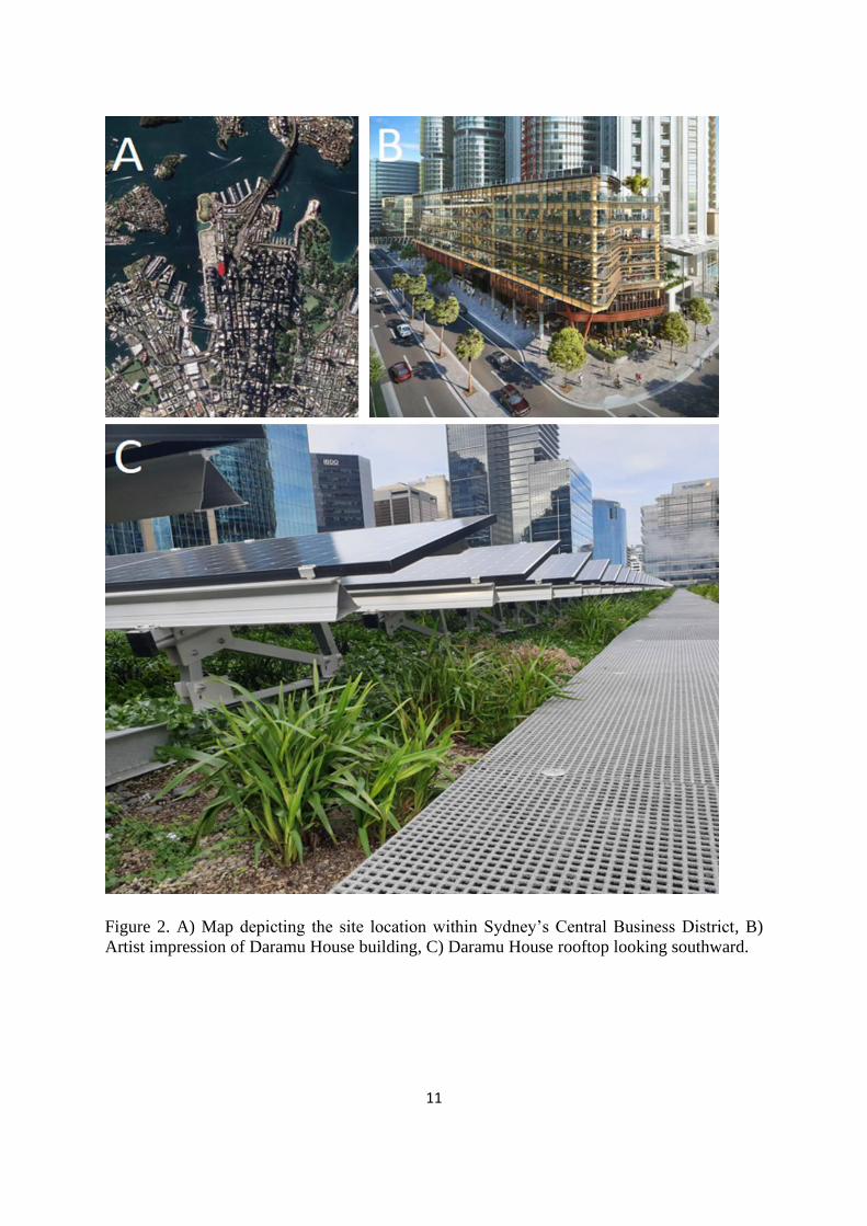
1.1 Site description

This study was conducted on two adjacent roofs atop recently constructed buildings in

Barangaroo, Sydney (-33.86479674708204, 151.20218101793557). Sydney has a humid

subtropical climate, receiving 1,309 mm of rain annually. Barangaroo is located on the north-

western edge of the Sydney Central Business District, bounded by Sydney Harbour to the

10

west, Barangaroo Central and Headland Park to the north, the Sydney Harbour Bridge

approach and northern Central Business District (CBD) to the east, and a range of new

development dominated by large CBD commercial tenants to the south.

The green roof on Daramu house was completed by Junglefy in September 2019, with the

onset of the spring season. Both the green and conventional roofs were 1,863.35 m2, with

593.96 m2 and 567.44 m2 PV panel coverages, respectively. The green roof employs a

planted area of 1,460.7 m2 (78.4% of the total roof space), with PV panels covering 40.66 %

of the planted areas. The combination of a green roof with PV panels is known as a Biosolar

roof. The study green roof was planted with a selection of native grasses and herbaceous

plants (Table 2). The native plant assemblages were selected to attract a diverse faunal

community to the roof. The studied green roof was constructed in 2019 and is an extensive

green roof, with a substrate depth of 120 mm and an integrated irrigation system. Extensive

green roofs have lower capital costs and building weight requirements than other green roof

types. As such, extensive green roofs are the most common around the world.

Figure 1. A) Daramu House green roof, view from Barangaroo Tower 1 and B) International

House rooftop looking southward.

11

Figure 2. A) Map depicting the site location within Sydney’s Central Business District, B)

Artist impression of Daramu House building, C) Daramu House rooftop looking southward.

12

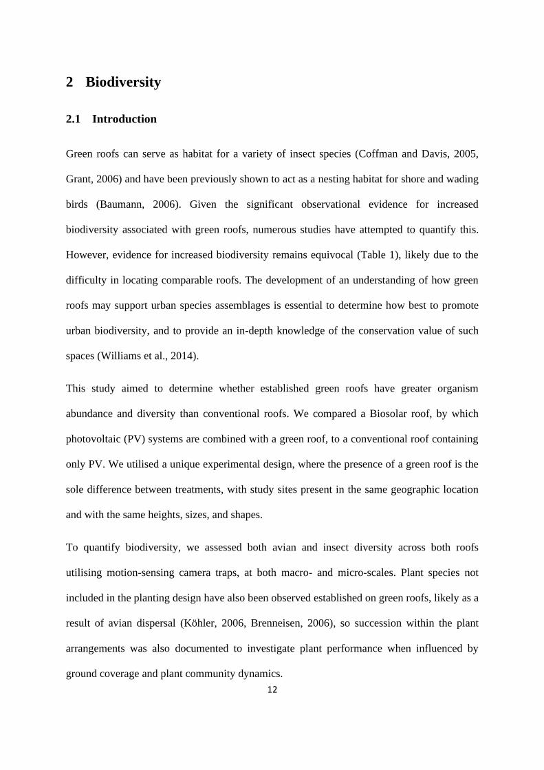
2 Biodiversity

2.1 Introduction

Green roofs can serve as habitat for a variety of insect species (Coffman and Davis, 2005,

Grant, 2006) and have been previously shown to act as a nesting habitat for shore and wading

birds (Baumann, 2006). Given the significant observational evidence for increased

biodiversity associated with green roofs, numerous studies have attempted to quantify this.

However, evidence for increased biodiversity remains equivocal (Table 1), likely due to the

difficulty in locating comparable roofs. The development of an understanding of how green

roofs may support urban species assemblages is essential to determine how best to promote

urban biodiversity, and to provide an in-depth knowledge of the conservation value of such

spaces (Williams et al., 2014).

This study aimed to determine whether established green roofs have greater organism

abundance and diversity than conventional roofs. We compared a Biosolar roof, by which

photovoltaic (PV) systems are combined with a green roof, to a conventional roof containing

only PV. We utilised a unique experimental design, where the presence of a green roof is the

sole difference between treatments, with study sites present in the same geographic location

and with the same heights, sizes, and shapes.

To quantify biodiversity, we assessed both avian and insect diversity across both roofs

utilising motion-sensing camera traps, at both macro- and micro-scales. Plant species not

included in the planting design have also been observed established on green roofs, likely as a

result of avian dispersal (Köhler, 2006, Brenneisen, 2006), so succession within the plant

arrangements was also documented to investigate plant performance when influenced by

ground coverage and plant community dynamics.

13

Table 1: Previously published literature on the biodiversity benefits of green roofs across

several countries with varying climates and comparison types.

Study Country Target

Organisms

Comparison Metric Results

(Williams et al.,

2014) Australia

Review – 20

papers

Green roofs &

ground level green

spaces

Hypothesis testing

Roofs can support similar

biodiversity to ground-level

habitats.

(MacIvor &

Lundholm, 2011) Canada Bees

Height of green roof Nest Success Height negatively impacted green

roof nest success.

(Pearce & Walters,

2012) England Bats

Roof type Bat calls More calls on green roof.

(Baumann, 2006) Switzerland Birds N/A Presence/Absence Organism present ✓

(Grant, 2006) England Birds N/A Presence/Absence Organism present ✓

(Berthon et al.,

2015) Australia Insects

Roof type Diversity 2x Abundance

3x Diversity

(Dromgold et al.,

2020) Australia Insects

Green roof & ground

level green spaces

Diversity Abundance and Richness higher

on ground-level habitats.

(Wang et al., 2017) Singapore Birds/Butterflies Roof type Presence/Absence Organism present ✓

(Pétremand et al.,

2017) Switzerland Beetles

N/A Presence/Absence Organism present ✓

2.2 Methods

2.2.1 Biodiversity monitoring

From August 2020 to June 2021, avian and insect communities visiting the green and

conventional roofs were monitored. To document biodiversity and organism activity, motion-

sensing camera trap arrays (Strike Force Pro XD, Browning USA) were established on both

roofs. Each roof featured a mirrored design, consisting of four cameras monitoring the

entirety of each roof. A non-invasive, camera trap approach was utilised so as to not interfere

with, reduce, or harm the faunal community on either roof. Cameras were set to capture a

single image when motion was detected, with a 1-second interval before retriggering.

Cameras were set up to focus on the predicted biodiversity hot spots on the green roof (e.g.

locations with dense vegetation), with their location mirrored on the conventional roof. Due

14

to the requirement that the plants do not cover the PV panels, plant height could not be

utilised as a measure of growth for rooftop plant species.

On each roof, a single “bee hotel” (Native Bee Sanctuary kit, Mr. Fothergill, Australia) was

strategically deployed and monitored using the camera array. Bee hotels were incorporated in

the experimental trial as the green roof design incorporated a native bee resting place, as well

as bee watering areas. Unfortunately, the previously established bee infrastructure on the

green roof could not be replicated on the conventional roof, so supplementary bee hotels were

employed.

Monitoring insect biodiversity with camera traps is challenging due to the size of many

insects and the image resolution capacity of camera trap systems. Camera traps are limited in

their ability to sample arthropods on the micro-scale, as they require an animal to pass

directly by the lens, within the image capture timeframe. In some cases, the motion of the

insect will trigger image capture before the organism can pass over the lens. To address this,

an additional camera-trap was deployed directly facing the bee hotels on each roof to monitor

resting insect biodiversity. Bee hotel specific camera-traps utilised the previously mentioned

settings. Additionally, insect surveys were conducted each fortnight covering the four garden

beds of the green roof, and their mirrored locations on the conventional roof. This study

consisted of two 5-minute monitoring periods within each section for each roof, with insect

species either photographed or noted down.

2.2.2 Data analysis

To compare insect and avian diversity between green and conventional roofs, avian and

insect richness and abundance data were used to calculate the Simpson’s diversity index and

the Shannon-Wiener index. All metrics were calculated both with avian and insect species

15

combined and separately to determine dissimilarities between taxon assemblages between the

green and conventional roofs. Diversity and richness metrics were calculated using the

‘vegan’ package in R (Version 3.6.3; R Core Team, 2020; Oksanen et al. 2020).

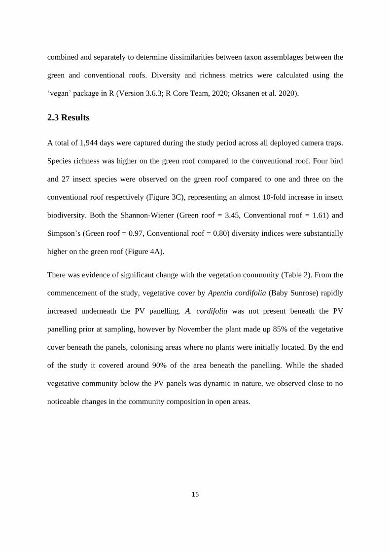
2.3 Results

A total of 1,944 days were captured during the study period across all deployed camera traps.

Species richness was higher on the green roof compared to the conventional roof. Four bird

and 27 insect species were observed on the green roof compared to one and three on the

conventional roof respectively (Figure 3C), representing an almost 10-fold increase in insect

biodiversity. Both the Shannon-Wiener (Green roof = 3.45, Conventional roof = 1.61) and

Simpson’s (Green roof = 0.97, Conventional roof = 0.80) diversity indices were substantially

higher on the green roof (Figure 4A).

There was evidence of significant change with the vegetation community (Table 2). From the

commencement of the study, vegetative cover by Apentia cordifolia (Baby Sunrose) rapidly

increased underneath the PV panelling. A. cordifolia was not present beneath the PV

panelling prior at sampling, however by November the plant made up 85% of the vegetative

cover beneath the panels, colonising areas where no plants were initially located. By the end

of the study it covered around 90% of the area beneath the panelling. While the shaded

vegetative community below the PV panels was dynamic in nature, we observed close to no

noticeable changes in the community composition in open areas.

16

Figure 3 A) Images of the four major vegetative sections of the green roof; B) Camera-trap

image of the conventional roof; C) Avian and insect community richness atop the green and

conventional roofs.

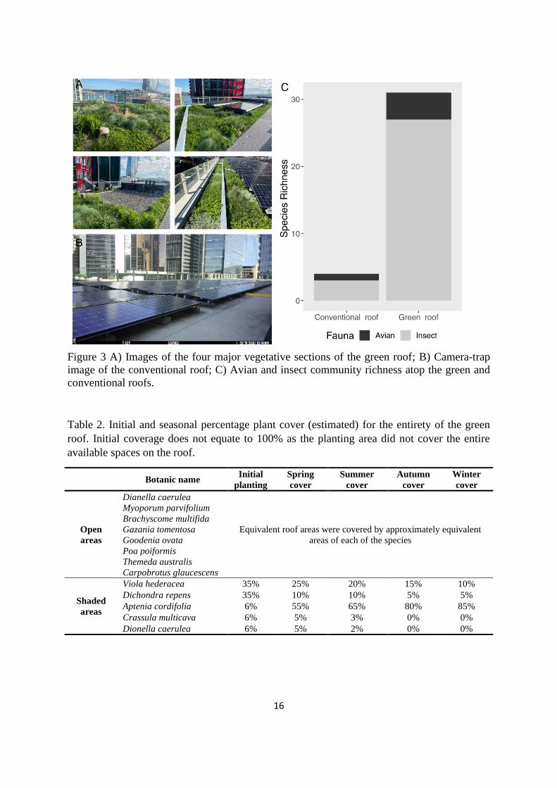
Table 2. Initial and seasonal percentage plant cover (estimated) for the entirety of the green

roof. Initial coverage does not equate to 100% as the planting area did not cover the entire

available spaces on the roof.

Botanic name

Initial

planting

Spring

cover

Summer

cover

Autumn

cover

Winter

cover

Open

areas

Dianella caerulea

Equivalent roof areas were covered by approximately equivalent

areas of each of the species

Myoporum parvifolium

Brachyscome multifida

Gazania tomentosa

Goodenia ovata

Poa poiformis

Themeda australis

Carpobrotus glaucescens

Shaded

areas

Viola hederacea 35% 25% 20% 15% 10%

Dichondra repens 35% 10% 10% 5% 5%

Aptenia cordifolia 6% 55% 65% 80% 85%

Crassula multicava 6% 5% 3% 0% 0%

Dionella caerulea 6% 5% 2% 0% 0%

17

Figure 4 A) Shannon-Weiner Diversity Index for combined avian and insect communities

atop the green and conventional roofs; B) Examples of faunal diversity – Blue Banded Bee

(Amegilla Cingulata), Spotted Dove (Spilopelia chinensis), Lychee metallic shield bug

(Scutiphora pedicellata), juvenile Pied Currawong (Strepera graculina), Australian Raven

(Corvus coronoides), Garden Snail (Cantareus aspersus), Spotted Dove (Spilopelia

chinensis).

18

2.4 Findings

The findings of this unique case study clearly demonstrate the biodiversity benefits of green

roofs in urban spaces. The studied green roof was capable of supporting four times the avian,

and nine times the insect diversity when compared to the conventional roof. The green roof

supported an eclectic (and probably highly dynamic) ecological community, providing refuge

to a conglomerate of native species. Further, there is evidence to suggest a significant pattern

in plant succession post construction in the shaded areas of the green roof. Extensive green

roofs can take up to two years to become established, thus the rapid plant succession over the

8-month monitoring period is likely to represent the climax plant population, as at the time of

project completion the green roof was 2 years old. This is essential as the shaded, below-

panel areas of a green roof are often the hardest to plan and maintain. The widespread

adoption of green roof initiatives, as a key component of the widespread promotion of urban

green space initiatives, will undoubtedly contribute significantly to a holistic and more

biologically diverse city space, providing refuge to rare and common species alike.

19

3 Air quality

3.1 Introduction

3.1.1 Air pollution and green roofs

There are three major mechanisms by which pollutants can be removed from the atmosphere:

dry deposition, wet deposition, and chemical reactions (Zannetti, 1990; Rasmussen, Taheri &

Kabel, 1975). Dry deposition refers to the gravimetric interception, impactions and

sedimentation processes by which particles are removed from the atmosphere. Wet deposition

refers to the transportation of pollutants by rain. Alongside these and other associated

processes, chemical reactions can occur whereby pollutants are degraded or transformed into

other compounds.

Plants are capable of improving air quality in several ways. They remove gaseous pollutants

through their stomates, particulate matter with their leaves, organic compounds with plant

tissues or through the microbial activity in the soil (Kumar et al., 2019; Fleck et al., 2020a;

Fleck et al., 2020b). Plants are also capable of indirectly reducing air pollution by

transpiration cooling and providing shade which decreases surface temperature and

photochemical reactions during which ozone forms (Rowe, 2011). The deposition of solid

contaminants onto vegetation through dry or wet deposition is one of the major pollutant

removal mechanisms of green roofs, but this process also occurs on hard surfaces. Processes

isolated to vegetation-associated activity, however, include the removal of gaseous

contaminants through stomatal uptake during photosynthesis (Pourkhabbaz et al., 2010), and

particles can be captured and retained in the complex plant substrate (Fleck et al., 2020b),

both sequestering the pollutants and preventing additional loading on stormwater systems.

20

The phytoremediation potential of green spaces is largely due to the various physiological

properties of the plant species present. Local climate is also an important factor that

influences the rates in which pollutants can be removed from the air. A warmer climate is

generally associated with an increased outdoor phytoremediation potential of green spaces

(Zhang et al., 2021). While trees found at ground level play a much larger role in pollution

abatement (Rowe, 2011), rooftops often comprise a significant proportion of impermeable

areas in urban settings, thus the installation of green roofs can drastically increase the green

coverage of metropolitan spaces. Despite this, there is limited evidence that green roofs may

improve urban air quality, and there is certainly no extensive research available in Australia

that quantitatively confirms this effect, or utilises direct comparisons with other urban

structures.

3.1.2 Quantifying air pollution removal by green roofs

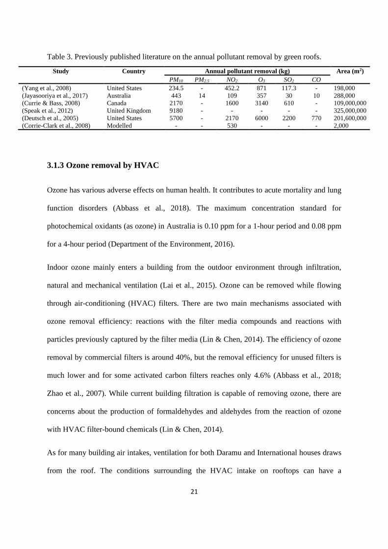
While the literature is limited, there are a number of studies that demonstrate the influence of

green roofs on air pollution mitigation, although the reported efficiencies vary (Table 3).

Plants are capable of phytoremediating air pollutants such as nitrogen oxides (NOx), sulphur

oxides (SOx), ozone (O3) and carbon monoxide (CO) during normal carbon dioxide (CO2)

uptake during photosynthesis.

It has been calculated that one square meter of green roof can offset the annual particulate

matter (PM) emissions of a single vehicle, driven 16,000 kilometres/year at 6.2 mg of PM for

every kilometre (Rowe, 2011). A scenario involving flat roofs in Manchester city showed that

green roofs could remove 0.21 tonnes of PM10 per year, equating to ~ 2.3 % of the PM10

observed in the area (Speak, 2013).

21

Table 3. Previously published literature on the annual pollutant removal by green roofs.

Study Country Annual pollutant removal (kg) Area (m2)

PM10 PM2.5 NO2 O3 SO2 CO

(Yang et al., 2008) United States 234.5 - 452.2 871 117.3 - 198,000

(Jayasooriya et al., 2017) Australia 443 14 109 357 30 10 288,000

(Currie & Bass, 2008) Canada 2170 - 1600 3140 610 - 109,000,000

(Speak et al., 2012) United Kingdom 9180 - - - - - 325,000,000

(Deutsch et al., 2005) United States 5700 - 2170 6000 2200 770 201,600,000

(Corrie-Clark et al., 2008) Modelled - - 530 - - - 2,000

3.1.3 Ozone removal by HVAC

Ozone has various adverse effects on human health. It contributes to acute mortality and lung

function disorders (Abbass et al., 2018). The maximum concentration standard for

photochemical oxidants (as ozone) in Australia is 0.10 ppm for a 1-hour period and 0.08 ppm

for a 4-hour period (Department of the Environment, 2016).

Indoor ozone mainly enters a building from the outdoor environment through infiltration,

natural and mechanical ventilation (Lai et al., 2015). Ozone can be removed while flowing

through air-conditioning (HVAC) filters. There are two main mechanisms associated with

ozone removal efficiency: reactions with the filter media compounds and reactions with

particles previously captured by the filter media (Lin & Chen, 2014). The efficiency of ozone

removal by commercial filters is around 40%, but the removal efficiency for unused filters is

much lower and for some activated carbon filters reaches only 4.6% (Abbass et al., 2018;

Zhao et al., 2007). While current building filtration is capable of removing ozone, there are

concerns about the production of formaldehydes and aldehydes from the reaction of ozone

with HVAC filter-bound chemicals (Lin & Chen, 2014).

As for many building air intakes, ventilation for both Daramu and International houses draws

from the roof. The conditions surrounding the HVAC intake on rooftops can have a

22

significant impact on the pollutant load brought indoors (Abbass et al., 2018). Under high

ambient ozone loads, there are concerns for the penetration of harmful chemicals into the

indoor environment. However, green infrastructure is capable of reducing ozone pollution

through stomatal uptake.

3.2 Methods

3.2.1 Ambient Air Quality monitoring

Two air quality sensor networks (AQY1, Aeroqual, New Zealand) were deployed on both the

green and conventional roofs. Each air quality sensor recorded PM2.5, O3 and NO2 on a 1-

minute timescale, which was transformed to 5-minute averaging periods for analysis.

Unfortunately, due to limited access to power on the rooftop, sensors could only be deployed

within range of the power supply (Figure 5.A). Sensors were treated as instrumental

duplicates to reduce instrument specific noise. Unfortunately, due to power loss, sensor

failures, and technical difficulties, some air quality data is missing from the presented results,

however 1,696,000 individual measurements were recorded across the four sensors, allowing

for meaningful comparisons to be made.

Portable weather stations (HP2551, Ecowitt, USA) were installed on each roof to record local

meteorological data. Additionally, BOM station #066214, located at Observatory Hill Park (~

600 m from the green roof), was also used to confirm weather parameters.

23

Figure 5. A) location of the AQY1s; B) Research Engineer Robert Fleck installing the

weather station.

24

3.2.2 Big-leaf resistance model

Dry deposition of air pollution was estimated using a big-leaf resistance model. The amount

of air pollutant (Q) that was removed from a certain area over a certain period of time (T) is

calculated using the formula (Nowak, 1994; Yang et al., 2008):

Q = F ∗ L ∗ T,

Where:

F – Pollutant flux 𝑔

𝑚2𝑠

L – Total area of green roof (m2)

T – Time

The pollutant flux was calculated using the formula (Nowak et al., 2006):

F = 𝑉𝑑 ∗ 𝐶 ∗ 10−8,

Where:

Vd – dry deposition velocity of an air pollutant (cm/s)

C – pollutant concentration in the air (µg/m3)

Dry deposition velocity takes into account aerodynamic resistance, quasi-laminar boundary

layer and canopy resistance (Yang et al., 2008). The dry depositional value varies depending

on the type of vegetation, amount of precipitation (as precipitation reduces removal rate via

dry deposition) and meteorological variables (Nowak et al., 2006; Yang et al., 2008).

Depositional velocities for different types of vegetation from (Yang et al., 2008) that were

similar to green roof vegetation are presented in the Table 4.

25

Table 4. Depositional velocities of NO2, O3 and PM relevant to the plants on the studied

green roof (Yang et al. 2008).

Study Pollutants Vegetation Vd Value (cm/s)

(Coe & Callagher, 1992)

Hesterberg et al., 1996)

NO2 Heathland

Grassland

0.10 – 0.35

0.11 – 0.24

(Stocker et al., 1993)

(Pio et al., 2000)

O3 Grassland (0.22 m)

Grass (0.1 – 0.8 m)

0.22 – 0.36

0.1 – 0.5

(Wesely, 1989)

(Fowler et al., 2004)

PM Nature grass (0.3-0.5 m)

Urban grass (0.1 – 0.25 m)

0.22 ± 0.06

0.33 – 0.38

3.3 Results

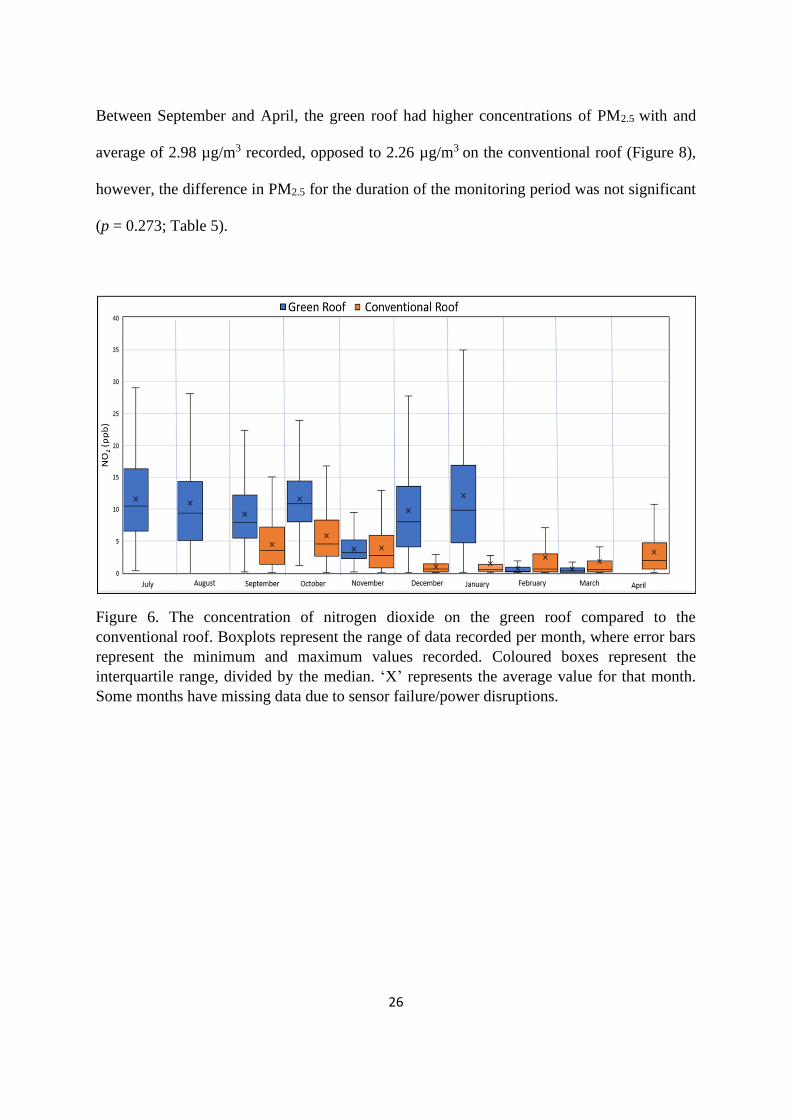
The average monthly air quality results between September 2020 and April 2021 are shown

in Figures 6-8.

Between September and January, nitrogen dioxide (NO2) concentrations were ~2.4 times

higher on the green roof than the conventional roof, with average concentrations of 9.46 and

3.88 ppb, respectively. However, during the months of February and March, NO2 on the

green roof was 2.2 times lower than the conventional roof (1.25 and 2.75 ppb respectively:

Figure 6). For the duration of the monitoring period, the NO2 observed on the green roof was

significantly higher than on the conventional roof (p = 0.02; Table 5). Inversely, Ozone (O3)

did not demonstrate the same degree of variability over the monitoring period. Between

September and March, O3 concentrations on the green roof were ~0.17 times lower than the

conventional roof (22.84 and 26.63 ppb respectively), with a maximum observed O3

concentrations of 29.5 and 39.5 ppb, respectively (Figure 7). The green roof presented

significantly lower concentrations of O3 for the comparable months (p = 0.000; Table 5).

26

Between September and April, the green roof had higher concentrations of PM2.5 with and

average of 2.98 µg/m3 recorded, opposed to 2.26 µg/m3 on the conventional roof (Figure 8),

however, the difference in PM2.5 for the duration of the monitoring period was not significant

(p = 0.273; Table 5).

Figure 6. The concentration of nitrogen dioxide on the green roof compared to the

conventional roof. Boxplots represent the range of data recorded per month, where error bars

represent the minimum and maximum values recorded. Coloured boxes represent the

interquartile range, divided by the median. ‘X’ represents the average value for that month.

Some months have missing data due to sensor failure/power disruptions.

27

Figure 7. The concentration of ozone on the green roof compared to the conventional roof.

Boxplots represent the range of data recorded per month, where error bars represent the

minimum and maximum values recorded. Coloured boxes represent the interquartile range,

divided by the median. ‘X’ represents the average value for that month. Some months have

missing data due to sensor failure/power disruptions.

Figure 8. The concentration of PM2.5 on the green roof compared to the conventional roof.

Boxplots represent the range of data recorded per month, where error bars represent the

minimum and maximum values recorded. Coloured boxes represent the interquartile range,

divided by the median. ‘X’ represents the average value for that month. Some months have

missing data due to sensor failure/power disruptions.

28

Table 5. Average observed pollutant concentrations. Statistical significance is denoted with *

at α = 0.05.

NO2 (ppb) O3 (ppb) PM2.5 (µg/m³)

Green roof 8.09 22.38 2.98

Conventional roof 3.61 26.24 2.26

Difference 4.48 -3.86 0.72

p-value 0.02* 0.00* 0.27

The National Environmental Protection Measures (NEPM, 2016) for ambient air quality is

shown in Table 6. During the time of measurements, maximum concentration standards were

not exceeded for NO2 and O3 and recorded measurements were much lower than the

standards. Similarly, there was no period where the standards for PM2.5 were breached.

Table 6. Standards for air pollutants (NEPM, 2016).

Pollutant Period Max conc. std Max allowable exceedances

NO2 (ppm) 1 hr

1 yr

0.12

0.03

1 day per year

None

O3 (ppm) 1 hr

4 hrs

0.10

0.08

1 day per year

1 day per year

PM2.5 (µg/m3) 1 day

1 yr

25

8

None

None

Upon commencement of the project, a large-scale construction site was being established in

the vicinity of the two buildings. During the early months, the site was underground and had

minimal impact on air pollution levels. However, from January to April, the construction

moved above ground and increases in PM2.5 were observed. During these months, a North-

29

West wind prevailed in Sydney (Figure 9), and as a result, there were elevated PM2.5

concentrations in the vicinity of the two roofs.

Figure 9. Left image; Green and Conventional roof positions in relation to nearby

construction including prevailing winds for the Sydney region for the monitoring period.

Right image; highlights the proximity and size of the construction project in relation to the

green roof.

3.3.1 Air pollution removal by the green roof

The big-leaf resistance model was used to estimate the pollutant removal potential of the

green roof (Table 7). Approximate dry deposition velocities (Vd) were taken from the

literature (Table 4) as 0.2 cm/s for NO2, 0.27 cm/s for O3 and 0.3 cm/s for PM. The recorded

average values of NO2 and O3 were converted to µg/m3, where 1 ppb is equal to 1.88 and 2.0

µg/m3, respectively.

30

Table 7. Big-leaf resistance model for the approximate annual removal rate of NO2, O3 and

PM2.5 for the green roof.

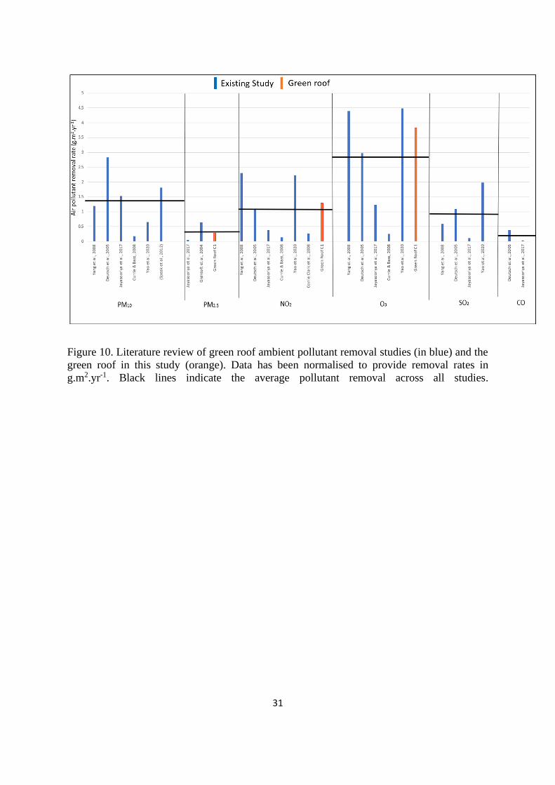
A review of the literature for the pollution removal rates of green roofs can be seen in Figure

10. On average, the pollutant removal rates for NO2, O3 and PM2.5 are 1.1, 2.86 and 0.33

g.m2.yr-1. Comparatively, the removal rates for NO2 and O3 presented here were 1.17 and

1.34 times greater than the average removal rates from the literature. However, the PM2.5

removal rates were only 0.87 times as effective as the average from the literature. While these

results are promising, the values reported here fall within the range of data provided in the

literature and the green roof from this project is performing within the expected ranges for all

pollutants. Variance in removal rates may be due to differing pollutant loading in the ambient

environment, meteorological conditions, seasonal variance and type of vegetation (Nowak et

al., 2006, Yang et al., 2008). While they were not recorded in this study, green roofs are also

capable of removing CO and SO2, as well as other size fractions of PM (eg. PM10). Based on

the literature presented below, it is expected that the green roof should be capable of

removing an average of 0.21, 0.94 and 1.36 g.m2.yr-1 of CO, SO2 and PM10.

Parameter NO2 O3 PM2.5

Annual removal rate, (g.m2.yr-1)

1.29

3.82

0.29

Air pollutant removal (kg)

2.3

6.9

0.5

31

Figure 10. Literature review of green roof ambient pollutant removal studies (in blue) and the

green roof in this study (orange). Data has been normalised to provide removal rates in

g.m2.yr-1. Black lines indicate the average pollutant removal across all studies.

32

3.4 Findings

NO2 detected on the green roof was ~2.4 times higher than the conventional roof, however

O3 was 0.17 times lower (p = 0.02 and 0.00, respectively). The reasons for these differences

in the NO2 concentrations are cryptic, however the net reduction O3 is often associated with

green infrastructure and was expected. PM2.5 varied through time with the ongoing

construction, however there were no statistically significant differences detected between

the two buildings. As such, annual pollutant removal rates were calculated for the green roof

based on plant foliage. This determined that the green roof would be able to remove 2.3, 6.9

and 0.5 kg.yr-1 of NO2, O3 and PM2.5, respectively. Removal rates for NO2 and O3 are better

than the average values reported in the literature, however PM2.5 removal is below average.

Each annual removal rate falls within the range of data provided by the literature, meaning

the Daramu House green roof is functioning within expectations for the removal of ambient

pollutant loads.

33

4 Thermal insulation

4.1 Introduction

Green roofs stabilise ambient temperatures and improve solar panel efficiency by creating

more suitable temperature conditions for energy production (Polo-Labarrios et al., 2020).

There is a correlation between the reliability and performance of PV panels and surrounding

ambient temperatures. As PV module surfaces heat up beyond optimal conditions, the panels’

efficiency decreases (Hoffmann and Koehl, 2014).

GRs lower ambient temperatures surrounding PV modules through evapotranspiration, in

turn, increasing PV system output (Shafique, Luo and Zuo, 2020). To date, most thermal

insulation studies have revolved around retrofitting rooftops with partial GR coverage, and

not providing comparisons with standard rooftops. There is very little research that compares

similar buildings which are exposed to similar environmental conditions by virtue of close

proximity.

The findings from this project will provide a more in depth understanding of integrated green

roofs within Sydney. No notable research projects of this kind in New South Wales, that have

two buildings in proximity with a similar size, climate, and age to contrast the thermal

properties of GI, have been previously performed. Due to a lack of previous research, there is

an absence of methodology for implementing this dual technology and quantifying the

benefits of green infrastructure in this climate.

34

4.2 Methods

4.2.1 Description and Temperature Sensors

From August 2020 to June 2021, 12 temperature loggers (i-Button model DS1921G,

Thermochron, USA; Figure 11) were employed to determine the vertical thermal gradient on

each roof (Figure 12). Each button recorded ambient temperature in 15-minute intervals for

up to 23 days. Buttons were collected and replaced fortnightly for ongoing data analysis.

There is a range of literature that describes the use of i-Buttons to collect thermal data on

green roofs in a range of climates (Fitchett, Govender and Wallabh, 2020, Lundholm, 2015).

Figure 11. i-Button temperature logger (DS1921G, Thermochron, USA) used in this study,

with protective FOB casing for impact protection.

i-Buttons were positioned in vertical alignment to determine the thermal gradient across the

roof layers. The i-Button positions are described below (Figure 12).

35

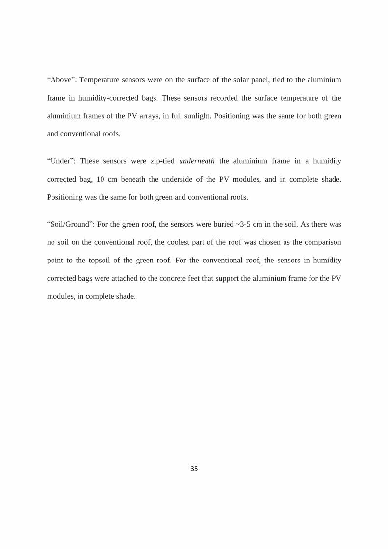
“Above”: Temperature sensors were on the surface of the solar panel, tied to the aluminium

frame in humidity-corrected bags. These sensors recorded the surface temperature of the

aluminium frames of the PV arrays, in full sunlight. Positioning was the same for both green

and conventional roofs.

“Under”: These sensors were zip-tied underneath the aluminium frame in a humidity

corrected bag, 10 cm beneath the underside of the PV modules, and in complete shade.

Positioning was the same for both green and conventional roofs.

“Soil/Ground”: For the green roof, the sensors were buried ~3-5 cm in the soil. As there was

no soil on the conventional roof, the coolest part of the roof was chosen as the comparison

point to the topsoil of the green roof. For the conventional roof, the sensors in humidity

corrected bags were attached to the concrete feet that support the aluminium frame for the PV

modules, in complete shade.

36

Figure 12. Temperature sensor vertical gradient positioning. “Above” sensors were

positioned in full sunlight on the aluminium frame supporting the panels. “Below” sensors

were positioned 10 cm below the panels. “Soil/Ground” sensors were positioned 3-5 cm

under the topsoil of the green roof and as far under the concrete footing of the conventional

roof as possible. Image is indicative of i-Button positions.

4.2.2 Thermal imagery camera

To monitor surface temperature fluctuations under varying environmental conditions, across

the range of materials used on both roofs, thermal imagery was employed (TG267, FLIR,

Australia). The images captured contain a thermal gradient displayed through variable

coloured imagery, as well as the surface temperature of the object in focus of the lens (Figure

13). Point transect sampling was employed along the length of each roof. At each sampling

point, six images were taken to comprise a sample representative of the rooftop. These six

images included a focus on: 1) single PV module surface temperature; 2) plant foliage/ground

immediately below single panel, shaded or unshaded; 3) walkway immediately in front of

37

plant foliage in direct sunlight, or ground in direct sunlight; 4) across the face of multiple PV

panels; 5) the gap between panels; 6) the plant foliage or ground immediately below the gap

between panels, only when in direct sunlight. If images were taken for one position in shaded

conditions, shaded conditions were replicated on the following roof using urban geometries at

a later time.

Figure 13. Examples of thermal imagery used on both green and conventional roofs. A)

temperature captured across the face of multiple panels in direct sunlight; B) temperature

captured between PV modules where exposed to sunlight and; C) surface temperature

captured of plant foliage in direct sunlight.

4.2.3 Thermal performance calculations

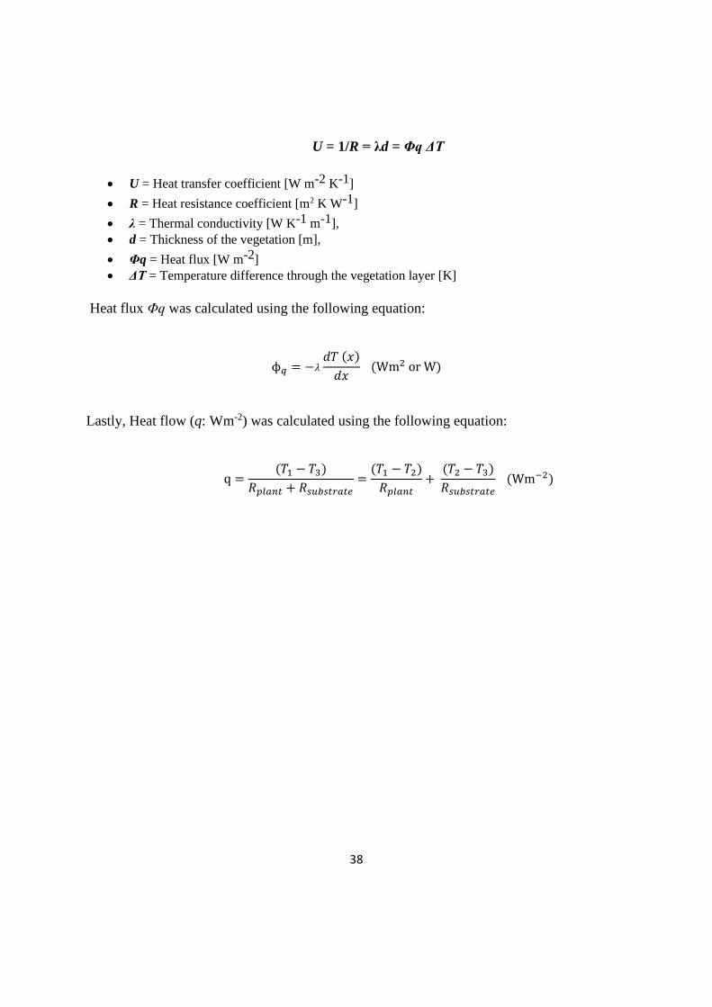
The insulation parameters of a green roof are expressed by the heat transfer coefficient (U),

the heat resistance coefficient (R), or the thermal conductivity (λ), which were determined by

the below equations. Additionally, values not recorded were sourced from the relevant

literature (Table 8).

38

U = 1/R = λd = Φq ΔT

• U = Heat transfer coefficient [W m-2 K-1]

• R = Heat resistance coefficient [m2 K W-1]

• λ = Thermal conductivity [W K-1 m-1],

• d = Thickness of the vegetation [m],

• Φq = Heat flux [W m-2]

• ΔT = Temperature difference through the vegetation layer [K]

Heat flux Φq was calculated using the following equation:

ϕ𝑞 = −𝜆 𝑑𝑇 (𝑥)

𝑑𝑥 (Wm2 or W)

Lastly, Heat flow (q: Wm-2) was calculated using the following equation:

q =(𝑇1 − 𝑇3)

𝑅𝑝𝑙𝑎𝑛𝑡 + 𝑅𝑠𝑢𝑏𝑠𝑡𝑟𝑎𝑡𝑒=

(𝑇1 − 𝑇2)

𝑅𝑝𝑙𝑎𝑛𝑡+

(𝑇2 − 𝑇3)

𝑅𝑠𝑢𝑏𝑠𝑡𝑟𝑎𝑡𝑒 (Wm−2)

39

Table 8. Review of the current literature relating to the thermal conductivity and thermal

resistance of plant species used in the construction of the green roof.

Study

Layers of Green roof

Thickness

d (m)

Thermal

Conductivity

λ [w/(mk)]

Thermal Resistance

Rc=d/λ [m2K W-1]

(Perini et al. 2011)

(Libessart & Kenai, 2018)

(Otelle & Perini, 2017a)

(Sudimac et al. 2018)

(Otelle & Perini, 2017a)

(Bianco et al. 2017)

(Bianco et al. 2017)

(Bianco et al. 2017)

(Otelle & Perini, 2017a)

(Otelle & Perini, 2017a)

(Otelle & Perini, 2017a)

(Moraue et al. 2012)

Vegetation Layer:

Viola hederacea

Dichondra repens

Crassula multicava

Aptenia cordifolia

Dianella caerulea

Myoporum parvifolium

Brachyscome multifida

Gazania tomentosa

Goodenia ovata

Poa poiformis ‘kingsdale’

Themeda australia ‘Mingo’

Carpobrotus glaucescens

0.1-0.15

1.67

0.5

0.12

0.05

0.14

0.56

0.56

0.56

0.12

0.14

0.14

0.79

0.09

0.3

1.3

3.2

1.1

0.27

0.27

0.27

1.3

1.1

1.1

0.19

(Abu-Hamdeh et al. 2001) Substrate (Slighted

compacted clay loam)

0.1-0.3 0.35 – 0.69 0.29 – 0.57 (d=0.2

m)

Concrete 0.14

4.3 Results and Findings

4.3.1 Thermal Performance - Theoretical

Comparisons between the average heat flux (q) in W.m2 for each roof, by month, can be seen

in Table 9. Due to seasonal trends and meteorological factors, monthly q was calculated to

determine the thermal energy transfer coefficient for the given time periods. In this case, a

higher q indicates a greater insulative effect for both heating and cooling. The findings of the

current work thus indicate that the green roof in this application could improve insulation for

the building against heat loss by several magnitudes, in some months.

40

Table 9. Calculated average, maximum and minimum heat flux (q; Wm-2) for both green and

conventional roofs, by month, accounting for rainfall as a co-variate.

October November December January February March April May

Green roof

Average q 3.027 4.03 3.55 4.47 3.75 3.78 4.15 2.81

Max. q 42.64 47.23 51.48 60.31 43.80 46.67 50.14 30.60

Min. q -18.23 -8.84 -7.88 -7.49 -6.92 -5.96 -8.26 2.81

Conventional roof

Average q 0.57 1.83 0.78 0.81 1.29 0.40 -0.04 0.44

Max. q 8.5 28.5 34 23.5 22 21 15.5 10.5

Min. q -1.5 -6.5 -5.5 -8.5 -5 -3.5 -4.5 -2

While the results presented here demonstrate a significant increase in the thermal insulation

of this commercial roofing application, there are several limitations to these calculations:

1) Temperature monitoring within the building was not performed due to confounding

variables such as HVAC use and building occupancy patterns affecting space usage

being beyond the researchers’ control. Therefore, these values are theoretical only.

2) These calculations do not consider the depth of the concrete roofing specific to each

site and are based on previously reported thermal resistance coefficients. Therefore,

these results pertain to the presence of a theoretical green roof under modelled

conditions.

4.3.2 Thermal Performance – Observed

Below is the observed vertical thermal gradient from the deployed temperature sensor

network. Paired comparisons are made between buildings represented by the green (green

41

roof) and black (conventional roof) lines. Vertical thermal gradients (“Above”, “Under” and

“Soil/Ground”) are represented by figure parts A, B and C, respectively.

Figure 14. Average daily temperatures across the green and conventional roofs detected from

i-Buttons: A) Above the PV; B) Below the PV; C) In the soil/at ground level. Green line =

Green roof, Black line = conventional roof. Red line indicates the change from Spring to

Summer, yellow line indicates the change from Summer to Autumn.

42

Figure 15. Maximum daily temperatures across the green and conventional roofs detected

from i-Buttons: A) Above the PV; B) Below the PV; C) In the soil/at ground level. Green line

= green roof, Black line = conventional roof. Red line indicates the change from Spring to

Summer, yellow line indicates the change from Summer to Autumn.

43

Figure 16. Minimum daily temperatures across the green and conventional roofs detected

from i-Buttons: A) Above the PV; B) Below the PV; C) In the soil/at ground level. Green line

= green roof, Black line = conventional roof. Red line indicates the change from Spring to

Summer, yellow line indicates the change from Summer to Autumn.

44

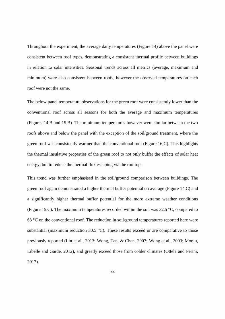
Throughout the experiment, the average daily temperatures (Figure 14) above the panel were

consistent between roof types, demonstrating a consistent thermal profile between buildings

in relation to solar intensities. Seasonal trends across all metrics (average, maximum and

minimum) were also consistent between roofs, however the observed temperatures on each

roof were not the same.

The below panel temperature observations for the green roof were consistently lower than the

conventional roof across all seasons for both the average and maximum temperatures

(Figures 14.B and 15.B). The minimum temperatures however were similar between the two

roofs above and below the panel with the exception of the soil/ground treatment, where the

green roof was consistently warmer than the conventional roof (Figure 16.C). This highlights

the thermal insulative properties of the green roof to not only buffer the effects of solar heat

energy, but to reduce the thermal flux escaping via the rooftop.

This trend was further emphasised in the soil/ground comparison between buildings. The

green roof again demonstrated a higher thermal buffer potential on average (Figure 14.C) and

a significantly higher thermal buffer potential for the more extreme weather conditions

(Figure 15.C). The maximum temperatures recorded within the soil was 32.5 °C, compared to

63 °C on the conventional roof. The reduction in soil/ground temperatures reported here were

substantial (maximum reduction 30.5 °C). These results exceed or are comparative to those

previously reported (Lin et al., 2013; Wong, Tan, & Chen, 2007; Wong et al., 2003; Morau,

Libelle and Garde, 2012), and greatly exceed those from colder climates (Ottelé and Perini,

2017).

45

This study has illustrated that a green roof can mitigate the high ambient temperatures

experienced in the Australian climate. Reductions in temperature were most pronounced in

comparisons between soil/ground temperatures. This is significant as rooftop cooling is an

important contributor to the reduction of Urban Heat Island effect, as well as building water

and energy consumption (Zhao et al., 2015).

It remains unclear if the thermal buffering potential below the solar panels is due to the

evapotranspiration effect of the plant foliage, or the physical layout of the solar panels (such

as height, tilt and azimuth), however, the specific design of the panels in this instance was

directly related to their integration with a green roof. To determine the precise contribution of

the plant foliage to reduced ambient temperatures above the soil layer would require a

purpose-built experimental system.

46

5 Stormwater Runoff

5.1 Introduction

Green Infrastructure, including green roofs, have been proposed as a system for managing the

increased stormwater runoff that has occurred as a result of urban development (Kalantari et

al., 2018). The green roof in this study was constructed with a proprietary growth substrate

(Junglefy P/L, Australia) which has specific properties which may have an impact on

stormwater runoff. The recorded effects presented here may not match those for green roofs

that use other media types with different properties, such as water holding capacity.

One of the objectives of green roofs is to manage surface water drainage holistically in line

with the ideals of sustainable development, by effectively managing runoff quantity, quality

and the associated amenity and biodiversity (Gregoire and Clausen, 2011). This can be

achieved by simulating the natural hydrological cycle, through a number of sequential

stormwater management interventions in the form of a treatment train. The components of

most green roofs; vegetation, substrate and storage layers as well as a drainage system, assist

in minimising peak flow during large storm events while also maintaining environmental

flow by storing and regulating the release of water over prolonged periods (Zheng et al.,

2021). The vegetation and substrate layers act together to capture water that is passed through

to the storage layer, which serves as a water reservoir in order to retain a portion of water,

while the excess is removed via the drainage system (Soulis et al., 2017). This is of particular

importance in dense urban environments following storm events, where peak runoff is

47

typically uncontrolled and regularly overwhelms stormwater drainage systems, resulting in

regular flooding (Sydney Water, 2015).

A study conducted by Mentens et al. (2006) found that the introduction of extensive green

roofs on a small percentage (10 %) of buildings can result in significant reductions in runoff;

54 % at the building level and 2.7 % at the city level as modelled on buildings in Brussels.

However, the actual performance of green roofs varies greatly depending on certain factors,

including rainfall, green roof coverage, soil medium, plant selection, the presence of

preceding dry periods and roof slope (Czemiel Berndtsson, 2010, Stovin et al., 2013, Zhang

et al., 2018). Results from Conn et al. (2020) reveal that there is a correlation between soil

thickness and water retention, and that this may change through time due to soil compaction

(Conn et al., 2020). Villareal and Bengtsson (2005) highlighted the effects of roof slope and

rainfall intensity on water retention, showing that a steeper slope and greater intensity of

rainfall both act to lower the performance and retention of a green roof.

Alongside field studies, many numerical models have also been developed in order to

understand the hydrological behaviour of green roofs under different conditions. For

example, Yang and Wang (2014) quantified the connection between green roof models and

parameter uncertainty through sensitivity analysis, and Sun et al. (2013) studied the effect of

solar radiation and medium layer moisture on hydrological performance.

Numerical modelling allows for greater quantification of results in a more consistent and

comparative manner by removing many of the uncertainties surrounding variables and

48

parameters, ultimately eliminating the constraint brought on by specific study locations (She

and Pang, 2010). Nonetheless, there is currently a lack research that confirms many of the

well understood (but often anecdotal) benefits of green roofs, especially with respect to

geographically relevant stormwater management. There are currently no known

demonstration research projects in Australia addressing these knowledge gaps.

This component of the project investigates:

• The efficacy of a green roof in reducing peak storm runoff.

• What is the potential for a green roof to mitigate pluvial flood flows in Sydney CBD?

• The potential for a green roof to mitigate stormwater pollution removal.

5.2 Materials and Methods

5.2.1 Flood study using DRAINS

The aim of the flood study was to describe the flood behaviour and flood hazard mitigation

capabilities of the green roof, under existing catchment conditions. For the purposes of this

research, the DRAINS hydrologic and hydraulic model was used to determine the

hydrological performance of the green roof acting as stormwater detention system. DRAINS

is a program used for designing and modelling stormwater in urban catchments and

incorporates methods from Australian Rainfall and Runoff. DRAINS is the main source of

hydrological design information in Australia. The program can be used to analyse peak flows,

volumes, and system deficiencies. DRAINS simulates the conversion of rainfall patterns to

49

stormwater runoff hydrographs and routes these through networks of pipes, channels and

streams.

For both the green and conventional roofs, the rooftop catchment was divided into four sub

catchments. These sub catchments were identified to represent uniform land use for which the

catchment characteristics of slope, impervious area and Manning’s roughness coefficient (n)

could be assumed constant. The division of the catchment was based on the building

hydrology design plans, drainage network information, aerial photography and the

information obtained from onsite field inspections.

The Hydrological Model used was DRAINS Australian Rainfall and Runoff 2019 Initial

Loss/Continuing Loss Model. Data was retrieved from the ARR Data Hub website using the

coordinates -33.861399, 151.201662. The impervious area initial loss was set at 1.5

(standard), and the impervious area continuing loss at 0. In order to correct the model for

suburban areas, as opposed to rural, the pervious area initial loss was corrected by a factor of

0.8, as per the ARR Data Hub specifications. Similarly, the pervious area continuing loss was

corrected by a factor of 0.4 x the value on Data Hub as per the DRAINS requirement for

conversion to a suburban area.

Historical rainfall data was sourced from ARR 2019 Storm from the Data Hub: Incremental

Pattern File and Intensity–Frequency–Duration Depth File. Pre burst rainfall data ie. storm

rainfall that occurs before the main rainfall burst, were retrieved for the coordinates -

33.861399, 151.201662. Major and minor storms with 5-minute to 2-hour durations were

50

selected (the design process defines the pipe sizes and depths needed to carry runoff from

minor storms satisfactorily, while meeting site specific criteria)

To model the conventional roof, a Pre-Development/Control Node was used to act as

comparison as a non-green roof/impervious surface, with the total area set to 1.8 ha, and

effective impervious area set at 100%. Further, the time of concentration for the effective

impervious area was assumed to be a minimum of 6-minutes according to ARR and

permeable area as 12-minutes as typical for grassed/pervious areas.

To model the green roof, the catchment area was divided into eight sections. Each catchment

area was taken from hydraulic engineering drawings, as per the building’s catchment plan.

Each catchment was assumed to be pervious, but this has its restrictions as the green roof is

“pervious” but with an impervious, finite waterproof base. Each catchment was directed into

a detention basin which was designed to represent the assumed 20 % void space in the green

roof substrate that can theoretically hold water when it rains. Note that 20 % of the depth was

taken to calibrate the 20 % volume of each catchment area. Since green roof filtration depth

was 0.15 m, 0.03 m was adopted for each detention basin node. The void space dimensions

were taken at 1.00 and 1.03 for ease of setting pipe inverts. A circular culvert was

incorporated, as the green roof drains to a circular pipe. K entry/K bends were set at 0.5.

Additionally, rectangular vertical sides were assumed on for the green roof. Outlet/underdrain

pipes were set at 150 mm in diameter, and the length of each pipe was taken as longest route

within each catchment to the outlet pit.

51

To model overflow routes, allowing accurate determination of water levels and flow

characteristics during large storm events, the following assumptions were made: 1) the

pathway was flat around green roof walls as the overflow route; 2) side length of 10 m; 3)

Weir coefficient set as C = 1.75 to reflect a sharp crested, vertical water face; 4) crest length

of 10 m to reflect longest green roof side in that catchment; 5) crest level at 1.03 which is

when 20 % void area is full of water and water ponds at the surface of the substrate; 6) the

percentage of downstream catchment flow carried by this channel was zero - to reflect that

surrounding catchment flow is all captured by its own overflow path and pipe system; 7)

channel slope = minimum 1 % grade; 8) safe parameters are typical for stormwater design –

Standards Australia 3500.3.

As it is difficult to incorporate details about pits with inflow and outflow data, a standard

NSW grated inlet pit was used which has inflows loaded from NSW data specifications. Two

catchments were directed to each pit, to represent the green roof area on each side of the

central path draining to their respective pit which then transfers water to the pipe under the

pathway and then onwards into the piped drainage system for the building before connection

into the Council system.

5.2.2 Model for Urban Stormwater Improvement Conceptualisation (MUSIC)

The Model for Urban Stormwater Improvement Conceptualisation (MUSIC) is a tool for

simulating urban stormwater systems for a range of catchment scales and applications.

MUSIC is particularly useful as conceptual design tool which allows for water quality

52

improvement assessment through modelling the simulated gross pollutant removal and flow

reduction through stormwater management systems such as constructed wetlands,

bioretention rain gardens, or in this case, the green roof. Using MUSIC, we have the ability to

simulate both quantity and quality of runoff from catchments and the effect of treatment

facilities on these components. MUSIC is an aid to decision making. It enables users to

evaluate conceptual designs of stormwater management systems to ensure they are

appropriate for their catchments. By simulating the performance of stormwater quality

improvement measures, MUSIC determines if proposed systems can meet specified water

quality objectives. MUSIC will simulate the performance of a group of stormwater

management measures, configured in series or in parallel to form a treatment train. MUSIC

runs on an event or continuous basis, allowing rigorous analysis of the merit of proposed

strategies over the short-term and long-term.

Specifically, the software enables users to:

• Determine the likely water quality emanating from urban catchments.

• Predict the likely performance of specific structural best management practices

(BMPs) in protecting receiving water quality.

• Design an integrated stormwater management scheme.

• Evaluate the success of structural BMPs, or a stormwater management scheme,

against a range of water quality standards.

Water quality improvements of the modelled technologies were based on the default trends

available in MUSIC. Potential WSUD strategies which could assist the ultimate objective of

53

runoff nutrient reduction are built into MUSIC, where the effectiveness of the strategies can

be assessed from allotment to catchment scale:

• Allotment scale – source control such as rainwater tanks, rain gardens and soakways

treating 25%, 50% and 75% of the catchment.

• Street scale – swales, bioretention systems and pervious pavements treating 25%,

50%, and 75% of the catchment.

• Catchment scale – infiltration basin (1000 m2) and Wetland (1000 m2).

Overall, the model provided comparable quality data for initial stormwater management

strategy assessment.

5.2.3 Elemental analysis

Trace metal analysis was conducted on composite samples collected on each roof. Samples

were collected each month, at two points on the roofs (north and south end) to determine the

trace metal profile. Green roof samples were collected by taking a 30 gram sample of the

substrate, and carefully removing any rocks or fertilizer pellets. Samples were collected

without the use of metal tools and stored in sterile falcon tubes (n = 2 per time point).

Conventional roof samples were collected using a Ryobi One+Hand Vacuum (18V, Ryobi,

Australia) and deposited into sterilised zip lock bags for transportation. Vacuum samples

were collected by vacuuming two composite areas, covering 1 m2 each, in triplicate (n = 2 per

time point). Samples were transported to UTS for storage until sample preparation.

54

Samples were dried in a drying oven at 65°C for 36 hours, and weighed and transferred to 50

mL falcon tubes and diluted with at least 45 mL of MilliQ water (Ω 18.2; Millipore,

Germany). Samples were sonicated using a water bath sonicator for 15-minutes to disrupt any

aggregated particles and ensure solubilisation of heavy metals. Samples were then

centrifuged at 4500 g to separate the particles from the water column, and the soluble fraction

was poured off into a fresh 50 mL falcon tube.

The insoluble fraction was then digested in 1:1 69% v/v nitric acid and 30% v/v hydrochloric

acid and made to volume with MilliQ to prepare for Solution Nebulization Induction Coupled

Plasma Mass Spectrometry (SN-ICP-MS; 7500cx, Agilent, USA). Samples were processed in

technical triplicate. A 12-point calibration curve was made from a 68 elemental standard set

(ICP-MS68A-500 Choice Analytical) in 2% HNO3 / 1% HCl diluent. The calibration points

were as follows: 5, 2.5, 1, 0.5, 0.25, 0.1, 0.05, 0.01, 0.005, 0.0025, 0.001, and 0 ppm.

Prior to analysis, samples were again digested in high purity nitric acid (15.6 M) in closed

vessels using a microwave apparatus (MARS Xpress, CEM) according to US EPA method

3051A. Analysis of the collected samples focused on particulate phosphorous and the sorbed

metals, primarily lead (Pb), zinc (Zn), copper (Cu), chromium (0) and Iron (Fe).

All SN-ICP-MS was performed using 7700x series ICP-MS (Agilent Technologies, USA)

equipped with a micromistTM concentric nebuliser (Glass Expansion, Australia). A Scott

type double pass spray chamber cooled to 2°C was used for sample introduction. Platinum

sampling and skimmer cones were used. The 7700x ICP-MS was controlled by Agilent

Technologies ICP-MS MassHunter 4.3 software (C.01.03) on a Hewlett-Packard (Hewlett-

55

Packard, USA) desktop computer via a category 5e ethernet cable. All experiments used

99.9995 % ultra-high purity liquid argon (Argon 5.0, Coregas Pty Ltd, Australia).

SN-ICP-MS was used to analyse the digested standards. An Agilent integrated autosampler

(AIS) was loaded with solutions for analysis (7700cx, Agilent, USA). Solutions were

transferred to the ICP-MS using a 1.02 mm internal diameter Tygon tubing and a three

channel peristaltic pump. The solution was pumped at a continuous flow of 1.0 mL.min-1. A

100 ppb Rhodium solution in 1% HNO3 was used as an internal standard and introduced into

the analyte flow via a T connector post-pump. The solution was delivered to the plasma of

the ICP via a Micromist nebulizer and Scott type double pass spray chamber. The typical

ICP-MS conditions can be found in Table 10.

Table 10. SN-ICP-MS (7700cx, Agilent, USA) parameters used for heavy metal analysis.

Agilent 7700cx SN-ICP-MS

Sample Introduction

RF power (W) 1500

Carrier gas flow rate (L.min-1) 0.7

Makeup gas flow rate (L.min-1) 0.5

Sample depth, mm 8

Ion lenses

Extracts 1,2 (V) 3.8,-185

Omega bias, lens (V) -120, 18

Cell entrance, exit (V) -30,-40

Octopole parameters

Octopole RF (V) 190

Octopole bias (V) -8

Collision gas, flow rate (mL.min-1) 0

56

5.2.4 StormWater Management Model (SWMM)

As outlined by Hicks et al. (2009), the availability of data describing the hydrologic response

of urban catchments is extremely limited. For this reason, a common approach is to generate

the data using catchment models. During these processes, there are three main sources of

variability that should be avoided, or otherwise acknowledged:

After considering a range of alternative modelling solutions (not presented in detail here), the

SWMM system (Rossman, 2015) was used for data generation. The SWMM model is well

credentialled for numerous uses in urban environments (Brady, 2015; Broekhuizen et al.,

2020; Sun, 2014; Zaghoul, 1983).

As the study site is relatively new, there is a lack of on-site catchment monitoring data.

Therefore, generated observational data from Observatory Hill, Sydney (Gauge 066062) was

used (Figure 17). Observatory Hill has continuous rainfall records from this location since

1913, so both short and long period simulations are feasible. While there is over 100 years of

data available, only the period from 1991 to 2010 was selected for this analysis. Additionally,

the evapotranspiration (ET) rate from the vegetative surfaces on the green roof is required for

SWMM analysis, which was set to a constant 3 mm per day. While the analysis conducted

can describe the collection and transport of stormwater for each roof type, changes in

hydrograph phasing within the city drainage infrastructure could not be determined with the

available data.

57

Figure 17. Proximity of Observatory Hill from the study site – approximate linear distance is

590 m.

58

Parameters for each roof are described in Table 11.

Table 11. Model parameters used to describe each roof for SWMM analysis.

Parameter Conventional roof Greenroof

Total catchment area 0.09 ha 0.09 ha

Impervious fraction 100 % 10 %

Green roof fraction N/A 90 %

Soil depth N/A 120 mm

Impervious depression storage 1 mm 1 mm

Roof slope 1.25 % 1.25 %

SWMM model analysis provided two potential metrics for assessing the minimisation of

anthropogenic impacts on hydrological fluxes through the effects provided by the green roof:

1) Flood flows – can the green roof reduce stormwater runoff, and what effect did it have

on surface ponding?

2) Runoff yield – can the green roof reduce the volume of water draining to the outlet.

59

5.3 Results & Findings

5.3.1 DRAINS modelling

Based on a once in a 5-year storm event (20% Annual Exceedance Probability; AEP), the top

water level was 1.04 m in each “detention basin”/green roof catchment area. Contextually,

this means that no water will spill over the side of the building unless it builds up to 1.05 m.

Outlet flow from the green roof under this AEP level is predicted to be 7 L/s compared to 634

L/s from the conventional roof, indicating the potential for a considerable reduction in net

stormwater runoff (Figures 18 and 19).

60

Figure 18. 20 AEP storm event run result from DRAINS modelling software. The detention

nodes (blue triangles and black numbers) represent the volume of water flowing across the

catchment area (m3/s); the green numbers represent the upper and lower water depths

described as cm above 1.0 (e.g. 1.03 = 3 cm); the red numbers denote the water overflow

over the edges of the roof, and the dark blue numbers represent the L/s of water flowing

through the green roof underdrain/pipe to the outlet pit.

61

Figure 19. 1 AEP storm event run result from DRAINS modelling software. The detention

nodes (blue triangles and black numbers) represent the volume of water flowing across the

catchment area (m3/s); the green numbers represent the upper and lower water depths

described as cm above 1.0 (e.g. 1.03 = 3 cm); the red numbers denote the water overflow

over the edges of the roof, and the dark blue numbers represent the L/s of water flowing

through the green roof underdrain/pipe to the outlet pit.

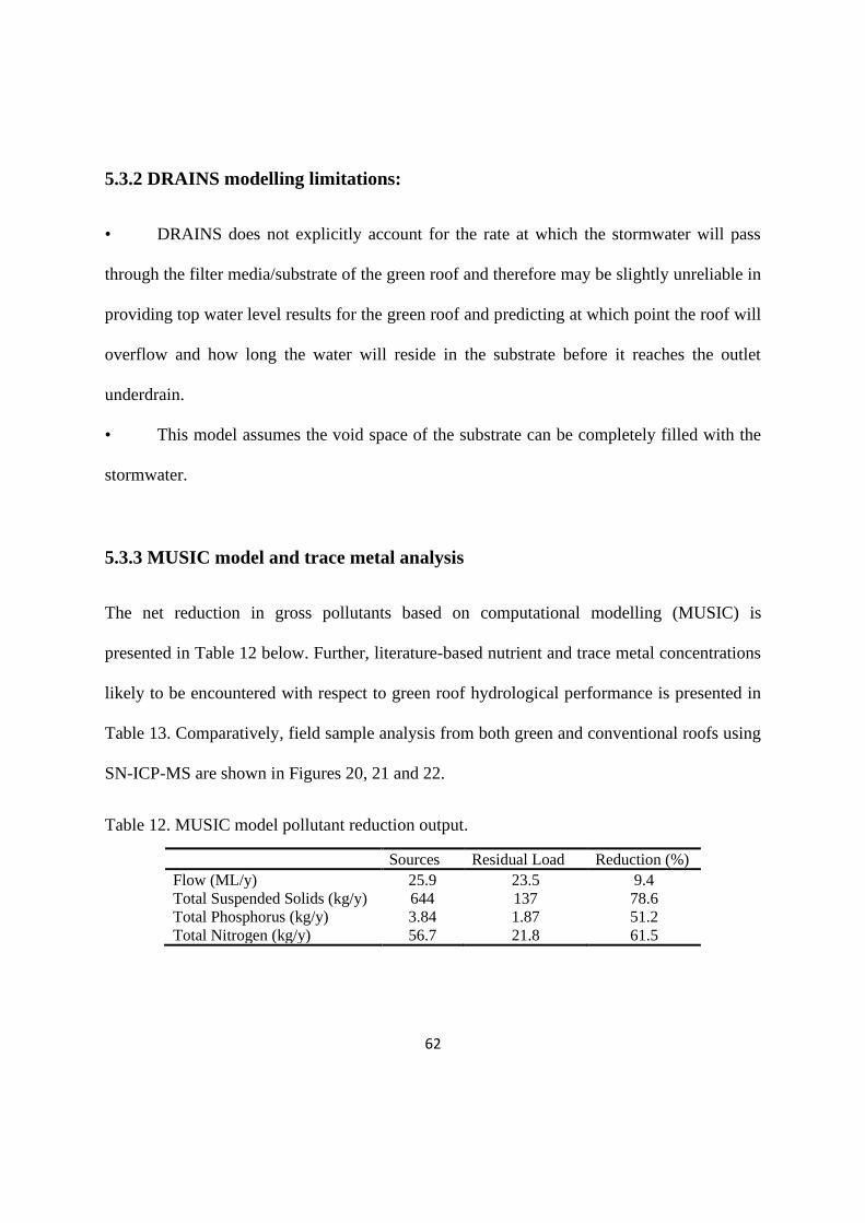
62

5.3.2 DRAINS modelling limitations:

• DRAINS does not explicitly account for the rate at which the stormwater will pass

through the filter media/substrate of the green roof and therefore may be slightly unreliable in

providing top water level results for the green roof and predicting at which point the roof will

overflow and how long the water will reside in the substrate before it reaches the outlet

underdrain.

• This model assumes the void space of the substrate can be completely filled with the

stormwater.

5.3.3 MUSIC model and trace metal analysis

The net reduction in gross pollutants based on computational modelling (MUSIC) is

presented in Table 12 below. Further, literature-based nutrient and trace metal concentrations

likely to be encountered with respect to green roof hydrological performance is presented in

Table 13. Comparatively, field sample analysis from both green and conventional roofs using

SN-ICP-MS are shown in Figures 20, 21 and 22.

Table 12. MUSIC model pollutant reduction output.

Sources Residual Load Reduction (%)

Flow (ML/y) 25.9 23.5 9.4

Total Suspended Solids (kg/y) 644 137 78.6

Total Phosphorus (kg/y) 3.84 1.87 51.2

Total Nitrogen (kg/y) 56.7 21.8 61.5

63

The MUSIC model established predicts substantial stormwater pollution removal rates for

suspended solids, phosphorus, and nitrates. However, it is important to note, while the

MUSIC model provides some insight into the potential reduction in various pollutants, the

model is primarily designed for streetscapes. While the model predicts a net reduction in

nutrients (phosphorus and nitrogen), the additional fertilisers used on the green roof have not

been accounted for. Nonetheless, the net flow and suspended solids reductions may still be

representative as a proportion received on a green roof.

Table 13. Examined literature relating to the bioretention of trace metals from stormwater and

impervious surfaces.

Study Investigation Location

(Davis et al. 2001) Laboratory experiment USA

(Davis et al. 2003) Laboratory experiment USA

(Hsieh & Davis 2005) Laboratory experiment USA

(Glass & Bissouma 2005) Field observations Washington DC, USA

(Sun & Davis 2007) Laboratory experiment USA

(Hunt et al. 2006) Field observations North Carolina, USA

(Roseen et al. 2006) Field observations New Hampshire, USA

(Davis 2007) Field observations Maryland, USA

(Hunt et al. 2008) Field observations North Carolina, USA

(Chapman & Horner 2010) Field observations Washing, USA

Following a review of the literature related to trace metal bioretention (Table 13), nutrient

and trace metal concentrations in surface accumulated dust and substrate were modelled for

both green and conventional roofs. The model (Figure 20) depicts the total sums of soluble

and insoluble nutrient and trace metal concentrations detected in these materials. While the

magnitude of the modelled results is substantially lower than those observed in this study, the

64

trend for trace metals is similar, indicating that both roofs are functioning within

expectations.

Figure 20. Modelled total nutrient and trace metal analysis for green and conventional roof

substrate and surface dust respectively. Nutrients are to the left of the black dashed line (blue

arrow) and trace metals to the right (red arrow). Error bars represent the SEM.

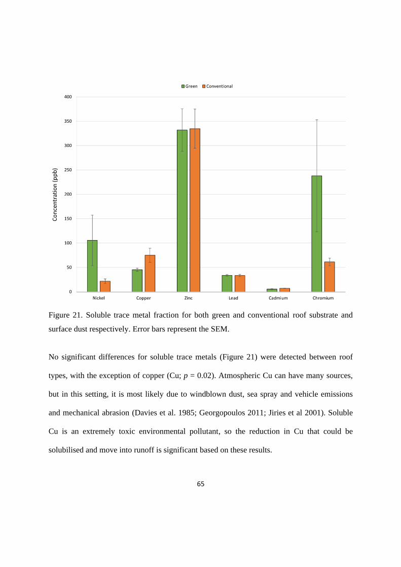
65

Figure 21. Soluble trace metal fraction for both green and conventional roof substrate and

surface dust respectively. Error bars represent the SEM.

No significant differences for soluble trace metals (Figure 21) were detected between roof

types, with the exception of copper (Cu; p = 0.02). Atmospheric Cu can have many sources,

but in this setting, it is most likely due to windblown dust, sea spray and vehicle emissions

and mechanical abrasion (Davies et al. 1985; Georgopoulos 2011; Jiries et al 2001). Soluble

Cu is an extremely toxic environmental pollutant, so the reduction in Cu that could be

solubilised and move into runoff is significant based on these results.

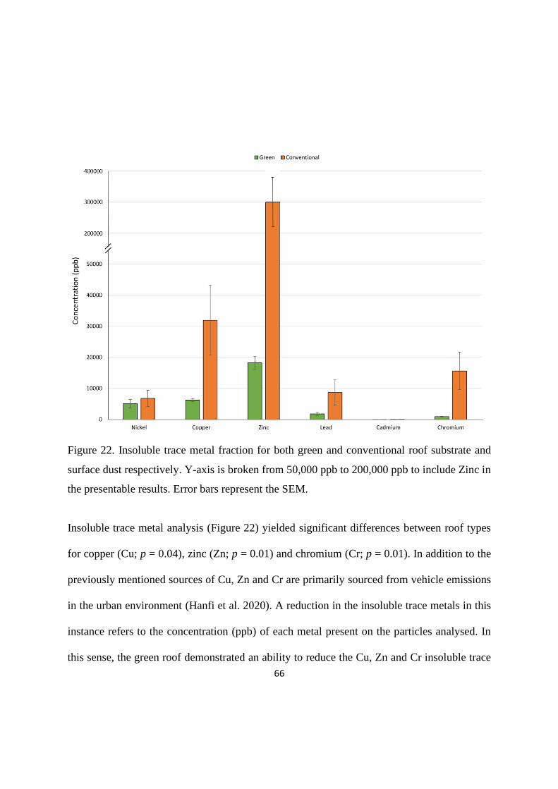
66

Figure 22. Insoluble trace metal fraction for both green and conventional roof substrate and

surface dust respectively. Y-axis is broken from 50,000 ppb to 200,000 ppb to include Zinc in

the presentable results. Error bars represent the SEM.

Insoluble trace metal analysis (Figure 22) yielded significant differences between roof types

for copper (Cu; p = 0.04), zinc (Zn; p = 0.01) and chromium (Cr; p = 0.01). In addition to the

previously mentioned sources of Cu, Zn and Cr are primarily sourced from vehicle emissions

in the urban environment (Hanfi et al. 2020). A reduction in the insoluble trace metals in this

instance refers to the concentration (ppb) of each metal present on the particles analysed. In

this sense, the green roof demonstrated an ability to reduce the Cu, Zn and Cr insoluble trace

67

metals bound to particles, or trapped in the plant substrate, through mechanisms unexplored

here. Further analysis should be conducted to determine the mechanism behind the reduction

in these specific metals to determine if the difference is due to the plant foliage, or the various

physiochemical properties of the substrate.

While the total trace metal concentrations detected on the two roofs in this study were

magnitudes higher than those modelled, the trace metal trends between the two buildings are

consistent. This indicates that there is a definite trend for green roofs to reduce certain trace

metals in their insoluble form, with comparable removal efficiencies to various industrial

filter materials (Reddy, Xie & Dastgheibi 2014). Further analysis on stormwater retention

time with substrate depth and reductions in soluble trace metal concentrations would

potentially yield more significant results than those presented here.

5.3.4 SWMM Analysis

Two characteristics of flood flows will be considered in this analysis, namely the theoretical

runoff under varying storm conditions from the green and conventional roofs, and the depth

of surface ponding. The estimation of these flood characteristics requires the determination of

the magnitude of the hazard, and its likelihood of occurrence, referred to as Annual

Exceedance Probability (AEP %).

68

The analysis conducted demonstrates a significant reduction in risk events more frequent than

5% AEP (i.e. 1 in 20-years; Figure 23). As expected, the physical properties of the green roof

reduced the design flow for a typical underground stormwater drainage network. It should be

noted (Figure 23), that there were six years where the annual maximum flow was low to zero.

As such, these years were censored from the frequency analysis, which has led to a greater

uncertainty associated with the risk profile for the green roof catchment. Considering this, the

assessment of the 1 in 100-year AEP design flow indicates there would be little or no

reduction in flood risk for these rare events.

If the current installation of an extensive green roof was to be considered as standard, further

analysis could be conducted on the efficacy of green roofs as a technology to reduce flood

flow for an entire urban centre. The current findings indicate that it is plausible that the

widespread adoption of extensive green roofs in the Sydney metropolitan area could

significantly reduce the flood flow of the underground stormwater management network.

69

Figure 23. Flood flow prediction model with upper and lower confidence limits for each roof

type based on storm event AEP.

Another metric for performance in relation to stormwater management is the change in runoff

yield. In an urban environment, many water quality impacts are influenced by the volume of

runoff. A reduction in runoff volume will reduce the transport capacity of potential

contaminants. For the two roofs considered, the average yearly rainfall was 980 mm (20-year

dataset). While there was little difference in modelled the volume of water transported from

the two roofs, there was a reduction in the peak flow rate arising from storage within the

70

green roof substrate. This outcome was a function of both the assumed characteristics of the

green roof, and the limited substrate depth of 120 mm. An increase in substrate depth would

increase the retention time and consequently increase both the uptake by vegetation and

removal by evaporation. To extend our capacity to understand the stormwater management

performance of green roofs like the one tested, further modelling using more comprehensive

green roof construction and cityscape data should be conducted.

71

6 PV performance assessment

6.1 Introduction

The installation of PV systems on city-scape rooftops is an integral technology to address the

growing need for renewable energy sources (Jahanfar et al., 2020). The Clean Energy

Council of Australia reports that the adoption of small-scale (up to 100 kW) PV systems has

increased 8-fold since 2010 (Clean Energy Australia, 2021), and this trend is likely to be

similar for commercial properties with larger systems. While green roofs (GR) are often

designed to be an aesthetic greenspace for building occupants, the opportunity to construct

green systems to operate as functional additions to building services is starting to gain

traction. There is mounting evidence to quantify the numerous benefits of GR installation,

amongst which PV energy outputs are of significant interest. The benefits of integrated GR-

PV (Biosolar) technologies are numerous, however, there are significant discrepancies

worldwide for the reported energy benefits of Biosolar arrays (-0.06 to 4.3%: Table 14).

Discrepancies appear to be closely aligned with geographical location and climate type, as

well as experimental design and building layout. It is therefore essential to make GR-PV

observations between buildings with similar characteristics, such as construction material,

size, and location.

72

Table 14: Previously published literature on the energy output benefits of Biosolar systems

across a range of climates and roof comparisons. Few studies utilise a multi-building design

and/or long-term monitoring.

Authors Study

Location Study Type

Time

period

PV output

Enhancement Climate Type Roof Type Comparisons

(Hui and Chan, 2011)

Hong Kong Experimental & Simulation

12 months 4.3% Subtropical PV-green vs PV-concrete

(Perez et al.,

2012)

New York

City, US

Experimental

& Simulation 10 months 2%

Humid

continental PV-green roof vs. PV gravel

(Chemisana and

Lamnatou,

2014)

Lleida,

Catalonia,

Spain

Experimental 5 days 1.29 (Gazania) 3.33% (Sedum)

Subtropical (Mediterranean)

PV-green vs. PV-gravel

(Osma et al.,

2016) Colombia Experimental - 1-2% Subtropical PV-green vs. PV-black

(Ogaili and

Sailor, 2016)

Portland,

Oregon, US Experimental 3 months 0.8-1.2%

Subtropical

(Mediterranean) PV-green vs. PV-black/white

(Alshayeb and

Chang, 2018) Kansas, US Experimental 12 months 1.4%

Humid

subtropical PV-green vs. PV-black

(Baumann et

al., 2019)

Winterthur,

Switzerland Experimental 5 months -0.06%

Warm humid

continental

Bifacial PV-green roof vs.

flat roof

6.2 Materials and Methods

Both the green and conventional roofs employed the use of four SolarEdge three phase

inverters (27.6k-AU000NNU2, SolarEdge, USA) rated to operate at a 98 % efficiency. The

green roof employed 335 SunPower MAXEON 3 panels (pNom 395W: efficiency 22.6 %),

with a total system size of 593.96 m2 and a peak nominal power of 132.33 kWp. The

conventional roof employs 346 LG NeON2 panels (pNom 320W: efficiency 19.5 %), with a

total system size of 567.44 m2, and a peak nominal power of 110.72 kWp. Each roof hosted a

suite of environmental sensors; a temperature sensor for ambient weather conditions,

pyranometer for local irradiance, and a weather station to record wind direction and speed.

Additionally, the system collects meteorological data from the Bureau of Meteorology, used

73

to cross-reference local weather conditions. All data was uploaded and managed through the

SolarEdge monitoring web-platform. Solar array energy outputs and environmental

conditions were downloaded and analysed fortnightly.

Obviously, photovoltaic energy generation hinges primarily on incident solar irradiance. As

such, a 3D model of the Barangaroo district was developed to estimate the average yearly

incident solar irradiance on each roof top (Figure 24) using the Rhino 6 modelling software,

and average annual solar radiation analysis was conducted using DAYSIM in Grasshopper’s

Honeybee plug-in. Solar radiation calculations were based off the Sydney CBD

Representative Meteorological Year (RMY) file (AUS_NSW.Sydney.947680, EnergyPlus).

The green and conventional roofs experience slightly different light exposure due to the

influence of the surrounding urban geometries on the day arc (shading), building light

reflectance, as well as differences in panel tilt and azimuth. Panel tilt refers to the tilt angle of

the panel on a 180° plane (0° being completely level), and azimuth refers to the panels East-

West orientation (also known as north-pointing angle). The conventional roof utilises an

East-West azimuth (90° and 270°), with a tilt angle of 5° whereas the green roof utilises a

predominately North-facing azimuth (0° - excluding the west-most panels with an azimuth of

90°) and panel tilt of 15° (excluding the west-most panels with a tilt of 2°). These differences

were accounted for in the analysis.

The construction of rooftop solar arrays requires extensive modelling to determine the

optimum layout and angles of incidence (panel tilt/azimuth). The construction of the

conventional building was completed almost three years before the green roof. It was

74

therefore assumed that the appropriate solar modelling was conducted prior to the installation

of the solar array on the conventional roof, and therefore the panel layout, tilt and azimuth

was a product of this modelling. As the two buildings are virtually identical in both

construction and location, it is assumed that differences in panel layout, tilt and azimuth were

made to accommodate for plant growth and maintenance on the green roof.

To account for differences in panel efficiency, peak nominal power (kWp), and array age,

various correction factors were applied during analysis. Each fortnight, PV data was

formatted and analysed to determine the overall efficiency of the two systems across the

observed weather conditions. PV energy output was downloaded and analysed both per

inverter and for sums of inverter. Outputs for the green roof were corrected for differences in

panel efficiency (-3.1 %), peak nominal power (kWp; -16.33 %), and age (-1.2 %). Average

hourly energy output was calculated, and local global horizontal irradiance was used to

generate multiple linear regression models to determine a standardised system comparison.

Average hourly corrected system efficiency was plotted across all observations between the

two systems.

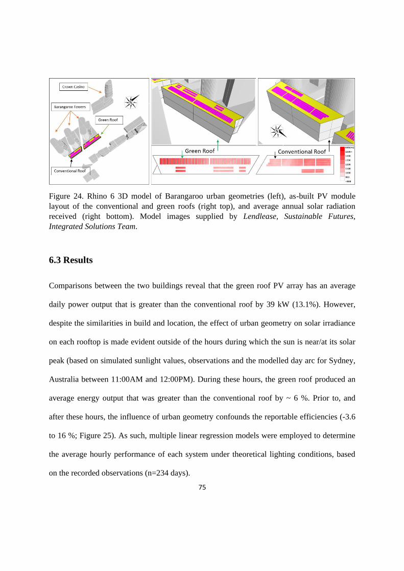
75

Figure 24. Rhino 6 3D model of Barangaroo urban geometries (left), as-built PV module

layout of the conventional and green roofs (right top), and average annual solar radiation

received (right bottom). Model images supplied by Lendlease, Sustainable Futures,

Integrated Solutions Team.

6.3 Results

Comparisons between the two buildings reveal that the green roof PV array has an average

daily power output that is greater than the conventional roof by 39 kW (13.1%). However,

despite the similarities in build and location, the effect of urban geometry on solar irradiance

on each rooftop is made evident outside of the hours during which the sun is near/at its solar

peak (based on simulated sunlight values, observations and the modelled day arc for Sydney,

Australia between 11:00AM and 12:00PM). During these hours, the green roof produced an

average energy output that was greater than the conventional roof by ~ 6 %. Prior to, and

after these hours, the influence of urban geometry confounds the reportable efficiencies (-3.6

to 16 %; Figure 25). As such, multiple linear regression models were employed to determine

the average hourly performance of each system under theoretical lighting conditions, based

on the recorded observations (n=234 days).

76

Figure 25. Average hourly energy output (kW) for each roof across all observations. Error

bars represent Standard error of the mean (SEM). Arrows [A], [B] and [C] highlight

differences in day arc shading due to urban geometries across the monitoring period (Spring,

Summer and Autumn).

The analysis was conducted for each season during which observations were recorded,

revealing that the green roof produced an increased average hourly energy output of ~ 2.48 %

at any given light level, corresponding to an average production increase of 11.3 kW per day,

or 3.63 %. It is important to note this value corresponds to overall performance increase,

under any light condition observed over the monitoring period (n=234), and that specific

performance increases would vary with environmental conditions such as weather, cloud

cover, temperature and solar pathing.

0

10

20

30

40

50

60

Energ

y P

roduction (

kW

)

Green Roof Conventional Roof

A

B

C

77

While the identification of increased production in energy is informative, the effect of these

yields is not evident to a general audience. Therefore, solar yields are often discussed in

terms of financial (money saved/earned) or social/environmental terms (CO2

mitigated/equivalent number of trees planted). Anecdotally, the consumer benefits of solar

power are primarily focused on financial gains. During the monitoring period, the green and

conventional roofs produced a total of 69 (corrected) and 59.5 MWh of clean electricity. This

equates to a monthly revenue of $2,360 and $2,036 respectively (based on retail energy prices

of $270/MWh). This means that over the 8-month monitoring period, a green roof with the

same operational parameters as the conventional roof would generate an additional $2,595 in

revenue.

Additionally, through the production of clean renewable energy, the green and conventional

roofs were able to mitigate the production of greenhouse gasses by 55.9 and 48.2 t-CO2e

(tonnes of CO2 equivalent gasses), respectively (Department of the Environment and Energy,

2020). This equates to ~ 807 and 696 trees planted, with a difference of 7.7 t-CO2e, or 110

trees planted by the green roof (Greenhouse Gas Equivalencies Calculator, 2021).

Additionally, conservative estimates from the literature (George, 2012; Heusinger and

Weber, 2017; Kuronuma et al., 2018; Shafique, Xue and Luo, 2020) indicate that the

vegetation on the green roof may have mitigated up to an additional 1.1 t-CO2 during the

monitoring period, through photosynthesis.

78

6.4 System Considerations for Comparisons

Despite the extensive corrections made to the energy outputs from the two buildings,

comparisons between PV systems are complex, and several factors must be considered. Table

15 lists the potential confounding variables identified between the systems.

Table 15. Considerations for system comparisons for solar outputs. Considerations that have

been denoted as “Y” as being considered have been incorporated into the experimental

analysis. Considerations denoted as “N” were unable to be incorporated into the analysis.

Considerations Considered Comments

System Capacity Y The peak nominal power of each roof is different, with a variance in

system size by 21.61 kWp (16.33 %).

Convection below panel N

Module azimuth (Green roof: North ballast layout; Conventional roof:

East-West accordion layout) results in different convective heat

transfer opportunities on the rear surface of the panels. Module

temperatures will be impacted by this.

Convection above panel N

Module tilt (Green roof: 15° and 2°; Conventional roof: 5°) results in

different convective heat transfer opportunities on the front surface of

the panels. Module temperatures will be impacted by this.

Insolation – array

layout Y/N

Module azimuth of each roof results in different insolation that PV

modules are exposed to.

Insolation – shading Y Modules across and between roofs will experience shading differently

due to urban geometries.

Insolation – soiling Y Modules are impacted by soiling different due to tilt, age and cleaning

routines.

Module – degradation

losses Y

System age differs between roofs and the calculated efficiency of each

system varies between manufacturers.

Module – temperature

coefficients of modules N Modules will respond to temperature fluctuations differently.

Mismatch Losses N No two modules will be electrically identical which incurs mismatch

losses. These will limit the PV performance.

6.5 Findings

Due to differences in PV panel efficiencies, system size and panel age, numerous corrections

were applied to assess the output of the green roof to be as close to representative of the

79

conventional roof performance as possible. The effect of surrounding urban geometries had a

clear influence on the amount of light available for each rooftop, so conclusions have been

drawn between the two buildings under modelled lighting conditions. Comparisons between

the two systems clearly demonstrate a substantial improvement in energy yield from the

green roof, as well as revenue generated, and CO2 emissions mitigated.

Thus theoretical retrofitting of the conventional roof in this study with an extensive green

roof with similar parameters to the studied green roof would improve the total energy

generation by up to 3.63%. This represents an increase in energy output by 2,724.4 kW, for

an equivalent time period, equating to an improved CO2 mitigation potential of up to 3.3 t-

CO2e, and an additional $729 in revenue.

It is important to note that the current analysis cannot be extended to model the full year

performance of the systems, as the observed seasonal variation in system performance is

substantial, and the effect of seasonal variation is predicted to be greater for the Winter

months. Therefore, the results expressed here should not be extrapolated to yearly, or lifetime

performance. Additionally, the effect of temperature on the performance of the panels could

not be determined due to faulty sensors over the course of the experiment. As such, the

findings presented here are generalised to the performance of the two roofs, if they were of

equal size, age and location. The nature of the cooling effect of the roof to increase solar

generation cannot be exactly determined, however it can be concluded that it was the

presence of the green roof that resulted in the specific design and layout of the green roof.

80

7 Conclusions and future directions

The current study represents one of the most objective attempts to critically and

quantitatively compare the ecosystem service performance effects of a green roof to a

building with a conventional roof. This research also provides important input into the City of

Sydney’s Green Sydney Strategy and offer additional evidence to encourage the adoption of

green roofs and support the ambitious greening targets set by the City.

Despite some differences between the matched buildings, it is nonetheless apparent that

measurable benefits can be directly attributed to the presence of the green roof related to

biodiversity provision, stormwater management, thermal insulation and PV energy

production. Whilst these effects are clear, there is nonetheless a need for continued research

in this field, notably with the growing need to quantify the benefits of green initiatives on a

financial scale. Thus, the future research following on from the current work should include:

• A return-on-investment analysis of green roof / Biosolar array implementation, both

on an individual building and city scale. This work is essential to critically credential

the potential value that can be attached to choosing green options in the future built

environment field.

• Urban biodiversity and the support green roofs and green networks (stepping-stones)

offer for species movement through the urban landscape.

81

• Assessing other benefits of green roofs. For example, it is well recognised that green

infrastructure provides value that was not assessed by the current work, notably in

terms of human health outcomes.

• Integrated modelling that incorporates the effects of green roofs and Biosolar systems

on a whole of city scale. Whilst the biodiversity, stormwater and PV energy benefits

of the tested system are clear from our work, it is well known that green infrastructure

will need to be implemented on a very large scale to gain the value necessary to build

sustainable future cities. Generalising the combined findings of many smaller studies

such as ours using computer models will be necessary to provide the projected effects

of mass scale green systems on city performance. As some benefits provided by

passive green infrastructure are of a quantitatively small magnitude relative to the

scale of the environment (specifically, air pollution abatement), large scale models are

also necessary to provide the evidence that green systems can provide real value in

these scenarios.

82

8. References

Abu-Hamdeh, N. H., Khdair, A. I. and Reeder, R. C. (2001) “Comparison of two methods used to evaluate thermal

conductivity for some soils,” International Journal of Heat and Mass Transfer, 44(5), pp. 1073–1078. doi:

10.1016/S0017-9310(00)00144-7.

Alshayeb, M. J. and Chang, J. D. (2018) ‘Variations of PV panel performance installed over a vegetated roof and a

conventional black roof’, Energies, 11(5). doi: 10.3390/en11051110.

Bai, Y., Zhao, N., Zhang, R. & Zeng, X. 2019. Storm water management of low impact development in urban areas

based on swmm. Water, 11, 33.

Ball, J. Uncertainty of gauged data and its impact on the prediction of design flood flows. 20th Congress of the Asia

Pacific Division of the International Association for Hydro Environment Engineering & Research (IAHR APD 2016),

2016.

Ball, JE, (2018), Urban drainage modelling, Keynote Address Proceedings 21st IAHR-APD Congress, IAHR,

Yogyakarta, Indonesia.

Baumann, N. 2006. Ground-nesting birds on green roofs in switzerland: preliminary observations. Urban Habitats,

4, 37-50.

Baumann, T. et al. (2019) ‘Photovoltaic systems with vertically mounted bifacial PV modules in combination with

green roofs’, Solar Energy. Elsevier, 190(August), pp. 139–146. doi: 10.1016/j.solener.2019.08.014.

Berthon, K. 2015. Invertebrates on green roofs in Sydney.

Bianco, L. et al. (2017) “Thermal behaviour assessment of a novel vertical greenery module system: first results of a

long-term monitoring campaign in an outdoor test cell,” Energy Efficiency, 10(3). doi: 10.1007/s12053-016-9473-4.

Brady, PDM and Ball, JE, (2015), Parallel and distributed SWMM for individual computation in a genetic

algorithm, Proc. 36th IAHR World Congress, The Hague, The Netherlands.

Brenneisen, S. 2006. Space for urban wildlife: designing green roofs as habitats in switzerland. Urban Habitats, 4.

Broekhuizen, I., Leonhardt, G., Marsalek, J. & Viklander, M. 2020. Event selection and two-stage approach for

calibrating models of green urban drainage systems. Hydrology and Earth System Sciences, 24, 869-885.

Chapman, C., & Horner, R. R. 2010. Performance assessment of a street-drainage biotention system. Water

Environment Research, 82. 109.

Chemisana, D. and Lamnatou, C. (2014) ‘Photovoltaic-green roofs: An experimental evaluation of system

performance’, Applied Energy. Elsevier Ltd, 119, pp. 246–256. doi: 10.1016/j.apenergy.2013.12.027.

Clean Energy Australia (2021) Clean Energy Australia 2021 Fact Sheet.

Coffman, R. R. & Davis, G. Insect and avian fauna presence on the ford assembly plant ecoroof. Third Annual

Greening Rooftops for Sustainable Communities Conference, Awards and Trade Show, 2005. 4-6.

Conn, R., Werdin, J., Rayner, J. P. & Farrell, C. 2020. Green roof substrate physical properties differ between

standard laboratory tests due to differences in compaction. Journal of Environmental Management, 261, 110206.

Currie, B. A. & Bass, B. 2008. Estimates of air pollution mitigation with green plants and green roofs using the

ufore model. Urban Ecosystems, 11, 409-422.

Czemiel-Berndtsson, J. 2010. Green roof performance towards management of runoff water quantity and quality: a

review. Ecological Engineering, 36, 351-360.

Davies, B. E., Elwood, P. C., Gallacher, J., & Ginnever, R. C. (1985). The relationships between heavy metals in

garden soils and house dusts in an old lead mining area of North Wales, Great Britain. Environmental Pollution. Series

B: Chemical and Physical, 9(4), 255–266. https://doi. org/10.1016/0143-148X(85)90002-3.

Davis, A. P. 2007. Field performance of bioretention: Water quality. Environmental Engineering Science, 24. 8.

Davis, A. P., Shokouhian, M., Sharma, H., & Minami, C. (2001). Laboratory study of biological retention for urban

stormwater management. Water Environment Research, 73(1), 5–14.

83

Davis, A. P., Shokouhian, M., Sharma, H., Minami, C., & Winogradoff, D. (2003). Water quality improvement

through bioretention: lead, copper, and zinc removal. Water Environment Research, 75, 73–82.

Department of the Environment and Energy (2020) National Greenhouse Accounts Factors October 2020. Available

at: https://www.industry.gov.au/data-and-publications/national-greenhouse-accounts-factors-2020.

Deutsch, B., Whitlow, H., Sullivan, M. & Savineau, S. 2005. Re-greening Washington DC: a green roof vision

based on environmental benefits for air quality and stormwater management.

Dromgold, J. R., Threlfall, C. G., Norton, B. A. & Williams, N. S. 2020. Green roof and ground-level invertebrate

communities are similar and are driven by building height and landscape context. Journal of Urban Ecology, 6, juz024.

Fitchett, A., Govender, P. and Vallabh, P. (2020) “An exploration of green roofs for indoor and exterior temperature

regulation in the South African interior,” Environment, Development and Sustainability, 22(6). doi: 10.1007/s10668-

019-00413-5.

Fleck, R. Gill, L. R. Pettit, T. Irga, P. J. Williams, N. L. R. Seymour, J. R. Torpy, F. R. 2020a. Characterisation of

fungal and bacterial dynamics in an active green wall used for indoor air pollutant removal. Building and Envrionemnt.

179. Doi: 10.1016/j.buildenv.2020.106987

Fleck, R. Pettit, T. J. Douglas, A. N. J. Irga, P. J. Torpy, F. R. 2020b. Bio-Based Materials and Biotechnologies for

Eco-Efficient Construction. Chapter 15: Botanical Biofiltration for reducing indoor air pollution. pp. 305-327. Doi:

10.1016/B978-0-12-819481-2.00015-5.

George, A. M. (2012) ‘The Potential Carbon Offset Represented by a Green Roof’.

Georgopoulos. (2011). Journal of Toxicology and Environmental Health, Part B: Critical Reviews Environmental

Copper: its Dynamics and Human, (2013), 37–41. doi: https://doi.org/10.1080/109374001753146207.

Glass, C., & Bissouma, S. (2005). Evaluation of a parking lot bioretention cell for removal of stormwater pollutants.

Ecosystems and Sustainable Development V (81, pp. 699–708). Southampton: WIT Press.

Grant, G. 2006. Extensive green roofs in london. Urban Habitats, 4, 51-65.

Greenhouse Gas Equivalencies Calculator (2021) United States Environmental Protection Agency.

Gregoire, B. G. & Clausen, J. C. 2011. Effect of a modular extensive green roof on stormwater runoff and water

quality. Ecological Engineering, 37, 963-969.

Hanfi, M. Y., Mostafa, M. Y. A., Zhukovsky, M. V., 2020. Heavy metal contamination in urban surface sediments:

sources, distribution, contamination control and remediation. Environmental Monitoring and Assessment. 192. 1. DOI:

10.1007/s10661-019-7947-5

Heusinger, J. and Weber, S. (2017) ‘Extensive green roof CO2 exchange and its seasonal variation quantified by

eddy covariance measurements’, Science of the Total Environment. Elsevier B.V., 607–608, pp. 623–632.

Hicks, B, Gray, S and Ball, JE, (2009), A Critical Review of the Urban Rational Method, Proc of H2009, 32nd

Hydrology and Water Resources Symposium, Engineers Australia, Newcastle, Australia, ISBN 978-08258259461.

Hicks, B., Gray, S. & Ball, J. A critical review of the urban rational method. h2009: 32nd hydrology and water

resources symposium, newcastle: adapting to change, 2009. Engineers Australia, 1424.

Hsieh, C., & Davis, A. P. (2005). Evaluation and optimization of bioretention media for treatment of urban storm

water runoff. Journal of Environmental Engineering, 131(11), 1521–1531.

Hui, S. C. M. and Chan, S. C. (2011) ‘Integration of green roof and solar photovoltaic systems’, in Joint Symposium

2011: Integrated Building Design in the New Era of Sustainability, pp. 1–12.

Hunt, W. F., Jarrett, A. R., Smith, J. T., & Sharkey, L. J. (2006). Evaluating bioretention hydrology and nutrient

removal at three field sites in North Carolina. Journal of Irrigation and Drainage Engineering, 132(6), 600–608.

Hunt, W. F., Smith, J. T., Jadlocki, S. J., Hathaway, J. M., & Eubanks, P. R. 2008. Pollutant removal and peak flow

mitigation by a bioretention cell in urban Charlotte, NC. Journal of Environmental Engineering, 5. 134.

Jahanfar, A. et al. (2020) ‘An experimental and modeling study of evapotranspiration from integrated green roof

photovoltaic systems’, Ecological Engineering. Elsevier, 152(July 2019), p. 105767. doi:

10.1016/j.ecoleng.2020.105767.

Jayasooriya, V., NG, A., Muthukumaran, S. & Perera, B. 2017. green infrastructure practices for improvement of

84

urban air quality. Urban Forestry & Urban Greening, 21, 34-47.

Jiries, A. G., Hussein, H. H., & Halaseh, Z. (2001). The quality of water and sediments of street runoff in Amman.

Jordan, 824, 815–824. https://doi.org/10.1002/hyp.186.

Kalantari, Z., Ferreira, C. S. S., Keesstra, S. & Destouni, G. 2018. Nature-based solutions for flood-drought risk

mitigation in vulnerable urbanizing parts of East-Africa. Current Opinion in Environmental Science & Health, 5, 73-78.

Köhler, M. 2006. Long-term vegetation research on two extensive green roofs in berlin. Urban Habitats, 4, 3-26.

Kuczera, G., Kavetski, D., Franks, S. & Thyer, M. 2006. Towards a bayesian total error analysis of conceptual

rainfall-runoff models: characterising model error using storm-dependent parameters. Journal of Hydrology, 331, 161-

177.

Kumar, P., Druckman, A., Gallagher, J., Gatersleben, B., Allison, S., Eisenman, T. S., Hoang, U., Hama, S., Tiwari,

A., Sharma, A., Abhijith, K. V., Adlakha, D., Mcnabola, A., Astell-Burt, T., Feng, X., Skeldon, A. C., de Lusignan, S.

& Morawska, L. 2019. The nexus between air pollution, green infrastructure and human health. Environment

International, 133, 105181.

Kuronuma, T. et al. (2018) ‘CO2 Payoffof extensive green roofs with different vegetation species’, Sustainability

(Switzerland), 10(7), pp. 1–12. doi: 10.3390/su10072256.

Libessart, L. and Kenai, M. A. (2018) “Measuring thermal conductivity of green-walls components in controlled

conditions,” Journal of Building Engineering, 19.

Lin. BS., Yu. CC., Su. AT., Lin. YJ. 2013. Impact of climate conditions on the thermal effectiveness of an extensive

green roof. Building and Environment, 67, 26-33.

Lundholm, J. T. (2015) “Green roof plant species diversity improves ecosystem multifunctionality,” Journal of

Applied Ecology, 52(3). doi: 10.1111/1365-2664.12425. Hoffmann, S. and Koehl, M. (2014) “Effect of humidity and

temperature on the potential-induced degradation,” Progress in Photovoltaics: Research and Applications, 22(2), pp.

173–179.

MacIvor, M. S. & Lundholm, J. 2011. Insect species composition and diversity on intensive green roofs and

adjacent level-ground habitats. Urban Ecosystems, 14, 225-241.

Mentens, J., Raes, D. & Hermy, M. 2006. Green roofs as a tool for solving the rainwater runoff problem in the

urbanized 21st century? Landscape and Urban Planning, 77, 217-226.

Morau, D., Libelle, T. and Garde, F. (2012) “Performance evaluation of green roof for thermal protection of

buildings in reunion Island,” in Energy Procedia. Elsevier, pp. 1008–1016. doi: 10.1016/j.egypro.2011.12.1047.

Nowak, D. J., Crane, D. E. & Stevens, J. C. 2006. Air pollution removal by urban trees and shrubs in the united

states. Urban Forestry & Urban Greening, 4, 115-123.

Ogaili, H. and Sailor, D. J. (2016) ‘Measuring the Effect of Vegetated Roofs on the Performance of Photovoltaic

Panels in a Combined System’, Journal of Solar Energy Engineering, Transactions of the ASME, 138(6), pp. 1–8. doi:

10.1115/1.4034743.

Oksanen, J., Guillaume, B. F., Friendly. M., Kindt. R., Legendre. P., McGlinn. D., Minchin. P. R., O’Hara. R. B.,

Simpson. G. L., Solymos. P., Stevens. H. M., Szoecs. E., Wagner. H., 2020. Community Ecology Package (Vegan).

URL: https://cran.r-project.org; https://github.com/vegandevs/vegan.

Osma, G. et al. (2016) ‘The impact of height installation on the performance of PV panels integrated into a green

roof in tropical conditions’, in Energy Production and Management in the 21st Century II: The Quest for Sustainable

Energy, pp. 147–156. doi: 10.2495/eq160141.

Ottele, M. and Perini, K. (2017) “Comparative experimental approach to investigate the thermal behaviour of

vertical greened facades of buildings,” Ecological Engineering, 108, pp. 152–161. doi: 10.1016/j.ecoleng.2017.08.016.

Pearce, H. & Walters, C. L. 2012. Do green roofs provide habitat for bats in urban areas? Acta Chiropterologica, 14,

469-478.

Peng, Z. & Stovin, V. 2017. Independent validation of the swmm green roof module. Journal of Hydrologic

Engineering, 22, 04017037.

Perez, M. J. R. et al. (2012) ‘Green-roof integrated pv canopies-an empirical study and teaching tool for low income

85

students in the South Bronx’, in World Renewable Energy Forum, WREF 2012, Including World Renewable Energy

Congress XII and Colorado Renewable Energy Society (CRES) Annual Conferen, pp. 4046–4052.

Perini, K. et al. (2011) “Vertical greening systems and the effect on air flow and temperature on the building

envelope,” Building and Environment, 46(11). doi: 10.1016/j.buildenv.2011.05.009.

Pétremand, G., Chittaro, Y., Braaker, S., Brenneisen, S., Gerner, M., Obrist, M. K., Rochefort, S., Szallies, A. &

Moretti, M. 2018. Ground beetle (Coleoptera carabidae) communities on green roofs in switzerland: synthesis and

perspectives. Urban Ecosystems, 21, 119-132.

Polo-Labarrios, M. A. et al. (2020) “Comparison of thermal performance between green roofs and conventional

roofs,” Case Studies in Thermal Engineering, 21, p. 100697. 0.1016/j.csite.2020.100697.

Pourkhabbax, A. Rastin, N. Olbrich, A. Langenfeld-Heyser, R. Polle, A. 2010. Influence of environmental pollution

on leaf properties of urban plane trees, Platanus orientalis L. Bulletin for Environmental Contamination and Toxicology.

85 (3): pp. 251-255. Doi: 10.1007/s00128-010-0047-4.

R Core Team, 2020. R: A language for statistical computing. R Foundation for Statistical Computing, Vienna,

Austria. URL: https://www.R-Project.org/.

Rasmussen. K.H., Taheri. M., & Kabel. R. L., 1975. Global emissions and natural processes for removal of gaseous

pollutants. Water Air Soil Pollution, 4, 33-64. 10.1007/BF01794130

Reddy, K. R., Zie, T. Dastgheibi, S. 2012. Removal of heavy metals from urban stormwater runoff using different

filter materials. Journal of Environmental Chemical Engineering. 2. 1. DOI: 10.1016/j.jece.2013.12.020.

Renard, B., Kavetski, D., Kuczera, G., Thyer, M. & Franks, S. W. 2010. Understanding predictive uncertainty in

hydrologic modeling: the challenge of identifying input and structural errors. Water Resources Research, 46.

Roseen, R. M., Ballestero, T. P., Houle, J. J., Avelleneda, P., Wildey, R., & Briggs, J. (2006). Stormwater low-

impact development, conventional structural, and manufactured treatment strategies for parking lot runoff.

Transportation Research Record: Journal of the Transportation Research Board, Washington, D.C.: Transportation

Research Board of the National Academies, 1984, 135–147.

Rosenfeld, A. H., Akbari, H., Romm, J. J. & Pomerantz, M. 1998. Cool communities: strategies for heat island

mitigation and smog reduction. energy and buildings, 28, 51-62.

Rossman, L. A. 2010. Storm Water Management Model Eser's Manual, Version 5.0, National Risk Management

Research Laboratory.

Rossman, LA, (2015), Storm Water Management Model User’s Manual Version 5.1, U.S. Environmental Protection

Agency, Cincinnati, OH, USA

Rowe, D. B. 2011. Green roofs as a means of pollution abatement. Environmental Pollution, 159, 2100-2110.

Shafique, M., Luo, X. and Zuo, J. (2020) “Photovoltaic-green roofs: A review of benefits, limitations, and trends,”

Solar Energy, 202, pp. 485–497. doi: 10.1016/j.solener.2020.02.101.

Shafique, M., Xue, X. and Luo, X. (2020) ‘An overview of carbon sequestration of green roofs in urban areas’,

Urban Forestry and Urban Greening. Elsevier, 47(October 2019), p. 126515. doi: 10.1016/j.ufug.2019.126515.

She, N. & Pang, J. 2010. Physically based green roof model. Journal of Hydrologic Engineering, 15, 458-464.

Soulis, K. X., Valiantzas, J. D., Ntoulas, N., Kargas, G. & Nektarios, P. A. 2017. Simulation of green roof runoff

under different substrate depths and vegetation covers by coupling a simple conceptual and a physically based

hydrological model. Journal of Environmental Management, 200, 434-445.

Speak, A. 2013. Quantification of the Environmental Impacts of Urban Green Roofs, the University of Manchester

(United Kingdom).

Stovin, V. R., Moore, S. L., Wall, M. & Ashley, R. M. 2013. The potential to retrofit sustainable drainage systems

to address combined sewer overflow discharges in the thames tideway catchment. Water and Environment Journal, 27,

216-228.

Sun, N., Hall, M., Hong, B. & Zhang, L. 2014. Impact of SWMM catchment discretization: case study in Syracuse,

New York. Journal of Hydrologic Engineering, 19, 223-234.

Sun, T., Bou-Zeid, E., Wang, Z.-H., Zerba, E. & Ni, G.-H. 2013. Hydrometeorological determinants of green roof

86

performance via a vertically-resolved model for heat and water transport. Building and Environment, 60, 211-224.

Sun, X. L., & Davis, A. P. (2007). Heavy metal fates in laboratory bioretention systems. Chemosphere, 66(9), 1601–

1609.

Sydney Water, 2015. Stormwater, Our role in managing floods. Document SW 78 09/15. Available at:

sydneywater.com.au

Tan, P. Y. & Sia, A. A pilot green roof research project in Singapore. Proceedings of Third Annual Greening

Rooftops for Sustainable Communities Conference, Awards and Trade Show, Washington, DC, 2005.

Umakhanthan, K and Ball, JE, (2005), Rainfall Models for Catchment Simulation, Australian Journal of Water

Resources, 9(1):55-67.

Villarreal, E. L. & Bengtsson, L. 2005. Response of a sedum green-roof to individual rain events. Ecological

Engineering, 25, 1-7.

Wang, J. W., Poh, C. H., Tan, C. Y. T., Lee, V. N., Jain, A. & Webb, E. L. 2017. Building biodiversity: drivers of

bird and butterfly diversity on tropical urban roof gardens. Ecosphere, 8, e01905.

Wilkinson, S. and Dixon, T. (2016) Green Roof Retrofit: Building Urban Resilience. 1st edn. United Kingdom: John

Wiley & Sons, Ltd.

Williams, N. S. G., Lundholm, J. & Scott-Macivor, J. 2014. Forum: Do green roofs help urban biodiversity

conservation? Journal of Applied Ecology, 51, 1643-1649.

Wong, N. H., Tan. P. Y., & Chen. Y. 2007. Study of thermal performance of extensive rooftop greenergy systems in

the tropical climate. Building and Environment, 42, 25-54.

Yang, J. & Wang, Z.-H. 2014. Physical parameterization and sensitivity of urban hydrological models: application

to green roof systems. uilding and Environment, 75, 250-263.

Yang, J., Yu, Q. & Gong, P. 2008. Quantifying air pollution removal by green roofs in chicago. Atmospheric

Environment, 42, 7266-7273.

Zaghoul, NA, (1983), Sensitivity Analysis of the SWMM Runoff-Transport Parameters and the Effects of

Catchment Discretisation, Advances in Water Resources, 6:214

Zannetti, P. 1990. Dry and wet deposition. Air pollution modelling. Springer, Boston, MA. 10.1007/978-1-4757-

4465-1_10

Zhang, R., Chen, G., Yin, Z., Zhang, Y. & Ma, K. 2021. Urban greening based on the supply and demand of

atmospheric PM2.5 removal. Ecological Indicators, 126, 107696.

Zhang, Z., Szota, C., Fletcher, T. D., Williams, N. S. G., Werdin, J. & Farrell, C. 2018. Influence of plant

composition and water use strategies on green roof stormwater retention. Science of the Total Environment, 625, 775-

781.

Zhao, Q., Myint. S. W., Wentz. E., Fan. C., 2015. Rooftop surface temperature analysis in an urban residential

environment. Remote Sensing, 7, 12135-12159.

Zheng, X., Zou, Y., Lounsbury, A. W., Wang, C. & Wang, R. 2021. Green roofs for stormwater runoff retention: A

global quantitative synthesis of the performance. Resources, Conservation and Recycling, 170, 105577.