Jump and Cojump Risk in Subprime Home Equity Derivatives · Jump and Cojump Risk in Subprime Home Equity Derivatives Bruce ... mergers of Bear Stearns with JP ... power as long as

Jump and Cojump Risk in Subprime Home Equity Derivatives

Bruce Mizrach�

Rutgers University

Revised: July 2009

Abstract

I analyze the jump risk in the ABX index of subprime home equity credit default swaps andCME housing futures. Using estimators of the jump and cojump components of security prices, Idocument: (1) signi�cant jumps in the ABX as early as September 2006, well before any problemsin the mortgage market were discussed in the press or policy circles; (2) news explains up to 56%of the jump risk; (3) the return variation due to jumps in the housing futures is above 40%, almosttwo times larger than the ABX; (4) 27 signi�cant cojump episodes between the ABX and housingfutures; (5) a predictive model that explains up to 85% of the jump risk; (6) a 20 point slope in thehousing futures curve leads to an expected jump of �1:4% in the BBB- ABX; (7) jumps explainup to 50% of the value-at-risk exceedences which occur at almost three times the expected rate.

Keywords: asset backed securities; credit default swaps; housing futures; subprime; jump risk;cojumps; Value-at-Risk;

JEL Classification: G13, G32, E44;

� Department of Economics, Rutgers University, e-mail: [email protected], (732) 932-7363 (voice)and (732) 932-7416 (fax). http://snde.rutgers.edu. I would like to thank MarkIt for providing the ABXdata. Jens Hilscher, Paul Kupiec, Chris Neely, Clara Vega, Hao Zhou and seminar participants at NCTU,Hong Kong Monetary Authority, East Carolina, Brandeis, Villanova, HEC, Norges Bank, Bank of CanadaFixed Income Conference, World Bank/IMF Conference on Risk Management, and the INQUIRE EuropeConference on Liquidity provided useful comments.

1. Introduction

Asset backed securities in residential real estate diversify credit risk and indirectly bene�t home

owners through lower �nancing rates. This market includes both residential mortgage backed

securities (RMBS) and home equity loans (HEL). The HEL segment, which includes both �rst and

second lien mortgages,1 has grown to nearly $600 billion by the end of 2007 and helped to raise

U.S. home ownership rates to a 2005 peak of 69%.

In the spring of 2007, these instruments came into focus with a collapse in credit markets

around the world. Particular attention was paid to the so-called subprime market, a subset of

home borrowers who failed to meet conventional mortgage qualifying criteria. These borrowers

constitute an important class of the residential real estate market, particularly in recent years. The

Harvard Joint Center for Housing Studies (2008) estimates that the subprime share of mortgage

originations exceeded 20% in 2006, up from less than 7% in 2002.

As real estate prices began to fall, in some areas as early as 2005, these subprime borrowers

began to have trouble making their payments. The Mortgage Bankers Association (MBA) survey

for the �rst quarter of 2009 showed a delinquency rate of 8:22%, up from 1:6% in the �rst quarter

of 2006. 3:85% of all loans and 14:34% of subprime loans are in foreclosure, the highest levels

recorded in the MBA survey since its 1979 inception.

Housing sector �nancial intermediaries have su¤ered major losses. New Century, a California

based lender specializing in the subprime market, declared bankruptcy on April 1, 2007. Coun-

trywide, the largest servicer of subprime mortgages, experienced a decline in shareholder equity

of �78:7% in 2007 before being acquired by Bank of America in January 2008. Washington Mu-

tual, the nation�s largest thrift, was seized by the FDIC on September 25, 2008. There were 26

bank failures in 2008, resulting in $22:3 billion in cash outlays from the Deposit Insurance Fund,

and there have been an additional 52 failures in 2009. The forced mergers of Bear Stearns with

JP Morgan (March 2008), Merrill Lynch with Bank of America, and the bankruptcy of Lehman

Brothers (both in September 2008) have permanently changed the investment banking landscape.

The Treasury and the Federal Reserve have assumed more than $7:5 trillion in direct and indirect

�nancial obligations to try to stabilize the �nancial system.

This paper attempts to assess market risks associated with the ongoing subprime �nancial

1 First-lien sub-prime mortgage loans as well as second-lien home equity loans and home equity lines of creditare all part of what is called the home equity asset backed security sector. Ashcraft and Scheurmann (2008)note that other non-conventional mortgages, including Alt-A and Jumbo loans, are classi�ed as RMBS.

2

crisis. I analyze two derivative securities markets that are closely linked to changes in home prices

and a¤ordability. The �rst of these is the ABX.HE index, compiled by MarkIt, an independent

provider of credit derivatives pricing. The ABX aggregates prices of credit default swaps on

subprime mortgage backed securities.

The ABX index has been used to provide long and short exposure during the credit crisis and

to price illiquid mortgage backed securities. Goldman Sachs�structured products trading group

earned more than $4 billion in pro�ts in 2007 by buying default protection through the ABX.2

John Paulson�s Credit Opportunities hedge fund returned 589:9% in 2007 speculating on a decline

in subprime mortgages using the ABX, generating pro�ts of $15 billion and Paulson a personal

gain of $3:7 billion.

Motivated by the new accounting rule FAS 157, banks have been prompted to mark their

securities to market prices rather than models.3 The ABX is being used for valuation of a wide range

of illiquid mortgage securities.4 Estimated mark-to-market losses at U.S. �nancial institutions have

now reached $2:7 trillion.5

The second instrument which the paper analyzes is the Chicago Mercantile Exchange�s resi-

dential real estate market futures. These contracts began trading in the Spring of 2006 and have

provided a way to hedge the value of individual homes. The futures contracts track a repeat sales

housing index originally constructed by Case and Shiller (1989).

Contracts trade at a variety of maturities, ranging from one month to several years. The term

structure of prices is currently �attened, indicating that the market anticipates housing prices may

have stabilized. In mid-July 2009, the composite index price for August 2009 was at 147:40; less

than 2% above the 145:00 closing price for the August 2010 settlement.

I rely on the recent methods introduced by Barndor¤-Nielsen and Shephard (2006) to extract

the jump risk component from these derivative security prices. The procedure isolates the portion

of security returns coming from discontinuous movements or jumps in the underlying stochastic

process. I use Huang and Tauchen�s (2005) estimator of relative jumps to assess statistical signi�-

cance. In Mizrach (2009), I show that these methods, even at a daily frequency, can be useful in

2 TheWall Street Journal December 14, 2007. The article notes that Goldman traded primarily in the BBB-tranche of the ABX index for the second half of 2006.3 The Financial Accounting Standards Board (FASB) passed rule 157, Fair Value Measurements, in Septem-ber of 2006, and the rule went into e¤ect on November 15, 2007.4 Fender and Scheicher (2008) acknowledge this industry practice, but caution that, because of the limitedset of securities in the index, the ABX may not be a good predictor of future cash �ows in this market.5 International Monetary Fund, Global Financial Stability Report, April 2009.

3

analyzing sudden market movements. This paper assesses their small sample properties using a

Monte Carlo exercise and �nds good power as long as the jump contribution to total variance is

not too small.

I detect signi�cant jump risk across all the credit quality tranches of the ABX as early as

September 2006, long before the ABX index had shown any signs of weakness and was trading

above par. The jump episodes correspond closely to economic news which I have collected from

public and private sector reports on the subprime crisis. News dummies explain up to 56% of the

variation in the jump risk.

Jumps in the housing futures explain more than 40% of the total return variation, and the 1-

and 12-month contracts both experience signi�cant jumps on nearly 2 out 3 days in the sample.

These jumps are not, overall, related to news about the ABX, but I still �nd an important linkage

between the levels and jumps of the housing futures and the subprime index.

I isolate common movements across the two markets using a measure of cojump risk introduced

by Bollerslev, Law and Tauchen (2008). Beine, Lahaye, Laurent, Neely and Palm (2007) examine

cojump risk in foreign exchange due to central bank intervention and Lahaye, Laurent and Neely

(2007) analyze the e¤ect of macroeconomic announcements on cojumps across stock, bond, foreign

exchange and commodity markets.

There is, at the moment, no asymptotic theory for cojump processes, so I again undertake a

Monte Carlo analysis. A studentized moving average of the daily return cross products shows good

power for detecting cojumps. I �nd 25 or more signi�cant cojumps between the futures and the

ABX. Unlike the jump risk in the futures series, news dummies explain up to 42% of the cojump

risk.

The cojump analysis is synthesized with estimates of a predictive model for ABX jump risk. I

specify current jump risk as a function of lagged jump risk, squared jump risk, the jump risk in

the housing futures and the slope of the housing futures curve. The model explains up to 85% of

the jumps. The slope of the housing futures has signi�cant explanatory power for jumps in 3 of

the 5 tranches. For the BBB- tranche, a slope of 20 points in the futures curve, a level reached

during the peak of the housing bubble, implies an expected daily jump of �1:4%:

The �nal section of the paper analyzes the importance of jumps for bank capital requirements

and risk management. Basel II (2006, p.163) requires that value-at-risk (V aR) capture �speci�c

risk ....and event risk (where the price of an individual debt or equity security moves precipitously

4

relative to the general market, e.g. on a takeover bid or some other shock event; such events would

also include the risk of �default�).� I form a hedged portfolio that is long the ABX and short the

housing futures and calculate the V aR with static and dynamic hedging. I �nd that exceedences

are nearly three times what the normal distribution would imply and that up to 50% of these large

losses can be attributed to jumps.

Section 2 begins with details about the asset backed mortgage securities market which the ABX

tracks. Section 3 develops the methodology for extracting jumps and assessing their statistical

signi�cance. Section 4 conducts Monte Carlo analysis of the daily jump estimator. Section 5

provides estimates for the jump risk across all the credit quality tranches of the ABX. Section 6

links the jump risk with the news �ow in the markets about the subprime crisis. Section 7 describes

the real estate futures market, and in Section 8, I analyze the jump risk in the CME futures prices.

In Section 9, I analyze the cojump risk between the two housing derivatives markets, and I then use

a predictive model in Section 10 to summarize their interactions. Section 11 analyzes value-at-risk

of a hedged ABX portfolio. I conclude with a limited set of policy implications and ideas for future

research in Section 12.

2. Data: ABX

2.1 Asset backed securities

Asset backed securities (ABS) are structured �xed income instruments that distribute cash �ows

from a designated pool of loans. By pooling across households and regions, they mitigate the

idiosyncratic risk of any individual borrower.

The corporate �nance motivations behind asset securitization are related to capital market

imperfections. In principal, securitizing should not e¤ect the value of the �rm. As Minton, Opler

and Stanton (1999) note, the �rm should be indi¤erent between issuing asset-backed and unsecured

debt.

Lang, Poulsen and Stulz (1995) emphasize agency costs of managerial discretion as one motive.

The �rm may �nd it more e¢ cient to create a special purpose vehicle (SPV) to monitor the cash

�ows. These SPVs are typically legally distinct entities that provide no explicit recourse to the

sponsoring �rm�s assets, eliminating the credit exposure from the �rm�s balance sheet. The net

impact of improved monitoring and credit risk insulation is that the SPV often achieves a higher

5

credit rating than the originator.

Research on ABS indicates that the market assumes there is some implicit recourse from the

sponsoring �rm and the SPV. Gorton and Souleles (2006) �nd in a sample of over 400 SPVs that

poorly rated sponsors had to promise more than 50 basis points of additional yield on average,

regardless of the credit rating of the SPV.

On balance, Thomas (2001) shows, the securitization process is wealth creating for the �rm

that sells the assets. The bene�ts may be even larger for �rms, like banks, whose capital base is

closely regulated.

The securities bundle cash �ows, transforming, as Jobst (2007) notes, an illiquid set of receiv-

ables into tradable claims or tranches. The division into distinct slices of risk and maturity makes

the securities attractive to a wide array of potential buyers.

The market has grown substantially over the last decade. In 1996, there was a total of $404

billion in asset backed securities, with credit card receivables ($181 billion) and auto loans ($71

billion) the two largest categories.

[Insert Table 1 Here]

Between 1996 and 2007, the market grew by almost 18% per year to reach a total of $2; 472

billion. I now turn to the home equity loans (HEL) securities that are the focus of this paper.

2.2 Home equity loans

In 2004, as housing prices were reaching their peak and low interest rates were making re�nancing

a popular choice for homeowners, HEL securities surpassed credit card receivables as the largest

category of asset backed securities, $454 versus $391 billion. From 1996 to 2007, they grew nearly

25% per year. In 2007 alone, the Securities Industry and Financial Markets Association (SIFMA)

reported issuance of $222 billion in HEL.6

Thomas (2001) documents that the majority of HEL loans are cash out re�nancing, with the

cash �ows used to consolidate debt, pay for education, or to make home improvements. For more

than a decade, these loans have been made available to subprime borrowers. These high risk

6 The data are from the Securities Industry and Financial Markets Assocation (SIFMA), �U.S. MarketOutlook,� January 2008. There was an additional $473 billion in non-GSE Alt-A and prime mortgagesecuritizations.

6

borrowers, according to Standard and Poor�s,7 have Fair Isaac & Co. (FICO) credit scores in the

low 600s, high loan to value (LTV) ratios, and they may lack documentation of their income or

assets.

As the credit crunch unfolded in 2007, HEL credit spreads grew due to deteriorating collateral,

and downgrades from the credit rating agencies followed. According to SIFMA, �in excess of 95

percent of ABS downgrades in the 2005-2007 vintages sector were HEL.�So while HEL securities

face systematic risk from changes in fundamentals, di¤erent tranches are particularly vulnerable.

Bloomberg estimates that a 10% default rate would wipe out the BBB rated portion of a subprime

CDO, 14% the A, and 23% for the AA.8

In 2008, new issuance e¤ectively stopped. Only $1:8 billion in home equity ABS was issued in

the �rst half of the year. By the end of the third quarter 2008, the outstanding stock of HEL ABS

fell �40:23% to $418 billion.9

2.3 Credit default swaps

One mechanism for hedging this risk was a new instrument known as a credit default swap. Credit

default swaps are derivative securities that pay security holders contingent upon a credit event.

Typically, these are triggered by some failure to deliver the underlying cash �ows promised to the

security pool. There are now very liquid markets in credit default swaps on corporate and sovereign

bonds.

Credit default swaps on ABS reference individual tranches from an SPV because they have a

wide range of default probabilities. Other unique features of asset backed securities are: (1) the

amortization of principal; (2) adjustment of security values in light of partial interest shortfalls or

principal writedown.10 Both considerations require a careful de�nition of default and settlement

procedures. The market has, since 2006, begun to standardize around the International Swaps

and Derivatives Association CDS template. To enhance transparency, the Depository Trust and

Clearing Corporation began to publish, in October 2008, the outstanding positions on a wide range

of CDS contracts, including the ABX.

With home equity securities, credit default swaps provide a sequence of payments to the pro-

7 Victoria Wagner, �Credit FAQ: Will Subprime Woes Spread To The Wider Mortgage Market?,�March 13,2007.8 Mark Gilbert �AAA Grades on Subprime CDOs May Give Cold Comfort,�Bloomberg, July 19, 2007.9 Auto loans fell almost as much, down �29:65% to $153 billion.10 The principal can also be written back up in the event of catchup payments by the security pool.

7

tection buyer. For this reason, the contracts are often referred to as pay-as-you-go. The protection

seller will compensate for losses in principal and any interest shortfall. These di¤er from corporate

credit default swaps which usually involve a single payment after a credit event. Because the ma-

turity of the ABS contract is usually the same as the underlying mortgage securities, ABS credit

default swaps can have long maturities. Corporate bond contracts typically last only �ve years.

2.4 The ABX indices

2.4.1 Entities

The ABX indices are aggregators of the performance of a variety of credit default swaps on asset

backed securities. MarkIt Ltd., a London based source of credit derivatives information, collects

information on individual credit default swaps and produces a series of indices that have become

benchmarks for the industry. This paper studies the ABX.HE indices which track home equity

loans.

MarkIt has eight criteria for including a security in the index: (a) deals from the largest 25

issuers (by sub-prime home equity issuance); (b) issued within the last six months (c) o¤ering size

of at least $500 million; (d) at least 90% �rst lien mortgages; (e) weighted average FICO credit

score less than 660; (f) Deals must pay on the 25th of the month; (g) referenced tranches must

bear interest at a �oating rate benchmark of one-month LIBOR; (h) at issuance, each deal must

have tranches of the required ratings with a weighted average life greater than four years, except

the AAA which must have an average life of longer than �ve years.

From a list of 54 reference obligations that met the MarkIt criteria, 20 distinct securities were

chosen to form the ABX HE-061 index which was constituted on January 11, 2006. The index

began trading on January 19, 2006. There have been subsequent indices formed, known as rolls,

every six months, with HE-062 pricing beginning on July 19, 2006, HE-071 on January 19, 2007,

and HE-072 on July 19, 2007. There are �ve credit tranches to each of the underlying exposures,

AAA, AA, A, BBB and BBB-. Ratings are determined by the lower of the Moody�s or Standard

& Poor�s grades.

The 15 issuers that make up the initial ABX index are in the �rst column of Table 2.


Nearly every major current and former investment bank is represented including Barclays, Bear

8

Stearns, Deutsche Bank, Goldman Sachs, JP Morgan, Lehman, Merrill Lynch, Morgan Stanley and

UBS. Non-bank �nancial intermediaries include GMAC. There are also mortgage originators like

Ameriquest, Countrywide, First Franklin, and New Century.

With the recent turmoil in the credit markets, particularly in home equity, MarkIt was unable

to constitute an index for 2008. On December 19, 2007, they released a statement that they would

postpone the launch of HE 08-1: �Under current index rules, only �ve deals quali�ed for inclusion

in the MarkIt ABX.HE 08-1. MarkIt and the dealer community considered amending the index

rules to include deals which failed to qualify initially but decided against this approach at this

time.�On May 14, 2008, MarkIt introduced the �penultimate ABX,�a new more senior slice of

the AAA tranche for the 07-2 roll. It currently trades about 10% above the AAA. As of this

writing, January 2009, there have been no new rolls of the ABX since July 2007.

The characteristics of the HE-061, HE-062 and HE-071 deals are summarized in Table 3.


While the deals have progressively lower FICO scores, and less documentation, the loan to

value ratio also falls slightly to o¤set these risks.11 The characteristics clearly indicate a very clean

exposure to high risk borrowers. While liquidity has fallen o¤ recently, the ABX indices constitute

the best available aggregate indicator of subprime borrowing and are now widely used to mark to

market institutional portfolios.

2.4.2 Cash �ows and prices

I analyze the �ve credit quality tranches of the four rolls of the ABX during the period January

19, 2006 to November 2, 2007. The data were provided to me by MarkIt.

When the ABX indexes are released, they trade at or close to par. Coupon rates for the various

releases and credit tranches are in Table 4.


When the index is selling at par, a purchaser of default protection pays only the coupon rate.

To protect $1 million in security value in the AAA tranche of the 06-1 index, for example, you will

11 Bhardwaj and Sengupta (2008) �nd, using loan level data, that there was no dramatic weakening oflending standards in the subprime market after 2004. Keys, Mukherjee, Seru and Vig (2008) caution thatsecuritization practices adversely a¤ected the screening process and made securitized subprime loans 10-25%more likely to default.

9

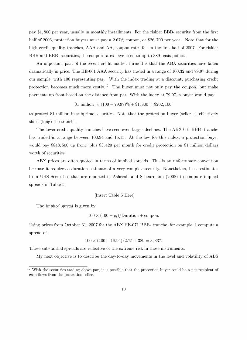
pay $1; 800 per year, usually in monthly installments. For the riskier BBB- security from the �rst

half of 2006, protection buyers must pay a 2:67% coupon, or $26; 700 per year. Note that for the

high credit quality tranches, AAA and AA, coupon rates fell in the �rst half of 2007. For riskier

BBB and BBB- securities, the coupon rates have risen to up to 389 basis points.

An important part of the recent credit market turmoil is that the ABX securities have fallen

dramatically in price. The HE-061 AAA security has traded in a range of 100:32 and 79:97 during

our sample, with 100 representing par. With the index trading at a discount, purchasing credit

protection becomes much more costly.12 The buyer must not only pay the coupon, but make

payments up front based on the distance from par. With the index at 79:97, a buyer would pay

$1 million � (100� 79:97)% + $1; 800 = $202; 100:

to protect $1 million in subprime securities. Note that the protection buyer (seller) is e¤ectively

short (long) the tranche.

The lower credit quality tranches have seen even larger declines. The ABX-061 BBB- tranche

has traded in a range between 100:94 and 15:15. At the low for this index, a protection buyer

would pay $848; 500 up front, plus $3; 420 per month for credit protection on $1 million dollars

worth of securities.

ABX prices are often quoted in terms of implied spreads. This is an unfortunate convention

because it requires a duration estimate of a very complex security. Nonetheless, I use estimates

from UBS Securities that are reported in Ashcraft and Scheurmann (2008) to compute implied

spreads in Table 5.


The implied spread is given by

100� (100� pt)=Duration+ coupon:

Using prices from October 31, 2007 for the ABX.HE-071 BBB- tranche, for example, I compute a

spread of

100� (100� 18:94)=2:75 + 389 = 3; 337:

These substantial spreads are re�ective of the extreme risk in these instruments.

My next objective is to describe the day-to-day movements in the level and volatility of ABS

12 With the securities trading above par, it is possible that the protection buyer could be a net recipient ofcash �ows from the protection seller.

10

protection, and link to the risk of correlated assets. I turn now to the modeling of discontinuous

jumps in this index.

3. Jump Processes

Consider a stochastic volatility model with jumps,

dpt = �tdt+ �tdw1;t + Jtdqt; (1)

d�2t = �(� � �2t )dt+ q�2tdw2;t; (2)

where pt is the log price of the underlying asset, �t is its drift, �t is the local volatility, w1;t and w2;t

are standard Brownian motions with correlation �, qt is a Poisson process with intensity �t, and

Jt is a normally distributed jump process with mean �J and and standard deviation �J . De�ne

the within day return process,

rt;j = pt�1+ j

M� pt�1+ j�1

M; j = 1; 2; : : :M: (3)

The quadratic variation for the daily return process is then

[r; r]t =R tt�1 �

2sds+

Pt�1<s�t J

2s : (4)

Estimation of the quadratic variation proceeds with discrete sampling from the log price process.

The realized volatility is

RVt =PMj=1 r

2t;j : (5)

In the standard stochastic volatility model, J = 0, researchers have employed realized volatility as

an estimator of the integrated volatility,R tt�1 �

2sds:

In the case of discontinuous price paths, Barndor¤-Nielsen and Shephard (2006) show that the

realized volatility will also include the jump component, and that, in the limit, realized volatility

will capture the entire quadratic variation,

limM�!1

RVt = [r; r]t (6)

To extract the integrated volatility from (6), Barndor¤-Nielsen and Shephard have also introduced

the realized bi-power variation,

BVt = ��21

PMj=1 jrt;j j jrt;j�1j (7)

11

where �1 =p2=�: It is then possible to show

limM�!1

BVt =R tt�1 �

2sds: (8)

By comparing (6) and (8), we have the estimate of just the jump portion of the process,

limM�!1

(RVt �BVt) =Pt�1<s�t J

2s : (9)

3.1 Testing for jump risk

I follow Bollerslev, Law and Tauchen (2008) to analyze the statistical signi�cance of the jump

risk. Barndor¤-Nielsen and Shephard (2006) show that the joint distribution of RVt and BVt is

asymptotically normal,

M1=2hR t

t�1 �4sdsi�1=2 RVt �

R tt�1 �

2sds

BVt �R tt�1 �

2sds

!�! N

�0;vqq vqbvqb vbb

�; (10)

where vqq = 2; vqb = 2, and vbb = (�=2)2 + � � 3: Approximating this distribution requires

an estimate of the integrated quarticityR tt�1 �

4sds. In computing the test statistics, I utilize a

consistent estimator called the tripower quarticity,

TPt = [22=3�(7=6)

�(1=2)]�3�

M

M � 2

�PMj=3 jrt;j j

4=3 jrt;j�1j4=3 jrt;j�2j4=3 : (11)

Relying on the analysis of Huang and Tauchen (2005), I utilize their relative jump measure

RJt =RVt �BVtRVt

; (12)

and the test statistic,

zt =RJth

(vbb � vqq) 1M max(1; TPtBV 2t)i ; (13)

which has a standard normal distribution as M �! 1 if Jt = 0. Monte Carlo evidence in Huang

and Tauchen shows that this statistic has good size and power properties.

3.2 Daily return analysis

The ABX data are daily closing observations, and in this section, I adjust the estimators for the

lower sampling frequency.

I set the sampling interval to be daily changes, M = 1, and compute n-day rolling sample

estimates of realized volatility,

RVt =Pn�1k=0 r

2t�k (14)

and bipower variation,

BVt = (�=2)Pn�1k=0 jrt�kj jrt�k�1j : (15)

12

I adapt the tripower quarticity for daily changes,

TPt = [22=3�(7=6)

�(1=2)]�3

n

n� 2Pn�1k=0 jrt�kj

4=3 jrt�k�1j4=3 jrt�k�2j4=3 ; (16)

and construct the statistic

zt =RJth

((�=2)2 + � � 5) 1n max(1;TPtBV 2

t)i : (17)

I constrain the squared jump risk to be positive,

J2t = (max[RVt �BVt; 0])=n; (18)

and then compute what Andersen, Bollerslev and Diebold (2007) call the signi�cant jumps using

an �% con�dence level,

J2z;t = J2t I(zt > �

�1� ); (19)

where � is the cumulative normal distribution.

I now begin the analysis with an examination of the �nite sample properties of the rolling

estimator.

4. Monte Carlo

I will establish in this section that the rolling daily estimator has good properties when jumps

contribute the majority of the return variation. When jumps are not as important, the estimator

is very conservative.

4.1 Sample design

Consider the process (1)-(2) with parameters to match those in Tauchen and Zhou (2007). The

data are driftless, �(t) = 0 with volatility mean reversion � = 0:10, and volatility of volatility

= 0:05: Jumps can occur at every tick with probability � = 0:05dt, which implies, in daily data,

a jump once every 20 days. The average jump size is �J = 0:20 with a standard deviation of

�J = 1:40. The return and volatility shocks have a correlation of � = �0:5:

Tauchen and Zhou note that as you raise the long run mean of volatility �, you lower the jump

contribution to the total variance. At � = 0:9, the jump contributes only 10%, but at � = 0:025,

the jump contribution rises to 76%: I also consider an intermediate case with � = 0:2 where the

jump contributes 33%:

I use 400 days of simulated 1-minute data which are sampled at 5-minute and daily intervals:

13

For the daily estimator, I set the moving average to n = 50: The tick frequency and sample length

approximate those of the ABX sample.

4.2 Size and power

Econometricians, including Andersen, Bollerslev and Diebold (2007), have found that tests using

just the jump component (9) typically bias upward the jump frequency. Huang and Tauchen (2005)

have established that the relative jump statistic (12) has better size properties. I compare the size

and power of this estimator using intra-daily and daily sampling.

For my sample design, the size of both tests, reported in the top panel of Table 6, is very

conservative. In the absence of jumps, the 5-minute estimator rejects no more than 0:87% at the

5% signi�cance level. The rolling estimator never rejects.


Although both tests are quite conservative, they have good power which I report in the lower

panel of Table 6. The ability to detect the jumps, particularly for the daily estimator, depends

on how much the jump process is contributing to the overall volatility.

When jumps represent 3=4 of the total return variation, � = 0:025, the daily and intra-daily

estimators are essentially equal. Both reject approximately 85% of the time at the 5% signi�cance

level. As � rises and the jump contribution diminishes, the power of the daily estimator falls o¤

more quickly. At � = 0:2, the intra-daily estimator rejects twice as often at the 5% signi�cance

level, 75:8% versus 36:8%: Once jumps represent just 10% of the total variance, the daily estimator

rejects only 7:3% of the time while the intra-daily estimate remains at 64:3%:

The conclusions to draw are fairly straightforward. If you have the intra-daily data, you

de�nitely want to use it, but any jumps detected in the daily estimates should not be ignored.

5. Jump Risk Estimates for the ABX

This section reports estimates of model parameters and jump risk for the daily ABX data. I then

turn to an exploratory analysis of the 2006-1 roll.

5.1 Jump risk parameters

I report estimates of the relative jump contribution (12) for the �ve credit tranches of the four

14

ABX rolls. I sign the jump assuming that it is in the same direction as the daily return, and

identify signi�cant jumps using the 95% con�dence interval in (19),

J�t;z = sign(rt)�qJ2t I(zt > �

�10:95): (20)

I then use these expressions to estimate the frequency of jumps in a sample of size T;

�� = #I(J�t;z > 0)=T = N�=T: (21)

The expected jump size is also obtained this way,

��J =PTt=1 J

�t;z=N

�: (22)

I report estimates in Table 7.


The 2006-1 roll has the greatest number of signi�cant jumps,13 ranging from 11 in the BBB

credit tranche to 91 in the AAA. The AAA jumps every four days, while the BBB jumps only once

every 28 days. On average, across the �ve tranches, there is a jump every 7:01 days.

Jumps contribute between 4:87% and 23:81% of the total return variation. Even for the BBB,

where the overall jump component is the smallest, the relative jump contribution (12) reaches a sin-

gle day maximum of 38:23%. The AAA series, the tranche with the most frequent discontinuities,

has a peak daily jump contribution of 81:17%.

The 2006-2 roll has anywhere from 0 to 62 jumps, depending upon the tranche. The jump

frequency in the middle tranches is similar to the 2006-1, but the BBB- and the AAA jump far

less frequently than the 2006-1 security. The contribution of jumps to total variation is just under

10%:

The number of jumps drops o¤ substantially for the 2007-1 ABX. Jumps make up only slightly

more than 10% of total variation for the most active AA and BBB tranches. The BBB jumps

about once every 8 days, but the BBB- only jumps once in the sample.

The 2007-2 roll has no signi�cant jumps in the lowest credit quality tranches. This is partly

due to a very short history after using 50 days in forming the moving average. The AA jumps on

44% of the 25 sample days though.

13 As a robustness check, I also computed the number of signi�cant jumps using the nonparametric testprocedure of Lee and Mykland (2008). I found results quite similar to those reported in Table 7.

15

5.2 Exploratory analysis

I will focus most of the empirical analysis on the 2006-1 roll which has the highest jump risk. I

plot the ABX.HE index A rated tranches in Figure 1 and the BBB tranches in Figure 2.

[Insert Figure 1 Here]


The ABX indices, regardless of credit quality, were all trading within 5% of par until February

2007. It is very interesting that there are small but signi�cant jumps in several indices in November

2006 well before the BBB- index moves below par. I graph the statistically signi�cant jumps in

Figures 3 and 4.



The �rst sizable jump risk emerges early in 2007. On January 31, 2007, the jump risk in

the BBB- tranche of reaches �0:17%. By the end of the month, the largest jumps take place.

On February 27, 2007, the BBB- tranche spikes down �0:94%: A similar spike occurs a few days

earlier, on February 23rd, in the A tranches.

The jump risk returns to zero by March, and remains insigni�cant until May 24-25, 2007. There

is another large spike at that point in the BBB- of �0:37%. There are jumps in the AA and AAA

indices later in the month of May.

The jump risk in the BBB- index again surges in July 2007, reaching �0:64% on July 24, 2007.

That is the last signi�cant jump in the series despite continuing deterioration in the index.

The AAA tranche has jump risk increases in July as well, with signi�cant jumps from July 10

to July 17, 2007. Interestingly, July 10, 2007 is the �rst date that the AAA trades below par. The

�nal signi�cant jump for the AAA occurs on August 2, 2007. The latest jump in the sample is the

�0:52% jump on October 26, 2007 in the AA tranche.

It is tempting to begin matching these risks to particular news events, but I will propose in

the next section a more formal approach.

16

6. Events

Despite mentions from prominent observers like Edward Gramlich14 of the Federal Reserve, the

subprime lending market was not on policy makers�or Wall Street�s radar screen. The Wall Street

Journal noted in January 8, 2008, there were only 75 mentions in the Journal of the word subprime

in the second half of 2006. In the second half of 2007, there were 1; 561: The question is whether

asset prices may have contained information not in the newspapers.

6.1 Measuring news �ow

To try to provide an objective measure of the e¤ect of news on the jump risk, I utilized three

time lines that have been published since the subprime crisis hit. The �rst of these was from the

British Broadcasting Company (BBC). Britain, apart from the US, has been the country most

strongly impacted. The second timeline was from the U.S. Senate Joint Economic Committee.

The committee chair, Senator Charles Schumer of New York, has been a leading proponent of

relief for subprime borrowers. The third timeline was from the largest U.S. �xed income mutual

fund, Paci�c Investment Management, PIMCO.

I gathered news stories from the three timelines about: (1) Federal Reserve actions; (2) material

news from �rms with securities in the ABX; (3) macroeconomic news that appeared on at least 2

of 3 timelines. The stories caught by these �lters are listed in Table 8.


I consider two measures of news. The �rst is the message count which I denote #Mt. This

variable counts stories that appeared in any of the three timelines on a given event day. For

example, on August 9, 2007, there was: (1) a coordinated intervention by ECB, Fed and Bank of

Japan; (2) the French bank BNP Paribas suspended redemption in three hedge funds; and (3) AIG

warned that defaults were spreading beyond subprime. This would set the count variable to three.

There are several other days with three stories including June 14, 2007 and August 13, 2007.

My second measure was one of intensity. If any story appeared in all three timelines, this vari-

able, which I denote #nMt, would be set to three. For example, the Bear Stearns�announcement

14 In his prepared statement before the House Committee on Banking and Financial Services on May 24,2000, Gramlich wrote: �Most predatory lending seems to occur in the subprime mortgage market...that hasgrown recently....The number of subprime home-equity loans has increased from 80,000 in 1993 to 790,000in 1998.�

17

on August 18, 2007 that it would be returning little or nothing to investors in two of its�mortgage

backed hedge funds appears in the BBC, JEC and PIMCO timelines, so #nMt = 3. If there are

multiple stories for a given day, the story that appears the most determines the counter for this

variable.

6.2 News �ow regressions

To smooth over possible di¢ culties in timing with stories being released in Europe and the U.S.

and the possibility that action might take e¤ect with some lag, I construct a 5-day sum of both

variables,

D1;t =P5j=1#Mt+1�j , D2;t =

P5j=1#nMt+1�j (23)

I then regress the statistically signi�cant jumps at time t on the lagged values of the two moving

sums,

J�t;z = b0 + b1Di;t�1, i = 1; 2: (24)

Regressions results for all �ve credit quality tranches for the 2006-1 roll are in Table 9.


By con�ning the focus to statistically signi�cant jumps, I successfully capture the days in which

certain tranches have their biggest discontinuities. News explains the jumps best in the AAA and

BBB- tranches. The best �t is with the D2 variable for the AAA, where news explains 56% of the

jump risk. For the BBB-, the same variable explains nearly 53%.

In the middle tranches, the �ts are respectable to poor. For the A and AA, news explains

between 9% and 23% of the jumps. The BBB tranche, which has only 11 jumps, is uncorrelated

with the news �ow.

I now turn to the index that in some respects is the underlying for the ABX, the value of single

family residences.

7. Data: CME Housing Futures

In the late 1980s, economists Karl Case and Robert Shiller (1989) began to study housing in a

modern portfolio theory context. Both were concerned that the dramatic declines in the stock

market that took place in 1987 might also extend to real estate. They noted that, unlike the

stock market, there was no low transaction cost method to hedge real estate exposure. This was

18

surprising given the size of the sector ($19:1 trillion in the third quarter 2008 Federal Reserve �ow

of funds accounts), and apparent frequency of boom and bust cycles in real estate.

Case, Shiller and Allan Weiss (1993) proposed the creation of futures and options markets in

real estate to �allow diversi�cation and hedging.�The �rst step in creating such a market though

was the production of real estate indices for the U.S. and important geographical markets. Case,

Shiller and Weiss founded a �rm in 1991 to produce the indices which was sold to the publicly

traded information provider Fiserv in 2002. Standard and Poor�s began �co-branding�the indices

in March 2006.

A key feature of the Case-Shiller indices (CSI) is the use of repeat sale methodology. The

index computes a three-month moving average of the repeat sales of single family houses in 20

metropolitan areas. The use of repeat sales is preferable to using a hedonic index to compensate

for changes in quality, but obviously does not avoid it due to home improvements (or lack thereof).

The method produces a cap-weighted index for residential real estate in a particular region. A

national composite in then produced from the regional indices using census weights..

In May 2006, the Chicago Mercantile Exchange (CME) began trading futures on the CSI indices

for 10 metropolitan areas: Boston; Chicago; Denver; Las Vegas; Los Angeles; Miami; New York;

San Diego; San Francisco; and Washington, D.C. There are also options on the futures.

The contracts trade at $250 per index point and are cash settled. For example on July 8, 2009,

the August 2009 expiry of the composite index closed at 147:40, while the one year ahead contract

was trading at 145:00. If the August 2009 contract were to fall to the August 2010 level, an investor

who was long the contract would lose $250 � (145:00 � 147:40) = �$600. The contracts trade in

ticks of 0:20:

I have the full history of the indices from inception and will analyze the sample that coincides

with the ABX index.

8. Jump Risk Modeling of Housing Futures

In the �rst section, I extract the jump risk component from the returns on the CME futures using

the Barndor¤-Nielsen and Shephard approach. I then try to explain movements in the jump risk

using the news timelines.

19

8.1 Jump risk estimates

I report estimates of the jump contribution to total variation and the number of statistically

signi�cant jumps in Table 10. I examine the 1-month and 12-month contracts, f1 and f12. Jumps

are, on average small, but they contribute 40:7% of the total return variation in the 1-month

futures and 46:2% in the 12-month. Both series jump over 200 times, with the probability of a

jump occurring around 2=3:


To get a visual sense of the jump risk in this data series, I plot J�t;z for the near month, f1, and

one-year ahead, f12, housing futures composite index in Figure 5.


Because jumps are so frequent, the non-jump episodes are worth noting. The f1 has some

small jumps in August 2006, and then enters a quiet period from September to November 2006.

From the end of November to the middle of February 2007, it has jumps nearly every day. After

a quiet end of February, there are jumps every day through the early part of May. From May 30,

2007 to the end of sample, November 2, 2007, there are again nearly daily jumps except for the

middle of August.

The f12 has no jumps until November 15, 2006. It then jumps nearly continuously until May

2007. After a quiet end to that month, it again jumps almost continuously through to the end of

the sample. Between November 15, 2006 and November 2, 2007, it jumps 221 out of 242 days.

8.2 The impact of news

I repeat the exercise with the news regressions for the two futures contracts. Results are reported

in Table 11.


The news about subprime mortgages does not explain much of the variation in the housing

futures jump risk. While news is signi�cant for the f1 contract, the R2 is less than 3%: The news

variables are even less successful for the 12-month contract.

The link of the jump risk, if any, between these markets requires further exploration.

20

9. Cojumps

Bollerslev, Law and Tauchen (BLT, 2008) have proposed an approach for analyzing jumps occurring

simultaneously in more than one market, called cojumps. I introduce the test statistic, provide

Monte Carlo evidence, and then apply the test to the ABX and real estate futures.

9.1 Theory

The cojump statistic uses the contemporaneous daily return cross product,

cpt =Pn�1k=0 r1;t�kr2;t�k; (25)

where r1;t and r2;t are the returns in markets 1 and 2. There is, as of this writing, no formal

asymptotic theory for cojumps, so I follow BLT and use the studentized statistic,

zcp;t =cpt � cpscp

; (26)

where

cp =1

T

PTt=1 cpt; (27)

and

scp =

�1

T � 1PTt=1(cpt � cp)

2

�1=2: (28)

I will designate the signi�cant cojumps as

cp�t;z = sign(r1;tr2;t)� cptI(jzcp;tj > ��1� ): (29)

I use the absolute value in (29) because the cojump test is two-sided. I explore the �nite sample

performance in the next section.

9.2 Monte Carlo

To explore the size and power of the cojump statistic, I utilize a bivariate jump di¤usion like (1)

and (2). I set the correlation between the wi to zero, but I assume the jumps, which I designate

J1;t and J2;t are correlated. Let q1;t and q2;t be the count processes for the two jumps. I then set

Pr[(q1;t = 1jq2;t = 1] = �J : (30)

As the correlation increases, the cojumps increase.

I use the identical parameters from Section 4.1 and set the long run volatility mean to either

� = 0:1 or � = 0:5: I report rejections of the null of no cojumps on days where cojumps occur.

Results are in Table 12.

21


In the �rst power exercise, I set �J = 0:5. The test is quite powerful and seems una¤ected by

the jump contribution to the variance. The test rejects between 90 and 92:5% at the 5% signi�cance

level. As I increase the number of cojumps by setting �J = 0:75; the detection rate falls o¤ just a

little, to 87:7% at the 5% level for the case � = 0:5:

It appears that I can reliably utilize the studentized cojump statistic (26).

9.3 Cojump estimates

I set market 1 to be the ABX index and set market 2 to be the 12-month futures. I compute the

cojump estimates cp�t;z for our two markets using a two-sided 5% test. For brevity, I only analyze

the AAA and BBB- tranches. I graph the cojump risk in Figure 6.


There are 25 signi�cant cojumps in the AAA tranche/12-month futures pair. All of these

episodes occur in the summer of 2007 once the subprime crisis was well under way. There is a

signi�cant negative period in August 2007 followed by a shorter positive episode in mid-to-late

October.

I identify 27 signi�cant cojumps in the BBB- pairing. There is a strong positive jump on

February 27, 2007 which is also a day of signi�cant jump risk in the BBB- ABX tranche. There are

some positive moves in the ABX index in late May and early June 2007. Cojump risk is negative

again in the �rst part of August. The BBB- remains insigni�cant for the rest of the sample after

August 13.

The next logical step is to see if news is driving these cojump episodes. I regress the signi�cant

cojumps on the two news dummies.

cp�t;z = b0 + b1Di;t�1, i = 1; 2: (31)

Results are in Table 13.


News does appear to explain much of the cojump risk for the AAA tranche. Both news dummies

are highly signi�cant and the R2 reaches 0:43: The link with news is less clear with the BBB- where

only the D2 dummy is signi�cant and news explains, at most, 15% of the risk.

22

In the next section, I use the insights from the cojump analysis to build a predictive model.

10. A Predictive Model of Jump Risk

The signi�cant cojumps and their relation to the subprime news �ow suggest that common factors

are driving the jump risk in the ABX. I begin with some empirical modeling of the their interactions,

relying solely on lagged regressors, so that I can use the estimates as a predictive model.

Jump risk, like a lot of other volatility measures, appears to be persistent. Figures 3 and

4 indicate that jump risk may be autoregressive, so I will include lagged jumps J�1;t�1;z in the

empirical model. On the other hand, extreme events are quite rare and seem to stand out in the

�gures. To model these large jumps, I include a lagged squared value of the ABX jumps, J2�1;t�1;z:

The jump risk from the housing market J�2;t�1;z should be impacting the mortgage securities in

the ABX index, so I include the lagged jump risk from the housing futures in our speci�cation as

well. Finally, there may be risks to the ABX index from changes in home prices in the near future.

I include the slope of the housing futures curve (f12t�1 � f1t�1) as the �nal explanatory variable.

I specify the predictive model as

J�1;t;z = b0 + b1J�1;t�1;z + b2J

2�1;t�1;z + b3J

�2;t�1;z + b4(f

12t�1 � f1t�1); (32)

and estimate it for the �ve ABX credit tranches in Table 14.


The model �ts the data quite well, explaining 31% to 85% of the jumps.15 b1, the coe¢ cient

on lagged jumps, is statistically insigni�cant in each speci�cation, but the lagged squared jump

risk, b2, is signi�cant for the AA and A tranches. The extreme jumps appear to be climatic for the

market and lower the jump risk the next day, b2 < 0:

Jump risk from the housing futures appears to matter only for the highest and lowest rated

tranches, and it tends to increase the jump size, b3 > 0.

The slope of the housing futures yield curve matters for jumps in 3 of the 5 tranches. A steeply

sloping yield curve, as we experienced in the housing bubble, contributes to negative jumps, b4 < 0:

To get some idea of magnitudes, consider than on May 19, 2006, the 1-month composite futures

15 I did �nd some evidence of spillover across tranches. Adding the lagged jump risk from the credit tranchesabove and below into (32) does improve the �t in several cases: the BBB- jump component is signi�cant for

the BBB and the AA is signi�cant for the A. This raises the R2to 77% for the BBB and to 62% for the AA:

23

price was at 235:20 and the 12-month ahead price was 255:80. This spread of 20:60 leads to an

expected jump of �1:42% in the BBB- tranche. The inversion of the housing futures curve since

June 19, 2006 though implies jumps up have become more likely on the margin.

I turn now to risk management of these instruments in the �nal section.

11. Risk Management and VaR

Basel II (2006) requires that banks set aside capital to hedge against event risk, but it relies on

the value-at-risk (V aR) methodology to estimate potential losses. In this section, I �nd that a

subprime mortgage portfolio hedged with a short position in the housing futures still experiences

large daily negative returns that are more frequent than implied by the V aR: Jumps appear to be

responsible for up to half the underestimate of losses.

Consider a portfolio consisting of a long position in the ABX and a short position !2 in the

composite housing futures

�t = p1;t � !2p2;t (33)

(33) is often called the basis risk of the hedged portfolio. The optimal hedge ratio is the variance

minimizing weight, e.g. Hull (2006),

!�2 = ��1�2; (34)

where � is the correlation between the ABX and housing futures return.

I �rst report V aR estimates in Table 15 using the unconditional sample moments for two

portfolios, the �rst a long position in the AAA and a short position in the 1-month housing

futures, the second a long position in the BBB- with a short position in the 12-month housing

futures.16 The daily value-at-risk at the 95% con�dence interval,

%V aR0:05 = �1:645��; (35)

is �0:3529% for the AAA portfolio and �2:6520% for the BBB-.


The hedge parameter (34) is static, and it may be the case that the correlation structure the

two assets may be changing over time. I next consider a dynamic hedge ratio based on the realized

covariance and realized volatility,

!�2;t =Pn�1k=0 r1;t�kr2;t�k=

Pn�1k=0 r

22;t�k: (36)

16 In each case, I chose the futures maturity that had the highest correlation with the ABX tranche.

24

This hedge parameter �uctuates considerably compared to the static hedge, and produces a much

broader range of portfolio variances,

�2�;t = [Pn�1k=0 r

21;t�k + !

2�2;t

Pn�1k=0 r

22;t�k � 2!�2;t

Pn�1k=0 r1;t�kr2;t�k]=n: (37)

I then compute and plot %V aR0:05 in Figure 7 using ��;t:


The V aR for both portfolios in the early part of the sample is considerably below the V aR

using the portfolio�s unconditional variance in (35). By the end of the sample, the V aR is nearly

double.

There are 26 exceedences of the 95% con�dence interval in the AAA portfolio in a sample of

314 daily returns. Exactly half of those exceedences occur on days of signi�cant jumps in the ABX.

There are 45 exceedences for the BBB- portfolio, and 10 of those occur on days of signi�cant jumps.

Across credit quality tranches, the exceedences due to jumps are proportional to the percentage

contribution of jumps to total variance. For both instruments, V aR is heavily biased downward,

even when I allow volatility to vary with a dynamic hedge.

12. Conclusion

This is the �rst paper to show a linkage between discontinuous movements in two housing deriv-

atives markets, the ABX.HE index of home equity credit default swaps and the CME housing

futures. Detecting this link in daily returns suggests that nonparametric jump estimators can

provide useful, conservative inferences, even in the absence of high frequency data.

The jump risk in the ABX is largely driven by news, but my predictive model indicates that

some of the changes in risk pro�le may be anticipated. These results may help regulators diagnose

potential problems before they reach crisis levels. This may be especially important because V aR,

in the presence of event risk, appears to underestimate potential losses.

25

References

Andersen, T.G., Bollerslev, T. and Diebold, F.X. (2007),�Roughing It Up: Including JumpComponents in the Measurement, Modeling and Forecasting of Return Volatility,�Review of Eco-nomics and Statistics 89, 701-20.

Barndor¤-Nielsen. O. and N. Shephard (2006), �Econometrics of Testing for Jumps in FinancialEconomics using Bipower Variation,�Journal of Financial Econometrics 4, 1-30.

Basel Committee on Banking Supervision (2006), �International Convergence of Capital Mea-surement and Capital Standards: A Revised Framework,�Bank for International Settlements.

Beine, M., J. Lahaye, S. Laurent, and C. Neely (2007), �Central Bank Intervention and Ex-change Rate Volatility, Its Continuous and Jump Components,�International Journal of Financeand Economics 12, 201-23.

Bhardwaj, G. and R. Sengupta (2008), �Where�s the Smoking Gun? A Study of UnderwritingStandards for US Subprime Mortgages,�Federal Reserve Bank of St. Louis Working Paper 2008-036A.

Bollerslev, T., T. Law and G. Tauchen (2008), �Risk, Jumps, and Diversi�cation,�Journal ofEconometrics 144, 234-56.

Case, K. and R. Shiller (1989), �The E¢ ciency of the Market for Single Family Homes,�American Economic Review 79, 125-37.

Case, K., R. Shiller, and A. Weiss (1993), �Index-Based Futures and Options Trading in RealEstate,�Journal of Portfolio Management Winter, 83-92.

Fender, I. and M. Scheicher (2008), �The ABX: How Do the Markets Price Subprime MortgageRisk?�BIS Quarterly Review, 67-81.

Gorton, G. and N. Souleles (2006), �Special Purpose Vehicles and Securitization,�in The Risksof Financial Institutions, R. Stulz and Mark Carey (eds.), Chicago: University of Chicago Press.

Haas, M., S. Mittnik, and B. Mizrach (2006), �Assessing Central Bank Credibility During theEMS Crises: Comparing Option and Spot Market-Based Forecasts,�Journal of Financial Stability2, 28-54.

Harvard Joint Center for Housing Studies (2008), The State of the Nation�s Housing, Cam-bridge: Harvard University.

Huang, X. and G. Tauchen (2005), �The Relative Contribution of Jumps to Total Price Vari-ance,�Journal of Financial Econometrics 3, 456-499.

Hull, J. (2006), Options, Futures and Other Derivatives Securities, 6th ed., Englewood Cli¤s:Prentice Hall.

International Monetary Fund (2009), Global Financial Stability Report, April.

Jobst, A. (2007), �Asset Securitisation as a Risk Management and Funding Tool: What DoesIt Hold In Store For SMEs,�Managerial Finance 32, 731-60.

Karatzas, I. and S. Shreve (1991). Brownian Motion and Stochastic Calculus, 2nd ed. New

26

York: Springer-Verlag,

Keys, B., T. Mukherjeem, A. Seru, and V. Vig (2008), �Did Securitization Lead to Lax Screen-ing? Evidence From Subprime Loans,�Working Paper, U. Michigan.

Lahaye, J., S. Laurent, and C. Neely (2009), �Jumps, Cojumps and Macro Announcements,�Working Paper #2007-032A, Federal Reserve Bank of St. Louis.

Lang, L. H. P., Poulsen, A. and R. Stulz (1995), �Asset Sales, Firm Performance and theAgency Costs of Managerial Discretion,�Journal of Financial Economics 37, 3-38.

Lee, S. and P. Mykland (2008), �Jumps in Financial Markets: A New Nonparametric Test andJump Dynamics,�Review of Financial Studies 21, 2535-63.

Minton, B., T. Opler and S. Stanton, (1999), �Asset Securitization among Industrial Firms,�Working Paper, Ohio State University.

Merton, R. (1976), �Option Pricing when Underlying Stock returns are Discontinuous,�Journalof Financial Economics, 3, 124-44.

Mizrach, B. (2006), �The Enron Bankruptcy: When Did The Options Market Lose Its Smirk,�Review of Quantitative Finance and Accounting 27, 2006, 365-82.

Mizrach, B. (2009), �Estimating Implied Probabilities From Option Prices and the Underlying,�in. C.F. Lee and A.C. Lee (eds), The Handbook of Quantitative Finance, New York: Springer-Verlag, forthcoming.

Tauchen, G. and H. Zhou (2007), �Realized Jumps on Financial Markets and Predicting CreditSpreads,�Journal of Econometrics, forthcoming.

Thomas, H. (2001), �E¤ects of Asset Securitization on Seller Claimants,�Journal of FinancialIntermediation 10, 306�330.

27

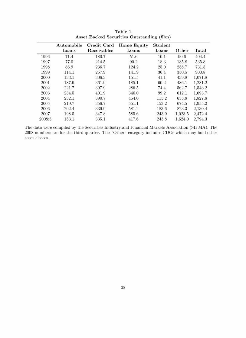
Table 1Asset Backed Securities Outstanding ($bn)

Automobile Credit Card Home Equity StudentLoans Receivables Loans Loans Other Total

1996 71.4 180.7 51.6 10.1 90.6 404.41997 77.0 214.5 90.2 18.3 135.8 535.81998 86.9 236.7 124.2 25.0 258.7 731.51999 114.1 257.9 141.9 36.4 350.5 900.82000 133.1 306.3 151.5 41.1 439.8 1,071.82001 187.9 361.9 185.1 60.2 486.1 1,281.22002 221.7 397.9 286.5 74.4 562.7 1,543.22003 234.5 401.9 346.0 99.2 612.1 1,693.72004 232.1 390.7 454.0 115.2 635.8 1,827.82005 219.7 356.7 551.1 153.2 674.5 1,955.22006 202.4 339.9 581.2 183.6 823.3 2,130.42007 198.5 347.8 585.6 243.9 1,023.5 2,472.42008:3 153.1 335.1 417.6 243.8 1,624.0 2,794.3

The data were compiled by the Securities Industry and Financial Markets Association (SIFMA). The2008 numbers are for the third quarter. The �Other�category includes CDOs which may hold otherasset classes.

28

Table 2Issuers and Entities in the ABX Index

Issuer Entities1 ACE Securities Corp. (DeutscheBank) 2005-HE72 Ameriquest Mortgage Securities 2005-R113 Argent Securities Inc. 2005-W24 Bear Stearns Asset Backed Securities, Inc. 2005-HE115 Countrywide Asset-backed Certi�cates 2005-BC56 First Franklin MTG Loan Asset Backed 2005-FF127 GSAMP Trust (GoldmanSachs) 2005-HE48 Home Equity Asset Trust (CSFB) 2005-89 JP Morgan Mortgage Acquisition Corp. 2005-OPT110 Long Beach Mortgage Loan Trust 2005-WL211 MASTR Asset Backed Securities Trust (UBS) 2005-NC212 Merrill Lynch Mortgage Investors Trust 2005-AR113 Morgan Stanley ABS Capital 2005-HE514 New Century Home Equity Loan Trust 2005-415 Residential Asset Mortgage Product Series (RFC/GMAC) 2005-EFC416 Residential Asset Securities Corp. (RFC/GMAC) 2005-KS1117 Securitized Asset Backed Receivables (Barclays) 2005-HE118 Soundview Home Equity Loan Trust (Greenwich) 2005-419 Structured Asset Investment Loan Trust (Lehman) 2005-HE320 Structured Asset Securities Corp. (Lehman) 2005-WF4

The data are from MarkIt and the securities represent the constituents of the ABX.HE 06-1 index.Ownership of the securities was con�rmed by MarkIt from the 8-K �lings of the registrants.

29

Table 3Weighted Average Deal Characteristics

ABX 60+ FICO LTV ARM IO Full Doc2006-01 11.94 634 80.36 81.75 32.13 58.712006-02 11.94 627 77.76 80.78 22.52 56.902007-01 5.48 626 79.21 76.84 15.64 57.57

The data were compiled by Nomura Fixed Income Research in April 18, 2007. All numbers arepercentages based on a weighted average of deals in the ABX indices. 60+ is the percentage ofmortgage holders who are 60 days or more delinquent. FICO is their credit score, LTV is the loanto value ratio, ARM is the percentage of �oating rate mortgages, IO is interest only mortgages, FullDoc refers to the whether full income documentation was provided by the borrower.

30

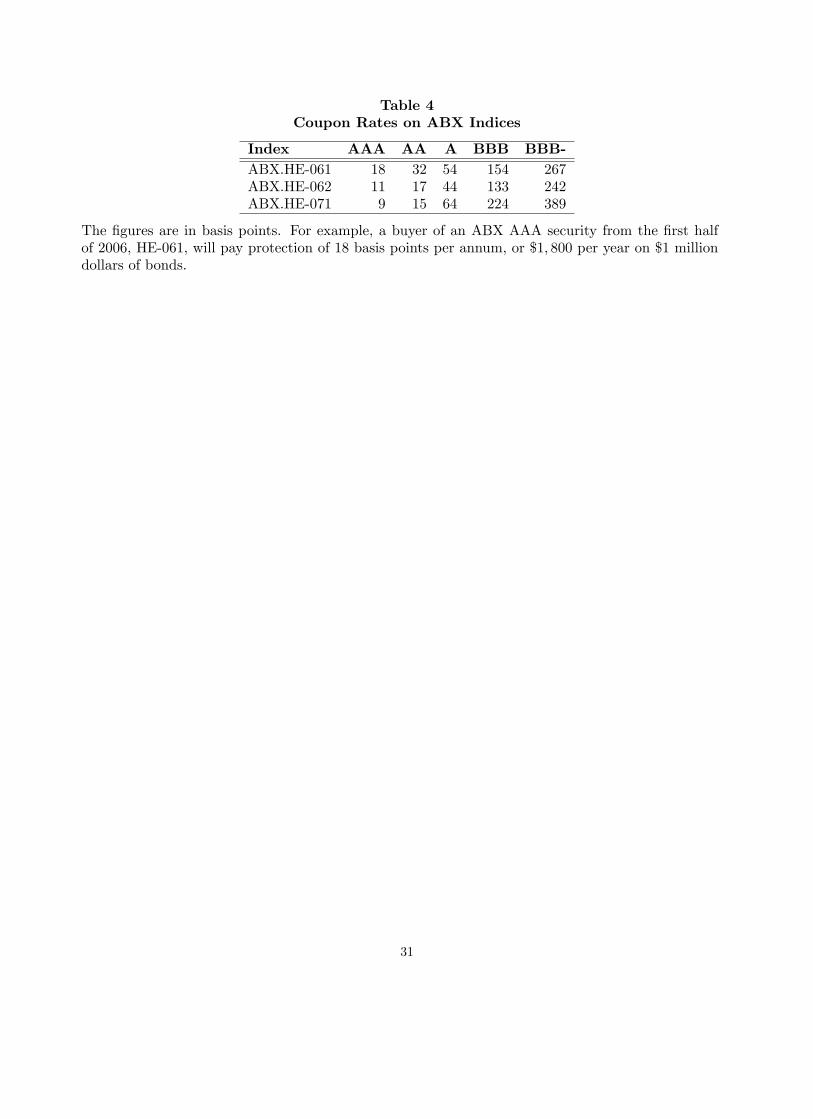
Table 4Coupon Rates on ABX Indices

Index AAA AA A BBB BBB-ABX.HE-061 18 32 54 154 267ABX.HE-062 11 17 44 133 242ABX.HE-071 9 15 64 224 389

The �gures are in basis points. For example, a buyer of an ABX AAA security from the �rst halfof 2006, HE-061, will pay protection of 18 basis points per annum, or $1; 800 per year on $1 milliondollars of bonds.

31

Table 5Implied Spread Computation

Tranche Coupon (bp) Price Duration Implied Spread (bp)AAA 9 82.72 5.07 350AA 15 49.57 3.70 1,378A 64 28.94 3.44 2,130BBB 224 19.86 3.02 2,878BBB- 389 18.94 2.75 3,337

The prices are from October 31, 2007 and are daily closes of the ABX.HE-071 roll with 100 rep-resenting par. Coupons are from Table 4. Duration estimates are from UBS and were �rst re-ported in Ashcraft and Scheurmann (2008). The implied spread is computed in basis points as100� (100� pt)=Duration+coupon.

32

Table 6Monte Carlo Experiments

Size5-min Daily

� RJ 5% 1% 5% 1%

0.9 0.00 0.292% 0.058% 0.000% 0.000%(0.51)% (0.23)% (0.00)% (0.00)%

0.2 0.00 0.870% 0.200% 0.000% 0.000%(0.97)% (0.43)% (0.00)% (0.00)%

0.025 0.00 0.328% 0.052% 0.000% 0.000%(0.57)% (0.23)% (0.00)% (0.00)%

Power5-min Daily

� E[J2] E[RJ ] J2 RJ 5% 1% J2 RJ 5% 1%

0.9 0.1 0.10 0.086 0.087 64.311% 53.414% 0.054 0.053 7.285% 2.726%(0.03) (0.03) (13.61)% (12.34)% (0.03) (0.03) (10.13)% (6.13)%

0.2 0.1 0.33 0.085 0.284 75.814% 69.932% 0.053 0.169 36.817% 25.420%(0.04) (0.08) (11.27)% (10.12)% (0.03) (0.08) (19.47)% (18.21)%

0.025 0.1 0.76 0.092 0.746 84.427% 82.400% 0.078 0.598 84.662% 79.917%(0.04) (0.08) (9.10)% (8.97)% (0.04) (0.10) (12.16)% (14.37)%

The table reports size and power comparisons of the intra-daily and daily estimators of jumps. Thedata generating process is (1)-(2) at a tick interval of 1-minute. I set � = 0, � = �0:5, � = 0:10, = 0:05; �J = 0:20, and �J = 1:40: In the size test, I set the jump frequency � to zero. In the powerexercise, I set � = 0:05dt which implies one jump every 20 days. In the size and power exercises,I vary the long run mean of volatility between � = 0:025 and � = 0:9: This lowers the percentagecontribution of the jump to total variance RJt from 76% to 10%: Standard errors are the standarddeviations across 500 Monte Carlo trials.

33

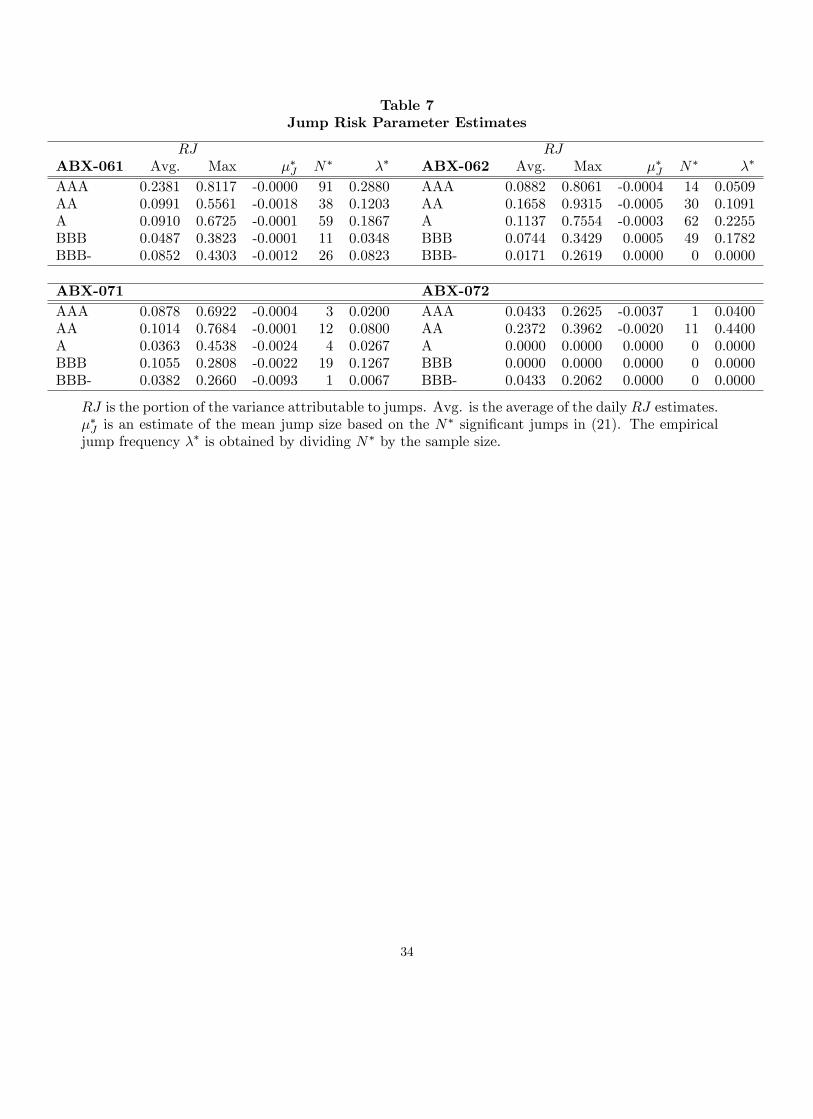
Table 7Jump Risk Parameter Estimates

RJ RJABX-061 Avg. Max ��J N� �� ABX-062 Avg. Max ��J N� ��

AAA 0.2381 0.8117 -0.0000 91 0.2880 AAA 0.0882 0.8061 -0.0004 14 0.0509AA 0.0991 0.5561 -0.0018 38 0.1203 AA 0.1658 0.9315 -0.0005 30 0.1091A 0.0910 0.6725 -0.0001 59 0.1867 A 0.1137 0.7554 -0.0003 62 0.2255BBB 0.0487 0.3823 -0.0001 11 0.0348 BBB 0.0744 0.3429 0.0005 49 0.1782BBB- 0.0852 0.4303 -0.0012 26 0.0823 BBB- 0.0171 0.2619 0.0000 0 0.0000

ABX-071 ABX-072AAA 0.0878 0.6922 -0.0004 3 0.0200 AAA 0.0433 0.2625 -0.0037 1 0.0400AA 0.1014 0.7684 -0.0001 12 0.0800 AA 0.2372 0.3962 -0.0020 11 0.4400A 0.0363 0.4538 -0.0024 4 0.0267 A 0.0000 0.0000 0.0000 0 0.0000BBB 0.1055 0.2808 -0.0022 19 0.1267 BBB 0.0000 0.0000 0.0000 0 0.0000BBB- 0.0382 0.2660 -0.0093 1 0.0067 BBB- 0.0433 0.2062 0.0000 0 0.0000

RJ is the portion of the variance attributable to jumps. Avg. is the average of the daily RJ estimates.��J is an estimate of the mean jump size based on the N

� signi�cant jumps in (21). The empiricaljump frequency �� is obtained by dividing N� by the sample size.

34

Table 8(a)Subprime News Flow: Dec. 2006-August 2007

Date News BBC JEC PIMCO20061228 OwnIt Mortgage Solutions �les for bankruptcy X

20070207 Senate has hearings on subprime lending X

20070212 ResMae Mortgage �les for bankruptcy X

20070220 Nova Star has surprise loss X

20070222 HSBC �res head of US mortgage business after $10.5bn loss X

20070302 Fed announces draft regulations for subprime X

20070308 DR Horton warns of huge losses X

20070308 New Century stops making loans X X

20070312 New Century shares halted X

20070316 Accredited Home Lenders sells $2.7bn in loans X

20070320 People�s Choice �les for bankruptcy X

20070327 Bernanke �likely to be contained� X X

20070402 New Century �les for bankruptcy X X X

20070406 American Home Mortgage writes down risky mortgages X

20070418 Freddie announces plans to re�nance $20bn in subprime X

20070424 Sales of existing homes fall 8.4%, sharpest in 18 years X X

20070503 GMAC loses heavily in subprime X

20070503 UBS closes subprime lending arm X

20070509 Fed does not change rates X

20070517 Fed does not see broader economic impact X

20070612 Foreclosure �lings surge 90% year over year. X X

20070614 Frank says Fed could lose mortgage regulatory authority X

20070614 News emerges about large liquidations at Bear X

20070614 Goldman reports �at pro�t X

20070622 Bear Stearns $3.2bn hedge fund bail out X X X

20070629 Bear �res head of asset management X

20070710 S&P and Moody�s negative ratings $12bn in subprime X X

20070713 GE decides to sell WMC subprime business X

20070718 Bear : investors will get little money back X X X

20070719 Fed comments shake global shares X X

20070720 Bernanke warns subprime crisis could cost up to $100bn X

20070724 Rising default hit pro�ts at CFC X

20070726 Bear Stearns seizes assets. Shares fall 4.2%, largest in �ve year. X

20070727 Worries about subprime hammer global stock markets X

20070730 Germany�s IKB bailed out X

20070731 Bear Stearns stops withdrawls from third fund X X

20070731 Home prices show 18th consecutive decline in growth rate X

20070803 Shares fall heavily on fears of credit crunch X

20070806 American Home Mortgage �les for bankruptcy X X

20070807 Fed leaves rates at %5.25 X

BBC is the British Broadcasting Company, JEC is the Joint Economic Committee of U.S. House ofRepresentatives, and PIMCO is from the Paci�c Investment Management Co.

35

Table 8(b)Subprime News Flow: Aug.-November 2007

Date News BBC JEC PIMCO20070809 Coordinated intervention by ECB, Fed and Bank of Japan X X

20070809 AIG warns defaults spreading beyond subprime X

20070809 BNP Paribas suspends 3 funds X X

20070810 ECB provides extra 61bn in Euros. Fed pledges overnight money X

20070810 Global markets pressure. Worst day on FTSE in 4 years X

20070813 ECB pumps 47.7bn in Euros into money markets X

20070813 Goldman provides $3bn support for hedge fund X

20070813 Aegis Mortgage �les for bankruptcy X

20070816 CFC draws entire 11.5bn credit line X X X

20070817 Fed cuts discount rate by 50 basis points X X X

20070820 CFC cuts jobs X

20070823 CFC get $2bn cash infusion from BAC X

20070828 German Sachsen Landesbank sold under threat of collapse X

20070831 Bernanke at Jackson Hole says US will act as needed X

20070903 German IKB records $1bn loss X

20070904 Bank of China reveals $9bn in subprime losses X

20070904 Overnight bank lending dries up X

20070906 ECB injects fresh cash into market X

20070911 Trichet says EU economy sound X

20070914 Northern Rock shares plummet after BofE rescue plan announced. X

20070914 Merrill signals mortgages will hurt 3Q earnings X

20070917 NovaStar eliminates its REIT

20070917 Merill Lynch job cuts at First Franklin X

20070918 Fed cuts interest rates to 4.75% X X

20070918 Impac Mortgages closes

20070920 Bernanke says subprime losses higher than expected X

20070920 Goldman makes pro�ts betting MBS will fall X

20070921 HSBC closes Decision One X

20071001 UBS reveals $3.4bn loss X X

20071001 Greenspan says housing crisis far from over

20071005 Merrill reveals $5.6bn subprime loss X

20071010 Bush administration Hope Now X

20071015 Citi writes down additional $5.9bn X X

20071016 Bernake: subprime crisis and housing slump will be drag X X

20071018 S&P cuts grades on 23.3bn of loans X

20071024 Merrill Lynch announces $7.9bn writedown X X

20071030 Merrill O�Neal resigns X

20071031 Deutsche Bank reveals $3bn writedown X

20071031 Fed delivers second rate cut X X X

20071101 CFSB writes down $1bn X

BBC is the British Broadcasting Company, JEC is the Joint Economic Committee of U.S. House ofRepresentatives, and PIMCO is from the Paci�c Investment Management Co.

36

Table 9ABX Index News Regressions

Tranche D1;t�1 D2;t�1 Stat.AAA -0.0002 -0.0003 Coe¤

(-8.99) (-10.74) (t-stat)

0.4727 0.5622 R2

AA -0.0032 -0.0036 Coe¤(3.11) (2.15) (t-stat)

0.1897 0.0896 R2

A -0.0005 -0.0012 Coe¤-4.2087 -4.3029 (t-stat)

0.2237 0.2319 R2

BBB 0.0000 0.0000 Coe¤0.0000 0.0000 (t-stat)

0.0000 0.0000 R2

BBB- -0.0013 -0.0026 Coe¤3.9656 4.0664 (t-stat)

0.5250 0.5260 R2

These are estimates of the e¤ect of news on ABX index jump risk using the speci�cation (24) in thetext. D1;t is a 5-day moving sum of the number of news stories in the BBC, JEC, and PIMCOtimelines in Table 8. D2;t is the number of news timelines that carried a particular story on that day.I estimate the model on days when jump risk is statistically signi�cant.

37

Table 10CME Housing Futures Jump Risk Parameter Estimates

RJContract Avg. Max ��J N� ��

f1 0.4071 1.0000 0.0013 212 0.6709

f12 0.4617 1.0000 0.0012 221 0.6994

f1 is the 1-month ahead contract, and f12 is the 12-month. RJ is the portion of the varianceattributable to jumps. ��J is an estimate of the mean jump size based on the N

� signi�cant jumps in(21). The empirical jump frequency �� is obtained by dividing N� by the sample size.

38

Table 11CME Housing Futures News Regressions

Contract D1;t�1 D2;t�1 Stat.f1 1.5669 1.3200 Coe¤

(-2.57) (-2.07) (t-stat)

0.0259 0.0153 R2

f12 0.2271 -0.1547 Coe¤(-0.36) (-0.27) (t-stat)

-0.0040 -0.0042 R2

These are estimates the e¤ect of news on housing futures jump risk using the speci�cation (24) in thetext. f1 is the 1-month ahead contract, and f12 is the 12-month. Coe¢ cient estimates are �104.D1;t is a 5-day moving sum of the number of news stories in the BBC, JEC, and PIMCO timelines inTable 8. D2;t is the number of news timelines that carried a particular story on that day. I estimatethe model on days when jump risk is statistically signi�cant.

39

Table 12Monte Carlo Analysis of Cojumps

� = 0:1 � = 0:5�J 5% 1% 5% 1%

0:50 92:532% 90:442% 90:103% 88:502%(19:68)% (23:25)% (22:73)% (25:13)%

0:75 88:810% 87:088% 87:710% 86:118%(17:99)% (19:54)% (20:15)% (21:24)%

The table reports rejection frequencies for the daily cojump statistic (26). The data generatingprocess is a bivariate version of (1)-(2) at a tick interval of 1-minute. I set � = 0, � = �0:5, � = 0:10, = 0:05; � = 0:05dt, �J = 0:20, and �J = 1:40: I vary the long run mean of volatility between� = 0:1 and � = 0:5 and the correlation of jump occurrence from 0:5 to 0:75. Standard errors arethe standard deviations across 500 Monte Carlo trials.

40

Table 13Cojump News Regressions

Tranche D1;t�1 D2;t�1 Stat.AAA -4.0632 -3.1544 Coe¤

-(4.42) -(3.99) (t-stat)

0.4263 0.3736 R2

BBB- -0.4364 -0.3558 Coe¤-(1.55) -(2.33) (t-stat)

0.0549 0.1553 R2

These are estimates the e¤ect of news on cojump risk for the ABX-061 tranches paired with the12-month CSI composite futures using the speci�cation (31) in the text. Coe¢ cient estimates are�106. D1;t is a 5-day moving sum of the number of news stories in the BBC, JEC, and PIMCOtimelines in Table 8. D2;t is the number of news timelines that carried a particular story on that day.I estimate the model on days when cojump risk is statistically signi�cant.

41

Table 14Empirical Model of ABX Jump Risk

Tranche Constant J�1;z;t�1 J2�1;z;t�1 J�2;z;t�1 (f12t�1 � f1t�1) R2

AAA -0.2446 0.1112 -441.6708 0.0508 -0.0199 0.0756-(2.41) (0.34) -(0.54) (2.13) -(2.29)

AA -0.2476 0.6340 -468.7428 -0.0142 -0.0214 0.8483-(1.28) (1.52) -(13.40) -(0.20) -(1.27)

A -0.8450 -0.2187 -1,156.9378 0.0363 -0.0670 0.5884-(2.99) -(0.95) -(4.87) (0.61) -(3.14)

BBB -1.1830 -0.0927 -1,595.0460 -0.0267 -0.1030 0.3103-(0.94) -(0.16) -(0.88) -(0.15) -(1.20)

BBB- -9.9029 -0.1508 57.5454 1.0907 -0.6873 0.8393-(9.91) -(0.56) (1.21) (4.27) -(9.42)

The table contains estimates of the predictive ABX jump risk model (32): J�1;z;t�1 is the lagged ABXjump risk, J2�1;z;t�1 is the lagged squared ABX jump risk, J

�2;z;t�1 is the lagged jump risk from the CME

housing futures, and (f12t�1 � f1t�1) is the slope of the housing futures curve out one year. Coe¢ cientestimates on the futures curve are �104. t-ratios are in parentheses. The sample period is August2006 to November 2007.

42

Table 15VaR Estimates

Tranche !�2 !�2;t #r� < V aR0:05 #r� < V aR

0:05

#J21;z > 0

AAA �0:3529% 0.1112 26 13

BBB- �2:5650% 0.6340 45 10

The table reports daily 95% con�dence level V aR for an ABX and futures portfolio. The static hedgeratio is given by (34) and the dynamic hedge ratio by (36). The third column reports the numberof exceedences of V aR0:05 in the data, and the fourth column reports the number of times theseexceedences occur on days with signi�cant jumps in the ABX.

43

Figure 1Prices on A Rated Tranches of ABX.HE 2006-1

May 2006-November 2007

The data are daily closing prices on the ABX.HE indices for the �rst half roll of 2006.

44

Figure 2Prices on B Rated Tranches of ABX.HE 2006-1

May 2006-November 2007

The data are daily closing prices on the ABX.HE indices for the �rst half roll of 2006.

45

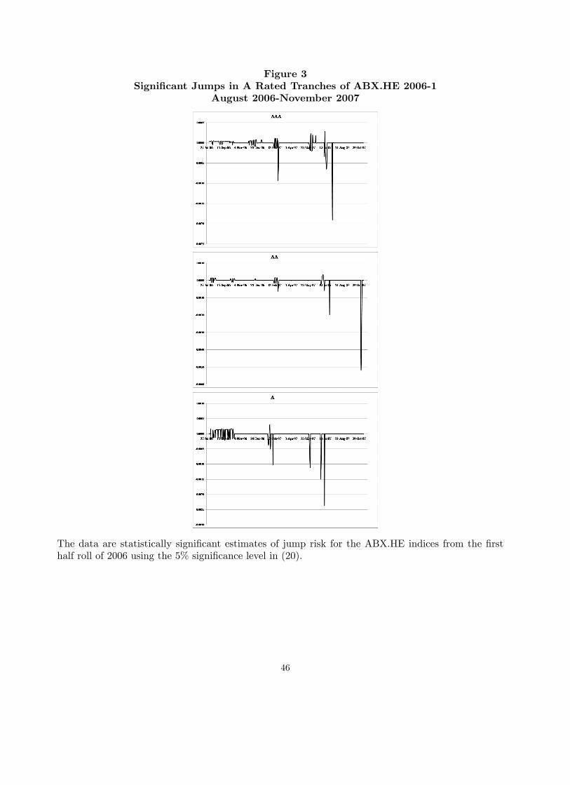
Figure 3Signi�cant Jumps in A Rated Tranches of ABX.HE 2006-1

August 2006-November 2007

The data are statistically signi�cant estimates of jump risk for the ABX.HE indices from the �rsthalf roll of 2006 using the 5% signi�cance level in (20).

46

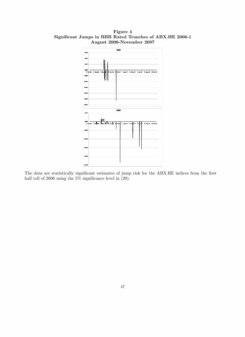
Figure 4Signi�cant Jumps in BBB Rated Tranches of ABX.HE 2006-1


The data are statistically signi�cant estimates of jump risk for the ABX.HE indices from the �rsthalf roll of 2006 using the 5% signi�cance level in (20).

47

Figure 5Jump Risk Of CME Composite CSI Housing Futures


The data are estimates of jump risk (18) for the CME CSI composite housing futures for the nearmonth f1 and one year f12 expirations,

48

Figure 6Cojump Risk Of ABX Housing Futures


The �gures plot signi�cant cojump risk (29) for the ABX.HE 06-1 and the 12-month ahead CMECSI composite housing futures.

49

Figure 7VaR Estimates of Hedged ABX and Futures Portfolio


The �gures plot the value-at-risk for static (35) and dynamically hedged (37) portfolios in theABX.HE 06-1 and the CME CSI composite housing futures.

50

Documents

Jump and Cojump Risk in Subprime Home Equity Derivatives · Jump and Cojump Risk in Subprime Home Equity Derivatives Bruce ... mergers of Bear Stearns with JP ... power as long as