AD-A283 962 P E NUMBER u -D4

ll NlA DTIC C3 ELECTE 0JUL 0 81994i

F .COPYl0 Frequency Response of Multipass

Shell-and-Tube Heat Exchangers

LEWIS ISCOLResearch Fellow, Department ofOwmcol Enginerg, University LIBRARY COPYof Wisconsin, Madison, Wis.

X J. ALTPETER APR 9 'E9Professor of Chemical En ganereUniversity of Wisconsin,Madison, Wis.

Transfer functiomn are derived for exchangers with one shell pasn and 2n

tube passes. It is shown how the method of derivation may be generalized

to apply to exchangers with an arbitrary number of shell-and-tube passes.

0 Distributed thermal capacity in pipe walls may be introduced as such, lumped,

or neglected entirely.• • '-n ýI~oveP

~This docum"I' r~.c3z ,I,, ipp0Ito' pubU*C :e6eOSO ad sole;

dkstribut1On I~?ME

94-20124liII 11 111 I|liiil

S946 29 16t7wr presetation at the Instrumgents and Regulator Cmmfereumc Oevelagud, Ohioa,March fl-Apr 2, 1959, of Mhe American Society of Mechanical EngMnee Mana,

"N AMIEICAN SOCIfTY OF MiCHANICAL IOINUNM scpt received a t ASME Headquarters, January , 1509.

W410 39th 501w, New Ywh U, N. Y. iWritten diacualson on this paper will be accepted up to May 4, 10L

Copla will be available until January I, 101.

HIOT PHOTOGRItH

Frequency Response of Multipass Shelland-Tube Heat Exchangers

LEWIS ISCOL L. L ALTPETER

NOMENCLATURE

The following nomenclature is used in the paper:

a, = (dl)w.T C1.

a_ = hoA (dl)

Ws, Ci1

A = heat transfer area per pass (sq ft)

b, = hT A (dl)c-._P F. vq

hV A •.- ,-,

7C..y,. VK

C = heat catpacity (BTU/lb FO)

C, C' = arbitrary constants (dl)

d = thermal diffusivity of pipe wall (sq ft/hr)

D = intermediate parameter (dl)

e = 2.7182818... (dl)

E = intermediate parameter (*F)

f = intermediate parameter (dl)

F = cross sectional area of metal in pipe wall (sq ft)

g = intermediate parameter (dl)

h = heat transfer coefficient (BTU/hr sq ft F')

k = thermal conductivity (BTU/hr ft FO)

K = intermediate parameter (dl)

L = tube length per pass (ft)

m = number of shell passes (dl)

2

M - intermediate parameter (dl)

n - number of tube passes in each direction per shell pass (dl)

N = intermediate parameter (dl)

p = intermediate parameter (dl)

P = heat transfer perimeter of pipe (ft)

q = constant of integration (OF)

r ' (dl)

R = intermediate parameter (dl)

s Laplace transform variable (dl)

S = shellside fluid temperature (*F)

1 Laplace transform of S (OF)

t = time (hr)

T = tubeside fluid temperature (OF)

T= Laplace transform of T (OF)

U = overall heat transfer coefficient (BTU/hr sq ft FO)

v = fluid velocity (ft/hr)

V, V = definite integrals (OF)

w = fluid flow rate (lb/hr) Accesion For

NTIS CRA&IW = pipe wall temperature (OF) DTIC TABUnannou -cedI= Laplace transform of W (*F) Justification

x = axial distance along exchanger (ft) By

y = axial distance along exchanger (dl) Distribution14

Z = intermediate parameter (dl) Aojia•m ,

•x=U A (dll)

U A (dl)W. elf

2.

L' d (dl)

Y. h- (dl)k

Y2. :f (dl)k

= pipe wall thickness (ft)

= intermediate parameter (dl'

= root of auxiliary cubic (dl)

e = time (dl)

A = radial distance through pipe wall (ft)

= intermediate parameter (dl)

= density (lb/cu ft)

= radial distance through pipe wall (dl)

A , Al = dummy variables

V, = intermediate parameter (dl)

Subscripts:

i = ordinal isumber of shell pass

j = ordinal number of tube pass within a particular shell pass

Q = summation index

R = reference

S = shellside

T = tubeside

W = pipe wall

As usual the use of an independent variable as a subscript of

a dependent variable indicates partial differentiation,

@Tas T = - - "

x 5

I

INTRODUCTION

A multipass shell and tube exchanger may be described

by a set of partial differential equations similar, in many

respects, to those describing a counterflowk•-)I or one side

lumpec#) exchanger. This set of equations may be thought of

as constituting a mathematical model of the exchanger.

Models of varying degrees of complexity may be constructed

for the same exchanger. In this paper models are first

constructed which neglect the heat capacity of tube walls.

Refinements are then made which allow the walls to be

introduced as either lumped or distributed thermal capacity.

The models presented herein are quite formidable of aspect,

involving the definition of many sets of intermediate parameters.

It should be borne in mind that the question which must be

answered regarding the feasibility of use of a given model

is not, "How complicated is the model?" but, "How much does

it cost to extract the desired information from the model?".

The desired information is here the frequency response

characteristics of the exchanger. This information may be

particularly easily extracted if an explicit expression is

obtainable for the transfer function. Such an expression

is obtainable for the models considered. In fact, it is the

object of this paper to show how such explicit transfer

functions may be obtained.

The evaluation at a particular frequency of a transfer

function of the complexity here considered takes on the order

of 15 seconds on an intermediate speed digital computer and so

I Numbers in parentheses designate References at end of paper.

S• m m | a 5

S(tx) j4 T(t,x) ------ a-

,o() (a -L

ORIENTATION I

S(tx)

S~Tit,x)

X-o (b) x-L

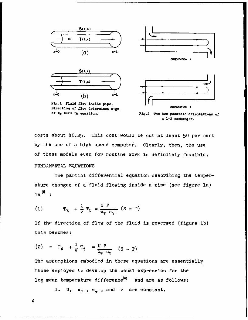
Fla.l Fluid flow inside pipe.Direction of flow determines sign ORIENTATION 2of Tx term in equation. Pig.2 The two possible orientations of

a 1-2 exchanger.

costs about tO.25. This cost would be cut at least 50 per cent

by the use of a high speed computer. Clearly, then, the use

of these models even for routine work is definitely feasible.

FUNDAMENTAL EQUATIONS

The partial differential equation describing the temper-

ature changes of a fluid flowing inside a pipe (see figure la)

is

i U P (S-T

(1) T-A + I Tt w= (S - T)

If the direction of flow of the fluid is reversed (figure lb)

this becomes:

(2) - TX +--1 Tt U P (S - T)v w T C -

The assumptions embodied in these equations are essentially

those employed to develop the usual expression for the

log mean temperature differenceP) and are as follows:

1. U, wT , cT , and v are constant.

6

2. Plug flow prevails.

3. No temperature gradients exist in the fluid other

than in the axial direction.

4. No partial phase changes take place in the system.

Equations (1) and (2) are made dimensionless by the introduction

of new space and time variables.

(3) Y xt vI•

(4)e = -

L

Using (3) and (4), (1) becomes:

v1R

(5) T3 + TV = o ,(S - T)

Each pass of a multipass exchanger is described by an equation

similar to (5). These equations together with appropriate

boundary conditions constitute one model of the exchanger.

THE 1 - 2n EXCHANGER

Two orientations of a 1-2 exchanger are possible (see

figure 2). For each orientation there are four possible

temperature forcing transfer functions. Forcing may be

applied on either the tube or shell side, and the response

may be taken on either side.

Transfer functions will be derived for the case of

orientation 1, forcing on the tube side, with response on

either side. Disturbances frequently take the path, forcing

on the tube side, response on the tube side. Corrective

action, however, frequently involves flow forcing which is

not here considered. The other six possible temperature

7

forcing transfer functions may be derived by procedures very

similar to the oneS to be demonstrated.

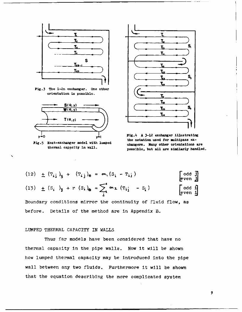
The equations for the l-2n exchanger (see figure 3)

are, in dimensionless form:

(6) (TJ) + (T)9e = c,(S - T11) J = 1,3,5,...2n-1

(7) -(Tj) + (T1) = -,(S - Ti) J = 2,4,6,...2n

(8) s• + r s8 =+ S (T• -S)

Note that tubeside velocity is chosen as reference velocity.

The additional assumption is made that the area of each pass

is the same. Boundary conditions are:

(9) Tý (t,o) = T•. (t,0) J = 3,5,7,...2n-1

(10) Tj (tl) = Tj. (t,i) j = 2,4,6,...2n

(11) S(t,o) = 0

The solution is carried out in detail in Appendix A.

THE GENERAL MULTIPASS SHELL AND TUBE EXCHANGER (m - 2mn)

Under the additional mild restriction that there be no

heat transfer between different shell passes (also a usual

steady state assumption ) it is possible to derive explicit

transfer functions for the general multipass shell and tube

exchanger having m shell passes and 2n tube passes per. shell

pass. The notation is illustrated by figure 4. When two

subscripts are used the first always refers to the number of

the shell pass. The equations take the form:

8

IZ LLk Ts I•

T4T

T, To

orie1ntio is Aoneharla

yT3I

T.l ~ ~ ~ w(e, Y)I'-- ", -_ .•

y-o jl, Fg.4. A 3-12 exhage ilustratin

the notation used for multipass ex-Pi .5 Heat-exchanger model with lumped changers. Many other orientations are

therual capacity in wall. possible, but all are similarly handled.

(12) + (T1,•)j + (Tj j )e = - (Si - Tij) vdde[even

(13) + (Sj ) + r (Sj) =5CWR.; (Til Si s~odd~Leven

Boundary conditions mirror the continuity of fluid flow, as

before. Details of the method are in Appendix B.

LUMPED THERMAL CAPACITY IN WALLS

Thus far models have been considered that have no

thermal capacity in the pipe walls. Now it will be shown

how lumped thermal capacity may be introduced into the pipe

wall between any two fluids. Furthermore it will be shown

that the equation describing the more complicated system

may be reduced to the form previously considered.

The system of figure 5 has been described by the equations:

(14) T 1 + To 01C, (S -T)

(15) S" + r S,,= w(T -S)

It may also be described by the set:

(16) T +T = a, (W -T)

(17) S3 + r Se =a (W- S)

(18) We b, (T -W) + bx (S - W)

Transforming and rearranging (18) one obtains:

bf

(19) 7 - _ +s + b, + b s + b, + b2

Using this expression for 7 in the'transforms of (16) and (17),

a,, b, a, b.(20) + Ls+a, T =.b

s+b. + s+ b + b•

(a2 b,,.bL a 7 bi

s+b, +b, s+ b% + ba.

Equations (20) and (21) are of the same form as the transforms

of (14) and (15), but with different constants. The solution

from this point on is the same as before.

The treatment for the case of a wall in contact with

a single fluid (as a shell wall) is similar. It should

be noted that in a single exchanger the thermnl cnpacity' of

10

some walls may be neglected, the thermal capsclty of' other

walls lumped, and the capacity of still other walls treated

in distributed fashion as will be described below.

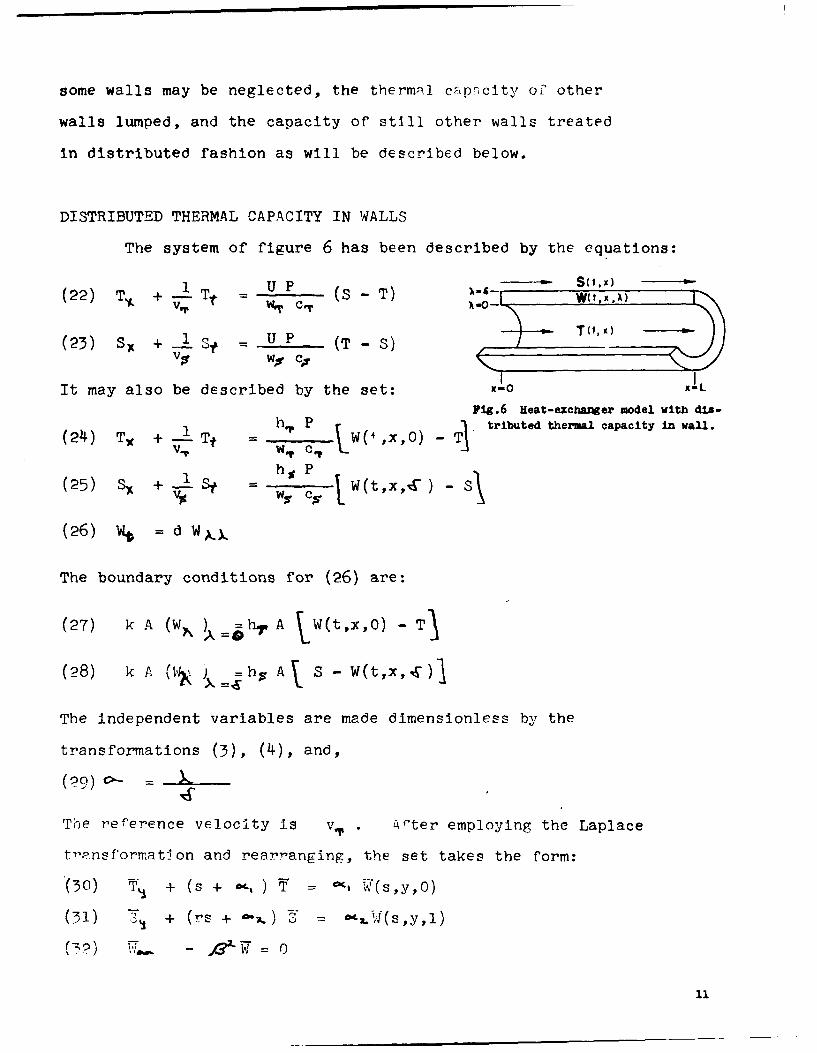
DISTRIBUTED THERMAL CAPACITY IN WALLS

The system of figure 6 has been described by the equations:

S U P (.- S(t.x)(22) T* + Tt (S-T) v A)

(23) +1 Sf P U P (T - S)

It may also be described by the set: X-o x!L

PFg.6 Heat-excbanger model with diB-

(24) Tx +-T =h.r P [ T tributed thermal capacity in wall.

S• , W(t ,x,O-) -S

(25) S, + St = h$t 6-w% cr CO~

(26) Wt =d WX,

The boundary conditions for (26) are:

(27) k A (Wh =h,A VW(t,x,O)- T-

(28) k A ('•).=h AV S - W(t,x,,-1

The independent variables are made dimensionless by the

transformations (3), (4), and,

(?9) c-- = L

The reference velocity is v. . 'ter employing the Laplace

trpnsformation and rear-anging, the set takes the form:

(30) T + (s + -- ) Y = , '(s,y,0)

(31) • + (r s + 9-- . --- • (s,y,1)

11

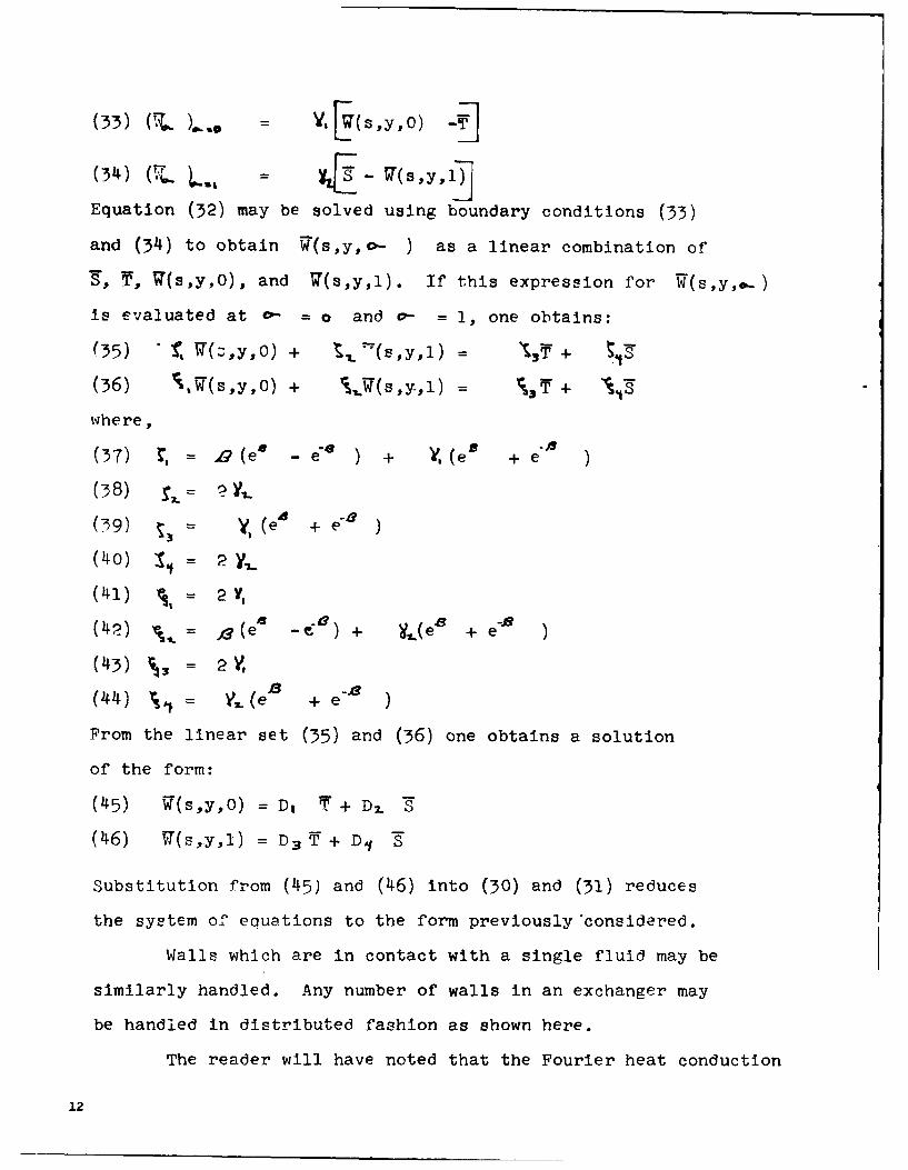
Equation (32) may be solved using boundary conditions (33)

and (34) to obtain !(s,y,>- ) as a linear combination of

7, 7, 7(s,y,O), and V(s,y,l). If this expression for 74(s,y,.-)

is evaluated at - = o and v- 1, one obtains:

(35) V(Z,y,0) + (js,y,l) = sf+ +

(36) %,,(s,y,o) + i.3(s,y,l) = ,y + A'

whe re,

(37) , (ee - e" ) + X,(es + e )

(38) Y,

(39) V =(ee + e"'(40) 2• yj_ F

(41) , = 2 Y,(42) r% f3 /(e- -,6) + V,.(ee + e- )

(43) Y,

(4 )V= .(eI + e )

From the linear set (35) and (36) one obtains a solution

of the form:

(45) W(s,y,o) = D, T + D2. S

(46) 71(s,y,l) = D 3 T + D.

Substitution from (45) and (46) into (30) and (31) reduces

the system of eauations to the form previously considered.

Walls which are in contact with a single fluid may be

similarly handled. Any number of walls in an exchanger may

be handled in distributed fashion as shown here.

The reader will have noted that the Fourier heat conduction

12

equation is.s ed in rectangular coordinates rather than

cylindr.'cal, as is strictly required. .The error introduced

is not large and is outweighed by the convenienne of being

able to obtain an explicit transfer function in terms of

the elementary functions.

It should be noted that models in the literature of

counterflow(t', , parallel flowkiD) , and one side lumpej31

exchangers may be refined and thus undoubtedly brought into

better agreement with experimental work by the addition of

distributed thermal capacity in the pipe walls, as provided

for here.

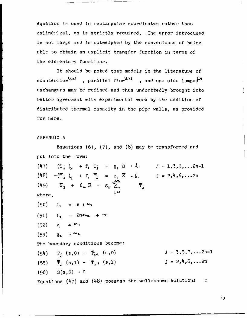
APPENDIX A

Equations (6), (7), and (8) may be transformed and

put into the form:

(47) (TF )• + f, Tj = g J = 1,3,5,...2n-1

(48) -(T )• + f, Ti = g' S -7 J = 2,4,6,...2n

(49) 7 + f " =1 a

where,

(50) f, =s +

(51) f_ = 2not-,. + rs

(52) g =,

(53) g27 = •1-

The boundary conditions become:

(54) Ti (s,O) = Tý_, (s,O) J = 3,5,7,...2n-1

(55) Tj (s,l) = T30 (s,l) j = 2,4,6,...2n

(56) '§(sO) = 0

Equations (47) and (48) possess the well-known solutions

13

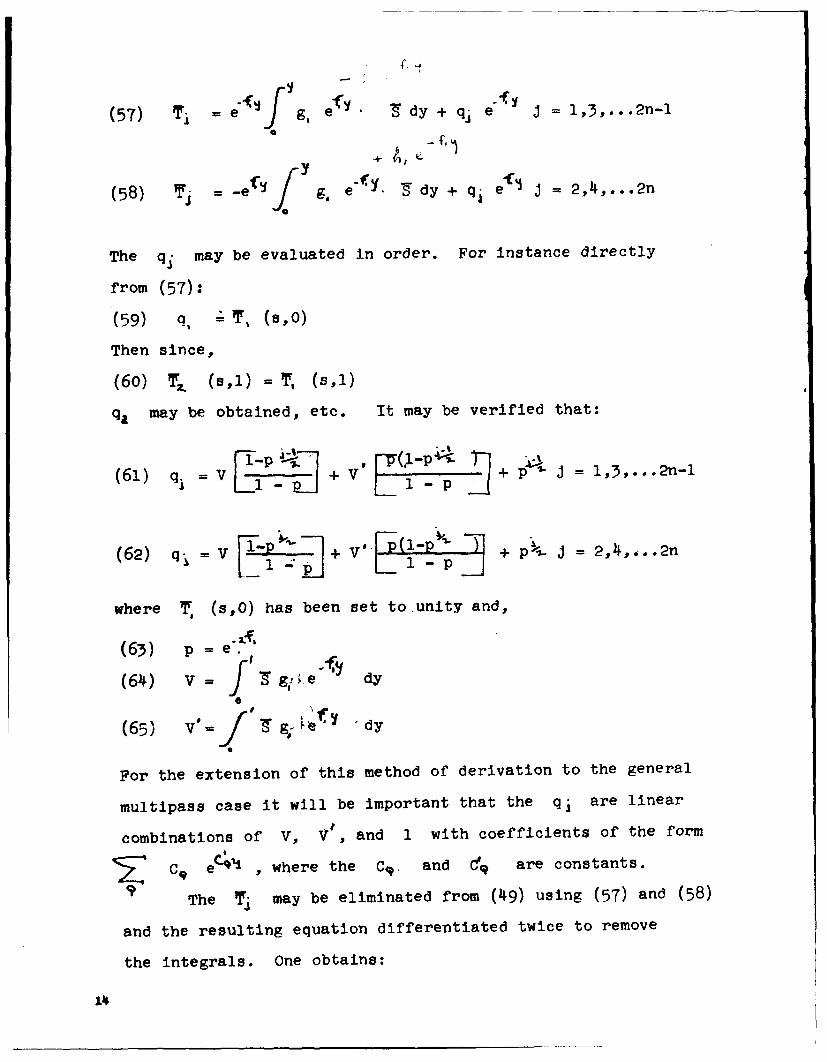
(57) e . e fl dy + q e J 1,3,...2n-l

m / ~Y , e..•

(58) --eflJ g, e dy + q, 3l = 2,4,...2n

The qj may be evaluated in order. For instance directly

from (57):i ~ ~(59) , ,(so

Then since,

(60) 7r (s,1) = , (s,l)

q. may be obtained, etc. It may be verified that:

(61) q = V jj + V + p- j = 1,3,...2n-1

(62) q- = V .. 5 + v j - + p. j = 2,4,a,.2n

where , (s,O) has been set to unity and,

(63) p = e'. I

(64) V = f1 g1 .,e dy

(65) V-= Lb dy

For the extension of this method of derivation to the general

multipass case it will be important that the q are linear

combinations of V, VI, and 1 with coefficients of the form

"Z C, eC.Al , where the Cq. and 49 are constants.

9 The I may be eliminated from (49) using (57) and (58)

and the resulting equation differentiated twice to remove

the integrals. One obtains:

114

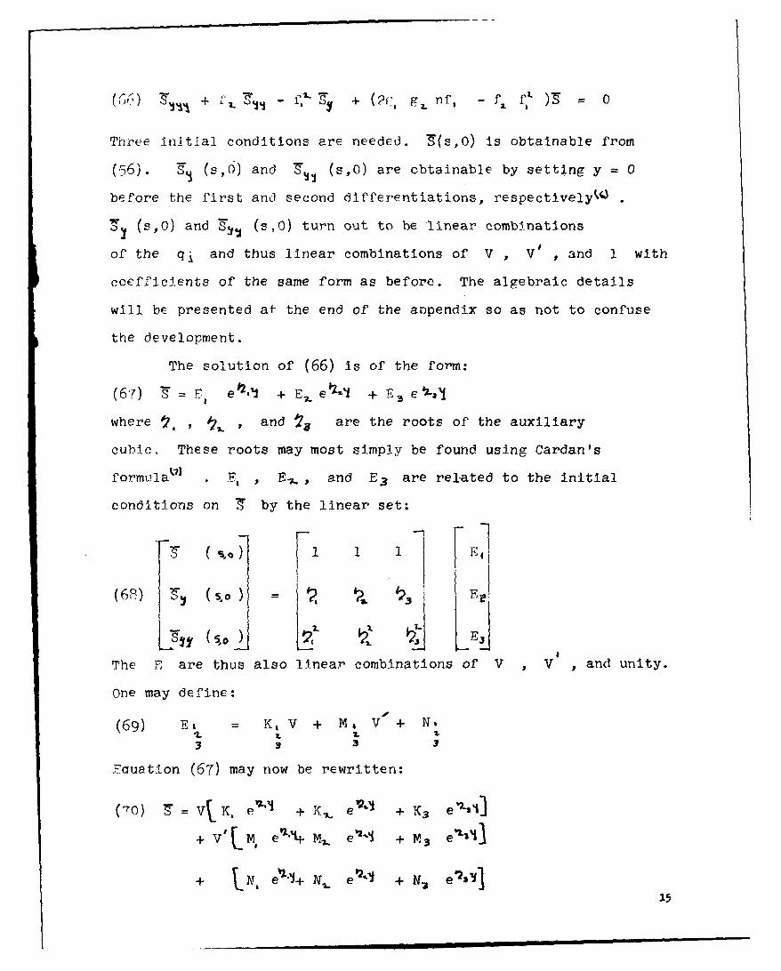
(+f "94 -~Z f. S1 + n f.. ff, 7 0

Three initial conditions are needed. '(s,O) is obtainable from

(56). S-- (s,O) and ' (s,O) are obtainable by setting y - 0

before the first and second differentiations, respectively%)

• (s,O) and S" (s,O) turn out to be linear combinations

of the q and thus linear combinations of V , , and I with

coefficients of the same form as before. The algebraic details

will be presented at the end of the anpendix so as not to confuse

the develonment.

The solution of (66) Is of the form:

(6 7 = F e + E - e -1 + E,3 e "-&I

where , , , and J, are the roots of the auxiliary

cubic. These roots may most simply be found using Cardan's

formula'I El E., and E 3 are rel-ated to the initial

conditions on . by the linear set:

(6R) -9 (5,0 =2 E7. It

The T are thus also linear combinations of V , V , and unity.

One may define:(69) E = K, V + M4 V + N.

1- z. 21

3 3 3 3

.,'auation (67) may now be rewritten:

(70) 'g = V K. Pv' + X , e 9" + K3 e'~~

+ V'FMe'-li+ MI. 0-4i + M 3 3i

+ [hj e*'-I+ I-. e12t"1 + N* e 123

15

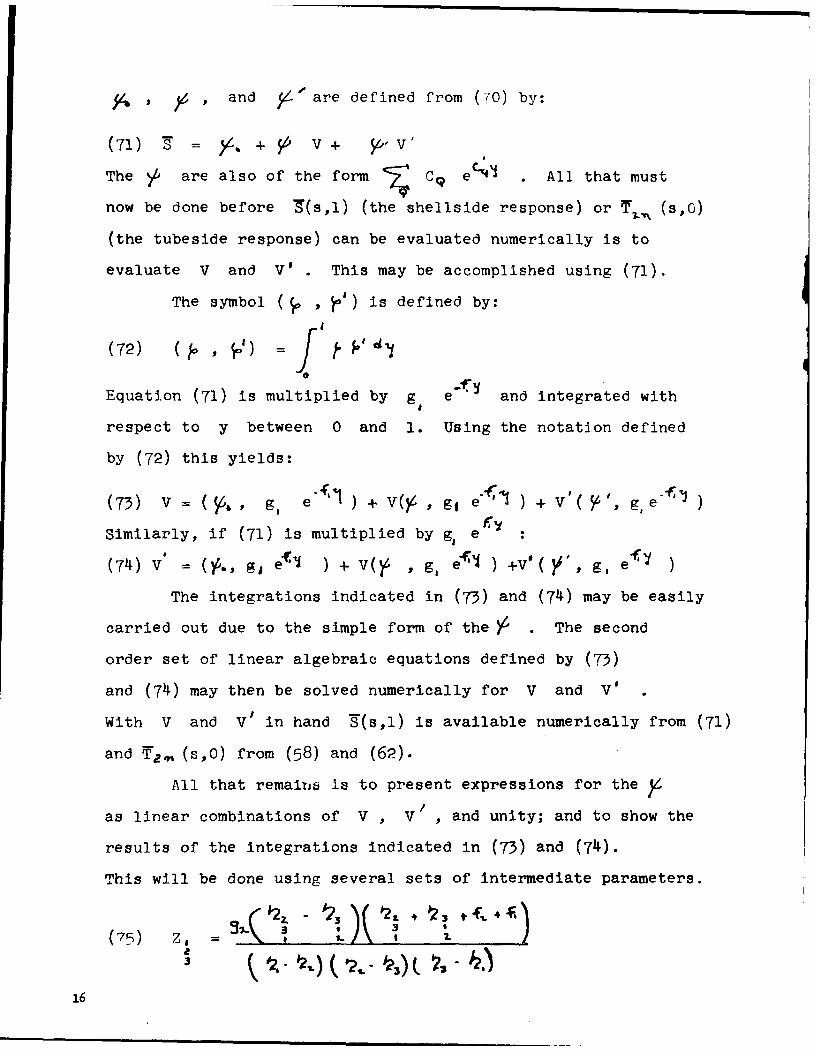
, and i/are defined from (t'O) by:

(71) C - I+ v + 5 , v 'The >I are also of the form C. e All that must

now be done before §(s,l) (the shellside response) or T (s,O)

(the tubeside response) can be evaluated numerically is to

evaluate V and V' This may be accomplished using (71).

The symbol ( , o) is defined by:

(72) ( $,a) -J / g•i1

Equation (71) is multiplied by g e and integrated with

respect to y between 0 and 1. Using the notation defined

by (72) this yields:

(73) V = ( 6 , g, e ) + V(y, gIe ) + V , g, eSimilarly, if (71) is multiplied by g, e :

(74) V' (=4., g, e•'l ) + V(ý , g, ef ) +V*(', g, e' )

The integrations indicated in (73) and (74) may be easily

carried out due to the simple form of the Y . The second

order set of linear algebraic equations defined by (73)

and (74) may then be solved numerically for V and V'

With V and V1 in hand 7(s,l) is available numerically from (71)

and 7,• (s,O) from (58) and (62).

All that remains is to present expressions for the

as linear combinations of V , V/ , and unity; and to show the

results of the integrations indicated in (73) and (71).

This will be done using several sets of intermediate parameters.

(75) Z _- - z )3

16

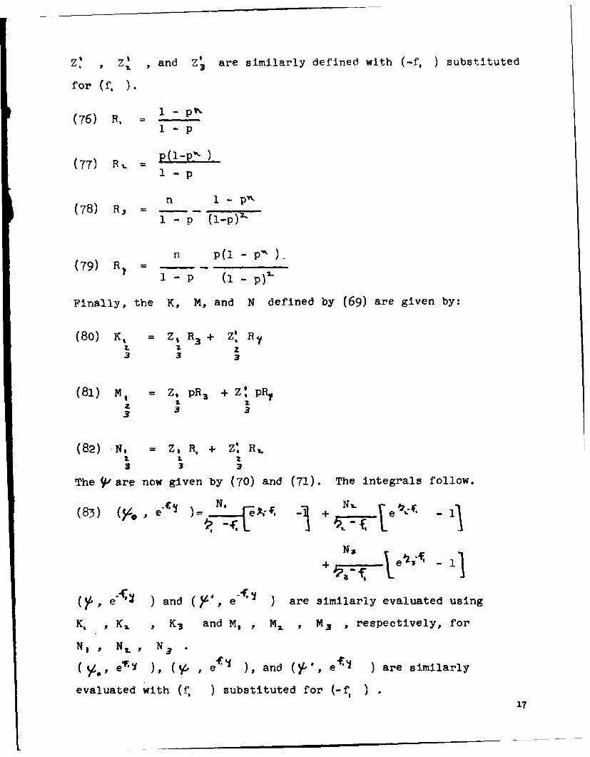
Z: z and z, are similarly defined with (-f, ) substituted

for (f, ).

1 - pV%(76) . - p

1-p

(77) RB. =1i-p

n p"(78) R, = - . ...

1 - p (1-p),

(79) R+ n- ~ W(9- p (1 -p)7

Finally, the K, M, and N defined by (69) are given by:

(80) K% = Z, R3 + Z: Ry2. % z3 3 3

(81) MI, = Z, pR3 + z: pRI

3 3 3

(82) N, = z, R, + z" R.2. 2 2

3 3 3

Thef? are now given by (70) and (71). The integrals follow.S•;N, Nz. e 92

(83) (Y-* , e"' ) 9r-, f + e- 4f-

+e

(,e., e' ) and (,', e-'f" ) are similarly evaluated using

K. , K1 , K3 and M, , M, , respectively, for

N, NL, N 3

(), ef ) and (,",ef'I ) are similarly

evaluated with (f, ) substituted for (-g )17

APPENDIX B

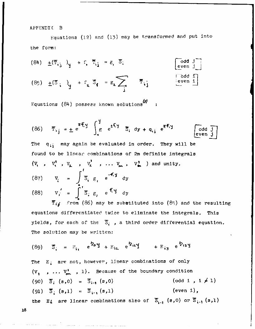
Eauations (!2) and (13) may be transformed and put into

the form:

(84) +Q(T ) + f' 7- g' odd Jf-Lven jJ

f bdd i(85) +(7 ) + ;S =g 7 even

Equations (84) possess known solutions

(86) T.j =+eg e d y + q; e een

The qai may again be evaluated in order. They will be

found to be linear combinations of 2m definite integrals

INv, , " v, v•,v" .. v,., V1 ) and unity.

(87) V. = J g, e dy

(88) V,- = e y

•Ir, from (86) may be substituted into (89) and the resulting

equations differentiated twice to eliminate the integrals. This

yields, for each of the S , a third order differential equation.

The solution may be written:

(89) 7. = e•"J + E; e';"'I + E 3 e 3'I

The E; are not, however, linear combinations of only

(VI , ... i., 1). Because of the boundary condition

(90) • (s,0) = S., (s,O) (odd i , i ý 1)

(91) •4 (s,l) = _,- (s,l) (even i),

the EZ are linear combinations also of •- (s,O) or r_• (s,l)

18

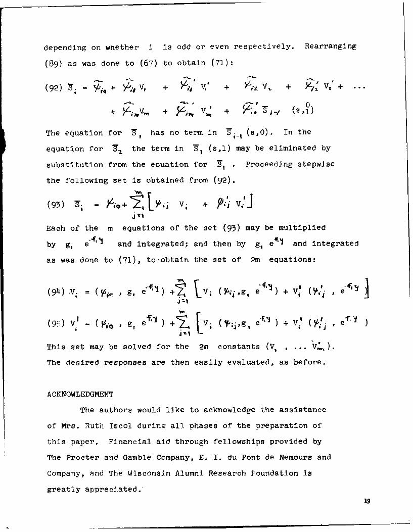
depending on whether i is odd or even respectively. Rearranging

(89) as was done to (67) to obtain (71):

(92) . : '/' + >L' V, + V*, V' + jPz V, + Y4Vz' +

+ + 3; + .. l,

The equation for • has no term in •- (s,O). In the

equation for 9. the term in -9 (s,l) may be eliminated by

substitution from the equation for 7 . Proceeding stepwise

the following set is obtained from (92).

(93) = o+j v1 + vie

Each of the m equations of the set (93) may be multiplied

by g, e"41 and integrated; and then by g, evI and integrated

as was done to (71), to-obtain the set of 2m equations:

(94) V. ( g,,. , G, ee) ($" g e + V ) + V: ( e

(9r-) V1 ;~. Y~'t. ge + [ U

This set may be solved for the 2m constants (V, , ... VA).

The desired responses are then easily evaluated, as before.

ACKNOWLEDGMENT

The authors would like to acknowledge the assistance

of Mrs. Ruth Iscol during all phases of the preparation of

this paper. Financial aid through fellowships provided by

The Procter and Gamble Company, E. I. du Pont de Nemours and

Company, and The Wisconsin Alumni Research Foundation is

greatly appreciated.

19

BIBLIOGRAPHY

1. "Transfer Function Analysis of Heat Exchangers," by

Y. Takahashi in Automatic and Manual Control, edited by

A. Tustin, Butterworth Scientific Publications, London,

1952, pp. 235 - 245.

2. "Regeltechnische Eigenschaften der Gleich - und Gegenstrom-

warmeaustauschern," by Y. Takahashi, Regelungstechnik,

Vol. 1, 2, 1953, PP. 32 - 35.

3. "Dynamic Characteristics of Double - Pipe Heat Exchangers,"

by W. C. Cohen and E. F. Johnson, Industrial and Engineering

Chemistry, Vol. 48, 6, 1956, pp. 1031 - 1034.

4. "Mean Temperature Difference in Design," by R. A. Bowman,

A. C. Mueller, and W. M. Nagle, Transactions of the ASME,

Vol. 62, 5, 1940, pp. 283 - 294.

5. "Advanced Mathematics for Engineers," by H. W. Reddick and

F. H. Miller, John Wiley and Sons, New York, Second

Edition, 1947, PP. 12 - 13.

6. "Methods of Applied Mathematics," by F. B. Hildebrand,

Prentice - Hall, Englewood Cliffs, N. J., 1952, pp. 385 - 386.

7. "College Algebra," by P. R. Rider, Macmillan, New York,

1940, pp. 203 - 205.

20