Comments on the Sachdev-Ye-Kitaev model

Juan Maldacena and Douglas Stanford

Institute for Advanced Study, Princeton, NJ 08540, USA

Abstract

We study a quantum mechanical model proposed by Sachdev, Ye and Kitaev. Themodel consists of N Majorana fermions with random interactions of a few fermionsat a time. It it tractable in the large N limit, where the classical variable is a bilocalfermion bilinear. The model becomes strongly interacting at low energies where itdevelops an emergent conformal symmetry. We study two and four point functionsof the fundamental fermions. This provides the spectrum of physical excitations forthe bilocal field.

The emergent conformal symmetry is a reparametrization symmetry, which isspontaneously broken to SL(2, R), leading to zero modes. These zero modes arelifted by a small residual explicit breaking, which produces an enhanced contributionto the four point function. This contribution displays a maximal Lyapunov expo-nent in the chaos region (out of time ordered correlator). We expect these featuresto be universal properties of large N quantum mechanics systems with emergentreparametrization symmetry.

This article is largely based on talks given by Kitaev [1], which motivated us towork out the details of the ideas described there.

arX

iv:1

604.

0781

8v1

[he

p-th

] 2

6 A

pr 2

016

Contents

1 Introduction 21.1 Organization of the paper and summary of results . . . . . . . . . . . . . . 4

2 Two point functions 82.1 The model . . . . . . . . . . . . . . . . . . . . . . . . . . . . . . . . . . . . 82.2 Summing the leading order diagrams . . . . . . . . . . . . . . . . . . . . . 82.3 The conformal limit . . . . . . . . . . . . . . . . . . . . . . . . . . . . . . . 102.4 Large q limit . . . . . . . . . . . . . . . . . . . . . . . . . . . . . . . . . . . 112.5 q = 2 . . . . . . . . . . . . . . . . . . . . . . . . . . . . . . . . . . . . . . 122.6 Computing the entropy . . . . . . . . . . . . . . . . . . . . . . . . . . . . . 132.7 Correction to the conformal propagator . . . . . . . . . . . . . . . . . . . 15

3 Four point functions 153.1 The ladder diagrams . . . . . . . . . . . . . . . . . . . . . . . . . . . . . . 163.2 Using conformal symmetry . . . . . . . . . . . . . . . . . . . . . . . . . . . 17

3.2.1 The four point function as a function of the cross ratio . . . . . . . 193.2.2 Eigenfunctions of the casimir . . . . . . . . . . . . . . . . . . . . . 203.2.3 The eigenvalues of the kernel kc(h) . . . . . . . . . . . . . . . . . . 223.2.4 The inner products 〈Ψh,Ψh〉 and 〈Ψh,F0〉 . . . . . . . . . . . . . . 233.2.5 The sum of all ladders . . . . . . . . . . . . . . . . . . . . . . . . . 253.2.6 Operators of the model . . . . . . . . . . . . . . . . . . . . . . . . . 263.2.7 Analytic continuation to the chaos region . . . . . . . . . . . . . . . 28

3.3 Proper treatment of the h = 2 subspace . . . . . . . . . . . . . . . . . . . . 303.3.1 The h = 2 eigenfunctions and reparameterizations . . . . . . . . . . 313.3.2 The shift in the eigenvalues . . . . . . . . . . . . . . . . . . . . . . 323.3.3 The enhanced h = 2 contribution . . . . . . . . . . . . . . . . . . . 353.3.4 Other terms from the h = 2 subspace . . . . . . . . . . . . . . . . . 38

3.4 More detail on the q =∞ four point function . . . . . . . . . . . . . . . . 393.5 Summary of the four point function . . . . . . . . . . . . . . . . . . . . . . 413.6 The chaos exponent at finite coupling . . . . . . . . . . . . . . . . . . . . . 42

3.6.1 The retarded kernel . . . . . . . . . . . . . . . . . . . . . . . . . . . 423.6.2 Large q . . . . . . . . . . . . . . . . . . . . . . . . . . . . . . . . . 433.6.3 General q . . . . . . . . . . . . . . . . . . . . . . . . . . . . . . . . 43

4 The effective theory of reparameterizations 45

5 The density of states and the free energy 49

6 Towards a bulk interpretation 516.1 Comments on kinematic space. . . . . . . . . . . . . . . . . . . . . . . . . 536.2 The fermions . . . . . . . . . . . . . . . . . . . . . . . . . . . . . . . . . . 54

1

6.3 Scrambling for near extremal black holes and its stringy corrections . . . . 55

7 Brief Conclusions 57

A The Schwinger-Dyson equations and the kernel 58

B The kernel as a function of cross ratios 59

C Representing F0 in terms of Ψh 60

D Writing Ψh(χ) in terms of Ψh,n(θ1, θ2) 60

E Direct approach to the shift in eigenvalue 61

F The first order change in h = 2 eigenvectors 63

G Numerical solution of the SD equations 65

H A model without the reparametrization symmetry 67

I Further coments on Kinematic space 70I.0.1 The kinematic space in the full model at q =∞ . . . . . . . . . . . 71

1 Introduction

Studies of holography have been hampered by the lack of a simple solvable model that cancapture features of Einstein gravity. The simplest model, which is a single matrix quantummechanics, does not appear to lead to black holes [2] (see [3] for a review). N = 4 superYang Mills at strong ’t Hooft coupling certainly leads to black holes, and exact results areknown at large N for many anomalous dimensions and some vacuum correlation functions,but at finite temperature the theory is difficult to study.

A system that reproduces some of the dynamics of black holes should be interacting,but we might hope for a model with interactions that are simple enough that it is stillreasonable solvable.

Kitaev has proposed to study a quantum mechanical model of N Majorana fermionsinteracting with random interactions [1]. It is a simple variant of a model introducedby Sachdev and Ye [4], which was first discussed in relation to holography in [5]. TheHamiltonian of [1] is simply

H =∑iklm

jiklmψiψkψlψm (1.1)

where the couplings jiklm are taken randomly from a Gaussian distribution with zero meanand a width of order J /N3/2.

2

One interesting feature of this model is that it develops an approximate conformalsymmetry in the infrared. Understanding how to deal with quantum mechanical theoriesthat develop such a conformal symmetry seems very important for both condensed matterphysics and gravity. One naively expects a full Virasoro symmetry. However, in themodel, the symmetry is both explicitly as well as spontaneously broken, so we end up with“nearly conformal quantum mechanics,” or NCFT1. (We propose to use the term NCFT1

to denote systems that have one time dimension which are nearly invariant under a fullreparametrization (or Virasoro) symmetry 1.) The same situation arises in gravity, whenwe consider very near extremal black holes. These are black holes that develop a nearlyAdS2 region, which we can call NAdS2, see [7] for a recent discussion. It is well known thatpurely AdS2 gravity is not consistent, except for the ground states. So the right setting inwhich to study holography for near extremal black holes is NAdS2/NCFT1.

Besides this structural similarity, it was noted in [8, 1] that the out of time ordercorrelators of the Sachdev-Ye-Kitaev model (1.1) (SYK) grow in a manner that reflectsan underlying chaotic dynamics. At relatively low energies this growth matches the oneexpected in a theory of gravity [9, 10, 11], which saturates the chaos bound [12].

In this paper we study this model a bit further. We start by summarizing the com-putation of the two point functions [4, 13] in the large N limit, following Sachdev, Ye,Parcollet, and Georges. We will discuss this in a variant of the model where the interac-tion involves q fermions at a time [1]. We will further show that the equations simplifyconsiderably in the large q limit. This allows us to connect analytically the free UV theoryto the interacting and nearly conformal IR theory. Further recent work in this or similarmodels includes [14, 15, 16, 17, 7, 18, 19]. See also [20, 21] for a string motivated modelwith disorder.

We then derive an explicit integral expression for the four point function in the infraredlimit. This problem was also considered in [19]. The four point function is actuallyinfinite in the strict conformal limit, due to Nambu-Goldstone bosons associated to thespontaneously broken reparameterization invariance. To remove the infinity we have totake into account the explicit breaking of this symmetry, which lifts these modes by a smallamount. We expect that this should be a universal feature of large, but finite, entropyNCFT1 systems. Namely, the systems cannot realize the conformal symmetry exactly2,and that the small explicit breaking leads to a universal contribution that dominates thefour point function and saturates the chaos bound.3 In particular, AdS2 dilaton gravity

1This should be contrasted to what is usually called “conformal quantum mechanics”, such as [6], whichare only invariant under SL(2, R).

2The argument in [22] shows that an exact SL(2, R) symmetry is incompatible with a thermofieldinterpretation with a finite number of states. Of course, in gravity the exact SL(2, R) symmetry is brokenby the presence of a dilaton field, see [7] for recent discussion.

3In 1 +1 dimensional CFT the conformal symmetry is also spontaneously broken (recall that L−2|0〉 6=0), but it is not explicitly broken. In that case we also have a universal (stress tensor) contribution to thefour point function. By itself this piece saturates the chaos bound [23, 24, 25], but only in special theoriesdoes it dominate.

3

is an example with the same explicit breaking [26], leading to the same dominant term inthe four point function.

In addition to this term, the SYK four point function contains subleading pieces thatare finite in the low temperature limit. These contain information about the compositeoperators that appear in the operator product expansion of

∑i ψi(τ)ψi(0). These get

anomalous dimensions at leading order in N and seem analogous to the single trace oper-ators of the usual gauge theory examples of holography. One finds a tower of states withan approximately integer spacing. This tower of states is reminiscent of the one appearingin large N O(N) models, where we have one state for each spin. Here we get a similarstructure, but with dimensions which have O(1) corrections relative to the dimensions inthe free theory. This suggests that the bulk theory contains low-tension strings. Theseextra states do not compete with the dilaton gravity piece, even though the strings arelight, simply because of the enhancement of gravity in NAdS2.

Much of the analysis in this paper, including the ladder diagrams, the spectrum ofthe kernel kc(h), and the effective theory of reparameterizations, is simply what Kitaevpresented in his talks [1], and we are thankful to him for several further explanations.

1.1 Organization of the paper and summary of results

The article might seem a bit technical in some parts, so we will summarize below whatis done in various sections. The reader might want to jump directly the the sections thatlook most interesting to him/her.

In section two we review the large N structure of the theory. The model has onedimensionful parameter J , with dimensions of energy, which characterizes the size of theinteraction terms in the Hamiltonian. This implies that the interaction is relevant andbecomes strong at low energies. For large N the diagrams have a simple structure that isreminiscent of the one for large N O(N) theories (see also the discussion in [18]). There is abilocal field G(τ1, τ2) depending on two times which becomes classical in the large N limit.On the classical solution, G, this field is equal to the two point function of the fermionsG(τ1, τ2) = 1

N

∑Ni=1〈ψi(τ1)ψi(τ2)〉. The classical equation for G is non-local in time but

it can be solved numerically. G can be inserted in the action to compute the partitionfunction. We also show that in the variant of the model where q fermions interact at atime, then the large q limit becomes analytically tractable and one can solve the classicalequations for any value of the coupling. Another simple solvable limit is the case q = 2.In that case, the Hamiltonian has the form H = i

∑kl jklψkψl which is a random mass-

like term. This can be diagonalized and we get a spectrum of masses, or energies, givenby the usual semi-circle law distribution for random matrices. This particular exampleis integrable and some properties are different than the one for the generic q case. Inparticular, we find that there is no exponentially growing contribution to the out of timeorder four point function.

At low energies the model simplifies further due to the emergence of a conformal sym-metry. In one dimension the conformal group is the same as the group of all reparame-

4

terizations. One can see this symmetry explicitly in both the low energy action, or thelow energy equations for the bilocal fields. One might expect a theory that has a fullreparameterization symmetry to be topological. This is not the case here because thereparameterization symmetry is spontaneously broken down to an SL(2, R) subgroup. Inother words, the bilocal function G(τ1, τ2) = G(τ1 − τ2) becomes Gc ∝ τ−2∆

12 for largevalues of J τ12 (with τ12 = τ1 − τ2). The partition function displays a zero temperatureentropy of order N . In addition, there is a finite temperature entropy which is linear inthe temperature, proportional to N/(βJ ). Generically the model is expected to have asingle ground state, but here we are considering temperatures that are fixed in the largeN limit. This means that we are accessing an exponentially large number of states.

In section three we discuss general features of the four point function of the fermions〈ψiψiψjψj〉. This can also be viewed as a two point function of the bilocal fields. The finalform for the leading 1/N piece in for the four point function is displayed in (3.149).

This computation of the four point function is a bit technical and, for this reason, thissection is rather long. The diagrams that contribute have the form of ladder diagrams.Therefore, they can be summed by defining a kernel K that corresponds to adding arung to a ladder. Then the full ladder has a form proportional to 1

1−KF0 where F0 isa diagram with no rungs. This is conceptually easy. However, it is tricky to invert thekernel since one has to understand in more detail the space of functions where it is acting.Fortunately the problem partially simplifies at low energies due to the unbroken SL(2, R)symmetry. This symmetry can be used to diagonalize the kernel and also to describe thespace of functions we should sum over. This leads to a relatively explicit expression forthe four point function in terms of a sum over intermediate states (3.88), (3.90), once weexclude the Goldstone bosons which need to be treated separately. We can read off thespectrum of operators that appear in the OPE expansion of two fermions.The spectrumis given by the solutions hm to the equation kc(hm) = 1, with kc(h) in (3.73). We canvaguely view this tower of operators as ψi∂

1+2mψi. We say “vaguely” because the properdimensions we obtain from the above procedure display an order one correction from thenaively expected values (which would be 2∆ + 1 + 2m). This is an important clue for apossible bulk interpretation. It is saying that the fermions cannot be associated to weaklyinteracting particles in the bulk. Their interactions would have to be of order 1 ratherthan 1/N .

We then give a proper treatment for the Goldstone modes that have Kc = 1 in theconformal limit. These arise from reparametrizations of the conformal solution, Gc. Thesefluctuations have zero action in the conformal limit, but get a non-zero action when wetake into account the leading corrections to the conformal answers. We first take a directapproach and compute the leading correction to the classical solution G away from theconformal limit G = Gc + δG. It turns out that the leading correction involves an extrafactor of 1/J . One can then proceed to compute the variation of the kernel K away fromthe conformal limit K = Kc + δK. We then evaluate δK on reparametrizations of theconformal solution δεGc, where ε(τ) is an infinitesimal reparametrization. We get a non-zero answer which can then be used to compute the four point function. Since δK ends

5

up in the denominator in the expression for the four point function, we get an enhancedcontribution with an additional factor of (βJ ) as compared to the conformal answer,which is independent of βJ . This enhanced contribution is not conformally covariant.However, it has a very simple form in the OPE limit which can be understood as follows.The OPE gives rise to an energy operator of the model, which has quadratic fluctuations〈(δE)2〉 in the thermal ensemble. These fluctuations are governed by the specific heat ofthe system, which again is non-zero once we take into account the effects of the breakingof the conformal symmetry. We also consider the contribution of these Goldstone modes

in the chaos limit. There they give the dominant term (βJ /N)e2πβt that saturates the

bound. The reparametrization symmetry of the model is essential to obtain this PseudoGoldstone boson. In appendix H we discuss a model that has a low energy SL(2, R)symmetry but without the conformal symmetry, by thinking of the couplings as dynamicalwith an SL(2, R) invariant correlation function. In this case there is no Pseudo-Goldstonemode, the low energy physics is SL(2, R) invariant and the chaos exponent is less thanmaximal.

In section four, we give a discussion of the four point function from the perspectiveof the large N effective action for the bilocal field G, see also [18]. The intermediate statesthat appear can be understood from the on-shell condition for fluctuations of this field.The enhanced non-conformal part of the four point function arises from the functionalintegral over G configurations that are reparameterizations of the infrared saddle pointsolution. We give a simple effective field theory argument showing that the effectiveaction is given by the Schwarzian derivative, f(τ), τ, of the reparametrization (4.176),with a coefficient of order (βJ )−1 [1]. This action constitutes an explicit breaking of theconformal symmetry. It can be used to derive the enhanced contribution mentioned above,and also to compute the specific heat.

In section five we discuss some features of the spectrum of the model. We startby presenting a numerical computation of the spectrum for the case of N = 32. Thespectrum in this case looks reminiscent to that of a random matrix and, as expected, isstatistically symmetric under H → −H since the random couplings can be positive as wellas negative. At low temperature one is interested in the region near the bottom end ofthe spectral distribution. We then look at the expression for the free energy at leadingorder in N , which has the low-temperature expansion logZ = −βE0 + S0 + c

2βwhere all

terms are of order N . The first term is the ground state energy, which is not interesting.The second is the zero temperature entropy. The third, with the specific heat c ∝ N/J ,arises from the breaking of the conformal symmetry and can be computed in terms ofthe Schwarzian action for the reparametrizations, after noticing that we can change thetemperature by making a reparametrization of the Euclidean circle (or, equivalently, wecan go from the circle to the line by a reparametrization). We further consider the N0

correction to logZ. This arises from the one loop correction to the effective action forthe bilocal fields. All the modes that have a non-vanishing action give a contributionjust to E0 and S0, since they are J independent (up to UV contributions to E0). Thereparametrization modes give a term that contributes a logarithm to the free energy [27],

6

specifically −32

log(βJ ). This additional contribution has an interesting effect. It impliesthat if we compute the spectral density ρ(E) by inverse Laplace transforming Z(β) we

obtain that ρ(E) ∝ J −1eS0+√

2c(E−E0), with no prefactor powers of (E − E0), in theregime where we can trust the computation.

In section six we comment on the possible bulk interpretation. The enhanced non-conformal contribution agrees with the four point function one expects in a theory ofdilaton gravity [28, 26]. This contribution is completely general in any situation witha near extremal black hole with a NAdS2 region and it follows by the same pattern ofspontaneous plus explicit breaking of the conformal symmetry [26] (see [25] for a similardiscussion in the AdS3/CFT2 context). Therefore the information about other possiblebulk states comes from the contribution that is J independent and finite in the conformallimit. These are the states that appeared in the OPE expansion of two fermions. Thislooks like a single Regge trajectory with dimensions that are linearly increasing with “spin”,though spin is hard to define in two dimensions. This implies that a dual description wouldinvolve a string with low tension, with ls ∼ RAdS.

Part of our motivation to study this model arose from the observation that the fourpoint function was saturating the chaos bound, which is a necessary condition for a gravitydual. It was shown in [11] that stringy corrections to the chaos exponent involve a factorof 1− l2s/R2 where R is a suitable distance scale. This suggested that the condition mightalso be sufficient to exclude models with light strings. However, examining the scale Rcarefully, it is possible to show that for near extremal black holes this correction has the

form(

1− l2sR2AdS

(S−S0)S0

), where S is the entropy and S0 is the zero temperature entropy.

Since the ratio of entropies is much less than one, we see that stringy corrections to theLyapunov exponent are very suppressed, suggesting that even in cases with ls ∼ RAdS2 wecould have a Lyapunov exponent close to the gravity value. In other words, for this casea nearly saturated Lyapunov exponent is not a guarantee of a high string tension. Andindeed, in the SYK model we seem to have a low string tension. A related perspective onthis is the following: the four point function saturates the bound because it is dominatedby the universal “gravity” piece coming from the zero modes discussed above. This turnsout to be enhanced by a factor of S0/(S − S0). Relative to this piece, the “stringy”contributions to the four point function are small, so they have only a mild effect on thechaos exponent.

We also comment on the bulk interpretation of the fermion fields. We speculate thatwe should not have N fermions in the bulk, but rather one fermion with a string attachedto the boundary.

Finally, we note that the bilocal field can be viewed as a field in one more dimension.At low energies the extra dimension defined in this way has a metric characterized by theconformal group and can be viewed as a dS2 (or AdS2) space in accordance with recentdiscussions of kinematic space [29, 30]. This follows simply from the structure of theconformal group. Some terms in the action can be viewed as local terms in this space, butothers have a non-local expression.

7

In the appendices we give some more details on the computations.

2 Two point functions

2.1 The model

We consider a quantum mechanical model with N Majorana fermions with random interac-tions involving q of these fermions at a time, where q is an even number. The Hamiltonianis

H = (i)q2

∑1≤i1<i2<···<iq≤N

ji1i2···iqψi1ψi2 · · ·ψiq (2.2)

〈j2i1···iq〉 =

J2(q−1)!

N q−1=

2q−1

q

J 2(q−1)!

N q−1(no sum) (2.3)

We take each coefficient to be a real variable drawn from a random gaussian distribution.(2.3) indicates the variance of the distribution. It is characterized by a dimension oneparameter J , (or J , which is defined with an extra factor that makes the model moreuniform in q) which we take to be the same for all coefficients. The numerical factors, andfactors of N , are introduced to simplify the large N limit. A factor of i is necessary tomake the Hamiltonian Hermitian when q = 2 mod(4). This i means that the system isnot time reversal symmetric for odd q/2. Thus, if we restrict to time reversal symmetricinteractions the model with q = 4 represents the dominant interactions at low energy.The others involve some degree of tuning. We assume that the system does not have aspin glass transition [31] and we work to leading order in the 1/N expansion. Thoughthe model generically has a unique ground state, we work at temperatures which are fixedin the large N expansion, implying that we access an exponentially large number of lowenergy states, of order O(eαN), α > 0.

2.2 Summing the leading order diagrams

We will work first in Euclidean space. It is useful to define the Euclidean propagator as

G(τ) ≡ 〈T (ψ(τ)ψ(0))〉 = 〈ψ(τ)ψ(0)〉θ(τ)− 〈ψ(0)ψ(τ)〉θ(−τ) (2.4)

For a free Majorana fermion this is very simple

Gfree(τ) =1

2sgn(τ) , Gfree(ω) = − 1

iω=

∫dteiωτGfree(τ) (2.5)

Gfree has the same expression at finite temperature, with τ ∼ τ + β. Notice that it iscorrectly antiperiodic as τ → τ + β. . These equations also normalize the fermion fieldsappearing in the interaction (2.2). Recall that the free Majorana fermions are simplydescribed by operators that are essentially N dimensional Dirac γ matrices, see e.g. [17].

8

Using this free propagator we can then compute corrections due to the interaction. Letus look at the first correction to the two point function, shown in figure 1. This arisesby bringing down two insertions of the interaction Hamiltonian and then averaging withrespect to the disorder. The disorder average is represented by a dotted line in figure 1. Aspointed out in [19], we can sometimes reproduce similar diagrams by considering ji1,··· ,iq tobe a dynamical field. Here we will stick to the disordered model. The disorder average linksthe indices appearing in the two interaction Hamiltonians and we end up with a correctionthat scales as J2 relative to the free two point function, with no additional factors of N ,since we get (q − 1) factors of N from the sum over the indices of the intermediate lines.

+ + + +

Figure 1: Diagrams representing corrections to the two point function, for the q = 4 case.The free two point function is given by the straight line. The first correction involves alsoan average over disorder, which is represented by a dashed line. We have also indicated acouple more diagrams that also contribute at leading order in N .

= + + +

=

Figure 2: Equations that define the summation of the leading large N contributions, forthe q = 4 case. The solid circle represents the one particle irreducible contributions. Thedotted circle represents the full two point function. This is a graphical representation ofthe equations in (2.6).

Besides this first diagram, there are many more “iterated watermelon” diagrams thatcontribute at leading order in N . Two more are shown in figure 1. The set of diagramsis sufficiently simple that they can be summed by writing self consistency equations forthe sum. First, it is convenient to define a self energy, Σ(τ, τ ′), which includes all the oneparticle irreducible contributions to the propagator. By translation symmetry, Σ(τ, τ ′) =

9

Σ(τ − τ ′) and we can write the full two point function, and the definition of Σ as

1

G(ω)= −iω − Σ(ω) , Σ(τ) = J2 [G(τ)]q−1 (2.6)

Notice that the first equation is written in frequency space while the second in the original(Euclidean) time coordinate. Here we have assumed translation symmetry. The possiblevalues of the frequency depend on whether we are at β = ∞, where it is continuous, orat finite β where we have ω = 2π

β(n + 1

2). When we talk about zero temperature, we are

imagining taking the large N limit first and then the zero temperature limit.As a side comment, note that we could consider a model with a Hamiltonian which is

a sum of terms with various q’s, and with random couplings with their own variance Jq.The large N equations for such models would be very similar except that the right handside of (2.6) would be replaced by Σ =

∑q J

2q [G(τ)]q−1. But we did not find any good use

for this.

2.3 The conformal limit

At strong coupling, the first equation in (2.6) can be approximated by ignoring the firstterm on the right hand side. It is convenient to write these approximate equations as∫

dτ ′G(τ, τ ′)Σ(τ ′, τ ′′) = −δ(τ − τ ′′) , Σ(τ, τ ′) = J2 [G(τ, τ ′)]q−1

(2.7)

Written in this form, they are invariant under reparametrizations,

G(τ, τ ′)→ [f ′(τ)f ′(τ ′)]∆G(f(τ), f(τ ′)) , Σ(τ, τ ′)→ [f ′(τ)f ′(τ ′)]

∆(q−1)Σ(f(τ), f(τ ′))

(2.8)provided that ∆ = 1/q.

We can then use an ansatz of the form

Gc(τ) =b

|τ |2∆sgn(τ), or Gc(τ) = b

[π

β sin πτβ

]2∆

sgn(τ) (2.9)

where we have given also the finite temperature version, which follows from (2.8) withf(τ) = tan τπ

β. We can determine b by inserting these expressions into the simplified

equations and obtain

J2bqπ =

(1

2−∆

)tanπ∆ , ∆ =

1

q(2.10)

We will use ∆ and 1/q interchangeably below. To derive the first equation here, it isconvenient to use the Fourier transform∫ ∞

−∞dτeiωτ

sgn(τ)

|τ |2∆= i 21−2∆

√π

Γ(1−∆)

Γ(12

+ ∆)|ω|2∆−1sgn(w) (2.11)

10

From (2.9) it is possible also to compute the Lorentzian time versions by setting τ = it.Since the correlator is not analytic at τ = 0 it is important to know whether we are doingthe analytic continuation of the τ > 0 or the τ < 0 Euclidean expressions. The twochoices give different choices of ordering of the Lorentzian correlator. For example, thecontinuation of the τ > 0 form of the Euclidean correlator gives

〈ψ(t)ψ(0)〉 = Gc,E(it+ ε) = be−iπ∆

(t− iε)2∆(2.12)

where we summarized the fact that we continue from τ > 0 by the t→ t− iε prescription.This equation is valid for any sign of t. Of course the other ordering can be obtainedby continuing from the τ < 0 version. We can also get the finite temperature version byreplacing (t− iε)→ β

πsinh [π(t− iε)/β] in (2.12).

It is sometimes also convenient to introduce the retarded propagator defined as

Gc,R(t) ≡ 〈ψ(t)ψ(0) + ψ(0)ψ(t)〉 θ(t) = 2b cos(π∆)

[π

β sinh πtβ

]2∆

θ(t) (2.13)

where θ(t) is the step function. Of course, (2.13) also shows that the dimension ∆ sets thequasinormal mode frequencies as ωn = −i2π

β(∆ + n).

Here we have given the conformal limit of the expressions. For large βJ , it is possible tosolve the equations (2.6) numerically to obtain expressions that smoothly interpolate be-tween the free UV limit and the infrared expressions given above, see figure 15 in appendixG. In addition, in the next subsection we show how to do this interpolation analyticallyin the large q limit.

2.4 Large q limit

One convenient feature of the model in (2.2) is the fact that it simplifies considerably forlarge q.4 We can write

G(τ) =1

2sgn(t)

[1 +

1

qg(τ) + · · ·

], Σ(τ) = J221−qsgn(τ)eg(τ)(1 + · · · ) (2.14)

where the dots involve higher order terms in the 1/q expansion. We will work in the regimewhere g(τ) is of order one. In this regime we can approximate

1

G(ω)=

1

− 1iω

+ [sgn×g](ω)2q

= −iω + ω2 [sgn× g](ω)

2q= −iω − Σ(ω) (2.15)

where in the first equality we fourier transformed the first equation in (2.14) and weexpanded in powers of 1/q in the second equality, keeping only the first nontrivial term.

4We are grateful to S.H. Shenker for discussions on this point.

11

Comparing this expression for Σ with the one in (2.14) we get the equation

∂2t [sgn(τ)g(τ)] = 2J 2sgn(τ)eg(τ) , J ≡ √q J

2q−1

2

(2.16)

This equation determines g(τ). It is well defined in the large q limit, when we scale J sothat J is kept fixed as q → ∞. Of course, since J is dimensionful, we can always go tosome value of τ where this equation will be valid. We are interested in a solution withg(τ = 0) = 0. In other words, at short distances we should recover the free fermion result.The derivation of this equation is valid both for zero temperature and finite temperature.The general solution is

eg(τ) =c2

J 2

1

sin(c(|τ |+ τ0))2(2.17)

We can now impose the boundary conditions g(0) = g(β) = 0 to obtain

eg(τ) =

cos πv2

cos[πv(1

2− |t|

β)]2

(2.18)

βJ =πv

cos πv2

. (2.19)

The second equation determines the parameter v, which ranges from zero to one as βJranges from zero to infinity. It is also possible to take the β = ∞ limit of the aboveexpressions to obtain

eg(τ) =1

(|t|J + 1)2 (2.20)

Note that these results imply that Σ changes more rapidly than G. In fact, G is almostconstant, and almost equal to 1

2sgn(τ), when Σ is changing to its IR value.

2.5 q = 2

Another solvable example is the case of q = 2. In this case we can solve (2.6) as

G(ω) = − 2

iω + i sgn(ω)√

4J2 + ω2(2.21)

This is the same as the one studied in [32, 33, 20]. For positive euclidean time we get

G(τ) = sgn(τ)

∫ π

0

dθ

πcos2 θe−2J |τ | sin θ (2.22)

=1

πJτ− 1

4π(Jτ)3+ · · · , Jτ 1 (2.23)

For this particular case, we can simply diagonalize the Hamiltonian (2.2), since it isquadratic. We get a set of fermionic oscillators with some masses. The masses have a

12

semicircle law distribution, since we are diagonalizing a random mass matrix. Near zerofrequencies the distribution is constant and we get the same as what we expect for a 1 + 1dimensional fermion field (from θ ∼ 0, π above). The spacing between the frequencies goeslike 1/N , so this fermion is on a large circle. In this sense this example is a bit trivial sinceit is the same as free fermions. However, it is useful to view it as an extreme example ofthe more interesting models with q > 2. Therefore, in this model we indeed get a fermionin an extra dimension. However, note that we get a single fermion, not N fermions in theextra dimension. We can also simply obtain the finite temperature expression for the twopoint function by summing over images in the zero temperature answer

Gβ(τ) =∞∑

m=−∞

Gβ=∞(τ + βm)(−1)m =

∫ π

0

dθ

πcos2 θ

cosh[( τβ− 1

2)2Jβ sin θ]

cosh(Jβ sin θ)(2.24)

2.6 Computing the entropy

It is possible to write the original partition function of the theory as a functional integralof the form [1, 14]

e−βF =

∫DGΣ exp

[N

log Pf(∂t − Σ)− 1

2

∫dτ1dτ2

[Σ(τ1, τ2)G(τ1, τ2)− J2

qG(τ1, τ2)q

]](2.25)

It can be checked that the classical equations obtained from this reproduce the equationsin (2.6), when we vary with respect to G and Σ independently. Here the tildes remind usthat we are are thinking about the integration variables, while G, Σ without tildes are thesolutions of the classical equations from (2.26), obeying (2.6). Substituting those solutionsinto (2.25) we get the leading large N approximation to the free energy:

−βF/N = log Pf(∂t − Σ)− 1

2

∫dτ1dτ2

[Σ(τ1, τ2)G(τ1, τ2)− J2

qG(τ1, τ2)q

](2.26)

In the q = ∞ model we know the full solutions for G and Σ, so we can insert themin (2.26) to obtain the free energy. In order to avoid evaluating the Pfaffian term, it isconvenient to take a derivative with respect to J∂J of the free energy (2.26). Due tothe fact that G and Σ obey the equations of motion, the only contributing term is thederivative of the explicit dependence on J , so that we obtain

J∂J(−βF/N) =J2β

q

∫ β

0

dτG(τ)q = −βq∂τG|τ→0+ = −βE (2.27)

where we have used the equations (2.6) in position space. Since the partition functiononly depends on the combination βJ , then J∂J is the same as β∂β. Therefore the aboveexpression gives us the energy.

As q →∞, we can insert the solution (2.18) into (2.27). We can also use the equation(2.16) to do the integral. Furthermore we can turn J∂J → J ∂J and use (2.19) to turn it

13

into a derivative with respect to v, always keeping q and β fixed. This gives

J ∂J (−βF/N) =v

1 + πv2

tan πv2

∂v(−βF/N) (2.28)

=β

4q2

∫ β

0

dτ2J 2eg(τ) =β

4q22(−g′(0)) =

πv

q2tan

πv

2(2.29)

−βF/N =1

2log 2 +

1

q2πv[tan(πv

2

)− πv

4

](2.30)

where we fixed the integration constant using that for J → 0 we should recover the freevalue, which is simply the log of the total dimension of the Hilbert space. The expansionaround weak coupling is simply an expansion in powers of v2, which translates into anexpansion in powers of (βJ )2, as expected. On the other hand, at strong coupling we canuse (2.19) to find

v = 1− 2

βJ+

4

(βJ )2− (24 + π2)

3(βJ )3+ · · · (2.31)

Then, the term of order 1/q2 in (2.30) behaves as

1

q2

[2

1− v− (2 +

π2

4) +

π2

3(1− v) + · · ·

]=

1

q2

[(βJ )− π2

4+

π2

2(βJ )+ · · ·

](2.32)

Here the first term can be interpreted as a correction to the ground state energy. Thesecond term is a correction to the zero temperature entropy, to which the 1

2log 2 term in

(2.30) also contributes. Finally the third term is a temperature dependent correction tothe entropy, or near extremal entropy, which goes like T for low temperature.

The temperature independent piece can be compared with the result obtained in [1]for general q (see the earlier [31] for the q = 4 case using the Sachdev-Ye model)

S0

N=

1

2log 2−

∫ ∆

0

dxπ(1

2− x) tanπx ∼ 1

2log 2− π2

4q2+ · · · (2.33)

where the last expression is the approximate answer for large q, which agrees with thetemperature independent pice of (2.30) using (2.32).

It is also possible to compute the free energy at q = 2. Directly from the free fermionpicture, and subtracting the ground state energy, we find

logZ/N =

∫ π

0

dθ

πcos2 θ log

[1 + e−2Jβ sin θ

]∼ π

12βJ+ · · · , for βJ 1 (2.34)

We see that at small temperatures the entropy vanishes, in agreement with the first equalityin (2.33) with ∆ → 1

2. We can also see that for large temperatures this reproduces the

value S/N = 12

log 2.

14

We will later show that for general q the expression of the free energy has the form

logZ = −βE0 + S0 +c

2β(2.35)

plus higher orders in 1/β. Here E0 is the ground state energy, S0 is the zero temperatureentropy and c/β is the specific heat. E0, S0 and c are all of order N . The exact largeN free energy can be computed numerically for general q. Appendix G contains somediscussion of this.

2.7 Correction to the conformal propagator

It is also interesting to consider the leading correction to the conformal two point function.For large q the conformal answer is

Gc =b sgn(τ)

|τ |2q

=1

2

1

|J τ |2∆, J 2(2b)q = 1 (2.36)

Using (2.14) and (2.20), we find the leading correction

G(τ) = Gc(τ)

(1− 2

q

1

J |τ |+ · · ·

). (2.37)

At finite temperature, we use (2.18) to find

G(τ) = Gc(τ)

[1− 2

q

1

βJ

(2 +

π − 2π|τ |/βtan π|τ |

β

)+ · · ·

]. (2.38)

On the other hand, for q = 2 we see from (2.23) that the order 1/J correction vanishes.We will later discuss general values of q.

3 Four point functions

In this section, we analyze the leading 1/N piece of the four point function, at strongcoupling βJ 1. In any correlation function, the average over disorder ji1,...,iq will givezero unless the indices of the fermions are equal in pairs. This means that the most generalnonzero four point function is

〈ψi(τ1)ψi(τ2)ψj(τ3)ψj(τ4)〉. (3.39)

We will consider the case in which we average over i, j. (The pure i = j and i 6= j casesare related in a simple way.) The averaged correlator

1

N2

N∑i,j=1

〈T (ψi(τ1)ψi(τ2)ψj(τ3)ψj(τ4))〉 = G(τ12)G(τ34) +1

NF(τ1, ..., τ4) + · · · (3.40)

has a disconnected piece given by a contraction with the dressed propagators, plus a powerseries in 1/N . We will analyze the first term in this series, F .

15

+ + + +τ1

τ2

τ3

τ4

Figure 3: Diagrams representing the 1/N term in the index-averaged four point function,for the q = 4 case. One should also include the diagrams with (τ3 ↔ τ4) and a relativeminus sign. The propagators here are the dressed two point functions discussed above.

=

Figure 4: The (n+1)-rung ladder Fn+1 can be generated from the n-rung ladder by “mul-tiplication” with the kernel K, shown in blue. We call the vertical propagators a “rung”and the horizontal ones a “rail”.

3.1 The ladder diagrams

The diagrams that one must sum to compute F are ladder diagrams with any number ofrungs, built from the dressed propagators discussed in the previous section. The first fewdiagrams for F are shown in figure 3. We will use Fn to denote the ladder with n rungs,so that F =

∑nFn. The first diagram, F0, is just a product of propagators

F0(τ1...τ4) = −G(τ13)G(τ24) +G(τ14)G(τ23). (3.41)

This piece contributes at order 1/N because the propagators set i = j in the sum of (3.40).The next diagram is a one-rung ladder, where we integrate over the locations of the endsof the rung:

F1 = J2(q − 1)

∫dτdτ ′

[G(τ1 − τ)G(τ2−τ ′)G(τ−τ ′)q−2G(τ−τ3)G(τ ′−τ4)− (τ3 ↔ τ4)

].

(3.42)In this expression, the factor of (q− 1) comes from the choice of which of the lines comingout of the interaction vertex should be contracted into a rung, and which should continueon as the side rail. This diagram also contributes at order 1/N , because the 1/N q−1 scalingof the product of two couplings multiplies a factor of N q−2 from the sum over (q−2) indicesin the rung loops. One can check that all of the ladder diagrams (and only these!) areproportional to 1/N .

The standard technique for summing a set of ladder diagrams is to use the fact that theyare generated by multiplication by a kernel K. This is illustrated in figure 4. Explicitly,

Fn+1(τ1, τ2, τ3, τ4) =

∫dτdτ ′K(τ1, τ2; τ, τ ′)Fn(τ, τ ′, τ3, τ4), (3.43)

where the kernel is

K(τ1, τ2; τ3, τ4) ≡ −J2(q − 1)G(τ13)G(τ24)G(τ34)q−2. (3.44)

16

It is convenient to think about the integral transform in (3.43) as a matrix multiplication,where the first two arguments of K form one index of the matrix, and the last two formthe other index. The sum of all ladder diagrams is then a geometric series that can besummed by matrix inversion:

F =∞∑n=0

Fn =∞∑n=0

KnF0 =1

1−KF0. (3.45)

To carry this out, we would like to understand how to diagonalize K. The way we havedefined it, K is not a symmetric operator under (τ1, τ2) ↔ (τ3, τ4). However, we canconjugate by a power of the propagator to get a symmetric version

K(τ1, τ2; τ3, τ4) ≡ |G(τ12)|q−2

2 K(τ1, τ2; τ3, τ4)|G(τ34)|2−q

2 (3.46)

= −J2(q − 1)|G(τ12)|q−2

2 G(τ13)G(τ24)|G(τ34)|q−2

2 . (3.47)

This is enough to show that K has a complete set of eigenvectors. We will consider thiskernel as acting on the space of anti-symmetric functions of two arguments, say τ3, τ4. Wewill use both K and K in what follows.

3.2 Using conformal symmetry

So far, what we have said is true for any value of the coupling βJ . In order to proceedfurther, we will go to the conformal limit βJ 1. In this limit we can use the conformalexpressions for Gc(τ) (2.9). It is worth noting that the J dependence in K drops out in theconformal limit. This is due to the factors of b in the infrared expressions for G (2.9) and(2.10). In the conformal limit computations on the zero temperature line are equivalentto computations on the finite temperature circle, after using the map

τline = f(τcircle) = tanπτcircleβ

. (3.48)

This is a special case of the general reparametrization symmetry (2.8). The expressionsfor the propagators are simpler when we consider the theory on the line, so we will workthere for most of this section. Substituting (2.9) into the kernel we get

Kc(τ1, τ2; τ3, τ4) = − 1

α0

sgn(τ13)sgn(τ24)

|τ13|2∆|τ24|2∆|τ34|2−4∆(3.49)

α0 ≡2πq

(q − 1)(q − 2) tan πq

=1

(q − 1)J2bq. (3.50)

It will turn out that we can safely compute some, but not all, of the large-βJ correlatorusing this expression for K. The reason is that some of the eigenfunctions have eigenvalueKc = 1 in the conformal limit, leading to a divergence in the geometric series (3.45). When

17

the time comes, in section 3.3, we will treat those eigenfunctions in perturbation theoryoutside the conformal limit. For now, we proceed with (3.49).

The key property that makes it possible to diagonalize (3.49) is conformal invariance.This can be presented using the following generators of an SL(2) algebra

D = −τ∂τ −∆, P = ∂τ , K = τ 2∂τ + 2τ∆

[D, P ] = P, [D, K] = −K, [P , K] = −2D. (3.51)

Here ∆ = 1/q is the conformal dimension of the fermion. These generators commute withthe kernel Kc, in the sense that up to total derivatives with respect to τ3 and τ4, we have

(D1 + D2)Kc(τ1, τ2; τ3, τ4) = Kc(τ1, τ2; τ3, τ4)(D3 + D4) (3.52)

and similarly for the P and K generators. (These are the generators appropriate for actingon the non-symmetric kernel Kc. To get a set that commutes with the symmetric versionKc we should replace ∆ by 1/2.)

This symmetry is useful in two ways. First, it implies that the ladder diagrams Fn aresimple powers times a function of the SL(2) invariant cross ratio:

χ =τ12τ34

τ13τ24

. (3.53)

This is because the function F0 in (3.41) transforms like a conformal four point function,and this property is preserved by acting with an SL(2) invariant operator. This will allowus to represent the kernel in the space of functions of a single cross ratio, rather than inthe space of functions of two times. In other words, we can consider Kc(χ; χ) instead ofKc(τ1, τ2; τ3, τ4). Second, it implies that the kernel commutes with the casimir operatorC1+2 built from the sum of the generators acting on the two times:

C1+2 = (D1 + D2)2 − 1

2(K1 + K2)(P1 + P2)− 1

2(P1 + P2)(K1 + K2)

= 2(∆2 −∆)− K1P2 − P1K2 + 2D1D2. (3.54)

The casimir is a differential operator with a family of eigenfunctions given by simple powerstimes functions Ψh(χ). Because the spectrum is nondegenerate, these must be exactly theeigenfunctions of the kernel Kc(χ; χ) acting in the space of cross ratios. This leads to arecipe for the four point function:

1. Understand the properties of F and Fn as functions of the cross ratio.

2. Find the eigenfunctions of C1+2 with these properties. These are particular hyper-geometric functions Ψh(χ), related to conformal blocks of weight h.

3. Determine the set of h to have a complete basis of functions. This turns out to beh = 1

2+ is and h = 2, 4, 6, 8, ....

18

4. Compute kc(h), the eigenvalue of the kernel Kc as a function of h.

5. Determine the inner products 〈Ψh,F0〉 and 〈Ψh,Ψh〉.

6. Compute the four point function as

F(χ) =1

1−Kc

F0 =∑h

Ψh(χ)1

1− kc(h)

〈Ψh,F0〉〈Ψh,Ψh〉

. (3.55)

We now go through each of these steps in detail.

3.2.1 The four point function as a function of the cross ratio

In the conformal limit, the ladder diagrams Fn will transform under SL(2) like a fourpoint function of dimension ∆ fields,

Fn(τ1...τ4) = Gc(τ12)Gc(τ34)Fn(χ), χ =τ12τ34

τ13τ24

, Gc(τ) =b sgn(τ)

|τ |2∆. (3.56)

Using the antisymmetry under τ1 ↔ τ2 and under τ3 ↔ τ4, the symmetry under (τ1, τ2)↔(τ3, τ4) and an SL(2) transformation, we can arrange to have τ1 = 0, τ3 = 1, τ4 = ∞and also τ2 > 0. This restricts the cross ratio χ = τ2 to be positive. Because of the timeordering in (3.40), the ordering of the fermions and the overall sign depends on whetherχ is less than or greater than one:

Fn(χ) ∼

+〈ψj(∞)ψj(1)ψi(χ)ψi(0)〉 0 < χ < 1

−〈ψj(∞)ψi(χ)ψj(1)ψi(0)〉 1 < χ <∞.(3.57)

When χ < 1 we have an iijj configuration, and when χ > 1 we have ijij, see figure (10).In the region χ > 1, the correlation function has an extra discrete symmetry. This is

easiest to see if we place the points on the circle using the somewhat nonstandard map

τ − 2

τ= tan

θ

2. (3.58)

The three operators at 0, 1 and ∞ get sent to the points −π,−π2

and π2

as shown in figure5. The final operator at τ2 = χ ends up at some coordinate θ. The obvious symmetryunder θ → −θ translates to χ → χ

χ−1. This means that in the region χ > 1, we must

have F(χ) = F( χχ−1

). Notice that this transformation maps the interval 1 < χ < 2 to the

range 2 < χ < ∞, with a fixed point at χ = 2. The conclusion is that the full F(χ) isdetermined once we know it in the region 0 < χ < 2, and also that F must have vanishingderivative at the point χ = 2.

An obvious advantage of the cross ratio is that the ladder kernel becomes a functionof fewer variables. One can substitute the form (3.56) into the original expression for thekernel (3.43) and then do one of the τ integrals. The result is an equation of the form

Fn+1(χ) =

∫ 2

0

dχ

χ2Kc(χ; χ)Fn(χ) (3.59)

19

=1

2

3

4

1

2

3

4

θ-θ

Figure 5: The symmetry of the χ > 1 correlator under χ → χχ−1

is manifest as θ → −θafter mapping to the circle.

where Kc(χ; χ) is a symmetric kernel that is given in terms of hypergeometric functionsin appendix B.

3.2.2 Eigenfunctions of the casimir

We now search for a complete set of eigenfunctions of the casimir C1+2 with the propertiesjust described. First we need to understand how C1+2 acts on functions of the cross ratio.One can check directly from (3.54) that

C1+21

|τ12|2∆f(χ) =

1

|τ12|2∆Cf(χ) (3.60)

C ≡ χ2(1− χ)∂2χ − χ2∂χ.

Writing the eigenvalue as h(h− 1), the equation we would like to solve is Cf = h(h− 1)f .The general solution is a linear combination of

χh2F1(h, h, 2h, χ), χ1−h2F1(1− h, 1− h, 2− 2h, χ). (3.61)

We need to select from this set a complete basis for the space of functions with f ′(2) = 0.These functions should also be normalizable with respect to the inner product from (3.59)that makes K symmetric,

〈g, f〉 =

∫ 2

0

dχ

χ2g∗(χ)f(χ). (3.62)

This is the same inner product that makes C hermitian, neglecting boundary terms. Sincethe eigenfunctions of a hermitian operator are complete, we can determine the basis byfinding the conditions that make the boundary terms vanish, and then selecting the eigen-functions from among (3.61) that satisfy these conditions.

The hermiticity condition is

0 = 〈g, Cf〉 − 〈Cg, f〉 =

∫ 2

0

dχ[g∗(1− χ)f ′ − g∗′(1− χ)f

]′. (3.63)

At χ = 2 the boundary term vanishes due to the requirement f ′(2) = 0. At χ = 0 itvanishes provided that we impose that f → 0 faster than χ1/2. Because the eigenfunctions

20

(3.61) have logarithmic singularities at χ = 1, there is another possible “boundary” con-tribution from this point. In order for it to vanish, we need to impose that the logarithmicand constant terms in f agree as we approach χ = 1 from the two sides. In other words,if we have f ∼ A + B log(1 − χ) for χ → 1−, then we should have f ∼ A + B log(χ − 1)for χ→ 1+. This will cancel the boundary terms provided that we define the integral byapproaching one in the same way from 1− and 1+.

We now look for eigenfunctions with these properties. We can start in the region χ > 1by imposing that f ′(2) = 0. This selects a linear combination of the functions (3.61) thatcan be written using a special hypergeometric identity as

Ψh =Γ(1

2− h

2)Γ(h

2)

√π

2F1

(h

2,1

2− h

2,1

2,(2− χ)2

χ2

)1 < χ, (3.64)

where we have chosen a convenient normalization constant. Note that Ψh = Ψ1−h in amanifest way. In the region χ < 1, we must match to a linear combination

Ψh = AΓ(h)2

Γ(2h)χh 2F1(h, h, 2h, χ) +B

Γ(1− h)2

Γ(2− 2h)χ1−h

2F1(1− h, 1− h, 2− 2h, χ) χ < 1,

(3.65)by requiring that the logarithmic and constant terms at χ = 1 agree with (3.64). Thisdetermines

A =1

tan πh2

tanπh

2, B = A(1− h) = −tan

πh

2

tanπh

2. (3.66)

The final condition to impose is that Ψh must vanish at least as fast as χ1/2 as χ → 0.There are two types of solutions.

1. For h = 12

+ is both terms in (3.65) are marginally allowable. These solutions aremonotonic for 1 < χ and oscillatory for χ < 1, with infinitely many oscillations.

2. For h = 2n, n = 1, 2, 3, · · · the B coefficient vanishes, so (3.65) is again allowable atsmall χ. These solutions are monotonic for 0 < χ < 1 and oscillatory for 1 < χ (itcrosses zero n times).

Together, these two sets form a complete basis of normalizable functions with f ′(2) = 0.We emphasize that in both cases, Ψh is given by (3.64) for 1 < χ and (3.65) for χ < 1. Forthe continuum states h = 1

2+ is there is an integral representation that gives the correct

answer for all χ > 0,

Ψh(χ) =1

2

∫ ∞−∞

dy|χ|h

|y|h|χ− y|h|1− y|1−h. (3.67)

This integral does not converge for the discrete states. Finally, we note for later use thatnear χ = 1 the function Ψh has the expansion

Ψh ∼ −[log(χ− 1) + 2γ + 2ψ(h)− π tan

πh

2

](χ > 1). (3.68)

For χ < 1 we replace log(χ− 1)→ log(1− χ).

21

3.2.3 The eigenvalues of the kernel kc(h)

The eigenfunctions Ψh of the casimir C were nondegenerate. Because the casimir commuteswith the kernel Kc, these functions must also be eigenfunctions of Kc. In principle, we cancompute the eigenvalues kc(h) by integrating the functions Ψh(χ) with Kc(χ; χ). However,we can get the answer in a simpler way. We start by backing off of the cross ratio formalismand thinking about the casimir acting on two times, C1+2. Eigenfunctions of this operatorwith eigenvalue h(h− 1) have the form of conformal three point functions of two fermionswith a dimension h operator,

sgn(τ1 − τ2)

|τ1 − τ0|h|τ2 − τ0|h|τ1 − τ2|2∆−h . (3.69)

For any value of τ0 and h, these are also eigenfunctions of the kernel Kc. The eigenvaluekc(h) depends only on h, since we can use SL(2) to move τ0 around. In particular, we cantake it to infinity, so that the eigenvalue is, see (3.49),

kc(h) =

∫dτdτ ′Kc(1, 0; τ, τ ′)

sgn(τ − τ ′)|τ − τ ′|2∆−h

= − 1

α0

∫dτdτ ′

sgn(1− τ)sgn(−τ ′)sgn(τ − τ ′)|1− τ |2∆|τ ′|2∆|τ − τ ′|2−2∆−h . (3.70)

This integral can be evaluated by dividing up the τ and τ ′ integrals into regions where thesign functions are constant. A quicker way to get the answer is as follows. We use

sgn(τ)

|τ |a=

∫dω

2πe−iωτc(a)|ω|a−1sgn(ω) , c(a) = 2i2−a

√π

Γ(1− a2)

Γ(12

+ a2)

(3.71)

to write the factor in (3.70) that depends on |τ−τ ′| as a fourier transform. Then the τ andτ ′ integrals factorize. We can shift the integration variables and then use (3.71) again foreach factor. These two factors are equal up to an overall sign. Finally we get an integralof the same form as (3.71). Thus we find that

kc(h) = − 1

α0

c(2− 2∆− h)

c(2∆− h)[c(2∆)]2(−1). (3.72)

Using α0 from (3.49) and using Γ function identities, one finds [1]

kc(h) = −(q − 1)Γ(3

2− 1

q)Γ(1− 1

q)

Γ(12

+ 1q)Γ(1

q)

Γ(1q

+ h2)

Γ(32− 1

q− h

2)

Γ(12

+ 1q− h

2)

Γ(1− 1q

+ h2). (3.73)

We can apply this result to the eigenfunctions Ψh(χ) by using the representation

sgn(τ12)sgn(τ34)

|τ12|2∆|τ34|2∆Ψh(χ) =

1

2

∫dτ0

sgn(τ12)

|τ10|h|τ20|h|τ12|2∆−hsgn(τ34)

|τ30|1−h|τ40|1−h|τ34|2∆−1+h. (3.74)

22

=-(q-1) =(q-1) -(q-1)

Figure 6: On the left we have the kernel acting on G(τ). This is equal to (q− 1)G ∗Σ ∗G.Using the approximate Schwinger-Dyson equation (2.7), this becomes −(q − 1)G.

which holds for h = 12

+ is. This follows from the SL(2) covariance of the right hand sideand from (3.67). The τ1, τ2 dependence here is a superposition of eigenfunctions of the form(3.69), so the left hand side is an eigenfunction of Kc with eigenvalue kc(h). The eigen-functions in the discrete case are analytic continuations of the continuum eigenfunctions,so their eigenvalues are determined by the continuation of kc(h).

The eigenvalue kc(h) is real for all of the eigenvectors h = 12

+ is and h = 2, 4, 6, ....It is positive for the discrete states, and negative for the continuum. We will find the fullanalytic function useful in what follows. This function satisfies kc(h) = kc(1 − h). Forgeneric q, it has poles at h = 1 + 2

q+ 2n for n ≥ 0 and the corresponding h → (1 − h)

reflection. Some simple special cases are

kc(h) = −3

2

tan π(h−1/2)2

(h− 1/2)q = 4 (3.75)

kc(h) =2

h(h− 1)q =∞ (3.76)

kc(h) = −1 q = 2. (3.77)

We can understand kc(h) at some special values of h using the Schwinger-Dyson equa-tion. When h = 0, we are acting the kernel on a multiple of the orginal Gc(τ). This shouldgive kc(0) = −(q − 1), as we argue in figure 6. We will see below that when h = 2, weare acting with the kernel on a linearized reparameterization of Gc(τ). One can then usethe reparameterization invariance of (2.7) to make a similar argument that kc(2) = 1, see(3.108) below.

3.2.4 The inner products 〈Ψh,Ψh〉 and 〈Ψh,F0〉

Next we consider the norms of the eigenfunctions Ψh, beginning with the continuum h =12

+ is, and taking s, s′ > 0. We continue to use the norm for functions of χ defined in(3.62). We expect the inner product 〈Ψh,Ψh′〉 to be proportional to δ(s− s′). A singularcontribution of this type can only come from the small χ region of the inner productintegral, where we can replace the hypergeometric functions in (3.64) by one. Using ∼ todenote agreement up to terms that are finite as s→ s′, we have

〈Ψh,Ψh′〉 ∼π tanπh

4h− 2

∫ ε

0

dχ

χ

(χi(s−s

′) + χ−i(s−s′))∼ π tanπh

4h− 22πδ(s− s′). (3.78)

23

Based on this calculation, one might expect that the inner product has finite terms inaddition to the δ(s − s′). In fact, this cannot be the case, since eigenfunctions withdifferent values of s must be orthogonal. We conclude that the RHS of (3.78) is the exactanswer.

For the discrete set, h = 2n, we have that Ψh(χ) = 2Re[Qh−1(y)], where y = (2−χ)/χand Q is the Legendre Q function. After writing the inner product as an integral over y,one can use standard integral formulas for Q to find

〈Ψh,Ψh′〉 =δhh′π

2

4h− 2. (3.79)

We also need to compute the inner product of these eigenfunctions with the zero-rungladder F0. As a function of the times τ1, ..., τ4, F0 is given in (3.41). Using the conformalform of G(τ) and going to a function of χ using (3.56), we have

F0(χ) =

−χ2∆ +

(χ

1−χ

)2∆

0 < χ < 1

−χ2∆ −(

χχ−1

)2∆

1 < χ <∞.(3.80)

We consider the inner product with the continuum states; the case with the discrete stateswill follow by analytic continuation in h. The inner product integral can be done insidethe integral representation (3.67). Notice that the integral representation extends to afunction on the entire line −∞ < χ < ∞ that satisfies Ψ(χ) = Ψ( χ

χ−1). For χ > 1 we

have that the zero-rung ladder F0 is symmetric under the same transformation, while forχ < 1 it is antisymmetric. Using these properties we can write the inner product as asingle integral over the whole line:

〈Ψh,F0〉 = −1

2

∫ ∞−∞

dydχsgn(χ)

|χ|2−h−2∆|χ− y|h|1− y|1−h|y|h. (3.81)

The integration region can now be divided up and all integrals can be done using the Eulerbeta function. It is convenient to write the answer in terms of the eigenvalue function kc(h)as

〈F0,Ψh〉 =α0

2kc(h). (3.82)

We can understand the appearance of kc(h) here by realizing that F0 is proportional tothe action of Kc on a delta function, so it should have an expression involving an integralof kc(h) over the basis elements. We discuss this further in appendix C.

24

3.2.5 The sum of all ladders

We can now write a slightly naive expression for the full sum of ladders as

F(χ) =∑h

Ψh(χ)1

1− kc(h)

〈Ψh,F0〉〈Ψh,Ψh〉

(3.83)

= α0

∫ ∞0

ds

2π

(2h− 1)

π tan(πh)

kc(h)

1− kc(h)Ψh(χ) + α0

∞∑n=1

[(2h− 1)

π2

kc(h)

1− kc(h)Ψh(χ)

]h=2n

.

The problem with this formula is that the n = 1 term in the sum diverges, since the eigen-value kc(2) = 1. Of course, the actual four point function is finite; what this means is thatwe have to treat the contribution of the h = 2 eigenfunctions outside the conformal limit,where the eigenvalues will be slightly less than one. This gives an enhanced contributionthat we will analyze in section 3.3 below5 For now we focus on the contribution of theh 6= 2 eigenfunctions, for which the conformal limit can be taken smoothly. We refer tothe contribution of these eigenfunctions as Fh6=2:

Fh6=2

α0

=

∫ ∞0

ds

2π

(2h− 1)

π tan(πh)

kc(h)

1− kc(h)Ψh(χ) +

∞∑n=1

[(2h− 1)

π2

kc(h)

1− kc(h)Ψh(χ)

]h=2n

. (3.84)

This can be put into a more convenient form by substituting

2

tanπh=

1

tan πh2

− 1

tan π(1−h)2

, (3.85)

and then combining terms by extending the region of integration to all values of s andusing the antisymmetry of the rest of the integrand under h→ 1− h. We get

Fh6=2(χ)

α0

=

∫ ∞−∞

ds

2π

(h− 1/2)

π tan(πh/2)

kc(h)

1− kc(h)Ψh(χ)+

∞∑n=2

Res

[(h− 1/2)

π tan(πh/2)

kc(h)

1− kc(h)Ψh(χ)

]h=2n

(3.86)where now the integral runs over all s, and we’ve written the discrete sum as a sum overresidues of the poles of 1/ tan(πh/2).

A nice feature of this formula is that it can be understood as a single contour integral,over a contour in the complex h plane defined as

1

2πi

∫Cdh =

∫ ∞−∞

ds

2π+∞∑n=1

Resh=2n. (3.87)

Note that Ψh has poles at h = 1 + 2n. Howevever, these are cancelled by zeros of1/ tan(πh/2) at the same values. Therefore the product has poles only at h = 2n. The

5In appendix H we discuss a model where we effectively replace 1− kc(h)→ 1− gkc(h), with g < 1, in(3.83), which removes the h = 2 divergence.

25

contribution of the explicit residues will imply that we do not end up picking up the polesat these locations either when we shift the contour to the right.

Let us see how this work in more detail. First, we consider the case χ > 1. Then wecan push the contour from the s axis rightward to infinity. In the process, we cancel thesum over residues, but we pick up poles at the locations where kc(h) = 1 (see figure 7).We refer to these values as hm, and we will say more about them in the next section:

Fh6=2(χ) = −α0

∞∑m=0

Res

[(h− 1/2)

π tan(πh/2)

kc(h)

1− kc(h)Ψh(χ)

]h=hm

χ > 1. (3.88)

The case for χ < 1 is more delicate, since we cannot push the 2F1(1−h, 1−h, 2−2h, χ)function in Ψh(χ) to large positive h. So we do the following: first, we use the h→ (1−h)antisymmetry of the rest of the integrand to replace the tan(πh/2) inside the integral bytan(πh). This gives an integrand that is explicitly symmetric under h → (1 − h). Next,we use this symmetry to replace the B term in (3.65) by another copy of the A term. Thisgives

Fh6=2(χ)

α0

=

∫ds

2π

(h− 1/2)

π tan(πh/2)

kc(h)

1− kc(h)

Γ(h)2

Γ(2h)χh2F1(h, h, 2h, χ)

+∞∑n=2

Res

[(h− 1/2)

π tan(πh/2)

kc(h)

1− kc(h)

Γ(h)2

Γ(2h)χh2F1(h, h, 2h, χ)

]h=2n

, (3.89)

where, in the residue sum, we have also used that Ψh(χ) = Γ(h)2

Γ(2h)χh2F1(h, h, 2h, χ) for even

integer h. This integrand can now be pushed to the right as before, cancelling the explicitresidues and picking up the poles where kc(h) = 1:

Fh6=2(χ) = −α0

∞∑m=0

Res

[(h− 1/2)

π tan(πh/2)

kc(h)

1− kc(h)

Γ(h)2

Γ(2h)χh2F1(h, h, 2h, χ)

]h=hm

χ < 1.

(3.90)

3.2.6 Operators of the model

An important region of the four point function is the OPE limit of small χ. The expansionof the four point function in this region gives the coefficients and dimensions of the opera-tors appearing in the product of two fermions, ψi(0)ψi(χ). We can read these off from theexpression (3.90).

The first solution to kc(h) = 1 is h0 = 2. Although we omitted the divergent h = 2piece from the discrete sum in defining Fh6=2, we still pick up a finite contribution fromthe double pole at that location when we deform the contour. However, it turns out thatthis piece cancels against other contributions that will be described in section 3.3.4 below.

26

1/2+is

Figure 7: The continuum piece of the contour that defines Fh6=2 can be pushed to theright, canceling the residues of the poles of the 1/ tan(πh/2) (dots), and picking up polesfrom the locations where kc(h) = 1 (crosses). We have a double pole at h = 2.

After h0 = 2, we have an infinite set of solutions h1, h2, ... that are associated to ordinarypoles. The sum over these has the expected form for an operator product expansion

〈4pt〉 =∞∑m=1

c2m

[χhm2F1(hm, hm, 2hm, χ)

], (3.91)

where the hm are the dimensions of the operators appearing, the quantity in brackets isthe corresponding conformal block, and c2

m would be the square of the operator productcoefficient. In particular, c2

m should be positive. From (3.90) we get

c2m = −α0

N· (hm − 1/2)

π tan(πhm/2)

Γ(hm)2

Γ(2hm)· 1

−k′(hm)(hm > 2). (3.92)

In this expression, we have included the overall factor of 1/N that relates F(χ) to the fourpoint function (3.40). One can check that c2

m is positive, because k′(hm) is negative andtanπhm/2 is also negative. The rest of the factors are positive.

We do not have an exact expression for the dimensions hm, but we can parameterizethe values as

hm = 2∆ + 1 + 2m+ εm, (3.93)

where we observe that εm becomes small at large m. Asymptotically,

εm =2Γ(3− 2∆) sin(2π∆)

πΓ(1 + 2∆)

1

(2m)2−4∆, m 1

εm =3

2πm, for ∆ = 1/4

εm =2∆

m2, for ∆→ 0 (3.94)

One would like to view these as arising from two particles in AdS with some interaction.In general the correction to the energy is related to the scattering phase shift δ ∼ logS,

27

where S is the S matrix. This is related to the relativistically invariant amplitude byδ ∼ A/s where s is the center of mass energy, or equal to s ∼ m2 in this case (for large m).We see that, generically, we cannot get (3.94) from a local interaction, since those wouldinvolve powers of m2. For example, an interaction mediated by a particle of spin J wouldgive δ ∼ m2J−2, while what we have here goes like δ ∼ 1/m (for q = 4). For the specialcase of ∆→ 0, we have something consistent with an interaction mediated by a spin zerofield, but the interaction is going to zero as ∆→ 0.

Here we have emphasized that the hm values are the powers that appear in the OPE. Byconformal invariance, these are the same powers that determine the decay of perturbationsto the system after excitation by a fermion bilinear.

3.2.7 Analytic continuation to the chaos region

Another interesting region to consider is where we take the large real-time behavior ofan out-of-time-order product with the ordering ψi(t)ψj(0)ψi(t)ψj(0). The behavior of fourpoint functions in this limit is a probe of chaos. A convenient configuration is the correlator

Tr[y ψi(t)y ψj(0)y ψi(t)y ψj(0)] y ≡ ρ(β)1/4 (3.95)

where we have split the thermal density matrix into four factors y as in [12]. In a conformaltheory, this can be obtained from the Euclidean correlator on the line, by mapping tothe finite temperature circle using (3.48) and then continuing to real time. To get theconfiguration (3.95), the upshot is that we should study the four point function at a valueof the cross ratio equal to

χ =2

1− i sinh 2πtβ

. (3.96)

Note that the χ → χ/(χ − 1) symmetry of the correlator takes t → −t in (3.96) and itensures the reality of (3.95). Notice that for t = 0 this is a value greater than one, sowe should start with the formula for χ > 1 and analytically continue it. For large valuesof t, we will end up with a small and purely imaginary cross ratio. But because we arecontinuing the χ > 1 expression to small χ, we do not end up with the OPE limit of smallχ.

The difference between these limits arises because the continuation to small χ of theχ > 1 expression for Ψh is not the same as the function Ψh evaluated directly at small χ.Indeed, for small χ, the continuation gives

Ψχ>1h (χ) ∼

Γ(12− h

2)Γ(h− 1

2)

21−hΓ(h2)

(−iχ)1−h + (h→ 1− h). (3.97)

If the real part of h is greater than one, this will be growing for small χ. By (3.96), thistranslates to exponential growth as a function of t that is a diagnostic of many-body chaos.

Formally, the divergent term at h = 2 corresponds to a growth ∝ χ−1 ∝ e2πt/β thatsaturates the chaos bound. We will see below that this rate of growth remains correct

28

h

2

x

4 6 8 10

h

2

x

4 6 8 10=

Figure 8: To continue the sum over residues to the chaos region, we first replace the kc(h)by kR(1 − h), and then pull the contour surrounding the poles back to the line 1/2 + is,picking up the double pole at h = 2 but no other poles. In this form the function cansafely be continued. In addition we also have the original integral along h = 1/2 + is withthe function kc; we leave this piece alone because it can already be continued.

when we treat the enhanced h = 2 contribution outside the conformal limit. For now, weconsider the continuation of the rest of the correlator, Fh6=2, but we emphasize that thisis a small correction to the h = 2 piece, in the chaos limit as well as elsewhere.

If Fh6=2 were a finite sum of Ψh, we could analyze the chaos region by continuing eachof the terms separately. If we try this with (3.86), or with (3.88), we will find that theresidue sum does not converge after the continuation. So we have to first manipulate theexpression into a form that is safer to continue. We start by defining a function kR(h) by

kR(1− h)

kc(h)=

cos π(∆− h2)

cos π(∆ + h2). (3.98)

This function has an interpretation in terms of the eigenvalues of the real-time ladderkernel constructed from retarded propagators (3.152). However, for our purposes we onlyneed to know two properties. First, kR(1 − h) = kc(h) when h is an even integer, so wecan replace kc(h)→ kR(1−h) inside the residue sum of (3.86). Second, kR(1−h) is equalto one at only a single place in the complex plane, h = 2. This means that when we pullthe contour that circles the h = 4, 6, · · · poles back to the line h = 1

2+ is, as shown in

figure 8, we will only pick up a double pole at h = 2 plus the integral over the line. Thisleads to

Fh6=2(χ)

α0

=

∫ds

2π

(h− 1/2)

π tan(πh/2)

[kc(h)

1− kc(h)− kR(1− h)

1− kR(1− h)

]Ψh(χ)

− Res

[(h− 1/2)

π tan(πh/2)

kR(1− h)

1− kR(1− h)Ψh(χ)

]h=2

. (3.99)

So far this is just another legal way to write the Euclidean correlator.Now we consider the continuation of the χ > 1 expression to small χ. The integral over

s does not give anything growing as χ becomes small, because we can do the continuation

29

in such a way that the integral always remains convergent, and the integrand vanishes asχ→ 0. Therefore the only growing piece in Fh6=2 comes from the second line of (3.99). Thisis essentially a Regge pole. In our case it is a double pole, so we get a linear combinationof Ψ2(χ) and ∂hΨ2(χ)|h=2. Unlike the double pole in the OPE region, this does not cancelagainst other contributions.

The term proportional to Ψ2 will saturate the chaos bound, but naively the secondterm exceeds it, due to the extra logarithm in the small χ behavior:

∂hΨh(χ)|h=2 ∼ −2π log 1

−iχ

−iχ− 2π

−iχ. (3.100)

This translates to something proportional to t e2πt/β at large t, which would violate thebound. Also, the term comes with a sign that is forbidden by the argument of [12]. So,by itself, Fh6=2 would not be an allowable four point function. However, it is consistent as

a small correction to the enhanced h = 2 piece that we will study below. The t e2πtβ term

then corresponds to a small finite-coupling shift (a decrease) in the growth exponent ofthe large h = 2 contribution.

3.3 Proper treatment of the h = 2 subspace

We saw above that the conformal limit of the kernel has eigenfunctions with eigenvaluekc(h) = 1, which lead to a divergence in the four point function. These eigenfunctions areh = 2 eigenfunctions of the casimir operator C1+2. In order to get a finite answer for thefour point function, we have to treat these particular eigenfunctions outside the conformallimit, by doing perturbation theory in the leading non-conformal correction to the kernel,δK. This correction arises from the leading non-conformal correction δG to the correlatorsthat make up the kernel. The small parameter is the inverse coupling, 1/(βJ).

Since the perturbation δK breaks conformal symmetry, the line and the finite temper-ature circle are inequivalent, and we have to study the problem directly on the circle. Wewill use an angular coordinate θ = 2πτ/β, which runs from 0 ≤ θ < 2π on the circle.(Equivalently, we can say that we work in units where β = 2π, and that θ is the periodicEuclidean time variable.)

It will be slightly more convenient to use the symmetric version of the kernel K in thissection. This was defined in (3.47)

K(θ1, θ2; θ3, θ4) = −J2(q − 1)|G(θ12)|q−2

2 G(θ13)G(θ24)|G(θ34)|q−2

2 . (3.101)

We will refer to the antisymmetric eigenfunctions of this kernel as Ψexacth,n (θ1, θ2) = −Ψexact

h,n (θ2, θ1),where h is an abstract label that will become clear below, and n describes the Fourier indexin the center of mass coordinate e−in(θ1+θ2)/2. The kernel K is symmetric with respect tothe standard inner product

〈Ψ,Φ〉 ≡∫ 2π

0

dθ1dθ2Ψ∗(θ1, θ2)Φ(θ1, θ2). (3.102)

30

To get a formula for the four point function, we can use the fact that the zero-rungladder F0 is proportional to the kernel acting on the antisymmetric identity matrix, K · I,where

I(θ1...θ4) = −δ(θ13)δ(θ24) + δ(θ14)δ(θ23) = −2∑h,n

Ψexacth,n (θ1, θ2)Ψexact∗

h,n (θ3, θ4). (3.103)

Roughly, the sum of ladders is then F = (1− K)−1K · I. More precisely,[(q−1)J2G

q−22 (θ12)G

q−22 (θ34)

]F(θ1...θ4) = 2

∑h,n

k(h, n)

1− k(h, n)Ψexacth,n (θ1, θ2)Ψexact∗

h,n (θ3, θ4),

(3.104)where k(h, n) is the exact eigenvalue associated to Ψexact

h,n (θ1, θ2). For the appropriate setof eigenvectors, this formula is correct for any value of the coupling βJ .

In the conformal limit βJ 1 we can make contact with our previous analysis: theexact eigenfunctions Ψexact

h,n approach eigenfunctions Ψh,n of the casimir C1+2 with eigen-value h(h− 1). The eigenvalue k(h, n)→ kc(h) becomes a function of h only, and the sumover n in (3.104) reproduces the previous expression in terms of the functions Ψh(χ), seeappendix D. The sum over h includes both the continuum and discrete pieces. We cantake the conformal limit smoothly for everything but h = 2. This gives the function Fh6=2

that we studied previously, after mapping to the circle with τ = tan θ2.

Before, we got an infinity in the conformal limit from the h = 2 contribution, which isnow given by a family of functions Ψ2,n for different Fourier index n. For these terms, wehave to retain the leading non-conformal correction to the eigenvalues k(2, n) = 1−O( 1

βJ).

In the remainder of this section, we will do this in detail.

3.3.1 The h = 2 eigenfunctions and reparameterizations

We will start by working out the Ψ2,n functions on the circle. In the conformal limit, wecan substitute in for the propagators using (2.9) to get

Kc(θ1, ..., θ4) = −α01

|2 sin θ12

2|1−2∆

sgn(θ13)

|2 sin θ24

2|2∆

sgn(θ24)

|2 sin θ34

2|2∆

1

|2 sin θ13

2|1−2∆

. (3.105)

with α0 defined in (3.50). As on the line, this kernel commutes with a set of SL(2)generators,

P = e−iθ[∂θ − i/2], K = −eiθ[∂θ + i/2], D = i∂θ. (3.106)

It follows that eigenfunctions of Kc will be functions of two times that diagonalize thecasimir C1+2 = −1/2 − K1P2 − P1K2 + 2D1D2 and the translation operator D1+2 =D1 + D2. One can write the Casimir as a differential operator and directly find the h = 2eigenfunctions.

We can get the answer another way by considering reparameterizations of the prop-agator. The Schwinger-Dyson equations in the conformal limit are reparameterization

31

invariant. This means that if we consider the change in G from a linearized reparameteri-zation θ → θ + ε(θ), which is

δεGc = [∆ε′(θ1) + ∆ε′(θ2) + ε(θ1)∂θ1 + ε(θ2)∂θ2 ]Gc, (3.107)

then Gc + δεGc will also solve the conformal Schwinger-Dyson equations (2.7). The firstequation in (2.7) then implies

0 = δεGc ∗Σc +Gc ∗ δεΣc −→ 0 = δεGc +Gc ∗ [(q − 1)J2Gq−2c δεGc] ∗Gc = (1−Kc)δεGc

(3.108)where the star denotes the following product: (F ∗G)(τ, τ ′′) =

∫dτ ′F (τ, τ ′)G(τ ′, τ ′′). We

conclude that δεG is annihilated by (1−K), so it is an eigenfunction of K with eigenvalue

one. For the symmetric kernel K, the associated eigenfunction is |G| q−22 δεG.

To get a convenient basis, we can consider ε ∼ e−inθ. Plugging the conformal correlators(2.9) into the reparameterization formula (3.107), evaluating |G| q−2

2 δεG and normalizingwith respect to (3.102), we get

Ψ2,n = γne−iny

2 sin x2

fn(x), fn =sin nx

2

tan x2

− n cosnx

2, (3.109)

x = θ1 − θ2, y =θ1 + θ2

2, γ2

n =3

π2|n|(n2 − 1). (3.110)

These are eigenfunctions of K with eigenvalue one, and eigenfunctions of the casimir C1+2

with h = 2. For the cases n = −1, 0, 1, the variation δεG vanishes, because of the SL(2)covariance of the conformal correlators. So we only have eigenfunctions for |n| ≥ 2. Forpositive n, they organize into a single representation of SL(2), with highest weight vectorΨ2,2. One can repeatedly apply P1 +P2 to this function to get all of the Ψ2,n, with n ≥ 2.We similarly get a single lowest weight representation that describes n ≤ 2.

In section 4, we will use the reparameterization perspective to give a simple explanationof why these eigenfunctions lead to a divergence in the four point function, and how it getsregulated. For now we proceed in the most straightforward way, correcting the infinity byfinding the shift in k(2, n) that fixes the vanishing denominator in (3.104).

3.3.2 The shift in the eigenvalues

We will start by studying the correction to k(2, n) at large q, where the eigenvalue prob-lem is quite simple for all values of the coupling βJ . The simplification is because thepropagators are equal to

G(θ) =sgn(θ)

2

(1 +

g(θ)

q+ ...

). (3.111)

At large q we can set the side rail propagators equal to the first term. To form the rungfunction Gq−2, we exponentiate the 1

qcorrection as in (2.18). The eigenvalue equation

32

KΨ = kΨ is

−J2q

∫dθ1dθ2

sgn(θ13)

2

sgn(θ24)

2

e12

[g(θ12)+g(θ34)]

2q−2Ψ(θ1, θ2) = kΨ(θ3, θ4). (3.112)

Because the side rail propagators are so simple, we can turn this integral equation into adifferential equation by applying the differential operator ∂θ3∂θ4e

− 12g(θ34) to both sides and

using ∂x sgn(x) = 2δ(x). Plugging in for eg using (2.18), parameterizing the eigenvalue ask = 2/h(h− 1), and making a fourier ansatz, one finds

Ψ(θ1, θ2) =e−iny

sin x2

ψn(x) x = vx+ (1− v)π (3.113)(n2 + 4∂2

x −h(h− 1)v2

sin2 x2

)ψn(x) = 0. (3.114)

Here, v was defined in (2.19), and we are using the same notation for x, y as in (3.109).At infinite coupling, v is close to one (2.31). When v is exactly equal to one, (3.114) isthe equation for an eigenfunction of the casimir C1+2. However, (3.114) gives the exacteigenvectors of the large q model for any value of the coupling.

We would like to find eigenfunctions with the right symmetry properties. As functionsof the two angles θ1, θ2, the four point function has the symmetries

F (θ1, θ2) = −F (θ2, θ1) , F (θ1 + 2π, θ2) = −F (θ1, θ2) , F (θ1, θ2 + 2π) = −F (θ1, θ2)(3.115)

We can combine the first two to obtain F (θ1, θ2) = F (θ2 + 2π, θ1). In terms of x and ythis means that

F (x, y) = F (2π − x, y + π). (3.116)

The first symmetry in (3.115) can be used to restrict the range of x to be positive. Thenthe periodicity condition implies (3.116). To compensate for the factor of e−iny in (3.113),ψn(x) needs to be symmetric about x = π for even n and antisymmetric for odd n.Solutions with these properties are

ψh,n(x) ∼ (sinx

2)h2F1(

h− n2

,h+ n

2,1

2, cos2 x

2) n =

n

v(n even) (3.117)

∼ cosx

2(sin

x

2)h2F1(

1 + h− n2

,1 + h+ n

2,3

2, cos2 x

2) (n odd) (3.118)

The quantization condition on h comes from the boundary condition that ψ should vanishat x = 0, which means x = π(1− v).

We are interested in the eigenfunctions that approach the h = 2 conformal eigenfunc-tions at strong coupling. For a generic value of h near two, we get a divergence as x goes tozero. To the first two orders in (1−v), the correct condition is just that this diverging term

33

should not be present. This means the first or second argument of the hypergeometric func-tion should be a negative integer. The solution near two is hn = 2 + |n| − |n| = 2 + |n|1−v

v.

Converting to k = 2/h(h− 1), we get

k(2, n) = 1− 3|n|2

(1− v) +

(7n2

4− 3|n|

2

)(1− v)2 + ... (3.119)

= 1− 3|n|βJ

+7n2

(βJ )2+ .... (3.120)

Now we move to general q. We can’t solve the eigenvalue problem exactly, but we cando first order perturbation theory in the kernel, computing the shift in the eigenvalues ofthe h = 2 eigenfunctions by taking 〈Ψ2,n, δK ·Ψ2,n〉 where δK is the leading correction tothe conformal form. More specifically, we will take the leading correction in the infrared;this will be justified as long as the integrals we get for the matrix elements are convergent.

The correction to the kernel comes from substituting in the correction Gc + δG tothe conformal propagators, where δG is the leading correction in the infrared. For thelarge q model, we found in (2.38) that the leading correction to the conformal answer isproportional to the function

f0(θ) ≡ 2 +π − |θ|tan |θ|

2

. (3.121)

(Note that f0 is not the limit n → 0 of fn defined for n ≥ 2 in (3.109).) By solving theSchwinger-Dyson equations numerically for different values of q, we found in all cases that

δG

Gc

= − αGβJ

f0 (3.122)

is a good approximation for large θβJ and for a suitable constant αG. We give a plot ofαG(q), from fitting against the numerical solution, in figure 9. One can also show directlythat δG is an eigenfunction of the conformal kernel with eigenvalue one (and therefore anallowed perturbation in the infrared, by appendix A), up to a UV divergence that shouldbe interpreted as a local source in the Schwinger-Dyson equation. The required source isproportional to the −iω term that we dropped in the conformal limit, but matching thenumerical coefficient would require us to know how the divergence is regularized, whichseems to require the exact solution, see appendix A. Of course, in the q = ∞ model wehave the exact solution, and one can check that the coefficient is αG = 2/q at large q.In the large q model and also in the numerics at general q, the next correction in theIR appears to be at order (βJ )−2. One expects the next correction after that to be atorder (βJ )1−h1 where h1 is the dimension of the next irrelevant operator, i.e. solution tokc(h) = 1. When q = 4 we have h1 = 3.7735....

Getting the shift in the eigenvalue from the correction δG involves some work, whichwe will defer to appendix E. One approach is to compute the shift by directly evaluatingthe integrals in 〈Ψ2,n, δK · Ψ2,n〉. This can be simplified by using conformal symmetry toshow that the answer has to be proportional to n, and then doing the integrals at large n.We give some details on this method in appendix E.

34

2 4 6 8 10 12 14 16 18 20q

0

0.05

0.1

0.15

0.2

αG

2 4 6 8 10 12 14 16 18 20q

2.8

2.85

2.9

2.95

3

3.05

3.1

αK

Figure 9: The functions αG(q) and αK(q), computed by solving the Schwinger Dysonequations numerically for different values of q. The first three physical values are αG(2) =0, αG(4) ≈ 0.1872, and αG(6) ≈ 0.1737. Analytically, we know that αG behaves as 2/q atlarge q, and like π(q−2)/8 for q near two. αK never strays more than roughly five percentfrom the large q value of three.

A quicker way to get the answer is to use the fact, shown in appendix F, that

1

qαG· 〈Ψh,n, δK ·Ψ2,n〉

1− kc(h)(3.123)

is independent of q, despite the fact that the components qαG, kc, and δK each depend onq. Here, Ψh,n is the conformal eigenfunction with weight h. The expression (3.123) has apole at h = 2, with residue proportional to the eigenvalue shift. Equating this residue withwhat we get in the q = ∞ model, and using some large q data (qαG = 2, k′c(2) = −3/2,and (3.120)), we find

k(2, n) = 1− αKβJ|n|+ ... (3.124)

αK ≡ −qk′c(2)αG =

[πq

sin 2πq

+q3(6− q)− 6q2

2(q − 1)(q − 2)

]αG. (3.125)

This agrees with the more direct method in appendix E. We give a plot of the coefficientαK in the right panel of figure 9. One finds that it stays reasonably close to three for allvalues of q.

3.3.3 The enhanced h = 2 contribution

Because the eigenvalues of the h = 2 eigenvectors are close to one, they give an enhancedcontribution to the four point function, of order βJ . This piece comes from the h = 2 partof (3.104), where we put in the conformal results for everything except the 1− k(h, n) in

35

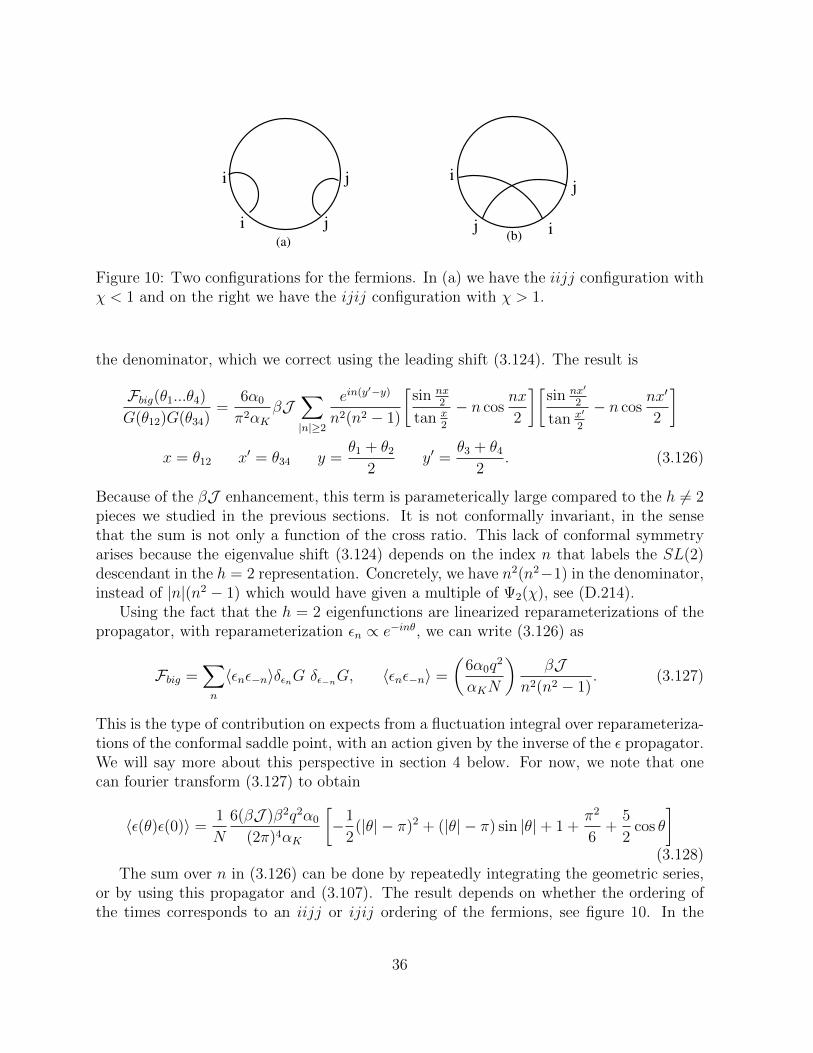
(a) (b)

j ii

i j j i

j

Figure 10: Two configurations for the fermions. In (a) we have the iijj configuration withχ < 1 and on the right we have the ijij configuration with χ > 1.

the denominator, which we correct using the leading shift (3.124). The result is

Fbig(θ1...θ4)

G(θ12)G(θ34)=

6α0

π2αKβJ

∑|n|≥2

ein(y′−y)

n2(n2 − 1)

[sin nx

2

tan x2

− n cosnx

2

][sin nx′

2

tan x′

2

− n cosnx′

2

]x = θ12 x′ = θ34 y =

θ1 + θ2

2y′ =

θ3 + θ4

2. (3.126)

Because of the βJ enhancement, this term is parameterically large compared to the h 6= 2pieces we studied in the previous sections. It is not conformally invariant, in the sensethat the sum is not only a function of the cross ratio. This lack of conformal symmetryarises because the eigenvalue shift (3.124) depends on the index n that labels the SL(2)descendant in the h = 2 representation. Concretely, we have n2(n2−1) in the denominator,instead of |n|(n2 − 1) which would have given a multiple of Ψ2(χ), see (D.214).

Using the fact that the h = 2 eigenfunctions are linearized reparameterizations of thepropagator, with reparameterization εn ∝ e−inθ, we can write (3.126) as

Fbig =∑n

〈εnε−n〉δεnG δε−nG, 〈εnε−n〉 =

(6α0q

2

αKN

)βJ

n2(n2 − 1). (3.127)

This is the type of contribution on expects from a fluctuation integral over reparameteriza-tions of the conformal saddle point, with an action given by the inverse of the ε propagator.We will say more about this perspective in section 4 below. For now, we note that onecan fourier transform (3.127) to obtain

〈ε(θ)ε(0)〉 =1

N

6(βJ )β2q2α0

(2π)4αK

[−1

2(|θ| − π)2 + (|θ| − π) sin |θ|+ 1 +

π2

6+

5

2cos θ

](3.128)

The sum over n in (3.126) can be done by repeatedly integrating the geometric series,or by using this propagator and (3.107). The result depends on whether the ordering ofthe times corresponds to an iijj or ijij ordering of the fermions, see figure 10. In the

36

non-alternating configuration iijj, we have the very simple expression

iijj order :Fbig(θ1, θ2, θ3, θ4)

G(θ12)G(π)=

6α0

π2αKβJ

(θ12

2 tan θ12

2

− 1

)(θ34

2 tan θ34

2

− 1

)(3.129)

This correlator is produced by fluctuations in the total energy in the thermal ensemble. Letus be a bit more explicit. We can compute the contribution of the energy fluctuations bystarting with the variation in the correlator produced by a small change in the temperature:

G(τ, β + δβ)

G(τ, β)= 1− 2∆

β

(1− πτ

β tan πτβ

)δβ (3.130)

Now we use the saddle point relation E = c/(2β2) to get δβ = −β3δE/c, see (2.35). Fromthe fluctuations in E we therefore expect a connected piece in the four point function thatis

1

N

Fbig(τ1, τ2, τ3τ4)

G(τ12)G(τ34)=

4

q2

(1− πτ12

β tan πτ12

β

)(1− πτ34

β tan πτ34

β

)β4

c2〈(δE)2〉. (3.131)

The energy two point function can be computed from

〈(δE)2〉 = ∂2β logZ =

c

β3. (3.132)

Inserting this, writing things in terms of θ = 2πτ/β, and converting c to αK using (5.181),we find exact agreement with (3.129).

For small θ12, (3.129) goes as θ212, suggesting the presence of a dimension two operator,

or an operator product expansion of the form ψ(θ1)ψ(θ2) ∝ (θ12)−2∆+2T (θ2). If we tookalso the θ34 → 0 limit, then we would expect to have a result proportional to 〈T (θ2)T (θ4)〉.If this was in a conformal field theory, we would have expected this to go like (sin θ24/2)−4.Instead we find that it is a constant. The the reason is that T is essentially the Hamiltonianof the theory. As such it is conserved and its two point function in the thermal ensemblesimply measures the energy fluctuations. We can write an explicit expression for T interms of ε of the form

T =NαSJ

(ε′′′ +

(2π)2

β2ε′)

+ · · · (3.133)

with αS as in (4.173). The dots indicate possible higher order terms in ε. We can thencheck using (3.128) that 〈TT 〉 is indeed constant, and is given by (3.132)

〈T (τ1)T (τ2)〉 =c

β3∝ N

β2(βJ ). (3.134)

Because of the factor of (βJ ), this becomes small in the conformal limit, seemingly inkeeping with the idea that the stress tensor should vanish in a one dimensional conformal

37

field theory. However, the contribution to the four point function also involves the threepoint couplings 〈Tψψ〉, which are the other factors in (3.131). These give two factors of(βJ ) in the numerator, which more than compensate for the suppression of 〈TT 〉.

We now turn our attention to a configuration in the alternating configuration ijij. Theresult is a bit more complicated but it simplifies nicely in the case that we take one ofthe pairs of fermions to be diametrically opposed on the circle. For example, we can takeθ3 = 0, and θ4 = π:

ijij order :Fbig(θ1, θ2, 0, π)

G(θ12)G(π)= − 6α0

π2αKβJ

(θ12

2 tan θ12

2

− 1− πsin θ1

2sin θ2

2

| sin θ12

2|

). (3.135)

This is the configuration that is appropriate for continuing to the chaos limit. To get thefunction defined in (3.95), we continue to θ2 = π

2− 2πi

βt and θ1 = θ2 − π, finding

Fbig(t)G(π)G(π)

=6α0

π2αKβJ

(1− π

2cosh

2πt

β

). (3.136)

This saturates the chaos bound.

3.3.4 Other terms from the h = 2 subspace

Because the factor k(2,n)1−k(2,n)

in (3.104) is large, of order βJ , corrections of order (βJ )−1 from

the rest of the formula (3.104) will combine to give finite contributions in the conformallimit. There are several sources of these terms. First, the δG correction to the propagatorson the LHS of (3.104) give a correction

F(θ1...θ4)

G(θ12)G(θ34)⊃ −q

2

[δG(θ12)

Gc(θ12)+δG(θ34)

Gc(θ34)

]Fbig(θ1...θ4)

Gc(θ12)Gc(θ34)(3.137)

=3α0

π2|k′c(2)|[f0(θ12) + f0(θ34)

] ∑|n|≥2

ein(y′−y)fn(x)fn(x′)

n2(n2 − 1). (3.138)

Notice that this depends on q only through the factor α0/k′c(2), which is a simple explicit

function of q. Next, we have a contribution from the first-order change in the h = 2eigenvectors, δΨ2,n. In appendix F we show that δΨ2,n is independent of q except for acoefficient of qαG. It is easy to check that this also leads to a term in F that depends onq only through the prefactor α0/k

′c(2).

Third, we have contributions from the order (βJ )0 term in k(2,n)1−k(2,n)

. This requiresknowledge of the second-order change in the eigenvalue, which we have not computed.However, we have noticed that we get a very simple final answer if we assume

k(2, n) = 1 + k′c(2)qαG|n|βJ

+k′′c (2)

2

(qαG|n|βJ

)2

+ · · · . (3.139)

38

The first term is just a restating of (3.124). One can use (3.120) to check that the secondterm is correct in the q = ∞ model. By diagonalizing the kernel constructed from thenumerical G(τ) (see appendix G), we have checked that the coefficient of the second termin (3.139) is correct to within roughly percent-level multiplicative precision, for several lowvalues of q, n. We will assume that it is actually true.

The simplification that results from (3.139) is the following. One can use (D.214) to

show that the contribution to F from the order one term in k(2,n)1−k(2,n)

combines with the

terms from the double pole at h = 2 in (3.88) and (3.90) to give, again, an expressionthat depends on q only through the prefactor α0/k

′c(2). So we conclude that up to order

(βJ )0, the four point function will be given by the Fbig contribution, plus the residues ofthe simple poles h1, h2, ... in (3.88) or (3.90), plus terms that are universal in q up to anoverall coefficient. We will compute these last terms by studying the q = ∞ four pointfunction in more detail.

3.4 More detail on the q =∞ four point function

In the q =∞ model, we can compute the four point function in way that simultaneouslytreats all of the contributions we have been discussing so far. This is based on the fact thatF is a Green’s function for a simple differential operator. Because the side-rail propagatorsin the large q kernel are proportional to sgn(θ), see (3.112), we have that

− 2

v2P 2∂θ1∂θ2K(θ1...θ4) = δ(θ13)δ(θ24), P ≡ 1

sin x2

, x = vx+ (1− v)π. (3.140)

In other words, the differential operator on the left hand side is the inverse of K. Roughly,the four point function is given by F = (K−1−1)−1. Multiplying both sides by (K−1−1),we get a differential equation for F with a delta function source.

To write the precise equation we get, it is convenient to use the coordinates x = θ12, y =θ1+θ2

2. These overcount physical configurations of points. We can reduce this overcounting

by restricting to x ≥ 0, x′ ≥ 0 and y ≥ y′. Then the correct equation is[−∂2y

4+ v2∂2

x −v2P 2

2

]F(x, y, x′, y′) = δ(y−y′)δ(x−x′)+δ(y−y′−π)δ(2π−x−x′). (3.141)

The second term on the RHS can be understood as the image of the first term under thesymmetry (x, y)→ (2π − x, y − π), see the discussion above (3.117).

We can solve this equation by separation of variables. We expand in a complete setof eigenfunctions of the operator −∂2

x + P 2/2, with boundary conditions of zero at x = 0.These eigenfunctions are just (3.117) and (3.118) with h = 2. The boundary conditionimplies that n should be an integer n ≥ 2 plus a correction of order (1− v)3 that we willneglect. Then (3.117) and (3.118) simplify to the functions fn defined in (3.109), witheigenvalues n2/4. These functions satisfy a completeness relation∑

n>2

fn(x)fn(x′)

π(n2 − 1)= δ(x− x′),

∑n>2

(−1)nfn(x)fn(x′)

π(n2 − 1)= δ(2π − x− x′). (3.142)

39

So we can write

F(x, y, x′, y′) =∑n>2

Hn(y − y′)fn(x)fn(x′)

π(n2 − 1)(3.143)[

−1

4∂2y −

v2n2

4

]Hn(y) = v [δ(y) + (−1)nδ(y − π)] . (3.144)

The factor of v on the right side came from δ(x − x′) = vδ(x − x′) and δ(2π − x − x′) =vδ(2π − x − x′). The solution for Hn(y) should be continuous and 2π-periodic. Thesources in (3.143) imply that we have a discontinuous derivative at y = 0 and y = π. Thediscontinuity at zero is equivalent to a discontinuity between the derivative at 0+ and at2π−. Solving these constraints, we find that the solution for 0 < y < 2π is

Hn(y) = − 2

n sin(nπv)

(cos [nv(y − π)] + (−1)n cos [nv(|y − π| − π)]

)(3.145)

=4 cos(ny)

πn2(1− v)+

4(y − π2) sin(ny)

πn+O(1− v) (3.146)

=

[βJ2

+ 1− (y−π2

)∂y

]4 cos(ny)

πn2+O(

1

βJ). (3.147)

In the second line we expanded in 1 − v assuming 0 < y < π. (For π < y < 2π, we needto replace the π/2 in the second term by 3π/2.) In the third line we used 1

1−v ≈βJ2

+ 1.Substituting (3.147) into (3.143) and also using fn(x) = fn(x) + (1− v)(π − x)f ′n(x) + ...,we get the full q =∞ four point function up to order (βJ )0:

F(x, y, x′, 0) =βJ − 2

[−1 + (y−π

2)∂y + (x−π)∂x + (x′−π)∂x′

] ∑|n|≥2

e−inyfn(x)fn(x′)

π2n2(n2 − 1).

(3.148)One can check that the term of order (βJ ) reproduces Fbig from (3.126) for the caseq =∞ (α0 = 2, αK = 3, G = 1

2). Although we have not displayed it here, the next term,

at order (βJ )−1 can also be computed from (3.145). Beyond that order, one has to usethe hypergeometric functions (3.117) and (3.118) that generalize fn for non-integer n.

An interesting feature of the function Fbig was that it was independent of y in thenon-alternating configuration, which corresponds to y > |x+ x′|/2. This persists at orderone, since the new y dependence of (3.148) is proportional to a y derivative of Fbig. Thisis consistent with the idea that in the q =∞ model the Hamiltonian is the only operatorthat appears in the OPE. Notice that this is rather nontrivial from the way we set upthe calculation in the previous sections: in the OPE region, the y-dependent double polecontribution in Fh6=2 must be completely cancelled by some of the terms discussed in thelast section 3.3.4.

40

3.5 Summary of the four point function

In the previous section, we argued that the order-one terms in F coming from the doublepole and the various corrections to the h = 2 contributions add up to a function thatdepends on q only through the prefactor α0/k

′c(2). We can then use the q = ∞ result

(3.148) to write the general four point function up to order one. When χ < 1, we have

F(x, y, x′, 0)

G(x)G(x′)=

= α0

6βJαK− 6

|k′c(2)|

[−1 + (y−π

2)∂y + (x−π)∂x + (x′−π)∂x′

] ∑|n|≥2

e−inyfn(x)fn(x′)

π2n2(n2 − 1)

− α0

∞∑m=1

Res

[(h− 1/2)

π tan(πh/2)

kc(h)

1− kc(h)

Γ(h)2

Γ(2h)χh2F1(h, h, 2h, χ)

]h=hm

(3.149)

For χ > 1 we have the same formula except that we need to replace Γ(h)2

Γ(2h)F (h, h, 2h, χ)→

Ψh(χ) on the second line, as in (3.88). We defined α0 in (3.50), kc in (3.73), x, x′, y in(3.126), and fn in (3.109). αK is plotted in figure 9.

In the region χ < 1, the first line is actually independent of y. It encodes the contribu-tion to the four point function from a conserved operator, T , essentially the Hamiltonianof the theory. This term is not conformally invariant. The second line represents a towerof other operators that do contribute in a conformally invariant way. The dimensions aredetermined by kc(hm) = 1.6

The expression (3.149) is very convenient for analyzing the OPE limit. If we areinterested in deriving the expression for the chaos limit, then we can start from the versionof (3.149) for χ > 1. We then replace the sum over residues by small circle contour integralsaround each point. Then we pull the contours out to h = 1

2+ is. In the process we pick up

residues at h = 2k, k ≥ 1. We have a double pole at h = 2 and single poles for k > 1. Inthe case of the single poles, we replace kc(h) by the retarded kernel kR(1− h), see (3.98).Again, we now express those contributions in terms of small contour integrals around thesepoints and shift the contour to h = 1

2+ is. After we do this, we pick up a residue at h = 2.

Thus, the final contribution involves the difference between the residues of the kc kerneland the retarded kernel

α0Res

[(h− 1

2)

π tan(πh/2)

(kc(h)

1− kc(h)− kR(1− h)

1− kR(1− h)

)Ψh(χ)

]h=2

(3.150)

This expression contains terms going like χ−1 logχ and χ−1. These should be added to

similar terms that arise from the terms involving derivatives in (3.149). The total te2πtβ

6We should also note that if (3.139) is not true, we will have further contributions, probably includinga “real” dimension two operator.

41

term, which contains the correction to the Lyapunov exponent, has the form (3.165) whichleads to (3.166). The logarithmic term that comes from the pole involving 1/(1−kc) cancelsthe one coming from the derivatives in (3.149).

3.6 The chaos exponent at finite coupling

3.6.1 The retarded kernel

One way to compute the correlator in the chaos limit is to take the exact Euclidean answerand continue it. This is the approach we took so far in the paper. If we are only interestedin getting the asympotic rate of growth, we can take a simpler approach, used by Kitaevin [8]. We will consider an out-of-time-order correlation function in real time, where thefermions are separated by a quarter of the thermal circle:

F (t1, t2) = Tr[y ψi(t1)y ψj(0)y ψi(t2)y ψj(0)

], y ≡ ρ(β)1/4. (3.151)

The 1/N piece of F is determined by a set of ladder diagrams on a time contour thatincludes the thermal circle and also a pair of real-time folds for the operators ψ(t1) andψ(t2). As t1, t2 become large, these folds grow. The asymptotic growth rate of the 1/Npiece of F is determined only by the properties of the ladder diagrams on real-time partof the contour. To analyze these ladders, we define a retarded kernel

KR(t1...t4) = J2(q − 1)GR(t13)GR(t24)Glr(t34)q−2. (3.152)

Here, GR are the retarded propagators, which include the sum over insertions on the twosides of the fold. The function Glr is a Wightman correlator with points separated by halfof the thermal circle in addition to the real time separation. In the conformal limit

GR(t) = 2b cos(π∆)θ(t)

[π

β sinh πtβ

]2∆

, Glr(t) = b

[π

β cosh πtβ

]2∆

. (3.153)

The growth rate of F is determined by the condition that adding one rung to the ladder willnot change the sum. This means that F must be an eigenfunction of KR with eigenvalueone:

F (t1, t2) =

∫dt3dt4KR(t1...t4)F (t3, t4). (3.154)

To solve this, we make a growth ansatz

F (t1, t2) = eλL(t1+t2)/2f(t12) (3.155)

and then determine the values of λL such that we can find an f that gives an eigenfunctionof KR with eigenvalue one, solving (3.154). In the conformal limit, one can show by directintegration that we have eigenfunctions and eigenvalues

e−hπβ

(t1+t2)[cosh π

βt12

]2∆−h , kR(h) =Γ(3− 2

q)Γ(2

q− h)

Γ(1 + 2q)Γ(2− 2

q− h)

. (3.156)

42

This agrees with the definition of kR(h), given previously in (3.98). As we noted there,the only solution to kR(h) = 1 is h = −1, which gives λL = 2π

β. One might have expected

to also find subleading growth rates in the conformal limit, corresponding to differentfamilies of eigenfunctions. Such eigenfunctions exist, but one can check that the nextlargest allowed value of λL is zero. This explains why every growing term in the chaoslimit was growing at this rate, including various terms that were subleading to the enhancedcontribution Fbig.

3.6.2 Large q

In the large q model we can use this retarded kernel to find the growth exponent λL at allvalues of the coupling. From (2.14) and the definition of GR in (2.13), together with theanalytic continuation to real times τ → β/2 + it of (2.18), we find that

GR(t) = θ(t), qJ2Glr(t)q−2 =

2π2v2

β2 cosh2(πvβt). (3.157)

where v was defined in (2.19). v goes from zero at weak coupling to one at strong coupling.Substituting (3.157) into the formula for the retarded kernel, and then taking derivatives∂t1∂t2 of equation (3.154) with the ansatz (3.155), we get[

λ2L

4− ∂2

x

]f(x) =

2π2v2

β2 cosh2(πvβx)f(x). (3.158)

After rescaling the x variable, the equation becomes

−(λLβ

2πv

)2

f(x) =

[−∂2

x −2

cosh2 x

]f(x), x =

πv

βx, f(x) = f(x). (3.159)

This is a Schrodinger problem for a particle in the −2/ cosh2 x potential. There is a singlebound state f ∝ 1/ cosh x. The energy of this state is minus one, which gives the exactgrowth exponent

λL =2π

βv. (3.160)

At weak coupling we have λL ≈ 2J , and at strong coupling we have λL ≈ 2πβ

[1− 2/(βJ )].We give a plot of λL in figure 11.

3.6.3 General q

For general q, we do not have an exact expression for λL at finite coupling. However,we can relate the first (βJ)−1 correction to the parameter αG, and we can compute thefunction at small and moderate βJ numerically. First we discuss the (βJ)−1 correction.One way to compute this is to do first order perturbation theory in the retarded kernel. Theleading non-conformal correction to KR comes from plugging (3.122) into the definitions

43

10 -1 10 0 10 1 10 2

β J

0

0.2

0.4

0.6

0.8

1q = 4

10 -1 10 0 10 1 10 2

β J

0

0.2

0.4

0.6

0.8

1λ

*β/2π

large q

Figure 11: Left: the exact λL in the large q model. Right: λL for q = 4. The redcurve shows the formula (3.166) in a region of reasonable validity. The circles are exactvalues, obtained by numerically solving real-time Schwinger-Dyson equations and thendiagonalizing the retarded kernel. Note that the x axis is βJ , not βJ .

GR(t) = [G(it+ε)−G(it−ε)]θ(t) and Glr(t) = G(it+β/2) to get the corrected propagators

δGR

GR

= − αGβJ

(2−

π tan πq

+ 2πtβ

tanh πtβ

),

δGlr

Glr

= − αGβJ

(2− 2πt

βtanh

πt

β

). (3.161)

Rather than taking this direct approach, we will use the results derived earlier in thissection to get the answer by a different method. From (3.136), the leading term in thechaos limit behaves like

F(t)

G(π)G(π)≈ −3α0βJ

2παKe

2πβt. (3.162)

If we correct the growth exponent to λL = 2πβ

+ δλL, and expand to linear order in δλL,we expect a term linear in t times the growing exponential:

Fexpect(t)G(π)G(π)

= − (tδλL) · 3α0βJ2παK

e2πβt. (3.163)

We expect δλL to be of order (βJ )−1, so this term is of order one at large coupling. Wefound a term exactly of this type when we analyzed the double pole in the chaos limit ofthe Fh6=2 function. The contribution that contains the log is

Fhave(t)G(π)G(π)

= − 3α0

k′R(−1)π2∂hΨh(χ)|h=2 (3.164)

≈ 3α0

2πk′R(−1)

2π

βte

2πβt (3.165)

44

where we took the large t limit in the second line, using (3.96) and (3.100). Comparingwith (3.163), and rewriting αK in terms of αG using (3.125), we find

λL =2π

β

(1− −k

′(2)

k′R(−1)

qαGβJ

+ ...

). (3.166)

We have checked that this agrees with the direct method described above.The correction is always negative. It is consistent with the large q exact result. Evalu-

ating the derivatives and plugging in the numerical value for αG, we have that when q = 4

−k′(2)

k′R(−1)

qαGβJ≈ 4.28

βJ≈ 6.05

βJ, (q = 4). (3.167)

When q approaches two, the correction diverges, like

−k′(2)

k′R(−1)

qαGβJ

=6π

(π2 − 6)(q − 2)

1

βJ, (q → 2). (3.168)

This divergence seems to be consistent with the fact that the q = 2 the model is free, sothe chaos exponent must vanish for any value of βJ .

Another approach to computing λL is to numerically solve the real-time Schwinger-Dyson equations to find GR and Glr, and then use binary search to find the largest valueof λL such that there exists an eigenfunction f(t12) that satisfies (3.154). This works wellfor small and moderate βJ . In figure 11 we plot some data points for q = 4 computedthis way. They appear to match smoothly to the large (βJ ) result (3.166). We will givea few more details about this approach in appendix G.

4 The effective theory of reparameterizations

In this section we will discuss the effective action of the model. This gives a secondperspective on the computation of the four point function that makes some features clearer,such as the physical interpretation of the enhanced h = 2 contribution. It also allows usto connect the specific heat term in the free energy to the ladder kernel.

The effective action of the model is derived by starting with the original fermion pathintegral and doing the Gaussian integral over the disorder. This gives a bilocal action forthe fermions. One can integrate out the fermions after introducing a field G(τ1, τ2) and a

Lagrange multiplier field Σ that sets G equal to 1N

∑j ψj(τ1)ψj(τ2). We are left with the

nonlocal action [1]

S

N= −1

2log det(∂t − Σ) +

1

2

∫dτ1dτ2

[Σ(τ1, τ2)G(τ1, τ2)− J2

qG(τ1, τ2)q

](4.169)

for G, Σ. This is an exact rewriting of the theory. Because of the Lagrange multiplierconstraint, we can compute the four point function of fermions (3.40) in the G, Σ variables

45

as1

N2

∑ij

〈ψi(τ1)ψi(τ2)ψj(τ3)ψj(τ4)〉 =

∫dΣdG e−SG(τ1, τ2)G(τ3.τ4). (4.170)

The action has a saddle point at the solutions G, Σ of the Schwinger Dyson equations(2.6). (Note that G, Σ denote the integration variables in (4.170), while G,Σ are theclassical solutions to the action (4.169)). Evaluating the integrand at this saddle pointgives the disconnected part of the four point function. We can also consider fluctuations.It is convenient to define the fluctuations g, σ so that we have G = G + |G| 2−q2 g and

Σ = Σ + |G| q−22 σ. Notice that the measure is invariant dGdΣ = dgdσ. Expanding the

action to second order in g, σ and using the saddle point equation G = (∂τ − Σ)−1 tosimplify, we find

S

N= − 1

4J2(q−1)

∫dτ1...dτ4 σ(τ1, τ2)K(τ1...τ4)σ(τ3, τ4)

+1

2

∫dτ1dτ2

[g(τ1, τ2)σ(τ1, τ2)− 1

2J2(q−1)g(τ1, τ2)2

]. (4.171)

Here, K is the symmetric ladder kernel defined in (3.47). We can integrate out σ, gettingan action just for g:

S

N=J2(q−1)

4g · (K−1 − 1)g. (4.172)

We can use this to get the 1/N term in the four point function (4.170), by replacing

both factors of G in the integrand by |G| 2−q2 g and then doing the Gaussian integral withan appropriately chosen contour. This immediately gives the expression (3.104) that wepreviously derived from the Feynman diagrams.

The expressions written so far are valid at any energy. When we go to low energies andwe use the conformal expressions, Gc,Σc in order to evaluate the kernel K, then we findthat the action is zero when evaluated on fluctuations that are reparameterizations of theconformal correlator, as in (3.107). This is because these fluctuations are eigenfunctions ofthe kernel with eigenvalue one (3.108). More conceptually, it is because the action (4.169)is reparametrization invariant (under (2.8)) if we drop the ∂t term inside the determinant.Notice that even though the action is reparametrization invariant, the solution Gc is onlyinvariant under the SL(2, R) subgroup. Thus we can view reparametrization invarianceas an emergent symmetry of the infrared theory which is spontaneously broken by theconformal solution Gc. The zero modes in the action can be viewed as Nambu-Goldstonemodes for the spontaneous breaking of the full conformal symmetry down to SL(2, R).Note that we could consider an alternative model which does not have a reparametrizationinvariance, then we do not get any enhanced contribution in the IR, see appendix (H).

We can now include the leading non-conformal to the action (4.172), which is deter-mined by the first order shift in the h = 2 eigenvalues of the kernel (3.124). This willprovide a non-zero action for these reparametrization modes. To compute this, we con-sider a small reparameterization τ → τ + ε(τ), and evaluate the action on δεGc. It is

46

2 4 6 8 10 12 14 16 18 20q

0

0.005

0.01

0.015

αS

Figure 12: The coefficient of the Schwarzian action αS is plotted. The blue curve is thevalue given by the previously computed αG. The circles are values inferred from (5.181)and the numerical evaluation of the specific heat c. The agreement is a check that theSchwarzian action is correct nonlinearly, not just for small reparameterizations.

convenient to work in frequency space for ε, and to use that reparameterizations δεGc areproportional to the h = 2 eigenfunctions of the kernel. We get an action proportional ton2(n − 1), where n labels the Matsubara frequency. This factor arises from the productof the |n| in the eigenvalue shift and the |n|(n2 − 1) in the normalization of the h = 2eigenfunctions. The result, in position space, is

S

N=αSJ

∫ β

0

dτ1

2

[(ε′′)2 −

(2π

β

)2

(ε′)2

], αS ≡

αK6q2α0

=q|k′c(2)|αG

6q2α0

. (4.173)

This action for ε is local, even though the original action is nonlocal. This is reasonablebecause the breaking of reparameterization invariance is a UV effect. In fact, the actionthat we get could have been guessed by standard effective field theory reasoning: it isthe simply the expression of lowest order in derivatives that vanishes for global SL(2)transformations. It must vanish in that case because the correlator is SL(2) invariant,δSL(2)Gc = 0 is zero. Notice that these SL(2) reparameterizations should not be thoughtof as zero modes, they simply are not part of the functional integral over G.

Therefore the emergent conformal symmetry is both spontaneously broken by the in-frared solution Gc as well as explicitly broken, which gives a small action (4.173). It issmall in the sense that it formally vanishes as J → ∞. On the other hand, notice that itis large in the sense that it is of order N . To get a reasonable theory we need to include theeffects of this breaking. This pattern of symmetry breaking is reminiscent to the pions inQCD, the chiral symmetry is both spontaneously and explicitly broken (by the quark massterms). Thus (4.173) turns the reparametrization modes into Pseudo-Nambu-Goldstonebosons.

The enhanced contribution Fbig from (3.126) can now be understood in a simple way.It is the result of the part of the functional integral (4.170) that consists of summing over

47

reparameterizations of the circle weighted by the action (4.173). This leads directly to(3.127).

We would like to generalize the action (4.173) to finite reparameterizations τ → f(τ).It is convenient to start with the zero temperature case where both f and τ are coordinateson the line. f is a coordinate on the “straight” line where the IR correlator is a pure power,and τ is a coordinate on the reparameterized line. Near any point (we take the origin),one can write

f(τ) = f(0) + f ′(0)

(τ +

1

2

f ′′(0)

f ′(0)τ 2 + ...

). (4.174)

For small τ we have a small reparameterization with ε′ = 0 and ε′′ = f ′′/f ′, followed bya scaling and translation. The scaling and translation have no effect on the correlator onthe zero temperature line, so we can generalize

1

2

∫dτ(ε′′)2 → 1

2

∫dτ

(f ′′

f ′

)2

(4.175)

which up to a total derivative implies that the action can be written as

S = −NαSJ

∫dτf, τ, f, τ ≡ f ′′′

f ′− 3

2

(f ′′

f ′

)2

. (4.176)

In the second step we introduced the Schwarzian derivative f, τ and used integration by

parts. Note that the Schwarzian derivative is invariant under SL(2) symmetry f → (af+b)(cf+d)

.This is an exact symmetry since the zero temperature Gc is exactly invariant under thistransformation.

To get the action for reparameterizations of the circle, we consider the transformation

f(τ) = tan

(πτ

β

)(4.177)

which maps the circle to the line. Already for this transformation we get an interestingresult. Inserting (4.177) into the Schwarzian action (4.176) we get a finite temperaturecorrection to the free energy

−βF ⊃ NαSJ

∫ β

0

dτtanπτ

β, τ = 2π2αS

N

βJ. (4.178)

At large q, we have αS = 14q2 (αK = 3 and α0 = 2), and this agrees with the term found

previously in (2.32). For q = 2 we get αS = 124π

( α0 = π2, αK = π), and again weagree with (2.34). In figure 12 we give a plot of αS and indicate a numerical check of thisformula. Note that while this action nicely explains the near extermal entropy, it saysnothing about the zero temperature entropy.

48

If we are interested in further reparametrizations of the circle, τ → g(τ), we can usethe composition law for the Schwarzian derivative f(g(τ)), τ = (g′)2f, g + g, τ toobtain

S

N= −αS

J

∫dτtan

πg(τ)

β, τ =

αS2J

∫dτ

[(g′′

g′

)2

−(

2π

β

)2

(g′)2

]. (4.179)

Writing g(τ) = τ + ε(τ) and expanding in ε we get both of the quadratic terms in (4.173).

5 The density of states and the free energy

The large N free energy is determined by evaluating the G, Σ action (4.169) on the saddlepoint values G,Σ. In a low temperature expansion, we have

logZ = −βE0 + S0 +c

2β+ · · · , (5.180)

where the ground state energy, entropy and specific heat are all proportional to N . Theground state energy will not be important for our discussion. The zero temperature entropyis given for general q by (2.33). The specific heat is determined by (4.178) as

c

2= 2π2αS

N

J. (5.181)

For the case q = 4 we have c ≈ 0.396N/J .All of the terms in (5.180) are proportional to N . There is an important order-one

correction to this free energy which we can compute from the determinant of the quadraticaction (4.171). The log determinant of this action gives a term7

−βF ⊃ −1

2

∑h,n

log[1− k(h, n)]. (5.182)

We get an interesting log βJ term from the h = 2 modes, which have eigenvalues close toone. Substituting in the corrected eigenvalues (3.124), we get

−βF ⊃ −∞∑n=2

logn

βJ+ const.→ #βJ − 3

2log βJ + const. (5.183)

This sum is divergent, but the divergence will presumably be cut off at n ∼ βJ , whereone expects higher order effects to make the eigenvalue k(2, n) small. This will lead to aterm proportional to βJ with an unknown coefficient; this is a correction to the ground

7This contribution to the free energy was first pointed out by J. Polchinski and A. Streicher, usingFeynman diagrams. They also noted that the sum over near-zero-modes would lead to a log term [27].

49

state energy. The special feature of the h = 2 sum is that we also get the finite log pieceindicated on the right. This can be extracted by zeta function regularization or the EulerMacLaurin formula. The logarithm means that the partition function is proportional toβ−3/2 at large β.

We can also get this factor of β−3/2 from the action (4.173) as follows. We also do thefunctional integral over ε(τ). However, we need to recall that we are not integrating overSL(2, R) transformations. Thus, we need to divide the integral by the volume of SL(2, R),since we should view SL(2, R) as a gauge symmetry. This will result in the insertion offactors of the form δ(ε(0))δ(ε′(0))δ(ε′′(0)) in the functional integral. When we rescale ε toget rid of the coefficient of the quadratic action in (4.173), we will find a factor of (βJ )−3/2

from the three delta functions.The integral over all the non-zero modes with h 6= 2 will produce a βJ divergence that

corrects the ground state energy, plus a β-independent factor which can be absorbed as a1/N correction to S0 in (5.180).

With this information, we can now compute the density of states by doing an inverseLaplace transform to the partition function. It is convenient to subtract the ground stateenergy, so that from now on E indicates the energy above the ground state. The integralis

ρ(E) =1

2πi

∫γ+iR

dβZ(β)eβE ∝ eS0

∫dβ

(βJ)32

eβE+c/2β ≈√

2π

cJ3eS0+

√2cE . (5.184)

In the final step we approximated the integral by saddle point, valid for cE 1. It isinteresting that the determinant from the saddle point integral cancels the factor β−

32 from

the one-loop free energy, so ρ(E) approaches a constant at low energy, in this approxima-tion. We can also compute the integral for small cE, where it becomes ≈ 4

√πE/J3eS0 .

The√E vanishing is interesting, because it agrees with the behavior that one gets for the

spectrum of a random Hamiltonian. However, we cannot trust the computation for suchsmall values of E; at the crossover point cE ∼ 1, the saddle point in the β integral is atβ ∼ c ∼ N/J . At such low temperatures, the Schwarzian action discussed in the previoussection stops being semiclassical, and our analysis would need to be improved8.

A somewhat complementary approach to the spectrum is to exactly diagonalize theHamiltonian (2.2) for small values of N . The Majorana fermion operators ψi are justmatrices that satisfy ψi, ψj = δij. In other words, they are Dirac gamma matrices. Torepresent the model with N fermions, we need a Hilbert space of dimension 2N/2. We wereable to study up to N = 32 without any special techniques. We give a plot of the binnedspectrum for N = 32 in figure 13.

8As a side remark, note that, as we discuss in[26], the effective action (4.173) also appears for nearextremal black holes. Thereore in such cases the computation of (5.184) will be valid. In that case, thefact that the density is constant at low energies is consistent with the fact that BPS black holes can havea large degeneracy at exactly zero energy. For non-BPS black holes we could have further corrections thatmight remove the large degeneracy at exactly zero energy.

50

-2 -1 0 1 2

Energy, in units of J

0

50

100

150

200

250

300

350

400

Nu

mb

er

of e

ige

nva

lue

s

Eigenvalues for N=32, plotted with 300 bins

Figure 13: The spectrum for a single realization of the q = 4 model with N = 32 fermions.

One obvious feature of the plot is that there is no scale-invariant divergence ρ(E) ∝ 1/Eor δ(E) at low energy. Instead, the density goes smoothly to zero. A naive reading of theplot suggests that the spectrum vanishes as Ep with p near one. The zero temperatureentropy does not reflect any actual degeneracy, only a large density of states near theground state. From this perspective, a completely random Hamiltonian on a system ofN qubits also has a zero temperature entropy, S0 = N log 2, from the density ρ(E) ∝√E(E − 2)2N . This gives a low temperature free energy logZ = N log 2− (3/2) log β.In fact, from the plot (13), the density of states in SYK does not look too different

from the random matrix semicircle. It is important to note, though, that if we increaseN the density in the central region will be growing much faster than near the edges.Near the center, we expect the density characteristic of the infinite temperature entropy,ρ ∼ 2N/2 ≈ e0.35N , while near the edges we expect eS0N ≈ e0.23N . By diagonalizing theHamiltonian for different values of N between 24 and 32, and counting the number of levelswithin bands of width 0.3J , we found the best fit e0.33N near the center and e0.24N nearthe edge, in reasonable agreement with large N expectations. Note that the Hamiltonian,while containing of order N4 random elements is not as random as a general random matrixin Hilbert space, which would contain 2N random elements.

6 Towards a bulk interpretation

A natural starting point for a bulk interpretation is the action (4.169). Due to the large

factor of N , this looks like a classical system for the fields Σ and G. One of them can beeasily eliminated, so we really have one field which is a function of two variables. Thuswe seem to have a field theory defined on a two dimensional space. It is natural to thinkof the average of the two times as a time and the difference as a new dimension. The

51

solution to the Schwinger Dyson equations gives us a classical background for this system,and then we have fluctuations governed by a quadratic action of the form (4.172). Thecomputation of the four point function of the fermions can be viewed as the computationof the propagator for this bilocal field and it involved inverting the operator (1/K − 1)(4.172).

In the large βJ limit, we have seen that there is a dominant mode associated to theemergence of a conformal symmetry which is both spontaneously and explicitly broken. Aconformal symmetry is easily obtained if we consider AdS2 gravity. When we regularizethe space and we introduce some boundary conditions we get a boundary mode that isthe same as the one parametrized by the function f(τ) discussed above. The AdS2 metricpreserves explicitly an SL(2, R) group. This metric is spontaneously breaking the rest ofthe reparametrizations. The boundary mode is the corresponding Goldstone boson andit implies that pure AdS2 gravity is not well defined, if we want to have any non-trivialexcitation [34, 35, 7]. However, when AdS2 arises from a higher dimensional theory, thereis always a coupling to a dilaton which is not constant on AdS2. This explicitly breaks theconformal symmetry and it gives rise to an action for the modes parametrized by f(τ).The details of this will be discussed in a separate publication [26] and the discussion isvery closely related to the analysis in [7]. In summary, both the mode parametrized byf(τ) and its action are reproduced by any near AdS2 (or NAdS2) geometry. This featureis insensitive to the precise details about the type of matter we can have in AdS2. It resultspurely from the emergence of the conformal symmetry and its slight breaking.

In order to elucidate the kind of matter we have in the dual of SYK we need to look atthe other propagating modes contained in the field G(τ1, τ2). Fortunately, for all the othermodes we can use the SL(2, R) symmetry to describe them. The propagating modes canbe read off from the OPE expansion of the fermion four point function. Their conformaldimensions are the solutions to kc(hm) = 1 and were discussed in section 3.2.6. We get aninfinite tower of dimensions which asymptotes to (3.93) (3.94) at large values of m. Thisasymptotic form of the dimensions has a structure that looks like a two particle state inAdS2. However, it is important to note that the shift in dimensions is of order one, andnot order 1/N . Therefore, we cannot view these states as a two particle state of fermionsin the bulk with weak, gravitational strength, interactions. This tower of particles isreminiscent of a string theory with a string scale of order the AdS radius. In fact, it alsolooks similar to what we would get in an O(N) model, where we get a state for each spinand the number of single string states does not exhibit an exponential growth with energy(Hagedorn behavior). Here all members of the tower are getting an order one shift in theirdimensions9. In two dimensions we do not have a clear notion of spin, but if we definespin by the contribution to the correlator in the chaos region, then they have spins S > 2(S = 2 is for the h = 2 states related to the reparametrizations).

9In the free O(N) models we get such a tower with dimensions given exactly by the sum of dimensionsof the two elementary free field components ψ∂2n+1ψ. In the case of the Gross Neveu model in 2 + 1dimensions, interactions give the lowest member gets an anomalous dimension. Namely ψ2 has a shiftfrom ∆free = 2 → ∆ = 1.

52

6.1 Comments on kinematic space.

In this subsection we expand a bit on the comment on the relation between the two timesof G and the two variables of a bulk field. Recently, this was further explored in [18].

In general we can define

t =τ1 + τ2

2, σ =

τ1 − τ2

2(6.185)

At this point this is just a simple relabeling of the times. Written in this way, we see thatsome of the terms in the action (4.169) become local in the t, σ space. But the Pfaffianterm is still non-local.

Furthermore, in the IR region, the Casimir operator acting on the two times τ1, τ2 hasthe form

C12Φ = −(τ1 − τ2)2∂τ1∂τ2Φ = σ2(−∂2t + ∂2

σ)Φ = ∇2Φ (6.186)

where Φ(t1, t2) = δGGc

where δG is a small fluctuation around the classical solution of theaction (4.169), which in the IR is given by the conformal answer Gc (2.9). We see thatthis looks like the laplacian in AdS2, in coordinates ds2 = −dt2+dσ2

σ2 , and in units wherethe AdS radius is set to one. This space was defined in a purely kinematic way by usinggeneral properties of the conformal group. It was called kinematic space in [29, 30]. Notethat even the quadratic action (4.172) for Φ is highly non-local. It involves 1/kc(h) − 1which is a complicated function of the casimir, C = h(h− 1) = ∇2, see (3.73). We shouldthink of this Φ as describing many degrees of freedom since there are many solutions of1/kc(h)− 1 = 0, describing the tower of states in section (3.2.6).

It is amusing to note that the expression for the energy given in (2.27) looks like anADM like expression for the energy in terms of a property of the solution at the boundaryof the geometry, namely τ1 = τ2 or σ = 0.

In the Euclidean theory we expect the bulk to be H2. However, the kinematic spacedefined as above, through the Casimir operator, continues to be a Lorentzian signaturespace. This is a general feature of the Casimir operator acting on bilocal fields as hasbeen used recently in [30]. We can view the space as dS2, or AdS2 with time periodicallyidentified, depending on the overall sign we choose for this metric. More explicitly, inthe Euclidean finite temperature theory, we have the times τ1 and τ2 which are periodicvariables. When we define the sum and the difference we get (for β = 2π)

τ =τ1 + τ2

2, σ =

τ1 − τ2

2, C = sin2 σ(−∂2

τ + ∂2σ) (6.187)

which looks like the wave equation on global dS2, or AdS2 with time periodically identified.In fact, the funny set of eigenfunctions that we needed to sum over in e.g. (3.83) has asimple interpretation in AdS2 or dS2. They are the set of normalizable solutions of thiswave equation. We had a further anti-symmetry restriction on the wavefunctions, whichamounts to antisymmetry under an anti-podal transformation in this dS2 or AdS2 space.It would be interesting to see if some variation of this model has a de-Sitter interpretation.

53

Finally, this relation to kinematic space suggests that the usual bulk of AdS/CFT requiresa further inverse X-ray or Radon transform. We make a few more comments on this inappendix I.

6.2 The fermions

So far, we have avoided the “elephant in the room”, which are the N boundary fermions.One can question whether these should correspond to N bulk fermions or not. Beforetrying to answer this question, let us recall the special case of q = 2. In that case the Nboundary fermions give rise to just one “bulk” fermion as follows. After we diagonalizethe random mass matrix by an orthogonal transformation we find that φi =

∑m rimψm,

where ψm is a fermion with a definite mass (or frequency)10. In the large N limit, thedistribution of masses is nearly continuous and we can view it as an extra dimension. So,in this case we see that the different boundary fermions ψi give rise to different parts of thebulk fermion field ψ. This should be the case, since a bulk fermion has many independentcreation and annihilation operators.

Before we continue, let us also make another general comment. One can imagine gettingrid of the fundamental fermions by viewing the couplings jijkl as dynamical with very slowdynamics so that they are effectively constant [19]. At the order we are working, this givesthe same equations 11. Once we make the couplings jijkl dynamical, we can gauge theO(N) symmetry. Naively this seems to remove the fermions from the spectrum so that wedo not need to discuss them further. However, we continue to have a related operator ofthe form

O(τ, τ ′) = ψi(τ)[Pei

∫ ττ ′ A] j

iψj(τ

′) (6.188)

The one point functions of this operator 〈O(τ, τ ′)〉 ∼ NG(τ, τ ′) continue to display anSL(2, R) invariant form with dimensions ∆.

We can now wonder what the interpretation of such an operator in the bulk is. Thisquestion was studied in detail for the related case of a matrix model in the non-singletsector in [37]. In that case, the corresponding state was a folded closed string coming fromthe boundary into the bulk. In our case we can imagine a similar explanation in terms ofan open string that comes in from the boundary.

Then we can view the propagating states as strings oscillating in AdS2, see figure 14.This is just a picture, since we are not displaying the precise string theory background.

We can now go back to the ungauged model. At the level that we treated it so far, ithas a global O(N) symmetry. And it is tempting to think that whether or not we gauge thesymmetry is some operation purely at the boundary. Therefore even for the O(N) model

10For positive m we have a complex creation operator and for negative m the corresponding annihilationoperator.

11Except that there is an additional contribution to the free energy from the j fields, of the form Nq log βfrom the j fields. We thank S.H. Shenker for this comment. This model is structurally reminiscent of the2+1 dimensional O(N) theories with fundamental bosons and fermions studied in [36].

54

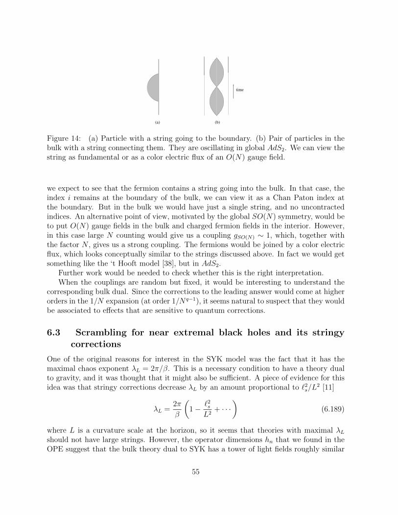
time

(a) (b)

Figure 14: (a) Particle with a string going to the boundary. (b) Pair of particles in thebulk with a string connecting them. They are oscillating in global AdS2. We can view thestring as fundamental or as a color electric flux of an O(N) gauge field.

we expect to see that the fermion contains a string going into the bulk. In that case, theindex i remains at the boundary of the bulk, we can view it as a Chan Paton index atthe boundary. But in the bulk we would have just a single string, and no uncontractedindices. An alternative point of view, motivated by the global SO(N) symmetry, would beto put O(N) gauge fields in the bulk and charged fermion fields in the interior. However,in this case large N counting would give us a coupling gSO(N) ∼ 1, which, together withthe factor N , gives us a strong coupling. The fermions would be joined by a color electricflux, which looks conceptually similar to the strings discussed above. In fact we would getsomething like the ‘t Hooft model [38], but in AdS2.

Further work would be needed to check whether this is the right interpretation.When the couplings are random but fixed, it would be interesting to understand the

corresponding bulk dual. Since the corrections to the leading answer would come at higherorders in the 1/N expansion (at order 1/N q−1), it seems natural to suspect that they wouldbe associated to effects that are sensitive to quantum corrections.

6.3 Scrambling for near extremal black holes and its stringycorrections

One of the original reasons for interest in the SYK model was the fact that it has themaximal chaos exponent λL = 2π/β. This is a necessary condition to have a theory dualto gravity, and it was thought that it might also be sufficient. A piece of evidence for thisidea was that stringy corrections decrease λL by an amount proportional to `2

s/L2 [11]

λL =2π

β

(1− `2

s

L2+ · · ·

)(6.189)

where L is a curvature scale at the horizon, so it seems that theories with maximal λLshould not have large strings. However, the operator dimensions hn that we found in theOPE suggest that the bulk theory dual to SYK has a tower of light fields roughly similar

55

to a string spectrum with `s ∼ RAdS. This seems to be a counterexample to the idea thatmaximal chaos implies a gravity dual. This motivates us to examine in more detail theform of the scale L that was appearing in (6.189).

Let us briefly review the shock wave calculation that gives the chaos limit of the fourpoint function. We have an out of time ordered four point function with two pairs ofoperators. One pair is at time zero, and the other is at time t. The growing part of thecorrelator is given by the phase shift of the bulk field associated to the t = 0 pair as itcrosses a shock sourced by the other pair. The general form of the shock wave plus staticblack hole metric is

ds2 = −a(uv)dudv + b(uv)dxidxi + h(x)δ(u)du2 (6.190)

where we have added D − 2 extra flat dimensions. Einstein’s equations give

12

[−∂2

i

b−(∂u∂vbab

)(D − 2)

]h(x)δ(u) = 8πGNTuu (6.191)

12

[−∇2 + φ′′(0)

φ(0)

]h(x)δ(u) = 8πGNTuu (6.192)

where φ ∝ bD−2

2 is the “dilaton”, or the coefficient of the two dimensional curvature inthe action

∫φR(2) after dimensional reduction on the extra flat coordinates. And φ′′ is

the second derivative with respect to proper distance from the horizon, evaluated at thehorizon. Now we integrate this over the transverse space and also over u in a neighborhoodof the horizon. We get

1

2

φ′′

φAh = 8πGNPu. (6.193)

where A is the area of the horizon, and h is the zero mode of the shock wave profile. Puis the momentum of the quantum associated to the pair of operators at time t, which is

Pu ∼ (∆/RAdS)e2πβt. Dividing both sides by 2GN gives

φ′′

φSh = 4πPu (6.194)

where S is the entropy of the black hole. The phase shift for the other field crossing thisshock is

δ ∼ ∆

RAdS

h ∼[

∆2

R2AdS

φ

φ′′

]1

Se

2πβt. (6.195)

We should regard the quantity in brackets as being the βJ enhancement. In fact, fornear extremal black holes, we have that the profile of the dilaton at the horizon has theform φ = φ0 + γ cosh ρ

RAdS2, where φ0 gives the extremal entropy and γ the near extremal

entropy, with γ φ0. So we can write

R2AdS

φ′′

φ=S − S0

S0

−→ ∝ 1

q2βJ(6.196)

56

where on the left side we have a gravity expression and on the right hand side we write thequotient of entropies that we have in the SYK model. Here we have simply reproduced theleading part of the answer from a gravity computation. We will connect it more clearly tothe reparametrizations in [26]. The prefactor enhancement of the butterfly effect for nearextremal black holes was noticed previously in [39, 40].

Now we consider stringy corrections to the chaos exponent, following [11]. We readthese off from (6.192). We reintroduce the extra dimensions, substitute

k2 → k2 +φ′′

φ(6.197)

in the Regge behavior of the flat space string amplitude s2−`2sk2/2, and then take k to zero.This gives an effective spin which is

j = 2− `2s

2

φ′′

φ= 2− `2

s

2R2AdS

(S − S0)

S. (6.198)

So even if the string length is large, there is another parameter suppressing the correctionto

λL =2π

β(j − 1) =

2π

β

(1− `2

s

2R2AdS

S − S0

S+ · · ·

). (6.199)

Note that using the expression for the ratios of entropies in (6.196) we get an estimate forthe SYK model of a correction of order 1

q2βJ (provided `s ∼ RAdS). This is indeed what

we found in (3.166) up to q dependent factors.It is a little surprising that the change in the Regge spin can be small, despite the

presence of light strings. The right interpretation seems to be that the gravity contributiongets a βJ (or near-extremal) enhancement, but the higher stringy exchanges do not. Sogravity dominates and we have a spin near two.

7 Brief Conclusions

The SYK model is an interesting quantum mechanical model displaying a spontaneouslyand explicitly broken reparametrization symmetry. These features dominate the low energyproperties of the model and are expected to be universal for any large N system withemergent reparametrization symmetry. One motivation to study this model is that nearextremal black holes also display this pattern of symmetry breaking [26]. We also expectthat this will be relevant to other condensed matter physics models. This symmetrybreaking pattern gives rise to several features of the low energy dynamics. First, it givesrise to a specific heat that is linear in the temperature. It also gives rise to a largecontribution to the four point function, which saturates the chaos bound in the out oftime ordered configuration. All these features are expected to be universal features ofsystems with emergent reparametrization symmetry or NCFT1s.

57

We also studied several features that are special to this particular model, such asthe spectrum of dimensions of fermion bilinear operators. These suggest that the dualdescription should contain a single Regge trajectory with low tension strings in nearlyAdS2 space. We also gave a detailed description of the non-enhanced parts of the fourpoint function. Several questions remain about the proper holographic interpretation ofthis particular model.

Acknowledgements

We thank D. Anninos, A. Kitaev, J. Polchinski, S. Shenker and Z. Yang for discussions.J.M. is supported in part by U.S. Department of Energy grant de-sc0009988. D.S. issupported by the Simons Foundation grant 385600.

A The Schwinger-Dyson equations and the kernel

We consider the Schwinger Dyson equations (2.6). We treat the iω term as a pertubation.In fact for an arbitrary perturbation we can write the equations as

G ∗ Σ +G ∗ s = −1 = −δ(t− t′′) , Σ = J2Gq−1 (A.200)

where the ∗ stands for G ∗ Σ =∫dt′G(t, t′)Σ(t′, t′′) and G is the full solution with the

source. The source induced by the −iω term in (2.6) is s = −δ′(τ − τ ′) We can now writeG = Gc + δG, where δG is the perturbation to the conformal solution induced by thepresence of the source.

Expanding the equations to first order, using the second equation to express δΣ interms of δG, and convolving with G on the right, we obtain

δG− (q − 1)J2Gc ∗Gq−2c δG ∗Gc = Gc ∗ s ∗Gc (A.201)

(1−Kc)δG = −∫dτ ′∂τGc(τ − τ ′)Gc(τ

′ − τ ′′) (A.202)

where we have used the homogeneous equation Gc ∗ Σc = −δ(τ − τ ′′).The right hand side has the form sgn(τ−τ ′′)

|τ−τ ′′|4∆ . This has the form of a function like (3.69)with t0 →∞ and h→ −2∆. Therefore seems that all we need would be to invert 1−Kc.However, kc(−2∆) = ∞ (see (3.73)). This would lead to δG = 0. However, we couldhave terms that obey (1 − Kc)δG = 0. A formal solution would be an h = −1 modewhich gives the correction δG ∝ Gc

1|τ−τ ′| (see again (3.69) with τ0 →∞). This is formally

annihilated by 1−Kc, but it is not actually annihilated because of UV divergences. TheseUV divergences arise from the region where the two times in the integral are very close toeach other. This region would be regulated in the full theory and has the form of the righthand side of (A.202). Furthermore, it has the right J dependence to match the right handside. This also shows that in order to compute the full coefficient, we need to know the

58

whole flow, in order to know how the coincident point divergence of the conformal case isregulated.

Another point of this appendix is to show that the same kernel that appears in thefour point function also appears when we want to compute the corrections around the IRsolution.

B The kernel as a function of cross ratios

The kernel gives the (n+1)-ladder diagram in terms of the n-ladder diagram as

sgn(τ12)sgn(τ34)

|τ12|2∆|τ34|2∆Fn+1 (χ) = − 1

α0

∫dτadτb

sgn(τ1a)sgn(τ2b)

|τ2b|2∆|τ1a|2∆|τab|2−4∆· sgn(τab)sgn(τ34)

|τab|2∆|τ34|2∆Fn (χ)

χ =τ12τ34

τ13τ24

χ =τabτ34

τa3τb4. (B.203)

We would like to use conformal symmetry to turn this into a one-dimensional integralequation. We can take τ1 = 0, τ3 = 1, τ4 = ∞, so that χ = τab

τa−1and χ = τ2, and then

replace the τb integration variable by χ. The measure is dτadτb = dτadχ(1− τa). One finds

Fn+1(χ) =1

α0

∫ ∞−∞

dχ

|χ|2

(|χ||χ||χ− χ|

)2∆

sgn(χχ)m(χ, χ)Fn(χ) (B.204)

m(χ, χ) = sgn(χ− χ)

∫ ∞−∞

dτsgn(τ)sgn(1− τ)sgn(1− 1−χ

χ−χτ)

|τ |2∆|1− τ |1−2∆|1− 1−χχ−χτ |2∆

. (B.205)

The integral over τ can be done by dividing up the region of integration and using∫ 1

0

dτ

(1− xτ)aτ b(1− τ)c=

Γ(1− b)Γ(1− c)Γ(2− b− c) 2F1(a, 1− b, 2− b− c, x). (B.206)

The answer is

m(χ, χ) ≡

2π

sin 2π∆F (1− 2∆, 2∆, 1, z)−B2∆

(1

1−z

)−B1−2∆

(1

1−z

)z ≤ 0

− 2πz2∆ sin 2π∆

F (2∆, 2∆, 1, z−1z

) + 2πsin 2π∆

F (2∆, 1− 2∆, 1, z) 0 ≤ z ≤ 1

− 2πsin 2π∆

F (2∆, 1− 2∆, 1, 1− z) +B2∆(z−1) +B1−2∆(z−1) 1 ≤ z.

z ≡ 1−min(χ, χ)

|χ− χ|, Bh(x) =

Γ(h)2

Γ(2h)xh2F1(h, h, 2h, x). (B.207)

We are interested in applying this integral kernel to functions F(χ) with the symmetryof the four point function. This means that we should have F(χ) = F(χ/(χ − 1)). Thistransformation maps the interval between zero and two into the complement on the realline, so we can restrict our attention to f(χ) with 0 ≤ χ ≤ 2. Using the invariance andchanging integration variables in (B.204), we get a closed equation in this interval:

Fn+1(χ) =1

α0

∫ 2

0

dχ

χ2Fn(χ)

[χ2∆χ2∆

|χ− χ|2∆m(χ, χ) + sgn(χ− 1)

χ2∆χ2∆

|χ+ χ− χχ|2∆m(χ,

χ

χ− 1)

].

(B.208)

59

The expression in brackets times 1/α0 is the kernel Kc(χ, χ) described in (3.59).

C Representing F0 in terms of Ψh

Using contour manipulations very similar to the one we used to derive (3.88) and (3.90),it is possible to write a formula for F0 as a sum over residues. There are two differences:first, we do not have a divergent term at h = 2, so we do not need to subtract it. Second,since we have kc(h) in the integrand instead of kc(h)/[1− kc(h)], we are interested in thepoles of kc(h), which occur at values h = 2

q+ 1 + 2n. We get the following formulas for

F0. When χ > 1,

F0(χ) = −α0

∞∑n=0

Res

[(h− 1/2)

π tan(πh/2)kc(h)Ψh(χ)

]h= 2

q+1+2n

χ > 1. (C.209)

and when χ < 1 we have

F0(χ) = −α0

∞∑n=0

Res

[(h− 1/2)

π tan(πh/2)kc(h)

Γ(h)2

Γ(2h)χh2F1(h, h, 2h, χ)

]h= 2

q+1+2n

χ < 1.

(C.210)These expressions (C.209) and (C.210) can be checked by numerically evaluating theresidue sums and comparing to (3.80).

D Writing Ψh(χ) in terms of Ψh,n(θ1, θ2)

By solving the casimir differential equation, one finds that the antisymmetric eigenfunc-tions of C1+2 with weight ∆ = 1/2 and symmetry under (x, y) → (2π − x, y + π) are

Ψh,n(θ1, θ2) = γh,ne−iny

2 sin x2

ψh,n(|x|), x = θ12, y =θ1 + θ2

2. (D.211)

where the functions ψh,n are the ones appearing in (3.117) and (3.118), but with v = 1 sothat n = n. The norms of the continuum eigenfunctions h = 1/2 + is can be determinedby assuming that 〈Ψh,n,Ψh′,n〉 = 2πδ(s−s′), where the inner product is defined in (3.102),and analyzing the integral near x = 0 and x = 2π, as in (3.78). One finds an expressioninvolving a product of gamma functions. With these normalizations, we have that

2h− 1

π tan(πh)

Ψh(χ)

(2 sin θ12

2)(2 sin θ34

2)

= 2∑n

Ψ∗h,n(θ1, θ2)Ψh,n(θ3, θ4), χ =sin θ12

2sin θ34

2

sin θ13

2sin θ24

2

.

(D.212)which shows that the continuum part of the formulas (3.83) and (3.104) agree. Whenwe go to the discrete case where h is an even integer, the continuum normalization γ2

h,n

60

diverges for |n| ≥ h, and the factor of 1/ tan(πh) in (D.212) also diverges. The coefficientof this divergence gives the relation

2h− 1

π2

Ψh(χ)

(2 sin θ12

2)(2 sin θ34

2)

= 2∑|n|≥h

Ψ∗h,n(θ1, θ2)Ψh,n(θ3, θ4) (D.213)

where the Ψh,n are now defined with discrete norms so that 〈Ψh,n,Ψh′,n′〉 = δhh′δnn′ . Thisestablishes the equivalence of the discrete parts of (3.83) and (3.104). A special case thatwe use in the main text of the paper is

Ψ2(χ) = 2∑|n|≥2

ein(y−y′)fn(x)fn(x′)

|n|(n2 − 1). (D.214)

where x = θ12, y = θ1+θ22

, x′ = θ34, y′ = θ3+θ42

and χ is defined as in (D.212). The functionsfn were defined in (3.109).

E Direct approach to the shift in eigenvalue

In this appendix we sketch a second derivation of (3.125), which consists of substitutingG+δG in for the propagators in the kernel, with δG given in (3.122), and then analyzing the

integrals to compute 〈Ψ2,n, δK ·Ψ2,n〉. When we correct the propagator, we get corrections

to K of two types. One type is a correction to the rung propagators, see figure 4. In thatcase, we can use the fact that Ψ2,n is an eigenfunction of the unperturbed kernel to dotwo of the integrals. This gives an expression that is independent of q, up to an overallmultiple (q − 2)αG. Comparing to the q =∞ case, one finds that in general

δrungk(2, n) = −(q − 2)αGβJ

3|n|2. (E.215)

The corrections to the rail propagators are not as simple. The change in the kernel is

δrailK = −J2(q − 1)|G(θ12)|q−2

2 δG(θ13)G(θ24)|G(θ34)|q−2

2 + (13↔ 24). (E.216)

Our first goal is to show that 〈Ψ2,n, δrailK · Ψ2,n〉 is proportional to |n|. We can do thisusing conformal symmetry. It will be useful to represent the function f0 appearing in(3.122) as an integral

f0 =

∫ π

−πdθ0

| sin θ10

2sin θ20

2|

| sin θ12

2|

. (E.217)

This implies that δG has the form of an integrated conformal three point function of twofermions with an operator of dimension minus one. Another useful identity is based on

1

8

sin2 θ12

2

sin2 θ10

2sin2 θ20

2

=∞∑n=2

einθ0e−inyfn(x), for |eiθ0| < 1, (E.218)

61

which implies that Ψ2,n is proportional to an integrated conformal three point function oftwo fermions with a dimension two operator:

Ψ2,n(θ1, θ2) =γn4π

∫ 2π

0

dθ0 e−inθ0 2 sin θ12

2

(2 sin θ10

2)2(2 sin θ20

2)2, γ2

n =3

π2|n|(n2 − 1). (E.219)

Here the integral is defined by giving θ0 a small imaginary part iε sgn(n).

The shift 〈Ψ2,n, δrailK · Ψ2,n〉 is an integral over four times θ1, ..., θ4 of a product ofpropagators and eigenfunctions. The idea is to represent the eigenfunctions Ψ2,n and thechange in the propagator δG using the integral formulas (E.219) and (E.217). This addsthree new integration variables, θa, θb, θc. The complete expression is proportional to theintegral over all seven θ variables of

γ2nein(θa−θb)

∣∣∣∣∣sin θ12

2sin θ34

2

sin θ13

2sin θ24

2

∣∣∣∣∣2∆

sgn(θ12θ34θ13θ24)

sin2 θ1a2

sin2 θ2a2

sin2 θ3b2

sin2 θ4b2

∣∣∣∣∣sin θ1c2

sin θ3c2

sin θ13

2

∣∣∣∣∣ (E.220)

plus a similar term with (13 ↔ 24). First we consider holding θa, θb, θc fixed and doingthe integral over θ1, ...θ4. The θa and θb variables are the integration parameters in therepresentation (E.219) of Ψ2,n. They should be understood as having small imaginaryparts of opposite sign. With this prescription, the integral over θ1...θ4 is convergent, andhas analytic dependence on θa and θb. (The naive divergence of the integral θ13 = 0 is notpresent becuase of the sgn(θ13) factor.) Now, the important point is that the integral isSL(2) covariant, with external weights h = 2 for the θa, θb variables and weight h = −1for the θc variable. So the answer must be proportional to

γ2nein(θa−θb) sin θac

2sin θbc

2

sin5 θab2

. (E.221)

We cannot have absolute value signs or sgn functions in this expression, because it musthave analytic dependence on θa, θb. Finally, we integrate over the last three variables. Theintegral over θc turns the numerator into cos θab/2. In the integral over θa, the opposite iεprescriptions for θa, θb imply that we pick up the residue of the fifth order pole at θa = θb.This is proportional to n2(n2 − 1). Combining with the factor γ2

n defined in (3.109) we

conclude that 〈Ψ2,n, δrailK ·Ψ2,n〉 is indeed proportional to |n|.To determine the coefficient of proportionality, one can compute the ratio of the rung

and rail corrections by analyzing the integrals at large n. More precisely, we take n largeand β large, with Ω = 2πn/β held fixed. In this limit it is better to use a proper timecoordinate on the circle, τ , rather than the angle θ = 2πτ/β. The h = 2 eigenfunctions(3.109) are proportional to

Ψ(τ1, τ2) ∝ eiΩ(τ1+τ2)/2

τ12

f(Ωτ12/2), f(ρ) = cos ρ− sin ρ

ρ. (E.222)

62

For large n, all integrals will be dominated by the UV, where the propagator and correctionare

Gc = bsgnτ

|τ |2∆,

δG

Gc

∝ 1

|τ |. (E.223)

The frequency Ω scales out, so we can choose the value Ω = 2. Then the rung and railcontributions to the eigenvalue are proportional to the integrals

Irail =

∫dτ2dτ3dτ4e

iτ2−iτ3−iτ4f(τ2)sgn(τ2)

|τ2|2−2∆

sgn(τ34)

|τ34|2−2∆

sgn(τ3)

|τ3|1+2∆

sgn(τ24)

|τ24|2∆f(τ34) (E.224)

Irung =q − 2

2

∫dτ2dτ3dτ4e

iτ2−iτ3−iτ4f(τ2)sgn(τ2)

|τ2|3−2∆

sgn(τ34)

|τ34|2−2∆

sgn(τ3)

|τ3|2∆

sgn(τ24)

|τ24|2∆f(τ34)

(E.225)

where the proportionality constant is the same in both cases. Since we know the normalizedrung contribution, we can get the full answer by computing the ratio of the above integralsand using (E.215):

δk(2, n) =

(1 +

IrailIrung

)δrungk(2, n), (E.226)

The rung integral is easy to evaluate using the fact that we started with eigenvectors ofthe original kernel. The rail integral takes more work (it is convenient to represent someof the factors in the integrand as fourier transforms) but the integrals can be done, andone eventually finds agreement with (3.125).

F The first order change in h = 2 eigenvectors

In this appendix we show that the the first order shift in the h = 2 eigenvectors Ψexact2,n =

Ψ2,n + δΨ2,n + ... is independent of q up to an overall multiple:

δΨ2,n =qαG

2δΨq=∞

2,n . (F.227)

Morally, the reason is the following. The h = 2 eigenvectors are given by reparameteriza-tions of Gc, and the first order corrections are related to reparameterizations of δG, whichitself is univesal in q up to a coefficient. However, we will not need this interpretation. Togive the actual argument, we start by considering the reparameterization δεI, where

I(τ1, τ2) =

∫dτadτbG(τ1, τa)Σ(τa, τb)G(τ2, τb). (F.228)

Here, reparameterizations are defined to act as in (3.107), and we consider the functionI to have weight ∆ = 1/q. With this definition, I is reparameterization covariant, inthe sense that the reparameterization of the answer for the integral is the same as the

63

reparameterization of the various parts that go inside the integral. Writing this statementout for linearized reparameterizations and using the exact Schwinger-Dyson equations∫

dtaG(t1, ta)Σ(ta, t2) = −δ(t12) + ∂t2G(t1, t2), (F.229)

we find

(1−K) · δεG =1

qHε, Hε(τ1, τ2) ≡

∫dτ ε′(τ)G(τ1, τ)∂τG(τ2, τ)− (1↔ 2). (F.230)

This is true for any value of the coupling, provided that K and G are the exact kerneland propagator. Using K = |G| q−2

2 K|G|− q−22 , and taking a matrix element with one of the

conformal eigenvectors Ψh,n, we get (the inner product is as in (3.102))

〈Ψh,n, (1− K) · |G|q−2

2 δεG〉 =1

q〈Ψh,n, |G|

q−22 Hε〉. (F.231)

Naively, the leading piece of the LHS of (F.231) is at order (βJ)−1, where we use the

conformal answers for everything. However, this gives zero because |Gc|q−2

2 δεGc is an

eigenvector of Kc with eigenvalue one. In fact, the leading IR terms are at order (βJ)−2.We get these by substituting in either δG or δK into the left side. The RHS has no termsat this order, so these contributions must cancel:

〈Ψh,n, (1− Kc) · δε(|Gc|q−2

2 δG)〉 − 〈Ψh,n, δK · |Gc|q−2

2 δεGc〉 = 0. (F.232)

The integral defining the LHS of (F.232) has a UV divergence; we define the integral bytaking only the cutoff-independent (βJ)−2 piece and discarding the power divergence. Inthe exact theory, UV divergences in this expression and on both sides of (F.231) will beregulated to terms at order (βJ)−h and (βJ)−h−1. Depending on h these might dominateover the IR term we are interested in, but as long as h 6= 2 they can be separated.

Let us examine (F.232) in more detail. We can act with the kernel to the left, giving

(1−kc(h). Now, |Gc|q−2

2 δεGc is proportional to (1/q) times an h = 2 conformal eigenvector,and the quantity being reparameterized in the LHS is independent of q, up to a multipleαG. So we conclude that

1

qαG

〈Ψh,n, δK ·Ψ2,n〉1− kc(h)

(F.233)

is independent of q. Apart from the prefactor, this expression is the first order perturbationtheory formula for the matrix element of 〈Ψh,n, δΨ2,n〉, so we conclude (F.227). Althoughwe did not need explicit formulas for the corrected eigenvectors in this paper, one can getthem by expanding and normalizing (3.117) and (3.118).

64

1 2 3 4 5 6θ

0

0.1

0.2

0.3

0.4

0.5

0.6

G

β J = 10

1 2 3 4 5 6θ

0

0.1

0.2

0.3

0.4

0.5

0.6

G

β J = 50

Figure 15: The exact G(θ) in the q = 4 model is shown in solid lines, for βJ = 10 (left)and βJ = 50 (right). We also plot the conformal answer Gc in dash-dotted lines, and theconformal answer plus the first correction Gcf0 in dashed lines.

G Numerical solution of the SD equations

In this appendix, we discuss the numerical solution of the Schwinger-Dyson equations atfinite βJ . The euclidean solutions give us the coefficient αG (and thus also αK , αS). Onecan also use these solutions to directly compute the large N free energy. The real-timesolutions were used to compute the blue circles in (11).

We will begin by discussing the euclidean equations, at finite temperature:

G(ωn)−1 = −iωn − Σ(ωn), Σ(τ) = J2G(τ)q−1. (G.234)

Here ωn = 2π(n+ 1/2)/β is a Matsubara frequency. One can solve these equations just byiterating them, starting with the free correlator and using a numerical fourier transform toswitch betwen frequency ωn and time θ = 2πτ/β. In order to get the iteration to converge,one should take a weighted update12

Gj(ωn) = (1− x)Gj−1(ωn) + x1

−iωn − Σj−1(ωn). (G.235)

where the weighting x is a parameter. One can set it by beginning with x = 0.5 andthen monitoring the difference

∫|Gj − Gj−1|2 between successive steps. If this begins to

increase, one divides x by a half and continues the iteration. Some exact solutions areshown for different values of βJ in figure 15.

For large values of βJ , the difference between the exact and conformal correlators isfit very well by

G ≈ Gc −αGβJ

Gcf0 (G.236)

12We are grateful to A. Kitaev for suggesting this.

65

where f0 was defined in Eq. (3.121) and αG is a fitting parameter. More precisely, thisholds as long as τJ is large. We determine αG from the numerical solutions by fittingfor the coefficient in the region π/2 ≤ θ ≤ π. In the numerics we have a finite frequencycutoff and finite J , but we take both large and look for convergence. For small q < 3 toget accurate results we have to extrapolate in both variables, first in the cutoff and thenin J .

The function αG(q) was plotted in figure 9. Some explicit values are αG(2) = 0, αG(4) ≈0.1872, αG(6) ≈ 0.1737, αG(8) ≈ 0.1522, and αG(10) ≈ 0.1336. A Pade approximant thatstays within approximately one percent of the numerical answer is

αG(q) ≈ 2(q − 2)

16/π + 6.18(q − 2) + (q − 2)2. (G.237)

With the solution to the Schwinger-Dyson equations, we can also compute the free en-ergy using (2.26). In terms of the correlators and the self energy at Matsubara frequencies,we have

logZ

N=

1

2log 2 +

1

2

∞∑n=−∞

log

[1 +

Σ(ωn)

iωn

]− β

2

∫ β

0

[Σ(τ)G(τ)− J2

qG(τ)q

]. (G.238)

To get this expression from (2.26), we have used the free answer logZ = N2

log 2 in thecase J = 0 to set the constant. The effect was to replace∑

n

log(−iωn)→ log 2. (G.239)

The answer we expect for the free energy is an expansion in powers of 1/(βJ):

logZ

N= a1βJ + a2 +

a3

βJ+ ... (G.240)

where −a1J is the ground state energy density, a2 is the zero temperature entropy density,and 2a3 is the specific heat density. We can remove the ground state energy by considering

logZ − J∂J logZ

N= a2 + 2

a3

βJ+ ... (G.241)

The derivative term can be evaluated using (2.27). Evaluating the sum of these terms onthe numerical solution to the Schwinger Dyson equations for moderately large βJ , we findvery good agreement with the S0(q) given in (2.33). The agreement is good enough thatwe can subtract S0 and study the remainder for different values of βJ in order to computea3. This was used to compute the circles in figure 12.

We can also continue the equations (G.234) to get the retarded and Wightman correla-tors in real time, following [13]. For this it is important to use the spectral function ρ(ω).Here, ω with no subscript is a real-time frequency, which takes continuous values. We are

66

using conventions where the spectral function can be defined as the real part of the fouriertransform of the retarded propagator:

ρ(ω) ≡ 2ReGR(ω) = G>(ω)(1 + e−βω), G>(t) ≡ 〈ψ(t)ψ(0)〉 = G(it+ ε). (G.242)

The Matsubara propagator G(ωn) can be written in terms of ρ as

G(ωn) =

∫dω′

2π

ρ(ω′)

−iωn + ω′. (G.243)

In this form, one can easily continue to complex frequency. The continuation to real-timefrequency is essentially the retarded propagator: GR(ω) = −iG(−iω + ε). To get thereal-time Schwinger-Dyson equation we also have to understand how to continue Σ(ωn).Writing the second equation (G.234) in frequency space and using (G.242) we have

Σ(ωn) = J2

∫ β

0

eiωnτG(τ)q−1, G(τ) =

∫dω

2πe−ωτ

ρ(ω)

1 + e−βω. (G.244)

After doing the τ integral we get an equation that can be continued to complex frequency,

Σ(ωn) = J2

∫ [q−1∏j=1

dωj2π

ρ(ωj)

1 + e−βωj

]1 + e−β

∑j ωj

−iωn +∑

j ωj. (G.245)

Now we have a closed set of equations for ρ that can be iterated. First, we compute theretarded propagator from the continuation of the first equation in (G.234):

GR(ω)−1 = [−iG(−iω + ε)]−1 = −iω + ε− iΣ(−iω + ε) (G.246)

Next, we compute the spectral function by taking twice the real part. Finally, we substituteρ into (G.245) to get the new self energy. An appropriately weighted iteration of thisprocedure converges. In implementing these equations numerically, we have to put bothan IR cutoff and a UV cutoff on the frequencies. This makes the problem more challengingthan the Euclidean problem, but we still get good agreement with the conformal answerand the leading correction. See figure 16 for a plot.

The only place we used these real-time solutions in the main text was to compute thecircles in figure 11. To evaluate these we solve the above equations to get GR and Glr,which can also be written in terms of ρ. We then assume an ansatz (3.155). This turns(3.154) into a one-dimensional integral equation for f(t12). This can be discretized andrepresented as a matrix equation. λL is determined by the condition that this matrixshould have an eigenvalue equal to one. We find this by doing binary search.

H A model without the reparametrization symmetry

It is natural to ask whether there is a model where instead of 1/(1−K) in the expressionfor the four point function (3.45) we get 1/(1 − gK), with a g < 1. This would move

67

0 2 4 6 8 10 122π t/ β

0

0.05

0.1

0.15

0.2

0.25

0.3

Glr

2 4 6 8 102π t/ β

0

0.2

0.4

0.6

0.8

1

GR

Figure 16: The retarded propagator GR (left) and the half-circle Wightman correlator Glr

(right) are plotted in the q = 4 model with βJ = 10. The solid curve is the numericalanswer, the dash-dotted curve is the conformal answer, and the dashed curve is the con-formal answer plus the leading correction (3.161). The behavior of the numerical GR neart = 0 is somewhat contaminated by finite-cutoff wiggles.

the pole away from h = 2 and would lead to finite expression in the conformal limit. Itis clear from our discussion in section 4 that this can only be true in a model withoutreparametrization symmetry.

A simple model with these properties arises if we assume that the couplings ji1···iq aretime dependent fields with a two point function

〈ji1···in(t)ji1···in(0)〉 =J2(q − 1)!

N q−1× 1

|t|2α(H.247)

The new factor is the last one. In the limit α→ 0 we recover the original model (to leadingorders in the 1/N expansion).

With this modification we can still write the Schwinger Dyson equations as

1

G(ω)= −iω − Σ(ω) , Σ(τ) = J2[G(τ)]q−1 1

|τ |2α(H.248)

In the low energy limit, we can now make a scale invariant ansatz as before

Gc =b sgn(τ)

|τ |2∆(H.249)

With this ansatz we can solve the low energy limit of (H.248) (dropping the iω term) andwe find that

∆Σ = ∆(q − 1) + α = 1− ∆ , ∆ =1− αq

(H.250)

where we have denoted the dimension of Gc by ∆, since it is not equal to 1/q. The overallcoefficient has exactly the same expression as before (2.10) in terms of ∆

J2bqπ = (1

2− ∆) tanπ∆ (H.251)

68

We can now consider the kernel that appears in the four point function computation.It has an expresssion similar to the one before (3.44),

Kc(τ1, τ2; τ3, τ4) = −(q − 1)Gc(τ13)Gc(τ24)Σc(τ34)

Gc(τ34)

= −(q − 1)bqJ2 sgn(τ13)

|τ13|2∆

sgn(τ24)

|τ24|2∆

1

|τ34|2−4∆

= − (q − 1)

( 1

∆− 1)

Kc,∆ (H.252)

where Kc,∆ is the usual kernel but with ∆ → ∆. Namely, in (3.49) (3.50) we replace

∆→ ∆ and q → 1/∆.The eigenvalues of the new kernel are then equal to

kc(h) = gkc,∆(h) , g ≡ (q − 1)

( 1

∆− 1)

(H.253)

where k∆(h) is the usual expression in terms of ∆ (i.e. we replace 1/q → ∆ everywhere in

(3.73).) Now if 0 < α < 1, then we see that ∆ < 1/q which means that that g < 1. Thisimplies that now the sum that appears in the computation of the four point function isregular and of the form

1

1− K=

1

1− gK∆

(H.254)

Therefore now we do not have to worry about the h = 2 contribution. For h = 2we find that K = g < 1 and the sum is finite. In this case, the expression analogous to(3.83) is finite. Since k′c(h = 2) < 0, the first pole is at a value hp < 2. Something similar

happens with the retarded kernel, KR where the pole moves to a value −1 < hchaos < 0.More explicitly, using the formula (3.98) we find

kR(1− h) =cos π(∆− h

2)

cos π(∆ + h2)kc,∆(h) (H.255)

We can easily check from here that kR(h = 0) = q − 1 > 1 and that kR(h = −1) = g < 1.Therefore there is always a solution for kR(hchaos) = 1 for −1 < hchaos < 0, leading to the at

behavior e(−hchaos) 2πβt. This means that we have a growing contribution but growing more

slowly than the bound. Here we are assuming that when we go to the finite temperaturetheory we also change the two point function (H.247) to its finite temperature version.

As α → 0, it seems clear that we will get a divergence that will go like 1/α. Thecoefficient of this divergence would be a function of cross ratios. This is different than thefunction that multiplies 1

βJ that we discussed in section (3.3.3).As we take the α → 0 the sum over the normalizable h = 2 modes, in Fourier space,

involves a factor of the form 1/(1− K) ∝ 1/(α + n(βJ)

), where we also included the terms

69

that would break the conformal symmetry when α = 0. Then depending on whether α or1/(βJ) is larger, we go from one regime to the other.

We can then derive an effective action for reparametrizations which would reproducethe above kernel. We find that it should have the schematic form∑

n

[1

Jβn2(n2 − 1) + α(n2 − 1)|n|

]|εn|2 (H.256)

the last term in the action is non-local. It should come from the variation of the modifiedterm in the effective action ∫

dθ1dθ2J2

|2 sin θ12

2|2αGc(θ12)q (H.257)

when we make a reparameterization of Gc and then expand to quadratic order in ε. Whenα is zero, the term is reparameterization invariant, but one can check that if we expandto linear order in α it does give the second term in (H.256).

We could view the two point function of the j’s as arising from a higher dimensionalconformal field theory. If that field theory has a holographic dual, then we would bedescribing something that lives on an AdS2 subspace of a higher dimensional bulk. Sucha theory would not have a purely dynamical two dimensional gravity. This setup arisesnaturally in the Kondo model and its holographic duals. See [41] for a Kondo modelexample that inspired the SYK model studied in this paper, and [42] and references thereinfor holographic examples.

I Further coments on Kinematic space

In this appendix we expand a bit more on the comments in section 6.1, where we exploredproperties of the two dimensional space characterized by two times t1, t2 of a bilocal field.

We can consider the finite temperature Lorentzian theory. After defining the followingcoordinates the Casimir becomes (setting β = 2π)

t =t1 + t2

2, σ → t1 − t2

2, → C → sinh2 σ(−∂2

t + ∂2σ) (I.258)

where we now have the wave equation on the outside of the Lorentzian black hole. We seethat the two point function Gc is determining the metric of the space we should consider.

We can easily get to the interior by taking t1 → t1 + iβ/4, t2 → t2 − iβ/4 so that nowwe get

C ∼ cosh2 σ(∂2t − ∂2

σ) (I.259)

which is the wave operator in the interior region. The fact that we have a complex shiftin the two times by t1− t2 → t1− t2 + iβ/2 is related to the fact that we can easily createparticles in the interior if we have access to both sides of the thermofield double, or if weperform small perturbations of the thermofield double state [43].

70

Finally, there is an elegant relation between bulk and boundary using embedding co-ordinates. Points on the boundary can be written in terms of projective coordinatesXM = (X−1, X0, X1), with (X.X) ≡ −X2

−1−X20 +X2

1 = 0 and X ∼ λX. If we have a pairof such points on the boundary, Xa

M and XbM , then we can define

Y L =εMNLXa

MXbN

(Xa.Xb)(I.260)

where (Xa.Xb) is simply the inner product using the SL(2) metric. This obeys (Y.Y ) = −1.Of course, conceptually, this is the same as what we have discussed above, except thatnow we see that the formulas are SL(2) covariant.

I.0.1 The kinematic space in the full model at q =∞

As a final comment, we will consider the case of of q →∞. This case looks simpler becausethe only state in the singlet spectrum is the h = 2 state. As we approach the q → ∞limit the other states are decoupling, but their enegies are not becoming large. In thissense it is different than the very large ‘t Hooft coupling limit of a gauge theory, wherethe decoupling of the string states happens because they become heavy. An observation isthat in this case we get an interesting picture in terms of the “bulk” coordinates definedin (6.185). In this limit the kernel is given by

K(t1, t2; t3, t4) = sgn(t13)sgn(t24)1

(|t34|+ ε)2− (3↔ 4) , ε =

1

J(I.261)

We then find that it obeys the equation

− (|t12|+ ε)2∂t1∂t2K(t1, t2; t3, t4) = [δ(t1 − t3)δ(t2 − t4)− (3↔ 4)]= (σ + ε)2(−∂2

t + ∂2z )K(t, z; t′, z′) (I.262)

where we defined t, σ as in (6.185). After defining z = σ + ε we find that we get thewave operator in AdS2 (parametrized by t, z) with a cutoff at z = ε. In particular, herez ≥ ε always and, for the spectral problem we are putting boundary conditions that setthe normalizable functions to be zero at z = ε. So in this case the kernel is really K = 2

∇ε ,see also (3.76), where ∇ε is the laplacian in AdS2 with dirichlet boundary conditions atz = ε. Now the quadratic term in (4.172) becomes 1

K−1 = 1

2∇2ε −1 and has a simple local

form. This is interesting because popular way to regularize AdS computations consistsin setting a cutoff a z = ε. However, it was unclear which kind of regularization of theboundary theory would give such a cutoff. Here we see an example, where we get thesame kind of regularized AdS2 problem. In this theory we flow rather quickly from thetopological theory in the UV to the IR AdS2-like theory. This needs to be taken with agrain of salt given that we do not know whether there is a way to think about the modelas a local theory in AdS. Also the above construction seems more related to regulatingthe kinematic space than the actual bulk.

In the finite temperature case we also get a dS2, or AdS2 with periodic time. In thiscase we also need to rescale the size of the circles relative to their naive values, see (3.114).

71

References

[1] A. Kitaev, “A simple model of quantum holography.”http://online.kitp.ucsb.edu/online/entangled15/kitaev/,http://online.kitp.ucsb.edu/online/entangled15/kitaev2/. Talks at KITP, April7, 2015 and May 27, 2015.

[2] J. L. Karczmarek, J. M. Maldacena, and A. Strominger, “Black hole non-formationin the matrix model,” JHEP 01 (2006) 039, arXiv:hep-th/0411174 [hep-th].

[3] I. R. Klebanov, “String theory in two-dimensions,” in Spring School on StringTheory and Quantum Gravity (to be followed by Workshop) Trieste, Italy, April15-23, 1991. 1991. arXiv:hep-th/9108019 [hep-th].

[4] S. Sachdev and J.-w. Ye, “Gapless spin fluid ground state in a random, quantumHeisenberg magnet,” Phys. Rev. Lett. 70 (1993) 3339, arXiv:cond-mat/9212030[cond-mat].

[5] S. Sachdev, “Holographic metals and the fractionalized Fermi liquid,” Phys. Rev.Lett. 105 (2010) 151602, arXiv:1006.3794 [hep-th].

[6] V. de Alfaro, S. Fubini, and G. Furlan, “Conformal Invariance in QuantumMechanics,” Nuovo Cim. A34 (1976) 569.

[7] A. Almheiri and J. Polchinski, “Models of AdS2 backreaction and holography,”JHEP 11 (2015) 014, arXiv:1402.6334 [hep-th].

[8] A. Kitaev. http://online.kitp.ucsb.edu/online/joint98/kitaev/. KITPseminar, Feb. 12, 2015.

[9] S. H. Shenker and D. Stanford, “Black holes and the butterfly effect,” JHEP 03(2014) 067, arXiv:1306.0622 [hep-th].

[10] A. Kitaev. Talk given at the Fundamental Physics Prize Symposium, Nov. 10, 2014.

[11] S. H. Shenker and D. Stanford, “Stringy effects in scrambling,” JHEP 05 (2015)132, arXiv:1412.6087 [hep-th].

[12] J. Maldacena, S. H. Shenker, and D. Stanford, “A bound on chaos,”arXiv:1503.01409 [hep-th].

[13] O. Parcollet and A. Georges, “Non-fermi-liquid regime of a doped mott insulator,”Phys. Rev. B 59 (Feb, 1999) 5341–5360.http://link.aps.org/doi/10.1103/PhysRevB.59.5341.

[14] S. Sachdev, “Bekenstein-Hawking Entropy and Strange Metals,” Phys. Rev. X5no. 4, (2015) 041025, arXiv:1506.05111 [hep-th].

72

[15] P. Hosur, X.-L. Qi, D. A. Roberts, and B. Yoshida, “Chaos in quantum channels,”JHEP 02 (2016) 004, arXiv:1511.04021 [hep-th].

[16] W. Fu and S. Sachdev, “Numerical study of fermion and boson models withinfinite-range random interactions,” arXiv:1603.05246 [cond-mat.str-el].

[17] Y.-Z. You, A. W. W. Ludwig, and C. Xu, “Sachdev-Ye-Kitaev Model andThermalization on the Boundary of Many-Body Localized Fermionic SymmetryProtected Topological States,” arXiv:1602.06964 [cond-mat.str-el].

[18] A. Jevicki, K. Suzuki, and J. Yoon, “Bi-Local Holography in the SYK Model,”arXiv:1603.06246 [hep-th].

[19] J. Polchinski and V. Rosenhaus, “The Spectrum in the Sachdev-Ye-Kitaev Model,”arXiv:1601.06768 [hep-th].

[20] D. Anninos, T. Anous, and F. Denef, “Disordered Quivers and Cold Horizons,”arXiv:1603.00453 [hep-th].

[21] D. Anninos, T. Anous, P. de Lange, and G. Konstantinidis, “Conformal quivers andmelting molecules,” JHEP 03 (2015) 066, arXiv:1310.7929 [hep-th].

[22] N. Goheer, M. Kleban, and L. Susskind, “(1+1)-dimensional compactifications ofstring theory,” Phys. Rev. Lett. 92 (2004) 191601, arXiv:hep-th/0310120[hep-th].

[23] D. A. Roberts and D. Stanford, “Two-dimensional conformal field theory and thebutterfly effect,” Phys. Rev. Lett. 115 no. 13, (2015) 131603, arXiv:1412.5123[hep-th].

[24] S. Jackson, L. McGough, and H. Verlinde, “Conformal Bootstrap, Universality andGravitational Scattering,” Nucl. Phys. B901 (2015) 382–429, arXiv:1412.5205[hep-th].

[25] G. Turiaci and H. Verlinde, “On CFT and Quantum Chaos,” arXiv:1603.03020

[hep-th].

[26] J. Maldacena, D. Stanford, and Z. Yang, “To appear,”.

[27] J. Polchinski and A. Streicher. Private communication.

[28] A. Almheiri, D. Marolf, J. Polchinski, and J. Sully, “Black Holes: Complementarityor Firewalls?,” JHEP 02 (2013) 062, arXiv:1207.3123 [hep-th].

[29] B. Czech, L. Lamprou, S. McCandlish, and J. Sully, “Integral Geometry andHolography,” JHEP 10 (2015) 175, arXiv:1505.05515 [hep-th].

73

[30] B. Czech, L. Lamprou, S. McCandlish, B. Mosk, and J. Sully, “A Stereoscopic Lookinto the Bulk,” arXiv:1604.03110 [hep-th].

[31] A. Georges, O. Parcollet, and S. Sachdev, “Quantum fluctuations of a nearly criticalheisenberg spin glass,” Phys. Rev. B 63 (Mar, 2001) 134406.http://link.aps.org/doi/10.1103/PhysRevB.63.134406.

[32] N. Iizuka and J. Polchinski, “A Matrix Model for Black Hole Thermalization,”JHEP 10 (2008) 028, arXiv:0801.3657 [hep-th].

[33] B. Michel, J. Polchinski, V. Rosenhaus, and S. J. Suh, “Four-point function in theIOP matrix model,” arXiv:1602.06422 [hep-th].

[34] T. M. Fiola, J. Preskill, A. Strominger, and S. P. Trivedi, “Black holethermodynamics and information loss in two-dimensions,” Phys. Rev. D50 (1994)3987–4014, arXiv:hep-th/9403137 [hep-th].

[35] J. M. Maldacena, J. Michelson, and A. Strominger, “Anti-de Sitter fragmentation,”JHEP 02 (1999) 011, arXiv:hep-th/9812073 [hep-th].

[36] S. Giombi, S. Minwalla, S. Prakash, S. P. Trivedi, S. R. Wadia, and X. Yin,“Chern-Simons Theory with Vector Fermion Matter,” Eur. Phys. J. C72 (2012)2112, arXiv:1110.4386 [hep-th].

[37] J. M. Maldacena, “Long strings in two dimensional string theory and non-singlets inthe matrix model,” JHEP 09 (2005) 078, arXiv:hep-th/0503112 [hep-th]. [Int.J. Geom. Meth. Mod. Phys.3,1(2006)].

[38] G. ’t Hooft, “A Two-Dimensional Model for Mesons,” Nucl. Phys. B75 (1974)461–470.

[39] S. Leichenauer, “Disrupting Entanglement of Black Holes,” Phys. Rev. D90 no. 4,(2014) 046009, arXiv:1405.7365 [hep-th].

[40] A. P. Reynolds and S. F. Ross, “Butterflies with rotation and charge,”arXiv:1604.04099 [hep-th].

[41] O. Parcollet, A. Georges, G. Kotliar, and A. Sengupta, “Overscreened multichannelSU(N) Kondo model: Large-N solution and conformal field theory,” Phys. Rev. B58 (1998) 3794, arXiv:cond-mat/9711192 [cond-mat].

[42] J. Erdmenger, M. Flory, C. Hoyos, M.-N. Newrzella, A. O’Bannon, and J. Wu,“Holographic impurities and Kondo effect,” in The String Theory Universe, 21stEuropean String Workshop and 3rd COST MP1210 Meeting Leuven, Belgium,September 7-11, 2015. 2015. arXiv:1511.09362 [hep-th].http://inspirehep.net/record/1407205/files/arXiv:1511.09362.pdf.

74

[43] J. M. Maldacena, “Eternal black holes in anti-de Sitter,” JHEP 04 (2003) 021,arXiv:hep-th/0106112 [hep-th].

75