JTM · PDF fileJournal of JTM Vol. XIV No.3/2007 133 JTM PARAMETRICAL STUDY ON RETROGRADE GAS RESERVOIR BEHAVIOR by: Taufan Marhaendrajana *, Adrian Kartawidjaya

Journal of JTM Vol. XIV No.3/2007 133

JTM

PARAMETRICAL STUDY

ON RETROGRADE GAS RESERVOIR BEHAVIOR

by: Taufan Marhaendrajana *, Adrian Kartawidjaya*

Abstract

Field experiences have shown that when the retrograde gas reservoir is produced, there will be one point of time, where

gas productivity declines suddenly. The decrease in productivity is caused by a phenomenon so called as condensate

blocking.

During initial period when the reservoir pressure above the dew point pressure, all the gas in reservoir remain in gas

phase, but as the production begin, pressure drop occurs. Moreover if the pressure continues to fall below dew point

pressure, there will be some liquid forms inside the rock’s pore space. Initially this liquid is immobile, but as soon as

the critical liquid saturation has been exceeded, the liquid can eventually flow toward the wellbore. The utmost pressure

drop will take place in the vicinity of the wellbore. Therefore, the liquid buildup develops mostly near the wellbore.

This increasing saturation of liquid will eventually reduce gas relative permeability.

Compositional simulation study in this paper was conducted to gain more understanding about retrograde gas

reservoir’s performance, especially the parameters that affect condensate blocking. It has been found that gas

production rate, gas composition, critical liquid saturation, absolute permeability and rate scheme are all influencing the

condensate blocking, with permeability and critical liquid saturation affecting the most. It was also found that even if

the maximum liquid drop out derived from traditional CVD analysis is very small, the maximum liquid saturation in the

pore space could be several times higher.

Keywords: Retrograde Gas, Condensate, Fluid Characterizarion, Equation of State.

* Bandung Institute of Technology (ITB).

I. INTRODUCTION

As hydrocarbon exploration is aimed to deeper

geological layers, the trend to discoveries was

toward reservoirs of the gas and gas-condensates

type1. A rough estimation is that oil discoveries

are predominated at depths less than 8,000 ft, but

gas and gas-condensate discoveries predominated

below 10,000 ft1. Mostly, in many discoveries it

was found that the initial pressures are slightly

above the dew point pressure.

At initial condition the reservoir fluid remain in

gas phase but due to gas production the pressure

will start to drop. As soon as the pressure drops

below dew point, there will be some liquid formed

inside the rock’s pore. Whereas the liquid formed

this way is called condensate2. At first this liquid

is immobile since its saturation is small and below

the critical saturation. The longer the production

time, condensate saturation increases and at one

point it exceeds the critical saturation. If that

condition occurs, the liquid will be mobile and it

can also be produced to the surface. Fevang and

Whitson3 have characterized the retrograde gas

reservoir to exhibit 3 different regions. Region 1

is the part around wellbore where condensate can

flow. Region 2 is the part of the reservoir where

condensate begins to form but cannot flow. Lastly

region 3 is the mid to the outer boundary of

reservoir where only single phase gas exists.

Due to its complexity, retrograde gas reservoir

demonstrates different characteristics from an

ordinary the dry gas reservoirs. Many field

experiences with this type of fluid have shown

that during production, there will be one point of

time when a sudden decline occurs.4,5

This

phenomenon has been long identified as

condensate blocking. During production, the area

that undergoes the greatest pressure drop is in the

vicinity of the welbore. Therefore liquid buildup

develops mostly surrounding this area. This

increasing saturation of condensate eventually

reduces gas relative permeability.

This so called condensate blocking is actually a

bank of liquid around the wellbore, forming a

ring-like shape which eventually covers the path

of gas. Many authors have connected this

134 Journal of JTM Vol. XIV No.3/2007

blocking with the concept of skin factor.6,7

Others

tried to identify and evaluate the liquid buildup by

means of pressure transient analysis.8,9

Nevertheless, to understand the parameters that

affect condensate blocking such as gas production

rate, gas composition, critical liquid saturation,

absolute permeability and rate scheme, a

compositional simulation study was conducted.

The fluid data were gathered from real retrograde

gas field, whereas the bulk reservoir model was

built hypothetically. Throughout the study, fluid

and reservoir parameter were varied to make the

results as general as possible. This is to cover a

variety reservoir properties and fluid

compositions.

II. MODELS USED IN THE STUDY

Like noted before, there are two models built for

this study. The first is the fluid model, constructed

using a set of real fluid data obtained from

retrograde gas field. The second model

incorporated the bulk reservoir, including its

petrophysical properties, as the container for the

fluid. During the whole study, a set of constraints

were chosen to idealize the model and help us to

focus on the main problem. Those constraints are:

Homogeneous and isotropic reservoir

Gas composition at initial condition are

the same in the entire reservoir

Initial Pressure is the same in the entire

reservoir

EOS is valid in the whole reservoir

Capillary pressures are neglected

Non-Darcy Effects are neglected

Constant temperature

2.1. Fluid Model

The commercial compositional simulator in this

study was set to employ the Peng-Robinson

Equation of State (PR EOS) to calculate the gas

and liquid volume at any given pressure starting

from the initial pressure, and also reservoir

temperature.

The retrograde gas from the field had also been

checked in the laboratory, and as the results are

the gas composition, the heptane-plus properties,

and lastly the Constant Volume Depletion (CVD)

calculation for pressure-volume relationship.

When the fluid data were exported to the

simulator, un-match results were observed

between the real field pressure-volume

relationship and the one computed using the PR

EOS. This occurrence is a common thing

experienced in dealing with compositional

simulation, since EOS cannot be instantly valid

for each fluid composition. Moreover the

properties of heptane-plus display some

uncertainty to the total fluid properties. The

common solution is to apply heptane-plus

characterization and EOS tuning to compensate

with the matter. After many regression

procedures, the fluid was able to be matched.

Parameters used to validate the result are CVD-

liquid saturation, phase envelope and pressure–

volume relationship calculated using EOS. For the

base case fluid model, it was observed from CVD

to have a maximum liquid drop of 2.5% liquid

volume per initial gas volume, or 0.025 in

saturation fraction.

2.2. Reservoir Bulk Model

The bulk model for the reservoir is generated

using hypothetical data only, which includes grid

blocks, petrophysical properties, initialization, and

adding well along with its constraints. The grid

blocks used Cartesian model with 21×21×10 grid,

which were set to be smaller around the wellbore.

The purpose of this grid refining is to capture the

events around the wellbore more detail and

accurate. The reservoir area covers 59,506 acre

with 100 ft thickness, with a porosity of 0.2 and

permeability of 5 mD homogeneously distributed

in the entire reservoir. Only single vertical well

were created in the middle of the reservoir model

to study the effect of condensate blocking. At the

completion of building the two models

simultaneously, plenty of simulation scenarios

were simulated using the compositional simulator.

III. RESULTS AND DISCUSSIONS

The reservoir and the fluid models were simulated

using some different scenarios. The complete list

can be seen in Table 1, with the major scenarios

are including gas plateau rate, reservoir fluid

composition (C7+ composition), critical liquid

saturation, absolute reservoir permeability, and

the selection of rate scheme. As were mentioned,

the objective was meant to examine the reservoir

behavior. The scenarios selected include the

parameters that are predicted to influence

reservoir performance.

3.1. Productivity Index

For each major scenario, the simulation results

were calculated to examine the Productivity Index

(PI). The calculation done was using the

transformation real gas pseudo pressure

introduced by Al Hussainy, Ramey, and

Crawford. The real gas pseudo pressure were

normalized using the initial gas properties (p/ugz)i.

The idea is to check the PI of the single gas phase


and to observe the effect of liquid accumulation to

the decreasing gas flow. Therefore, when the

liquid has caused severe blocking in pore space

around the wellbore, the gas PI could be observed

to have falling down.

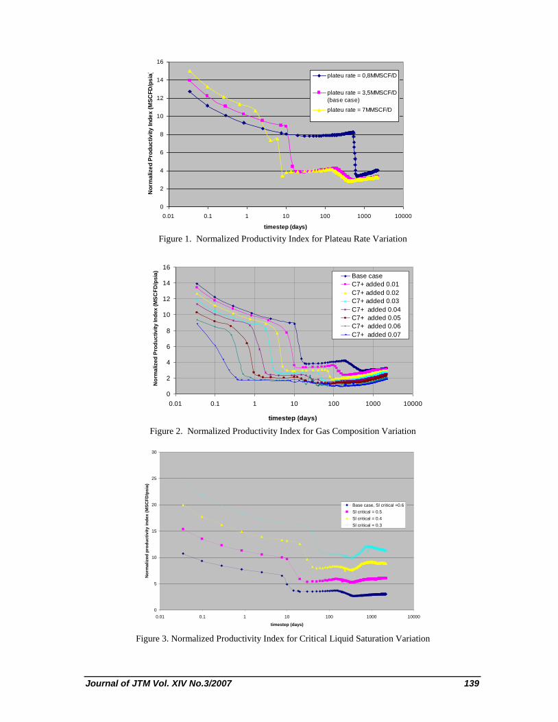
PI calculation is done for each time step in the

simulation. These PI plots for each scenario can

be found in Fig. 1 to Fig. 5. From those plots, it

can be observed that at one certain time point, the

PI will decline suddenly.

Some interesting facts can be derived from these

figures, which are:

At lower gas rate, the productivity will

stay high for a longer time. This can be

seen from Fig. 1.

From Fig. 2, retrograde gas having

heavier component in a higher quantity,

represented by higher C7+ mole fraction,

give poorer productivity and experience

early PI drop.

From Fig. 3, higher critical liquid

saturation also means early PI drop. In

the lowest critical liquid saturation of

0.2, the PI remains relatively high even

though sudden PI drop still occurs.

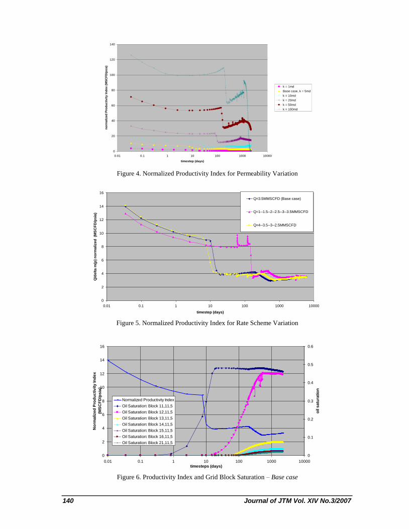
From Fig. 4, higher permeability would

mean greater PI from the beginning.

Although a sudden PI drop occurs for the

high permeability reservoir, the PI value

is still high. A logic conclusion is

because higher permeability would result

in better deliverability since the path

needed for the gas to flow is wider,

although condensation takes place.

The sudden PI drop was observed to be

delayed when the increasing-rate-

gradually scheme was used. In contrary,

if we use the decreasing-rate-gradually

scheme, a sudden PI drop occurs

prematurely.

Further examination can be done using the plot of

condensate saturation changes at certain grid

block. Several grid blocks at the reservoir model

were chosen to represent the whole model,

starting from the block that is perforated (block

11,11,5) until the boundary of the reservoir (block

21,11,5). In these blocks the condensate saturation

changes along with time. The plot for the base

case side by side with PI plot such as in Fig. 6

shows that it is true that sudden PI decline is

caused by the increasing condensate saturation

around the wellbore.

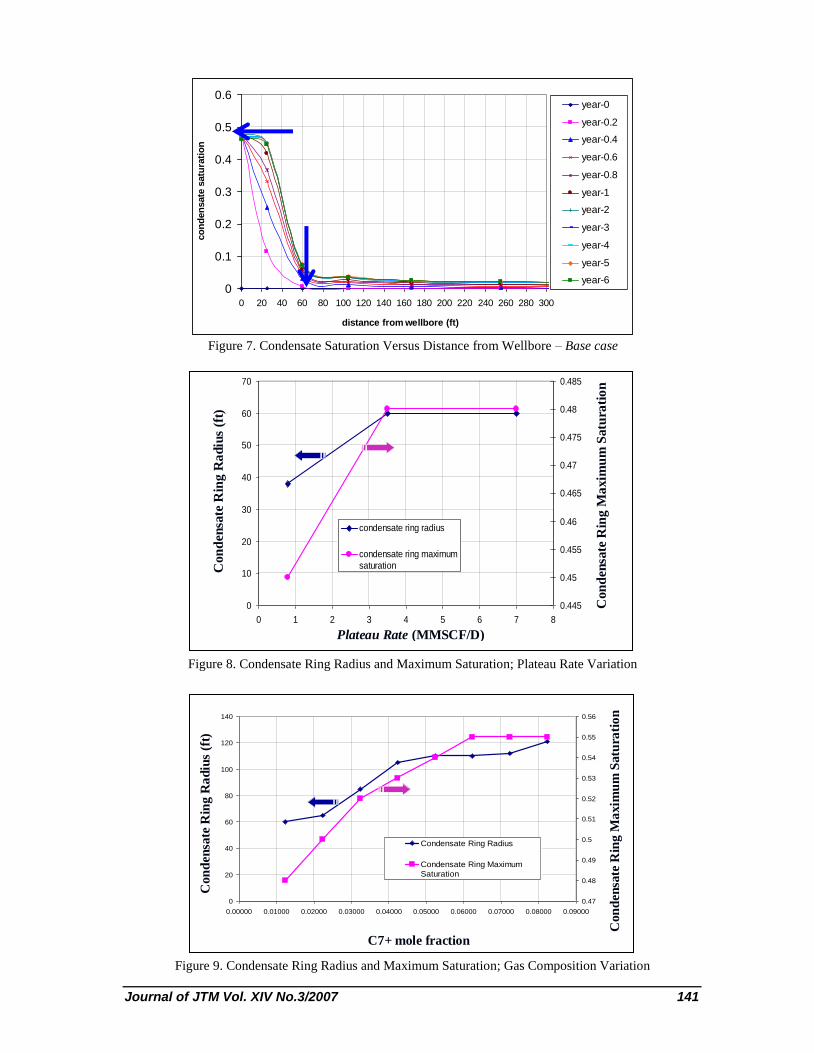
3.2. Condensate Saturation From the simulation, the condensate saturation

can also be plotted versus the distance from the

wellbore, like that in Fig. 7. Such plot is useful in

knowing how much the maximum condensate

saturation circling the wellbore is. And it also can

be used to interpret the radius of the condensate

ring, or how far region 1 extent, in the same

characterization manner used by Fevang and

Whitson.

Figure 7 depicts the saturation–distance plot for

the base case only, changing with time. The other

cases were also checked for the condensate ring

radius and maximum saturation. All of which

display the same typical curves. To make a

connection between how each case responds to

the buildup of condensate saturation, a plot for

every one of the scenarios can be made like in

Figure 8 to Figure 12.

From these figures, several conclusions can be

delivered, such as:

Higher gas rate causes pressure drop to

be higher. If the starting pressure is

already near dew point pressure, then

there will be more condensate liquid

formed. Observing Fig. 8; at higher rate

the condensate ring radius and maximum

saturation both are higher. At rate above

3.5 MMSCF/D the trend seems to be

constant, whereas the truth this is caused

by the limitary of the reservoir model. In

the case of 7 MMSCF/D gas rate, the

reservoir model is too small since it can

not support a long plateau for greater rate

than the base case (3.5 MMSCF/D).

Therefore, the result for 7 MMSCF/D

gas rate case is almost similar like the 3.5

MMSCF/D case.

From Fig. 9, retrograde gas having

heavier component in a greater quantity,

both the condensate ring radius and

maximum saturation will also be higher

since the gas has a higher content of

liquid in it. Also related to gas

composition; it is very advantageous if

the sampling of reservoir fluids are done

as early as possible to prevent

composition change. If the sampling

processes are done after lots of liquid

condense from the gas, then the sample’s

composition would not display the real

behavior at the initial reservoir fluid.

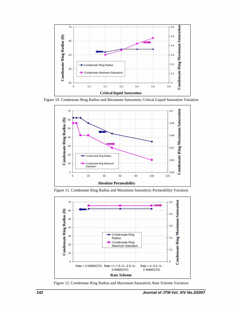
From Fig. 10, higher critical liquid

saturation means the reservoir permits

more condensate saturation to be formed

in the pore space, before able to be

produced. This suggests that condensate

blocking is worsen because there is more

liquid that plug the pore space. In spite of


it, the ring radius seems to be not

influenced.

Higher permeability results in less

condensate ring radius and also less

maximum condensate saturation, as can

be seen from Fig. 11. This is because the

pressure drop is lesser.

From Fig. 12, in every gas rate scheme

tried here, the ring radius and maximum

condensate saturation seemed not to be

affected.

As it was previously thought, condensate blocking

is caused by liquid saturation in pore space,

reducing gas effective permeability and ultimately

causing production decline. So there is a strong

relationship between blocking and condensate

ring radius along with its maximum saturation.

The higher the ring saturation means that blocking

is worsen, while its radius implies how far from

the wellbore this phenomenon occurs.

Also it was observed that in the simulation, the

average condensate saturation is about 0.45, 18

times greater than predicted using the CVD which

is only 0.025. This is due to the fact that CVD

uses a constant volume of gas source in the PVT

cell, while in reality gas continuously flows into

the near well region (as “PVT-cell” analogy) and

condenses liquid along with it. This implies that

one must not ignore the liquid drop from CVD

however small it is.

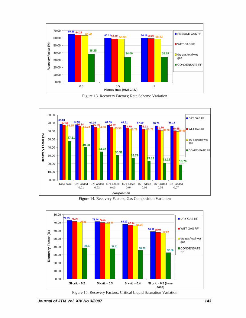
3.3. Recovery Factors The Recovery Factors (RF) were all calculated at

a gas rate of 0.5 MMSCF/D, which is an

assumptions of an economic gas rate.

There are 4 types of RF computed which are

residue gas-RF, wet gas RF, condensate RF, and

the dry gas RF (dry gas produced divided by total

initial wet gas). The first three are based on RF

counting as in a CVD analysis.1 Residue gas RF is

total dry gas produced divided by initial dry gas in

place. Wet gas RF is total wet gas produced

divided by initial wet gas in place. Condensate RF

is total condensate produced divided by initial

condensate in place.

All calculations were plotted in clustered bar

column plot. These plots can be seen in Fig. 13 to

Fig. 17. Conclusions that can be brought are:

From Fig. 13, all the RF are higher for

lower production rate.


low heavy-component gas.


lower critical liquid saturation.

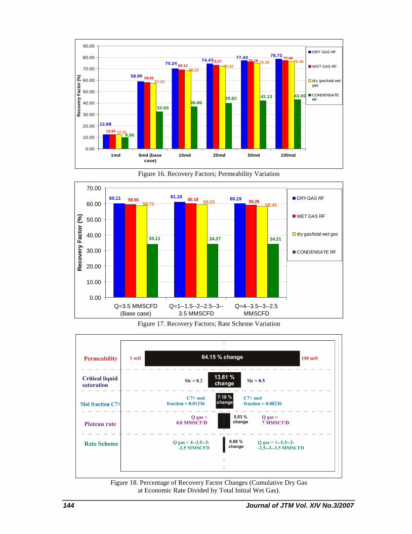
From Figure 16, all the RF are higher for

higher permeability. But the significant

change in RF is for permeability below

10 mD.

From Figure 17, all the RF the highest

RF will be for the increasing-rate-

gradually scheme, although the

difference is not much.

The percentage of RF changes is plotted in Fig.

18. The highest influence of retrograde

condensation is absolute permeability. Meanwhile

critical liquid saturation, C7+ mole fraction,

plateau rate, and rate scheme respectively rank the

2nd

until the 5th

.

In field practice, it is easier to control the gas rate

and the rate scheme. The best way to avoid or to

delay condensate blocking as soon as possible is

by applying low rate and also using the

increasing-rate-gradually scheme. However,

producing low gas rate may not be economical.

More study is needed in the future to relate this

rate choosing from engineering point of view and

economics.

If an operator is dealing with the gas component

problems, such as the gas is very rich, or contains

too much intermediate and heavier components,

the remedial action known to handle it is by

applying lean gas recycling. The lean gas that is a

product from the separator is injected back to the

reservoir, to keep the sub-surface gas composition

the same as long as possible and also giving

pressure support in order to retard the retrograde

condensation. This method will be successful in

gaining more liquid content of the gas, since the

condensate is the most valuable part of the

reservoir fluid, however more investment is

needed to drill more wells for injection, and to

install the facilities needed.

When the field problem is critical liquid saturation

which happened to be too high, another method of

injecting chemicals such as methanol or any other

solvent is worth to be tried. The chemical will

reduce the reservoir’s critical liquid saturation by

somehow affecting its wettability to condensates.

Another method to deal with this problem is by

applying hydraulic fracturing, which will increase

the permeability around the wellbore. Since

condensate blocking does not affect high

permeability reservoirs, more gas will be

recovered from here. This method is also

applicable in repairing tight-permeability

reservoirs.


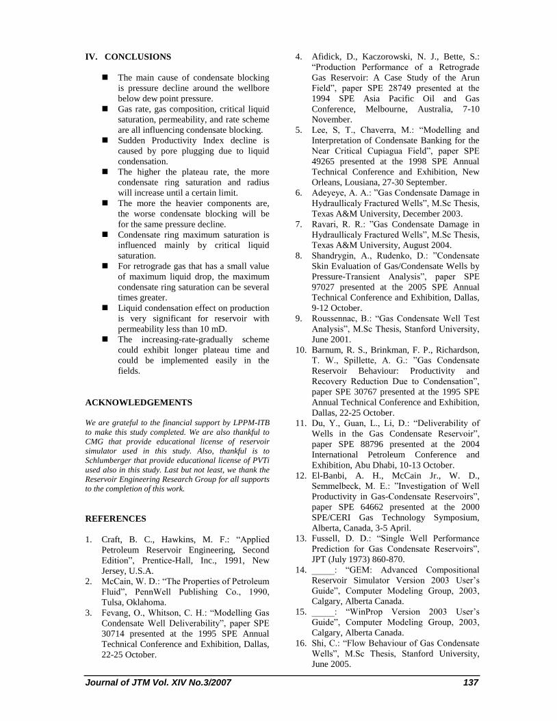
IV. CONCLUSIONS

The main cause of condensate blocking

is pressure decline around the wellbore

below dew point pressure.

Gas rate, gas composition, critical liquid

saturation, permeability, and rate scheme

are all influencing condensate blocking.

Sudden Productivity Index decline is

caused by pore plugging due to liquid

condensation.

The higher the plateau rate, the more

condensate ring saturation and radius

will increase until a certain limit.

The more the heavier components are,

the worse condensate blocking will be

for the same pressure decline.

Condensate ring maximum saturation is

influenced mainly by critical liquid

saturation.

For retrograde gas that has a small value

of maximum liquid drop, the maximum

condensate ring saturation can be several

times greater.

Liquid condensation effect on production

is very significant for reservoir with

permeability less than 10 mD.

The increasing-rate-gradually scheme

could exhibit longer plateau time and

could be implemented easily in the

fields.

ACKNOWLEDGEMENTS

We are grateful to the financial support by LPPM-ITB

to make this study completed. We are also thankful to

CMG that provide educational license of reservoir

simulator used in this study. Also, thankful is to

Schlumberger that provide educational license of PVTi

used also in this study. Last but not least, we thank the

Reservoir Engineering Research Group for all supports

to the completion of this work.

REFERENCES

1. Craft, B. C., Hawkins, M. F.: “Applied

Petroleum Reservoir Engineering, Second

Edition”, Prentice-Hall, Inc., 1991, New

Jersey, U.S.A.

2. McCain, W. D.: “The Properties of Petroleum

Fluid”, PennWell Publishing Co., 1990,

Tulsa, Oklahoma.

3. Fevang, O., Whitson, C. H.: “Modelling Gas

Condensate Well Deliverability”, paper SPE

30714 presented at the 1995 SPE Annual

Technical Conference and Exhibition, Dallas,

22-25 October.

4. Afidick, D., Kaczorowski, N. J., Bette, S.:

“Production Performance of a Retrograde

Gas Reservoir: A Case Study of the Arun

Field”, paper SPE 28749 presented at the

1994 SPE Asia Pacific Oil and Gas

Conference, Melbourne, Australia, 7-10

November.

5. Lee, S, T., Chaverra, M.: “Modelling and

Interpretation of Condensate Banking for the

Near Critical Cupiagua Field”, paper SPE


Technical Conference and Exhibition, New

Orleans, Lousiana, 27-30 September.

6. Adeyeye, A. A.: ”Gas Condensate Damage in

Hydraullicaly Fractured Wells”, M.Sc Thesis,

Texas A&M University, December 2003.

7. Ravari, R. R.: ”Gas Condensate Damage in

Hydraullicaly Fractured Wells”, M.Sc Thesis,

Texas A&M University, August 2004.

8. Shandrygin, A., Rudenko, D.: ”Condensate

Skin Evaluation of Gas/Condensate Wells by

Pressure-Transient Analysis”, paper SPE


Technical Conference and Exhibition, Dallas,

9-12 October.

9. Roussennac, B.: “Gas Condensate Well Test

Analysis”, M.Sc Thesis, Stanford University,

June 2001.

10. Barnum, R. S., Brinkman, F. P., Richardson,

T. W., Spillette, A. G.: ”Gas Condensate

Reservoir Behaviour: Productivity and

Recovery Reduction Due to Condensation”,

paper SPE 30767 presented at the 1995 SPE

Annual Technical Conference and Exhibition,

Dallas, 22-25 October.

11. Du, Y., Guan, L., Li, D.: “Deliverability of

Wells in the Gas Condensate Reservoir”,

paper SPE 88796 presented at the 2004

International Petroleum Conference and

Exhibition, Abu Dhabi, 10-13 October.

12. El-Banbi, A. H., McCain Jr., W. D.,

Semmelbeck, M. E.: ”Investigation of Well

Productivity in Gas-Condensate Reservoirs”,

paper SPE 64662 presented at the 2000

SPE/CERI Gas Technology Symposium,

Alberta, Canada, 3-5 April.

13. Fussell, D. D.: “Single Well Performance

Prediction for Gas Condensate Reservoirs”,

JPT (July 1973) 860-870.

14. _____: “GEM: Advanced Compositional

Reservoir Simulator Version 2003 User’s

Guide”, Computer Modeling Group, 2003,

Calgary, Alberta Canada.

15. _____: “WinProp Version 2003 User’s

Guide”, Computer Modeling Group, 2003,

Calgary, Alberta Canada.

16. Shi, C.: “Flow Behaviour of Gas Condensate

Wells”, M.Sc Thesis, Stanford University,

June 2005.


17. Lee, J., Wattenbarger, R. A.: “Gas Reservoir

Engineering”, Henry L. Doherty Memorial

Fund of AIME, Society of Petroleum

Engineers, 1996, Richardson, Texas.

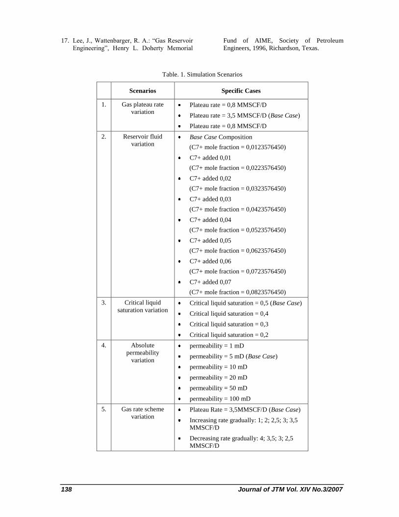
Table. 1. Simulation Scenarios

Scenarios Specific Cases

1. Gas plateau rate

variation Plateau rate = 0,8 MMSCF/D

Plateau rate = 3,5 MMSCF/D (Base Case)

Plateau rate = 0,8 MMSCF/D

2. Reservoir fluid

variation Base Case Composition

(C7+ mole fraction = 0,0123576450)

C7+ added 0,01

(C7+ mole fraction = 0,0223576450)

C7+ added 0,02

(C7+ mole fraction = 0,0323576450)

C7+ added 0,03

(C7+ mole fraction = 0,0423576450)

C7+ added 0,04

(C7+ mole fraction = 0,0523576450)

C7+ added 0,05

(C7+ mole fraction = 0,0623576450)

C7+ added 0,06

(C7+ mole fraction = 0,0723576450)

C7+ added 0,07

(C7+ mole fraction = 0,0823576450)

3. Critical liquid

saturation variation Critical liquid saturation = 0,5 (Base Case)

Critical liquid saturation = 0,4



4. Absolute

permeability

variation

permeability = 1 mD

permeability = 5 mD (Base Case)

permeability = 10 mD




5. Gas rate scheme

variation Plateau Rate = 3,5MMSCF/D (Base Case)

Increasing rate gradually: 1; 2; 2,5; 3; 3,5

MMSCF/D

Decreasing rate gradually: 4; 3,5; 3; 2,5

MMSCF/D


Normalized Productivity Index

0

2

4

6

8

10

12

14

16

0.01 0.1 1 10 100 1000 10000

timestep (days)

No

rma

lize

d P

rod

uc

tiv

ity

In

de

x (

MS

CF

D/p

sia

)

plateu rate = 0,8MMSCF/D

plateu rate = 3,5MMSCF/D

(base case)

plateu rate = 7MMSCF/D

Figure 1. Normalized Productivity Index for Plateau Rate Variation

0

2

4

6

8

10

12

14

16

0.01 0.1 1 10 100 1000 10000

timestep (days)

No

rma

lize

d P

rod

uc

tiv

ity

In

de

x (

MS

CF

D/p

sia

)

Base case

C7+ added 0.01

C7+ added 0.02

C7+ added 0.03

C7+ added 0.04

C7+ added 0.05

C7+ added 0.06

C7+ added 0.07

Figure 2. Normalized Productivity Index for Gas Composition Variation

indeks produktivitas (variasi Saturasi liquid critical)

0

5

10

15

20

25

30

0.01 0.1 1 10 100 1000 10000

timestep (days)

No

rma

lize

d p

rod

uc

tiv

ity

in

de

x (

MS

CF

D/p

sia

)

Base case, Sl critical =0.6

Sl critical = 0.5

Sl critical = 0.4

Sl critical = 0.3

Figure 3. Normalized Productivity Index for Critical Liquid Saturation Variation


Productivity Index (variasi permeabilitas)

0

20

40

60

80

100

120

140

0.01 0.1 1 10 100 1000 10000

timestep (days)

no

rma

lize

d P

rod

uc

tiv

ity

In

de

x (

MS

CF

D/p

sia

)

k = 1md

Base case, k = 5md

k = 10md

k = 20md

k = 50md

k = 100md

Figure 4. Normalized Productivity Index for Permeability Variation

Productivity Index (variasi skema produksi)

0

2

4

6

8

10

12

14

16

0.01 0.1 1 10 100 1000 10000

timestep (days)

Q/d

elt

a m

(p)

no

rma

lize

d (M

SC

FD

/ps

ia)

Q=3.5MMSCFD (Base case)

Q=1--1.5--2--2.5--3--3.5MMSCFD

Q=4--3.5--3--2.5MMSCFD

Figure 5. Normalized Productivity Index for Rate Scheme Variation

0

2

4

6

8

10

12

14

16

0.01 0.1 1 10 100 1000 10000

timesteps (days)

No

rma

lize

d P

rod

uc

tiv

ity

In

de

x

(MS

CF

D/p

sia

)

0

0.1

0.2

0.3

0.4

0.5

0.6

oil s

atu

rati

on

Normalized Productivity Index

Oil Saturation: Block 11,11,5







Figure 6. Productivity Index and Grid Block Saturation – Base case


0

0.1

0.2

0.3

0.4

0.5

0.6

0 20 40 60 80 100 120 140 160 180 200 220 240 260 280 300

distance from wellbore (ft)

co

nd

en

sate

satu

rati

on

year-0

year-0.2

year-0.4

year-0.6

year-0.8

year-1

year-2

year-3

year-4

year-5

year-6

Figure 7. Condensate Saturation Versus Distance from Wellbore – Base case

0

10

20

30

40

50

60

70

0 1 2 3 4 5 6 7 8

0.445

0.45

0.455

0.46

0.465

0.47

0.475

0.48

0.485

condensate ring radius

condensate ring maximum

saturationCon

den

sate

Rin

gR

ad

ius

(ft)

Con

den

sate

Rin

gM

axim

um

Satu

rati

on

Plateau Rate (MMSCF/D)

0

10

20

30

40

50

60

70

0 1 2 3 4 5 6 7 8

0.445

0.45

0.455

0.46

0.465

0.47

0.475

0.48

0.485

condensate ring radius

condensate ring maximum

saturationCon

den

sate

Rin

gR

ad

ius

(ft)

Con

den

sate

Rin

gM

axim

um

Satu

rati

on


Figure 8. Condensate Ring Radius and Maximum Saturation; Plateau Rate Variation

0

20

40

60

80

100

120

140

0.00000 0.01000 0.02000 0.03000 0.04000 0.05000 0.06000 0.07000 0.08000 0.09000

0.47

0.48

0.49

0.5

0.51

0.52

0.53

0.54

0.55

0.56

Condensate Ring Radius

Condensate Ring Maximum

Saturation

Con

den

sate

Rin

g R

ad

ius

(ft)

Con

den

sate

Rin

g M

axim

um

Satu

rati

on

C7+ mole fraction

0

20

40

60

80

100

120

140

0.00000 0.01000 0.02000 0.03000 0.04000 0.05000 0.06000 0.07000 0.08000 0.09000

0.47

0.48

0.49

0.5

0.51

0.52

0.53

0.54

0.55

0.56



Saturation

Con

den

sate

Rin

g R

ad

ius

(ft)

Con

den

sate

Rin

g M

axim

um

Satu

rati

on

C7+ mole fraction

Figure 9. Condensate Ring Radius and Maximum Saturation; Gas Composition Variation


50

55

60

65

70

0 0.1 0.2 0.3 0.4 0.5 0.6

0

0.1

0.2

0.3

0.4

0.5

0.6


Condensate Maximum Saturation

Con

den

sate

Rin

g R

ad

ius

(ft)

Con

den

sate

Rin

gM

axim

um

Satu

rati

on

Critical liquid Saturation

50

55

60

65

70

0 0.1 0.2 0.3 0.4 0.5 0.6

0

0.1

0.2

0.3

0.4

0.5

0.6


Condensate Maximum Saturation

Con

den

sate

Rin

g R

ad

ius

(ft)

Con

den

sate

Rin

gM

axim

um

Satu

rati

on

Critical liquid Saturation

Figure 10. Condensate Ring Radius and Maximum Saturation; Critical Liquid Saturation Variation

0

10

20

30

40

50

60

70

0 20 40 60 80 100 120

0.45

0.46

0.47

0.48

0.49

0.5



Saturation

Con

den

sate

Rin

g R

ad

ius

(ft)

Con

den

sate

Rin

gM

axim

um

Satu

rati

on

Absolute Permeability

0

10

20

30

40

50

60

70

0 20 40 60 80 100 120

0.45

0.46

0.47

0.48

0.49

0.5



Saturation

Con

den

sate

Rin

g R

ad

ius

(ft)

Con

den

sate

Rin

gM

axim

um

Satu

rati

on

Absolute Permeability

Figure 11. Condensate Ring Radius and Maximum Saturation; Permeability Variation

0

10

20

30

40

50

60

70

Rate = 3.5MMSCFD Rate =1--1.5--2—2.5--3--

3.5MMSCFD

Rate = 4--3.5--3--

2.5MMSCFD

0

0.1

0.2

0.3

0.4

0.5

Condensate RingRadius

Condensate RingMaximum Saturation

Con

den

sate

Rin

g R

ad

ius

(ft)

Con

den

sate

Rin

gM

axim

um

Satu

rati

on

Rate Scheme

0

10

20

30

40

50

60

70

Rate = 3.5MMSCFD Rate =1--1.5--2—2.5--3--

3.5MMSCFD

Rate = 4--3.5--3--

2.5MMSCFD

0

0.1

0.2

0.3

0.4

0.5

Condensate RingRadius

Condensate RingMaximum Saturation

Con

den

sate

Rin

g R

ad

ius

(ft)

Con

den

sate

Rin

gM

axim

um

Satu

rati

on

Rate Scheme

Figure 12. Condensate Ring Radius and Maximum Saturation; Rate Scheme Variation


65.29

60.11 60.1659.22 59.27

64.28

58.4358.3863.41

38.2534.00 34.07

0.00

10.00

20.00

30.00

40.00

50.00

60.00

70.00

0.8 3.5 7


Re

co

ve

ry F

ac

tor

(%)

RESIDUE GAS RF

WET GAS RF

dry gas/total wet

gas

CONDENSATE RF

Figure 13. Recovery Factors; Rate Scheme Variation

67.90 67.36 67.59 67.51 67.09 66.74 66.1368.63

66.2467.56

60.4561.7062.7163.7964.5765.03

59.4660.70

66.6565.24 64.03 63.56 62.78 61.71

21.1218.70

26.7730.31

34.72

40.28

47.31

23.62

0.00

10.00

20.00

30.00

40.00

50.00

60.00

70.00

80.00

base case C7+ added

0,01

C7+ added

0,02

C7+ added

0,03

C7+ added

0,04

C7+ added

0,05

C7+ added

0,06

C7+ added

0,07

composition

Re

co

ve

ry F

ac

tor

(%)

DRY GAS RF

WET GAS RF

dry gas/total wetgas

CONDENSATE RF

Figure 14. Recovery Factors; Gas Composition Variation

71.7670.31

58.04

72.9371.44

68.12

58.92

67.1470.83 69.38

66.24

57.22

32.6635.78

37.6138.67

0.00

10.00

20.00

30.00

40.00

50.00

60.00

70.00

80.00

Sl crit. = 0.2 Sl crit. = 0.3 Sl crit. = 0.4 Sl crit. = 0.5 (base

case)

Reco

very

Facto

r (%

)

DRY GAS RF

WET GAS RF

dry gas/total wetgas

CONDENSATERF

Figure 15. Recovery Factors; Critical Liquid Saturation Variation


78.7377.43

74.4770.24

58.90

12.68

77.4676.1873.27

69.13

12.60

58.02

76.4675.2072.32

68.22

57.20

12.31

43.0042.13

32.65

36.8639.82

9.90

0.00

10.00

20.00

30.00

40.00

50.00

60.00

70.00

80.00

90.00

1md 5md (base

case)

10md 20md 50md 100md

Re

co

ve

ry F

ac

tor

(%)

DRY GAS RF

WET GAS RF

dry gas/total wet

gas

CONDENSATE

RF

Figure 16. Recovery Factors; Permeability Variation

60.11 61.10 60.1960.18 59.2959.55

58.4559.3358.71

34.27 34.2134.11

0.00

10.00

20.00

30.00

40.00

50.00

60.00

70.00

Q=3.5 MMSCFD

(Base case)

Q=1--1.5--2--2.5--3--

3.5 MMSCFD

Q=4--3.5--3--2.5

MMSCFD

Reco

very

Facto

r (%

)

DRY GAS RF

WET GAS RF

dry gas/total wet gas

CONDENSATE RF

Figure 17. Recovery Factors; Rate Scheme Variation

Figure 18. Percentage of Recovery Factor Changes (Cumulative Dry Gas

at Economic Rate Divided by Total Initial Wet Gas).

Documents

JTM · PDF fileJournal of JTM Vol. XIV No.3/2007 133 JTM PARAMETRICAL STUDY ON RETROGRADE GAS RESERVOIR BEHAVIOR by: Taufan Marhaendrajana *, Adrian Kartawidjaya